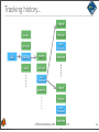
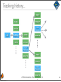
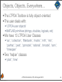
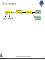
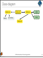
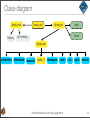
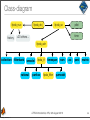
Download LTPDA Introduction, NPL, 9th August 2010

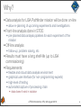
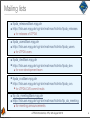
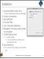
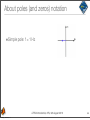
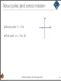
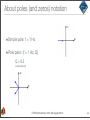
AEI, Hannover
Leibniz Universität Hannover
What is LTPDA?
M Hewitson for the LTP Team
NPL
9th August 2010
Monday, June 20, 11
Outline
• Why LTPDA?
• Formalities
• Installation
• Topic 1: Introducing LTPDA - the basics
• Topic 2: Preprocessing data
• Topic 3: Spectral analysis
• Topic 4: Transfer functions and digital filters
• Topic 5: Fitting data
LTPDA Introduction, NPL, 9th August 2010
Monday, June 20, 11
2
Who he?
• Born in Carlisle
• First 8 years of my working life as electrician
• MSci and PhD from University of Glasgow
• Thesis: “On aspects of characterising and calibrating the
interferometric gravitational wave detector, GEO 600”
• 7 years building, commissioning and calibrating GEO600
• Past 3 years as head of LTP Data Analysis team
• Married, two you children
LTPDA Introduction, NPL, 9th August 2010
Monday, June 20, 11
3
The LTPDA team...
Martin Hewitson
Miquel Nofrarias
Ingo Diepholz
Anneke Monsky
Heather Audley
Mauro Hueller
Luigi Ferraioli
Giuseppe Congedo
Fabrizio De Marchi
Andrea Manica
Andrea Mattioli
Adrien Grynagier
Eric Plagniol
Michele Armano
LTPDA Introduction, NPL, 9th August 2010
Monday, June 20, 11
Marc Diaz Aguiló
4
Not a commercial product!
LTPDA Introduction, NPL, 9th August 2010
Monday, June 20, 11
5
Not a commercial product!
• We have about 2 FTEs currently working on the
toolbox
LTPDA Introduction, NPL, 9th August 2010
Monday, June 20, 11
5
Not a commercial product!
• We have about 2 FTEs currently working on the
toolbox
LTPDA Introduction, NPL, 9th August 2010
Monday, June 20, 11
5
Not a commercial product!
• We have about 2 FTEs currently working on the
toolbox
• Total effort so far is about 10 FTE years
LTPDA Introduction, NPL, 9th August 2010
Monday, June 20, 11
5
Not a commercial product!
• We have about 2 FTEs currently working on the
toolbox
• Total effort so far is about 10 FTE years
LTPDA Introduction, NPL, 9th August 2010
Monday, June 20, 11
5
Not a commercial product!
• We have about 2 FTEs currently working on the
toolbox
• Total effort so far is about 10 FTE years
• Feedback is essential
LTPDA Introduction, NPL, 9th August 2010
Monday, June 20, 11
5
Not a commercial product!
• We have about 2 FTEs currently working on the
toolbox
• Total effort so far is about 10 FTE years
• Feedback is essential
LTPDA Introduction, NPL, 9th August 2010
Monday, June 20, 11
5
Not a commercial product!
• We have about 2 FTEs currently working on the
toolbox
• Total effort so far is about 10 FTE years
• Feedback is essential
• We will help whenever we can
LTPDA Introduction, NPL, 9th August 2010
Monday, June 20, 11
5
Why?
• Data analysis for LISA Pathfinder mission will be done on-line
• allow re-planning of upcoming experiments and investigations
• Front-line analysis done in STOC
• pre-planned data analysis pipelines for each experiment of the
mission
• Off-line analysis
• follow-up, problem solving, etc
• Results must have a long shelf-life (up to LISA
commissioning)
• Requirements:
•
•
•
•
flexible and robust data analysis environment
graphical user interface (for non-programming-experts)
high-level of testing
automated capture of processing chain
• data doesn’t exist in isolation
LTPDA Introduction, NPL, 9th August 2010
Monday, June 20, 11
6
Formalities
• LTPDA:
• http://www.lisa.aei-hannover.de/ltpda/
• Bugs and features:
• https://ed.fbk.eu/ltpda/mantis/
LTPDA Introduction, NPL, 9th August 2010
Monday, June 20, 11
7
Mailing lists
• [email protected]
• http://lists.aei.mpg.de/cgi-bin/mailman/listinfo/ltpda_releases
• for releases of LTPDA
• [email protected]
• http://lists.aei.mpg.de/cgi-bin/mailman/listinfo/ltpda_users
• for LTPDA users
• [email protected]
• http://lists.aei.mpg.de/cgi-bin/mailman/listinfo/ltpda_dev
• for core development team
• [email protected]
• http://lists.aei.mpg.de/cgi-bin/mailman/listinfo/ltpda_cvs
• for LTPDA CVS commit mails
• [email protected]
• http://lists.aei.mpg.de/cgi-bin/mailman/listinfo/ltp_da_meeting
• for meeting announcements
LTPDA Introduction, NPL, 9th August 2010
Monday, June 20, 11
8
Installation
1. Download latest version from
1.1.http://www.lisa.aei-hannover.de/ltpda/
2. Unzip to somewhere
3. Start MATLAB
4. File->Set Path...
5. Click ‘Add with Subfolders...’
6. Navigate to the ltpda_toolbox folder
you unzipped
7. On MATLAB terminal
7.1.>> ltpda_startup
7.1.1.(you can add this command to you
normal startup.m file)
8. Set preferences
8.1.for now just click ‘Apply’ and close the
GUI
LTPDA Introduction, NPL, 9th August 2010
Monday, June 20, 11
9
Post-installation steps
• Test installation
• >> run_tests
• Install graphviz
• see LTPDA user manual (>> doc)
• LTPDA Toolbox
• Getting Started with the LTPDA Toolbox
• Additional 3rd-party software
http://www.lisa.aei-hannover.de/ltpda/usermanual/ug/additional_progs.html
LTPDA Introduction, NPL, 9th August 2010
Monday, June 20, 11
10
Updating the toolbox
• Remove old toolbox from MATLAB path
• File -> Set Path
• Select all in list containing ‘ltpda_toolbox’
• Click ‘Remove’
• Install new toolbox as per previous instructions
LTPDA Introduction, NPL, 9th August 2010
Monday, June 20, 11
11
Submitting a bug or feature request
• Go to https://ed.fbk.eu/ltpda/mantis/
• Self-sign-up
• click ‘Signup for a new account’
• Once your account is active, you can log in
• To report an issue:
• First search the existing issues in case your problem is
covered!
• Click ‘Report Issue’
• Choose project ‘DA_LTPDA’
• Select ‘bug report’ or ‘change request’
• Complete the form with as much information as possible
LTPDA Introduction, NPL, 9th August 2010
Monday, June 20, 11
12
!
Monday, June 20, 11
?
Topic 1
• The basics
•
•
•
•
•
•
•
•
•
•
•
•
•
Object-oriented programming (for beginners)
Analysis Objects
How history tracking works
Other objects
Parameter lists
Building objects
Setting object properties
Viewing history
Making time-series AOs
Basic math
Saving and loading
Reading data files
Writing LTPDA scripts
• Hands-on
+----------------------------------------------------+
|
|
|
|
|
****
|
|
**
|
|
------------|
|
////
/
\\\\
|
|
///
/
\\\
|
|
|
/
|
|
|
** |
+----+ /
+----+
| **
|
|
***|
|
|//-------|
|
|***
|
|
** |
+----+
/+----+
| **
|
|
|
/
|
|
|
\\\
/
///
|
|
\\\\
//
////
|
|
------------|
|
**
|
|
****
|
|
|
|
Welcome to LTPDA Toolbox
|
|
|
|
Version: 2.3.1
|
|
Release: (R2010a)
|
|
Date: 30-07-10
|
|
|
+----------------------------------------------------+
LTPDA Introduction, NPL, 9th August 2010
Monday, June 20, 11
14
Object-oriented programming
• Learn these words:
• class
• object
• instance
• method
• constructor
• property
• inheritance
LTPDA Introduction, NPL, 9th August 2010
Monday, June 20, 11
15
Class
• A class is a description of an object
• Examples:
• aeroplane, house, vehicle, animal
• algorithm, colour, sentence
LTPDA Introduction, NPL, 9th August 2010
Monday, June 20, 11
16
Class
• A class is a description of an object
• Examples:
• aeroplane, house, vehicle, animal
• algorithm, colour, sentence
LTPDA Introduction, NPL, 9th August 2010
Monday, June 20, 11
16
Object, instance
• An object is an instance of a class
• Examples:
• Airforce 1 (aeroplane), me (person), garfield (cartoon
cat)
• mean (algorithm), red (color), “isn’t this
easy?” (sentence)
LTPDA Introduction, NPL, 9th August 2010
Monday, June 20, 11
17
Object, instance
• An object is an instance of a class
• Examples:
• Airforce 1 (aeroplane), me (person), garfield (cartoon
cat)
• mean (algorithm), red (color), “isn’t this
easy?” (sentence)
LTPDA Introduction, NPL, 9th August 2010
Monday, June 20, 11
17
method
• Something that acts on an object (instance of a
class)
• Examples:
• ‘start’ a ‘car’ - ‘start’ is a method of the class ‘car’
• ‘start’ my car - use the method ‘fly’ on my car
• mean(x) - use the method ‘mean’ on the data object ‘x’
LTPDA Introduction, NPL, 9th August 2010
Monday, June 20, 11
18
method
• Something that acts on an object (instance of a
class)
• Examples:
• ‘start’ a ‘car’ - ‘start’ is a method of the class ‘car’
• ‘start’ my car - use the method ‘fly’ on my car
• mean(x) - use the method ‘mean’ on the data object ‘x’
LTPDA Introduction, NPL, 9th August 2010
Monday, June 20, 11
18
construct
• A special method of a class which builds an
instance of the class (builds an object)
• normally the method has the same name as the class
• Examples:
• car(‘blue’) - builds a blue car
• animal(‘dog’, ‘brown’) - builds a brown dog which is a
type of animal
LTPDA Introduction, NPL, 9th August 2010
Monday, June 20, 11
19
construct
• A special method of a class which builds an
instance of the class (builds an object)
• normally the method has the same name as the class
• Examples:
• car(‘blue’) - builds a blue car
• animal(‘dog’, ‘brown’) - builds a brown dog which is a
type of animal
LTPDA Introduction, NPL, 9th August 2010
Monday, June 20, 11
19
property
• A property is one aspect of a class (or object)
• Examples:
• a ‘car’ might have properties:
• make, color, top-speed, cost
• an algorithm might have properties
• input-type, different configuration parameters
LTPDA Introduction, NPL, 9th August 2010
Monday, June 20, 11
20
property
• A property is one aspect of a class (or object)
• Examples:
• a ‘car’ might have properties:
• make, color, top-speed, cost
• an algorithm might have properties
• input-type, different configuration parameters
LTPDA Introduction, NPL, 9th August 2010
Monday, June 20, 11
20
inheritance
• classes can inherit behaviour (methods and
properties) from other classes
vehicle
-color
+start
boat
wheeled
-# sails
-# wheels
bicycle
+ start
car
- engine size
+ start
LTPDA Introduction, NPL, 9th August 2010
Monday, June 20, 11
21
inheritance
• classes can inherit behaviour (methods and
properties) from other classes
vehicle
-color
+start
boat
wheeled
-# sails
-# wheels
bicycle
+ start
car
- engine size
+ start
LTPDA Introduction, NPL, 9th August 2010
Monday, June 20, 11
21
!
Monday, June 20, 11
?
Analysis Objects
• Aim to store data products
Analysis Object
- Name
- Numerical data
vectors
- Creation date/time
- Additional flags
-
Name
ID number
Comment
pipeline file(s)
Numerical
Data
Provenance
Additional
meta-data
Processing
history
-
creator
date
IP address
Hostname
Operating System
software versions
-
Name
Algorithm version
Parameter list
Creation date/time
Input histories
LTPDA Introduction, NPL, 9th August 2010
Monday, June 20, 11
23
AO Methods
>> methods ao
Contents
abs
acos
angle
ao
asin
atan
atan2
bilinfit
bin_data
bsubmit
buildWhitener1D
cat
char
cohere
complex
compute
confint
conj
consolidate
conv
convert
copy
corr
cos
cov
cpsd
crbound
created
creator
csvexport
ctranspose
curvefit
delay
delayEstimate
demux
det
Monday, June 20, 11
detrend
dft
diag
diff
display
dopplercorr
downsample
dropduplicates
dsmean
dx
dy
eig
eq
eqmotion
evaluateModel
exp
export
fft
fftfilt
filtSubtract
filter
filtfilt
find
firwhiten
fixfs
fngen
fromProcinfo
fs
gapfilling
gapfillingoptim
ge
get
getdof
gnuplot
gt
heterodyne
hist
hist_gauss
hypot
ifft
imag
index
integrate
interp
interpmissing
inv
iplot
iplotyy
isprop
isvalid
join
lcohere
lcpsd
le
len
linSubtract
lincom
linedetect
linfit
lisovfit
ln
log
log10
lpsd
lscov
lt
ltfe
ltp_ifo2acc
max
mcmc
md5
mdc1_cont2act_utn
mdc1_ifo2acc_fd
mdc1_ifo2acc_fd_utn
mdc1_ifo2acc_inloop
mdc1_ifo2cont_utn
mdc1_ifo2control
mdc1_x2acc
mean
median
min
minus
mode
mpower
mrdivide
mtimes
ne
noisegen1D
noisegen2D
norm
normdist
nsecs
offset
optSubtraction
phase
plot
plus
polyfit
polynomfit
power
psd
psdconf
pwelch
quasiSweptSine
rdivide
real
rebuild
removeVal
report
resample
rms
rotate
round
sDomainFit
save
scale
scatterData
search
select
setDescription
setDx
setDy
setFs
setMdlfile
setName
setPlotinfo
setProcinfo
setT0
setUUID
setX
setXY
setXunits
setY
setYunits
setZ
sign
simplifyYunits
sin
sineParams
smallvector_lincom
smallvectorfit
smoother
sort
spectrogram
spikecleaning
split
spsd
sqrt
LTPDA Introduction, NPL, 9th August 2010
std
straightLineFit
string
submit
sum
sumjoin
svd
svd_fit
t0
table
tan
tdfit
tfe
timeaverage
timedomainfit
times
timeshift
transpose
type
uminus
unwrap
update
upsample
validate
var
viewHistory
whiten1D
whiten2D
x
xcorr
xfit
xunits
y
yunits
zDomainFit
zeropad
24
Tracking history...
ao
LTPDA Introduction, NPL, 9th August 2010
Monday, June 20, 11
25
Tracking history...
name
version
ao
history
data
LTPDA Introduction, NPL, 9th August 2010
Monday, June 20, 11
25
Tracking history...
name
version
ao
history
name
data
version
input
histories
params
LTPDA Introduction, NPL, 9th August 2010
Monday, June 20, 11
25
Tracking history...
name
ao
name
version
version
input
histories
history
name
data
version
params
input
histories
params
LTPDA Introduction, NPL, 9th August 2010
Monday, June 20, 11
25
Tracking history...
name
ao
name
version
version
input
histories
history
name
data
version
params
input
histories
params
name
version
input
histories
params
LTPDA Introduction, NPL, 9th August 2010
Monday, June 20, 11
25
Tracking history...
name
ao
name
version
version
input
histories
history
name
data
version
params
input
histories
params
name
version
input
histories
params
LTPDA Introduction, NPL, 9th August 2010
Monday, June 20, 11
25
Smart algorithms
Intelligent algorithms
Algorithmic step
Input
AO
input
history
Algorithm
history
Input
AO
Output
AO(s)
input
history
traceable results
LTPDA Introduction, NPL, 9th August 2010
Monday, June 20, 11
26
Viewing history
LTPDA Introduction, NPL, 9th August 2010
Monday, June 20, 11
27
Reliving history
obj.type(<file>)
output commands needed
to rebuild this object
robj = obj.rebuild
rebuild this object
LTPDA Introduction, NPL, 9th August 2010
Monday, June 20, 11
28
Objects, Objects, Everywhere...
• The LTPDA Toolbox is fully object-oriented
• The user deals with:
• ‘LTPDA user objects’
• MATLAB primitives (strings, doubles, logicals, etc)
• We have 13 LTPDA User Classes
• 'ao', 'collection', 'filterbank', 'matrix', 'mfir', 'miir',
'parfrac', 'pest', 'pzmodel', 'rational', 'smodel', 'ssm',
'timespan'
• Two ‘helper’ classes
• ‘plist’, ‘time’
LTPDA Introduction, NPL, 9th August 2010
Monday, June 20, 11
29
Class-diagram
ltpda_obj
LTPDA Introduction, NPL, 9th August 2010
Monday, June 20, 11
30
Class-diagram
ltpda_nuo
ltpda_obj
LTPDA Introduction, NPL, 9th August 2010
Monday, June 20, 11
30
Class-diagram
ltpda_nuo
ltpda_obj
ltpda_uo
LTPDA Introduction, NPL, 9th August 2010
Monday, June 20, 11
30
Class-diagram
ltpda_nuo
ltpda_obj
ltpda_uo
plist
time
LTPDA Introduction, NPL, 9th August 2010
Monday, June 20, 11
30
Class-diagram
ltpda_nuo
history
ltpda_obj
ltpda_uo
time
+20 others...
LTPDA Introduction, NPL, 9th August 2010
Monday, June 20, 11
plist
30
Class-diagram
ltpda_nuo
history
ltpda_obj
ltpda_uo
plist
time
+20 others...
ltpda_uoh
LTPDA Introduction, NPL, 9th August 2010
Monday, June 20, 11
30
Class-diagram
ltpda_obj
ltpda_nuo
history
plist
ltpda_uo
time
+20 others...
ltpda_uoh
collection
filterbank
smodel
ltpda_tf
timespan
ssm
LTPDA Introduction, NPL, 9th August 2010
Monday, June 20, 11
ao
pest
matrix
30
Class-diagram
ltpda_obj
ltpda_nuo
history
plist
ltpda_uo
time
+20 others...
ltpda_uoh
collection
filterbank
smodel
rational
ltpda_tf
parfrac
timespan
ltpda_filter
ssm
pest
matrix
pzmodel
LTPDA Introduction, NPL, 9th August 2010
Monday, June 20, 11
ao
30
Class-diagram
ltpda_obj
ltpda_nuo
history
plist
ltpda_uo
time
+20 others...
ltpda_uoh
collection
filterbank
smodel
rational
ltpda_tf
parfrac
timespan
ltpda_filter
miir
ssm
pest
matrix
pzmodel
mfir
LTPDA Introduction, NPL, 9th August 2010
Monday, June 20, 11
ao
30
Parameter lists
• Essentially all methods and constructors are
configured by parameter lists (plists)
• A parameter list has:
• a list of parameters
• a name (inherited)
• a description (inherited)
• a UUID* (inherited)
• Each parameter has a ‘key’ and a ‘value’
• key == string
• value == MATLAB primitive or LTPDA object
*http://en.wikipedia.org/wiki/UUID
LTPDA Introduction, NPL, 9th August 2010
Monday, June 20, 11
31
Examples:
>> pl = plist
----------- plist 01 ----------n params: 0
description:
UUID:
9d9ef3a6-52f1-4fbf-a442-f83d9d7b6b88
--------------------------------
Empty Parameter List
>> pl = plist('a', 1, 'b', 'two')
----------- plist 01 ----------n params: 2
---- param 1 ---key: A
val: 1
-------------------- param 2 ---key: B
val: 'two'
----------------description:
UUID:
d4b59063-292c-4254-b562-0fef3fb11c17
--------------------------------
Parameter list with
two parameters, ‘a’
and ‘b’
LTPDA Introduction, NPL, 9th August 2010
Monday, June 20, 11
32
Building objects
• Objects are built using class constructors:
• object = <class_name>(<arguments>)
• Examples:
>> a = ao
>> a = ao(1)
>> a = ao(plist(‘vals’, 1))
>> s = smodel(‘a*x+b’)
>> s = mfir(‘filter.xml’)
>> pl = plist(‘filename’, ‘filter.xml’)
>> s = mfir(pl)
empty analysis object
analysis object with a single data value
as above, using a plist
symbolic model of a straight-line
build an FIR filter by loading it from a file
as above, using a plist
LTPDA Introduction, NPL, 9th August 2010
Monday, June 20, 11
33
Getting help
• How do I know which parameters to put in my
plist?
>> help mfir
MFIR FIR filter object class constructor.
%%%%%%%%%%%%%%%%%%%%%%%%%%%%%%%%%%%%%%%%%%%%%%%%%%%%%%%%%%%%%%%%%%%%%%%%%%%%%%
DESCRIPTION: MFIR FIR filter object class constructor.
Create a mfir object.
CONSTRUCTORS:
f = mfir()
- creates an empty mfir object.
:
:
Parameter Sets
VERSION:
$Id: mfir.m,v 1.103 2010/05/05 09:30:07 ingo Exp $
SEE ALSO:
miir, ltpda_filter, ltpda_uoh, ltpda_uo, ltpda_obj, plist
%%%%%%%%%%%%%%%%%%%%%%%%%%%%%%%%%%%%%%%%%%%%%%%%%%%%%%%%%%%%%%%%%%%%%%%%%%%%%%
LTPDA Introduction, NPL, 9th August 2010
Monday, June 20, 11
34
Getting help
• How do I know which parameters to put in my
plist?
>> help mfir
MFIR FIR filter object class constructor.
%%%%%%%%%%%%%%%%%%%%%%%%%%%%%%%%%%%%%%%%%%%%%%%%%%%%%%%%%%%%%%%%%%%%%%%%%%%%%%
DESCRIPTION: MFIR FIR filter object class constructor.
Create a mfir object.
CONSTRUCTORS:
f = mfir()
- creates an empty mfir object.
:
:
Parameter Sets
click here
VERSION:
$Id: mfir.m,v 1.103 2010/05/05 09:30:07 ingo Exp $
SEE ALSO:
miir, ltpda_filter, ltpda_uoh, ltpda_uo, ltpda_obj, plist
%%%%%%%%%%%%%%%%%%%%%%%%%%%%%%%%%%%%%%%%%%%%%%%%%%%%%%%%%%%%%%%%%%%%%%%%%%%%%%
LTPDA Introduction, NPL, 9th August 2010
Monday, June 20, 11
34
LTPDA Introduction, NPL, 9th August 2010
Monday, June 20, 11
35
Getting more help
• LTPDA Toolbox has a decent amount of
documentation:
• >> doc ltpda
• Which methods are available?
• >> methods <class_name>
• example:
>> methods mfir
Methods for class mfir:
Contents
bsubmit
char
copy
created
creator
csvexport
display
eq
get
impresp
index
isprop
isvalid
mfir
ne
rebuild
redesign
report
resp
save
setA
setDescription
setHistout
setIunits
setMdlfile
setName
setOunits
LTPDA Introduction, NPL, 9th August 2010
Monday, June 20, 11
setPlotinfo
setProcinfo
setUUID
simplifyUnits
string
submit
type
update
viewHistory
36
Setting object properties
• Properties of an object can be set using ‘setter’
methods, or during construction:
>> a = ao(plist('name', 'bob'))
----------- ao 01: bob ----------name: bob
data: None
hist: ao / ao / $Id: ao.m,v 1.315 2010/06/25 13:55:38 ingo Exp $
mdlfile: empty
description:
UUID: 500458d6-2a4d-42a9-8d25-3fe5ebd1548f
--------------------------------->> a = ao;
>> a.setName('bob')
----------- ao 01: bob ----------name: bob
data: None
hist: ltpda_uoh / setName / $Id: setName.m,v 1.12 2010/06/07 16:35:26
ingo Exp $
mdlfile: empty
description:
UUID: 7172543d-e69d-4fcf-abdd-b111b9c16434
LTPDA Introduction, NPL, 9th August 2010
---------------------------------Monday, June 20, 11
37
Modifying or copying...
• Many methods can be used to modify existing
objects; some methods create new objects
• Modifying:
• >> a.setName(‘bob’)
• the object ‘a’ will be modified and its name changed
• Copying:
• >> b = a.setName(‘bob’)
• object ‘a’ will be copied. The copy will get the name ‘bob’
and ‘a’ will be left intact
• Some methods can not be used as modifiers
LTPDA Introduction, NPL, 9th August 2010
Monday, June 20, 11
38
Help!
• Which properties does an object have?
• >> properties <class_name>
• >> properties(object)
Note: some properties are read-only. You need to check
for the existence of a setter method like ‘setName’.
These methods take care of the history for you!
LTPDA Introduction, NPL, 9th August 2010
Monday, June 20, 11
39
Viewing history
• We have two static ‘viewers’:
• using graphviz (recall the introduction)
• outputs vector graphics so can be used for huge history
trees
• using matlab
• suitable for small history trees only
• Use graphical explorer
• >> ltpda_explorer(obj)
• Look at the commands:
• >> type(obj)
LTPDA Introduction, NPL, 9th August 2010
Monday, June 20, 11
40
Viewing history
• We have two static ‘viewers’:
• using graphviz (recall the introduction)
• outputs vector graphics so can be used for huge history
trees
• using matlab
• suitable for small history trees only
>> type(a)
-------------------------------------------------------------------------bob-------------------------------------------------------------------------
• Use graphical explorer
• >> ltpda_explorer(obj)
a2812886 = ao([plist()]); % ao
a2818295 = setName(a2812886, [plist('NAME', 'bob')]); % ltpda_uoh
a_out = a2818295;
• Look at the commands:
• >>-------------------------------------------------type(obj)
------------------------bob-------------------------------------------------------------------------
LTPDA Introduction, NPL, 9th August 2010
Monday, June 20, 11
40
Build a time-series AO
• AOs can contain different types of data
• Time-series data are stored in a tsdata object
• In this case, the ao.data field will be a tsdata object
• They also have properties:
tsdata
t0
Absolute time-stamp
of first sample
xunits
X-axis units
yunits
Y-axis units
• Constructors:
• a = ao(vector, sample_rate)
• a = ao(plist('tsfcn', 't.^2 + t', 'fs', 10, 'nsecs', 1000))
• others: >> help ao, click ‘Parameter Sets’
LTPDA Introduction, NPL, 9th August 2010
Monday, June 20, 11
41
Basic Math
• You can operate on AOs using a large set of
methods
• In particular, many typical Math operations are available
(overloaded)
• Further details at: http://www.lisa.aei-hannover.de/ltpda/
documents/files/operator_rules.pdf
a = ao(1);
b = ao(2);
c = a+b
a = ao(2);
a.^2
a = [ao(1) ao(2) ao(3)];
b = ao(4);
c = a + b
LTPDA Introduction, NPL, 9th August 2010
Monday, June 20, 11
42
Saving and loading objects
• All LTPDA User Objects can be saved to (and
loaded from), file in
• XML format
• binary MAT format
<?xml version="1.0" encoding="utf-8"?>
>>
>>
>>
>>
>>
>>
save(a, 'foo.xml')
save(a, 'foo.mat')
a.save(plist('filename',
b = ao('foo.xml')
c = ao('foo.mat')
d = ao(plist('filename',
Monday, June 20, 11
<ltpda_object ltpda_version="2.0 (R2008b)">
<object shape="1x1" type="ao">
<property prop_name="data" shape="1x1" type="fsdata">
<object shape="1x1" type="fsdata">
<property prop_name="t0" shape="1x1" type="time">
<object shape="1x1" type="time">
<property prop_name="utc_epoch_milli" shape="1x1"
<property prop_name="timezone" shape="1x1" type="s
'foo.xml'))
<property prop_name="timeformat" shape="1x23" type
<property prop_name="time_str" shape="0x0" type="c
<property prop_name="version" shape="1x53" type="c
</object>
'foo.xml'))
</property>
<property prop_name="navs" shape="1x1" type="double">1</
<property prop_name="fs" shape="1x1" type="double">1000<
<property prop_name="enbw" shape="1x1" type="double">0.2
<property prop_name="version" shape="1x55" type="char">$
<property prop_name="xunits" shape="1x1" type="unit">
<object shape="1x1" type="unit">
<property prop_name="strs" shape="1x1" type="cell"
43
LTPDA Introduction, NPL, 9th August 2010
Reading existing data files
• You can construct AOs from existing ASCII (raw)
data files
a = ao('topic1/simpleASCII.txt')
sigs = ao(plist('filename', 'topic1/multicolumnASCII.txt', ...
'columns', [1 3 1 5], ...
'name', {'sin2', 'sin4'}, ...
'yunits', {'m', 'm'}, ...
'description', {'sine wave at 2Hz', 'sine wave at 4Hz'}))
LTPDA Introduction, NPL, 9th August 2010
Monday, June 20, 11
44
Hands on the keys...
• You can work through these concepts in the
relevant section of the documentation
• “LTPDA Training Session 1”
LTPDA Introduction, NPL, 9th August 2010
Monday, June 20, 11
45
!
Monday, June 20, 11
?
Introducing the workbench
LTPDA Introduction, NPL, 9th August 2010
Monday, June 20, 11
47
Introducing the workbench
Graphical editor for LTPDA commands
LTPDA Introduction, NPL, 9th August 2010
Monday, June 20, 11
47
Introducing the workbench
Graphical editor for LTPDA commands
Create multiple pipelines in one workbench
LTPDA Introduction, NPL, 9th August 2010
Monday, June 20, 11
47
Introducing the workbench
Graphical editor for LTPDA commands
Create multiple pipelines in one workbench
Edit block parameter lists in place
LTPDA Introduction, NPL, 9th August 2010
Monday, June 20, 11
47
Introducing the workbench
Graphical editor for LTPDA commands
Create multiple pipelines in one workbench
Edit block parameter lists in place
Create (reusable) subsystems
LTPDA Introduction, NPL, 9th August 2010
Monday, June 20, 11
47
Introducing the workbench
Graphical editor for LTPDA commands
Create multiple pipelines in one workbench
Drag-n-drop access to all LTPDA methods
Edit block parameter lists in place
Create (reusable) subsystems
LTPDA Introduction, NPL, 9th August 2010
Monday, June 20, 11
47
Parameter list editing
LTPDA Introduction, NPL, 9th August 2010
Monday, June 20, 11
48
Parameter list editing
Different parameter sets
LTPDA Introduction, NPL, 9th August 2010
Monday, June 20, 11
48
Parameter list editing
Different parameter sets
Parameter ‘key’
LTPDA Introduction, NPL, 9th August 2010
Monday, June 20, 11
48
Parameter list editing
Different parameter sets
Parameter ‘key’
Parameter ‘value’
LTPDA Introduction, NPL, 9th August 2010
Monday, June 20, 11
48
Parameter list editing
Different parameter sets
Parameter ‘key’
Parameter ‘value’
Open ‘special’ editor
LTPDA Introduction, NPL, 9th August 2010
Monday, June 20, 11
48
Parameter list editing
Different parameter sets
Parameter ‘key’
Parameter ‘value’
Open ‘special’ editor
Activate/de-activate a
parameter
LTPDA Introduction, NPL, 9th August 2010
Monday, June 20, 11
48
Parameter list editing
Different parameter sets
Parameter ‘key’
Parameter ‘value’
Open ‘special’ editor
Activate/de-activate a
parameter
Add/remove a parameter
LTPDA Introduction, NPL, 9th August 2010
Monday, June 20, 11
48
Parameter list editing
Different parameter sets
Parameter ‘key’
Parameter ‘value’
Open ‘special’ editor
Activate/de-activate a
parameter
Add/remove a parameter
‘Set’ a parameter set
LTPDA Introduction, NPL, 9th August 2010
Monday, June 20, 11
48
Special blocks
LTPDA Introduction, NPL, 9th August 2010
Monday, June 20, 11
49
Special blocks
Annotation
LTPDA Introduction, NPL, 9th August 2010
Monday, June 20, 11
49
Special blocks
Annotation
MATLAB
Expressions
LTPDA Introduction, NPL, 9th August 2010
Monday, June 20, 11
49
Special blocks
Annotation
MATLAB
Expressions
MATLAB
Function
LTPDA Introduction, NPL, 9th August 2010
Monday, June 20, 11
49
Special blocks
Annotation
MATLAB
Expressions
MATLAB
Function
Constant
LTPDA Introduction, NPL, 9th August 2010
Monday, June 20, 11
49
Special blocks
Annotation
MATLAB
Expressions
MATLAB
Function
Mux/Demux
Constant
LTPDA Introduction, NPL, 9th August 2010
Monday, June 20, 11
49
Special blocks
Annotation
Export objects
to workspace
MATLAB
Expressions
MATLAB
Function
Mux/Demux
Constant
LTPDA Introduction, NPL, 9th August 2010
Monday, June 20, 11
49
Special blocks
Import objects
from another
pipeline
Annotation
Export objects
to workspace
MATLAB
Expressions
MATLAB
Function
Mux/Demux
Constant
LTPDA Introduction, NPL, 9th August 2010
Monday, June 20, 11
49
Shortcut keys
ctrl-s
Save workbench
ctrl-n
New pipeline in current workbench
ctrl-c,ctrl-v,ctrl-d
copy, paste, duplicate
ctrl-t
comment-out block(s)
ctrl-b
quick-block dialog
ctrl-i
edit canvas info
ctrl-f
find blocks in workbench
shift-F1
help on selected block
LTPDA Introduction, NPL, 9th August 2010
Monday, June 20, 11
50
Workbench Fix
• copy reset.m to
<somewhere>/ltpda_toolbox_2.3/ltpda/classes/
@LTPDAworkbench/reset.m
LTPDA Introduction, NPL, 9th August 2010
Monday, June 20, 11
51
!
Monday, June 20, 11
?
Interferometer-Temperature example
• We have a data analysis exercise which will
develop fully over the course of the training
session
• This is the first part: reading and preparing the data
• Work through help section
• Topic 1
• IFO/Temperature Example - Introduction
LTPDA Introduction, NPL, 9th August 2010
Monday, June 20, 11
53
!
Monday, June 20, 11
?
Topic 2: Pre-processing data
• Why?
• data preparation for further analysis
• LTPDA contains a bunch of functions for
• resampling data
• interpolation of data
• de-trending data
• noise whitening
• data selection
LTPDA Introduction, NPL, 9th August 2010
Monday, June 20, 11
55
Look in the help!
LTPDA Introduction, NPL, 9th August 2010
Monday, June 20, 11
56
Resampling
• Integer factor
• Down-sample (ao/downsample)
• for example, to reduce data load
• Up-sample (ao/upsample)
• for example, to match sample rates, do ‘better’ filtering
• Re-sample (ao/resample)
• fs_out = P/Q * fs_in (P and Q are integers)
LTPDA Introduction, NPL, 9th August 2010
Monday, June 20, 11
57
Topic 2 - Exercises 1,2,3
• Open MATLAB documentation
• In the MATLAB terminal
• >> doc
• “Help -> Product Help>”
• work through
• LTPDA Toolbox - LTPDA Training Session 1 Topic 2
• Downsampling
• Upsampling
• Resampling
LTPDA Introduction, NPL, 9th August 2010
Monday, June 20, 11
58
Interpolation
work through:
Topic 2- Interpolation
LTPDA Introduction, NPL, 9th August 2010
Monday, June 20, 11
59
Interpolation
‘vertices’
new time grid
interpolation methods
‘linear’
linear interpolation
‘spline’
spline interpolation
‘cubic’
cubic interpolation
‘nearest’
nearest neighbour
work through:
Topic 2- Interpolation
LTPDA Introduction, NPL, 9th August 2010
Monday, June 20, 11
59
Detrending data
• Remove trends by
• subtracting polynomial fit from data
• ao/detrend calls MATLABs polyfit
work through:
Topic 2- Removing trends
LTPDA Introduction, NPL, 9th August 2010
Monday, June 20, 11
60
Whitening
• The LTDA Toolbox offers various ways to whiten
your data
• with a known filter
• build filter and apply it to your data
• with a known model of spectral content
• use whiten1D
• for single, uncorrelated data streams
• whiten2D
• for a pair of correlated data streams
• without model (Exercise)
• let whiten1D fit a model to the spectrum of your data
work through
Topic 2 whitening
LTPDA Introduction, NPL, 9th August 2010
Monday, June 20, 11
61
Select & find/ split & join
• Chose the samples you want to analyse
• find/select data samples by its properties
• sample numbers - ‘select’
• query for x and y values - ‘find’
• split data by
• intervals, times, frequencies, samples
• Group of functions helps you to
• for find and select exactly the data you want split your
data into pieces and eventually
• join them back together
work through
Topic 2 - select and find, split and join
LTPDA Introduction, NPL, 9th August 2010
Monday, June 20, 11
62
Pre-processing the IFO/Temp data
• There is a useful function which ‘cleans up’ the
data
• consolidate
• consolidate fixes our two data streams such
that
• they start at the same time
• they have the same sampling rate
• the are evenly sample on the same grid
• Work through
• LTPDA Toolbox - LTPDA Training Session 1, Topic 2
• IFO/Temp example
LTPDA Introduction, NPL, 9th August 2010
Monday, June 20, 11
63
!
Monday, June 20, 11
?
Power Spectral Density Estimation (1)
Definition:
1
Pxx ( f ) =
fs
+∞
∑ R ( m ) exp(−2π i ⋅ f ⋅ m
xx
fs )
m = −∞
Estimates the one-sided PSD:
⎧
fs
- ≤ f ≤0
⎪ 0,
⎪
2

Pxx ( f ) = ⎨
⎪ 2P ( f ) , 0 ≤ f ≤ fs
xx
⎪⎩
2
LTPDA Introduction, NPL, 9th August 2010
Monday, June 20, 11
⎫
⎪
⎪
⎬
⎪
⎪⎭
65
Power Spectral Density Estimation (2)
• The PSD at each frequency is estimated via the
Welch method:
• Given a discretized signal x[n] of length N, Data are
divided into segments of length L and multiplied by a
window
• this also reduces the edge-effects (simulating a periodic
sequence)
• The PSD at each frequency f is estimated as:
2
XL
P̂xx ( f ) =
• where
fs ⋅ L ⋅U
xL [ n ] = x [ n ] w [ n ]
L −1
⎛
f ⋅ n ⎞
x L ( f ) = ∑ x L [ n ] exp ⎜ −2π i ⋅
⎟
f
⎝
n=0
s ⎠
1 L −1
2
U = ∑ w (n)
L n=0
LTPDA Introduction, NPL, 9th August 2010
Monday, June 20, 11
66
Power Spectral Density Estimation (3)
• Methods:
• ao/psd: linear frequency scale
• ao/lpsd: log-frequency scale
• specwin: implements spectral windows
LTPDA Introduction, NPL, 9th August 2010
Monday, June 20, 11
67
Power Spectral Density Estimation (4)
• a = [ao with time-series data]
• S = a.psd(plist(‘win’,win,… ‘nfft’,nfft,‘olap’,olap,…
‘order’,order,‘scale’,scale))
Or add a block on a workbench:
LTPDA Introduction, NPL, 9th August 2010
Monday, June 20, 11
68
Power Spectral Density Parameters
Name
Description
Values
Default
scale
the output quantity
‘PSD’ gives Power Spectral Density
[m^2 Hz^-1]
‘ASD’ gives Amplitude Spectral Density
[m Hz^-1/2]
‘PS’ gives Power Spectrum [m^2]
‘ASD’ gives Amplitude Spectrum [m]
‘PSD’
win
A spectral window to multiply
the data by
‘BH92’ or ‘Rectangular’ or …
(name or object)
Taken from
user
preferences
nfft
Window length
-1: one window, length = ao data set
Or: length (number of points)
-1
order
Order of segment
detrending (prior to
windowing)
-1: no detrending
0: mean subtraction
N: order N polynomial trend subtraction
0
Percentage overlap between
adjacent segments
-1: taken from window parameters
0: no overlap
100: total overlap
-1
olap
09/03/2009
Monday, June 20, 11
LTPDA Training Session1, AEI Hannover
LTPDA Introduction, NPL, 9th August 2010
6
Power Spectral Density Estimation (5)
• Features:
• Multiple inputs:
• S = psd(a1,a2,a3,plist())
• Matrix inputs:
• S = psd([a1 a2;a3 a4],plist())
LTPDA Introduction, NPL, 9th August 2010
Monday, June 20, 11
70
PSD Exercise 1
• Very simple idea:
Parameters for psd:
all default
LTPDA Introduction, NPL, 9th August 2010
Monday, June 20, 11
71
PSD Exercise 1
Workbench implementation:
Matlab terminal implementation:
>> a1 = ao(plist('waveform','noise','type','normal','nsecs',
1000,'sigma',1.0,'yunits','m'))
>> iplot(a1)
>> S1 = a1.psd(plist('win','BH92'))
>> P1 = sqrt(S1)
>> iplot(P1)
LTPDA Introduction, NPL, 9th August 2010
Monday, June 20, 11
72
PSD Exercise 2
• More involved …
• Playing with parameters
• Playing with windows
• Adding block inputs/outputs
• Output to workspace
• Saving output data
LTPDA Introduction, NPL, 9th August 2010
Monday, June 20, 11
73
PSD Exercise 2
• Spectral windows
LTPDA Introduction, NPL, 9th August 2010
Monday, June 20, 11
74
PSD Exercise 2
• Adding inputs/outputs to blocks
• Playing with parameters
LTPDA Introduction, NPL, 9th August 2010
Monday, June 20, 11
75
PSD Exercise 2
LTPDA Introduction, NPL, 9th August 2010
Monday, June 20, 11
76
Log-Scale Power Spectral Density Estimation
• Implementation of the algorithm described in
• “Measurement 39 (2006) 120-129”
• The same as psd but:
• Reduces individual point variance by adjusting the
window length at each frequency
• Frequency bins and number of averages are calculated
automatically
• Slower because of requires use of DFT rather than FFT
• Energy content of the spectrum is preserved
• Reduced resolution at high frequencies due to shorter
window length
• Lower uncertainty
LTPDA Introduction, NPL, 9th August 2010
Monday, June 20, 11
77
Log-Scale Power Spectral Density Parameters
• Parameters:
Name
Description
Values
Default
Kdes
Desired number of averages
An integer number
100
Jdes
Desired number of spectral
frequencies to calculate
An integer number
1000
Lmin
Minimum segment length
An integer number
0
LTPDA Introduction, NPL, 9th August 2010
Monday, June 20, 11
78
Log-scale Power Spectral Density Estimation
• Features:
• Multiple inputs:
• S = lpsd(a1,a2,a3,plist())
• Matrix inputs:
• S = lpsd([a1 a2;a3 a4],plist())
LTPDA Introduction, NPL, 9th August 2010
Monday, June 20, 11
79
PSD Exercise 3
• Using lpsd
• Log-scale psd calculation to reduce variance
• Using MDC1 IFO data
• Setting units
• Setting plot features
LTPDA Introduction, NPL, 9th August 2010
Monday, June 20, 11
80
PSD Exercise 3
• Passing values as parameter values
LTPDA Introduction, NPL, 9th August 2010
Monday, June 20, 11
81
PSD Exercise 3
LTPDA Introduction, NPL, 9th August 2010
Monday, June 20, 11
82
Cross-Power Spectral Density Estimation
Definition:
1
C xy ( f ) =
fs
+∞
∑ R ( m ) exp(−2π i ⋅ f ⋅ m
xy
fs )
m = −∞
Estimates the one-sided CPSD:
⎧
fs
- ≤ f ≤0
⎪ 0,
⎪
2

C xy ( f ) = ⎨
⎪ 2P ( f ) , 0 ≤ f ≤ fs
xy
⎪⎩
2
LTPDA Introduction, NPL, 9th August 2010
Monday, June 20, 11
⎫
⎪
⎪
⎬
⎪
⎪⎭
Cross- Power Spectral Density Estimation (2)
• Use Welch method as in PSD
• The CPSD at each frequency f is estimated as:
*
L L
XY
Ĉ xy ( f ) =
fs ⋅ L ⋅U
• where:
L −1
⎛
f ⋅ n ⎞
x L ( f ) = ∑ x L [ n ] exp ⎜ −2π i ⋅
⎟
fs ⎠
⎝
n=0
1
2
U = ∑ w (n)
L n=0
LTPDA Introduction, NPL, 9th August 2010
Monday, June 20, 11
L −1
84
Cross- Power Spectral Density Estimation (3)
• Methods:
• ao/cpsd: linear frequency scale
• ao/lcpsd: log-frequency scale
Similarly, we can evaluate coherence:
Cohxy ( f ) =
C xy ( f )
2
Pxx ( f ) Pyy ( f )
Methods:
ao/cohere: linear frequency scale
ao/lcohere: log-frequency scale
LTPDA Introduction, NPL, 9th August 2010
Monday, June 20, 11
85
Cross- Power Spectral Density Estimation (4)
pl = plist(...
'win',win,...
'nfft',nfft,...
'olap',olap,...
'order',order,...
'scale',scale);
Cxy = cpsd(x, y, pl)
LTPDA Introduction, NPL, 9th August 2010
Monday, June 20, 11
86
Cross- Power Spectral Density Parameters
Name
Description
Values
Default
win
A spectral window to
multiply the data by
‘BH92’ or ‘Rectangular’ or …
name or object
Taken from
user
preferences
nfft
Length of the window
-1: one window, length = ao data set length
Or: length (number of points)
-1
order
Order of segment
detrending (prior to
windowing)
-1: no detrending
0: mean subtraction
N: order N polynomial trend subtraction
0
olap
Percentage overlap
between adjacent
segments
-1: taken from window parameters
0: no overlap
100: total overlap
-1
LTPDA Introduction, NPL, 9th August 2010
Monday, June 20, 11
87
Transfer Function Estimation
• Methods:
• ao/tfe: linear frequency scale
• ao/ltfe: log-frequency scale
• Definition:
Txy ( f ) =
C xy ( f )
Pyy ( f )
• Use Welch method again
LTPDA Introduction, NPL, 9th August 2010
Monday, June 20, 11
88
Transfer Function Estimation (2)
pl = plist(...
'win',win,...
'nfft',nfft,...
'olap',olap,...
'order',order,...
'scale',scale);
Txy = tfe(x, y, pl)
LTPDA Introduction, NPL, 9th August 2010
Monday, June 20, 11
89
Transfer Function Estimation Parameters
Name
Values
Default
A spectral window to
multiply the data by
‘BH92’ or ‘Rectangular’ or …
name or object
Taken from
user
preferences
nfft
Length of the window
-1: one window, length = ao data set length
Or: length (number of points)
-1
order
Order of segment
detrending (prior to
windowing)
-1: no detrending
0: mean subtraction
N: order N polynomial trend subtraction
0
olap
Percentage overlap
between adjacent
segments
-1: taken from window parameters
0: no overlap
100: total overlap
-1
win
Description
And similarly for ltfe …
09/03/2009
Monday, June 20, 11
LTPDA Training Session1, AEI Hannover
LTPDA Introduction, NPL, 9th August 2010
27
TFE Exercise 1
• Using tfe
• Simulated data input: white noise
• Band-pass filter object
• Filtering the input noise
• Adding output white noise
• Estimate the transfer function
LTPDA Introduction, NPL, 9th August 2010
Monday, June 20, 11
91
IFO/Temperature Example
• Estimating the empirical transfer function:
temperature -> position
• Load preprocessed data
• Evaluate PSD of T and x
• Reduce the time range
• Evaluate CPSD and cross-coherence of T and x
• Estimate the transfer function of T into x
• Perform the noise projection
Load
preprocessed
data
PSD
PSD
CPSD
Cohere
Reduce time
range
TFE
LTPDA Introduction, NPL, 9th August 2010
Monday, June 20, 11
Noise projection
IFO/Temperature Example
• We are aiming to obtain:
LTPDA Introduction, NPL, 9th August 2010
Monday, June 20, 11
93
!
Monday, June 20, 11
?
Topic 4: Transfer function models and digital filters
• Transfer function models in s domain
• Pole zero representation
• Rational representation
• Partial fraction representation
• Transformation between representations
• Modeling a system
• Filtering data
• discretizing a model
• setting filter properties
• IFO/Temperature example
LTPDA Introduction, NPL, 9th August 2010
Monday, June 20, 11
95
Overview
• The general scheme: input, output and a transfer
function
• Aim of this topic:
• How to model the transfer function H in continuous
domain, H = H(s)
• How to discretize our model H(s) -> H(z)
• How to filter data with H(z)
• How to define H(z) from filter properties
LTPDA Introduction, NPL, 9th August 2010
Monday, June 20, 11
96
Tools used here
LTPDA Introduction, NPL, 9th August 2010
Monday, June 20, 11
97
Tools used here
1. Continuous domain
LTPDA Introduction, NPL, 9th August 2010
Monday, June 20, 11
97
Tools used here
1. Continuous domain
Constructors
pzmodel
Methods
resp
divide
rational
simplify
etc.
parfrac
LTPDA Introduction, NPL, 9th August 2010
Monday, June 20, 11
97
Tools used here
1. Continuous domain
Constructors
pzmodel
2. Discrete domain
Methods
resp
divide
rational
simplify
etc.
parfrac
LTPDA Introduction, NPL, 9th August 2010
Monday, June 20, 11
97
Tools used here
1. Continuous domain
Constructors
pzmodel
Methods
resp
divide
rational
2. Discrete domain
Constructors
Methods
miir
setIunits
simplify
etc.
resp
mfir
setOunits
parfrac
LTPDA Introduction, NPL, 9th August 2010
Monday, June 20, 11
97
Tools used here
1. Continuous domain
Constructors
pzmodel
Methods
resp
divide
rational
Discretize
2. Discrete domain
Constructors
Methods
miir
setIunits
simplify
etc.
resp
mfir
setOunits
parfrac
LTPDA Introduction, NPL, 9th August 2010
Monday, June 20, 11
97
Tools used here
1. Continuous domain
Constructors
pzmodel
Methods
resp
divide
rational
Discretize
2. Discrete domain
Setting properties
Constructors
Methods
miir
setIunits
simplify
etc.
resp
mfir
setOunits
parfrac
LTPDA Introduction, NPL, 9th August 2010
Monday, June 20, 11
97
Tools used here
1. Continuous domain
Constructors
pzmodel
Discretize
Methods
resp
divide
rational
2. Discrete domain
Setting properties
Constructors
Methods
miir
setIunits
simplify
etc.
resp
mfir
setOunits
parfrac
3. Filter data
LTPDA Introduction, NPL, 9th August 2010
Monday, June 20, 11
97
Tools used here
1. Continuous domain
Constructors
pzmodel
Discretize
Constructors
Methods
Methods
resp
miir
divide
rational
2. Discrete domain
Setting properties
resp
setIunits
simplify
mfir
etc.
setOunits
parfrac
3. Filter data
AO1
miir
AO2
LTPDA Introduction, NPL, 9th August 2010
Monday, June 20, 11
97
Pole/zero models
• A pole zero model is defined by:
• Gain, poles, zeros, delay
• LTPDA constructor: PZMODEL
• PZMODELs can be multiplied and divided
• Delay is added or subtracted in such a case
LTPDA Introduction, NPL, 9th August 2010
Monday, June 20, 11
98
About poles (and zeros) notation
LTPDA Introduction, NPL, 9th August 2010
Monday, June 20, 11
99
About poles (and zeros) notation
• Simple pole: f = 1 Hz
LTPDA Introduction, NPL, 9th August 2010
Monday, June 20, 11
99
About poles (and zeros) notation
• Simple pole: f = 1 Hz
LTPDA Introduction, NPL, 9th August 2010
Monday, June 20, 11
99
About poles (and zeros) notation
• Simple pole: f = 1 Hz
• Pole pairs: (f = 1 Hz, Q)
LTPDA Introduction, NPL, 9th August 2010
Monday, June 20, 11
99
About poles (and zeros) notation
• Simple pole: f = 1 Hz
• Pole pairs: (f = 1 Hz, Q)
Q > 0.5
(underdamped)
LTPDA Introduction, NPL, 9th August 2010
Monday, June 20, 11
99
About poles (and zeros) notation
• Simple pole: f = 1 Hz
• Pole pairs: (f = 1 Hz, Q)
Q > 0.5
(underdamped)
LTPDA Introduction, NPL, 9th August 2010
Monday, June 20, 11
99
About poles (and zeros) notation
• Simple pole: f = 1 Hz
• Pole pairs: (f = 1 Hz, Q)
Q > 0.5
(underdamped)
Q = 0.5
(critically damped)
LTPDA Introduction, NPL, 9th August 2010
Monday, June 20, 11
99
About poles (and zeros) notation
• Simple pole: f = 1 Hz
• Pole pairs: (f = 1 Hz, Q)
Q > 0.5
(underdamped)
Q = 0.5
(critically damped)
LTPDA Introduction, NPL, 9th August 2010
Monday, June 20, 11
99
About poles (and zeros) notation
• Simple pole: f = 1 Hz
• Pole pairs: (f = 1 Hz, Q)
Q > 0.5
(underdamped)
Q = 0.5
Q < 0.5
(critically damped)
(overdamped)
LTPDA Introduction, NPL, 9th August 2010
Monday, June 20, 11
99
About poles (and zeros) notation
• Simple pole: f = 1 Hz
• Pole pairs: (f = 1 Hz, Q)
Q > 0.5
(underdamped)
Q = 0.5
Q < 0.5
(critically damped)
(overdamped)
LTPDA Introduction, NPL, 9th August 2010
Monday, June 20, 11
99
Pole/zero models
• Working example: Compute pole zero response
• Topic 4 -> Create transfer function -> Create pole zero model
LTPDA Introduction, NPL, 9th August 2010
Monday, June 20, 11
100
Rational models
• A rational model is defined by:
• Num. and den. coefficients
• LTPDA constructor: RATIONAL
• RATIONALs can NOT be multiplied and divided
• Working example: Compute rational response
• Topic 4 -> Create transfer func... -> Create rational
model
LTPDA Introduction, NPL, 9th August 2010
Monday, June 20, 11
101
Partial-fraction models
• A partial fraction model is defined by:
• Poles, residues and direct terms
• LTPDA constructor: PARFRAC
• PARFRACs can NOT be multiplied and divided
• Working example: Compute par. frac. response
• Topic 4 -> Create transfer func... -> Create par. frac.
model
LTPDA Introduction, NPL, 9th August 2010
Monday, June 20, 11
102
Transforming models
• Some of the possible transformations are
implemented in v2.3
• Works by inputting an object into a constructor
• e.g. rat = rational(pzm)
• Working example: pzmodel -> rational ->
pzmodel
• Topic 4 > Transforming models between
representations
LTPDA Introduction, NPL, 9th August 2010
Monday, June 20, 11
103
Modeling a system
• Pole zero model
• Modelling a closed loop system with pzmodel
• Basic pzmodel operations
Our system:
• The problem:
• Assuming OLG and H known, determine G and CLG
LTPDA Introduction, NPL, 9th August 2010
Monday, June 20, 11
104
Modeling a system
• Step-by-step
1.G = OLG/H
(G is a pzmodel)
2. Operate on G: setName, simplify ...
3. CLG = 1/(1-OLG)
(CLG is NOT a pzmodel)
• Repeat loading H with delay
• Working example: Modeling a system
• Topic 4 > Modeling a system
LTPDA Introduction, NPL, 9th August 2010
Monday, June 20, 11
105
Entering the discrete domain
• The LTPDA toolbox allows you to build digital
filters...
• Discretizing your model
• Example: find the filters for
H,G, OLG in our closed loop
• Defining filter properties
• Example: Design a bandpass filter to
evaluate power spectrum in a bandwidth
• Filter constructors in LTPDA
• MIIR (IIR filters)
• MFIR (FIR filters)
LTPDA Introduction, NPL, 9th August 2010
Monday, June 20, 11
106
By discretizing a transfer function
• Syntax: insert pzmodel into constructor
Constructor
Gd = miir(G,plist('fs',10));
pzmodel obj.
filter obj.
• Step-by-step
1.Discretize G,H,OLG
2.Compare continuous and digital response
3.Get filter coefficients
• Delay is NOT used in the discretization!
• Working example: Get filters for closed loop pzmodels
• Topic 4 > How to filter data > By discretizing...
LTPDA Introduction, NPL, 9th August 2010
Monday, June 20, 11
107
By defining filter properties
• Design a bandpass filter
• Standard pre-processing step
used in LTP lab
• Alternative to detrending
• Syntax:
Gd = miir(plist('fs',32.47, 'order',...));
• Working example: Band
pass
LTPDA Introduction, NPL, 9th August 2010
Monday, June 20, 11
108
IFO/Temperature Example
• Aim: perform the analysis with a toy model
• Create transfer function models: TMP, IFO,K2RAD
• Discretize
• Filter (white noise) data
• Estimate transfer function (topic 3) with synthetic data
LTPDA Introduction, NPL, 9th August 2010
Monday, June 20, 11
109
IFO/Temperature Example
• The toy
models
LTPDA Introduction, NPL, 9th August 2010
Monday, June 20, 11
110
IFO/Temperature Example
• Step-by-step
• Generate models:
• TMP, IFO, K2RAD
• Discretize
• Build two white-noise
time-series
• Filter with the digital filters
• Estimate transfer function
• Project temperature noise
Working example: IFO/Temperature
LTPDA Introduction, NPL, 9th August 2010
Monday, June 20, 11
111
!
Monday, June 20, 11
?
Topic 5: Fitting to data
• let’s see if we will have time...
LTPDA Introduction, NPL, 9th August 2010
Monday, June 20, 11
113