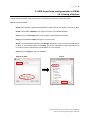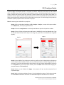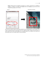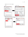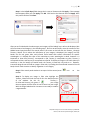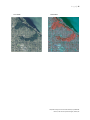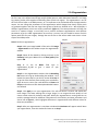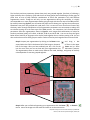
1
GEOSPATIAL CANOPY COVER ASSESSMENT WORKSHOP Software used: SPRING 5.1.7 and FRAGSTATS 3.3 Presented by: Dr. L. Monika Moskal & Dr. Diane Styers Computer Exercise Materials Developed by: Justin L. Kirsch Remote Sensing and Geospatial Analysis Laboratory Precision Forestry Cooperative at the School of Forest Resources University of Washington Page |2 Table of Contents 1. BACKGROUND .................................................................................................................................................. 3 1.1 Purpose and Objectives ...................................................................................................................... 5 1.2 Remote Sensing Concepts ................................................................................................................... 6 1.2.1 Object Based Image Analysis (OBIA & GEOBIA) ......................................................................... 10 1.2.2 Accuracy Assessment ................................................................................................................. 12 1.2.3 Landscape Metrics ..................................................................................................................... 14 1.2.4 Change Detection....................................................................................................................... 16 2. ANALYSIS ........................................................................................................................................................ 18 2.1 Installing SPRING ............................................................................................................................... 19 2.2 Installing FRAGSTATS ........................................................................................................................ 20 2.3 OBIA Project Setup and Segmentation in SPRING ............................................................................ 21 2.3.1 Creating a Database ................................................................................................................... 21 2.3.2 Creating a Project....................................................................................................................... 22 2.3.3 Importing Imagery ..................................................................................................................... 24 2.3.4 Segmentation ............................................................................................................................. 28 2.4 OBIA Classification in SPRING ........................................................................................................... 31 2.5 Post Classification Analysis in SPRING .............................................................................................. 36 2.6 Exporting Imagery from SPRING ....................................................................................................... 38 2.7 Calculating Landscape Metrics with FRAGSTATS .............................................................................. 39 3. REPORTING..................................................................................................................................................... 45 4. CONCLUSION .................................................................................................................................................. 48 5. OTHER RESOURCES ........................................................................................................................................ 49 6. REFERENCES ................................................................................................................................................... 50 APPENDIX A: Data Sources................................................................................................................................. 52 APPENDIX B: Aerial Photography and NAIP ....................................................................................................... 53 APPENDIX C: Satellite Data Pre-Processing........................................................................................................ 54 APPENDIX D: Concepts and Definitions ............................................................................................................. 55 APPENDIX E: Accuracy Assessment Statistics .................................................................................................... 56 APPENDIX F: Landscape Metrics Descriptions ................................................................................................... 57 APPENDIX G: Future Readings ........................................................................................................................... 58 Geospatial Canopy Cover Assessment Workshop by UW RSGAL March 3, 2011 University of Washington, Seattle, WA Page |3 1. BACKGROUND With over 3.4 million residents (U.S. Census Bureau, 2010), the Seattle-Tacoma-Bellevue area is experiencing rapid population growth due to economic expansion in leading industries such as aerospace, biotechnology, information technology and international trade (City of Seattle, 2010). To meet the infrastructure needs of this growing population, forested and agricultural lands are being converted to human-modified urban uses at staggering rates. For example, increases in military and civilian personnel and their families due to growth at Joint Base Lewis McChord has resulted in a 201% population increase in the nearby City of DuPont since 2000 (U.S. Census Bureau, 2010). A visual scan of historical and current aerial photographs below quickly reveals a substantial amount of land conversion from natural cover to urban development west of DuPont to the Nisqually Delta. 1990 2007 Although historical aerial photography has been available for over 60 years, due to improvements in image processing tools it is just now rapidly evolving as a management tool (Morgan et al. 2010). Land cover and land use classes, such as forest canopy and impervious areas can be automatically classified and extracted from high resolution aerial and satellite imagery using new Geographic Object Based Image Analysis (GEOBIA/OBIA) techniques (Hey and Castilia 2008). Quantifying changes in cover using landscape pattern metrics, such as forest patch size and connectivity, helps us identify and visualize areas that are changing quickly (Dunbar and Moskal, 2004). This information can assist decision-makers with allocating funds and resources to areas that have been negatively impacted from development and need the most attention to prevent further canopy cover loss. Remote sensing technologies can provide a means to explore a variety of continuous environmental variables over large areas including canopy cover and other land use/land cover types. Remote assessments are reasonably simple and can be conducted quickly, inexpensively, and without access or disturbance issues encountered in ground-based data collections. These assessments provide a means to measure and monitor complex urban environments, and their dynamic ecologies. For instance, canopy cover surveys and forest pattern metrics are useful to help a city quantify current tree cover status (Hunsinger & Moskal, 2005), determine the locations and drivers of canopy loss or gain (Turner & Gardner 1991), and monitor these trends over time (Moskal et al. 2004). These data can then be used to select inventory sampling sites, establish tree protection requirements for new developments, assist with urban forest health management, and determine target areas for planting projects. Remote sensing techniques can be applied to the analysis of other human and environmental dynamics within urban systems to aid in sustainable planning and management of these areas. Geospatial Canopy Cover Assessment Workshop by UW RSGAL March 3, 2011 University of Washington, Seattle, WA Page |4 Outreach is essential to maintaining close ties with individuals and communities, sharing knowledge to inform decision‐making, and in turn, listening to questions, concerns, and feedback regarding their needs. The Remote Sensing and Geospatial Analysis Laboratory (RSGAL) is an applied science research laboratory meaning that analysis techniques developed by the lab are applied to real world issues through pilot studies, hands‐on workshops, and presentations to community focus groups. Through this free workshop, we aim to educate personnel of small local government and public organizations, who are an under‐represented audience in the field of remote sensing technologies, in hopes of providing innovative, time‐ and cost‐efficient approaches to sustainable urban management. The target audience is urban foresters, city planners, parks personnel, etc who are interested in learning more about their city’s forest resources but who don’t have the budget to do so. Each workshop attendee will receive training in one of the most technologically advanced image analysis techniques, which is valuable for both critically evaluating subcontracted work or conducting your own assessments, now and in the future. Geospatial Canopy Cover Assessment Workshop by UW RSGAL March 3, 2011 University of Washington, Seattle, WA Page |5 1.1 Purpose and Objectives Successful management strategies require a base of knowledge and information about forest resources in order to develop action plans and establish long-term goals. The mission of the University of Washington (UW) Precision Forestry Cooperative (PFC) is to develop advanced technologies to improve the quality and reliability of information needed for planning, implementation, and monitoring of natural resource management, to ensure sustainable forest management, and to increase the competitiveness of Washington's forest sector. As part of PFC, the Remote Sensing and Geospatial Analysis Laboratory (RSGAL) aims to provide a research rich environment and exceptional resources that drive scientific investigations of multi-scale dynamics of landscape change through innovative applications of remote sensing and geospatial tools, and promotes a transdisciplinary approach for sustainable management solutions to pressing environmental issues. Consistent with these missions, the main purpose of this project is to provide guided analytical training to urban foresters, land managers, and city planners in an innovative technique to quantify tree canopy cover using high-resolution aerial imagery, calculate forest change metrics, and select sampling sites for ground-based tree inventories. The benefit of undergoing such training is the ability to deliver the results from the report produced in the workshop with confidence and authority for advocacy purposes. Participants will be provided with: 1) Preprocessed sample imagery (2009 NAIP). 2) An accurate technique for analyzing these data that is repeatable on future dates, other locations, or other datasets (e.g., canopy cover, impervious surfaces, agriculture, land use land cover classifications). 3) Skills in quantifying and assessing the accuracy of the technique and how results can be used to develop a field sampling regime for more in-depth canopy assessment. 4) Skills in producing and understanding landscape metrics for multi-temporal change analysis. 5) Understanding of how the products can be used as the 1st step in land use, land cover mapping. 6) A summary report of their findings. This workshop module (description of method, training exercise, and report template) will then be freely available online to the general public. This workshop fills a need for city and county personnel in the state of Washington, who may not otherwise be able to afford training in the use of these new technologies in order to protect natural resources in their communities. After the workshop Dr. Moskal and Dr. Styers will work on a revision to the protocol based on the feedback provided by the workshop participants. The report will be on the project website hosted by RSGAL along with revised workshop manual and module at: http://depts.washington.edu/rsgalwrk/canopy/ To the right is a conceptual flow diagram of the process described in this workshop. Geospatial Canopy Cover Assessment Workshop by UW RSGAL March 3, 2011 University of Washington, Seattle, WA Page |6 1.2 Remote Sensing Concepts Remote sensing is the science of obtaining information about an area through the analysis of data acquired by a device that is not in contact with the area (Lillesand 2008). This typically involves imagery acquired through aerial photography or by sensors located on satellites orbiting the Earth. The process from data acquisition to presentation of results to stakeholders involves many steps, where a vast majority of time is dedicated to interpretation and analysis. Data Digital imagery must form the basis for the development of remote sensing products to guarantee data consistency and the understandable application of scientific methods. Ancillary data from field observations, vegetation and forestry maps, photos, and other records are also important sources of information for image classification and verification. Remotely sensed data is not always free; however some free sources include the National Agricultural Imagery Program (NAIP), which has been collecting nationwide aerial photography for decades. Some older aerial photographs can also be acquired from USGS at no cost and range as far back at 1930’s. NAIP imagery was acquired in black and white up until the 1980’s, true color was then acquired up until about 2000, and presently near-infrared false color imagery is typically flown. It is the near-infrared color imagery that is more suitable for vegetation studies as vegetation vigor is prominent in the near infrared region of the spectrum. Example of black and white (monochromatic), true color and near-infrared imagery, note the differences between vegetation and water in these types of image. More information about NAIP imagery can be found in Appendix B. For about a decade now LiDAR has been flow commercially and consortia have established regionally (Puget Sound LiDAR Consortium) and national (USGS Click). Unfortunately, LiDAR is not currently collected by a nationwide program at a yearly temporal interval, and some regions still do not have LiDAR coverage, while others have audited coverage due to the quickly changing technologies. One should remember that even older LiDAR data can provide very useful data, for example the 3D point cloud can be processed to extract a surface model which can then be used to produce a DEM. Canopy models and building models have also been attempted and are very useful inputs for remote sensing analysis. More information on LiDAR can be obtained on the RSGAL LiDAR workshop website at: http://depts.washington.edu/rsgalwrk/lidar/. Geospatial Canopy Cover Assessment Workshop by UW RSGAL March 3, 2011 University of Washington, Seattle, WA Page |7 Another source of free data for monitoring large areas such as counties and states is the digital satellite imagery of Landsat TM. Although comparatively low spatial resolution (30 m/pixel), Landsat data have been available since 1972. The level of spatial detail is too coarse for extracting information at the forest stand or sample plot (10 x 10 m) level. However, the Landsat TM data does give information on the larger landscape context, which can have impacts on local forest health. Furthermore, because of a slightly higher temporal resolution, Landsat data can show multiple inter-annual observations for a location; however, this ability is reduced in the Pacific Northwest due to cloud cover. For preprocessing imagery and extracting ground information useful in classification, another required source of data is the digital elevation model (DEM). Digital elevation data is similar to imagery except that each pixel contains a height value instead of a gray level intensity. Continuous coverage DEM data are available through base mapping programs, such as the Shuttle Radar Topography Mission (SRTM) which offers freely available data nationwide at 30 m per pixel resolution. Data pre-Processing Aerial and satellite remotely sensed data undergoes an extensive pre-processing prior to utilization, and although a majority of this work is done by the data providers, it’s critical to understand some of these concepts as these can have an impact on the accuracy of output products. Below we focus mainly on pre-processing of aerial data. However, as more and more high spatial resolution data sets are available from space borne sensors, it is important to be aware of the processes involved in generating these data. Satellite pre-processing is even more extensive and is discussed in more detail in Appendix C. Topographic Corrections If the slope of the study area exceeds a certain value (usually about 25 degrees), then a topographic correction is required in order to accurately classify imagery. Topographic slope and aspect can contribute to distortions in remotely sensed data. This is particularly true in mountainous areas completely shadowed by terrain, where the region of interest may be blocked from receiving solar irradiance. Requiring a DEM as input, topographic slope-aspect corrections aim to compensate for differences in pixel values that are due to the object’s orientation to the sun’s position, rather than to the reflectance properties of the objects on the ground. The amount of solar light that each pixel theoretically receives is calculated from the DEM, which is modeled to determine the brightness value to add or subtract from the original brightness values of the image. For surface normalization, simple cosine corrections have shown improvements to classification accuracy (Franklin 1991; Franklin and Giles 1995; and Dymond 1992). However, both over-corrections and under-corrections occur using these simple cosine models (Civco 1989). Although the sun-to-sensor angle is corrected to that of a flat terrain, differences in tree canopy shadow due to slope and aspect are not taken into account. More advanced methods of correction have been developed that model the relative position of trees and the amount of shadowing based on slope and aspect (Gu and Gillespie 1998) or that model the mixture of sun lit crown, shadowed crown, and background within a pixel (Li and Strahler 1985; Woodcock et al. 1994). Aerial topography can be corrected using DEM’s produced from stereo photo pairs using photogrammetric techniques, while some also rely on the above mentioned SRTM data. However, one needs to be careful when using a coarser resolution dataset for topographic corrections especially in heterogeneous areas such as urban landscapes. In these cases LiDAR is becoming the more appropriate source of DEMs. Geospatial Canopy Cover Assessment Workshop by UW RSGAL March 3, 2011 University of Washington, Seattle, WA Page |8 Geometric corrections, Orthorectification and Mosaicking During the process of acquiring digital imagery, geometric distortions occur due to variations in the sensor’s platform, the earth’s curvature, relief, and so forth. The company that supplies imagery frequently corrects systematic distortions in house or provides the values of variables for use with correction algorithms. Ground control points (GCP’s), or accurately located ground features that are identifiable on the image, are useful for correcting random geometric distortions. Distortions in scale occur because the distance between the sensor and the earth surface varies with elevation. To compensate for distortions in the flat surface of an image caused by being captured from an uneven surface of the earth, an orthogonal rectification is performed. Orthorectification is a mathematical manipulation in the locations of pixels of an image to the actual locations and elevations of certain known features on the ground. Mathematical models for orthorectification include nearest neighbor re-sampling, bilinear interpolation, and cubic convolution. Information regarding surface elevation is obtained using a DEM. Furthermore, imagery is often acquired as independent photos covering limited area, mosaicking of imagery is often down at the same processing step as orthorectification. One key step that needs skilled image analysis is matching the color or shading of imagery during mosaicking. The process is often referred to as histogram matching and it aims to eliminate tone differences between images. Cut-lines are often employed to stitch data sets along natural seams such as roads, water bodies or other linear features. Land use land cover (LULC) Land cover describes natural and built objects covering the land surface, while land use documents human uses of the landscape. Remote sensing imagery captures characteristics of the Earth’s surface, but it takes an interpreter’s knowledge about shape, texture, patterns, and site context to derive information about land use activities from information about land cover. LULC classifications typically utilize some modification of the Anderson hierarchical system, with generalized LULC classes described at Levels I & II and more detailed classifications for Levels III & beyond. Classification and Mapping For monitoring the forest landscape over time, conceptually simple and practically similar approaches to classification of digital data is required across the sample design. The databases used for detecting changes must be as consistently and accurately mapped as possible in order to avoid errors in accuracy. Often categorized as supervised and unsupervised, several approaches for multispectral image classification (Lillesand and Kiefer 1994) are available in standard image analytic software packages. Intermediate between these two are a series of modified approaches which attempt to capitalize on the strengths of the supervised and the unsupervised methods in a single procedure. One of the critical issues that must be addressed, after selecting the broad approach, is the choice of algorithm (statistical, non-parametric, fuzzy logic, evidential reasoning, neural nets, others). Geospatial Canopy Cover Assessment Workshop by UW RSGAL March 3, 2011 University of Washington, Seattle, WA Page |9 Supervised Classification A supervised classification utilizes the analyst’s knowledge of features on the ground. Mathematical algorithms use the spectral properties of known ground features (training sets) to determine the class identity of unknown image pixels. Unsupervised Classification An unsupervised classification uses clustering algorithms to distinguish pixels sharing similar spectral characteristics. The relationship of the resulting spectral clusters to ground features is subsequently identified. Per-Pixel Classification Traditional classification methods have used Landsat satellite imagery (inset a in figure below) to produce LULC maps (e.g., 2001 National Land Cover Database) by assigning individual pixels to a specific class based on spectral signature (inset c in figure below). The spatial resolution of this imagery is 30m, meaning that anything on the ground less than 30m in size, or 900m2 (9,688ft2) will be generalized to the main class represented in that pixel. 9,688ft2 is larger than most parcels in Seattle so detail beyond Anderson Level I or II cannot be obtained. It is now a well-accepted principle that this moderate resolution is not appropriate for LULC mapping in urban areas. Geospatial Canopy Cover Assessment Workshop by UW RSGAL March 3, 2011 University of Washington, Seattle, WA P a g e | 10 1.2.1 Object Based Image Analysis (OBIA & GEOBIA) A new classification method called Object Based Image Analysis (OBIA) appears to work best on highresolution satellite and aerial imagery as well as LiDAR data (e.g., 1m NAIP; Figs. 1b & 2). This form of feature extraction allows for use of additional variables such as shape, texture, and contextual relationships to classify features (Fig 1d). This method can be used on free publiclyavailable high-resolution nationwide NAIP imagery, which can be classified at Anderson Level III and higher to achieve very detailed LULC maps for urban-based planning, management, and scientific research. To the left is a comparison between a Landsat 30m pixel resolution image (a) classified using per-pixel method (c), and a National Agricultural Imagery Program (NAIP) 1m pixel resolution image (b) classified using Object Based Image Analysis method (d). Note the higher image detail in the OBIA classification and the greater number of classes possible. Geographic object based image analysis (GEOBIA) is a method of classification involving the delineation (segmentation) of similar pixels into discrete objects and is followed by the classification of those objects into themes or classes. An assumption of GEOBIA is that the landscape is made up of homogenous patches which can be separated by their spectral signatures. The simplest and longest standing approach to image classification in remote sensing is the per-pixel based supervised and unsupervised classifications. The per-pixel classification categorizes remotely sensed image pixels by a theme, such as land cover. The classification uses the numerical data of spectral information contained within each pixel as the basis for this categorization (Lillesand and Kiefer, 2000). The user then has the ability to select the classification algorithm (or decision rule) based on the nature of their input data and their desired results. The algorithm or decision rule determines the manner in which pixels are assigned to categories by evaluating each pixel’s spectral information and the spectral information of its neighbors. Types of decision rules include parallelpiped, minimum distance, and maximum likelihood classifiers (Jensen, 1996). Feature extraction classification is an object-oriented approach to image classification. Feature extraction uses relationships such as size, shape, texture, directionality, repetition, context, as well as spectral information to categorize pixels (Lillesand and Kiefer, 2000). Both object-oriented and per-pixel Geospatial Canopy Cover Assessment Workshop by UW RSGAL March 3, 2011 University of Washington, Seattle, WA P a g e | 11 classifications look at signatures to aid in categorizing pixels. However, the per-pixel classifications only have spectral information signatures. Object-oriented techniques also produce signatures, but for a much larger set of information, including the above-mentioned characteristics such as size, orientation, texture, etc. Along with a more robust set of signatures to aid in more accurate pixel categorization, object-oriented approaches also look at the relationship of signatures among neighboring objects (Cothren and Gorham, 2005). Object-oriented feature extraction using Feature Analyst provides a multidimensional approach to image classification, making more efficient use of the depth of information contained in an image. Most importantly, the incorporation of spatial relationships and the scaling of objects incorporate the fundamentals of geography and landscape ecology into image classification techniques. Applying geographical concepts to image classification techniques most often provides superior results more reminiscent of the natural landscape compared to traditional per-pixel methods (Blaschke and Strobl, 2001). Fundamentally, classifications generated under the consideration of spatial relationships are consistent with using landscape metrics, which also use the premise of spatial relationships and scale to describe the resulting classifications. Geospatial Canopy Cover Assessment Workshop by UW RSGAL March 3, 2011 University of Washington, Seattle, WA P a g e | 12 1.2.2 Accuracy Assessment Performing an accuracy assessment on the classification results is mandatory in order to evaluate the truthfulness of the classified thematic map’s representation of real world attributes (Congalton and Green, 1998). An appropriately designed accuracy assessment compares not only the classification map, but also the ground reference test information, and to what degree the classifications represented thematically are actually correct to the corresponding ground reference locations (Jensen, 1996). However, when land use/land cover classification procedures are performed on historical aerial photography, ground reference test information current to the date of image capture cannot be obtained to validate the classification for historic dates. If land use/land cover classifications had previously been generated for the location, those could serve as possible reference data for the accuracy assessment. However, lacking previous land use/land cover classifications for comparison, the accuracy assessment can also be performed by using a skilled air photo interpreter to verify the classification results with the source image (Skirvin et al., 2004). Workstation Assessment The skilled air photo interpreter assessments can be performed at the workstation. A workstation assessment involves randomly selecting multiple locations on the land use/land cover classification, noting its class assignment, and comparing it to its actual (interpreted) land use/land cover as determined from the image. Random points can be generated using an extension to ArcGIS called Hawth’s Spatial Ecology Tools > Generate Random Points tool (http://www.spatialecology.com/). Hawth’s Tools is an open source extension for ESRI ArcGIS. Hawth’s tools is designed to perform ecology related spatial analysis. It is a useful tool to aid in sampling design, allowing for a variety of sampling techniques (stratified random sampling, grid sampling, polygon sampling). Field Validation Protocols for collecting field data will vary according to the classification and change detection methods employed. In general there would be a requirement for field data to train the classifier and verify the accuracy of classification; then, a separate field data set would be required to focus on the changes in classification that are revealed by the multitemporal change detection analysis. In the case of unsupervised classification, minimal field data are required initially, although the biological context would be difficult to generate without access to field observations – in essence, a field program to label the clusters would be required in subsequent years. In the supervised and modified supervised approaches a significant field program is required to develop and implement the classification in the first year and in subsequent years the field program would be aimed specifically at areas of change. For example the figure shows a random two-phase stratified sample for Seattle, first stratified by sampling region then by zoning. Geospatial Canopy Cover Assessment Workshop by UW RSGAL March 3, 2011 University of Washington, Seattle, WA P a g e | 13 1.2.2.2 Error or Confusion Matrix Beyond providing an average classification accuracy, remote sensing data should always include an error or confusion matrix, this matrix can help one assess per class accuracies. This is particularly useful when we are only interested in one class form the LULC classification such as forest canopy. For example the overall classification might be 85%, but often canopy classes have lower accuracies, which are lost when only the overall accuracy is reported. The matrix also helps the analyst to determine if the algorithm and data sets performed well (producer accuracy), often the algorithm is revised after exploring initial accuracy assessments. The end map user should be mostly concerned with the users accuracy, as it lets them know the type of accuracies to expect on the ground, but a check of the producer’s accuracy can help to determine in the most appropriate methods were used while discussing this with the analyst. The structure of the error matrix allows for the production of overall accuracy of the entire classification, and a producer’s accuracy and user’s accuracy for each class. All three of these values should be reported, since the future use of the classification is unknown (Felix and Binney, 1989). Below is an example of an Error or confusion matrix which can be based on field validation, auxiliary data validation, or even visual interpretation of remotely send data. Visually Interpreted Impervious Forest Background Matrix Total Errors.of Commission Impervious A Q W J A/J Forest Background Matrix B R X K R/K C S Y L Y/L Total Errors.of Omission D T Z n A/D R/T Y/Z Classified Class Overall Classification Accuracy A+R+Y/n The overall accuracy is calculated by dividing the number of correctly classified locations by the total number of locations assessed for accuracy (n = 100). The correctly classified locations are those on the diagonal within the matrix (A, R, Y) (Story and Congalton, 1986). The errors of commission, those that yield the user’s accuracy, are found in a column on the right side. These values represent that the classification algorithm generated “J” number locations to a specific land use/land cover class. Only “A” number of those locations were an instance of correct class assignment (Q + W committed, omitted from their correct class). A/J generates the probability that a pixel classified on the map actually represents that category on the ground (Story and Congalton, 1986). The errors of omission, those that yield the producer’s accuracy, are found in a row at the bottom. These values represent that within that year’s study area, there were “D” number of instances of validation locations within that land use/land cover class column. “A” number of those locations were actually produced as such class (with B + C omitted, committed to other classes). A/D generates the probability of a reference pixel being correctly classified (Story and Congalton, 1986). Geospatial Canopy Cover Assessment Workshop by UW RSGAL March 3, 2011 University of Washington, Seattle, WA P a g e | 14 1.2.3 Landscape Metrics Landscape metrics quantify the composition and pattern of patches in the landscape and can be categorized according to their general function in the table below. In addition to simple description of the landscape, certain metrics attempt to measure aspects of landscape pattern thought to reflect or influence underlying ecological processes. In most cases, however, the relationships between landscape metrics and biological phenomena have not been validated with field studies. Validation of landscape metrics with biological phenomena is particularly complicated when targeting a wide phylogenetic range of taxa, such as aimed for in a biodiversity monitoring program, because patterns of the landscape may affect various organisms differently. Readily available landscape analytical programs such as FRAGSTATS (McGarigal and Marks 1994) and Patch Analyst (Elkie et al. 1999) can be used to calculate a large number of metrics for the landscape patches derived from a classification of remotely sensed imagery. Since an overwhelming number of metrics are described in the literature, the choice of appropriate sets of landscape metrics must be based on criteria meaningful to the program at hand. Monitoring forest biodiversity requires that landscapes be compared, temporal changes be evaluated and possibly that landscape effects be predicted. The criteria for selecting metrics should include: • • • • Simplicity of interpretation Simplicity of mathematics Low correlation (statistical independence) among the set of metrics Relevance as disturbance (fragmentation) indicator Geospatial Canopy Cover Assessment Workshop by UW RSGAL March 3, 2011 University of Washington, Seattle, WA P a g e | 15 According to Jaeger (2000), “fragmentation measures should 1) increase monotonously when new sites are converted into intensively used areas, e. g. into settlement areas and roads; 2) have an intuitive explanation; 3) not be too sensitive to the omission or addition of very small residuals: 4) not require much data input; 5) be as simple as possible from a mathematical point of view”. New metrics and empirical data supporting the interpretation of metrics relative to ecological criteria continue to be introduced in the literature at a high rate. According to Simberloff (1999) the most critical issue facing landscape ecologists is the verification of the ecological relevance and meaning of landscape metrics. Based on this literature review we recommend metrics in Appendix F. Landscape Scale It serves well to identify the scale level at which the relationship between structure, function, and change can most accurately explain the landscape dynamic at hand. Landscape metrics deal in three levels of scale: landscape, class, and patch (Forman and Godron, 1986). The smallest unit in a landscape is the patch. A patch is a relatively homogenous nonlinear area that differs from its surroundings (Forman, 1995). Metrics for this scale contain information for every individual patch, regarding its spatial character, as well as measures of deviation from other patches within the same class and patches from other classes within the landscape. An assemblage of patches based on a common attribute, such as land use/land cover type, constitutes a class. Class metrics summarize the overall spatial character of all patches within the class as well as the composition and spatial configuration of the class. An assemblage of classes (and their respective patches) constitutes a landscape mosaic (Fragstats, 2002). Geospatial Canopy Cover Assessment Workshop by UW RSGAL March 3, 2011 University of Washington, Seattle, WA P a g e | 16 1.2.4 Change Detection A number of approaches for change detection using remotely sensed multi-temporal data sets are described in the literature (see Lillesand and Kiefer 1994; Jensen 1996). In general, to reduce the need for image calibration, if possible, image parameters should remain constant, i. e. the same time of year, time of day, spectral bands, sensor, sensor look angle, spatial resolution, and so forth. Imagery with obvious features that can be confused with change, such as clouds or extreme soil moisture conditions, should be avoided. Images to be compared must be carefully geo-rectified and registered to the same map projection to avoid mistaking misregistration for change. An assumption for all change detection techniques is that the areal extent of the changes to be detected is larger than the spatial resolution of the imagery. To detect rapid changes to the environment such as residential development, a short time span sequence of images is required, whereas to detect trends and to forecast, a longer time span and larger number of images is required (Hame et al. 1998). Visual Change Detection For qualitative assessment and display purposes, changes can be visualized by loading corresponding bands from multi-date images into different computer display channels. No change, positive change and negative change appear as different colors in the image, useful for a general examination of land cover change. However, the composition and quantity of change cannot be identified or calculated from the visual change detection method. Direct Multi-Date Classification or Post-classification Analysis The direct multi-date classification approach involves independent classifications of imagery from different dates being compared to detect changes in the landscape. One advantage of this method is that absolute calibration of the imagery is not required if the changes are prominent or if good ground data for training sets are available. Disadvantages are that errors in classification may be compounded in the change detection analysis, resulting in a misinterpretation of change. Supervised classification First, independent supervised classifications using imagery from different dates are produced of the study area. A matrix can then be made which compares the classifications on a pixel by pixel basis, allowing to and from analysis of change. Unsupervised classification A disadvantage to many methods that rely on supervised classification is the need for high quality training data, often not available for change detection studies. Unsupervised classification, which does not require training data, is sometimes combined with other methods for change detection (see Combination of Analyses section). Geospatial Canopy Cover Assessment Workshop by UW RSGAL March 3, 2011 University of Washington, Seattle, WA P a g e | 17 Classification of Multi-temporal Data Sets Data sets composed of imagery from more than one date are combined and classified using either a supervised or unsupervised approach. This method is only successful if the spectral value of the change classes differs significantly from the unchanged classes. Problems associated with this method include labeling the change classes and identifying how classes have changed. One procedure is simply to combine image bands from multiple dates, produce an unsupervised classification and label the clusters as changed or unchanged. Alternatively, Principal Components Analysis (PCA) or Tasseled Cap Transformation can be used on the combined data set, which produces a new de-correlated data set (Eastman 1992). One or more of the resulting data channels correspond to the differences (change) between the original two temporal images. Image Algebra Image subtraction: The digital values from one image date are subtracted from the values of another date. Areas with change will have large differences in value, while those with little change will have small differences Image ratio: A ratio of the band of one image date to the band of another image date is created. For areas with no change, the value of the ratio tends toward one. Areas of change will deviate to higher or lower ratio values. How much deviation is required for change is based on selected threshold values. Change Vector Analysis The magnitude and direction of spectral change between two image dates can be obtained by plotting for single pixels, the values for two spectral variables for the two dates. The magnitude of the change is the Euclidean distance between the two points. The direction of the vector relates to whether the change is positive or negative. For example, a negative change might be a loss of vegetation whereas a positive change might represent vegetative re-growth. Combination of Analyses Traditional classification of a reference image to develop base classes can be combined with information derived from a change image. To extract information on the classes that have changed in the second image, only the area under the binary mask need then be classified. By limiting the second classification to areas of change, the classification requirements are not as complicated. Geospatial Canopy Cover Assessment Workshop by UW RSGAL March 3, 2011 University of Washington, Seattle, WA P a g e | 18 2. ANALYSIS Geospatial Software A wide range of geospatial software is available commercially, as freeware and as open source. Segmentation is an analysis imbedded in the following image analysis software: ENVI, ERDAS Imagine and IDRISI. OBIA based classifications are possible as extension software to ERDAS and ARCGIS called Feature Analyst or as standalone packages: Berkeley Image Segmentation and Definiens eCognition. The cost of these packages can be prohibitive, with eCognition toppling the cost scale. We chose freely available software for this workshop, although there are pros and cons to using freeware, we believe cost is often the most limiting factor, thus, we hope that the detailed steps presented in this workbook help to overcome some of the downfalls of the freeware. The following two free software packages will be demonstrated in the applied section of this workshop: 1) SPRING http://www.dpi.inpe.br/spring/english/ SPRING is a freely available product of Brazil's National Institute for Space Research (INPE) and is a state-of-the-art GIS and remote sensing image processing system with an object-oriented data model which provides for the integration of raster and vector data representations in a single environment 2) FRAGSTATS http://www.umass.edu/landeco/research/fragstats/fragstats.html FRAGSTATS is a computer software program designed to compute a wide variety of landscape metrics for categorical map patterns Geospatial Canopy Cover Assessment Workshop by UW RSGAL March 3, 2011 University of Washington, Seattle, WA P a g e | 19 2.1 Installing SPRING SPRING is a freely available object-oriented remote sensing software package used for image processing of both raster and vector data. It allows the user to automatically classify imagery, which groups together similar pixels in an image into land cover classes or themes. This workshop is aimed at providing an accurate and repeatable technique for extracting canopy cover from imagery and analyzing its change over time. After installation of both SPRING and FRAGSTATS (section 2.1b) we will focus on calculating canopy cover for an area of Tacoma using imagery from 2009. Task 1: Install SPRING 5.1.7 Step A: Step A: Navigate to the SPRING website (Ctrl + left click on the following link: http://www.dpi.inpe.br/spring/english/index.html. Install the SPRING 5.1.7 software package by clicking on Download in the upper left. Step B: To register your copy of SPRING enter your email address, a password, and choose the SPRING for Windows 32 version from the Version drop down list (while SPRING offers a 64 bit version, the SPRING software performs optimally in a 32 bit atmosphere). Step C: Choose ‘install complete’ to install the SPRING, IMPIMA, SCARTA package in the English column and then click run. will now be added to your list of programs. Step C: SPRING Geospatial Canopy Cover Assessment Workshop by UW RSGAL March 3, 2011 University of Washington, Seattle, WA P a g e | 20 2.2 Installing FRAGSTATS In this section we will install the freely available program FRAGSTATS version 3.3. FRAGSTATS is a landscape ecology tool used to quantify landscape structure from data derived from imagery. It is provides the user with metrics to statistically describe a landscape. Task 2: Install FRAGSTATS 3.3: Spatial Pattern Analysis Program for Categorical Maps Step A: Navigate to the FRAGSTATS website (Ctrl + left click on the following link http://www.umass.edu/landeco/research/fragstats/fragstats.html. Step B: Click FRAGTSTATS Download in the left hand column. Step C: Double click the FragSetup33zip file and save it to the desktop. Step D: Unzip the folder on the desktop (right click and click Extract All… then click Extract). Step E: After the file has download there will be an unzipped folder named FragSetup33 on the desktop. Open the folder and double click on the Setup Application. FRAGSTATS will now be added to your list of programs. Step B: Step C: Geospatial Canopy Cover Assessment Workshop by UW RSGAL March 3, 2011 University of Washington, Seattle, WA P a g e | 21 2.3 OBIA Project Setup and Segmentation in SPRING 2.3.1 Creating a Database In order to work with data in SPRING you must first create a database. Databases are where all of your project folders are stored. Here we will create our database and define its spatial projection. Task 3: Create a database Step A: Open SPRING, a window titled ‘SPRING 5.1 New Features’ will appear, close this window. Step B: Click on File – Database in the upper left corner of the SPRING window. Step C: Click on the Directory button and navigate to the Desktop and click OK. Step D: In the Databases Name field type in your last name. Step E: Choose a database type from the Manager drop down list, we recommend using Access or dbase as your database type. Click Create, you will be prompted to assign a password, click no unless you want a password for your database; it is not required. Step F: Now click Apply to load your database. Steps C, D, and E: Step C: Geospatial Canopy Cover Assessment Workshop by UW RSGAL March 3, 2011 University of Washington, Seattle, WA P a g e | 22 2.3.2 Creating a Project After creating a database you are now ready to create a project within your database. This is where all of your imagery and outputs specific to a project are stored. More than one project can be created within a database, but only one project can be viewed at a time. The following steps will cover how to create a project and will also cover how to define a spatial projection for your project area. While it is possible to create a project without spatial projection this is not recommended. One would still have to define a projection when exporting any file created within that project. To avoid doing this step later we will define a spatial projection when we create the project. Task 4: Create a project and define its projection Step A: With your database loaded go to File – Project…- Project…, to open the Project window. In the Name field, name your project Tacoma. Step B: Click on the Projection box in the Project window to open the Projections window. Step C: Click on UTM in the Systems box and Datum-> NAD83(US) in the Earth Models box. Type 10 into the Zone field and click away in the Long: box, (you will see coordinates for Longitude appear). Step B: Step C: Step D: In the middle of the Projections window you will see that the Hemisphere radio buttons are not active and are locked on South, this is a problem because we will be using North for our projection. To activate the Hemisphere radio buttons click on the Polar Stereographic projection in the Systems box, you will see them activate, click the North radio button then change your projection back to UTM NAD83(US). Step E: When you are finished click Apply. Your project will now use this projection for all imported images. Step F: With the Projects window still open, in the Bounding Box region of the Projects window click the Planes radio button and make sure both N Hemisphere radio buttons are selected. Geospatial Canopy Cover Assessment Workshop by UW RSGAL March 3, 2011 University of Washington, Seattle, WA P a g e | 23 Step G: Manually enter the following coordinates as is shown circled below: X1: 537888, X2: 539728, Y1: 5235270, Y2: 5237361. Click Create and then click Load (note: you will not see the image below-right after you click load). Step G: Visualization of Step G: You have just created a project with spatial projection and a bounding box for your project, which creates a maximum extent for the project area. If an imported image is larger than this box then all areas outside of this extent will be clipped out. The outlined region on the image at left visualizes the bounding box step; the rectangle represents the bounding box. Geospatial Canopy Cover Assessment Workshop by UW RSGAL March 3, 2011 University of Washington, Seattle, WA P a g e | 24 2.3.3 Importing Imagery Once a database and a project have been created the next step is to add imagery to a project. SPRING works best if imagery is imported using the same spatial projection as the project. It is a good idea to know the projection of your imagery before defining the projection of your project. For reference, the imagery we are using today is projected in UTM NAD 83 Zone 10 North, which is why this projection was used when defining the project projection. Task 5: Import Imagery Step A: With SPRING open click File – Import- Import Vectorial and Matrical data. Step B: Click the File box and navigate to the folder where the Tacoma.tif file is stored. Step C: In the File window change the file type from ASCII-SPRING (*.spr) to TIFF/ GEOTIFF (*.tif *.tiff) by clicking on the File of type dropdown list. The Tacoma.tif file will appear, click on the Tacoma.tif file and then click Open. Step B: Step C: Step D: After loading the Tacoma.tif file click the Bounding Box button to open the Bounding Box window. Step E: Click the Project and Planes radio buttons. If both Hemisphere S radio buttons are selected change them both to N. Step F: If there are decimal places after the X1, X2, Y1,and Y2 coordinates then click back and forth between the Active PI and Project, and Geographic and Planes radio buttons until they disappear. If this step was necessary then be sure to return your radio buttons back to Project and Planes. Geospatial Canopy Cover Assessment Workshop by UW RSGAL March 3, 2011 University of Washington, Seattle, WA P a g e | 25 Step G: When you are finished click Apply. Step D: Steps E, F, and G: Step H: With the Import window still open click the Output tab. Click the Category button and change the category to CAT_Image and click Apply. Geospatial Canopy Cover Assessment Workshop by UW RSGAL March 3, 2011 University of Washington, Seattle, WA P a g e | 26 Step I: In the IL (info layer) field change the IL name to Tacoma and click Apply. If the message below appears after you click Apply, click OK. Click back to the Data tab and click Apply. Once this process finishes click Close. After you are finished with the above steps your imagery will be loaded, but it will not be displayed. We will cover how to load imagery in the following steps , but first we will briefly cover the contents of the SPRING control panel window. The control panel is the screen on the left with the Tacoma_1 through Tacoma_4 bands. This is where the information of your imagery is displayed. Our imagery has four bands: one for red, green, blue, and infrared. These bands each contain information for specific wavelengths. It is beyond the scope of this workshop to cover wavelengths in detail, however it is important to know that Tacoma_1 corresponds to red, Tacoma_2 corresponds to green, Tacoma_3 corresponds to blue, and Tacoma_4 corresponds to infrared. To display an image in true color (what you would see in the real world) you would match the Tacoma_1 band with red, and so on. However, instead of doing this we will load our image in false color, by loading the infrared band instead of the red band, this will make it easier to identify vegetation in our imagery. Step J: If the control panel window is not open click the control panel toolbar. icon on the Step K: To display our image in false color highlight the Tacoma_4 band and check the box for R in the bottom portion of the window. Do this for Tacoma_2 for blue and Tacoma_3 for green. If your image does not appear click the Zoom IL icon to zoom into your image. With the image loaded and in view we are now ready to conduct a segmentation. Geospatial Canopy Cover Assessment Workshop by UW RSGAL March 3, 2011 University of Washington, Seattle, WA P a g e | 27 True Color: False Color: Geospatial Canopy Cover Assessment Workshop by UW RSGAL March 3, 2011 University of Washington, Seattle, WA P a g e | 28 2.3.4 Segmentation In this section we will perform a segmentation, sometimes referred to as a delineation. Segmentation is the first step in the object-based image analysis (OBIA) process, which delineates features in an image by grouping similar pixels together and dividing those pixels into regions. The segmentation is one of the most critical steps in the OBIA process, so it is important to be comfortable with the segmentation output. You can change the parameters of the segmentation which changes how closely similar pixels are grouped together and also how large those groups of pixels are allowed to be. We will display 4 different segmentations, which use various parameters (Figure 1). The same parameters will likely not work for 2 separate images, so one likely has to perform numerous segmentations with different parameters to get the ideal segmentation. No one way is correct, but you should be aware of which options work best for your imagery. Settings that are too fine or too coarse could create issues in later steps of the OBIA process. Step B: Task 6: Perform a segmentation Step A: With your image loaded in false color click Image – Segmentation on the toolbar to open the segmentation window. Step B: Select all four bands by clicking on them, in the Similarity field type in 30 and an in the Area (pixels) field type in 100. Step C: In the segmentation_30_100 segmentation. IL to Name give a filed type in name to your Step D: In the Segmentation window click the Bounding Box button to bring up the Bounding box window. Here repeat the same steps as you did on section 2.3c Step F to get rid of the decimal places trailing your coordinates. Again be sure to return your radio buttons to Planes and Project, and make sure both Hemisphere N radio buttons are selected. Step E: Click Apply to run your segmentation. This will take about 5 minutes and would take much longer if we were working with a larger image (i.e. an image with more pixels) or had chosen smaller values for similarity and pixels. While your segmentation is running take time to read the passage below for additional information on the Similarity and Area parameters and also to look at Figure 1., which highlights differences in segmentations with different values for these two parameters. Step F: After your segmentation is complete a window titled Assistant will appear and will draw your segmentation, close this window and move on to Step F. Geospatial Canopy Cover Assessment Workshop by UW RSGAL March 3, 2011 University of Washington, Seattle, WA P a g e | 29 The Similarity and Area parameters dictate how pixels are grouped together (Similarity of 10 being a higher similarity than a similarity of 30) and the size of those groups (Area of 40 being a smaller group of pixels than an area of 100). Different combinations of these two parameters will yield different segmentation results. Though we will only run one segmentation during this workshop, it is highly recommended to run many segmentations before going through with the next step of the OBIA process. By carefully examining Figure 1 you will notice that pixels are not always put in groups that make sense. Sometimes tree pixels are grouped with road pixels. This is a source of error that one will never fully eliminate, rather through manipulation of the segmentation parameters one can attempt to reduce this error before moving on to the later steps of the OBIA process. For comparison, let’s see how different parameters affect our segmentation. Shown in Figure 1 are 4 images with combinations of values for Similarity and Area (pixels) of 10 & 40, 10 & 100, 30 & 40, and 30 & 100. You can see from the figure below how a Similarity of 10 groups more similar pixels together than a similarity setting of 30. You can also see that that an Area of 40 groups a smaller number of similar pixels together than an Area of 100. Step G: Inspect your segmentation by clicking on the Zoom cursor and drag a box around either the field in the bottom left of the image or the patch of forest in the upper left of the image. After you have outlined your box click on the Draw tool to zoom into the area. Here you can see how well your segmentation has delineated features. The segmentation seems to make sense; features like roads, buildings, and groups of similarly colored patches of trees are grouped together. Step H: After you are finished inspecting your segmentation click the Reset tool to return the image to its full extent and move on to the next section. or Zoom IL Geospatial Canopy Cover Assessment Workshop by UW RSGAL March 3, 2011 University of Washington, Seattle, WA P a g e | 30 Figure 1 10_40 30_40 10_100 30_100 Geospatial Canopy Cover Assessment Workshop by UW RSGAL March 3, 2011 University of Washington, Seattle, WA P a g e | 31 2.4 OBIA Classification in SPRING After completing the segmentation you are now ready to begin the classification steps of the OBIA method. A classification uses the delineated pixels from the segmentation to automatically categorize pixels in an image into similar classes. You will first have to provide training data for the classification to work; more simply you have to tell SPRING what to call what. For example if you wanted to create a classification with 2 classes you would tell SPRING to call some pixels trees ‘trees’ and all other pixels ‘non-trees’. We will cover these steps in detail in the following section. Task 7: Context Creation and Classification Step A: Go to Image – Classification to open the Classification window. You do not need to click the Directory button, the classification will be stored to the same path as defined in earlier steps. Step B: Click the Create button to open the Context Creation window. This is where you will create a file for the classification. Step C: In the Context Creation window type in classification1 in the Name field and click the Regions radio button. Select all bands by clicking on them and click segmentation_30_100 in the Segmented Images box, then click Apply. A file for classification1 will be created. Step B: Step C: Step D: With the Classification window still open click on classification1 in the classifiaction1 active. Contexts box, this will make Geospatial Canopy Cover Assessment Workshop by UW RSGAL March 3, 2011 University of Washington, Seattle, WA P a g e | 32 Step E: With classification1 active click the Extraction of attributes of the regions button. This makes the classification boxes in the bottom of the Classification window active. Step F: After the Extraction of attributes of the regions process is complete click the Training button. A window will appear telling you to acquire sample(s), click OK. To perform a classification we first have to tell SPRING what groups of pixels belong to what features. For example, by looking at the segmentation we can see that like pixels are grouped together, for example tree canopies that are next to roads are separated by lines. During the training portion of the classification step we will provide names (classes) for groups of like pixels. This is called a supervised classification because the user is determining the number of classes and the pixels that belong in those classes. In other words the user tells SPRING what to call what. Step G: In the Training window type the name ‘water’ in the Name field and choose a blue color for water by clicking on the Color box, then click Create. You have just created a class for water. The name ‘water’ will appear in the Themes box with zero acquired pixels. You have just created a class named water which you will place regions of water pixels into by selecting them from the image. This is another crucial step in the OBIA method because it determines what pixels are going to be grouped into what classes. Now that we have a class for water we will have to acquire training samples for the water class. Step H: In the Training window make sure the Region radio button is selected. Zoom to some water in the image (you may have to click the Zoom IL icon on the toolbar first to display your image in full). Step I: Click the Cross Cursor on the toolbar if it is not already selected, then click some water in the upper right of the image. A group of pixels will be outlined in blue, with these pixels selected click Get in the Training window. Do this for 4 more regions of water pixels and then move onto Step G. Geospatial Canopy Cover Assessment Workshop by UW RSGAL March 3, 2011 University of Washington, Seattle, WA P a g e | 33 Step J: Repeat Steps D-F for the classes trees, roads, buildings (i.e impervious surfaces), and grass; create your classes in this exact order. Notice that in this false color image vegetation is red, this is because living vegetation reflects in the infrared wavelength, which gives it a red appearance. Also notice that the grass in the track in the lower left of the image is not red. This is because this is artificial turf and not actually grass, which absorbs infrared giving it a gray appearance. You would not want to acquire training samples for grass from this field. Step K: After acquiring all of your samples click Save and then click Close. Step L: With your training steps complete click the Classification button in the Classification window. In the Type of Classification drop down box (Tipo do Classificador) choose the Bhattacharya method. Step M: In the Acceptance Threshold drop down pick an acceptance threshold of 99.9 then click the Sample Analysis button. You can choose to save the output if you wish, but you do not have to. Click Close to close the Sample Analysis window. Step N: In the Name field name your classification classification1 and click the Classify button to run the classification. After the classification process is complete take some time to inspect the output. By comparing the true color image with your classification, you will be able to see that there are misclassified regions and regions that have not been classified at all. We will need to refine our classification by selecting new training data for our classes. This is okay, refining a classification can take a long time, however it is important to be comfortable with your classification before applying it to a larger data set. We will now try to refine this classification by selecting new training data for our classes (for reference misclassification is often caused by shadows). In the image below you can see that there are lot of water pixels too far inland. These are mostly shadows from tree canopies and buildings that are being placed into the water class because shadows and water are both dark. We will have to supply more training data to make these classes more accurate. We will fix these regions in the following steps. Geospatial Canopy Cover Assessment Workshop by UW RSGAL March 3, 2011 University of Washington, Seattle, WA P a g e | 34 Step O: Turn on segmentation_30_100 by highlighting it and then check the Labeled box in the bottom of the control panel. Turn classification1 on by highlighting it and then check Classified box in the control panel. Step P: Reopen the Training dialog box and make the trees Theme active by clicking on it. Click on some of the shadowed areas that have been misclassified as water, you can tell if they are water or not by looking at the true color image for reference. You can compare your classification with the true color image by toggling classification1 on and off by clicking the Classified box in the control panel. Step Q: With the trees class still active click on any region you think are trees but have been classified as something else. If necessary repeat these steps for any class that appears to need refining. When you are finished click Save and then click Close. Step R: Now open the Classification window and name the new classification classification2. Choose the same settings as you did in Step J and click the Classify button. You will be able to see that your classification will be improved, but not perfect. The region of canopy shadows that were being grouped into the water class are now being placed into the tree class. The classification of water has also been improved, in classification1 we can see that some water was being grouped into the roads and buildings classes. Also, we could have added a class for dry vegetation, for this image it would have made sense because it looks as though the image was taken in summer, as you can see by the mixture of brown and green grass. For this classification we have essentially grouped dry and green grass into one class. Needless to say this classification is not perfect. There are inevitably going to be areas that are misclassified or not classified at all, but we have reduced this error and it is recommended that one continues to refine a classification until they are reasonably happy with the output. For the purposes of this workshop we will stop refining the classification and use the output from classification2 for the next section. Geospatial Canopy Cover Assessment Workshop by UW RSGAL March 3, 2011 University of Washington, Seattle, WA P a g e | 35 Classification 1 Classification 2 Geospatial Canopy Cover Assessment Workshop by UW RSGAL March 3, 2011 University of Washington, Seattle, WA P a g e | 36 2.5 Post Classification Analysis in SPRING Post classification is a process that refines your classification and also places unclassified pixels into classes. It is highly recommended that one runs a post classification especially if there are a large number of unclassified pixels in the classification. Like refining your initial classification by acquiring more training data, post-classification can significantly improve the accuracy of your classification by refining your classes. Task 8: Perform a Post-Classification Step A: From the toolbar click Image – Classification and click on Post-classification in the Classification window. Step B: In the Post-Classification window click on classification2 and choose a Weight of 7 and a Threshold of 7, then click Apply. Step C: When the post-classification is complete rename it from classification_pos to classification_pos_7_7 by right clicking it clicking on Rename… then click OK to close the rename window Displayed in Figure 2 are two different post-classification with two sets of parameters for weight and threshold: one with a weight of 5 and a threshold of 2, and another with a weight of 7 and a threshold of 7. Notice that the original classification did not classify all pixels, you can see this in the upper left corner and middle of the image labeled none, a post-classification was not run on this image. Also notice that the dark line near the top portion track shows up in the 7_7 post-classification, but not the 5_2. Because this line might not actually be grass it appears that the 7_7 has misclassified these regions. It appears that the 5_2 post-classification has outperformed the 7_7, because of this we will choose the 5_2 parameters for use in later steps. Move onto section 2.6. Geospatial Canopy Cover Assessment Workshop by UW RSGAL March 3, 2011 University of Washington, Seattle, WA P a g e | 37 Figure 2 none 7_ 7 Figure 2. 5_ 2 7_ 7 Geospatial Canopy Cover Assessment Workshop by UW RSGAL March 3, 2011 University of Washington, Seattle, WA P a g e | 38 2.6 Exporting Imagery from SPRING Once we are comfortable with the output of our classification and post-classification, we are now ready to export the data for viewing in GIS or for use in the statistical analysis program FRAGSTATS. Task 9: Exporting your classification. Step A: In the control panel window highlight the classification_pos_7_7, then from the toolbar click File-Export-Export Vectorial and Matrical Data to bring up the Export window. Step B: In the Export window make sure that the format type is TIFF/GeoTIFF in the Format drop down box and click Save Step C: In the Save File window choose a folder to save your file into (we recommend using the same folder your database and imagery are stored in) and name the file classification2_pos_7_7 and click Save. When you are finished close the Export window and close SPRING. Step B: Step C: Step D: To view your classification and its properties, open ArcMap and start a new blank map. Step E: Use the Add Data button to add the classification2_pos_7_7 .tif file to your map, click OK when you are asked to ‘build pyramids’. Keep ArcMap open, we will use data from the classification2_pos_7_7 .tif Properties window in the next section. Geospatial Canopy Cover Assessment Workshop by UW RSGAL March 3, 2011 University of Washington, Seattle, WA P a g e | 39 2.7 Calculating Landscape Metrics with FRAGSTATS In this section we will run our statistics for canopy cover on our Tacoma imagery. We will use the classification2_pos_7_7 output to estimate percent canopy cover and the total area of canopy for our imagery. But first, for FRAGSTATS to make sense of our data we need to assign our pixels names which can then be attributed to our classes. For example, for our blue colored pixels to be called water we need to provide FRAGSTATS with information that connects the name water to blue pixels. We will use ArcMap and the Notepad program to do this. We will use the information in the Layer Properties window to create a .txt file which links pixels to names of classes. Task 10: Calculate tree canopy metrics using FRAGSTATS Step A: With ArcMap still open double click the classification2_pos_7_7 layer to bring up the Layer Properties window. Step B: In the Layer Properties window click the Symbology tab and click Unique Values in the Show field. ArcMap will ask you to build an attribute table, click OK. From here we can see what order our classes are in. This is important in creating the text file for our classes. Notice that there are 6 classes. The white class labeled 0 corresponds to unclassified pixels. For display, below we have changed the unclassified pixels to pink to easily identify them in our classification. In the count column we can see how many unclassified pixels there are. Some of these were classified in the post-classification, but not all of them. This is okay, there typically aren’t enough unclassified pixels to alter your statistics significantly. If there are then you would want to return acquire more training data and conduct another classification. Geospatial Canopy Cover Assessment Workshop by UW RSGAL March 3, 2011 University of Washington, Seattle, WA P a g e | 40 Step C: Here we will create a text file for our classes. Open Notepad, it should be in the Accessories folder. Step D: From the Layer Properties window in ArcMap we know the order of classes. Type in what you see at the right, with no spaces between characters (your class orders should be the same). This will tell FRAGSTATS how to order classes. Notice that the water class is the only one that is false, true. This means that we will not be factoring in water in our calculation of the total land area. This is important if you want to know how much of the land is taken up by canopy and do not want to factor in water as a percentage of the total area. Step E: When you finish entering in the list of classes click File- Save, and name the file Notepad file classes, save the file to the same folder your other data is stored in. Step F: With ArcMap still open double click the classification2_pos_7_7 layer to bring up the Layer Properties window. Click the Source tab. Under Raster Information look at the Columns and Rows values: Columns = 1840 and Rows = 2091. Keep note of these values, we will need them in the later steps. Step G: Open FRAGSTATS and Click File – New on the toolbar to create a new project. Step H: On the FRAGSTATS toolbar click File-Save to save your project. Navigate to the folder where your other data is stored, name the project Tacoma_canopy_metrics and click Save. Step I: From the toolbar click Fragstats- Set Run Parameters to open the Run parameters window. You can also get to the Run Parameters window by clicking the Set Run Parameters icon on the toolbar. Geospatial Canopy Cover Assessment Workshop by UW RSGAL March 3, 2011 University of Washington, Seattle, WA P a g e | 41 Step J: In the Run Parameters window fill out the Run Parameters as shown below: In the Input Data Type filed click the 8 Bit Binary radio button Click the 8-bit file name button and load the classification2_pos_7_7.tif file Click the Output File button and in the File Name field name your output Tacoma_canopy_metrics and click Open In the Grid Attributes box put in 1 for cell size, 999 for background value, and 2091 for number of Rows, and 1840 for number of Columns (circled below, this is the size of our imagery and is the information we obtained in the Layer Properties box in ArcMap) In the Class properties file field load the classes.txt file we created in Notepad In output statistics click the Class and Landscape metrics boxes After you are finished click OK and move onto the next step Geospatial Canopy Cover Assessment Workshop by UW RSGAL March 3, 2011 University of Washington, Seattle, WA P a g e | 42 Step K: Open the class metrics window by selecting the Class Metrics icon on FRAGSTATS toolbar. the Step L: Check the boxes for Total Area (CA/TA), Percentage of Landscape (PLAND), and Number of Patches (NP), then click OK. This tells FRAGSTATS to output only these class metric statistics. Step M: Open the landscape metrics dialog box by clicking the Landscape Metrics on the FRAGSTATS toolbar. Check the box for Total Area (CA/TA) to calculate the area of the image , then click OK. icon total Geospatial Canopy Cover Assessment Workshop by UW RSGAL March 3, 2011 University of Washington, Seattle, WA P a g e | 43 Step N: Click the Execute icon on statistics. the toolbar to run the process that calculates Step O: After the process is complete you should see the message below. Click OK and then click the Browse Results icon on the FRAGSTATS toolbar to bring up Results window. Step P: The results window will be blank, click the Class tab in the bottom left of the window to display the Class metrics statistics. Geospatial Canopy Cover Assessment Workshop by UW RSGAL March 3, 2011 University of Washington, Seattle, WA P a g e | 44 Step Q: Browse the results by clicking on the Class and Land tabs at the bottom left of the window. We can see from the PLAND (percentage of land) column in the Results window that the percentage of land taken up by canopy is about 26% (your results may vary and are determined by your segmentation parameters and your training data). In the Type column we can see our list of classes, note that water does not appear because we ‘turned it off’ in our Notepad text file. You may also see that there are some classes named with numbers, these are unclassified pixels that were not grouped into the unclassified class. Do not worry about these too much, there aren’t usually very many of them to affect your statistical output significantly. Congratulations! You have successfully calculated the percentage of canopy coverage for a 3 by 4 mile area in North Tacoma! This concludes the workshop on Conducting Canopy Cover Assessments using the freely available programs SPRING and FRAGSTATS. Geospatial Canopy Cover Assessment Workshop by UW RSGAL March 3, 2011 University of Washington, Seattle, WA P a g e | 45 3. REPORTING Lanscape metrics are often reported in tabular and graph formats. These reports are also supported by visualizations. For exmaple below are GEOBIA classificaiton results for two growing communities between the years of 1997 to 2004. The red color in the calssification represents impervious areas, the green forest canopy and the other color summarizes the background matrices (all other classes in the LULC classification). We can observe that in both landscapes the total area of the impervious class increases over time; however, it’s more difficult to distinguish changes in the forest class area. More improtantly we can observe for Landscape A the impervious areas in the 1990 image help to establish transportation corridors that serve as vectors for impervious area expansion near forested areas. However, the pattern is slightly different for Landscape B; the impervious areas increase, but the increase is centralized in the lower left hand corner. Again, it’s difficult to assess the change in area of the forest class for Landscape B. Although the visual products of GEOBIA LULC are powerful, detailed and informative, these do not provide us with numbers such as percent change in forest class or area increase in impervious class. The visual products of GEOBIA LULC classification often need to be supported with tabular and numerical reauslts. For example, FRAGSTATS allowed us to calculate many landscape metrics for these two landscapes for four different temporal observations. These calculations are reported in the graphs to the left. We only use few of the simplest landscape metrics: Area per Class, Number of Patches and Average Patch Size to report changes on the landscape. Thus our visual maps can be supported by numerical summaries. Here we see that Landscape A and B lost only little forest canopy over time, and in fact for Landscape B there is a slight increase in canopy from 1990 to 2003. We also observe the dramatic increase of impervious areas; that is consistent with our visual interpretation of the output maps. What the graphs cannot tell us is the spatial associations between impervious areas developing along linear corridors in Landscape A Geospatial Canopy Cover Assessment Workshop by UW RSGAL March 3, 2011 University of Washington, Seattle, WA P a g e | 46 and clustering of these areas in Landscape B. On the other hand what was difficult to visually observe on the maps, in terms of the changes in forest canopy cover is now clearly demonstrated by the Average Patch Area metirc. Over time the forests are becoming fragmented; this is true and consistent for both landscapes. We also observe that the Average number of impervious patches is decreasing over time, and the Average Patch Area metric informs us that the impervious patches are getting larger in size. This tells us that the impervious cover is increasing over time, and that increase is a homogenous cover with less and less mixing of other classes such as forest canopy. One other finding, somewhat surprising is that the number of forest canopy patches has been reduced by over half for Landscape A and over 2/3 for Landscape B; moreover, the forest cover also became more continuous over that time period. Such results are sometimes startling and cannot be taken at face value. One of the keys to interpreting results is to understand the data that was used to produce them. Ideally, we would want to use a remotely sensed image of the same spatial and spectral resolution, that was collected over our area of interest at what is often referred to as the ‘anniversary’ date, or a temporal/phenological window that overlaps for each year of collection. The spectral resolution of the imagery we use for comparision is important because vegetation is easier to distinguish on true color and near-infrared imagery than black and white imagery. Finally, the spatial resolution plays a role because sample pixel area allows us to see a greater amount of detail such as individual tree canopies. Unfortunately, it is rare that we can have all of these factors optimized, as remote sensing technology changes over time. For example, NAIP aerial photography (APPENDIX B) was originally collected in black and white from the 1930’s to about the 1970’s, but is currently mostly collected in near-infrared. Geospatial Canopy Cover Assessment Workshop by UW RSGAL March 3, 2011 University of Washington, Seattle, WA P a g e | 47 Below we can observe the types of imagery that was used for the analysis we see that the earlier imagery was in black and white, so was the 1990 imagery. The 2003 imagery was a false color-near infrared and the most recent imagery was true color. Not only were the spectral characteristics of the imagery different, but so were the spatial characteristics as shown in the table below. Thus, the dramatic changes observed between 2003 and 2004 is actually due to the landcape metrics being impacted by both the spatial and spectal resolution of the data used for the analysis. We are often constrained in our analysis by the lowest resolution of our data, be it spatial or spectral. Some things that can be done to avoid the these discrepancies in data include removing the most different imagery from the analysis, or resampling data to the same spatial resolution. Year 2004 2003 1990 1979 Imagery Type Digital Aerial Photograph Digital Aerial Photograph Aerial Photograph Aerial Photograph Spectral Range True Color Color Infrared Black & White Black & White Spatial Resolution ~ 4 meters ~ 1.5 meters ~ 2 meters ~ 2 meters One other key decision one needs to make when undertaking image analysis is the date and the temporal resolution of the imagery. The graph to the left shows the changes in population for Landscape A and B. When many dates of imagery are available we can choose the most optimal dates and frequencies for our analysis. However, factors such as lag effect of LULC change due to population increases need to be considered. Furthermore, pre-1930’s aerial photography is not available, and the more historic data sets might be in hard copy format requiring preprocessing. Geospatial Canopy Cover Assessment Workshop by UW RSGAL March 3, 2011 University of Washington, Seattle, WA P a g e | 48 4. CONCLUSION Here we summarize the most important take home messages from the workshop: Free and open sources software and data greatly reduces the cost of remote sensing applications such as urban canopy mapping. Such software requires patience and extensive troubleshooting, some computer skills are required to make this process successful. A geospatial scientist will have an easier time using this type of software then an average user, as concepts such as projections, pre-processing, orthorectification are already known to the user; citizen scientists and volunteers will need training. NAIP imagery is freely available, continuous, often collected using the near-infrared range, and provides historical datasets nationwide; however, eastern and central U.S. are acquired at higher temporal frequencies then PNW. Temporal analysis of classified images can show areas of change, as well s capture the rate of change. The data is ‘spatial’ thus can be compared and utilized with other spatial datasets. Accuracy assessment is critical and necessary, workstation assessment can sometimes substitute field based assessments. Sampling for field based assessment is a complex process. Keep spatial metrics simple for ease of interpretation. Results should be interpreted carefully taking care to understanding the data differences. Geospatial Canopy Cover Assessment Workshop by UW RSGAL March 3, 2011 University of Washington, Seattle, WA P a g e | 49 5. OTHER RESOURCES These will be posted on the final workshop website: http://depts.washington.edu/rsgalwrk/canopy/ Geospatial Canopy Cover Assessment Workshop by UW RSGAL March 3, 2011 University of Washington, Seattle, WA P a g e | 50 6. REFERENCES Box, E. O., B. N. Holben, and V. Kalb. 1989. Accuracy of the AVHRR vegetation index as a predictor of biomass, primary productivity and net CO2 flux. Vegetatio 80: 71-89. Bruzzone, L. and D. Fernandez Prieto. 2000. An adaptive parcel-based technique for unsupervised change detection. International Journal of Remote Sensing 21 (4): 817-822. Cao, C. and N. S. N. Lam. 1997. Understanding the scale and resolution effects in remote sensing and GIS. In Scale in Remote Sensing and GIS, D. A. Quattrochi and M. F. Goodchild, (Editors), CRC Press, Inc., New York. Chuvieco, E. 1999. Measuring changes in landscape pattern from satellite images: short-term effects of fire on spatial diversity. International Journal of Remote Sensing 20(12): 2331-2346. Civco, D. 1989. Topographic normalization of Landsat Thematic Mapper digital imagery. Photogrammetric Engineering and Remote Sensing 55(9): 1303-1309. Davis, F. W. and D. M. Stoms. 1996. A spatial analytic hierarchy for Gap Analysis. Pp. 15-24, in Gap Analysis: A Landscape Approach to Biodiversity Planning. J. M. Scott, T. H. Tear and F. W. Davis (Editors), American Society for Photogrammetry and Remote Sensing, Bethesda, Maryland. Dymond, J. 1992. Nonparametric modeling of radiance in hill country for digital classification of aerial photographs. Remote Sensing and Environment, 39: 95-102. Eastman, J. R. 1992. Time series map analysis using standardized principal components. In Proceedings, ASPRS/ACSM/RT ’92 Convention on Monitoring and Mapping Global Change, Volume 1, 195-204. American Society for Photogrammetry and Remote Sensing, Bethesda, MD. Elkie, P., R. Rempel and A. Carr. 1999. Patch Analyst User’s Manual. Ontario Ministry of Natural Resources, Northwest Science and Technology. Thunder Bay, Ontario. TM-002. 16 pp + Appendices. Elvidge, C. D., D. Yuan, R. D. Weerackoon, and R. S. Lunetta. 1995. Relative radiometric normalization of Landsat Multispectral Scanner (MSS) data using an automatic-controlled regression. Photogrammetric Engineering and Remote Sensing, 10:1255-1260. Franklin, J. T. L. Logan, C. E. Woodcock, and A. H. Strahler. 1986. Coniferous forest classification and inventory using Landsat TM and digital terrain data. IEEE Transactions on Geoscience and Remote Sensing, GE-24: 139-146. Franklin, J. and C. E. Woodcock. 1997. Multiscale vegetation data for the mountains of Southern California: Spatial and categorical resolution. In Scale in Remote Sensing and GIS, D. A. Quattrochi and M. F. Goodchild, (Editors). CRC Press, Inc., New York. Franklin, S. E. 1991. Topographic data and satellite spectral response in subarctic high-relief terrain analysis. Arctic 44: 15-20. Franklin, S. E. and P. T. Giles. 1995. Radiometric processing of aerial and satellite remote sensing imagery. Computers and Geosciences 21: 413-435. Franklin, S. E. and E. E. Dickson. 1999. Approaches for monitoring landscape composition and pattern using remote sensing. In D. Farr, S. E. Franklin, E. E. Dickson, G. Scrimgeour, S. Kendall, P. Lee, S. Hanus, N. N. Winchester and C. C. Shank. Monitoring Forest Biodiversity in Alberta: Program Framework. Alberta Forest Biodiversity Monitoring Program Technical Report 3. Draft Report. Goward, S. N., C. J. Tucker, and D. G. Dye. 1985. North American vegetation patterns observed with the NOAA-7 Advanced Very High Resolution Radiometer. Vegetatio 64:3-14. Gu, D. and A. Gillespie. 1998. Topographic normalization of Landsat TM images of forest based on subpixel sun-canopy-sensor geometry. Remote Sensing and Environment 64: 166-175. Hame, T., A. Salli, A. Andersson and A. Lohi. 1997. Biomass estimation of Boreal forest using NOAA AVHRR data. International Journal of Remote Sensing 18:3211-3243. Geospatial Canopy Cover Assessment Workshop by UW RSGAL March 3, 2011 University of Washington, Seattle, WA P a g e | 51 Hame, T., I. Heiler, and J. S. Miguel-Ayanz. 1998. An unsupervised change detection and recognition system for forestry. International Journal for Remote Sensing 19 (6): 1079-1099. Jaeger, J. A. G., 2000. Landscape division, splitting index, and effective mesh size: new measures of landscape fragmentation. Landscape Ecology 15: 115-130. Jensen, J. R. 1996. Introductory digital image processing: a remote sensing perspective. 2nd Edition. Prentice-Hall, Inc. Upper Saddle River, NJ. 07458. Leckie, D. G. and M. D. Gillis. 1995. Forest inventory in Canada with emphasis on map production. The Forestry Chronicle 71(1): 74-88. Leopold, A. 1933. Game Management. Charles Scribners, New York. Li, X. and A. H. Strahler. 1985. Geometric-optical modeling of a conifer forest canopy. IEEE Transactions of Geoscience and Remote Sensing 30: 276-292. Lillesand, T. M. and R. W. Kiefer. 1994. Remote sensing and image interpretation. 3rd Edition. John Wiley and Sons, Inc. McGarigal, K. and B. J. Marks. 1994. Fragstats, Spatial Pattern Analysis Program for Quantifying Landscape Structure Version 2.0. Forest Science Department, Oregon State University, Corvallis, Oregon. Mas, J. F. 1999. Monitoring land-cover changes: a comparison of change detection techniques. International Journal of Remote Sensing 20 (1): 139-152. Moskal., L. M. and D. M. Styers , 2010. Land use/land cover (LULC) from high-resolution near infrared aerial imagery: costs and applications. Factsheet # 12. Remote Sensing and Geospatial Application Laboratory, University of Washington, Seattle, WA. Digital version of the fact sheet can be downloaded at: http://dept.washington.edu/rsgal/ O’Neill, R. V. 1996. Recent developments in ecological theory: Hierarchy and scale. Pp. 7-14, in Gap Analysis: A Landscape Approach to Biodiversity Planning. J. M. Scott, T. H. Tear and F. W. Davis (Editors), American Society for Photogrammetry and Remote Sensing, Bethesda, Maryland. Riitters, K. H., R. V. O’Neill, C. T. Hunsaker, J. D. Wickham, D. H. Yankee, S. P. Timmins, K. B. Jones, and B. L. Jackson. 1995. A factor analysis of landscape pattern and structure metrics. Landscape Ecology 10(1): 23-39. Simberloff, D. 1999. The role of science in the preservation of forest biodiversity. Forest Ecology and Management 115(2): 101-111. Stoms, D. M. 2000. Actual vegetation layer. In A Handbook for Conducting Gap Analysis, Version 2.0.0, 16 February 2000, http://www.gap.uidaho.edu/handbook/LandCoverMapping. Stoms, D. M. and W. W. Hargrove. 2000. Potential NDVI as a baseline for monitoring ecosystem functioning. International Journal of Remote Sensing 21 (2): 401-407. Strahler, A. H. 1981. Stratification of natural vegetation for forest and rangeland inventory using Landsat imagery and collateral data. International Journal of Remote Sensing 2: 15-41. Turner, S. J., R. V. O’Neill, W. Conley, M. R. Conley, and H. C. Humphries. 1991. Pattern and scale: Statistics for landscape ecology. Pp. 17-49 in M. G. Turner and R. H. Gardner, Editors, Quantitative methods on landscape ecology. Springer-Verlag, New York, NY. Woodcock, C. E., J. B. Collins, S. Gopal, V. D. Jakabhazy, X. Li, S. Macomber, S. Ryherd, V. J. Harward, J. Levitan, Y. Wu, and R. Warbington. 1994. Mapping forest vegetation using Landsat TM imagery and a canopy reflectance model. Remote Sensing and Environment, 50: 240-254. Geospatial Canopy Cover Assessment Workshop by UW RSGAL March 3, 2011 University of Washington, Seattle, WA P a g e | 52 APPENDIX A: Data Sources You will find current and extensive list of data, mostly freely available on the RSGAL Geoportal site created specifically for Urban Forest Assessment: http://depts.washington.edu/iufa/ Geospatial Canopy Cover Assessment Workshop by UW RSGAL March 3, 2011 University of Washington, Seattle, WA P a g e | 53 APPENDIX B: Aerial Photography and NAIP The National Agriculture Imagery Program (NAIP) is a product of the United States Department of Agriculture (USDA) and is an aerial photography program that acquires imagery during the growing season. The NAIP program began in 2003 and imagery is acquired at 1 meter resolution in natural color (red, green, and blue), but in 2007 also began acquiring data in an infrared band for ease of identification of photosynthetically active vegetation. Imagery acquired from NAIP can be used for a wide variety of purposes, because the NAIP coverage is not restricted to agricultural lands, but rather imagery is often includes an entire state. This means that NAIP imagery can be used for assessment of canopy change over time in an urban areas. For links to NAIP imagery and coverage maps refer to the links below. The image to the right provides the NAIP coverage from 2003-2010; it’s a modified version of information at: http://www.fsa.usda.gov/Internet/FSA File/naip03_09covermaps.pdf Green areas were collected at 1m resolution and brown areas at 2 m resolution. White areas show states with no NAIP coverage for the year. Washington State Orthoimage Portal: For 2007 and 2009 NAIP imagery of Washington: http://www.geography.wa.gov/imageextractorjs/ Geospatial Canopy Cover Assessment Workshop by UW RSGAL March 3, 2011 University of Washington, Seattle, WA P a g e | 54 APPENDIX C: Satellite Data Pre-Processing Extensive corrections are performed on satellite data. We discuss main concepts below; most of these are often performed by the image provider. Radiometric correction - Radiometric corrections compensate for differences in radiance values among images due to the seasonal position of the sun, atmospheric conditions, or different sensors (Lillesand and Kiefer 1994). For comparing reflectance values at different times or for quantitative applications of digital imagery, these corrections may be necessary. Sun elevation correction – The season of the year determines the position of the sun relative to the earth. The sun elevation correction normalizes the image data taken at different dates to values assuming the sun was at the zenith position. Earth-sun distance correction – The season also governs the distance between the sun and the earth, which influences the amount of solar irradiance reaching the earth’s surface. The earth-sun distance correction calculates the amount of solar irradiance for a given scene at the mean earth-sun distance. Atmospheric correction – The amount and kinds of particles in the atmosphere affect the amount of solar irradiance reaching objects on the ground and the amount of light scattered (haze) that is detected by the sensor. One method to compensate for haze in the atmosphere is to observe the radiance value of an area that is theoretically zero (deep clear lake, for example). Any radiance detected by a sensor in these areas is assumed to be due to the scatter from haze; for each image channel, the dark object value is calculated and subtracted. Conversion to absolute radiance – Absolute radiance is essential for modeling the reflectance properties of physical objects or biophysical processes on the ground and atmosphere, e.g. water pollution, CO2 concentration, and net primary productivity. For the detection of disturbance over short periods of time, when vegetation succession is not evident, calculating reflectance values from raw radiance values may not be necessary (Hame et al. 1998). On the other hand, for detecting trends in disturbance patterns over longer time periods, absolute calibration may be required depending on the method of change detection. In addition, for detecting subtle and progressive change in reflectance values due to vegetation succession over a 50-year trajectory, calibration to absolute radiance is necessary. As an alternative to radiometric calibration, which converts the entire dataset from digital number values into ground reflectance values, relative radiometric normalization of multi-date imagery can be used for change detection (Jensen 1996). Relative radiometric normalization does not require that reflectance data be taken on the ground during the time of image acquisition, an impossible task when using older image data. For example, one method of relative radiometric normalization has the following steps (Jensen 1996). A reference scene is chosen against which to calibrate. The next step is correlating the brightness values among certain invariant targets in the reference scene to other scenes. Regression equations are applied to the other image data to calculate what the brightness values would be had they been collected under the same conditions as the reference image. Elvidge et al. (1995) describe another relative radiometric calibration called the Automated ScattergramControlled Regression method. Using the same two sensor bands from different images, a scattergram and regression line is plotted. Pixels close to the regression line are considered to be unchanged and are used to perform the radiometric correction. Geospatial Canopy Cover Assessment Workshop by UW RSGAL March 3, 2011 University of Washington, Seattle, WA P a g e | 55 APPENDIX D: Concepts and Definitions The best place for looking up remote sensing terminology is the Canadian Centre for Remote Sensing glossary at: http://www.ccrs.nrcan.gc.ca/glossary/index_e.php We provide the most often used terminology here: Accuracy Assessment: a procedure that compares not only the classification map, but also the ground reference test information, and to what degree the classifications represented thematically are actually correct to the corresponding ground reference locations Change: the alteration in the structure and function of the ecological mosaic over time. Change Detection: a comparison of images from multiple dates with the intent of detecting changes in areal extent over time and space Classification: a technique that automatically classifies all pixels in an image into land cover classes or themes. Classification can be unsupervised (controlled by the computer which decides to group pixels together based on a probability of similarity in radiation) or the supervised (controlled by the user who decides which pixels belong together). DEM: digital raster file consisting of a sampled array of elevations for a number of ground positions at regularly spaced intervals Forest fragmentation: occurs when forests are cut down in a manner that leaves relatively small, isolated patches of forest, known as forest fragments or forest remnants Function: the interactions among the spatial elements, that is, the flows of energy, materials, and species among the component ecosystems. GEOBIA: geographic object based image analysis, sometimes also referred to as OBIA or HOBIA (hierarchical object based image analysis). A method of classification of involving the delineation (segmentation) of pixels into discrete objects and is followed by the classification of those objects. An assumption is that the landscape is made up of homogenous patches. Landscape: a term with varying definitions, in its coarsest definitions it includes an area of land containing a mosaic of patches or landscape elements. Landscape ecology involves the study of landscape patterns, the interactions among patches within a landscape mosaic, and how these patterns and interactions change over time. LULC: land use land cover. Land cover describes natural and built objects covering the land surface, while land use documents human uses of the landscape. NDVI: Normalized Difference Vegetation Index. NDVI is a measure of the amount and vigor of vegetation on the land surface and NDVI spatial composite images are developed to more easily distinguish green vegetation from bare soils. In general, NDVI values range from -1.0 to 1.0. NDVI= (NIR - RED ) / (NIR + RED ). Patch: the basic elements of landscapes. Also commonly referred to as ecotope, biotope, landscape component, landscape element, landscape unit, landscape cell, geotope, habitat, or site. Scale: The pattern detected in any ecological mosaic is a function of scale, and the ecological concept of spatial scale encompasses both extent and grain. Segmentation: the process of partitioning a digital image into multiple segments by delineating pixels in an image and grouping them together. Structure: the spatial relationships among the distinctive ecosystems or "elements" present--more specifically, the distribution of energy, materials, and species in relation to 2 the sizes, shapes, numbers, kinds, and configurations of the ecosystems. Geospatial Canopy Cover Assessment Workshop by UW RSGAL March 3, 2011 University of Washington, Seattle, WA P a g e | 56 APPENDIX E: Accuracy Assessment Statistics The Kappa, or KHAT statistic, should also be calculated, as it provides a normalized overall accuracy, taking into consideration the correct, omitted, and committed values from the whole table, giving a better idea of how the classification algorithm performed as a whole and allowing for comparison to any other normalized matrix of research (Congalton 1991). The following formula, taken from Jensen (1996), was used for the generation of the KHAT statistic. r KHAT r N xii xi x i i 1 i 1 r N 2 xi x i i 1 where: r Xii Xi+ X+I N = = = = = number of rows in the error matrix number of observations in row i and column i (on the major diagonal) marginal total of row i marginal total of column i total number of observations included in matrix The returned statistic is a value ranging between 0 and 1, explaining the agreement between a classification map and the validation data. KHAT values 0.81 - 1.00 demonstrate an almost perfect agreement between the classification and the validation locations. KHAT values 0.61 - 0.80 demonstrate substantial agreement, and KHAT values 0.41 – 0.60 demonstrate moderate agreement. KHAT values below 0.40 show fair to slight agreement (Landis and Koch, 1977). Geospatial Canopy Cover Assessment Workshop by UW RSGAL March 3, 2011 University of Washington, Seattle, WA P a g e | 57 APPENDIX F: Landscape Metrics Descriptions Geospatial Canopy Cover Assessment Workshop by UW RSGAL March 3, 2011 University of Washington, Seattle, WA P a g e | 58 APPENDIX G: Future Readings To assure that we can keep you most up to date we have created an online reference resource using the Mendeley.com site. You can view the content of this reference through the link below: UW RSGAL Canopy Assessment Readings - http://www.mendeley.com/groups/917001/uw-rsgal-canopyassessment-readings/ If you wish to comment on the literature and uppload additional fields please send an email to [email protected], explaining your request, and use the group name in the email subject. Geospatial Canopy Cover Assessment Workshop by UW RSGAL March 3, 2011 University of Washington, Seattle, WA