1
REMOTE SENS. ENVIRON. 44:145-163 (1993)
The Spectral Image Processing System
(SIPS) Interactive Visualization and Analysis
of Imaging Spectrometer Data
F. A. Kruse, *,t A. B. Lefkoff,* J. W. Boardman,*
K. B. Heidebrecht,* A. T. Shapiro, * P. J. Barloon,* and
A. F. H. Goetz *'~
• Center for the Study of Earth from Space (CSES), Cooperative Institute for Research in
Environmental Sciences (CIRES), University of Colorado, Boulder
tDepartment of Geological Sciences, University of Colorado, Boulder
T h e Center for the Study of Earth from Space
(CSES) at the University of Colorado, Boulder, has
developed a prototype interactive software system
called the Spectral Image Processing System (SIPS)
using IDL (the Interactive Data Language) on
UNIX-based workstations. SIPS is designed to take
advantage of the combination of high spectral resolution and spatial data presentation unique to imaging spectrometers. It streamlines analysis of
these data by allowing scientists to rapidly interact
with entire datasets. SIPS provides visualization
tools for rapid exploratory analysis and numerical
tools for quantitative modeling. The user interface
is X-Windows-based, user friendly, and provides
"point and click" operation. SIPS is being used for
multidisciplinary research concentrating on use of
physically based analysis methods to enhance scientific results from imaging spectrometer data. The
objective of this continuing effort is to develop
Address correspondence to F. A. Kruse, CSES / CIRES, Univ.
of Colorado, Boulder, CO 80309-0449.
Received 25 January 1992; revised 31 October 1992.
0034-4257 / 93 / $6. O0
©Elsevier Science Publishing Co. Inc., 1993
655 Avenue of the Americas, New York, NY 10010
operational techniques for quantitative analysis of
imaging spectrometer data and to make them available to the scientific community prior to the launch
of imaging spectrometer satellite systems such as
the Earth Observing System (EOS) High Resolution
Imaging Spectrometer (HIRIS).
INTRODUCTION
Maps of the distribution and composition of materials on the Earth's surface are an important
source of information for scientific investigations
of resources, environment, and man-made change
on our planet. During the late 1980s and early
1990s, imaging spectrometry has emerged as an
exciting technology that provides the potential for
rapidly producing both traditional surface-cover
maps and new maps based on quantitative measurement of Earth-surface properties. Imaging
spectrometers acquire images simultaneously in
many narrow, contiguous spectral bands (Goetz
et al., 1985). The data can be thought of as
a "cube" of the dimensions #lines x #samples x
#bands. NASA's operational imaging spectrome-
145
146
Kruse et al.
ter, the Airborne Visible/Infrared Imaging Spectrometer (AVIRIS), presently acquires data in up
to 224 spectral bands (Vane et al., 1993). Data
collected by these instruments can be displayed
and analyzed as either images or as detailed spectra; one spectrum for each picture element in
the image. High spectral resolution reflectance
spectra collected by imaging spectrometers allow
direct identification and characterization of individual materials including minerals, vegetation,
water, ice and snow (Goetz et al., 1985; Vane
and Goetz, 1985; 1986; Vane 1987; 1988; Green,
1990; NASA, 1987).
The strength of imaging spectrometry lies in
the simultaneous use of spatial and spectral information for integrated analysis. Previous software
packages, the Spectral Analysis Manager (SPAM)
(Mazer et al., 1988) developed at the Jet Propulsion Laboratory (JPL) and the Integrated Software
for Imaging Spectrometers (ISIS) developed at
the U.S. Geological Survey in Flagstaff (Torson,
1989) utilized this concept to permit interactive
analysis of subsets of imaging spectrometer data.
While providing basic capabilities, these packages
did not satisfy many of the user community's scientific requirements primarily because they did
not provide utilities for preprocessing or calibration, only allowed analysis of a small part of the
image cube, and were hardware-specific. Despite
promising results from AVIRIS data using these
and other software packages in the geological
sciences, terrestrial ecology, hydrology, and oceanography, scientists have not yet tapped the full
potential of the data. The volume and complexity
of information contained in the imaging spectrometer data have made detailed analyses difficult,
and only a small fraction of the data collected
have ever been analyzed to extract quantitative
information.
The Spectral Image Processing System (SIPS)
is a software package developed by the Center
for the Study of Earth from Space (CSES) at the
University of Colorado, Boulder, using IDL (the
Interactive Data Language, a proprietary programming language) (Research Systems Inc.,
1991) in response to a perceived need to provide
integrated tools for analysis of imaging spectrometer data both spectrally and spatially. Many of the
ideas and techniques incorporated into SIPS are
the result of nearly 10 years experience with
imaging spectrometer analysis by principals at
Table 1. SIPS Version 1.1 H a r d w a r e Platforms and
R e q u i r e d Software Versions
Hardware
Color
Operating
System
DECstation 3100
DECstation 5000
IBM RISC 6000
SUN
SGI with xterm
S-bit
8-bit
8-bit
8-bit
8-bit
Ultrix 4.1
Uhrix 4.1
AIX 3.1
SunOS 4.1
IRIX 4.0
Window
Manager
IDL
Motif 1.1
IDL
Motif 1.1
IDL
Motif 1.1
IDL
Openlook 2.0 IDL
4Dwm
IDL
2.2.2
2.2.2
2.2.2
2.2.2
2.2.2
CSES (Goetz, 1981; 1984; Goetz et al., 1985;
Goetz and Calvin, 1987; Goetz and Boardman,
1989; Gao and Goetz, 1990; Goetz and Davis,
1991; Kruse et al., 1985; 1990; Kruse, 1987, 1988;
Kruse and Dietz, 1991; Boardman, 1989; 1990;
1991). This manuscript describes the version 1.1
implementation.
SIPS was specifically designed to deal with
data from AVIRIS and the High Resolution Imaging Spectrometer (HIRIS) (NASA, 1987), but
has been tested with other data sets including the
Geophysical and Environmental Research Imaging Spectrometer (GERIS), GEOSCAN images,
and Landsat TM. It takes advantage of high speed
disk access and fast processors running under
the UNIX operating system (Table 1) to provide
interactive analysis of entire imaging spectrometer data sets. SIPS is specifically designed to allow
analysis of single or multiple imaging spectrometer data segments at full spatial and spectral resolution. It also allows visualization and interaction
analysis of image cubes derived from quantitative
analysis procedures such as absorption band characterization and spectral unmixing.
SIPS version 1.1 presently consists of three
modules: SIPS Utilities, SIPSView, and SIPS
Analysis (Fig. 1). The SIPS Utilities are programs
for disk-to-disk processing of imaging spectrometry data and include tape reading, data formatting,
calibration to reflectance, and cosmetic processing of the data. SIPS_View provides interactive
visualization and analysis capabilities for large
imaging spectrometer data sets. It provides a
user-friendly interface through the use of the
X-Window system and "widgets" such as menus,
buttons, and slider-bars. SIPS_View provides the
capability to interactively select and enhance
bands to make color-composite images. It allows
rapid extraction and display of individual spectra,
or of spectra extracted from polygon regions.
These spectra can be visually compared to library
Spectral Imaging Processing System 14 7
sips
,
I
I
sips_util
sips_view
sips_anal
- unnux
- convert
- image
- cvt2sips
- contrast
display
- cvt2terra_mar
- spectra
- dn2ref
- spectrum
- fiat_field
-
- iar calibrate
- view
- make_bbl
- spectral
slice
- make_gainoff
- spectral
matching
enhancement
browsing
extraction
spectra averaging
spectra
- unconstrained
- partially
constrained
- fully constrained
(w/libraries)
extraction
- make_hist
- makesips_cube
- make_slb
- rd
avimage
- rd a v w a v e
- readheader
- rotate_cube
- subset_sips
- vicar
info
• Data visualization tools should be provided for rapid, exploratory analysis.
• Numerical tools should be provided for
quantitative modeling with the results displayed visually in real time.
• The tools and techniques provided should
be generally useful across multiple disciplines.
• The software should have a user-friendly
interface.
• The software should be independent of
specific image display hardware.
Figure I. Tree diagram showing functions of the Spectral
Image Processing System (SIPS). Brief descriptions of the
SIPS Utility functions are given in Table 2.
spectra or automatically matched to spectral endmembers. Extraction of spectral slices also allows
display of spectral data as stacked, color-coded
spectral images (Marsh and McKeon, 1983). SIPS
Analysis is a set of programs for detailed, full-cube
analysis of imaging spectrometry data. These are
primarily programs that require extensive mathematical calculations and CPU time that are not
amenable to interactive analysis on a complete
data set. Together, these three modules provide
the capabilities to proceed from raw radiance data
to final analysis results and output.
SIPS DESIGN CRITERIA
The following requirements for the next generation of imaging spectrometer software were defined based on an informal user survey and documented research needs of CSES scientists in a
variety of disciplines.
• The system should allow routine analysis
of imaging spectrometer data sets to minimally include AVIRIS, GERIS, and Eos
HIRIS.
• It should be flexible enough to permit limited analysis of other multispectral data
sets such as Landsat MSS, Landsat TM,
and SPOT.
• The system should provide utilities for input of data, data formatting, data calibration, and other common image processing
tasks.
SIPS UTILITIES
The SIPS utilities module contains tools that prepare data for input to SIPS_View, the analysis
programs, and other image processing software.
These tools are written in IDL, with the exception
of the tape reading utilities. The tape utilities
are either IDL programs that spawn processes
written in the C programming language or are
written entirely in C. SIPS utilities operate on
images with standard headers conforming to the
Planetary Data System (PDS) format (Jet Propulsion Laboratory, 1991). The utilities all have a
command line interface and some also have an
interactive graphical interface. A list and brief
description of tools presently available is given in
Table 2. Details of the header format including
any variation from the PDS format and a complete
list of parameters and detailed usage instructions
for each tool are given in the SIPS User's Guide
(CSES, 1992).
Most of the SIPS utilities format image data or
create files for input to SIPS_View. For example,
when starting with AVIRIS data on tape, the
rd_avimage utility is used to create a band sequential (BSQ) and / or band interleaved by pixel (BIP)
and/or band interleaved by line (BIL) cube from
the raw radiance data on that tape. The rd_avwave
utility' is used to create a wavelength table from
the tape. To derive apparent reflectance values
from the raw radiance values using the empirical
line calibration (Roberts et al., 1985), the make_
gainoffand dn2refutilities are executed using the
BSQ cube as input. The data set for input into
SIPS_View is completed using convert, make_hist,
and make_bbl to create the calibrated BIP image
cube, a histogram file and a bad-band-list file.
148
Kruse et al.
Table 2. D e s c r i p t i o n o f SIPS Utilities
Tape Utilities
rd_avimage:
rd avwave:
vicar info:
Reads an image cube, with or without VICAR labels, from an AVIRIS tape; all present JPL AVIRIS tape formats
are supported
Reads the wavelength and F W H M data from an AVIRIS tape and outputs wavelength file; this wavelength file is used
as input to SIPS View
Displays the VICA-R label information for each tape file
File Utilities
convert:
cvt2sips:
cvt2terra mar:
make bbl:
make hist:
make_sips_cube:
make slb:
read header:
rotate cube:
subset_sips:
Converts the storage order of an input cube that is in BSQ, BIP, or BIL to either BSQ, BIP or BIL format
Creates an output cube with a standard SIPS header from BSQ, BIP, or BIL formatted non-SIPS data with any size header
Creates an output cube with a standard Terra-Mar header (used in Terra-Mar MICROIMAGE software) from a
BSQ input cube
Creates a bad-bands file; the bad-bands file can be used as input to SIPS_View to mask out bad bands during
spectral processing
Creates a histogram file from an input BSQ cube file with a standard SIPS header; the output file is used as input
to SIPS View for rapid contrast stretching
Creates a B S Q formatted output cube with a standard SIPS header from multiple non-SIPS input image files; the
output cube can be used as input to most other utilities and to SIPS_View
Creates a SIPS spectral library file containing any n u m b e r of ASCII spectra files
Looks for a standard SIPS header in the input file and prints out the header information; if no header is found, it
prints an error
Rotates the cube 90 °, 180 °, or 270°; this utility can be used to change the orientation of the image in the Image Window
Extracts a subset of an input cube and writes it to a cube file with a standard SIPS header
Calibration Utilities
make_gainoff:
dn2ref:
flat field:
IAR calibrate:
Uses the empirical line m e t h o d using selected areas on the ground to calibrate the data to reflectance (Roberts et al.,
1985; Elvidge, 1988; Kruse et al., 1990). This calibration m e t h o d requires choosing two or more ground target
regions with diverse albedos and acquiring field or laboratory spectra to characterize them. makegainoff uses
the ground target reflectance spectra and the associated image radiance spectra to perform a linear regression for
each band to determine the gains and offsets required to convert the DN values to reflectance. The output is a
file containing the gains and offsets that can be used as input to dn2ref
Applies gains and offsets calculated by make_gainoff to the entire imaging spectrometer cube; it uses a raw radiance
image file and outputs a calibrated apparent reflectance cube
Removes a single spectrum for an area selected by the user with a uniform spectral response from the entire cube
by division; it uses a raw radiance image file and outputs a calibrated apparent reflectance cube
Removes the global average spectrum for a cube from the entire cube by division to calibrate to Internal Average Relative
Reflectance (IARR) (Kruse, 1988); it uses a raw radiance image file and outputs a calibrated apparent reflectance cube
The remainder of the SIPS utilities operate
on image data to prepare them for input to various
image processing software. For example, make_
sips_cube and cvt2sips create an image file with
a standard SIPS header. As another example, the
cvt2terra_mar utility converts an image file with
any type of header to an image file that can be
used with the Terra-Mar "Microlmage ®" software
(Terra-Mar, 1991).
SIPS VIEW
General
SIPS_View is an interactive IDL program that
allows the user to visualize and work with imaging
spectrometer data both spectrally and spatially. It
uses "widgets" along with mouse and keyboard
input to create a user-friendly interface. A widget
is a simple graphical object, such as a pushbutton, slider, or menu that allows users easy interaction with the program. A more detailed description of widgets is given in Table 3. Interaction by
the user on a given widget produces what is referred to as an "event" from that widget. When
the user generates an event (by pushing a button,
moving a slider, etc.), the software is then able to
respond to the event by performing some function. An example of the SIPS_View main window
using IDL widgets under Motif (OSF, 1989) is
shown in Figure 2.
In addition to the main window, SIPS View
creates and manages many other windows
throughout its execution. The "Status Window" is
a normal text widget on the lower right hand
corner of the SIPS View main window that dis-
Spectral Imaging Processing System 149
Table 3. Definition of Widget Types and Actions
Button widget
Slider widget
Menu widget
Pull-dowu
Menu widget
List widget
Editable
Text widget
Nornxal
Text widget
Draw widget
Used to select a given option. It consists of a
rectangular region with a label. "Pushing"
the button by moving the mouse cursor
over the button and pressing the left mouse
button generates an event
Used to select a value from a range of possible
values. It consists of a rectangular region inside of which is a sliding pointer that displays
the current value. The slider is "grabbed"
by placing the mouse cursor over the slider
pointer and holding down the left mouse
button. Moving the mouse while continuing
to hold the mouse button down will change the
slider value
Used to select one or more items from a given
list. It consists of a rectangular region with a
list of items, each with its own toggle
button with an "on" and "off" state
Used to select a given option from a list of options.
It consists of a button widget that when pressed
expands into the list of choices. The m e n u
may be viewed (or the m e n u item executed)
by moving the mouse cursor into the m e n u
button and clicking the left mouse button
Used to select one item from a list of items.
It consists of a rectangular region with a list
of items, one item per line. Moving the mouse
cursor over an item and clicking the left
mouse button generates an event and selects
the item
Used to receive user input from the keyboard.
It consists of a rectangular region that when
"'activated" will display and act on characters
typed from the keyboard
Used to display text in a window. It consists of
a rectangular region, usually surrounded
by a frame, where the program may
display text
Used to display a standard IDL graphics window
within a widget application. It consists of a
rectangular region where plots and images
are displayed
plays useful information about the current state
of SIPSView, and the functions that the three
mouse buttons will currently perform. The last
two lines of the Status Window report processing
status. The "Scroll Window" (not shown in Fig.
2) displays a subsampled image if a data set is
larger than the standard 512 line × 614 pixel
AVIRIS image and allows extraction of a full resolution image for a desired location. The "Image
Window" contains the image at full resolution.
The "Zoom Window" contains a subset of the
image zoomed from 1 to 16 times. The "Current
Spectrum Window" and "Saved Spectra Window"
are used for viewing, extracting and saving spectra. Other windows such as "View Spectra," "Spectral Slices," and the "SAM Viewer" are created
only when accessed by the menu fractions.
SIPS_View requires as a minimum one image
cube in either BSQ, BIL, or BIP format to run.
Optimum functionality and performance are obtained if both a BSQ and BIP file are present.
The second copy of the data in BIP format allows
quick access to individual spectra. Other optional
files including a wavelength file, histogram file,
bad-band file, and spectral libraries enhance the
performance and utility of the program. The
wavelength file allows the SIPS_View to associate
each band to a specific wavelength. The histogram
file allows the program to quickly perform
stretches of 16-bit data to byte data for display.
The band-band file allows users to mask out unwanted bands when plotting and analyzing spectra. File characteristics and formats are described
in detail in the SIPS User's Guide (CSES, 1992).
SIPS_View Display Functions
Nearly all of the available functions in SIPS_View
perform their operations in the Image, Zoom,
Current Spectrum, and Saved Spectra Windows
located within the main SIPS_View window (Fig.
2). The display functions operate on the image
data in its spatial format and are accessed by
clicking on the pull-down "Image Menu." When
SIPS_View is started, a gray-scale image is displayed. If the image is larger than 512 × B14,
SIPS_View will display the full image subsampled
to fit into the Scroll Window. Scrolling is used to
allow the user to view different portions of the
image at full resolution. The Image Window displays the full resolution image in a 512 line ×
614 sample window with a default 2% linear
contrast stretch applied. The displayed image can
be a gray-scale or density-sliced image of a specific
band, a color composite image of three bands, or
a gray-scale image of analysis results. An example
of a typical SIPS user session screen is shown in
Figure 3. Possible actions associated with the
Image Window include:
• selecting which band is displayed
• selecting the display mode, zoom factor,
and contrast stretch of the band displayed
150
Kruse et al.
Figure 2. The initial view of the SIPS_Viewmain window using IDL widgets under Motif.
• saving the current image to a data file or
a color PostScript file
Image Display
Individual bands can be selected by entering the
band n u m b e r or wavelength, or by using slider
bars (Fig. 3). Grabbing and moving the slider
changes its value and thus the band displayed.
SIPS_View can display the current band as a
gray-scale or a density-sliced image, or display
three bands as an RGB color composite. Selecting
"Toggle Color On" on the pull-down Image Menu
causes S I P S V i e w to replace the single slider
used for selecting a single band number with
three sliders used for selecting a red, green, and
blue band number. Grabbing any of these sliders
and selecting a new band number to display in
that color causes SIPS_View to read and display
the new color composite image when the slider
is released. Selecting "density-slice" on the menu
provides an 18-color RGB ramp for a single image
where low brightness values are represented by
blacks and blues and high brightness values are
represented by reds and whites. Individual ranges
Spectral Imaging Processing System 151
Figure 3. Typical SIPS user-session screen showing some of the fimctions used for spectral analysis of imaging spectrometer data.
can also be manually selected for each color of
the density slice.
the current pixel are displayed under the Zoom
Window.
The Zoom Window
The Zoom Window, located to the right of the
Image Window (Figs. 2 and 3) displays a small
area from the Image Window with a user-definable zoom factor applied. The center of the
zoomed area is defined by the position of the
cursor in the Image Window. The pixels displayed
can be magnified from 1 to 16 times their original
size by grabbing the slider titled "Zoom Factor"
and changing its value to the desired new zoom
factor. The positions of the four red corner indicators in the Image Window change to reflect the
new area displayed in the Zoom Window. The
line and sample coordinates and data value of
Interactive Contrast Enhancement
The user can change the contrast stretch for each
band displayed by altering how the data fit into
the 0 to 255 (8-bit) display range. The "Contrast
Stretch" option is selected via the pull down Image Menu button. SIPS_View creates a new window for the enhancement functions (Fig. 4). This
window contains three draw widgets and plots
the current histograms of the red, green, and blue
bands. When the current image is a gray scale or
density slice, only the first window is used. Next
to each plot, SIPS_View displays the band number, and the minimum and maximum values used
for the current stretch. If there is a histogram file
152
Kruse et al.
Figure 4. SIPS Histogram Window showing options for interactive contrast stretching of imaging spectrometer data.
associated with the input image, then a slider is
also provided that allows the user to choose a
specific percent of the data to stretch (0-15%).
Two vertical bars within the plot display graphi-
cally where the current minimum and maximum
values lie on the histogram. Whenever a change
is made to the minimum and maximum stretch
values, the position of the two vertical lines in the
Spectral ImagingProcessingSystem 153
histogram plot changes as well. The currently
displayed image in the Image Window will not
be updated with the new stretch, however, until
one of the three "Apply Stretch" buttons is selected. When applied, all values less than or equal
to the minimum stretch value are set equal to 0,
and all values greater than or equal to maximum
stretch value are set equal to 255. All values between the minimum and maximum are stretched
linearly into the 0-255 range.
Saving Images
The displayed image can be saved to a file as bytescaled images of either a single-band, gray-scale
image or a three-band, RGB image with the current color tables applied. The output files are in
BSQ format with the first band corresponding to
the red values, the second band to the green
values, and the third band to the blue values. This
allows easy data interchange and also provides
contrast enhanced images for use with color film
writers or other output devices. SIPS_View also
gives the user the option of saving files in color
PostScript format.
SIPS_View Spectral Functions
SIPS_View spectral functions are those items that
deal with imaging spectrometer data primarily in
its spectral format. These functions include spectra browsing, spectra averaging, spectral slice extraction, viewing spectra (with spectral libraries),
and Spectral Angle Mapping (SAM).
Spectra Browsing
SIPS View allows the user to move the mouse
cursor around the Image Window displaying the
current spectrum in real-time. If SIPS_View is
being executed with either a BIL or BIP cube,
then the spectrum at the current cursor position
is displayed in the Current Spectrum Window
and continuously updated as the cursor is moved
using the mouse. Alternatively, if only a BSQ cube
is present, then a click of the left mouse button
causes the spectrum at the current cursor position
to be extracted band by band and displayed in
the Current Spectrum Window (a process that
takes 5-15 s per spectrum on a DECstation 5000).
At any time while browsing, a spectrum may be
saved into the Saved Spectra Window by clicking
the middle mouse button. Once a spectrum is in
the Saved Spectra Window, it may be saved to
disk in an ASCII or binary library format, further
examined in the View Spectra Window, or used
as input for analyses.
Spectra Averaging
This function allows the user to interactively define and extract spectra for irregularly shaped
polygon regions, vectors, and individual pixels.
SIPS_View provides five totally independent
classes (Fig. 2). Any one class can contain up to
10,000 pixels from one or more separately defined
regions. Only one class is "active" at a time, and
the statistics for that class are totally independent
of the other four classes. For example, ifa polygon
is defined when Class 1 is active, the spectra of
the pixels contained within this polygon region
will be averaged only with other regions defined
for Class 1.
The region of interest is selected by positioning the Zoom Window coverage and setting the
zoom factor. Selecting the "define class" button
creates a new window with the same spatial coverage as the Zoom Window. Classes are defined by
"drawing" polygons and / or vectors and / or selecting individual pixels within the selection window.
After the class regions are defined, SIPS_View
extracts the spectra for all the pixels contained
within the regions and calculates the mean, standard deviation, and minimum and maximum spectra. The results of the calculations are plotted in
the Saved Spectra Window. This process may
be repeated any number of times on separately
defined regions in the image. Every time a new
region is defined and extracted, the computed
statistics for that region are averaged with the
overall statistics for all the regions previously defined for that class. For each individual class, the
control panel shows the class name and the total
number of pixels contained in all the polygon
regions defined for that class. The user can toggle
between showing statistically-derived spectra for
a single class or showing the mean spectra of all
classes in the Saved Spectra Window. SIPS_View
also allows saving to disk files (as either ASCII
spectra or binary spectral library files) the user's
choice of the following:
• the coordinates of all of the pixels in a
given class
• the mean spectrum
154
Kruse et al.
Figure 5. SIPS View Spectra Window showing three laboratory spectra (illite (ill07.usg), dolomite (cod2005.usg), and
calcite (co2004.usg)) and three spectra extracted from an imaging spectrometer cube for an area with sericite (muscovite
or illite) (pixel 481,366), calcite (pixel 424, 217), and dolomite (pixel 424, 220). The laboratory spectra are resampled to
AVIRIS resolution. Windows for interactive selection of both ASCII and binary libraries are an integral part of this utility.
• one standard deviation spectrum above
the mean
• one standard deviation spectrum below
the mean
• spectrum of the cumulative maximum at
each wavelength
• spectrum of the cumulative minimum at
each wavelength
View Spectra
"View Spectra" is a utility used for spectral display
and analysis. W h e n the View Spectra function is
selected, SIPS_View creates a separate window
to plot the spectra currently in the Saved Spectra
Window as well as access and plot other ASCII
and library spectra saved in binary format (Fig.
5). The user can then manipulate this plot in a
number of different ways, produce a PostScript
output file of the plot, or import the plotted
spectra back into the Saved Spectra Window for
subsequent use in other SIPS functions.
The plot within the View Spectra Window
initially displays the spectra that are in the Saved
Spectra Window. Image spectra from the Saved
Spectra Window are divided by a scale factor of
1000 (the same scaling factor used by SIPS Utili-
Spectral Imaging Processing System 155
ties to preserve precision in reflectance calibration) so that both the image spectra and the
laboratory spectra are the same magnitude (0-1.0)
when plotted. SIPS_View plots each spectrum in
a different color (up to 16 colors), and the names
of the displayed spectra are listed in matching
color on the right side of the plot. If a bad-bands
file is present and the bad-bands filter is on, then
all spectra containing the same number of bands
as the image data will be plotted with only the
good bands showing. Any spectrum containing a
different number of bands will ignore the badbands list.
The two areas in the left column below the
plot titled "Library Spectra Files" and "ASCII
Spectra Files" are used to select library files and
ASCII spectra files to plot (Fig. 5). Both areas
contain an editable text widget titled "Path:" and
a list widget below listing the matched files of the
path. Moving the mouse cursor over the desired
file name in the ASCII Spectra Files list and
clicking the left mouse button causes the selection
to be highlighted and the spectrum to be read
from disk and plotted. Moving the mouse cursor
over the desired file name in the Library Spectra
Files list and clicking the left mouse button highlights the selection and opens the library file.
SIPS_View displays this library as the Current
Library, and lists the first 256 elements of this
library in the middle column. Moving the mouse
cursor over the desired element name in the list
and clicking the left mouse button select and plots
this spectrum with any spectra already plotted.
The View Spectra Window provides various
mechanisms for manipulating the spectra once
they have been plotted. The scale of the plot is
automatically set to include all the spectra selected each time a new spectrum is selected. The
user may also explicitly change the scale either
by entering starting and ending wavelengths or
reflectance values, or by clicking on the appropriate axes. SIPS_View can either plot the spectra
in the View Spectra Window overlaying one another, or stacked vertically offset from one another. Stacking the plot is useful for comparing
spectra that have similar shapes and reflectance
values (Fig. 5).
SIPS_View can apply a fast Fourier transform
filter to any plotted spectrum, allowing smoothing
of noisy data. The FFT filter is used by grabbing
the slider titled "FFT Filter" and changing the
value. Upon releasing the slider, the spectra are
replotted with the filter applied. The higher the
value of the slider, the fewer harmonics are used
to draw the spectra, and, thus, the "smoother" the
spectra appear. If there are very noisy bands in
the data and these bands are not masked with a
bad-bands list, then attempting to smooth the
spectra using the FFT function may result in
harmonic "ringing." Also, filtering will only affect
spectra with the same number of bands as the
image data.
Color PostScript output can be produced of
the View Spectra plot exactly as it appears. If the
plotted spectra are stacked and smoothed with
the FFT Filter, then that is how the plot will be
saved to the PostScript file.
Spectral Libraries
SIPS_View spectral libraries are binary files that
contain spectra and their associated wavelengths
[see the SIPS User's Guide (CSES, 1992) for format
information]. They also have an associated auxiliary information file. SIPS includes two sets of
libraries of laboratory spectra. Digital spectra for
approximately 135 minerals are provided courtesy
of Jet Propulsion Laboratory (Grove et al., 1992).
The second set consists of digital spectra of 25
well characterized minerals, each measured on
five different spectrometers as part of International Geologic Correlation Project 264 (IGCP264, Remote Sensing Spectral Properties, Kruse,
unpublished data).
The JPL spectra are hemispherical reflectance measurements from 0.4/tm to 2.5/lm made
on a Beckman UV5240 spectrophotometer. The
sampling interval is every 0.001 /tm (1 nm) between 0.4/~m and 0.8 pm and 0.004/~m (4 nm)
from 0.8 /~m to 2.5 /tin. Spectral resolution is
approximately 1% of the wavelength measured.
Two sets of three (six total) spectral libraries are
provided corresponding to three grain sizes (125500/tm, 45-125/lm, and < 45/~m) measured at
JPL. One set of the three libraries is provided at
full resolution to allow use of this resolution or
resampling to specific AVIRIS wavelengths. The
second set of the three libraries is provided resampled to 1989 AVIRIS wavelengths (data prior to
20 September 1989).
The IGCP-264 spectral libraries included in
SIPS represent the prototype database of approximately 25 well-characterized minerals identified
156 Kruse et al.
as critical for geologic mapping by a 1987 international survey (Kruse, unpublished data). Five
spectral libraries measured on five different spectrometers for the 25 minerals are provided. The
same samples were measured on a Beckman
UV5270 spectrophotometer at CSES, a Beckman
UV5240 spectrophotometer at the U.S. Geological Survey in Denver (Clark et al., 1990), on
the "RELAB" spectrometer at Brown University
(Pieters, 1990), on the "SIRIS" field spectrometer
in the laboratory at CSES (Geophysical and Environmental Research, 1988), and with the prototype of a new high resolution field spectrometer,
the "PIMA II" (manufactured by Integrated Spectronics Pty. Ltd.), in the laboratory at CSES. The
CSES Beckman lab spectrometer measures at
constant 3.8 nm resolution (sampled at 1 nm)
throughout the 0.7-2.5 /~m range. The USGS
spectra are provided at the standard "1 ×" resolution ranging from 2 nm to 10 nm in the 0.4-2.4
/~m range and falling off to nearly 30 mn in the
2.4-2.5 nm range. The RELAB spectra are provided at 2-13 nm resolution (sampled at 5 nm)
in the 0.4-2.5/,tm range. The SIRIS spectra are
sampled from 2 nm to 5 nm in the 0.4-2.5/~m
range; however, spectral resolution information
for this specific instrument has not been determined. The PIMA spectra are sampled at 2 nm
in the 1.3-2.5/~m range. While the spectral resolution function is not yet available for this instrument, comparison to measurements from the
other spectrometers indicates that resolution is
better than 4 nm throughout the measured spectral range. All spectra were measured with halon
as the reference and reduced to absolute reflectance using a NBS halon spectrum. A sixth
IGCP-264 spectral library consists of the library
spectra measured on the USGS spectrometer resampled to 1989 AVIRIS wavelengths (data prior
to 20 September 1989).
Spectral Slices (Stacked, Color-Coded Spectra)
Extraction of spectral slices from the images
allows display of spectral data as color-coded
stacked spectra (Marsh and McKeon, 1983; Kruse
et al., 1985; Huntington et al., 1986) (Fig. 3). The
color slice uses a standard 18-level density slice
where white and red correspond to high intensity
values and black and blue correspond to low
intensity values. SIPS_View is able to extract
three different types of slices: horizontal, vertical,
and arbitrary. A horizontal slice extracts spectra
along a horizontal line in the image. A vertical
slice extracts spectra along a vertical line in the
image (Fig. 3). An arbitrary slice extracts spectra
along an arbitrary, user defined path. Each extracted slice occupies its own window. Up to five
slice windows may be open at any one time.
There are two general stages to using the
slice option. First, SIPS_View extracts the desired
slices the user has defined and places them into
their own windows. Once these windows have
been created, the user can move the mouse cursor
around in the slice windows and see a specific
spectrum plotted in the Current Spectrum Window. The line and sample position for the pixel
associated with that spectrum are listed in the
Slice Window, as well as the band and reflectance
value under the cursor. The Zoom Window also
follows along and updates the current pixel location.
The Spectral Angle Mapper (SAM)
The Spectral Angle Mapper (SAM) is a tool that
permits rapid mapping of the spectral similarity
of image spectra to reference spectra (Boardman,
1993a). The reference spectra can be either laboratory or field spectra or extracted from the image.
This method assumes that the data have been
reduced to "apparent reflectance," with all dark
current and path radiance biases removed. The
algorithm determines the spectral similarity between two spectra by calculating the "angle" between the two spectra, treating them as vectors
in a space with dimensionality equal to the number of bands (nb). A simplified explanation of this
can be given by considering a reference spectrum
and a test spectrum from two-band data represented on a two-dimensional plot as two points
(Fig. 6). The lines connecting each spectrumpoint and the origin contain all possible positions
for that material, corresponding to the range of
possible illuminations. Poorly illuminated pixels
will fall closer to the origin (the dark point) than
pixels with the same spectral signature but greater
illumination. Notice, however, that the angle between the vectors is the same regardless of their
length. The SAM algorithm (Boardman, 1993a)
generalizes this geometric interpretation to nbdimensional space. The calculation consists of
taking the arccosine of the dot product of the
spectra. SAM determines the similarity of a test
Spectral Imaging Processing System 157
l
Band2/ /
Ztes t
spectrum
Band1
Figure 6. Plot of a reference spectrum and test spectrum
tbr a two-band image. The same materials with varying illumination are represented by the vectors connecting the origin (no illumination)and projected through the points representing the actual spectra.
spectrum t to a reference spectrum r by applying
the following equation:
_1( ::_
cos
\11£111"I1 11/
which can also be written as
[
/
cos 1[-,,,,b
ub
\
Et, r,
I
i=1
/
L}e) /
where nb = n u m b e r of bands.
This measure of similarity is insensitive to gain
factors because the angle between two vectors is
invariant with respect to the lengths of the vectors. As a result, laboratory spectra can be directly
compared to remotely sensed apparent reflectance spectra, which inherently have an unknown
gain factor related to topographic illumination
effects.
SIPS_View allows up to 10 reference spectra
to be processed simultaneously using SAM. Spectra can be selected from SIPS spectral libraries,
ASCII spectra files, or any spectra contained in
the Saved Spectra Window. Reference spectra
must have the same wavelength set as the image
to which they will be compared. If a bad-bands
file is associated with the image cube, then SAM
will use the reference spectra with the bad-bands
masked, ignoring the bad bands in the calculations. Optionally, all bands can be included, and
SAM will perform its calculations on all the bands
over the defined range.
For each reference spectrum chosen, the spectral angle a is determined for every image spectrum, and this value, in radians, is assigned to that
pixel in the output SAM image. A unique spectral
range may be chosen for each reference spectrum.
This allows the algorithm to focus on spectral
regions that are significant for a particular reference spectrum. The derived spectral angle maps
form a new data cube with the n u m b e r of bands
equal to the n u m b e r of reference spectra used in
the mapping. Results can be viewed immediately
using the interactive SAM Viewer (Fig. 7). The
dynamic nature of the viewing interface helps the
user to analyze the spatial patterns of spectral
variability in the image and to rapidly map areas
that are spectrally similar. The SAM Viewer Window displays the results for each reference spectrum separately as gray-scale images. Small spectral angles correspond to high similarity and these
pixels are shown in the brighter gray levels.
Larger angles, corresponding to less similar spectral shapes, are shown in the darker gray levels.
Two interactive sliders, titled "Low Threshold"
and "High Threshold," can be used to fine-tune
the contrast stretch of the image. Values between
the two slider settings are stretched linearly between black and white. Values outside this range
are set to black if they have a spectral angle
greater than the High Threshold setting (less similar to the reference) and white if they have a
spectral angle less than the Low Threshold setting
(more similar to the reference). In addition, the
two sliders can be "locked" one radian apart. In
the locked setting, the image displayed is a binary
map of all pixels more similar than the High
Threshold.
SIPS ANALYSIS PROGRAMS
The analysis module provides tools that perform
complex calculations on an entire image and are
too time-consuming for interactive use. Currently,
only the unmix analysis tool which performs linear
spectral unmixing is available in this module. A
knowledge-based, expert system analysis utility is
presently undergoing testing and revision (Kruse
158
Kruse et al.
Figure 7. SAM Viewer Window showing gray-scale results for comparison of image spectra to a reference spectrum
corresponding to dolomite. Brighter areas represent better matches.
et al., 1993) and will be released in the next
version of SIPS. Other analysis modules are being
developed and will be added at a later date.
Spectral mixing is a consequence of the mixing of materials having different spectral properties within the GFOV of a single pixel (Singer,
1981; Smith and Adams, 1985; Boardman, 1991).
The SIPS unmixing program, written in IDL, uses
a simple linear mixing model. This model assumes
that observed spectra can be modeled as linear
combinations ofendmembers contained in a spectral mixing library (Boardman, 1993b). The unmixing approach seeks to determine the fractional
abundance of each endmember within each pixel.
Given more bands than mixing endmembers, the
problem can be east in terms of an overdetermined linear least-squares inversion for each image spectrum (Fig. 8) (Boardman, 1989; 1990;
1991).
The SIPS unmixing program provides three
types of unmixing algorithms: unconstrained, partiaIly constrained, and fully constrained (Boardman, 1990). The unconstrained version provides
a classic least-squares solution to the unmixing
problem and the derived abundances are free to
take on any value including negative ones. In the
constrained versions the derived abundances are
required to be nonnegative. When fully constrained, their sum must be unity or less (Fig. 9).
Several steps are involved in using the unmixing program. Any user should become familiar
with the concept of unmixing and its inherent
assumptions and limitations before trying to unmix their data (Singer, 1981; Smith and Adams,
1985; Boardman, 1991 and references therein).
The first and most important step is the selection
of the spectral mixing library endmembers. In the
SIPS unmixing procedure, the mixing library is
formed by interactively choosing members from
the imaging spectrometer cube or from any number of spectral libraries using SIPS_View. The
unmixing library should contain all the materials
believed to be mixing in the scene. Conversely, it
should not contain members that are not present.
Once the mixing library is formed, the endmember spectral are displayed, and a subset of the full
spectral range can be chosen to ignore noisy
bands and any spectral variability in wavelength
Spectral Imaging ProcessingSystem 159
+
mixing
endmernber
library
"k
(abunaoco)
f
abundances)
¢/
t
.•A>O
and B>O
+B=lO0%
or less)
Q
inverse
h,d
mixing
endmember
library
Figure 8. Linear spectral mixing forward and inverse models. If the number of endmembers in the library is less
than the number of bands in the data, then the problem is
an overdetermined linear least squares inversion.
regions that are not of interest. Bad bands can
also be excluded using the bad-bands file. Once
the type of unmixing constraints are chosen, the
program inverts the spectral library using singular
value decomposition (Golub and Van Loan, 1983;
Press et al., 1986; Boardman, 1991; 1993b), and
optionally displays the singular values of this library matrix. The library's degeneracy is determined by examining the products of the decomposition. If the library of endmembers consists of
completely spectrally separable, orthogonal endmembers, the normalized singular values will all
be equal. For a wholly degenerate library, all but
one singular value will be zero, indicating that all
of the endmembers are linearly scaled versions of
each other. At this stage, the user can choose to
start again and revise the library. Finally, once
the user is satisfied with the library selected, the
program processes the full image data cube one
line at a time. The unconstrained Unmix program
runs in about 1 h for a standard AVIRIS scene
while the fully constrained Unmix program takes
about 5 h (times for five endmembers on a DECStation 5000 / 200).
The output of the unmixing process is another
image data cube. It has the same spatial dimensions as the input data. The number of output
bands is equal to the number of endmembers
plus two. This cube contains one image for each
+
% endmember A
Figure 9. Sketch of the constrained inversion solution
space for two endmembers. Best-fitting abundances must
be positive and sum to unity or less. The reconstruction fit
error must be greater than or equal to that for the unconstrained solution.
endmember showing the derived spatial patterns
of abundance for that endmember. The additional
two images are useful in assessing the uncertainty
in the unmixing results. They are 1) an image of
the sum of the abundances at each pixel and 2)
the root-mean-square (RMS) error at each pixel.
The error image displays how well the mixing
library can be used to model each observed spectrum, and can be used to assess the validity of the
mixing library. If contiguous regions of high error
exist, a required mixing endmember was probably
omitted. Refinement of the results involves iteratire unmixing with revised libraries until the RMS
errors are low. The resulting abundance images
comprise estimates of the spatial distribution of
the mixing endmember materials.
TYPICAL USER SCENARIO
The following is a typical SIPS user scenario for
AVIRIS data acquired for geologic investigations.
Many of the steps are common to analysis of any
type of imaging spectrometer data and illustrate
some of the relations between the different parts
of SIPS. The scenario is presented sequentially
(in the normal order executed) in outline format
160 Kruse et al.
to clearly show the logical progression of the steps
involved in the analysis.
Data Preparation
receive and read AVIRIS tape using
rd_avimage, rd_avwave getting BSQ image and wavelength files
• view radiance images using SIPS_View to
verify data location and quality; locate
and extract polygons for calibration areas
• build spectral library containing ground
spectra for the calibration areas using
make slb
• use empirical line method to calculate
gains and offsets for calibration to reflectance with make_gainoff
• calibrate to reflectance using dn2ref to
apply gains and offsets
• calculate histogram parameters using
make_hist
• view spectra from the calibrated cube using make_bbl and interactively select bad
bands
• rotate image 180 ° to north using
rotate cube
• make BIP cube using convert to allow
efficient spectral viewing and analysis
Interactive Viewing and Analysis in SIPS_View
• display gray-scale image
• use Spectra Browse function to evaluate
spectral character of images
• select polygons containing calibrated light
and dark targets, load into View Spectra
and compare to ground spectra used for
calibration; validate calibration
• browse through several gray-scale images
using the slider-bar to look for spectral
differences
• produce a variety of color images based
on absorption bands of known materials
to locate areas with absorption features
• extract spectral slices to evaluate spectral
changes along specific traverses
• use histograms and linear stretches to produce enhanced images and save to color
PostScript files
• produce color printer quicklook copies
for reference
• use Spectra Browse function to examine
individual spectra and the Spectra Average function to extract average spectra for
areas showing color differences and save
to spectra library
• examine spectra using View Spectra option, load spectral libraries and compare
to determine minerals and other materials
• use image endmembers in saved image
spectral library to perform SAM analysis
within SIPS View
• select endmembers from library
• edit spectral ranges
• view results using SAM viewer
• use sliders to highlight areas of high
match
• save to SAM results cube
• exit SIPS View and reload SAM results
cube as color image to show mixtures
• save results to files for filmwriter
• display single endmembers as densitysliced images and save to files for filmwriter
Analysis
• Reexamine endmembers based on results
of SAM analysis using BSQ and BIP
cubes in SIPS View
• Unmix image using unconstrained unmixing
• select endmembers
• evaluate degeneracy of the library
and adjust if required
• unmix
• evaluate abundance images, error images and sum
• revise endmembers if required
• Unmix image using constrained unmixing
• reselect endmembers if required
• evaluate degeneracy of the library
and adjust if required
• unmix
• evaluate abundance images, error images and sum
• revise endmember images if required
• rerun unmixing if required
Output
• import gray-scale images, color composites, SAM analysis results images, unmix-
Spectral Imaging Processing System 161
ing results images into standard image
processing software, or IDL for further
image analysis, classification, statistics,
etc.
• produce hardcopy output using filmwriter
Integrated Analyses
• Register images to map base
• transfer results to GIS system for further
analysis with results from other images,
field mapping, field spectra, and laboratory analytical work
CONCLUSIONS
SIPS is an integrated software system for analysis
of imaging speetrometer data. SIPS is designed to
take advantage of the inherent strength of imaging spectrometer data, simultaneous high resolution spectral measurements and spatial display.
It provides the basic capabilities to proceed from
raw radiance data, through calibration, to interactive viewing and analysis, to quantitative results
and hardeopy output. It provides utilities for input
of data, data formatting, data calibration, and
other common image processing procedures.
Data visualization tools are provided for rapid,
exploratory analysis and numerical tools are provided for quantitative modeling.
SIPS makes possible routine display and analysis of a volume and complexity of information
that up until now have detailed analyses difficult.
It has been used for analysis of imaging spectrometer data from AVIRIS, GERIS, and GEOSCAN,
and to look at other multispectral data sets from
Landsat MSS, Landsat TM, and SPOT. The prototype interactive software system using IDL on
UNIX-based workstations simplifies analysis of
imaging spectrometer data by allowing scientists
to rapidly interact with entire datasets. It is our
hope that these tools will be useful across multiple
disciplines and allow quantitative analysis that will
lead to new scientific discoveries using imaging
spectrometer data.
CSES is continuing to develop SIPS as a general tool for analysis of imaging spectrometer data.
One of the main goals of this effort is to modularize the program to allow users to add customized functions.
SOFTWARE RELEASE
SIPS is being released to organizations outside
CSES for analysis of imaging spectrometer data
such as that produced by AVIRIS. To promote
scientific use of these data, SIPS will be provided
free of charge or royalties to any organization
interested in use of imaging spectrometer data.
CSES plans to continue development of these
programs and retains the title and copyright to
the software, documentation, and supporting materials. Recipients of this software are required to
execute a memorandum of understanding (MOU)
provided by CSES that specifies in detail all of
the associated conditions. To get a copy of the
software agreement contact Kathy Heidebrecht
or Fred Kruse by electronic mail ([email protected]), phone (303-492-1866), or FAX (303492-5070).
HARDWARE / SOFTWARE REQUIREMENTS
SIPS runs on Unix-based workstations under either Motif or Openlook window managers in 8-bit
color mode. The platforms and the software versions on which SIPS has been tested are shown in
Table 1. IDL version 2.4 or higher is required.
While SIPS should work on any platform that
supports IDL (with widgets), these are the only
platforms that have been tested to date. For more
information concerning IDL, contact Research
Systems, Inc., 777 29th St., Boulder, CO 80303.
v
SIPS was originally developed as a means fiJr viewing and
analyzing A VIRIS data. Many of the ideas and techniques
incorporated into SIPS are the result of nearly 10 years'
experience with imaging spectrometer analysis by principals
at CSES. The SPAM and ISIS software provided some impetus
towards the types of analyses we wanted to perform, and we
would like to acknowledge this influence. SIPS, however, was
developed from scratch using the IDL programming language
to satisfy specific analysis requirements not available in any
existing software package. The basic interactive package
(SIPS_View) was developed under funding from NASA as part
of the Innovative Research Program funded research proposal
"Artificial Intelligence for Geologic Mapping," NASA Grant
NAGW-1601 (Dr. F. A. Kruse, Principal Investigator). Additional support for documentation of SIPS and development of
unmixing routines included as part of SIPS were supported
respectively by NASA Grant NAS5-30552 (Dr. A. F. H. Goetz,
Principal Investigator) and by a NASA Graduate Research
Fellowship (Dr. J. W. Boardman). The interactive SIPS View
program, version 1. O, was written by A. B. Lefkoff with ~ersion
1.1 additions by A. T. Shapiro, P. J. Barloon, and K. B.
Heidebrecht. J. W. Boardman wrote the SIPS spectral unmixing
162 Kruse et al.
routine and the Spectral Angle Mapper algorithm. Continuing
development and support of SIPS as a HIRIS-team resource is
funded by NASA Grant NAS5-30552 (Dr. Alexander F. H.
Goetz, Principal Investigator).
REFERENCES
Boardman, J. W. (1989), Inversion of imaging spectrometry
data using singular value decomposition, in Proceedings,
IGARSS "89, 12th Canadian Symposium on Remote Sensing, Vol. 4, IGARSS, Canada, pp. 2069-2072. (Available
from the Institute of Electrical & Electronics Engineers,
Piscataway, NJ 08854.)
Boardman, J. w. (1990), Inversion of high spectral resolution
data, in Proceedings, SPIE, Bellingham, WA, Vol. 1298,
pp. 222-233.
Boardman, J. W. (1991), Sedimentary facies analysis using
imaging spectrometry: a geophysical inverse problem,
Ph.D. dissertation, University of Colorado, Boulder, 212
p. (unpublished).
Boardman, J. W. (1993a), Spectral angle mapping: a rapid
measure of spectral similarity (in preparation).
Boardman, J. W. (1993b), Sedimentary facies analysis using
imaging spectrometry; a geophysical inverse problem (in
preparation).
"89, 12th Canadian Symposium on Remote Sensing, Vol.
2, IGARSS, Canada, pp. 1036-1039. (Available from the
Institute of Electrical & Electronics Engineers, Piscataway, NJ 08854.)
Goetz, A. F. H., and Calvin, W. M. (1987), Imaging spectrometry: Spectral resolution and analytical identification of
spectral features, in Proceedings, Society of Photo-Optical
Instrumentation Engineers (SPIE), Vol. 834, pp. 158-165.
Goetz, A. F. H., and Davis, C. O. (1991), High Resolution
Imaging Spectrometer (HIRIS): science and instrument,
Int. J. Imaging Syst. Technol. 3:131-143.
Goetz, A. F. H., Vane, G., Solomon, J. E., and Rock, B. N.
(1985), Imaging spectrometry for earth remote sensing,
Science 228:1147-1153.
Golub, G. H., and Van Loan, C. F. (1983), Matrix Computations, John Hopkins University Press, Baltimore, MD.
Green, R. O. (Ed.) (1990), Proceedings of the Airborne Visible/Infrared Imaging Spectrometer (AVIRIS) Workshop,
JPL Publication 90-54, Pasadena, CA, 280 pp.
Grove, C. I., Hook, S. J., and Paylor, E. D. (1992), Laboratory
reflectance spectra of 160 minerals, 0.4 to 2.5 micrometers, JPL Publication 92-2, Pasadena, CA.
Center for the Study of Earth from Space (CSES), (1992),
SIPS User's Guide, The Spectral Image Processing System
v. 1.1, Boulder, CO, 74 pp.
Huntington, J. F., Green, A. A., and Craig, M. D. (1986),
Preliminary geological investigation of AIS data at Mary
Kathleen, Queensland, Australia, in Proceedings, 2nd Airborne Imaging Spectrometer (AIS) Data Analysis Workshop, 6-8 May, JPL Publication 86-35, Pasadena, CA, pp.
109-131.
Clark, R. N., King, T. V. V., Klejwa, M., and Swayze, G. A.
(1990), High spectral resolution spectroscopy of minerals,
J. Geophys. Res. 95(B8):12,653-12,680.
Jet Propulsion Laboratory (1991), Planetary Data System
Data Preparation Workbook- Volume 1, Procedures, Version 2.0, Pasadena, CA.
Elvidge, C. D. (1988), Vegetation reflectance features in
AVIRIS data, in Proceedings, International Symposium on
Remote Sensing of Environment, Sixth Thematic Conference, Remote Sensing for Exploration Geology, Houston,
TX 16-19 May, Environmental Research Institute of
Michigan, Ann Arbor, pp. 169-182.
Kruse, F. A. (1987), Extracting spectral information from
imaging spectrometer data: a case history from the northern Grapevine Mountains, Nevada / California: in Proceedings, 31st Annual International Technical Symposium, Society of Photo-Optical Instrumentation Engineers (SPIE),
Bellingham, WA, Vol. 834, pp. 119-128.
Gao, B. C., and Goetz, A. F. H. (1990), Column atmospheric
water vapor and vegetation liquid water retrievals from
Airborne Imaging Spectrometer data, J. Geophys. Res.
95(D4):3549-3564.
Kruse, F. A. (1988), Use of Airborne Imaging Spectrometer
data to map minerals associated with hydrothermally altered rocks in the northern Grapevine Mountains, Nevada
and California, Remote Sens. Environ. 24(1):31-51.
Geophysical and Environmental Research (GER) (1988),
Single beam visible~InfraRed Intelligent Spectroradiometer (SIRIS) User's Manual, GER, Millbrook, NY.
Kruse, F. A., and Dietz, J. B. (1991), Integration of visiblethrough microwave-range multispectral image data sets
for geologic mapping, in Proceedings of the Cinqui~me
Colloque International, Mesures Physiques et Signatures en
T~l~d~tection, 14-18 January, Courchevel, France, European Space Agency, Paris, France, ESA SP-319, Vol. 2,
pp. 481-486.
Goetz, A. F. H. (1981), Spectroscopic remote sensing for
geological applications, in Proceedings, Society of PhotoOptical Instrumentation Engineers (SPIE), Bellingham,
WA, Vol. 268, pp. 17-21.
Goetz, A. F. H. (1984), High spectral resolution remote
sensing of the land, in Proceedings, Society of PhotoOptical Instrumentation Engineers (SPIE), Bellingham,
WA, Vol. 475, pp. 56-68.
Goetz, A. F. H., and Boardman, J. W. (1989), Quantitative
determination of imaging spectrometer specifications
based on spectral mixing models, in Proceedings, IGARSS
Kruse, F. A., Raines, G. L., and Watson, K. (1985), Analytical
techniques for extracting geologic information from multichannel airborne spectroradiometer and airborne imaging
spectrometer data, in Proceedings, International Symposium on Remote Sensing of Environment, Fourth Thematic
Conference, Remote Sensing for Exploration Geology, San
Francisco, 1-4 April, Environmental Research Institute
of Michigan (ERIM), Ann Arbor, MI, pp. 309-324.
Spectral Imaging Processing System
163
Kruse, F. A., Kierein-Young, K. S., and Boardman, J. W.
(1990), Mineral mapping at Cuprite, Nevada with a 63channel imaging spectrometer, Photogramm. Eng. Remote
Sens. 56(1)83-92.
in Proceedings, Nineteenth International Symposium on
Remote Sensing of Environment, Environmental Research
Institute of Michigan (ERIM), Ann Arbor, MI, 21-25
October.
Kruse, F. A., Lefkoff, A. B., and Dietz, J. B. (1993), Expert
system-based mineral mapping in northern Death Valley,
California / Nevada using the Airborne Visible / Infrared
Imaging Spectrometer (AVIRIS), Remote Sens. Environ.
44:309-336.
Singer, R. B. (1981), Near-infrared spectral reflectance of
mineral mixtures: systematic combinations of pyroxenes,
olivine, and iron oxides, J. Geophys. Res. 86:7967-7982.
Marsh, S. E., and McKeon, J. B. (1983), Integrated analysis
of high-resolution field and airborne spectroradiometer
data for alteration mapping, Econ. Geol. 78(4):618-632.
Mazer, A. S., Martin, M., Lee, M., and Solomon, J. E. (1988),
Image processing software for imaging spectrometry data
analysis, Remote Sens. Environ. 24(1):201-210.
NASA (1987), HIRIS, High-Resolution Imaging Spectrometer: science opportunities for the 1990s, Earth Observing
System, Instrument panel report, V. IIc, National Aeronautics and Space Administration, Washington, DC,
74 pp.
Open Software Foundation Inc. (1989), OSF/Motif User's
Guide, Cambridge, MA, 56 pp.
Pieters, C. M. (1990), Reflectance Experiment Laboratory
Description and User's Manual, RELAB, Brown University, Providence, RI.
Porter, W. M., and Enmark, H. T. (1987), A system overview
of the Airborne Visible/Infrared Imaging Spectrometer
(AVIRIS), Proceedings, 31st Annual International Technical Symposium, Society of Photo-Optical Instrumentation
Engineers (SPIE), Bellingham, WA, Vol. 834, pp. 22-31.
Press, W. H., Flannery, B. P., Teukolsky, S. A., and Vetterling, W. T. (1986), Numerical Recipes, Cambridge University Press, New York.
Research Systems, Inc. (1991), IDL® User's Guide Version
2.2, Boulder, CO.
Roberts, D. A., Yamaguchi, Y., and Lyon, R. J. P. (1985),
Calibration of Airborne Imaging Spectrometer data to
percent reflectance using field spectral measurements,
Smith, M. O, and Adams, J. B. (1985), Interpretation of AIS
images of Cuprite, Nevada using constraints of spectral
mixtures, in Proceedings, AIS Workshop 8-10 April, JPL
Publication 85-41, Pasadena, CA, pp. 62-67.
Terra-Mar (1991), User's Guide to Microlmage Software, Version 4.0, Terra-Mar Resource Information Systems, Inc.,
Mountain View, CA.
Torson, J. M. (1989), Interactive image cube visualization
and analysis, in Proceedings, Chapel Hill Workshop on
Volume Visualization, 18-19 May, University of North
Carolina, Chapel Hill.
Vane, G. (Ed.) (1987), Imaging spectroscopy II, in Proceedings, 31st Annual International Technical Symposium, Society of Photo-Optical Instrumentation Engineers (SPIE),
Bellingham, WA, Vol. 834, 232 pp.
Vane, G. (Ed.) (1988), Proceedings of the Airborne Visible/
Infrared Imaging Spectrometer (AVIRIS) Performance
Evaluation Workshop, JPL Publication 88-38, Pasadena,
CA, 235 pp.
Vane, G., and Goetz, A. F. H. (Eds.) (1985), Proceedings of
the Airborne Imaging Spectrometer (AIS) Data Analysis
Workshop, 8-10 April, JPL Publication 85-41, Pasadena,
CA, 173 pp.
Vane, G., and Goetz, A. F. H. (Eds.) (1986), Proceedings of the
2nd Airborne Imaging Spectrometer (AIS) Data Analysis
Workshop, 6-8 May, JPL Publication 86-35, Pasadena,
CA, 212 pp.
Vane, G., Green, R. O., Chrien, T. G., Enmark, H. T.,
Hansen, E. G., and Porter, W. M. (1993), The airborne
visible/infrared imaging spectrometer (AVIRIS), Remote
Sens. Environ. 44:127-143.