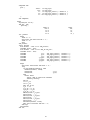
Download OCAPI User Manual v0.81

OCAPI/RT
User Manual
v0.81
(html, ps, pdf)
IMEC (Interuniversity Micro-Electronics Centre)
DESICS (Design Technology for Integrated Information and Communication Systems)
DBATE (Digital Broadband Transceivers)
Kapeldreef 75
B-3001 Leuven
Belgium
E-mail: [email protected]
1
1. Introductory Pointers
1.1. Purpose
OCAPI/RT is a C++ library intended for the design of digital systems. It provides a short
path from a system design description to implementation in hardware. The library is suited
for a variety of design tasks, including
Fixed Point Simulations
System Performance Estimation
System Profiling
Algorithm-to-Architecture Mapping
System Design according to a Dataflow Paradigm
Verification and Testbench Development
This manual is not a tutorial to digital design. Also, it is not a C++ course. It is rather a
guideline to the use of the library during system design.
The manual is set up in a bottom fashion, starting with simple concepts and constructs, and
working towards more complex ones. Starting users therefore can read the manual
front-to-back. A few tutorial examples are included as well throughout the sections.
1.2. Publication pointers
Below, some publication references are included. They can help to grasp ’the overall
picture’ behind OCAPI/RT.
Classics in the dataflow area (which is the entry specification level of OCAPI/RT) are:
"Static Scheduling of Synchronous Data Flow Graphs for Digital Signal Processing", E.
Lee et al, IEEE Trans. Computers, september 1987
"Recurrences, Iteration, and Conditionals in Statically Scheduled Block Diagram
Languages", E. Lee, VLSI Sig. Proc III
"Cyclo-Static Dataflow", G. Bilsen, M. Engels, R. Lauwereins, J. Peperstraete, IEEE
Trans. On Sig. Proc., february 1996
Related to OCAPI itself you may consult:
"Synthesis of Variable and Multiple Rate Circuits for Telecommunications
Applications", P. Schaumont, S. Vernalde, M. Engels, I. Bolsens, EDTC97
"The OCAPI Design System", IMEC
The synthesis backend of OCAPI/RT is partly based on the Cathedral-3 work:
"Accelerator Data-Path Synthesis for High-Throughput Signal Processing
Applications", W. Geurts, F. Catthoor, S. Vernalde, H. De Man, Kluwer Academic
Publishers
"Synthesis of high throughput DSP ASIC Application Specific Data Paths", S.
Vernalde, P. Schaumont, DSP & Multimedia Technology, June 1994
2
Finally, introductions to the art of digital design may be found in
"Digital Systems, Hardware, and Firmware Algorithms", M. Ercegovac, T. Lang,
Wiley
"Digital Systems: with algorithm implementation", M. Davio, A. Thayse, J.P.
Deschamps
1.3. In case of trouble
The OCAPI/RT complaint counter is at [email protected]. Do not hesitate to report any
suspicious behavior you encounter. Even if no bug is at play, you could have discovered at
least a weak point of this manual.
3
2. Development flow
2.1. The flow layout
The design flow shown in figure starts off with an untimed, floating point C++ system
description. Since data-processing intensive applications such as all-digital transceivers are
targeted, this description uses data-flow semantics. The system is described as a network of
communicating components.
At first, the design is refined, and in each component, features expressing hardware
implementation are introduced, including time (clock cycles) and bittrue rounding effects.
The use of C++ allows to express this in an elegant way. Also, all refinement is done in a
single environment, which greatly speedups the design effort.
Next, the C++ description is translated into an equivalent HDL description by code
generation. For each component, a controller description and a datapath description is
generated. This is done because we rely on separate synthesis tools for both parts, each one
optimized towards controller or else datapath synthesis tasks. Through the use of an
appropriate object modeling hierarchy the generation of datapath and controller HDL can be
done fully automatic.
For datapath synthesis, we rely on the Cathedral-3 datapath synthesis tools, that allow to
obtain a bitparallel hardware implementation starting from a set of signal flowgraphs.
Controller synthesis on the other hand is done by the logic synthesis of Synopsys DC. This
divide and conquer strategy towards synthesis allows each tool to be applied at the right
place.
During system simulation, the system stimuli are also translated into testbenches that allow
to verify the synthesis result of each component. After interconnecting all synthesized
components into the system netlist, the final implementation can also be verified using a
generated system testbench.
2.2. The system model
The system machine model that is used is a set of concurrent processes. Each process
translates to one component in the final system implementation.
At the system level, processes execute using data flow simulation semantics. That is, a
process is described as an iterative behavior, where inputs are read in at the start of an
iteration, and outputs are produced at the end. Process execution can start as soon as the
required input values are available.
Inside of each process, two types of description are possible. The first one is an untimed
description, and can be expressed using any C++ constructs available. A firing rule is also
added to allow dataflow simulation. Untimed processes are not subject to hardware
implementation but are needed to express the overal system behavior. A typical example is a
channel model used to simulate a digital transeiver.
The second flavor of processes is timed. These processes operate synchronously to the
system clock. One iteration of such a process corresponds to one clock cycle of processing.
Such a process falls apart in two pieces: a control description and a data processing
description.
4
The control description is done by means of a finite state machine, while the data description
is a set of instructions. Each instruction consists of a series of signal assignments, and can
also define process in- and outputs. Upon execution, the control description is evaluated to
select one or more instructions for execution. Next, the selected instructions are executed.
Each instruction thus corresponds to one clock cycle of RT behavior.
For system simulation, two schedulers are available. A dataflow scheduler is used to
simulate a system that contains only untimed blocks. This scheduler repeatedly checks
process firing rules, selecting processes for execution as their inputs are available. When the
system also contains timed blocks however, a cycle scheduler is used. The cycle scheduler
manages to interleave execution of multi-cycle descriptions, but can incorporate untimed
blocks as well.
5
3. The standard program
GNU is one of OCAPI/RT’s favorites. In consequence, the library is developed with the g++ C++
GNU compiler. The current version uses the g++ 2.8.1 compiler, and has been successfully
compiled and run under the following operating system platforms: HPUX-9 (HPRISC),
HPUX-10 (HPUX10), SunOS (SUN4), Solaris (SUN5) and Linux 2.0.0 (LINUX).
In this section the layout of your ’standard’ g++ OCAPI/RT program will be explained, including
compilation and linking of this program.
First of all, you should make g++ your standard compilation environment. On Linux, this is
already the case after installation. Other operating system vendors however usually have their
own proprietary C++ compiler, in order to sell you YAL (yet another license). In such cases,
install the g++ compiler on the operating system, and adapt your PATH variable such that the
shell can access the compiler. The OCAPI/RT library comes as a set of include files and a binary
lib. The include files are located under the directory called include and the binary lib under the
directory called lib.
The ’standard program’ is the minimal contents of an OCAPI/RT program. It has the following
layout.
include "qlib.h"
int main()
{
// your program goes here
}
Pretty simple indeed. The include qlib.h includes everything you need to access all classes within
OCAPI/RT.
If this program is called standard.cxx, then the following makefile will transform the source code
into an executable for you. The HOSTTYPE macro defined in the makefile changes with the
computing platform. The release of the library resides at /home/user/ocapi. You must assign
OCAPI in the makefile to this value.
OCAPI
HOSTTYPE
= /home/user/ocapi
= hppa1.1-hp-hpux10.20
LIB
INCLUDE
CC
QFLAGS
LIBS
=
=
=
=
=
$(OCAPI)/lib
$(OCAPI)/include
g++
-c -g -Wall -I${INCLUDE}
-lm
%.o: %.cxx
$(CC) $(QFLAGS) $< -o $@
TARGET = standard
all: $(TARGET)
define lnkqlib
$(CC) $^ -o $@ $(LIBS)
endef
OBJS = standard.o
6
standard: ${OBJS} $(BASE)/lib_$(HOSTTYPE)_ocapi.a
${lnkqlib}
clean:
rm -f *.o
$(TARGET)
This is a makefile for GNU’s make; other make programs can have a slightly different syntax,
especially for the definition of the lnkqlib macro. It is not the shortest possible solution for a
makefile, but it is one that works on different platforms without making assumptions about
standard compilation rules.
The compilation flags (QFLAGS) mean the following: -c selects compilation-only, -g turns on
debugging information, and -Wall will curse you to hell for confusing a reference with a pointer
(the warning flag, indeed). The debugging flag allows you to debug your program with gdb, the
GNU debugger.
Even if you don’t like a debugger and prefer the good old printf() debugging, gdb can at least be
of great help in the case your program core dumps. Start your program under gdb (type gdb
standard at the shell prompt), type run to let standard crash again, and then type bt. You now
see the call trace. There are a load of other reasons to use gdb of course.
7
4. Calculations
OCAPI/RT processes both floating point and fixed point values. In contrast to the standard C++
data types like int and double, a hybrid data type class is used, that simulates both fixed point and
floating point behavior.
4.1. The dfix class
This class is called dfix. The particular floating/fixed point behavior is selected by the class
constructor. The standard format of this constructor is
dfix a;
dfix a(0.5);
dfix a(0.5, 10, 8);
//
//
//
//
a floating point value
a floating point value with initial value
a fixed point value with initial value,
10 bits total wordlength, 8 fractional bits
A fixed point value has a maximal precision of the mantissa precision of a C++ double. On
most machines, this is 53 bits.
A fixed point value can also select a representation, an overflow behavior, and a rounding
behavior. These flags are, in this order, optional parameters to the dfix constructor. They can
have the following values.
Representation flag: dfix::tc for two’s complement signed representation, dfix::ns for
unsigned representation.
Overflow flag: dfix::wp for wrap-around overflow, dfix::st for saturation.
Rounding flag: dfix::fl for truncation (floor), dfix::rd for rounding behavior.
Some examples are
dfix a(0.5, 10, 8);
// the default is two’s complement, wrap-around,
// truncated quantisation
dfix a(0.5, 10, 8, dfix::tc, dfix::st, dfix::rd);
// two’s complement, saturation, rounding
// quantisation
dfix a(0.5, 10, 8, dfix::ns);
// unsigned, wrap-around, truncated quantisation
When working with fixed point dfixes, it is important to keep the following rule in mind:
quantisation occurs only when a value is defined or assigned. This means that a large
expression with several intermediate results will never have these intermediate values
quantised. Especially when writing code for hardware implementation, this should be kept in
mind. Also intermediate results are stored in finite hardware and therefore will have some
quantisation behavior. There is however a a cast operator that will come at help here.
4.2. The dfix operators
The operators on dfix are shown below
+, -, *, /
Standard addition, subtraction (including unary minus), multiplication and division.
+=, -=, *=, /=
In-place versions of previous operators.
abs
8
Absolute value.
<<, >>
Left and right shifts.
<<=, >>=
In-place left and right shifts.
msbpos
Most-significant bit position.
&, |, ^, ~
Bitwise and, or, exor, and not operators.
frac() (member call)
Fractional part
==, !=, <=, >=, <, >
Relational operators: equal, different, smaller then or equal to, greater then or equal to,
smaller then, greater then. These return an int instead of a dfix.
All operators with exception of the bitwise operators work on the maximal fixed point
precision (53 points). The bitwise operators have a precision of 32 bits (a C++ long). Also,
they assume the fixed point representation contains no fractional bits. This is an anomaly of
the fixed point library. The dfix type really is a mapping from a high-level type (floating
point) in a low-level type (fixed point). A good implementation of the bitwise operators
would require the presence of a high-level int, which is not present in the fixed point library.
This high-level type rather is faked with a low-level fixed point type with zero bits fractional
precision. In addition to the arithmetic operators, several utility methods are available for the
dfix class.
dfix a, b;
// cast a to another type
b = cast(dfix(0, 12, 10), a);
// assign b to a, retaining the quantisation of a
a = b;
// assign b to a, including the quantisation
a.duplicate(b);
// return the integer part of b
int c = (int) b;
// retrieve the value of b as a double
double d,e:
d = b.Val();
e = Val(b);
// return quantisation characteristics of a
a.TypeW();
// returns the number of bits
a.TypeL();
// returns the number of fractional bits
a.TypeSign();
// returns dfix::tc or dfix::ns
a.TypeOverflow(); // returns dfix::wp or dfix::st
a.TypeRound();
// returns dfix::fl or dfix::rd
// check if two dfixes are identical in value and quantisation
identical(a,b);
// see wether a is floating or fixed point
a.isDouble();
a.isFix();
// write a to cout
9
cout << a;
// write a to stdout, in float format,
// on a field of 10 characters
write(cout, a, ’f’, 10);
// now use a fixed-format
write(cout, a, ’g’, 10);
// next assume a is a fixed point number,
// and write out an integer representation
// (considering the decimal point at the lsb of a)
// use a hexadecimal format
write(cout, a, ’x’, 10);
// use a binary format
write(cout, a, ’b’, 10);
// use a decimal format
write(cout, a, ’d’, 10);
// read a from stdin
cin >> a;
10
5. Communication
Apart from values, OCAPI/RT is concerned with the communication of values in between blocks
of behavior. The high level method of communication in OCAPI/RT is a FIFO queue, of type
dfbfix. This queue is conceptually infinite in length. In practice it is bounded by a sysop
phonecall telling that you have wasted up all the swap space of the system.
5.1. The dfbfix class
A queue is declared as
dfbfix
a("a");
This creates a queue with name a. The queue is intented to pass value objects of the type
dfix. There is also an alias type of dfbfix, known as FB (flow buffer). So you can also write
FB
a("a");
2. The dfbfix operators
The basic operations on a queue allow to store and retrieve dfix objects. The operations are
dfix
dfix
dfbfix
k;
j(0.5);
a("a");
// insert j at the front of a
a.put(j);
// operator format for an insert
a << j;
// insert j at position 5, with position 0 corresponding to
// the front of a.
a.putIndex(j,5);
// read one element from the back of a
k = a.get();
// operator format for a read
a >> j;
// peek one element at position 1 of a
k = a.getIndex(1);
// operator format for peek
k = a[1];
// retrieve one element from a and throw it
a.pop();
// return the number of elements in a as an int
int n = a.getSize();
// return the name of the queue
char *p = a.name();
11
Whenever you perform an access operation that reads past the end of a FIFO, a runtime
error results, showing
Queue Underflow @ get in queue a
5.3. Utility calls for dfbfix
Besides the basic operations on queues, there are some additional utiliy operations that
modify a queue behavior
// make a queue of length 20. The default length of a queue is 16.
// whenever this length is exceeded by a put, the storage in the queue
// is dynamically expanded by a factor of 2.
dfbfix
a("a", 20);
// After the asType() call, the queue will have an input "quantizer"
// that will quantize each element inserted into the queue to that of
// the quantizer type
dfix
q(0, 10, 8);
a.asType(q);
// After an asDebug() call, the queue is associated with a file, that
// will collect every value written into the queue. The file is opened
// as the queue is initialized and closed when the queue object is destroyed.
a.asDebug("thisfile.dat");
// Next makes a duplicate queue of a, called b. Every write into a will also
// be done on b. Each queue is allowed to have at most ONE duplicate queue.
dfbfix
b("b");
a.asDup(b);
// Thus, when another duplicate is needed, you write is as
dfbfix
c("c");
b.asDup(c);
During the communication of dfix objects, the queues keep track of some statistics on the
values that are passed through it. You can use the << operator and the member function
stattitle() to make these statistics visible.
The next program demonstrates these statistics
#include "qlib.h"
void main()
{
dfbfix a("a");
a << dfix(2);
a << dfix(1);
a << dfix(3);
a.stattitle(cout);
cout << a;
}
When running this program, the following appears on screen
Name
a
put
3
get
0
MinVal @idx
1.0000e+00
2
MaxVal @idx Max# @idx
3.0000e+00
3
3
3
The first line is printed by the stattitle() call as a mnemonic for the fields printed below. The
next line is the result of passing the queue to the standard output stream object. The fields
mean the following:
12
Name
The name of the queue
put
The total number of elements put() into the queue
get
The total number of elements get() from the queue
MinVal
The lowest element put onto the queue
@idx
The put sequential number that passed this lowest element
MaxVal
The highest element put onto the queue
@idx
The put sequential number that passed this highest element
Max#
The maximal queue length that occurred
@idx
The put sequential number that resulted ion this maximal queue length
5.4. Globals derivatives for dfbfix
There are two special derivates of dfbfix. Both are derived classes such that you can use
them wherever you would use a dfbfix. Only the first will be discussed here, the other one is
related to cycle-true simulation and is discussed in Chapter 16: Faster communications.
The dfbfix_nil object is like a /dev/null drain. Every dfix written into this queue is thrown.
A read operation from such a queue results in a runtime error.
There are two global variables related to queues. The listOfFB is a pointer to a list of
queues, containing every queue object you have declared in your program. The member
function call nextFB() will return the successor of the queue in the global list. For example,
the code snippet
dfbfix *r;
for (r = listOfFB; r; r = r->nextFB())
{
...
}
will walk trough all the queues present in your OCAPI/RT program.
The other global variable is nilFB, which is of the type dfbfix_nil. It is intended to be used
as a global trashcan.
13
6. The basic block
OCAPI/RT supports the dataflow simulation paradigm. In order to define the actors to the
system, one base class is used, from which all actors will inherit. In order to do untimed
simulations, you must follow a standard template to which new actor classes must conform. In
this section, the standard template will be introduced, and the writing style is documented.
6.1. Basic block include and code file
Each new actor in the system is defined with one header file and one source code C++ file.
We define a standard block, add, which performs an addition.
The include file, add.h, looks like
#ifndef ADD_H
#define ADD_H
#include "qlib.h"
class add : public base
{
public:
//----- constructor ----add (char *name,
FB & _in1,
FB & _in2,
FB & _o1
);
//----- untimed simulation ----int run();
private :
FB
*in1;
FB
*in2;
FB
*o1;
};
#endif
This defines a class add, that inherits from base. The base object is the one that OCAPI/RT
likes to work with, so you must inherit from it in order to obtain an OCAPI/RT basic block.
The private members in the block are pointers to communication queues. Optionally, the
private members should also contain state, for example the tap values in a filter. The
management of state for untimed blocks is entirely the responsibility of the user; as far as
OCAPI/RT is concerned, it does not care what you use as extra variables.
The public members include a constructor and an execution call run. The constructor must
at least contain a name, and a list of the queues that are used for communication. Optionally,
some parameters can be passed, for instance in case of parametrized blocks (filters with a
variable number of taps and the like).
The contents of the adder block will be described in add.cxx.
#include "add.h"
//----- constructor ----add::add(char *name,
FB & _in1,
14
FB & _in2,
FB & _o1
) : base(name)
{
in1 = _in1.asSource(this);
in2 = _in2.asSource(this);
o1 = _o1 .asSink (this);
}
//----- untimed simulation: run() ----int add::run()
{
// firing rule
if ( ( in1->getSize() < 1) ||
( in2->getSize() < 1) )
{
return 0;
}
o1->put(in1->get() + in2->get());
return 1;
}
The constructor passes the name of the object to the base class it inherits from. In addition,
it initializes private members with the other parameters. In this example, the communication
queue pointers are initialized. This is not done through simple pointer assignment, but
through function calls asSource and asSink. This is not obligatory, but allows OCAPI/RT to
analyze the connectity in between the basic blocks. Since a queue is intended for
point-to-point communication, it is an error to use a queue as input or ouput more then once.
The function calls asSource and asSink keep track of which blocks source/sink which
queues. They will return a runtime error in case a queue is sourced or sinked more then
once. The constructor can optionally also be used to perform initialization of other private
data (state for instance).
The run() method contains the operations to be performed when the block is invoked. The
behavior is described in an iterative way. The run function must return an integer value, 1 if
the block succeeded in performing the operation, and 0 if this has failed
This behavior consists of two parts: a firing rule and an operative part. The firing rule must
check for the availability of data on the input queues. When no sufficient data is present
(checked with the getSize() member call), it stops execution and returns 0. When sufficient
data is present, execution can start. Execution of an untimed behavior can use the different
C++ control constructs available. In this example, the contents of the two input queues is
read, the result is added and put into the ouput queue. After execution, the value 1 is
returned to signal the behavior has completed .
6.2. Predefined standard blocks: file sources and sinks
The OCAPI/RT library contains three predefined standard blocks, which is a file source src,
a file sink snk, and a ram storage block ram.
The file sources and sinks define operating system interfaces and allow you to bring file data
into an OCAPI/RT simulation, and to write out resulting data to a file. The examples below
show various declarations of these blocks. Data in these files is formatted as floating point
numbers separated by white space. For ouput, newlines are used as whitespace.
15
// define a file source block, with name a,
// that will read data from the file "in.dat"
// and put it into the queue k
dfbfix
src
k("k");
a("a", k, "in.dat");
// an alternative definition is
dfbfix
k("k");
src
a("a", k);
a.setAttr(src::FILENAME, "in.dat");
// which also gives you a complex version
dfbfix
k1("k1");
dfbfix
k2("k2");
src
a ("a", k1, k2);
a.setAttr(src::FILENAME, "in.dat");
// define a sink block b, that will put data
// from queue o into a file "out.dat".
dfbfix
o("o");
snk
b("b", o, "out.dat");
// an alternative definition is
dfbfix
o("o");
snk
b("b", o);
b.setAttr(snk::FILENAME, "out.dat");
// which gives you also a complex version
dfbfix
o1("o1");
dfbfix
o2("o2");
snk
b ("b", o1, o2);
b.setAttr(snk::FILENAME, "out.dat");
// the snk mode has also a matlab-goodie
// which will format output data into a mtrix
// A that can be read in directly by Matlab.
dfbfix
o("o");
snk
b("b", o);
b.setAttr(snk::FILENAME, "out.m");
b.setAttr(snk::MATLABMODE, 1);
6.3. Predefined standard blocks: RAM
The ram untimed block is intended to simulate single-port storage blocks at high level. By
necessity, some interconnect assumptions had to be made on this block. On the other hand, it
is supported all the way through code generation. OCAPI/RT does not generate RAM cells.
However, it will generate appropriate connections in the resulting system netlist, onto which
a RAM cell can be connected. The declaration of a ram block is as follows.
// make a ram a, with an address bus, a data input bus, a data
// ouput bus, a read command line, a write command line, with
// 64 locations
dfbfix
dfbfix
dfbfix
dfbfix
dfbfix
address
data_in
data_out
read_c
write_c
ram
a
("address");
("data_in");
("data_out");
("read_c");
("write_c");
("a",
address,
16
data_in,
data_out,
write_c,
read_c,
64);
// clear the ram
a.clear();
// fill the ram with the linear sequence
// data = k1 + address * k2;
a.fill(k1, k2);
// dump the contents of a to cout
a.show();
The execution semantics of the ram are as follows. For each read or write, an address, a read
command and a write command must be presented. If the read command equals dfix(1), a
read will be performed, and the value stored at the location presented through address will
be put on data_out. If the read command equals any other value, a dummy byte will be
presented at data_out. If no read command was presented, no data will be presented on
data_out. For writes, an identical story holds for reads on the data_in input: Whenever a
write command is presented, the data input will be consumed. When the write command
equals 1, then the data input will be stored in the location provided through address. When a
read and write command are given at the same time, then the read will be performed before
the write. The ram also includes an online "purifier" that will generate a warning message
whenever data from an unwritten location is read.
17
7. Untimed simulations
Given the descriptions of one or more untimed blocks, a simulation can be done. The description
of a simulation requires the following to be included in a standard C++ main() procedure:
The instantiation of one or more basic blocks.
The instantiation of one or more communication queues that interconnect the blocks.
The setup of stimuli. Either these can be included at runtime by means of the standard file
source blocks, or else dedicated C++ code can be written that fills up a queue with stimuli.
A schedule that drives the execution methods of the basic blocks.
A schedule, in general, is the specification of the sequence in which block firing rules must be
tested (and fired if necessary) in order to run a simulation. There has been quite some research in
determining how such a schedule can be constructed automatically from the interconnection
network and knowledge of the block behavior. Up to now, an automatic mechanism for a general
network with arbitrary blocks has not been found. Therefore, OCAPI/RT relies on the designer to
construct such a schedule.
7.1. Layout of untimed simulation
In this section, the template of the standard simulation program will be given, along with a
description of the scheduler class that will drive the simulation. A configuration with the
adder block (described in the section on basic blocks) is used as an example.
#include "qlib.h"
#include "add.h"
void main()
{
dfbfix
i1("i1");
dfbfix
i2("i2");
dfbfix
o1("o1");
src
src
add
snk
SRC1("SRC1",
SRC2("SRC2",
ADD ("ADD",
SNK1("SNK1",
i1,
i2,
i1,
o1,
"SRC1");
"SRC2");
i2, o1);
"SNK1");
schedule S1("S1");
S1.next(SRC1);
S1.next(SRC2);
S1.next(ADD );
S1.next(SNK1);
while (S1.run());
i1.stattitle(cout);
cout << i1;
cout << i2;
cout << o1;
}
The simulation above instantiates three communication buffers, that interconnect four basic
blocks. The instantiation defines at the same time the interconnection network of the
simulation. Three of the untimed blocks are standard file sources and sinks, provided with
OCAPI/RT. The add block is a user defined one.
18
After the definition of the interconnection network, a schedule must be defined. A
simulation schedule is constructed using schedule objects. In the example, one schedule
object is defined, and the four blocks are assigned to it by means of a next() member call.
The order in which next() calls are done determines the order in which firing rules will be
tested. For each execution of the schedule object S1, the run() methods of SRC1, SRC2,
ADD and SNK1 are called, in that order. The execution method of a scheduler object is
called run(). This function returns an integer, equal to one when at least on block in the
current iteration has executed (i.e. the run() of the block has returned one). When no block
has executed, it returns zero.
The while loop in the program therefore is an execution of the simulation. Let us assume
that the directory of the simulator executable contains the two required stimuli files, SRC1
and SRC2. Their contents is as follows
SRC1
--1
2
3
SRC2
---4
5
6
-- not present in the file
-- not present in the file
When compiling and running this program, the simulator responds:
***
***
***
***
INFO:
INFO:
INFO:
INFO:
Defining block SRC1
Defining block SRC2
Defining block ADD
Defining block SNK1
Name put get
MinVal @idx
i1
3
3 1.0000e+00
1
i2
3
3 4.0000e+00
1
o1
3
3 5.0000e+00
1
MaxVal @idx Max# @idx
3.0000e+00
3
1
1
6.0000e+00
3
1
1
9.0000e+00
3
1
1
and in addition has created a file SNK1, containing
SNK1 -- not present in the file
---- -- not present in the file
5.000000e+00
7.000000e+00
9.000000e+00
The INFO message appearing on standard output are a side effect of creating a basic block.
The table at the end is produced by the print statements at the end of the program.
7.2. More on schedules
If you would examine closely which blocks are fired in which iteration, (for instance with a
debugger) then you would find
iteration 1
run SRC1 => i1 contains 1.0
run SRC2 => i2 contains 4.0
run ADD => o1 contains 5.0
run SNK1 => write out o1
schedule.run() returns 1
iteration 2
run SRC1 => i1 contains 2.0
run SRC2 => i2 contains 5.0
run ADD => o1 contains 7.0
run SNK1 => write out o1
19
schedule.run() returns 1
iteration 3
run SRC1 => i1 contains 3.0
run SRC2 => i2 contains 6.0
run ADD => o1 contains 9.0
run SNK1 => write out o1
schedule.run() returns 1
iteration 4
run SRC1 => at end-of-file, fails
run SRC2 => at end-of-file, fails
run ADD => no input tokens, fails
run SNK1 => no input tokens, fails
schedule.run() returns 0 => end simulation
There are two schedule member functions, traceOn() and traceOff(), that will produce
similar information for you. If you insert
S.traceOn();
just before the while loop, then you see
*** INFO:
*** INFO:
*** INFO:
*** INFO:
S1 [ SRC1
S1 [ SRC1
S1 [ SRC1
S1 [ ]
Defining
Defining
Defining
Defining
SRC2 ADD
SRC2 ADD
SRC2 ADD
Name
i1
i2
o1
block SRC1
block SRC2
block ADD
block SNK1
SNK1 ]
SNK1 ]
SNK1 ]
put
3
3
3
get
3
3
3
MinVal @idx
1.0000e+00
1
4.0000e+00
1
5.0000e+00
1
MaxVal @idx Max# @idx
3.0000e+00
3
1
1
6.0000e+00
3
1
1
9.0000e+00
3
1
1
appearing on the screen. This trace feature is convenient during schedule debugging.
In the simulation ouput, you can also notice that the maximum number of tokens in the
queues never exceeds one. When you had entered another schedule sequence, for example
schedule S1("S1");
S1.next(ADD );
S1.next(SRC2);
S1.next(SRC1);
S1.next(SNK1);
then you would notice that the maximum number of tokens on the queues would result in
different figures. On the other hand, the resulting data file, SNK1, will contain exactly the
same results. This demonstrates one important property of dataflow simulations: any
arbitrary but consistent schedule yields the same results. A ’consistent’ schedule means that
no block will be scheduled zero or an infinite number of times. Only the required amount of
storage will change from schedule to schedule.
7.3. Profiling in untimed simulations
Untimed simulations are not targeted to circuit implementation. Rather, they have an
explorative character. Besides the queue statistics, OCAPI/RT also enables you to do precise
profiling of operations. The requirement for this feature is that
20
1. You use schedule objects to construct the simulation
2. You describe block behavior with dfix objects
Profiling is by default enabled. To view profiling results, you send the schedule object under
consideration to the standard output stream. In the main example program given above, you
can modify this as
#include "qlib.h"
#include "add.h"
void main()
{
...
schedule S1("S1");
...
cout << S1;
}
When running the simulation, you will see the following appearing on stdout:
***
***
***
***
INFO:
INFO:
INFO:
INFO:
Defining block SRC1
Defining block SRC2
Defining block ADD
Defining block SNK1
Name put get
MinVal @idx
i1
3
3 1.0000e+00
1
i2
3
3 4.0000e+00
1
o1
3
3 5.0000e+00
1
Schedule S1 ran 4 times:
SRC1
3
SRC2
3
ADD
3
+
3
SNK1
3
MaxVal @idx Max# @idx
3.0000e+00
3
1
1
6.0000e+00
3
1
1
9.0000e+00
3
1
1
For each schedule, it is reported how many times it was run. Inside each schedule, a firing
count of each block is given. Inside each block, an operation execution count is given. The
simple add block gives the rather trivial result that there were three additions done during
the simulation.
The gain in using operation profiling is to estimate the computational requirement for each
block. For instance, if you find that you need to do 23 multiplications in a block that was
fired 5 times, then you would need at least five multipliers to guarantee the block
implementation will need only one cycle to execute.
Finally, if you want to suppress operation profiling for some blocks, then you can use the
member function call noOpsCnt() for each block. For instance, writing
ADD.noOpsCnt();
suppresses operation profiling in the ADD block.
21
8. The path to implementation
The features presented in the previous sections contain everything you need to do untimed, high
level simulations. These kind of simulations are useful for initial development. For real
implementation, more detail has to be added to the descriptions.
OCAPI/RT makes few assumptions on the target architecture of your system. One is that you
target bitparallel and synchronous hardware. Synchronicity is not a basic requirement for
OCAPI/RT. The current version however constructs single-thread simulations, and also assumes
that all hardware runs at the same clock. If different clocks need to be implemented, then a
change to the clock-cycle true simulation algorithm will have to be made. Also, it is assumed that
one basic block will eventually be implemented into one processor.
One question that comes to mind is how hardware sharing between different basic blocks can be
expressed. The answer is that you will have to construct a basic block that merges the two
behaviors of two other blocks. Some designers might feel reluctant to do this. On the other hand,
if you have to write down merged behavior, you will also have to think about the control
problems that are induced from doing this merging. OCAPI/RT will not solve this problem for
you, though it will provide you with the means to express it.
Before code generation will translate your description to an HDL, you will have to take care of
the following tasks:
1. You will have to specify wordlengths. The target hardware is capable of doing bitparallel,
fixed point operations, but not of doing floating point operations. One of your design tasks is
to perform the quantisation on floating point numbers. The dfix class discussed earlier
contains the mechanisms for expressing fixed point behavior.
2. You will have to construct a clock-cycle true description. In constructing this description,
you will not have to allocate actual hardware, but rather express which operations you
expect to be performed in which clock cycle. The semantical model for describing this clock
cycle true behavior consists of a finite state machine, and a set of signal flow graphs. Each
signal flow graph expresses one cycle of implemented behavior. This style of description
splits the control operations from data operations in your program. In contrast, the untimed
description you have used before has a common representation of control and data.
OCAPI/RT does not force an ordening on these tasks. For instance, you might first develop a
clock cycle true description on floating point numbers, and afterwards tackle the quantization
issues. This eases verification of your clock-cycle true circuit to the untimed high level
simulation.
The final implementation also assumes that all communication queues will be implemented as
wiring. They will contain no storage, nor they will be subject to buffer synthesis. In a dataflow
simulation, initial buffering values can however be necessary (for instance in the presence of
feedback loops). In OCAPI/RT, such a buffer must be implemented as an additional processor
that incorporates the required storage. The resulting system dataflow will become deadlocked
because of this. The cycle scheduler however, that simulates timed descriptions, is clever enough
to look for these ’initial tokens’ inside of the descriptions.
In the next sections, the classes that allow you to express clock cycle true behavior are
introduced.
22
9. Signals and signal flowgraphs
Some initial considerations on signals are introduced first. If you are not philosophically inclined
you might want to skip a paragraph to the hands on section.
9.1. Hardware versus Software
Software programs always use memory to store variables. In contrast, hardware programs
work with signals, which might or might not be stored into a register. This feature can be
expressed in OCAPI/RT by using the _sig class. Simply speaking, a _sig is a dfix for which
you have indicated whether is needs storage or not.
In implementation, a signal with storage is mapped to a net driven by a register, while an
immediate signal is mapped to a net driven by an operator.
Besides the storage issue, a signal also departs from the concept of scope you use in a
program. For instance, in a function you can use local variables, which are destroyed (i.e. for
which the storage is reclaimed) after you have executed the function. In hardware however,
you control the signal-to-net mapping by means of the clock signal.
Therefore you have to manage the scope of signals yourself. A syntactical effect of this is
the use of a _sig class rather then just a sig class. Within the OCAPI/RT library, a _sig
actually encapsulates a sig because OCAPI needs to distinguish between C++ scope
(procedures) and hardware scope (signal flowgraphs). The signal scope is expressed by
using a signal flowgraph object, sfg. A signal flowgraph marks a boundary on hardware
behavior, and will allow subsequent synthesis tools to find out operator allocation, hardware
sharing and signal-to-net mapping for you.
9.2. The _sig class and related operations
Hardware signals can expressed in three flavors. They can be plain signals, constant signals,
or registered signals. The following example shows how these three can be defined.
// define a plain signal a, with a floating point dfix inside of it.
_sig a("a");
// define a plain signal b, with a fixed point dfix inside of it.
_sig b("b", dfix(0,10,8));
// define a registered signal c, with an initial value k
// and attached to a clock ck.
dfix k(0.5);
clk ck;
_sig c("c", ck, k);
// define a constant signal d, equal to the value k
_sig d(k);
The registered signals, and more in particular the clock object, are explained more into detail
when signal flowgraphs and finite state machines are discussed. In this section, we will
concentrate on operations that are available for signals.
23
Using signals and signal operations, you can construct expressions. The signal operations
are a subset of the operations on dfix. This is because there is a hardware operator
implementation behind each of these operations.
+, -, *
Standard addition, subtraction (including unary minus), multiplication
&, |, ^, ~
Bitwise and, or, exor, and not operators.
==,!=,<=,>=,<,>
Relational operators.
<<,>>
Left and right shifts.
s.cassign(s1,s2)
Conditional assignment with s1 or s2 depending on s.
cast(T,s)
Convert the type of s to the type expressed in dfix T.
lu(L,s)
Use s as in index into lookuptable L and retrieve.
msbpos(s)
Return the position of the msb in s.
Precision considerations are the same as for dfix. That is, precision is at most the mantissa
precision of a double (53 bits). For the bitwise operations, 32 bits are assumed (a long). cast,
lu and msbpos are not member but friend functions. In addition, msbpos expects fixed-point
signals.
_sig a("a");
_sig b("b");
_sig c("c");
// some
c = a +
c = a c = a *
simple operations
b;
b;
b;
// bitwise operations works only on fixed point signals
_sig e(dfix(0xff, 10, 0));
_sig d("d",dfix(0,10,0));
_sig f("f",dfix(0,10,0));
f = d & e;
f = d | e;
f = ~d;
f = d ^ _sig(dfix(3,10,0));
// shifting
// a dfix is automatically promoted to a constant _sig
f = d << dfix(3,8,0);
// conditional assignment
f = (d < dfix(2,10,0)).cassign(e,d);
// type conversion is done with cast
_sig g("g",dfix(0,3,0));
g = cast(dfix(0,3,0), d);
// a lookup table is an array of unsigned long
unsigned long j = {1, 2, 3, 4, 5};
24
// a lookuptable with 5 elements, 3 bits wide
lookupTable j_lookup("j_lookup", 5, dfix(0,3,0)) = j;
// find element 2
g = lu(j_lookup, dfix(2,3,0));
If you are interested in simulation only, then you should not worry too much about type
casting and the like. However, if you intend implementation, then some rules are at hand.
These rules are induced by the hardware synthesis tools. If you fail to obey them, then you
will get a runtime error during hardware synthesis.
All operators, apart from multiplication, return a signal with the same wordlength as
the input signal.
Multiplication returns a wordlength that is the sum of the input wordlengths.
Addition, subtraction, bitwise operations, comparisons and conditional assignment
require the two input operands to have the same wordlength.
Some common pitfalls that result of this restriction are the following.
Intermediate results will, by default, not expand wordlength. In contrast, operations on
dfix do not loose precision on intermediate results. For example, shifting an 8 bit signal
up 8 positions will return you the value of zero, on 8 bits. If you want too keep up the
precision, then you must first cast the operation to the desired output wordlength,
before doing the shift.
The multiplication operator increases the wordlength, which is not automatically
reduced when you assign the result to a signal of smaller with. If you want to reduce
wordlength, then you must do this by using a cast operation.
For complex expressions, these type promotion rules look a bit tedious. They are however
used because they allow you to express behavior precisely downto the bit level. For
example, the following piece of code extracts each of the bits of a three bit signal:
_sig threebits(dfix(6,3,0));
dfix bit(0,1,0);
_sig bit2("bit2"), bit1("bit1"), bit0("bit0");
bit2 = cast(bit, threebits >> dfix(2));
bit1 = cast(bit, threebits >> dfix(1));
bit0 = cast(bit, threebits);
These bit manipulations were not possible without the given type promotion rules.
For hardware implementation, the following operators are present.
Addition and subtraction are implemented on ripple-carry adder/subtractors.
Multiplication is implemented with a booth multiplier block.
Casts are hardwired.
Shifts are either hardwired in case of constant shifts, or else a barrel shifter is used in
case of variable shifts.
Comparisons are implemented with dedicated comparators (in case of constant
comparisons), or subtractions (in case of variable comparisons).
Bitwise operators are implemented by their direct gate equivalent at the bit level.
Lookup tables are implemented as PLA blocks that are mapped using two-level or
multi-level random logic.
Conditional assignment is done using multiplexers.
25
Msbit detection is done using a dedicated msbit-detector.
9.3. Globals and utility functions for signals
There are a number of global variables that directly relate to the _sig class, as well as the
embedded sig class. As an OCAPI/RT user, the sig class is presumably invisible to you.
Hackers however always like to know more ... to do more. In normal circumstances, you do
not need to use these functions.
The variables glbNumberOf_Sig and glbNumberOfSig contain the number of _sig and sig
that your program has defined. The variable glbNumberOfReg contains the number of sig
that are of the register type. This represents the word-level register count of your design.
The glbSigHashConflicts contain the number of hash conflicts that are present in the
internal signal data structure organization. If this number is more then, say 5% of
glbNumberOf_Sig, then you might consider knocking at OCAPI/RTs complaint counter.
The simulation is not bad if you exceed this bound, only it will go s-l-o-w-e-r.
The variable glbListOfSig contains a global list of signals in your system. You can go
through it by means of
sig *run;
for (run = glbListOfSig; run; run = run->nextsig())
{
...
}
For each such a sig, you can access a number of utility member functions.
isregister() returns 1 when a signal is a register.
isconstant() returns 1 when a signal is a constant value.
isterm() returns 1 when you have defined this signal yourself. These are signals which
are introduced through _sig() class constructors. OCAPI/RT however also adds signals
of its own.
getname() returns the char * name you have used to define the signal.
get_showname() returns the char * name of the signal that is used for code generation.
This is equal to the original name, but with a unique suffix appended to it.
9.4. The sfg class
In order to construct a timed (clocked) simulation, signals and signals expressions must be
assigned to a signal flowgraph. A signal flowgraph (in the context of OCAPI/RT) is a
container that collects all behavior that must be executed during one clock cycle.
The sfg behavior contains
1. A set of expressions using signals
2. A set of inputs and ouputs that relate signals to output and input queues
Thus, a signal flowgraph object connects local behavior (the signals) to the system through
communications queues. In hardware, the indication of input and output signals also results
in ports on your resulting circuit.
26
In the philosophical paragraph at the beginning of this section, a signal flowgraph was also
indicated as a marker of hardware scope. This is also demonstrated by the following
example.
_sig
_sig
_sig
a("a");
b("b");
c(dfix(2));
dfbfix
dfbfix
A("A");
B("B");
// a signal flowgraph object is created
sfg
add_two, add_three;
// from now on, every signal expression written down will be included
// in the signal flowgraph add_two
add_two.starts();
a = b + c;
// You must also give a name to add_two, for code generation
add_two << "add_two";
// also, inputs and ouputs have to be indicated.
// you use the input and ouput objects ip and op for this
add_two << ip(b, B);
add_two << op(a, A);
// next expression will be part of add_three
add_three.starts();
a = b + dfix(3);
add_three << "add_three";
add_three << ip(b,B);
add_three << op(a,A);
// you can also to semantical checks on signal flowgraphs
add_two.check();
add_three.check();
The semantical check warns you for the following specification errors:
Your signal flowgraph contains a signal which is not declared as a signal flowgraph
input and at the same time, it is not a constant or a register. In other words, your signal
flowgraph has a dangling input.
You have written down a combinatorial loop in your signal flowgraph. Each signal
must be ultimately dependent on registered signals, constants, or signal flowgraph
inputs. If any other dependency exists, you have written down a combinatorial loop for
which hardware synthesis is not possible.
9.5. Execution of a signal flowgraph
A signal flowgraph defines one clock cycle of behavior. The semantics of a signal
flowgraph execution are well defined.
1. At the start of an execution, all input signals are defined with data fetched from input
queues.
2. The signal flowgraph output signals are evaluated in a demand driven way. That is, if
they are defined by an expression that has signal operands with known values, then the
ouput signal is evaluated. Otherwise, the unknown values of the operands are
27
determined first. It is easily seen that this is a recursive process. Signals with known
values are: registered signals, constant signals, and signals that have already been
calculated in the current execution.
3. The execution ends by writing the calculated output values to the output queues.
Signal flowgraph semantics are somewhat related to untimed blocks with firing rules. A
signal flowgraph needs one token to be present on each input queue. Only, the firing rule on
a signal flowgraph is not implemented. If the token is missing, then the simulation crashes.
This is a crude way of warning you that you are about to let your hardware evaluate a
nonsense result.
The relation with untimed block firing rules will allow to do a timed simulation which
consist partly of signal flowgraph descriptions and partly of untimed basic blocks.
Chapter12: Timed simulations will treat this more into detail.
9.6. Running a signal flowgraph by hand
A signal flowgraph is only part of a timed description. The control component (an FSM) still
needs to be introduced. There can however be situations in which you would like to run a
signal flowgraph directly. For instance, in case you have no control component, or if you
have not yet developed a control description for it.
The sfg member function run() performs the execution of the signal flowgraph as described
above. An example is used to demonstrate this.
#include "qlib.h"
void main()
{
_sig
_sig
_sig
a("a");
b("b");
c(dfix(2));
dfbfix
dfbfix
A("A");
B("B");
sfg
add_two;
add_two.starts();
a = b + c;
add_two << "add_two";
add_two << ip(b, B);
add_two << op(a, A);
add_two.check();
B << dfix(1) << dfix(2);
// running silently
add_two.eval();
cout << A.get() << "\n";
// running with debug information
add_two.eval(cout);
cout << A.get() << "\n";
add_two.eval(cout);
}
28
When running this simulation, the following appears on the screen.
3.000000e+00
add_two(
b
:
a
=>
a
4.000000e+00
add_two(Queue Underflow @ get in queue B
2)
4
4
The first line shows the result in the first eval() call. When this call is given an output stream
as argument, some additional information is printed during evaluation. For each signal
flowgraph, a list of input values is printed. Intermediate signal values are printed after the :
at the beginning of the line. The output values as they are entered in the ouput queues are
printed after the =>. Finally, the last line shows what happens when eval() is called when no
inputs are available on the input queue B.
For signal flowgraphs with registered signals, you must also control the clock of these
signals. An example of an accumulator is given next.
#include "qlib.h"
void main()
{
clk
ck;
_sig
_sig
a("a", ck, dfix(0));
b("b");
dfbfix
dfbfix
A("A");
B("B");
sfg
accu;
accu.starts();
a = a + b;
accu << "accu";
accu << ip(b, B);
accu << op(a, A);
accu.check();
B << dfix(1) << dfix(2) << dfix(3);
while (B.getSize())
{
accu.eval(cout);
accu.tick(ck);
}
}
The simulation is controlled in a while loop that will consume all input values in queue B.
After each run, the clock attached to registered signal a is triggered. This is done indirectly
through the sfg member call tick(), that updates all registered signals that have been
assigned within the scope of this sfg. Running this simulation results in the following screen
ouput
29
accu(
:
=>
accu(
:
=>
accu(
:
=>
b
a
a
b
a
a
b
a
a
1)
0/
0/
2)
1/
1/
3)
3/
3/
1
1
3
3
6
6
The registered signal a has two values: a present value (shown left of /), and a next value
(shown right of /). When the clock ticks, the next value is copied to the present value. At the
end of the simulation, registered signal a will contain 6 as its present value. The ouput queue
A however will contain the 3, the ’present value’ of a during the last iteration.
Finally, if you want to include a signal flowgraph in an untimed simulation, you must make
shure that you implement a firing rule that guards the sfg evaluation.
An example that incorporates the accumulator into an untimed basic block is the following.
#include "qlib.h"
class accu : public base
{
public:
//----- constructor ----accu
(char *
name,
dfbfix & i,
dfbfix & o);
//----- simulation ----int run();
private :
dfbfix * ipq;
dfbfix * opq;
sfg
_accu;
clk
ck;
}
//----- concstructor ----accu::accu(char *
name,
dfbfix & i,
dfbfix & o
) : base(name)
{
ipq = i.asSource(this);
opq = o.asSink(this);
_sig a("a", ck, dfix(0));
_sig b("b");
_accu.starts();
a = a + b;
_accu << "accu";
_accu << ip(b, *ipq);
_accu << op(a, *opq);
_accu.check();
}
//----- simulation: run() ----int accu::run()
{
if (ipq->getSize() < 1)
{
30
return 0;
}
_accu.eval();
_accu.tick(ck);
}
In this example, the signal flowgraph _accu is included into the private members of class
_accu.
9.7. Globals and utility functions for signal flowgraphs
The global variable glbNumberOfSfg contains the number of sfg objects that you have
constructed in your present OCAPI/RT program. Given an sfg() object, you have also a
number of utility member function calls.
getname() returns the char * name of the signal flowgraph.
merge() joins two signal flowgraphs.
getisig(int n) returns a sig * that indicates which signal corresponds to input number i
of the signal flowgraph. If 0 is returned, this input does not exist.
getiqueue(int n) returns the queue (dfbfix *) assigned to input number i of the signal
flowgraph. If 0 is returned, then this input does not exist.
getosig(int n) returns a sig * that indicates which signal corresponds to output number i
of the signal flowgraph. If 0 is returned, this output does not exist.
getoqueue(int n) returns the queue (dfbfix *) assigned to output number i of the signal
flowgraph. If 0 is returned, then this output does not exist.
You should keep in mind that a signal flowgraph is a data structure. The source code that
you have written helps to build this data structure. However, a signal flowgraph is not
executed by running your source code. Rather, it is interpreted by OCAPI/RT. You can print
this data structure by means of the cg(ostream) member call.
For example, if you appended
accu.cg(cout);
to the "running-an-sfg-by-hand" example, then the following output would be produced:
sfg accu
inputs { b_2 }
outputs { a_1 }
code
{
a_1 = a_1_at1 + b_2;
};
31
10. Finite state machines
With the aid of signals and signal flowgraphs, you are able to construct clock-cycle true data
processing behavior. On top of this data processing, a control sequencing component can be
added. Such a controller allows to execute signal flowgraphs conditionally. The controller is also
the anchoring point for true timed system simulation, and for hardware code generation. A signal
flowgraph embedded in an untimed block cannot be translated to a hardware processor: you have
to describe the control component explicitly.
10.1. The ctlfsm and state classes
The controller model currently embedded in OCAPI/RT is a Mealy-type finite state
machine. This type of FSM selects the transition to the next state based on the internal state
and the previous output value.
In an OCAPI/RT description, you use a ctlfsm object to create such a controller. In addition,
you make use of state objects to model controller states. The following example shows the
use of these objects.
#include "qlib.h"
void main()
{
sfg dummy;
dummy << "dummy";
// create a finite state machine
ctlfsm f;
// give it a name
f << "theFSM";
// create 2 states for it
state rst;
state active;
// give them a name
rst
<< "rst";
active << "active";
// identify rst as the initial state of ctlfsm f
f << deflt(rst);
// identify active as a plain state of ctlfsm f
f << active;
// create an unconditional transition from rst to active
rst << allways << active;
// create an unconditional transition from active to active,
// executing the dummy sfg.
active << allways << dummy << active;
// show what’s inside f
cout << f;
}
32
There are two states in this fsm, rst and active. Both are inserted in the fsm by means of the
<< operator. In addition, the rst state is identified as the default state of the fsm, by
embedding it into the deflt object. An fsm is allowed to have one default state. When the
fsm is simulated, then the state at the start of the first clock cycle will be rst. In the hardware
implementation, a reset pin will be added to the processor that is used to initialize the fsm’s
state register with this state.
Two transitions are defined. A transition is written according to the template: starting state,
conditions, actions, target state, all of this separated by the << operator. The condition
allways is a default condition that evaluates to true. It is used to model unconditional
transitions.
The last line of the example shows a simple operation you can do with an fsm. By relating it
to the output stream, the following will appear on the screen when you compile and execute
the example.
digraph g {
rst [shape=box];
rst->active;
active->active;
}
This output represent a textual format of the state transition diagram. The format is that of
the dotty tool, which produces a graphical layout of your state transition diagram. dotty is
commercial software available from AT&T. You cannot simulate a ctlfsm object on itself.
You must do this indirectly through the sysgen object, which is introduced in Chapter12:
Timed simulations.
10.2. The cnd class
Besides the default condition allways, you can use also boolean expressions of registered
signals. The signals need to be registered because we are describing a Mealy-type fsm. You
construct conditions through the cnd object, as shown in the next example.
#include "qlib.h"
void main()
{
clk
_sig
_sig
_sig
_sig
dfbfix
dfbfix
ck;
a("a", ck, dfix(0));
b("b", ck, dfix(0));
a_input("a_input");
b_input("b_input");
A("A");
B("B");
sfg some_operation;
// some operations go here ...
sfg readcond;
readcond.starts();
a = a_input;
b = b_input;
readcond << "readcond";
readcond << ip(a_input,A);
readcond << ip(b_input,B);
readcond.check();
// create a finite state machine
33
ctlfsm f;
f << "theFSM";
state rst;
state active;
state wait;
rst
<< "rst";
active << "active";
wait
<< "wait";
f << deflt(rst);
f << active;
f << wait;
rst
active
wait
wait
<<
<<
<<
<<
allways
_cnd(a)
(_cnd(a) && _cnd(b))
(!_cnd(a) || !_cnd(b))
<<
<<
<<
<<
readcond
readcond
readcond
readcond
<<
<<
<<
<<
active;
some_operation << wait;
wait;
active;
}
The first signal flowgraph readcond takes care of reading in two values a and b that are used
in transition conditions. The sfg reads the signals a and b in through the intermediate signals
a_input and b_input. This way, a and b are explicitly assigned in the signal flowgraph, and
the semantical check readcond.check() will not complain about unassigned signals.
The fsm below it defines three states. Besides an initial state rst and an operative state
active, a wait state wait is defined, that is entered when the input signal a is high. This is
expressed by the _cnd(a) transition condition in the second fsm transition. You must use
_cnd() instead of cnd() because of the same reason that you must use _sig() instead of sig():
The underscore-type classes are empty boxes that allocate the objects that do the real work
for you. This allocation is dynamic and independent of the C++ scope.
Once the wait state is entered, it can leave it only when the signals a or b go low. This is
indicated in the transition condition of the third fsm transition. A && operator is used to
express the and condition. If the signals a and b remain high, then the wait state is not left.
The transition condition of the last transition expresses this. It uses the logical not ! and
logical or || operators to express this.
The readcond signal flowgraph is executed at all transitions. This ensures that the signals a
and b are updated every cycle. If you fail to do this, then the value of a and b will not
change, potentially creating a deadlock.
To summarize, you can use either allways or a logical expression of _cnd() objects to
express a transition condition. The signals use in the condition must be registers. This results
in a Mealy-type fsm description. A FAQ is why condition signals must be registers, and
whether they can be plain signals also. The answer is simple: no, they can’t. The fsm control
object is a stand-alone machine that must be able to ’boot’ every clock cycle. During one
execution cycle, it will first select the transition to take (based on conditions), and then
execute the signal flowgraphs that are attached to this transition. If ’immediate’ transition
conditions had to be expressed, then the signals should be read in before the fsm transition is
made, which is not possible: the execution of an sfg can only be done when a transition is
selected, in other words: when the condition signals are known. Besides this semantical
consideration, the registered-condition requirement will also prevent you from writing
combinatorial control loops at the system level.
34
10.3. Utility functions for fsm objects
A number of utility functions on the ctlfsm and state classes are available for query
purposes. This is only minimal: The objects are intended to be manipulated by the cycle
scheduler and code generators.
sfg action;
ctlfsm f;
state s1;
state s2;
f << deflt(s1);
f << s2;
s1 << allways << s2;
s2 << allways << action << s1;
// run through all the state in f
statelist *r;
for (r = f.first; r; r = r->next)
{
...
}
// print the nuymber of states in f,
// print the number of transitions in f,
// print the name of f,
// print the number of sfg’s in f
cout << f.numstates()
<< "\n";
cout << f.numtransitions() << "\n";
cout << f.getname()
<< "\n";
cout << f.numactions()
<< "\n";
// print the name of a state
cout << s1.getname() << "\n";
35
11. The basic block for timed simulations
Using signals, signal flowgraphs, finite state machines and states, you can construct a timed
description of a block. Having obtained such a description, it is convenient to merge it with the
untimed description. This way, you will have one class that allows both timed and untimed
simulation. Of course, this merging is a matter of writing style, and nothing forces you to actually
have both a timed and untimed description for a block.
The basic block example, that was introduced in section Chapter 6: The basic block, will now be
extended with a timed version. As before, both an include file and a code file will be defined. The
include file, add.h, looks like
#ifndef ADD_H
#define ADD_H
#include "qlib.h"
class add : public base
{
public:
//----- constructor ----add (char *
name,
FB &
_in1,
FB &
_in2,
FB &
_o1);
//----- untimed simulation ----int
run();
//----- timed simulation ----void define();
ctlfsm &
fsm() { return _fsm; };
private :
FB
*in1;
FB
*in2;
FB
*o1;
ctlfsm
_fsm;
sfg
_add;
state
_go;
};
#endif
The private members now also contain a control fsm object, in addition to signal flowgraph
objects and states. If you feel this is becoming too verbose, you will find help in section Chapter
17: Faster description using macros, that defines a macro set that significantly accelerates
description entry.
In the public members, two additional member functions are declared: the define() function,
which will setup the timed description data structure, and the fsm(), which returns a pointer to the
fsm controller. Through this pointer, OCAPI/RT accesses everything it needs to do simulations
and code generation.
The contents of the adder block will be described in add.cxx.
#include "add.h"
//----- constructor ----add::add(char *
name,
36
FB
FB
FB
) :
&
_in1,
&
_in2,
&
_o1
base(name)
{
in1 = _in1.asSource(this);
in2 = _in2.asSource(this);
o1
= _o1 .asSink (this);
define();
}
//----- untimed simulation: run() ----int add::run()
{
...
}
//----- timed simulation: define() ----void add::define()
{
_sig i1("i1");
_sig i2("i2");
_sig ot("ot");
_add << "add";
_add.starts();
ot = i1 + i2;
_add << ip(i1, *in1);
_add << ip(i2, *in2);
_add << op(ot, *o1);
_fsm << "fsm";
_go << "go";
_fsm << deflt(_go);
_go << allways << _add << _go;
}
If the timed description uses also registers, then a pointer to the global clock must also be
provided (OCAPI/RT generates single-clock, synchronous hardware). The easiest way is to
extend the constructor of add with an additional parameter clk &ck, that will also be passed to the
define function.
37
12. Timed simulations
By obtaining timed descriptions for you untimed basic block, you are now ready to proceed to a
timed simulation. A timed simulation differs from an untimed one in that it proceeds clock cycle
by clock cycle. Concurrent behavior between different basic blocks is simulated on a
cycle-by-cycle basis. In contrast, in an untimed simulation, this concurrency is present on an
iteration by iteration basis.
12.1. The sysgen class
The sysgen object is for timed simulations the equivalent of a scheduler object for untimed
simulations. In addition, it also takes care of code and testbench generation, which explains
the name.
The sysgen class is used at the system level. The timed add class, defined in the previous
section, is used as an example to construct a system which uses untimed file sources and
sinks, and a timed add class.
#include "qlib.h"
#include "add.h"
void main()
{
dfbfix
i1("i1");
dfbfix
i2("i2");
dfbfix
o1("o1");
src
src
add
snk
SRC1("SRC1",
SRC2("SRC2",
ADD ("ADD",
SNK1("SNK1",
i1,
i2,
i1,
o1,
"SRC1");
"SRC2");
i2, o1);
"SNK1");
sysgen S1("S1");
S1
S1
S1
S1
<<
<<
<<
<<
SRC1;
SRC2;
ADD.fsm();
SNK1;
S1.setinfo(verbose);
clk ck;
int i;
for (i=0; i<3; i++)
{
S1.run(ck);
}
}
The simulation is set up as before with queue objects and basic blocks. Next, a sysgen object
is created, with name "S1". All basic blocks in the simulation are appended to the sysgen
objects by means of the << operator. If a timed basic block is to be used, as for instance in
case of the add object, then the fsm() pointer must be presented to sysgen rather then the
basic block itself. A sysgen object knows how to run and combine both timed and untimed
objects. For the description shown above, untimed versions of the file sources and sink src
and snk will be used, while the timed version of the add object will be used.
38
Next, three clock cycles of the system are run. This is done by means of the run(ck) member
function call of sysgen. The clock object ck is, because this simulation contains no
registered signals, a dummy object. When running the simulator executable with stimuli file
contents
SRC1
--1
2
3
SRC2
---4
5
6
-- not present in the file
-- not present in the file
you see the following appearing on the screen.
*** INFO: Defining block
*** INFO: Defining block
*** INFO: Defining block
*** INFO: Defining block
fsm fsm: transition from
add#0
add#1
in
in
sig
out’
fsm fsm: transition from
add#0
add#1
in
in
sig
out’
fsm fsm: transition from
add#0
add#1
in
in
sig
out’
SRC1
SRC2
ADD
SNK1
go to go
i1
i2
ot
ot
go to go
1
4
5
5
i1
i2
ot
ot
go to go
2
5
7
7
i1
i2
ot
ot
3
6
9
9
The debugging output produced is enabled by the setinfo() call on the sysgen object. The
parameter verbose enables full debugging information. For each clock cycle, each fsm
responds which transition it takes. The fsm of the add block is called "fsm", an as is seen it
makes transitions from the single state go to the obvious destination. Each signal flowgraph
during this simulation is executed in two phases (below it is indicated why). During
simulation, the value of each signal is printed.
12.2. Selecting the simulation verbosity
The setinfo member function call of sysgen selecs the amount of debugging information that
is produced during simulation. For values are available
silent will cause no output at all. This can significantly speed up your simulation,
especially for large systems containing several hundred of signal flowgraphs.
terse will only print the transitions that fsm’s make.
verbose will print detailed information on all signal updates.
regcontents will print a list the values of registered signals that change during the
current simulation. This is by far the most interesting option if you are debugging at the
system level: when nothing happens, for instance when all your timed descriptions are
39
in some ’hold’ mode, then no ouput is produced. When there is a lot of activity, then
you will be able to track all registered signals that change.
For instance, the code fragment
sysgen S("S");
S.setinfo(regcontents);
int cycle;
for (cycle=0; cycle < 100; cycle++)
{
cout << "> Cycle " << cycle << "\n";
S.run(ck);
}
can produce an output as shown below.
> Cycle 18
coef_ram_ir_2
copy_step_flag
ext_ready_out
pc
step_flag
0
1
1
15
1
1
0
0
16
0
coef_ram_ir_2
coef_wr_adr
hold_pc
pc
pc_ctl_ir_1
1
12
0
16
1
0
13
16
17
0
step_clock
0
1
copy_step_flag
prev_step_clock
step_flag
0
0
0
1
1
1
> Cycle 19
> Cycle 20
> Cycle 21
12.3. Two phases are better
Although you will be saved from the details behind two-phase simulation, it is worthwhile
to see the motivation behind it.
When you run an sfg ’by hand’ using the run() method of an sfg, the simulation proceeds in
one phase: read inputs, calculate, produce ouput. The sysgen object, on the other hand, uses
a two-phase simulation mechanism.
The origin is the following. In the presence of feedback loops, your system data flow
simulation will need initial values on the communication queues in order to start the
simulation. However, the code generator assumes the communication queues will translate
to wiring. Therefore, there will never be storage in the implementation of a communication
queue to hold these intitial values. OCAPI/RT works around this by producing these initial
values at runtime. This gives rise to a two-phase simulation: in the first phase, initial values
are produced, while in the second phase, they are consumed again. This process repeats
every clock cycle.
The two-phase simulation mechanism is also able to detect combinatorial loops at the
system level. If there exists such a loop, then the first phase of the simulation will not
produce any initial value on the system interconnect. Consequently, in the second phase
there will be at least one signal flowgraph that will not be able to complete execution in the
40
current clock cycle. In that case, OCAPI/RT will stop the simulation. Also, you get a list of
all signal flowgraphs that have not completed the current clock cycle, in addition to the
queue statistics that are attached to these signal flowgraphs.
41
13. Hardware code generation
This is it. This is why you have suffered all this C++ code typing: OCAPI/RT allows you to
translate all timed descriptions to a synthesizable hardware description. Regarding
implementation, you get the following in return for your coding efforts:
For each timed description, you get a datapath .dsfg file, that can be entered into the
Cathedral-3 datapath synthesis environment, converted to VHDL and postprocessed by
Synopsys-dc logic synthesis.
For each timed description, you also get a controller .dsfg file, which is synthesized through
the same environment.
You also get a glue cell, that interconnects the resulting datapath and controller VHDL file.
You get a system interconnect file, that integrates all glue cells in your system. For this
system interconnect file, you optionally can specify system inputs and outputs, scan chain
interconnects, and RAM interconnects. The file is VHDL.
Finally, you also get debug information files, that summarize the behavior of and ports on
each processor.
Untimed blocks, of course, are not translated to hardware. The use of the actual synthesis
environments will not be discussed in this section. It is assumed that you know what they do
and/or that you have a manual for them.
13.1. The generate() call
The member call generate() performs the code generation for you. In the adder example,
you just have to add
S1.generate();
at the end of the main function. If you would compile this description, and run it, then you
would see things are not quite OK:
*** INFO: Generating Systen Link Cell
*** INFO: Component generation for S1
*** INFO: C++ currently defines 5 sig, 4 _sig, 1 sfg.
*** INFO: Generating FSMD fsm
*** INFO: FSMD fsm defines 1 instructions
DSFGgen: signal i1 has no wordlength spec.
DSFGgen: signal i2 has no wordlength spec.
DSFGgen: signal ot has no wordlength spec.
DSFGgen: not all signals were quantized. Aborting.
*** INFO: Auto-cleanup of sfg
Indeed, in the adder example up to now, nothing has been entered regarding wordlengths.
During code generation, OCAPI/RT does quite some consistency checking. The general
advice in case of warnings and errors is: If you see an error or warning message, investigate
it. When you synthesize code that showed a warning or error during generation, you will
likely fail in the synthesis process too.
The add description is now extended with wordlengths. 8 bit wordlengths are chosen. You
modify the add class to include the following changes.
42
void add::define()
{
dfix wl(0,8,0);
_sig i1("i1", wl);
_sig i2("i2", wl);
_sig ot("ot", wl);
...
}
After recompiling and rerunning the OCAPI/RT program, you now see:
***
***
***
***
***
***
***
INFO:
INFO:
INFO:
INFO:
INFO:
INFO:
INFO:
Generating Systen Link Cell
Component generation for S1
C++ currently defines 5 sig, 4 _sig, 1 sfg.
Generating FSMD fsm
FSMD fsm defines 1 instructions
C++ currently defines 31 sig, 21 _sig, 3 sfg.
Auto-cleanup of sfg
In the directory where you ran this, you will find the following files:
fsm_dp.dsfg,the datapath description of add
fsm_fsm.dsfg, the controller description of add
fsm.vhd, the glue cell description of add
S1.vhd, the system interconnect cell
fsm.ports, a list of the I/O ports of add.
The glue cell fsm.vhd has the following contents (only the entity declaration part is shown).
-- Cath3 Processor for FSMD design fsm
library IEEE;
use IEEE.std_logic_1164.all;
entity fsm is
port (
reset
clk
i1
i2
ot
: in
: in
: in
: in
: out
std_logic;
std_logic;
std_logic_vector ( 7 downto 0 );
std_logic_vector ( 7 downto 0 );
std_logic_vector ( 7 downto 0 )
);
end fsm;
Each processor has a reset pin, a clock pin, and a number of I/O ports, depending on the
inputs and ouputs defined in the signal flowgraphs contained in this processor. All signals
are mapped to std_logic or std_logic_vector. The reset pin is used for synchronous reset of
the embedded finite state machine. If you need to initialize registered signals in the datapath,
then you have to describe this explicitly in a signal flowgraph, and execute this upon the
first transition out of the initial state.
The fsm.ports file, indicates which ports are read in in each transition. In the example of the
add class, there is only one transition, which results in the following .ports file:
******************** SFG fsmgogo0 *******************************
Port # I/O
Port
Q
1
I
i1
i1
2
I
i2
i2
1
O
ot
o1
43
13.2. System cell refinements
The system link cell incorporates all glue cells of your current timed system description.
These glue cells are connected if they read/write from the same system queue. There are
some refinements possible on the sysgen object that will also allow you to indicate system
level inputs and ouputs, scan chains, and RAM connections.
System inputs and ouputs are indicated with the inpad() and outpad() member calls of
sysgen. In the example, this is specified as
...
sysgen S1("S1");
dfix b8(0,8,0);
S1.inpad (i1, b8);
S1.inpad (i2, b8);
S1.outpad(o1, b8);
Making these connections will make the i1, i2, o1 signals appear in the entity declaration of
the system cell S1. The entity declaration inside of the file S1.vhd thus looks like
entity S1 is
port(
reset
clk
i1
i2
o1
: in
: in
: in
: in
: out
std_logic;
std_logic;
std_logic_vector ( 7 downto 0 );
std_logic_vector ( 7 downto 0 );
std_logic_vector ( 7 downto 0 )
);
end S1;
Scan chains can be added at the system level, too. For each scan chain you must indicate
which processors it should include. Suppose you have three basic blocks (including a timed
description and registers) with names BLOCK1, BLOCK2, BLOCK3. You attach the blocks
to two scan chains using the following code.
scanchain SCAN1("scan1");
scanchain SCAN2("scan2");
SCAN1.addscan(& BLOCK1.fsm());
SCAN1.addscan(& BLOCK2.fsm());
SCAN2.addscan(& BLOCK3.fsm());
The sysgen object identifies the required scan chain connections through the fsm objects that
are assigned to it. In order to have reasonable circuit test times, you should not include more
then 300 flip-flops in each scan chain. If you have a processor that contains more then 300
flip-flops, then you should use another scan chain connection strategy.
Finally, you can generate code for the standard untimed block RAM. There are two possible
interconnection mechanisms: the first will include the untimed RAM blocks in sysgen as
internal components of the system link cell. The second will include the RAM blocks as
external components. This latter method requires you to construct a new ’system-system
link cell’, that includes the RAM entities and the system link cell in a larger structure.
However, it might be required in case you have to remap the standard RAM interface, or
introduce additional asynchronous timing logic.
44
An example of the two methods is shown next
ram RAM1("ram1", addr1, di1, do1, wr, rd, 128);
ram RAM2("ram2", addr2, di2, do2, wr, rd, 128);
// types of address and data bus
dfix addrtype(0, 7, 0);
dfix dattype (0, 4, 0);
sysgen S1("S1");
// define an external ram
S1.extern_ram(RAM1, addrtype, dattype);
// define an internal ram
S1.intern_ram(RAM2, addrtype, dattype);
13.3. Pitfalls for code generation
As allways, there are a number of pitfalls when things get complex. You should watch the
following when diving into code generation.
OCAPI/RT tries to generate nicely formatted code, that you can investigate. To help you in
this process, also the actual signal names that you have specified are regenerated in the
VHDL and DSFG code. This implies that you have to stay away from VHDL and DSFG
keywords, or else you will get an error from either Cathedral-3 or Synopsys. An exhaustive
list is not yet made. But you can be sure that if you use names like ’port’, ’in’, ’out’, ’for’
and the like, that you will run into trouble. In case of doubt, append some numerical suffix
to your signal name, like inp1.
The mapping of the fixed point library to hardware is, in the present release, minimal. First
of all, although registered signals allow you to specify an initial value, you cannot rely on
this for the hardware circuit. Registers, when powered on, take on a random state. Therefore,
make sure that you specify the initialization sequence of your datapath. A second fixed point
pitfall is that the hardware support for the different quantization schemes is lacking. It is
assumed that you finally will use truncated quantization on the lsb-side and wrap-around
quantization on the msb-side of all signals. The other quantization schemes require
additional hardware to be included. If you really need, for instance, saturated msb
quantization, then you will have to describe it in terms of the default quantization.
Finally, the current set of hardware operators in Cathedral-3 is designed for signed
representations. They work with unsigned representations also as long as you do no use
relational operations (<, > and the like). In this last case, you should implement the unsigned
operation as a signed one with one extra bit.
45
14. Verification and testbenches
Once you have obtained a gate level implementation of your circuit, it is necessary to verify the
synthesis result. OCAPI/RT helps you with this by generating testbenches and testbench stimuli
for you while you run timed simulations and do code generations.
The example of the add class introduced previously is picked up again, and testbench generation
capability is included to the OCAPI/RT description.
14.1. Generation of testbench vectors
The next example performs a three cycle simulation of the add class and generates a
testbench vectors for it.
#include "qlib.h"
#include "add.h"
void main()
{
dfbfix
i1("i1");
dfbfix
i2("i2");
dfbfix
o1("o1");
src
src
add
snk
SRC1("SRC1",
SRC2("SRC2",
ADD ("ADD",
SNK1("SNK1",
sysgen
S1("S1");
S1
S1
S1
S1
<<
<<
<<
<<
i1,
i2,
i1,
o1,
"SRC1");
"SRC2");
i2, o1);
"SNK1");
SRC1;
SRC2;
ADD.fsm();
SNK1;
ADD.fsm().tb_enable();
clk ck;
int i;
for (i=0; i<3; i++)
{
S1.run(ck);
}
ADD.fsm().tb_data();
}
Just before the timed simulation starts, you enable the generation of testbench vectors by
means of a tb_enable() member call for each fsm that requires testbench vectors.
During simulation, the values on the input and ouput ports of the add processor are
recorded. After the simulation is done, the testbenches are generated using a tb_data()
member function call.
Testbench generation leaves three data files behind:
fsm_tb.dat contains binary vectors of all inputs of the add processor. It is intended to
be read in by the VHDL simulator as stimuli.
46
fsm_tb.dat_hex contains hexadecimal vectors of all inputs and ouputs of the add
processor. It contains the output that should be produced by the VHDL simulator when
the synthesis was successful.
fsm_tb.dat_info documents the contents of the stimuli files by saying which stimuli
vector corresponds to which signal
When compiling and running this OCAPI/RT program, the following appears on screen.
***
***
***
***
***
***
***
INFO:
INFO:
INFO:
INFO:
INFO:
INFO:
INFO:
Defining block SRC1
Defining block SRC2
Defining block ADD
Defining block SNK1
Creating stimuli monitor for testbench of FSMD fsm
Generating stimuli data file for testbench fsm_tb.
Testbench fsm_tb has 3 vectors.
Afterwards, you can take a look at each of the three generated testbenches.
-- file: fsm_tb.dat
00000001 00000100
00000010 00000101
00000011 00000110
-- file: fsm_tb.dat_hex
01 04 05
02 05 07
03 06 09
-- file: fsm_tb.dat_info
Stimuli for fsm_tb contains 3 vectors for
i1_stim
i2_stim
read
read
Next columns occur only in _hex.dat file and are outputs
o1_stim
write
14.2. Generation of testbench drivers
To generate a testbench driver, simply call the tb_enable() member function of the add fsm
before you initiate code generation. You will end up with a VHDL file fsm_tb.vhd that
contains the following driver.
-- Test Bench for FSMD design fsm
library IEEE;
use IEEE.std_logic_1164.all;
use IEEE.std_logic_textio.all;
use std.textio.all;
library clock;
use clock.clock.all;
entity fsm_tb is
end fsm_tb;
architecture rtl of fsm_tb is
signal
signal
signal
signal
signal
reset
clk
i1
i2
ot
47
:
:
:
:
:
std_logic;
std_logic;
std_logic_vector ( 7 downto 0 );
std_logic_vector ( 7 downto 0 );
std_logic_vector ( 7 downto 0 );
component fsm
port (
reset
clk
i1
i2
ot
: in
: in
: in
: in
: out
std_logic;
std_logic;
std_logic_vector ( 7 downto 0 );
std_logic_vector ( 7 downto 0 );
std_logic_vector ( 7 downto 0 )
);
end component;
begin
crystal(clk, 50 ns);
fsm_dut : fsm
port map (
reset
clk
i1
i2
ot
=>
=>
=>
=>
=>
ini: process
begin
reset <= ’1’;
wait until clk’event and clk = ’1’;
reset <= ’0’;
wait;
end process;
input: process
file stimuli : text is in "fsm_tb.dat";
variable aline : line;
file stimulo : text is out "fsm_tb.sim_out";
variable oline : line;
variable
v_i1 : std_logic_vector
variable
v_i2 : std_logic_vector
variable
v_ot : std_logic_vector
variable
v_i1_hx : std_logic_vector
variable
v_i2_hx : std_logic_vector
variable
v_ot_hx : std_logic_vector
begin
wait until reset’event and reset = ’0’;
loop
if (not(endfile(stimuli))) then
readline(stimuli, aline);
read(aline,
v_i1);
read(aline,
v_i2);
else
assert false
report "End of input file reached"
severity warning;
end if;
i1 <= v_i1;
i2 <= v_i2;
wait for 50 ns;
v_ot := ot;
v_i1_hx := v_i1;
v_i2_hx := v_i2;
v_ot_hx := v_ot;
hwrite(oline, v_i1_hx);
write(oline, ’ ’);
hwrite(oline, v_i2_hx);
write(oline, ’ ’);
hwrite(oline, v_ot_hx);
write(oline, ’ ’);
writeline(stimulo, oline);
wait until clk’event and clk = ’1’;
end loop;
end process;
end rtl;
48
reset,
clk,
i1,
i2,
ot );
(
(
(
(
(
(
7
7
7
7
7
7
downto
downto
downto
downto
downto
downto
0
0
0
0
0
0
);
);
);
);
);
);
configuration tbc_rtl of fsm_tb is
for rtl
for all : fsm
use entity work.fsm(structure);
end for;
end for;
end tbc_rtl;
The testbench uses one additional library, clock, which contains the crystal component. This
component is a simple clock generator that drives a 50% duty cycle clk.
This testbench will generate a file fsm_tb.sim_out. After running the testbench in VHDL,
this file should be exactly the same as the fsm_tb.dat_hex. You can use the unix diff
command to check this. The only possible differences can occur in the first few simulation
cycles, if the VHDL simulator initializes the registers to ‘X’.
Using automatic testbench generation greatly speedups the verification process. You should
consider using it whenever you are into code generation.
49
15. Compiled code simulations
For large designs, simulation speed can become prohibitive. The restricting factor of OCAPI/RT
is that the signal flowgraph data structures are interpreted at runtime. In addition, runtime
quantization (fixed point simulation) takes up quite some CPU power.
OCAPI/RT allows you to generate a dedicated C++ simulator, that runs compiled code instead of
interpreted code. Also, additional optimizations are done on the fixed point simulation. The result
is a simulator that runs one to two orders of magnitude faster then the interpreted OCAPI/RT
simulation. This speed increase adds up to the order of magnitude that interpreted OCAPI/RT
already gains over event-driven VHDL simulation.
As an example, a 75Kgate design was found to run at 55 cycles per second (on a HP/9000). This
corresponds to 4.1 million gates per second, and motivates why C++ is the way to go for system
synthesis.
15.1. Generating a compiled code simulator
The compiled code generator is integrated into the sysgen object. There is one member
function, compiled(), that will generate this simulator for you.
#include "qlib.h"
#include "add.h"
void main()
{
dfbfix
i1("i1");
dfbfix
i2("i2");
dfbfix
o1("o1");
add
ADD("ADD", i1, i2, o1);
sysgen
S1("S1");
S1 << ADD.fsm();
S1.compiled();
}
In this simple example, a compiled code generator is made for a design containing only one
FSM. The generator allows to include several fsm blocks, in addition to untimed blocks.
When this program is compiled and run, it leaves behind a file S1_ccs.cxx, that contains the
dedicated simulator. For the OCAPI/RT user, the simulator defines one procedure,
one_cycle(), that simulates one cycle of the system.
When calling this procedure, it also produces debugging ouput similar to the
setinfo(regcontents) call for ctlfsm objects. This procedure must be linked to a main
program that will execute the simulation.
If an untimed block is present in the system, then it will be included in the dedicated
simulator. In order to declare it, you must provide a member function CCSdecl(ofstream &)
that generates the required C++ declaration. As an example, the basic RAM block declares
itself as follows:
50
-- file: ram.h
class ram : public base
{
public:
...
ram (char *
name,
FB &
_address,
FB &
_data_in,
FB &
_data_out,
FB &
_w,
FB &
_r,
int
_size);
void CCSdecl(ofstream &os);
...
private :
...
};
-- file: ram.cxx
void
{
os
os
os
os
os
os
os
os
os
}
ram::CCSdecl(ofstream &os)
<<
<<
<<
<<
<<
<<
<<
<<
<<
" #include \"ram.h\"\n";
" ram " << typeName() << "(";
"\"" << typeName() << "\", ";
address.name() << ", ";;
data_in.name() << ", ";;
data_out.name() << ", ";
w.name() << ", ";
r.name() << ", ";
size << ");\n";
This code enables the ram to reproduce the declaration by which it was originally
constructed in the interpreted OCAPI/RT program. Every untimed block that inherits from
base, and that you whish to include in the compiled code simulator must use a similar
CCSdecl function.
15.2. Compiling and running a compiled code simulator
The compiled code simulator is compiled and linked in the same way as a normal
OCAPI/RT program. You must however also provide a main function that drives this
simulator.
The following code contains an example driver for the add compiled code simulator.
#include "qlib.h"
void one_cycle();
extern FB i1;
extern FB i2;
extern FB o1;
void main()
{
i1 << dfix(1) << dfix(2) << dfix(3);
i2 << dfix(4) << dfix(5) << dfix(6);
one_cycle();
51
one_cycle();
one_cycle();
while (o1.getSize())
{
cout << o1.get() << "\n";
}
}
When run, this program will produce the same results as before. In contrast to the compiled
simulaton of your MPEG-4 image processor, you will not be able to notice any speed
increase on this small example.
52
16. Faster communications
OCAPI/RT uses queues as a means to communicate during simulation. These queues however
take up CPU power for queue management. To save this power, there is an additional queue type,
wireFB, which is used for the simulation of point-to-point wiring connections.
16.1. The dfbfix_wire class
A wireFB does not move data. In contrast, it is related to a registered driver signal. At any
time, the value read of this queue is the value defined by the registered signal. Because of
this signal requirement, a wireFB cannot be used for untimed simulations. The following
example of an accumulator shows how you can use a wireFB, or the equivalent dfbfix_wire.
#include "qlib.h"
void main()
{
clk ck;
_sig a("a",ck,dfix(0));
_sig b("b");
dfbfix_wire A("A",a);
dfbfix
B("B");
sfg accu;
accu.starts();
a = a + b;
accu << "accu";
accu << ip(b, B);
accu << op(a, A);
accu.check();
B << dfix(1) << dfix(2) << dfix(3);
while (B.getSize())
{
accu.eval(cout);
accu.tick(ck);
}
}
A wireFB is identical in use as a normal FB. Only, for each wireFB, you indicate a
registered driver signal in the constructor.
16.2. Interconnect strategies
The wireFB object is related to the interconnect strategy that you use in your system. An
interconnect strategy includes a decision on bus-switching, bus-storage, and bus-arbitration.
OCAPI/RT does not solve this problem for you: it depends on your application what the
right interconnection strategy is.
One default style of interconnection provided by OCAPI/RT is the point-to-point, register
driven bus scheme. This means that every bus carries only one signal from one processor to
another. In addition, bus storage in included in the processor that drives the bus.
53
More complex interconnect strategies, like the one used in Cathedral-2, are also possible,
but will have to be described in OCAPI explicitly. Thus, the freedom of target architecture is
not without cost. In Chapter 18: Meta Code generation, a solution to this specification
problem is presented.
54
17. Faster description using macros
Up to now, every C++ example was given without recurring to accelerated description techniques
using macros. OCAPI/RT provides however a set of macros that saves you from a lot of extra
typing.
17.1. Macros for signals, signal flowgraphs and queues
The following macros are used for signal and signal flowgraph definition.
dfix typ(0,8,4);
clk ck;
// define a signal a with name "a"
SIG(a);
// define a signal a with name "a" and fixed wordlength w
SIGW(a,typ);
// define a constant signal
SIGC(a,dfix(3));
// define a constant, casted signal to use in signal expressions
W(typ, 0.26);
// define a clocked signal
SIGCK(a,ck,typ);
// define a dynamically allocated signal flowgraph
// and make it the current one
SFG(r);
// define an input for the current sfg
IN(signal, queue);
// define an output for the current sfg
OUT(signal, queue);
// define a queue g with name "g"
Q(g);
// read in the queue g from file "p.dat"
READQ(g,"p.dat");
// write out the queue k to file "p.dat"
WRITEQ(k,"p.dat");
The accumulator example signal flowgraph that was introduced can be described using these
macros as follows.
#include "qlib.h"
void main()
{
clk ck;
SIG(a, ck, dfix(0));
SIG(b);
Q(A);
Q(B);
SFG(accu);
a = a + b;
IN(b,B);
OUT(a,A);
B << dfix(1) << dfix(2) << dfix(3);
while (B.getSize())
55
{
accu.eval(cout);
accu.tick(ck);
}
}
17.2. Macros for finite state machines
As for signals, several macros allow you to speed up entry of the fsm descriptions. These are
especially intended to clarify the description.
ctlfsm fsm;
// set the current fsm
FSM(fsm);
// dynamically create a new state
STATE(s1);
// dynamically create the default state
INITIAL(s0);
// define an unconditional transition
SFG(action);
AT(s0) ALLWAYS DO(action) GOTO(s1);
// define a conditional transition
SIGCK(a, ck, dfix(0));
AT(s0) ON(!_cnd(a)) DO(action) GOTO(s1);
The use of dynamic allocation for signal flowgraphs and states saves you specification effort
when writing down a timed description. The adder timed description, shown earlier, can be
described in a more compact way as follows
------ in add.h
#ifndef ADD_H
#define ADD_H
#include "qlib.h"
class add : public base
{
public:
//----- constructor ----add (char *
name,
FB &
_in1,
FB &
_in2,
FB &
_o1);
//----- untimed simulation ----int run();
//----- timed simulation ----void define();
ctlfsm & fsm() { return _fsm; };
private :
FB * in1;
FB * in2;
FB * o1;
ctlfsm _fsm;
};
#endif
56
----- in add.cxx
#include "add.h"
//----- constructor ----add::add(char *
name,
FB &
_in1,
FB &
_in2,
FB &
_o1
) : base(name)
{
in1 = _in1.asSource(this);
in2 = _in2.asSource(this);
o1 = _o1 .asSink (this);
define();
}
//----- untimed simulation: run() ----int add::run()
{
...
}
//----- timed simulation: define() ----void add::define()
{
SIG(i1);
SIG(i2);
SIG(ot);
SFG(_add);
ot = i1 + i2;
IN(i1, *in1);
IN(i2, *in2);
OUT(ot, *o1);
FSM(_fsm);
INITIAL(go);
AT(go) ALLWAYS DO(_add) GOTO(go);
}
17.3. Supermacros for the standard interconnect
The standard interconnect scheme allows an even greater improvement of specification
speed. These macros make assumptions on the signal naming of system and block
interconnect to save you from most of the declarations in a timed description. First the
macros are summarized, next an example is given.
// in the class declaration .h file as private members
// plain dfbfix connections
PRT(p);
// dfbfix_wire connections
REG(p);
// as the class constructor parameters
// plain dfbfix
_PRT(p);
// dfbfix_wire
_REG(p);
// as inherited class constructors (after :base(name))
57
// plain dfbfix
IS_SIG(signal_name, type);
// dfbfix_wire
IS_REG(signal_name, clock, type);
// in the class constructor body
// plain dfbfix or dfbfix_wire, input signal
IS_IP(k);
// plain dfbfix, output signal
IS_OP(k);
// dbfix_wire, output signal
IS_RG(k);
// in signal flowgraphs, reading an input (plain dfbfix or dfbfix_wire)
GET(p);
// in signal flowgraphs, writing and ouput (plain dfbfix or dfbfix_wire)
PUT(p);
As the example, we rewrite the accumulator timed description to accumulate a stream of
input signals
-- in accu.h
#ifndef ACCU_H
#define ACCU_H
#include "qlib.h"
class accu : public base
{
public:
//----- constructor ----accu (char *
name,
clk &
ck,
_PRT
(i1),
_REG
(o1));
//----- timed simulation ----define
(clk &ck);
ctlfsm & fsm() { return _fsm; };
private :
PRT (i1);
REG (o1);
ctlfsm _fsm;
};
#endif
-- in accu.cxx
#include "accu.h"
dfix typ(0,8,0);
//----- constructor ----accu::accu(char *
name,
clk &
ck,
_PRT
(i1),
_REG
(o1)
) : base(name),
IS_SIG(i1, typ),
IS_REG(o1, ck, typ)
{
IS_IP(i1);
IS_RG(o1);
define(ck);
}
58
//----- timed simulation: define() ----void accu::define(clk &ck)
{
SFG(rst);
o1 = dfix(0);
PUT(o1);
SFG(go);
o1 = o1 + i1;
GET(i1);
PUT(o1);
FSM(_fsm);
INITIAL(rst);
STATE(go);
AT(rst) ALLWAYS DO(rst) GOTO(go);
AT(go) ALLWAYS DO(go) GOTO(go);
}
The macros hide a significant amount of declarations. In addition, they do internal renaming,
such that for example a state go is distinguished from a signal flowgraph go.
59
18. Meta-code generation
OCAPI/RT internally uses meta-code generation. With this, it is meant that there are code
generators that generate new fsm, sfg and sig objects which in turn can be translated to
synthesizable code.
Meta-code generation is a powerful method to increase the abstraction level by which a
specification can be made. This way, it is also possible to make parametrized descriptions,
eventually using conditions. VHDL is not suited to express conditional structure. You really need
some generator-method like the meta-code generation of OCAPI/RT to do this. Therefore, it is
the key method of soft-chip components, which are software programs that translate themselves
to a wide range of implementations, depending on the user requirements.
The meta-code generation mechanism is also available to you as a user. To demonstrate this, a
class will be presented that generates an ASIP datapath decoder.
18.1. An ASIP datapath idiom
An ASIP datapath, when described as a timed description within OCAPI/RT, will consist of
a number of signal flowgraphs and a finite state machine. The signal flowgraphs express the
different functions to be executed by the datapath. The fsm description is a degenerated one,
that will use one transition per decoded instruction. The transition condition is expressed by
the ’instruction’ input, and selects the appropriate signal flowgraph for execution.
Because the finite state machine has a fixed, but parametrizable structure, it is subject for
meta-code generation. You can construct a decoder object, that generates the fsm for you.
This will allow compact specification of the instruction set.
First, the decoder object (which is present in OCAPI/RT) itself is presented
-- the include file
#define MAXINS 100
#include "qlib.h"
class decoder : public base
{
public:
decoder(char *_name, clk &ck, dfbfix &_insq);
void dec(int _numinstr);
ctlfsm &fsm();
void dec(int _code, sfg &);
void dec(int _code, sfg &, sfg &);
void dec(int _code, sfg &, sfg &, sfg &);
private :
char *name;
clk *ck;
dfbfix *insq;
int inswidth;
int numinstr;
int codes[MAXINS];
ctlfsm _fsm;
state active;
sfg decode;
_sigarray *ir;
cnd * deccnd(int );
void decchk(int );
};
60
-- the .cxx file
#include "decoder.h"
static int numbits(int w)
{
int bits = 0;
while (w) {
bits++;
w = w >> 1;
}
return bits;
}
int bitset(int bitnum, int n)
{
return (n & (1 << bitnum));
}
decoder::decoder(char *_name, clk &_ck, dfbfix &_insq) : base(_name)
{
name
= _name;
insq
= _insq.asSource(this);
ck
= &_ck;
numinstr = 0;
inswidth = 0;
_fsm << _name;
// active << strapp(name,"_go_");
active << "go";
_fsm << deflt(active);
}
void
{
//
//
//
if
{
decoder::dec(int n)
define a decoder that decodes n instructions
instruction numbers are 0 to n-1
create also the instruction register
(!(n>0))
cerr << "*** ERROR: decoder " << name << " must have at least one instruction\n";
exit(0);
}
inswidth = numbits(n-1);
if (n > MAXINS)
{
cerr << "*** ERROR: decoder " << name << " exceeds decoding capacity\n";
exit(0);
}
dfix bit(0,1,0,dfix::ns);
ir = new _sigarray((char *) strapp(name,"_ir"), inswidth, ck, bit);
decode.starts();
int i;
SIGW(irw, dfix(0, inswidth, 0, dfix::ns));
for (i=0; i<inswidth; i++)
{
if (i)
{
(*ir)[i] = cast(bit, irw >> _sig(dfix(i,inswidth,0,dfix::ns)));
}
else
{
(*ir)[i] = cast(bit, irw);
}
}
decode << strapp("decod", name);
decode << ip(irw, *insq);
}
void decoder::decchk(int n)
{
// check if the decoder can decode this instruction
int i;
if (!inswidth)
{
cerr << "*** ERROR: decoder "
61
<< name << " must first define an instruction width\n";
exit(0);
}
if (n > ((1 << inswidth)-1))
{
cerr << "*** ERROR: decoder "
<< name << " cannot decode code " << n << "\n";
exit(0);
}
for (i=0; i<numinstr; i++)
{
if (n == codes[i])
{
cerr << "*** ERROR: decoder "
<< name << " decodes code " << n << " twice\n";
exit(0);
}
}
codes[numinstr] = n;
numinstr++;
}
cnd *decoder::deccnd(int n)
{
// create the transition condition that corresponds to
// the instruction number n
int i;
cnd *cresult = 0;
if (bitset(0, n))
{
cresult = &_cnd((*ir)[0]);
}
else
{
cresult = &(!_cnd((*ir)[0]));
}
for (i = 1; i < inswidth; i++)
{
if (bitset(i, n))
{
cresult = &(*cresult && _cnd((*ir)[i]));
}
else
{
cresult = &(*cresult && !_cnd((*ir)[i]));
}
}
return cresult;
}
void decoder::dec(int n, sfg &s)
{
// enter an instruction that executes one sfg
decchk(n);
active << *deccnd(n) << decode << s << active;
}
void decoder::dec(int
n,
sfg & s1,
sfg & s2)
{
// enter an instruction that executes two sfgs
decchk(n);
active << *deccnd(n) << decode << s1 << s2 << active;
}
void decoder::dec(int n,
sfg &s1,
sfg &s2,
sfg &s3)
{
// enter an instruction that executes three sfgs
decchk(n);
active << *deccnd(n) << decode << s1 << s2 << s3 << active;
}
62
ctlfsm & decoder::fsm()
{
return _fsm;
}
The main principles of generation are the following. Each instruction for the ASIP decoder
is defined as a number, in addition to one to three signal flowgraphs that need to be executed
when this instruction is decoded. The decoder object keeps track of the instruction numbers
already used and warns you if you introduce a duplicate. When the instruction number is
unique, it is split up into a number of instruction bits, and a fsm transition condition is
constructed from these bits.
18.2. The ASIP datapath at work
The use of this object is quite simple. In a timed description were you want to use the
decoder instead of a plain fsm, you inherit from this decoder object rather then from the
base class. Next, instead of the fsm description, you give the instruction list and the required
signal flowgraphs to execute.
As an example, an add/subtract ASIP datapath is defined. We select addition with
instruction number 0, and subtraction with instruction number 1.The following code (that
also uses the supermacros) shows the specification. The inheritance to decoder also
establishes the connection to the instruction queue.
-- include file
#ifndef ASIP_DP_H
#define ASIP_DP_H
class asip_dp : public decoder
{
public:
asip_dp
(char *
name,
clk &
ck,
FB &
ins,
_PRT
(in1),
_PRT(in2),
_PRT(o1));
private :
PRT (in1);
PRT (in2);
PRT (o1 );
};
-- code file
#include "asip_dp.h"
dfix typ(0,8,0);
asip_dp::asip_dp(char *
name,
clk &
ck,
FB &
ins,
_PRT
(in1),
_PRT(in2),
_PRT(o1)
) : decoder(name, ck, ins),
IS_SIG(in1, typ),
IS_SIG(in2, typ),
IS_SIG(o1, typ)
{
IS_IP(in1);
63
IS_IP(in2);
IS_OP(o1);
SFG(add);
GET(in1);
GET(in2);
o1 = in1 + in2;
PUT(o1);
SFG(sub);
GET(in1);
GET(in2);
o1 = in1 - in2;
PUT(o1);
dec(2); // decode two instructions
dec(0, SFGID(add));
dec(1, SFGID(sub));
}
64
19. Summary of classes and functions
Class
dfix
Function
Purpose
dfix dfix()
floating point
dfix dfix(double v)
initialized floating point
dfix dfix(double v,int W, int L)
initialized fixed point, width W, fraction L
dfix dfix(double v, int W, int L,
int rep, int ovf, int rnd)
initialized fixed point with quantization
dfix dfix + dfix
addition
dfix dfix - dfix
subtraction
dfix dfix * dfix
multiplication
dfix dfix / dfix
division
dfix dfix += dfix
in-place addition
dfix dfix -= dfix
in-place subtraction
dfix dfix *= dfix
in-place multiplication
dfix dfix /= dfix
in-place division
dfix abs(dfix)
absolute value
dfix dfix << dfix
left shift
dfix dfix >> dfix
right shift
dfix dfix <<= dfix
in-place left shift
dfix dfix >>= dfix
in-place right shift
dfix msbpos(dfix)
Most significant bit position
dfix dfix & dfix
Bitwise and
dfix dfix | dfix
Bitwise or
dfix ^dfix
Bitwise not
dfix dfix.frac()
Fractional part
int dfix == dfix
Equality
int dfix != dfix
Different
int dfix < dfix
Smaller then
int dfix > dfix
Greater then
int dfix <= dfix
Smaller then or equal to
int dfix >= dfix
Greater then or equal to
dfix cast(dfix W, dfix v)
Cast v to type W
dfix dfix.duplicate(dfix)
Value and Type duplication
Cast to int
int (int) dfix
65
double dfix.Val()
Return the value
double Val(dfix)
Return the value
int dfix.TypeW()
Return the width
int dfix.TypeL()
Return the fractional width
int dfix.TypeSign()
Return the representation type
int dfix.TypeOverflow()
Return the overflow type
int dfix.TypeRound()
Return the rounding type
int identical(dfix, dfix)
True if same value and type
int dfix.isDouble()
True if floating point
int dfix.isFix()
True if fixed point
Class
Function
Purpose
dfix
ostream ostream << dfix
Write dfix value
istream istream >> dfix
Read dfix value
void write(ostream, dfix, ’f’, int w) Write floating point format
void write(ostream, dfix, ’g’, int w) Write fixed format
void write(ostream, dfix, ’x’, int w) Write integer hex format
void write(ostream, dfix, ’b’, int w) Write integer binary format
void write(ostream, dfix, ’d’, int w) Write integer decimal format
dfbfix
dfbfix dfbfix(char *)
Create a queue
dfbfix dfbfix(char *, int size)
Create a queue
dfbfix FB(char *)
Create a queue
void dfbfix.put(dfix)
Enter dfix at front
dfix dfbfix.get()
Read a dfix from rear
void dfbfix.putIndex(dfix, long)
Poke dfix at position
dfix dfbfix.getIndex(long)
Peek dfix from position
dfbfix dfbfix << dfix
Enter a dfix at front
dfbfix dfbfix >> dfix
Read a dfix from rear
dfix dfbixfix [long]
Peek dfix from position
void dfbfix.clear()
Empty the queue
long dfbfix.getSize()
Return the size in elements
void dfbfix.pop()
Remove rear element
void dfbfix.pop(int)
Remove n elements from rear
Return the queue name
char * dfbfix.name()
void dfbfix.asType(dfix)
Use a quantizer
void dfbfix.asDup(dfbfix)
Attach a mirror queue
void dfbfix.asDebug(char *)
Create a trace file
66
void dfbfix.stattitle(ostream)
Print queue statistics
ostream ostream << dfbfix
base
dfbfix * dfbfix.asSource(base *)
Define a queue reader
dfbfix * dfbfix.asSink(base *)
Define a queue writer
Inherit from base block
base : public base
(virtual) untimed simulaton
int run()
void CCSdecl(ostream)
(virtual) compiled code declaration
void base.noOspCnt()
Disable operation profiling
Create a scheduler
schedule schedule schedule(char *)
void schedule.next(base)
Attach an actor
Untimed simulation
int schedule.run()
ostream ocstream << schedule
Print profiling statistics
void schedule.traceOn()
Enable runtime tracing
void schedule.traceOff()
Disable runtime tracing
Class
clk
Print statistics header
Function
Purpose
Create a clock
clk clk()
lookupTable lookupTable lookupTable(char *, int, dfix) Create a lookup table
lookupTable lookupTable = unsigned long *
_sig
Define a lookup table
_sig _sig(char *)
Create a signal
_sig _sig(char *, dfix)
Create a quantized/initialized signal
_sig _sig(char *, clk, dfix)
Create a registered signal
_sig _sig(dfix)
Create a constant signal
_sig _sig + _sig
Addition
_sig _sig - _sig
Subtraction
_sig _sig * _sig
Multiplication
_sig _sig & _sig
Bitwise and
_sig _sig | _sig
Bitwise or
_sig _sig ^_sig
Bitwise exor
_sig
Bitwise not
_sig
_sig _sig == _sig
Equality
_sig _sig != _sig
Difference
_sig _sig < _sig
Smaller then
_sig _sig > _sig
Greater then
_sig _sig <= _sig
Smaller then or Equal to
_sig _sig >= _sig
Greater then or Equal to
_sig _sig << _sig
Left shift
_sig _sig >> _sig
Right shift
_sig _sig.cassign(_sig, _sig)
Conditional assignment
67
_sig cast(dfix, _sig)
Signal type conversion
_sig lu(lookupTable, _sig)
Lookup
_sig msbpos(_sig)
Most significant bit position
Return the embedded signal
sig * _sig.Rep()
sig
sig sig()
Create a dummy signal
int sig.isregister()
True if registered signal
int sig.isconstant()
True if constan signal
int sig.isconstant()
True if constan signal
char * sig.getname()
Name of the signal
char * sig.get_showname()
Code generation name
ip
ip ip(_sig, dfbfix)
Define a sfg input
op
op op(_sig, dfbfix)
Define a sfg output
sfg
Create a sfg
sfg sfg()
Start the scope of a sfg
void sfg.starts()
Class
sfg
sfg sfg << char *
Name a sfg
sfg sfg << ip
Attach a sfg input
sfg sfg << op
Attach a sfg output
void sfg.check()
Semantical check of sfg
void sfg.eval()
Execute an sfg
void sfg.eval(ostream)
Execute and debug an sfg
Function
Purpose
Update registered signals in sfg
void sfg.tick(clk)
Get the name of an sfg
char * sfg.getname()
Merge two sfg’s
sfg sfg.merge(sfg)
sig * sfg.getisig(int)
Get input signal from sfg
sig * sfg.getosig(int)
Get output signal from sfg
dfbfix * sfg.getiqueue(int)
Get input queue from sfg
dfbfix * sfg.getoqueue(int)
Get output queue from sfg
void sfg.cg(ostream)
state
state state()
Create a state
state state << char *
Name a state
state state << _cnd
Define a transition condition
state state << sfg
Define a transition action
state state << state
Define a transition target state
char * state.getname()
deflt
ctlfsm
Show sfg structure
Name of a state
Define a default state
deflt deflt(state)
Create a fsm
ctlfsm ctlfsm()
68
ctlfsm ctlfsm << char *
Name a fsm
ctlfsm ctlfsm << state
Include a state in fsm
ctlfsm ctlfsm << deflt
Include a default state in fsm
ostream ostream << ctlfsm
int ctlfsm.numstates()
Number of states
int ctlfsm.numtransitions()
Number of transitions
int ctlfsm.numactions()
Number of sfg actions
char * ctlfsm.getname()
_cnd
Dump a fsm
Name of the fsm
void ctlfsm.tb_enable()
Enable testbench vector generation
void ctlfsm.tb_data()
Generate testbench vectors
_cnd _cnd(_sig)
Define a condition
_cnd _cnd && _cnd
Logical and
_cnd _cnd || _cnd
Logical or
_cnd ! _cnd
Logical not
scanchain scanchain scanchain(char *)
Define a scanchain
void scanchain.addscan(ctlfsm *) Include a block
sysgen
sysgen sysgen(char *)
Create a cycle scheduler
sysgen sysgen << base
Include an untimed block
sysgen sysgen << ctlfsm
Include an timed block
void sysgen.setinfo(int)
Set verbosity level
void sysgen.run(clk)
Simulate one cycle
void sysgen.generate()
Hardware code generation
void sysgen.inpad(dfbfix, dfix)
Define a system input
void sysgen.outpad(dfbfix, dfix) Define a system output
void sysgen.extern_ram(ram)
Define an external ram
void sysgen.intern_ram(ram)
Define an internal ram
void sysgen.compiled()
Generate compiled code simulator
69
OCAPI User Manual v0.81
Table of Contents
OCAPI User Manual v0.81
.
.
.
.
.
.
.
Introductory Pointers .
.
.
.
.
.
.
.
.
1. Introductory Pointers .
.
.
.
.
.
.
.
1.1. Purpose .
.
.
.
.
.
.
.
.
.
1.2. Publication pointers .
.
.
.
.
.
.
1.3. In case of trouble .
.
.
.
.
.
.
.
Development flow
.
.
.
.
.
.
.
.
.
2. Development flow
.
.
.
.
.
.
.
.
2.1. The flow layout .
.
.
.
.
.
.
.
2.2. The system model .
.
.
.
.
.
.
.
The standard program
.
.
.
.
.
.
.
.
3. The standard program .
.
.
.
.
.
.
.
Calculations .
.
.
.
.
.
.
.
.
.
.
4. Calculations .
.
.
.
.
.
.
.
.
.
4.1. The dfix class .
.
.
.
.
.
.
.
.
4.2. The dfix operators .
.
.
.
.
.
.
.
Communication .
.
.
.
.
.
.
.
.
.
5. Communication .
.
.
.
.
.
.
.
.
5.1. The dfbfix class .
.
.
.
.
.
.
.
2. The dfbfix operators
.
.
.
.
.
.
.
5.3. Utility calls for dfbfix .
.
.
.
.
.
.
5.4. Globals derivatives for dfbfix .
.
.
.
.
The basic block .
.
.
.
.
.
.
.
.
.
6. The basic block .
.
.
.
.
.
.
.
.
6.1. Basic block include and code file
.
.
.
.
6.2. Predefined standard blocks: file sources and sinks .
6.3. Predefined standard blocks: RAM .
.
.
.
Untimed simulations .
.
.
.
.
.
.
.
.
7. Untimed simulations .
.
.
.
.
.
.
.
7.1. Layout of untimed simulation .
.
.
.
.
7.2. More on schedules
.
.
.
.
.
.
.
7.3. Profiling in untimed simulations
.
.
.
.
The path to implementation .
.
.
.
.
.
.
8. The path to implementation
.
.
.
.
.
.
Signals and signal flowgraphs .
.
.
.
.
.
.
9. Signals and signal flowgraphs .
.
.
.
.
.
9.1. Hardware versus Software .
.
.
.
.
.
9.2. The _sig class and related operations
.
.
.
9.3. Globals and utility functions for signals .
.
.
9.4. The sfg class .
.
.
.
.
.
.
.
.
9.5. Execution of a signal flowgraph .
.
.
.
.
9.6. Running a signal flowgraph by hand .
.
.
.
9.7. Globals and utility functions for signal flowgraphs
Finite state machines .
.
.
.
.
.
.
.
.
10. Finite state machines .
.
.
.
.
.
.
.
10.1. The ctlfsm and state classes .
.
.
.
.
10.2. The cnd class
.
.
.
.
.
.
.
.
10.3. Utility functions for fsm objects .
.
.
.
i
.
.
.
.
.
.
.
.
.
.
.
.
.
.
.
.
.
.
.
.
.
.
.
.
.
.
.
.
.
.
.
.
.
.
.
.
.
.
.
.
.
.
.
.
.
.
.
.
.
.
.
.
.
.
.
.
.
.
.
.
.
.
.
.
.
.
.
.
.
.
.
.
.
.
.
.
.
.
.
.
.
.
.
.
.
.
.
.
.
.
.
.
.
.
.
.
.
.
.
.
.
.
.
.
.
.
.
.
.
.
.
.
.
.
.
.
.
.
.
.
.
.
.
.
.
.
.
.
.
.
.
.
.
.
.
.
.
.
.
.
.
.
.
.
.
.
.
.
.
.
.
.
.
.
.
.
.
.
.
.
.
.
.
.
.
.
.
.
.
.
.
.
.
.
.
.
.
.
.
.
.
.
.
.
.
.
.
.
.
.
.
.
.
.
.
.
.
.
.
.
.
.
.
.
.
.
.
.
.
.
.
.
.
.
.
.
.
.
.
.
.
.
.
.
.
.
.
.
.
.
.
.
.
.
.
.
.
.
.
.
.
.
.
.
.
.
.
.
.
.
.
.
.
.
.
.
.
.
.
.
.
.
.
.
.
.
.
.
.
.
.
.
.
.
.
.
.
.
.
.
.
.
.
.
.
.
.
.
.
.
.
.
.
.
.
.
.
.
.
.
.
.
.
.
.
.
.
.
.
.
.
.
.
.
.
.
.
.
.
.
.
.
.
.
.
.
.
.
.
.
.
.
.
.
.
.
.
.
.
.
.
.
.
.
.
.
.
.
.
.
.
.
.
.
.
.
.
.
.
.
.
.
.
.
.
.
.
.
.
.
.
.
.
.
.
.
.
.
.
.
.
.
.
.
1
2
2
2
2
3
4
4
4
4
6
6
8
8
8
8
11
11
11
11
12
13
14
14
14
15
16
18
18
18
19
20
22
22
23
23
23
23
26
26
27
28
31
32
32
32
33
35
The basic block for timed simulations .
.
.
.
.
11. The basic block for timed simulations .
.
.
.
Timed simulations
.
.
.
.
.
.
.
.
.
12. Timed simulations .
.
.
.
.
.
.
.
12.1. The sysgen class .
.
.
.
.
.
.
.
12.2. Selecting the simulation verbosity .
.
.
.
12.3. Two phases are better
.
.
.
.
.
.
Hardware code generation
.
.
.
.
.
.
.
13. Hardware code generation
.
.
.
.
.
.
13.1. The generate() call .
.
.
.
.
.
.
13.2. System cell refinements .
.
.
.
.
.
13.3. Pitfalls for code generation
.
.
.
.
.
Verification and testbenches .
.
.
.
.
.
.
14. Verification and testbenches .
.
.
.
.
.
14.1. Generation of testbench vectors
.
.
.
.
14.2. Generation of testbench drivers
.
.
.
.
Compiled code simulations
.
.
.
.
.
.
.
15. Compiled code simulations
.
.
.
.
.
.
15.1. Generating a compiled code simulator .
.
.
15.2. Compiling and running a compiled code simulator
Faster communications .
.
.
.
.
.
.
.
16. Faster communications .
.
.
.
.
.
.
16.1. The dfbfix_wire class .
.
.
.
.
.
.
16.2. Interconnect strategies
.
.
.
.
.
.
Faster description using macros .
.
.
.
.
.
17. Faster description using macros
.
.
.
.
.
17.1. Macros for signals, signal flowgraphs and queues
17.2. Macros for finite state machines .
.
.
.
17.3. Supermacros for the standard interconnect .
.
Meta-code generation .
.
.
.
.
.
.
.
.
18. Meta-code generation
.
.
.
.
.
.
.
18.1. An ASIP datapath idiom .
.
.
.
.
.
18.2. The ASIP datapath at work
.
.
.
.
.
Summary of classes and functions .
.
.
.
.
.
19. Summary of classes and functions .
.
.
.
.
ii
.
.
.
.
.
.
.
.
.
.
.
.
.
.
.
.
.
.
.
.
.
.
.
.
.
.
.
.
.
.
.
.
.
.
.
.
.
.
.
.
.
.
.
.
.
.
.
.
.
.
.
.
.
.
.
.
.
.
.
.
.
.
.
.
.
.
.
.
.
.
.
.
.
.
.
.
.
.
.
.
.
.
.
.
.
.
.
.
.
.
.
.
.
.
.
.
.
.
.
.
.
.
.
.
.
.
.
.
.
.
.
.
.
.
.
.
.
.
.
.
.
.
.
.
.
.
.
.
.
.
.
.
.
.
.
.
.
.
.
.
.
.
.
.
.
.
.
.
.
.
.
.
.
.
.
.
.
.
.
.
.
.
.
.
.
.
.
.
.
.
.
.
.
.
.
.
.
.
.
.
.
.
.
.
.
.
.
.
.
.
.
.
.
.
.
.
.
.
.
.
.
.
.
.
.
.
.
.
.
.
.
.
.
.
.
.
.
.
.
.
.
.
.
.
.
.
.
.
.
.
.
.
.
.
.
.
.
.
.
.
.
.
.
.
.
.
.
.
.
.
.
.
.
.
.
.
.
.
.
.
.
.
.
.
.
.
.
.
.
.
.
.
.
.
.
.
.
.
.
.
36
36
38
38
38
39
40
42
42
42
44
45
46
46
46
47
50
50
50
51
53
53
53
53
55
55
55
56
57
60
60
60
63
65
65