Download VnmrJ Imaging User Guide

VnmrJ Imaging
User Guide
Varian MR Systems
With VnmrJ 2.2B Software
Pub. No. 01-999344-00, Rev. A 0207
VnmrJ Imaging
User Guide
Varian MR Systems
With VnmrJ 2.2B Software
Pub. No. 01-999344-00, Rev. A 0207
NOTICE: Varian, Inc. was acquired by Agilent
Technologies in May 2010. This document is provided
as a courtesy but is no longer kept current and thus
will contain historical references to Varian. For more
information, go to www.agilent.com/chem.
VnmrJ Imaging User Guide
Varian MR Systems
With VnmrJ 2.2B Software
Pub. No. 01-999344-00, Rev. A 0207
Revision history
A 0207 initial release for VnmrJ 2.2B
Applicability of manual:
Imaging modules on Varian NMR superconducting spectrometer systems with VnmrJ
software.
Technical contributors: Maj Hedehus, Subramaniam Sukumar Bayard Fetler, Dan
Iverson, Mamta Rani, He Liu, Simon Chu, Chris Price, Alan Rath
Technical writer and editor: Everett Schreiber
Copyright 2005— 2007 by Varian, Inc.
3120 Hansen Way, Palo Alto, California 94304
1-800-356-4437
http://www.varianinc.com
All rights reserved. Printed in the United States.
The information in this document has been carefully checked and is believed to be
entirely reliable. However, no responsibility is assumed for inaccuracies. Statements in
this document are not intended to create any warranty, expressed or implied.
Specifications and performance characteristics of the software described in this manual
may be changed at any time without notice. Varian reserves the right to make changes in
any products herein to improve reliability, function, or design. Varian does not assume
any liability arising out of the application or use of any product or circuit described
herein; neither does it convey any license under its patent rights nor the rights of others.
Inclusion in this document does not imply that any particular feature is standard on the
instrument.
Varian, Inc. NMR Spectrometer Systems, VnmrJ, VNMR, MAGICAL II, Magnex,
AutoLock, AutoShim, AutoPhase, limNET, ASM, and SMS are registered trademarks or
trademarks of Varian, Inc. Sun, Solaris, CDE, Suninstall, Ultra, SPARC, SPARCstation,
SunCD, and NFS are registered trademarks or trademarks of Sun Microsystems, Inc. and
SPARC International. Oxford is a registered trademark of Oxford Instruments LTD.
Ethernet is a registered trademark of Xerox Corporation. VxWORKS and VxWORKS
POWERED are registered trademarks of WindRiver Inc. Other product names in this
document are registered trademarks or trademarks of their respective holders.
Overview of Contents
SAFETY PRECAUTIONS .................................................................................. 13
Introduction ...................................................................................................... 17
Chapter 1. Setting Up an Imaging System .................................................... 19
Chapter 2. Running an Imaging Study .......................................................... 25
Chapter 3. Prescan .......................................................................................... 33
Chapter 4. Protocols for Imaging ................................................................... 51
Chapter 5. Image Viewing and Review Queue ............................................ 119
Chapter 6. Interactive Image Planning ........................................................ 139
Chapter 7. Image Processing in VnmrJ ....................................................... 149
Chapter 8. Math Processing ......................................................................... 169
Chapter 9. Digital Eddy Current Compensation ......................................... 191
Appendix A. VnmrJ Imaging Interface ..........................................................197
Appendix B. Locator .......................................................................................213
Appendix C. DICOM ® Conformance Statements..........................................221
Appendix D. NMR Imaging Concepts ............................................................229
Index ................................................................................................................ 249
01-999344-00 A 0207
VnmrJ Imaging User Guide for VnmrJ 2.2B
3
4
VnmrJ Imaging User Guide for VnmrJ 2.2B
01-999344-00 A 0207
Table of Contents
SAFETY PRECAUTIONS .................................................................................. 13
Introduction ...................................................................................................... 17
Chapter 1. Setting Up an Imaging System .................................................... 19
1.1
1.2
1.3
1.4
1.5
1.6
1.7
Configuring VnmrJ for Imaging .................................................................................
System Settings for Using Imaging Pulse Sequences .................................................
Setting the gcoil Parameter .........................................................................................
Setting Parameters for Imaging Pulse Sequences .......................................................
Using Single-Pulse Sequence for Initial Setup ...........................................................
Calibrating the Pulse Length .......................................................................................
Parameters Not Normally Used for Imaging ..............................................................
19
20
21
22
23
24
24
Chapter 2. Running an Imaging Study .......................................................... 25
2.1
2.2
2.3
2.4
Running a New Study .................................................................................................
Creating Protocols .......................................................................................................
Reviewing a Previous Study .......................................................................................
Continuing a Previous Study ......................................................................................
25
30
31
31
Chapter 3. Prescan .......................................................................................... 33
3.1
3.2
3.3
3.4
3.5
3.6
3.7
Automated Prescan .....................................................................................................
Prescan Functions .......................................................................................................
Manual Prescan ...........................................................................................................
Coil Table ....................................................................................................................
Other Prescan Parameters ...........................................................................................
Setting Up and Calibrating 3D Gradient Shimming ...................................................
Troubleshooting ..........................................................................................................
33
35
39
42
44
44
48
Chapter 4. Protocols for Imaging ................................................................... 51
4.1 Imaging Protocols ....................................................................................................... 51
4.2 Standard Sequence Options ...................................................................................... 114
4.3 Commands, Macros, and Parameters ........................................................................ 116
Chapter 5. Image Viewing and Review Queue ............................................ 119
5.1
5.2
5.3
5.4
5.5
5.6
5.7
Image Display and Manipulation Tools ....................................................................
Review Queue and Organizing Images .....................................................................
Image Annotation Editor ..........................................................................................
Regions of Interest ....................................................................................................
Using and Creating Accelerator Keys ......................................................................
Drag and Drop on Graphics Canvas .........................................................................
Review Queue Command (aipRQcommand) Options ..............................................
119
120
124
125
126
130
130
Chapter 6. Interactive Image Planning ........................................................ 139
6.1 Scan Types ................................................................................................................ 139
01-999344-00 A 0207
VnmrJ Imaging User Guide for VnmrJ 2.2B
5
Table of Contents
6.2
6.3
6.4
6.5
6.6
6.7
6.8
6.9
General Features .......................................................................................................
Starting Image Planning ............................................................................................
Using Marks in Image Planning ...............................................................................
Overlays ....................................................................................................................
Display Options ........................................................................................................
Copying Current Planning to a New Protocol ..........................................................
Saving and Retrieving Prescriptions .........................................................................
Commands ................................................................................................................
140
141
141
142
144
145
145
145
Chapter 7. Image Processing in VnmrJ ....................................................... 149
7.1
7.2
7.3
7.4
Image Processing Controls .......................................................................................
Image Processing ......................................................................................................
Processing Images .....................................................................................................
Advanced Image Processing Commands ..................................................................
149
159
161
166
Chapter 8. Math Processing ......................................................................... 169
8.1
8.2
8.3
8.4
8.5
8.6
Opening Image Math ................................................................................................
Image Math Expressions ...........................................................................................
Image Math Functions ..............................................................................................
The fit Program .........................................................................................................
Signal-to-Noise Ratio, Ghosting, and Related Functions .........................................
Problems with Image Math .......................................................................................
169
170
171
179
186
190
Chapter 9. Digital Eddy Current Compensation ......................................... 191
9.1 The DECC Module .................................................................................................... 191
9.2 Theory of Preemphasis ............................................................................................. 191
9.3 Using the Decctool Interface .................................................................................... 193
Appendix A. VnmrJ Imaging Interface .........................................................197
A.1 Main Menu Bar ........................................................................................................
A.2 System Tool Bar .......................................................................................................
A.3 User Toolbar ............................................................................................................
A.4 Hiding and Showing the Toolbars ............................................................................
A.5 Locator .....................................................................................................................
A.6 Study Queue .............................................................................................................
A.7 Review Queue ..........................................................................................................
A.8 Graphics Toolbars ....................................................................................................
A.9 Advanced Function Bar ...........................................................................................
A.10 Graphics Canvas ....................................................................................................
A.11 Viewports ...............................................................................................................
A.12 Folders ....................................................................................................................
A.13 Action Controls ......................................................................................................
A.14 Hardware Bar .........................................................................................................
198
202
203
203
204
204
204
205
209
210
210
211
211
211
Appendix B. Locator ......................................................................................213
B.1 Locator Settings and Interface Elements .................................................................. 214
B.2 Using the Locator ..................................................................................................... 216
B.3 Locator Statements ................................................................................................... 217
6
VnmrJ Imaging User Guide for VnmrJ 2.2B
01-999344-00 A 0207
Table of Contents
Appendix C. DICOM ® Conformance Statements .........................................221
C.1 DICOM Conformance Statements for Storage on VnmrJ ........................................ 221
C.2 DICOM Conformance Statements for Print-SCU on VnmrJ ................................... 221
C.3 Dicom File Generation ............................................................................................. 224
Appendix D. NMR Imaging Concepts ...........................................................229
D.1 Basic Imaging Principles .........................................................................................
D.2 Time Domain to Spatial Domain Conversion ..........................................................
D.3 Logical to Laboratory Axes Transformation ............................................................
D.4 Slice Selection ..........................................................................................................
D.5 Frequency Encoding ................................................................................................
D.6 Phase Encoding ........................................................................................................
D.7 Image Resolution .....................................................................................................
D.8 Spatial Frame of Reference ......................................................................................
D.9 Image Reconstruction ..............................................................................................
D.10 Important Imaging Parameters ...............................................................................
229
230
233
235
239
241
242
244
245
245
Index ................................................................................................................ 249
01-999344-00 A 0207
VnmrJ Imaging User Guide for VnmrJ 2.2B
7
Table of Contents
8
VnmrJ Imaging User Guide for VnmrJ 2.2B
01-999344-00 A 0207
List of Figures
List of Figures
Figure 1. Study Queue .................................................................................................................... 26
Figure 2. Study Panel...................................................................................................................... 26
Figure 3. Setting Up to Acquire a Scot Image................................................................................ 27
Figure 4. Prescan Adv Page............................................................................................................ 39
Figure 5. Frequency Prescan Acquire Page.................................................................................... 40
Figure 6. 3D Shimming Prescan Page ............................................................................................ 41
Figure 7. Prescan Acquire Page for Shimming .............................................................................. 41
Figure 8. Selecting a Coil on Prescan Setup Page .......................................................................... 42
Figure 9. Manual Shim Page .......................................................................................................... 45
Figure 10. Effects of Optimization of the Images Produced .......................................................... 58
Figure 11. Well-optimized Reference ............................................................................................. 58
Figure 12. Improperly Set values for tep and groa .................................................................... 59
Figure 13. ge3dshim Example Scan, Acq, and Map pages ............................................................ 73
Figure 14. Sagittal (RO-PE1) planes .............................................................................................. 73
Figure 15. Sagittal planes from the (Base) Field Map.................................................................... 74
Figure 16. Field Variation in z-Direction........................................................................................ 75
Figure 17. Sagittal Planes from z1c.f.fdf file.................................................................................. 75
Figure 18. Line profile from Figure 17, along z-Direction............................................................. 76
Figure 19. Shimmap (z2c.f.fdf) of the z2 Shim Coil ...................................................................... 76
Figure 20. Line Profile Along the Z-Direction, from Figure 19..................................................... 76
Figure 21. XZ-Shimmap, Sagittal (RO - PE) Planes...................................................................... 76
Figure 22. Line Profile From a Planes Shown in Figure 21 ........................................................... 77
Figure 23. X2Y2 Shim Map Sagittal (RO-PE1) Planes ................................................................. 77
Figure 24. X2Y2 Shim Map Transverse (RO-PE1) Planes ............................................................ 77
Figure 25. Line Profile From Figure 24.......................................................................................... 78
Figure 26. Phase Difference Image, yz.B.wf.fdf ............................................................................ 78
Figure 27. Line Profile from Figure 26 .......................................................................................... 78
Figure 28. Selecting Zerofill Option for ge3dshim ........................................................................ 80
Figure 29. Interface for ge3dshim Shimming................................................................................. 81
Figure 30. Shim Map Shim Calculations........................................................................................ 83
Figure 31. Water Suppr Parameter Page......................................................................................... 99
Figure 32. Optimizing the Delay .................................................................................................. 100
Figure 33. Image display and manipulation tools......................................................................... 119
Figure 34. Image Annotation Editor............................................................................................. 124
Figure 35. Interactive Image Planning Interface .......................................................................... 140
Figure 36. Showing Frames.......................................................................................................... 160
Figure 37. Utilities Panel .............................................................................................................. 161
Figure 38. Image Colormap Window ........................................................................................... 163
Figure 39. Point Info Panel........................................................................................................... 164
Figure 40. Line Profile Panel........................................................................................................ 164
Figure 41. Settings Panel .............................................................................................................. 166
Figure 42. maxof.c File............................................................................................................. 173
Figure 43. Fragment of shamesfit.c File............................................................................... 184
01-999344-00 A 0207
VnmrJ Imaging User Guide for VnmrJ 2.2B
9
List of Figures
Figure 44. FUNCTION Specifications.........................................................................................
Figure 45. SNR Input and Output images ....................................................................................
Figure 46. Stats: Input and Output Images ...................................................................................
Figure 47. DECC Module Block Diagram ...................................................................................
Figure 48. RF Pulse-Acquire Sequence........................................................................................
Figure 49. decctool Window.........................................................................................................
Figure 50. Generic Locator Statement..........................................................................................
Figure 51. Frequency Spectrum Produced by an NMR Signal ....................................................
Figure 52. Effect of a Field Gradient Along Direction y ..............................................................
Figure 53. Frequency Ranges .......................................................................................................
Figure 54. 2D Image Resulting from a Slice Selection ................................................................
Figure 55. Rectangular Profile......................................................................................................
Figure 56. Slice Profile.................................................................................................................
Figure 57. Sinc Function, Truncated Sinc Pulse, and Gaussian-Shaped Slice Profiles................
Figure 58. Multislice Excitation ...................................................................................................
Figure 59. Signal Loss Restoration...............................................................................................
Figure 60. Readout Gradient and Gradient Echo..........................................................................
Figure 61. Gradient Echo Imaging Sequence...............................................................................
Figure 62. Image Resolution of Three Water-Filled Spheres .......................................................
Figure 63. Horizontal Magnet.......................................................................................................
Figure 64. Vertical Magnet ...........................................................................................................
Figure 65. Signal Intensity............................................................................................................
Figure 66. Equilibrium Magnetization .........................................................................................
10
VnmrJ Imaging User Guide for VnmrJ 2.2B
01-999344-00 A 0207
184
187
188
192
193
194
218
231
231
232
236
236
237
237
238
239
240
241
243
244
245
246
247
List of Tables
Table 1. System Components for the ge3dshim Example ............................................................. 72
Table 2. Parameters for ge3dshim Example .................................................................................. 72
Table 3. Imaging Pulse Sequence Commands, Macros, and Parameters .................................... 116
Table 4. Standard Accelerator Keys ............................................................................................ 127
Table 5. Examples of Accelerator Keys and Commands ............................................................ 127
Table 6. Scan Types ..................................................................................................................... 139
Table 7. Image Planning Prescription Menu Options .................................................................. 141
Table 8. Display Options ............................................................................................................. 144
Table 9. Planning Status Codes .................................................................................................... 145
Table 10. Image Planning Functions ........................................................................................... 146
Table 11. Image Planning Parameters .......................................................................................... 148
Table 12. Key Combinations ....................................................................................................... 160
Table 13. Image Processing Commands ...................................................................................... 166
Table 14. Fit Types ....................................................................................................................... 180
Table 15. Standard Orientations ................................................................................................... 233
Table 16. Experimental Macros and Parameters ......................................................................... 239
Table 17. Relaxation Times ......................................................................................................... 246
01-999344-00 A 0207
VnmrJ Imaging User Guide for VnmrJ 2.2B
11
List of Tables
12
VnmrJ Imaging User Guide for VnmrJ 2.2B
01-999344-00 A 0207
SAFETY PRECAUTIONS
SAFETY PRECAUTIONS
The following warning and caution notices illustrate the style used in Varian manuals for
safety precaution notices and explain when each type is used:
This symbol might be used on warning labels attached to the equipment. When
you see this symbol, refer to the relevant manual for the information referred to
by the warning label.
WARNING: Warnings are used when failure to observe instructions or precautions
could result in injury or death to humans or animals, or significant
property damage.
CAUTION: Cautions are used when failure to observe instructions could result in
serious damage to equipment or loss of data.
Warning Notices
Observe the following precautions during installation, operation, maintenance, and repair
of the instrument. Failure to comply with these warnings, or with specific warnings
elsewhere in Varian manuals, violates safety standards of design, manufacture, and
intended use of the instrument. Varian assumes no liability for customer failure to comply
with these precautions.
WARNING: Persons with implanted or attached medical devices such as
pacemakers and prosthetic parts must remain outside the 5-gauss
perimeter from the centerline of the magnet.
The superconducting magnet system generates strong magnetic fields that can
affect operation of some cardiac pacemakers or harm implanted or attached
devices such as prosthetic parts and metal blood vessel clips and clamps.
Pacemaker wearers should consult the user manual provided by the pacemaker
manufacturer or contact the pacemaker manufacturer to determine the effect on
a specific pacemaker. Pacemaker wearers should also always notify their
physician and discuss the health risks of being in proximity to magnetic fields.
Wearers of metal prosthetics and implants should contact their physician to
determine if a danger exists.
Refer to the manuals supplied with the magnet for the size of a typical 5-gauss
stray field. This gauss level should be checked after the magnet is installed.
WARNING: Keep metal objects outside the 10-gauss perimeter from the centerline
of the magnet.
The strong magnetic field surrounding the magnet attracts objects containing
steel, iron, or other ferromagnetic materials, which includes most ordinary
tools, electronic equipment, compressed gas cylinders, steel chairs, and steel
carts. Unless restrained, such objects can suddenly fly towards the magnet,
causing possible personal injury and extensive damage to the probe, dewar, and
superconducting solenoid. The greater the mass of the object, the more the
magnet attracts the object.
Only non ferromagnetic materials—plastics, aluminum, wood, nonmagnetic
stainless steel, etc.—should be used in the area around the magnet. If an object
01-999344-00 A 0207
VnmrJ Imaging User Guide for VnmrJ 2.2B
13
SAFETY PRECAUTIONS
is stuck to the magnet surface and cannot easily be removed by hand, contact
Varian service for assistance.
Refer to the manuals supplied with the magnet for the size of a typical 10-gauss
stray field. This gauss level should be checked after the magnet is installed.
WARNING: Only qualified maintenance personnel shall remove equipment covers
or make internal adjustments.
Dangerous high voltages that can kill or injure exist inside the instrument.
Before working inside a cabinet, turn off the main system power switch located
on the back of the console.
WARNING: Do not substitute parts or modify the instrument.
Any unauthorized modification could injure personnel or damage equipment
and potentially terminate the warranty agreements and/or service contract.
Written authorization approved by a Varian, Inc. product manager is required
to implement any changes to the hardware of a Varian NMR spectrometer.
Maintain safety features by referring system service to a Varian service office.
WARNING: Do not operate in the presence of flammable gases or fumes.
Operation with flammable gases or fumes present creates the risk of injury or
death from toxic fumes, explosion, or fire.
WARNING: Leave area immediately in the event of a magnet quench.
If the magnet should quench (sudden appearance of gasses from the top of the
dewar), leave the area immediately. Sudden release of helium or nitrogen gases
can rapidly displace oxygen in an enclosed space creating a possibility of
asphyxiation. Helium will displace air from the top of a room and cold nitrogen
can displace air from the lower levels of a room. Do not return until the oxygen
level returns to normal.
WARNING: Avoid helium or nitrogen contact with any part of the body.
Cold gasses or liquids (helium and nitrogen) contacting the body can cause an
injury similar to a burn. Never place your head over the helium and nitrogen
exit tubes on top of the magnet. If cold gasses or liquids contact the body, seek
immediate medical attention, especially if the skin is blistered or the eyes are
affected.
WARNING: Do not look down the upper barrel.
Unless the probe is removed from the magnet, never look down the upper
barrel. You could be injured by the sample tube as it ejects pneumatically from
the probe.
WARNING: Do not exceed the boiling or freezing point of a sample during variable
temperature experiments.
A sample tube subjected to a change in temperature can build up excessive
pressure, which can break the sample tube glass and cause injury by flying glass
14
VnmrJ Imaging User Guide for VnmrJ 2.2B
01-999344-00 A 0207
SAFETY PRECAUTIONS
and toxic materials. To avoid this hazard, establish the freezing and boiling
point of a sample before doing a variable temperature experiment.
WARNING: Support the magnet and prevent it from tipping over.
The magnet dewar has a high center of gravity and could tip over in an
earthquake or after being struck by a large object, injuring personnel and
causing sudden, dangerous release of nitrogen and helium gasses from the
dewar. Therefore, the magnet must be supported by at least one of two methods:
with ropes suspended from the ceiling or with the antivibration legs bolted to
the floor. Refer to the Installation Planning Manual for details.
WARNING: Do not remove the relief valves on the vent tubes.
The relief valves prevent air from entering the nitrogen and helium vent tubes.
Air that enters the magnet contains moisture that can freeze, causing blockage
of the vent tubes and possibly extensive damage to the magnet. It could also
cause a sudden dangerous release of nitrogen and helium gases from the dewar.
Except when transferring nitrogen or helium, be certain that the relief valves are
secured on the vent tubes.
WARNING: On magnets with removable quench tubes, keep the tubes in place
except during helium servicing.
On Varian 200- and 300-MHz 54-mm magnets only, the dewar includes
removable helium vent tubes. If the magnet dewar should quench (sudden
appearance of gases from the top of the dewar) and the vent tubes are not in
place, the helium gas would be partially vented sideways, possibly injuring the
skin and eyes of personnel beside the magnet. During helium servicing, when
the tubes must be removed, follow carefully the instructions and safety
precautions given in the manual supplied with the magnet.
Caution Notices
Observe the following precautions during installation, operation, maintenance, and repair
of the instrument. Failure to comply with these cautions, or with specific cautions
elsewhere in Varian manuals, violates safety standards of design, manufacture, and
intended use of the instrument. Varian assumes no liability for customer failure to comply
with these precautions.
CAUTION: Keep magnetic media, ATM and credit cards, and watches outside the
5-gauss perimeter from the centerline of the magnet.
The strong magnetic field surrounding a superconducting magnet can erase
magnetic media such as floppy disks and tapes. The field can also damage the
strip of magnetic media found on credit cards, automatic teller machine (ATM)
cards, and similar plastic cards. Many wrist and pocket watches are also
susceptible to damage from intense magnetism.
Refer to the manuals supplied with the magnet for the size of a typical 5-gauss
stray field. This gauss level should be checked after the magnet is installed.
CAUTION:
Keep the PCs, (including the LC STAR workstation) beyond the 5gauss perimeter of the magnet.
01-999344-00 A 0207
VnmrJ Imaging User Guide for VnmrJ 2.2B
15
SAFETY PRECAUTIONS
Avoid equipment damage or data loss by keeping PCs (including the LC
workstation PC) well away from the magnet. Generally, keep the PC beyond
the 5-gauss perimeter of the magnet. Refer to the Installation Planning Guide
for magnet field plots.
CAUTION: Check helium and nitrogen gas flow meters daily.
Record the readings to establish the operating level. The readings will vary
somewhat because of changes in barometric pressure from weather fronts. If
the readings for either gas should change abruptly, contact qualified
maintenance personnel. Failure to correct the cause of abnormal readings could
result in extensive equipment damage.
CAUTION: Never operate solids high-power amplifiers with liquids probes.
On systems with solids high-power amplifiers, never operate the amplifiers
with a liquids probe. The high power available from these amplifiers will
destroy liquids probes. Use the appropriate high-power probe with the highpower amplifier.
CAUTION: Take electrostatic discharge (ESD) precautions to avoid damage to
sensitive electronic components.
Wear grounded antistatic wristband or equivalent before touching any parts
inside the doors and covers of the spectrometer system. Also, take ESD
precautions when working near the exposed cable connectors on the back of the
console.
Radio-Frequency Emission Regulations
The covers on the instrument form a barrier to radio-frequency (rf) energy. Removing any
of the covers or modifying the instrument may lead to increased susceptibility to rf
interference within the instrument and may increase the rf energy transmitted by the
instrument in violation of regulations covering rf emissions. It is the operator’s
responsibility to maintain the instrument in a condition that does not violate rf emission
requirements.
16
VnmrJ Imaging User Guide for VnmrJ 2.2B
01-999344-00 A 0207
Introduction
This manual describes the general procedures used for imaging and localized spectroscopy
experiments on Varian, Inc. NMR spectrometers using the VnmrJ 2.2B imaging interface.
• Chapter 1, “Setting Up an Imaging System,” describes the steps necessary for setting
up a spectrometer for imaging experiments. Most of procedures in this chapter are
done during system installation, and need not be repeated.
• Chapter 2, “Running an Imaging Study,” describes the typical steps in setting up and
running a VnmrJ imaging study.
• Chapter 3, “Prescan,”describes the prescan functions, their purpose, experimental
setup, and outcome.
• Chapter 4, “Protocols for Imaging,” describes some of the pulse sequences for imaging
available in Varian NMR spectrometers.
• Chapter 5, “Image Viewing and Review Queue,” describes the image display and
manipulation tools and the Review Queue.
• Chapter 6, “Interactive Image Planning,” describes the interactive image planning
functions available in VnmrJ.
• Chapter 7, “Image Processing in VnmrJ,” describes the image processing functions
available in VnmrJ.
• Chapter 8, “Math Processing,” describes the Image Math software, which is used in
conjunction with the VnmrJ Math Tool.
• Chapter 10, “CSI Data Processing,” describes a tool for easy processing of chemical
shift image data (CSI).
• Chapter 9, “Digital Eddy Current Compensation,” describes the digital eddy current
compensation (DECC) module and decctool, the associated software interface.
• Chapter A, “VnmrJ Imaging Interface,” describes the VnmrJ imaging interface.
• Chapter B, “Locator,” describes the VnmrJ Locator.
• Chapter D, “NMR Imaging Concepts,” describes the basic concepts necessary to
understand MRI experiments.
• Chapter C, “DICOM® Conformance Statements,” describes the DICOM conformance
statement for VnmrJ.
01-999344-00 A 0207
VnmrJ Imaging User Guide for VnmrJ 2.2B
17
Introduction
Notational Conventions
The following notational conventions are used throughout all Varian NMR manuals:
• Typewriter-like characters identify VnmrJ and UNIX commands, parameters,
directories, and file names in the text of the manual. For example:
The shutdown command is in the /etc directory.
• The same type of characters show text displayed on the screen, including the text
echoed on the screen as you enter commands during a procedure. For example:
Self test completed successfully.
• Text shown between angled brackets in a syntax entry is optional. For example, if the
syntax is seqgen spuls<.c>, entering the “.c” suffix is optional, and typing
seqgen spuls.c or seqgen spuls is functionally the same.
• Lines of text containing command syntax, examples of statements, source code, and
similar material are often too long to fit the width of the page. To show that a line of
text had to be broken to fit into the manual, the line is cut at a convenient point (such
as at a comma near the right edge of the column), a backslash (\) is inserted at the cut,
and the line is continued as the next line of text. This notation will be familiar to
C programmers. Note that the backslash is not part of the line and, except for C source
code, should not be typed when entering the line.
• Because pressing the Return key is required at the end of almost every command or
line of text you type on the keyboard, use of the Return key will be mentioned only in
cases where it is not used. This convention avoids repeating the instruction “press the
Return key” throughout most of this manual.
• Text with a change bar (like this paragraph) identifies material new to VnmrJ that was
not in the previous version of VnmrJ. Refer to the VnmrJ Release Notes for a
description of new features to the software.
Purpose of This Manual
This manual should instruct both new and experienced users. If you are a new user, this
should be your reference for imaging and localized spectroscopy applications. Because we
want to spare new users the duplication of effort required to learn both old and new, we have
explicitly left out references to the older methods in most of this manual.
18
VnmrJ Imaging User Guide for VnmrJ 2.2B
01-999344-00 A 0207
Chapter 1.
Setting Up an Imaging System
Sections in this chapter:
•
•
•
•
•
•
•
1.1 “Configuring VnmrJ for Imaging,” this page
1.2 “System Settings for Using Imaging Pulse Sequences,” page 20
1.3 “Setting the gcoil Parameter,” page 21
1.4 “Setting Parameters for Imaging Pulse Sequences,” page 22
1.5 “Using Single-Pulse Sequence for Initial Setup,” page 23
1.6 “Calibrating the Pulse Length,” page 24
1.7 “Parameters Not Normally Used for Imaging,” page 24
This chapter describes the typical steps in setting up VnmrJ imaging system before running
an imaging study.
1.1 Configuring VnmrJ for Imaging
This section describes how to configure VnmrJ for imaging:
•
•
“Verifying Imaging Software is Installed,” page 19
“Setting Up Imaging User Accounts,” page 20
The imaging software must be installed before configuring an NMR system for imaging.
Imaging software includes macros, menus, parameters, and executable used for imaging.
Selecting the option Imaging_or_Triax in General options during VnmrJ installation (see
the manual VnmrJ Installation and Administration) installs the imaging software.
Imaging_Sequences is a Passworded option. The password is provided on a certificate
that is included if the Imaging_Sequences option is purchased.
Verifying Imaging Software is Installed
Open a terminal window and type the following command and verify that the imaging
software was installed:
ls /vnmr/imaging
The software is loaded if the following libraries and directories are present: decclib,
eddylib, gradtables, shuffler, and templates. If the software is not present,
follow the procedure in the manual VnmrJ Installation and Administration, but check only
Imaging_or_Triax. Optionally check Imaging_Sequences and supply the required
password.
01-999344-00 A 0207
VnmrJ Imaging User Guide for VnmrJ 2.2B
19
Chapter 1. Setting Up an Imaging System
Setting Up Imaging User Accounts
Refer to the VnmrJ Installation and Administration manual for instructions and information
on setting up all user accounts.
1.2 System Settings for Using Imaging Pulse Sequences
This section lists the necessary actions to be taken before using imaging pulse sequences.
•
•
•
•
•
•
“Turning on the Air or Water Cooling Turned,” page 20
“Turning on the Gradient Amplifier,” page 20
“Turning on the Shim Power Supply,” page 20
“Creating a Gradient Calibration File,” page 20
“Loading Eddy Current Compensation Files,” page 21
“Calibrating rf Pulse,” page 21
Turning on the Air or Water Cooling Turned
Air or water cooling systems must be enabled for gradient experiments. Cooling is
necessary to remove the heat buildup in the bore of the magnet caused by the use of gradient
and shim coils. Gradients systems are usually equipped with protection devices to detect
and shut down the amplifier in the absence of either air or water flow.
Turning on the Gradient Amplifier
The gradient amplifier must be turned on and enabled before proceeding with the initial
setup procedure. Be aware that X1, Y1, and Z1 shimming is done with the gradient coils and
that the amplifiers can generate a small dc offset current that must be corrected by
shimming.
Turning on the Shim Power Supply
The shim power supply must be turned on for shimming purposes during experiments. Air
or water cooling is employed to remove the excess heat buildup in the bore of the magnet
from high shim currents. Turn off the shim power supply if the air or water cooling is turned
off or the system is not used for extensive periods.
Creating a Gradient Calibration File
Imaging systems can be equipped with either a single gradient coil or multiple gradient
coils. To set up the gradient calibration file, see 1.3 “Setting the gcoil Parameter,” page 21.
The gradient calibration information, or file, corresponding to each coil must exist in the
/vnmr/imaging/gradtables directory. Calibration files for Varian supplied coils
are included in this directory. Use the creategtable macro to create custom gradient
calibration file.
20
VnmrJ Imaging User Guide for VnmrJ 2.2B
01-999344-00 A 0207
1.3 Setting the gcoil Parameter
Loading Eddy Current Compensation Files
Use the decctool program (open Tools -> System Settings and click on Gradients and
ECC), described in Chapter 9, “Digital Eddy Current Compensation,” to load the
appropriate file on systems equipped with digital eddy current compensation (DECC).
Calibrating rf Pulse
The rf pulse calibration and pulsecal entry must be done as described in section 1.6
“Calibrating the Pulse Length,” page 24. The rf coil must be set as described in “Selecting
an RF Coil,” page 22.
Imaging sequences expect the rf calibration information to be present in the pulsecal
file. The rfcoil parameter must be initialized to an entry in the pulsecal file.
1.3 Setting the gcoil Parameter
Imaging spectrometers are often equipped with multiple interchangeable gradient sets for
different sample sizes and experimental requirements. Each gradient set requires a
corresponding calibration entry in the directory /vnmr/imaging/gradtables. A
calibration file is created for each gradient set at initial system installation and is located in
the gradtables directory.
Users with administrator privileges, such as vnmr1, have write permission to /vnmr/
imaging/gradtables and can create a new gradient table, edit a gradient table, or
delete a gradient table the macro creategtable, as follows:
1.
Access the VnmrJ command line.
2.
Enter creategtable.
The following popup window is displayed:
3.
Enter a brief description of the new gradient coil to help in identifying this
gradtables entry in the future; for example:
Main Actively Shielded Gradient
4.
Click on Close to close the window to write the new coil name.
5.
Enter creategtable.
6.
Select the new coil (or an existing coil to edit).
7.
Click on the Edit Gradient Table button or click on the Delete Gradient Table
button to remove a gradient coil (system will not prompt for a conformation).
8.
Enter the usable bore size, in cm, for this gradient set. This value is used only as an
internal check for a reasonable field of view.
01-999344-00 A 0207
VnmrJ Imaging User Guide for VnmrJ 2.2B
21
Chapter 1. Setting Up an Imaging System
9.
Enter the maximum gradient strength, in gauss/cm, for the gradient set.
10. Enter the rise time, in µs. Remember that Varian gradient hardware is installed with
a linear slew-rate limitation that is dependent on the gradient set.
11. Click on Close to write the values.
12. Click on Close to save the results to new coil name or save the edited values to the
existing coil name.
The new gradient calibration is now ready to use. Update the configuration parameter
sysgcoil to reflect the hardware status.
1.
Enter the command setgcoil(file), where file is the appropriate
gradtables file name, for example, setgcoil('asg33').
This has the effect of setting sysgcoil to the same file name, but in this special
case, it also updates the configuration file as well.
2.
As new parameter sets are retrieved, and as other experiments are joined, the system
updates gradient calibration parameters to new values. To verify this, enter gmax?
and trise? to see that they have the correct values for your gradient hardware.
Both gmax and trise are updated when a new parameter set is loaded or when joining a
different experiment. One exception is joining an experiment that has gcoil parameter set
to the value of sysgcoil. After updating the gradient calibration parameters of an
existing entry in gradtable do one of the following:
•
Manually update gmax and trise in the current experiment and others that have
gcoil set to the sysgcoil value.
•
Run macro _gcoil in each case.
1.4 Setting Parameters for Imaging Pulse Sequences
This section lists the actions that must be done before running each imaging pulse
sequence.
•
•
•
“Selecting an RF Coil,” page 22
“Adjusting the Receiver Gain,” page 23
“Setting Low Pulse Power,” page 23
Selecting an RF Coil
This section describes how to set the RF coil.
1.
Click on the Start Tab and select the prescan panel.
2.
Select the rf coil from the RF coil menu in the hardware section.
The rfcoil parameter to be selected from one of the entries in the pulsecal file for
imaging sequences.
The pulse calibration information, determined in 1.6 “Calibrating the Pulse Length,” page
24, is communicated to the system through the rfcoil parameter. The automated pulse
sequence setup routines use rfcoil to obtain information about probe performance from
pulsecal and to set pulse powers (e.g., the two rf pulses in SEMS).
22
VnmrJ Imaging User Guide for VnmrJ 2.2B
01-999344-00 A 0207
1.5 Using Single-Pulse Sequence for Initial Setup
Adjusting the Receiver Gain
Imaging samples generally produce excessive NMR signals that often saturate the receiver.
Lower the gain if the ADC overload error message is displayed. Additional attenuation
might be need to further attenuate the incoming signal. Use presig='h' parameter (not
available on human imaging systems) to set 30 dB attenuation in software. Use
presig='l' to disable the attenuation.
Setting Low Pulse Power
Imaging spectrometers are usually equipped with high-power rf amplifiers. Make sure that
the pulse power is set sufficiently low to avoid any damage to the rf coil. The maximum
power that can be applied can be restricted by the system configuration settings (config).
1.5 Using Single-Pulse Sequence for Initial Setup
This section describes the procedure for initially setting up imaging experiments using a
single-pulse sequence.
Use the initial setup procedure to ensure that the system is functioning properly and to
determine the rf calibration parameters. The rf calibration parameters, such as transmitter
frequency and power, can be used for subsequent imaging experiments after the initial
setup has been completed. Repeating the initial setup procedure is required in some cases
when the sample or coil is changed.
1.
Position the sample in the center of the magnet.
2.
Tune the probe.
Different imaging samples influence the tuning of the probe depending on the size,
composition, and position within the rf probe.
3.
Use the single pulse sequence spuls to check for the NMR signal. Load the spuls
protocol into the Study Queue, or, in the main menu, select Scans -> Single Pulse.
The spuls macro can be used to load the default parameters suitable for imaging
rather than for high resolution spectroscopy. Initially use a sufficiently wide spectral
bandwidth to avoid aliasing of the proton signal.
4.
Shim, if necessary.
Shimming is not critical for some imaging experiments. Linewidths ranging from 50
Hz to a few hundred hertz yield good images. Typical linewidths for imaging
samples such as plant and animal tissues are about 50 Hz to 150 Hz. Improved field
homogeneity can produce better results. Good magnet homogeneity is critical for
some experiments, such as echo planar imaging (EPI), gradient echo multislice
imaging (GEMS), and spectroscopic imaging.
5.
Use the Set Frequency button on the Acq page to set the transmitter frequency on
resonance.
01-999344-00 A 0207
VnmrJ Imaging User Guide for VnmrJ 2.2B
23
Chapter 1. Setting Up an Imaging System
1.6 Calibrating the Pulse Length
This section describes how to initially calibrate the 90° pulse performance of a particular
combination of probe and sample, and to enter that information into the pulsecal file.
1.
Use a simple pulse-acquire sequence (e.g, spuls), set the power level to intermediate
range (typically, set tpwr to about 50).
2.
Determine either the 90° or 180° pulse length by arraying the pulse length (e.g., pw).
Either value works for this procedure, but a 180 is easier to determine and is less
likely to produce an ADC overload condition.
3.
Click on the Start Tab and select the prescan panel.
4.
Select a coil from the menu in the hardware region.
5.
Click on Acquire.
6.
Enter the 90° pulse length, and tpwr in the RF Pulse region.
Example:
A180° pulse length is 800 µsec at tpwr of 50. Enter a name (e.g., lic) in the RF coil entry
box, enter 400 in the Pulse length entry box and 50 in the power level entry box. The file
in the system directory, /vnmr/pulsecal, is updated if system RF coil box is checked.
1.7 Parameters Not Normally Used for Imaging
Parameters not normally used on a horizontal bore system can lead to artifacts or inability
to run imaging sequences if they are set incorrectly. Check the following parameters on
horizontal bore imaging systems.
24
load
Determines how shim values are updated, i.e., if they are obtained from
the software settings in the current experiment or from the actual existing
hardware setting, refer to the Command and Parameter Reference for
more information.
solvent
Set solvent='none' in all experiments, including spuls, for
consistent frequency settings. Most imaging experiments are run
unlocked. Failure to do this results in an incorrectly referenced resto
parameter and possible positional errors in images.
homo
Set homo= 'n' for imaging experiments to disables time-shared
homonuclear decoupling.
lock
lock='n'— the field/frequency lock must be turned off on
microimaging systems
step1
in percent -- set to the shim step size for calibrating X, Y, and Z shims.
Typically set to about 5%. Set shim step size to about 0.5-1% for high
power gradients (e.g., 40 G/cm).
step2
in percent -- set to the shim step size for calibrating the second order
shims. Typically set to about 10-20% depending on the sensitivity of the
shims. Set the shim step size to about 1% for high power shims.
VnmrJ Imaging User Guide for VnmrJ 2.2B
01-999344-00 A 0207
Chapter 2.
Running an Imaging Study
Sections in this chapter:
•
•
•
•
2.1 “Running a New Study,” this page
2.2 “Creating Protocols,” page 30
2.3 “Reviewing a Previous Study,” page 31
2.4 “Continuing a Previous Study,” page 31
This chapter describes the typical steps in setting up and running a VnmrJ imaging study.
Sections“Making a New Protocol,” page 30 and “Making a Composite Protocol,” page 30
describe the tools used to make composite protocols and new protocols. Refer to Appendix
A, “VnmrJ Imaging Interface,” for reference information about the VnmrJ imaging
interface. Refer to Appendix B, “Locator,” for more information about using the Locator.
2.1 Running a New Study
A study is a collection of scans run on the same subject, generally within the same session.
The currently active (open) study is shown in the Study Queue, which is below the Locator
in the vertical panel on the left side of the screen.
The following procedures outline the steps needed to complete a study for the first time.
Two or more stages may be required to define the image orientation and position for the
area of interest. The first image is an initial scout image. It is used to accurately define the
final target image.
•
•
•
•
•
•
“Starting a Study,” page 26
“Acquire a Scout Image,” page 26
“Shimming,” page 28
“Acquire Scans,” page 28
“Queue Scans,” page 29
“Finish the Study,” page 30
01-999344-00 A 0207
VnmrJ Imaging User Guide for VnmrJ 2.2B
25
Chapter 2. Running an Imaging Study
Starting a Study
Set up new study as follows:
1.
Select Clear Study from the Study
Options menu at the bottom of the
Study Queue, as shown in Figure 1 to
clear the Study Queue.
2.
Define the subject by name, weight, etc.
in the fields shown in Figure 2 in the
Subject Info page.
3.
Select Sort Protocol in the Locator.
Click on the
icon and select Sort
Protocol. Adjust the sort as necessary.
4.
Double-click or drag-and-drop all the
appropriate protocols from the Locator
to the Study Queue, see Figure 1.
Protocol
list
Study
Queue
Study
Options
• Rearrange the order of a protocol
by clicking on it and dragging it
higher or lower in the list in the
Study Queue.
Figure 1. Study Queue
• Remove a protocol from the Study Queue by dragging it into the trash can.
• Copy an individual scan (child of a protocol) by holding the Control key while
dragging the scan to a different place in the Study Queue.
The study is now setup and ready to run.
Figure 2. Study Panel
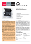
Acquire a Scout Image
Drag and drop a scout protocol onto the graphics canvas to accurately plan the target image.
The default scout protocol is based on a gradient echo sequence (gems) with a field-of-view
(FOV) of 100 mm, slice thickness of 2 mm, matrix size of 256x128, te=10, and tr=20. The
scout protocol acquires a single slice in each of the three cardinal panes in order: axial,
coronal, and sagittal. The scan takes a few seconds. Any image sequence may be used.
26
1.
Make sure the correct rf coil is selected – on the Prescan page of the Start tab.
2.
Go to the Plan viewport.
3.
Click the Plan button on the right side of the tool bar.
VnmrJ Imaging User Guide for VnmrJ 2.2B
01-999344-00 A 0207
2.1 Running a New Study
4.
Make sure the scout protocol is in the Study Queue.
Select the scout protocol in the Locator and drag it into the Study Queue if it is not
in the Study Queue.
5.
Load the scout scan by double-clicking it in the Study Queue or by dragging it to the
Plan viewport.
6.
Click on the Acquire tab to open the Acquire folder.
7.
Enter the appropriate settings in the Scan, Plan, and Advanced pages, see Figure 3.
The common parameters are on the Scan page. Image prescription and spatial
control are on the Plan page. Less common parameters and acquisition control is on
the Advanced page.
8.
Click Start Scan to run the scout protocol.
9.
Click on Current button to view the scout images as they are acquired.
Figure 3. Setting Up to Acquire a Scot Image
01-999344-00 A 0207
VnmrJ Imaging User Guide for VnmrJ 2.2B
27
Chapter 2. Running an Imaging Study
Shim the system after the scout images are acquired. The scout protocol moves to the top
when the acquisition is started if it was not the first protocol listed in the Study Queue.
Shimming
Global Shimming
Manual global shimming is necessary for experiments that do not use voxels (i.e., slice or
volume selective, the spuls protocol).
Acquire Scans
Run other protocols:
1.
Click the Plan button to open the Plan viewport.
2.
Click the Plan button in the upper right area of the screen.
3.
Drag the protocols from the Locator to the Study Queue.
Protocols can be acquired in any order, independent of their position in the Study
Queue.
4.
Verify the required protocols are listed in the Study Queue.
5.
Double-click on the completed scout scan in the Study Queue or any completed
imaging scans.
Select multiple completed scans for planning:
a.
Load the first scan by double-clicking the completed scan in the Study Queue.
This unloads any previously displayed images.
b.
Add other completed scans by dragging them into the graphics area.
6.
Double-click the protocol to execute and load the parameters into the parameter
page.
7.
Open the Acquire folder.
8.
Set the Scan parameters on the Scan page or set the detailed acquisition parameters
on the Advanced page.
9.
Plan the slices on the Plan page.
Refer to Chapter 6, “Interactive Image Planning,” for more information on image
planning.
28
VnmrJ Imaging User Guide for VnmrJ 2.2B
01-999344-00 A 0207
2.1 Running a New Study
10. Click Acquire Profile to see a readout projection.
11. Click Start scan to begin the scan.
A delay of several seconds from clicking Start scan until the sequence begins
acquiring is typical. This is due to calculations in the sequence and the downloading
of the acquisition instructions. Click Prepare to scan begin calculations before
starting the scan. Wait for completion of the calculations. Click Start scan and start
the scan will immediately. Start scan must be clicked after clicking on Prepare to
scan. The acquisition status field displays Ready when the calculations are
complete and the scan is ready to start.
12. Go to the Current viewport to view the images as they are acquired.
Protocols are shuffled up in the Study Queue as they are executed; acquired scans are listed
in the order of acquisition from the top of the Study Queue. Study data is saved
automatically as it is acquired.
The scan time shown for each protocol in the Study Queue is only updated when you select
the option Scan Time in the acquisition menu or when you click Start Scan. Scan Time also
executes the calculation part of the sequence and is a convenient way to check the
combination of parameters.
Continue to prepare and plan subsequent protocols in the Plan viewport while the current
scan is acquired.
Queue Scans
A series of scans may be queued and run in the Study Queue.
1.
Click the Plan button in the upper right area of the screen to open the Plan viewport.
2.
Add the protocols you want to run to the Study Queue.
3.
Queue scans individually.
a.
Double-click the protocol to queue.
b.
Customize any parameters.
c.
Click the Add to Queue button.
Protocols are shuffled up in the Study Queue as they are queued.
4.
Repeat step 3 for all scans to queue.
5.
Select Queue All from the Study Options menu to Queue all scans in the Study
Queue.
6.
Remove scans from queue individually.
a.
Double-click the protocol to remove from the queue.
b.
Click the Remove from Queue button.
7.
Select Unqueue All from the Study Options menu to remove all scans from the
queue all scans in the Study Queue.
8.
Click the Start Queue button.
01-999344-00 A 0207
VnmrJ Imaging User Guide for VnmrJ 2.2B
29
Chapter 2. Running an Imaging Study
The queued protocols are loaded one by one into the Current viewport and run in the
order in the Study Queue.
9.
Click the Current button in the upper right area of the screen to open the Current
viewport and view scans as they run.
10. Follow step 1 through step 5 to queue more scans in the queue while it is running,
11. Follow step 6 and step 7 to unqueue scans from the queue while it is running,.
Once a scan has started acquiring, it cannot be unqueued.
12. Do the following to review data while the queue is running.
a.
Click the Review button in the upper right area of the screen to open the
Review viewport.
b.
Double-click on the completed scan of interest.
Finish the Study
Click Clear Study in the Study Options menu and save the current study and start a new
study.
2.2 Creating Protocols
Protocols are predefined parameter sets. We distinguish between a basic protocol that
consists of a single parameter set (e.g., T2wt), and a composite protocol that is a collection
of basic protocols. Refer to Chapter 4, “Protocols for Imaging,” for detailed descriptions of
each imaging protocol. This section describes how to make protocols.
Making a New Protocol
1.
Load a protocol to use as a basis for the new protocol.
2.
Set the parameters in the current panel.
3.
Click on the Edit menu, select Create
Protocol, and select Make New
Protocol.
4.
Define the protocol attributes in the
New Protocol window,.
5.
Click Make protocol. If the protocol
already exists the button reads Update protocol.
Making a Composite Protocol
A composite protocol is a collection of basic
protocols with order information, ownership,
creation date, etc. A composite protocol does
not create new basic protocols, but instead
points to the selected basic protocols.
1.
30
Click on the locator
Sort Protocols.
and select
VnmrJ Imaging User Guide for VnmrJ 2.2B
01-999344-00 A 0207
2.3 Reviewing a Previous Study
2.
Drag one or more protocols into the Study Queue.
3.
Click on the Edit menu, select Create Protocol, and select Make a Composite
Protocol.
4.
Define the protocol attributes in the Composite Protocol window.
5.
Click on Make protocol. If the protocol already exists the button reads Update
protocol.
2.3 Reviewing a Previous Study
A previous study can be reviewed as follows.
1.
Make sure no scans are running.
2.
Click the Review button in the upper right area of the screen to open the Review
viewport.
3.
Select Sort Studies in the Locator. Click on the
the sort as necessary.
4.
Drag and drop the desired study from the Locator to the Study Queue to load the
study.
5.
Double-click on an acquired protocol node to load and view the data.
and select Sort Studies.Adjust
2.4 Continuing a Previous Study
A previous study can be continued and scans added to it by loading the previous study as
described above (Reviewing a Previous Study) and selecting the Continue study option in
the Study Options menu at the bottom of the Study Queue.
A previous study can be continued as follows.
1.
Make sure no scans are running.
2.
Click the Plan button in the upper right area of the screen to open the Plan viewport.
3.
Select Sort Studies in the Locator. Click on the
the sort as necessary.
4.
Drag and drop the desired study from the Locator to the Study Queue to load the
study.
5.
Select the Continue Study option in the Study Options menu at the bottom of the
Study Queue.
6.
Follow the procedures in “Acquire Scans,” page 28 or “Queue Scans,” page 29.
01-999344-00 A 0207
and select Sort Studies. Adjust
VnmrJ Imaging User Guide for VnmrJ 2.2B
31
Chapter 2. Running an Imaging Study
32
VnmrJ Imaging User Guide for VnmrJ 2.2B
01-999344-00 A 0207
Chapter 3.
Prescan
Sections in this chapter:
•
•
•
•
•
•
•
3.1 “Automated Prescan,” page 33
3.2 “Prescan Functions,” page 35
3.3 “Manual Prescan,” page 39
3.4 “Coil Table,” page 42
3.5 “Other Prescan Parameters,” page 44
3.6 “Setting Up and Calibrating 3D Gradient Shimming,” page 44
3.7 “Troubleshooting,” page 48
This chapter describes the prescan functions, their purpose, experimental setup, and
outcome.
The Start folder initially displays the Prescan page of the five pages: Subject Info,
Prescan, Prescan Adv, Prescan List and Prescan Setup in the Start folder.
3.1 Automated Prescan
Prescan is run in one of three automated modes that are selected on the Prescan pages:
•
•
•
“Full Prescan,” page 34 – A standard, full prescan.
“User List,” page 34 – You can define a list of prescan functions to execute in the
specified order.
“Single Prescan Mode,” page 34 – Execute any one of the above described prescan
functions.
Prescan returns to the target sequence and restores the imaging parameters selected at the
end of any of the automated prescans.
01-999344-00 A 0207
VnmrJ Imaging User Guide for VnmrJ 2.2B
33
Chapter 3. Prescan
Clicking the Prescan button in the Acquire action bar runs either a full prescan or the user
defined list, depending on whether the Use this list checkbox has been selected on the main
Prescan page.
Full Prescan
A full prescan is initiated either through the Prescan button on the Acquire action bar or
through the Full button on the main Prescan page.
A full prescan (default list) invokes the prescan functions in this order:
1.
Center Frequency
2.
Shim
3.
Center Frequency (repeated after shim)
4.
Power Calibration
5.
Receiver Gain
6.
Sequence specific prescan (if the sequence calls for it)
User List
1.
Click Use this list to run Prescan or Full using a user-defined
list of prescans.
2.
Click Modify to edit the list.
The button Clear List resets the list to an empty list The
Remove Last Item button removes the last list entry. Items are
added to the list by clicking the buttons under Add to Prescan.
The user defined prescan runs in the order specified by the user and
does not provide any checks or controls to ensure a meaningful
execution order.
Single Prescan Mode
Single mode prescan allows execution of individual prescan functions
in an automated manner. The operator can invoke any of the prescan
functions – frequency, shim, power, and gain – by clicking on the
respective button in the Run group on the main Prescan page.
Initializing Parameters for Prescan
There are three types of parameters used by the prescan routines:
•
•
•
Protocol parameters - saved in the.par file
Coil table parameters - saved in the Coil_Table file
Global parameters
The protocol related parameters can be modified in the Acquire page and saved in the.par
file by clicking on the Update params button. Most of the Coil_Table parameters
(related to the rf coil) appear in the Prescan Setup page and they are updated by clicking
on the Update button on that page. The Global parameters are not associated with an rf or
gradient coil so their values are used by the prescan routines until they are modified. Global
34
VnmrJ Imaging User Guide for VnmrJ 2.2B
01-999344-00 A 0207
3.2 Prescan Functions
parameters take precedence over the other parameters. The default parameters for the
prescan routines must be set correctly during installation of a new rf coil or else the prescan
experiments will fail. Most of the prescan parameters appear in the prescan setup page.
The prescan_init macro initializes the prescan parameters to default values. Enter a
value in the entry box corresponding to Set defaults and Pwr Limit to execute the
prescan_init macro. The power limit refers to the maximum power level (percent of
maximum) that will be used during the prescan power calibration routine
3.2 Prescan Functions
VnmrJ provides the prescan functions, frequency, power, shimming, and gain. A default
parameter set is initially loaded when running the frequency, power, or shimming prescan
functions. Such coil-specific parameters defined on the Prescan Setup page are updated
depending on the specific rf coil that is used.
A separate parameter set is not loaded when running the gain prescan function. The actual
scan parameters and pulse sequence is used.
•
•
•
•
“Center Frequency,” page 35
“Shimming,” page 36
“Power Calibration,” page 38
“Receiver Gain Adjustment,” page 39
Center Frequency
Center frequency prescan is designed to locate the main resonance frequency. Typically, it
is only necessary to perform this prescan once at the beginning of a study, or following any
changes in the shims.
The resonance frequency depends on the local field strength. Shimming of the magnet
shifts the frequency making it necessary to re-run center frequency after shimming.
Experimental Setup
The center frequency is determined using a non-selective pulse-and-acquire experiment.
The default parameters are in prescanfreq.par, and the coil-dependent parameters
that are set in the Prescan setup page are RF power, receiver gain, and a flag to specify a
slice selective frequency prescan. A 4ms sinc pulse is used, in the slice selective case, to
select the slice specified in the main Prescan page (orientation, offset, FOV, and thickness).
Result
The detected center frequency is stored in the global variable <tn>offset and used in all
subsequent scans, where <tn> is the observe nucleus. For example, when observing
protons, tn='H1' and the center frequency is stored in the parameter H1offset.
The frequency prescan routine also determines the frequency of fat as an offset relative to
water. The fat offset is stored in the global parameter Prescan_FatOffset.
Prescan_FatOffset defaults to 3.35 ppm if a fat peak is not detected.
The detection of the fat peak requires a reasonably good shim where the main (water) peak
does not show any slitting (single sharp peak), and the water and fat peaks are well
separated. Poor shimming can result in peak splitting and hence misinterpretation of the
spectra by the center frequency prescan. A fat peak is detected if the magnitude of the fat
01-999344-00 A 0207
VnmrJ Imaging User Guide for VnmrJ 2.2B
35
Chapter 3. Prescan
peak exceeds the fat threshold. The fat threshold is a percentage of the magnitude of the
water peak and can be adjusted on the Prescan Setup page (typically 5-10%).
Shimming
Shimming is a process of adjusting the local magnetic field to produce a homogeneous field
within the sample region. Two shimming methods implemented in VnmrJ: 3D image based
method (ge3dshim) and FID-shim (quickshim). The ge3dshim is based on field
mapping, a more advanced shimming techniques than quickshim, and allows a user to
shim on a selected sample region. It is particularly suitable for techniques that are sensitive
to field homogeneity such as localized spectroscopy and EPI. Setup procedures for
ge3Dshim are more complicated than quickshim and, depending on the application
and sample being used, is not usually recommended for routine (prescan) shimming
operations. The quickshim protocol is limited to global shimming involving only the first
order (x, y, and z) shims. It is a fast and simple method suitable for general shimming.
Shimming using 3D shim method require specification of the slice or voxel region for
shimming. This is done manually using the Plan page in the Acquire folder and a scout
image. Select either a voxel or a set of slices to bring up a button Save for shimming. Both
methods acquire data over a larger region, but only attempt to optimize the shims within
the specified shim region.
The 3D gradient shim method requires careful calibration of the shims, see, 3.6 “Setting Up
and Calibrating 3D Gradient Shimming,” page 44. A default parameter set for shimming is
first saved as described in 3.3 “Manual Prescan,” page 39. The shim parameters most often
changed by the user between iterations appear on the Prescan Setup page. The shimming
procedure is usually repeated multiple times with different shim parameters to improve the
field homogeneity.
The procedure for shimming is more complicated than for the other prescan functions.
Applications such as localized spectroscopy, CSI, EPI, etc. require different strategies for
shim optimization. Run the protocol in the interactive mode, see “Autoshimming
(Interactive Mode),” page 81, for these applications.
Experimental Setup for Quickshim
•
•
•
“Shim Calibration,” page 36
“Saving Parameters for Prescan,” page 37
“Prescan Shimming,” page 37
Shimming using either the Quickshim and 3D shim method require specification of the
slice or voxel region for shimming. This is done manually using the Plan page in the
Acquire folder and a scout image. Select either a voxel or a set of slices to bring up a button
Save for shimming. Both methods acquire data over a larger region, but only attempt to
optimize the shims within the specified shim region.
Quickshim requires calibrating the shim polarity and saving a default set of parameters for
use during the shimming procedure prior to using the Prescan shim routine.
Shim Calibration
The calibration step sets the polarity of the shim coils is done automatically on VNMRS
systems. Follow the "Shim Calibration" section described in the quickshim protocol for
other systems.
36
VnmrJ Imaging User Guide for VnmrJ 2.2B
01-999344-00 A 0207
3.2 Prescan Functions
Saving Parameters for Prescan
1.
Load the quickshim protocol.
2.
Set up the parameters as described in “quickshim,” page 102. Typical parameter
values are:
Parameter
Typical value
TR
30 ms
pw
10 µsec.
flip
4 deg
Data size
256
Spectralwidth
20,000 Hz
3.
Click on Acquire Spectrum button to obtain a spectrum and verify parameters.
4.
Click on the Save Prescan Params button to save the current parameters to the
parameter file:
~/vnmrsys/parlib/prescanquickshim.GCOIL.RFCOIL.par.
These parameters are associated with the currently selected gradient and rf coils. The
parameter defining the shim step size is set in the Prescan Setup page during the
prescan operation.
Prescan Shimming
1.
Select the Prescan page.
1.
Select the quickshim method for shimming.
2.
Click on Shim Settings button.
3.
Choose one or more iterations by selecting a check box.
4.
Specify a shim step value (del) for each iteration. Typically, set it to 500 to 200
DAC units for the first iterations and 100 to 50 DAC units for the final iterations.
5.
Click on the Shim button on the Prescan page to initiate Prescan shimming.
Previously saved experimental parameters are read in and the data acquisition
begins. The new x, y, and z shim values are determined and the hardware is updated.
During each shim cycle the shim settings corresponding to the maximum signal is
loaded.
6.
Click on the Shim button to repeat the shimming procedure if necessary.
Each first order shim is arrayed and a set of spectra are collected during the quickshim
procedure. The optimum shim value is determined by picking the largest peak. The shim
spectra are also displayed on the screen for diagnostic purposes.
Limitations
•
•
Shimming using the quickshim procedure is limited to first order shims.
The quickshim protocol uses hard pulses, so the whole sample area is chosen for
shimming.
Experimental Setup for 3D Shimming
1.
Prior to shimming save the default experimental parameters as described in 3.6
“Setting Up and Calibrating 3D Gradient Shimming,” page 44.
2.
Define the shim voxel or slices for shimming:
01-999344-00 A 0207
VnmrJ Imaging User Guide for VnmrJ 2.2B
37
Chapter 3. Prescan
a.
Acquire a scout image plan the voxel (for localized spectroscopy).
b.
Click on the Save Voxel for Shimming button in the Plan page to save it.
The region (slab) defined by the slices is used for shimming if slices are
planned. This step is not needed for global shimming.
3.
Choose the 3D option in the Prescan page for 3D image based shimming.
4.
Click on the Shim Settings button to view the shim parameters and display the
Prescan Advance page.
Set the following shimming parameters:
• The number of iterations
• Shim selection: 1st order (X,Y,Z), 1st and 2nd order, etc.
• Shim region: Voxel, Slab, or Global
• Tau (field encoding delay)
5.
Click the Shim button to start shimming. Previously saved experimental parameters
are read in, data acquisition started, and new shim values are calculated for the shim
region of interest. The procedure is repeated as necessary if multiple iterations are
chosen.
Result
Variation of the field the Shim region of interest is calculated after data collection. The shim
currents needed to minimize the field inhomogeneity are determined and the shim settings
updated using the shim calibration maps.
Power Calibration
Prescan power calibration calibrates the transmitter power for a 90 degree RF pulse.
Experimental Setup
The power calibration is determined using a profile in a slice-selective spin-echo
experiment (mems with a single echo), where the coarse RF power is set to a certain level
and the fine power arrayed.
The coil-specific parameters for the power prescan that are specified in the Prescan Start
page are TR, coarse RF power (enter the maximum coarse power for the 180 degree pulse),
and starting point, step size, and number of steps for the fine power array. Shown below the
entry fields is the actual range of power levels that will be sampled for the RF pulses. The
fine power array should be set up such that the profile intensity goes through both a
maximum and a minimum for the processing to work optimally. Otherwise a warning
message may be given.
The slice used for calibration is specified on the main Prescan page. Power prescan uses the
frequency prescan receiver gain.
Result
The power prescan fits the signal intensities to a second-order polynomial and uses the
maximum of this polynomial as the correct 90 degree pulse power setting.
The result of the transmitter power calibration is entered into the pulsecal file in the
user's local vnmrsys directory.
38
VnmrJ Imaging User Guide for VnmrJ 2.2B
01-999344-00 A 0207
3.3 Manual Prescan
Receiver Gain Adjustment
Receiver gain adjustment is the scaling of the receiver gain to ensure that the receiver and
ADC will not be overloaded during data acquisition.
Experimental Setup
The receiver gain needs to be adjusted using the exact pulse sequence and acquisition
parameters used for the target scan. There is no particular gain prescan sequence. The
execprescan macro is invoked, prior to executing the gain prescan, if the parameter
execprescan exists. This macro sets up the number of k-space lines acquired, steady
state scans, etc., to ensure a proper signal for the gain calculation. If execprescan does
not exist, only a single echo at the center of k-space is acquired (nv=0).
Result
Scaling is performed on the acquired FIDs collected during the execution of the selected
sequence. The gain prescan is designed to handle more than one echo or FID, in which case
the receiver gain is scaled to the largest echo or FID acquired.
The scaling will adjust the receiver gain in such a way that the signal is scaled to the
maximum receiver resolution multiplied by a gain scaling factor that is specified on the
Prescan Setup page (a typical value is 80% or 90%). A scale factor of 100% may result in
receiver overflow since the sampled echo / FID can vary slightly.
3.3 Manual Prescan
Manual prescan allows manual execution of either the center frequency, shimming, or
power prescan.
•
•
•
“Frequency,” page 40
“Power,” page 42
“3D Shimming,” page 40
The parameters for manual prescan are retrieved on the Prescan Adv page, Figure 4, by
clicking one of the buttons under Retrieve Data/Params.
Retrieve previous prescan data and parameter values
Figure 4. Prescan Adv Page
Saved data and parameters are retrieved, processed for inspection and subsequent manual
execution, if the prescan of choice is run as part of an automated prescan. Only the
predefined parameters are retrieved if the prescan has not previously been run.
01-999344-00 A 0207
VnmrJ Imaging User Guide for VnmrJ 2.2B
39
Chapter 3. Prescan
Frequency
Running the frequency prescan in the manual mode allows modification of the following
parameters on the Scan page in the Acquire folder: TR, RF pulse width, acquisition
bandwidth (sw), acquisition time, number of data points, transmitter power and offset,
receiver gain, and slice definition (orientation, offset, and thickness).
The Scan page, Figure 5, also contains buttons to manually Acquire and Process prescan
data.
The Update params button saves the current parameter set into the user's vnmrsys/
parlib directory, and any subsequent automated frequency prescan uses this parameter
set as a starting point.
The Return to Study button restores the original scan parameters.
Figure 5. Frequency Prescan Acquire Page
3D Shimming
The following section describes the procedure for setting up and running the 3D shimming
method interactively. The Manual Prescan mode allows the user to optimize and save a
parameter set for subsequent use in Prescan shimming. The Manual Prescan mode also can
be used to interactively shim the sample and to optimize parameters.
3D shimming setup and calibration are described in 3.6 “Setting Up and Calibrating 3D
Gradient Shimming,” page 44. For more details on the ge3dshim protocol, refer to
“ge3dshim,” page 67.
1.
Plan the region of interest (ROI) for shimming.
a.
Load a scout image and Plan a voxel or slice region prior to shimming.
The volume (slab) defined by the slice region is used for shimming if slices
are planned.
b.
Click on the Save for Shimming button in the Plan page to save the shim
ROI. This step is not required for global ROI shimming.
2.
Select the 3D shimming method in the Prescan page, see Figure 6.
3.
Load the 3D shimming parameters.
4.
Click on the Advanced button to open the Prescan Adv page, Figure 7.
5.
Click on the Shim button to load the default parameters.
The parameters are loaded from prescange3dshim_gcoil_rfcoil.par.
40
VnmrJ Imaging User Guide for VnmrJ 2.2B
01-999344-00 A 0207
3.3 Manual Prescan
Figure 6. 3D Shimming Prescan Page
Parameters from the system file, prescange3dshim.par are loaded if
prescange3dshim_gcoil_rfcoil.par does not exist.
Figure 7. Prescan Acquire Page for Shimming
6.
Click Acquire Profile to show a profile along the z-direction.
This can be used to check the experimental parameters such as the receiver gain and
SNR.
7.
Check and set the parameters. Refer to “ge3dshim,” page 67.
8.
Set the Shim parameters.
Choose the 1st or low order shims and use a short del value (field encoding delay)
if the initial field inhomogeneity is poor. Set parameters for multiple iterations if
necessary. A general strategy is to start with the low order shims with short del
values. Increase del and include the higher order shims as the homogeneity
improves.
9.
Click on the Shim button to start acquisition.
Do not click on the Start Scan button to initiate shimming. New shim settings will
be calculated and loaded after each iteration.
10. Save (optional) the default parameters for subsequent use by the Prescan-Shim
routine (see Section 2.2) by clicking on Save Params.
Note that when shimming during the Auto Prescan mode the Shim iteration
parameters mentioned in (step 8) are set from within the Prescan Advance page.
11. Optional: return to the previously loaded Study protocol by clicking on Return to
Study or by clicking on the protocol node in the study area.
01-999344-00 A 0207
VnmrJ Imaging User Guide for VnmrJ 2.2B
41
Chapter 3. Prescan
Power
Running the power prescan in the manual mode allows modification of the parameters.
Course or fine power array (starting point, step size, and number of steps) can be set up.
The buttons on the Scan page have similar functionality as for the frequency prescan with
the addition of a Display button that Fourier transforms the current data and displays the
data array.
3.4 Coil Table
The coil table is a text file containing important acquisition parameters for each rf coil.
Prescan will use the coil table to determine starting values for most of the functions and
automatically update the table if small changes, < 20%, occurred. The user is queried, to
accept or reject the update, if prescan detects the need for larger changes. The coil table file
(CoilTable) is located in the vnmrsys directory.
•
•
•
“Selecting a Coil,” page 42
“Adding or Modifying an RF Coil,” page 42
“Coil Setup,” page 43
The coil table contains 17 entries for each rf coil defined on the system.
Selecting a Coil
Select the rf coil on the Prescan or Prescan Setup page, Figure 8.
Page
Select coil
Prescan
Select the coil from the RF coil pull-down menu in the Hardware field.
Prescan Setup
Select the coil from the RF Coil pull-down menu in the Select Coil field.
Figure 8. Selecting a Coil on Prescan Setup Page
Adding or Modifying an RF Coil
42
1.
Click on the Start tab.
2.
Select the prescan panel.
3.
Click on the Modify Setup button.
VnmrJ Imaging User Guide for VnmrJ 2.2B
01-999344-00 A 0207
3.4 Coil Table
Add an RF Coil
1.
Click on the New entry button in the Select Coil region.
2.
Enter a coil name.
3.
Enter all required information in the Prescan Setup page fields.
4.
Click on the Save button.
Modify an Existing RF coil
1.
Select an existing coil from the drop down menu next to RF Coil.
2.
Enter all required changes in the Prescan Setup page fields.
3.
Click on Update.
Some knowledge or estimate of reasonable coil table values is required. If the coil table
values are unknown, starting values can be determined by entering conservative values
(i.e., low transmitter power and long TR's) and repeatedly running the prescans in the single
prescan mode, until a reasonable result is obtained.
Remove an Existing RF coil
1.
Select an existing coil from the drop down menu next to RF Coil.
2.
Click on Remove.
Coil Setup
Obtain prescan parameters for the power calibration as follows:
1.
Use a long TR (1000-2000ms).
2.
Enter the maximum power the RF-coil can handle without damage into the entry
field for power coarse in the Power Setting field. If value is unknown start with a
small coarse power setting (50 to 55).
3.
Set the following: fine power 100; Step size 100; and Number of Steps 22 for the
fine power.
4.
Click Power on the main Prescan page.
5.
Inspect the resulting spectra to ensure that there are at least three (3) points before
the maximum and at least four (4) points after the minimum.
Problem
Solution
Too few points after the minimum
Increase the number of steps or coarse power
Too many points after the minimum
Reduce coarse power or number of steps
Too few points before the maximum
Reduce the coarse or starting fine power
Too many points before the maximum
Increase the starting fine power
Multiple maxima
Reduce the coarse power
Minima is very close to the maximum
(less than four points apart)
Reduce the step size and possibly increase the
number of steps
6.
Click Update, every time parameters are changed.
7.
Repeat, until the power prescan completes successfully.
01-999344-00 A 0207
VnmrJ Imaging User Guide for VnmrJ 2.2B
43
Chapter 3. Prescan
3.5 Other Prescan Parameters
Other prescan parameters are set on the Prescan Setup page, in the General Settings
group.
SNR Threshold
Enter an absolute value for the SNR, below which the prescan functions
will return with an error. This could happen if, e.g., the RF coil is not
connected correctly or the RF amplifier is not turned on.
Fat Threshold
Enter a threshold for the signal intensity of the expected fat peak relative to
the size of the water peak. If no peak if found around the expected fat
frequency with a sufficiently large signal, the default value of -3.5ppm is
used.
Max Num of Tries
Enter a limit to the number of iterations allowed. The prescan functions
will attempt to iterate until a sufficiently large SNR is obtained, by
increasing the receiver gain and transmitter power.
Display Data
Check to display the frequency and power prescan data after it is processed
(in the Plan viewport). Receiver gain data or sequence specific prescan
data will not be displayed.
Log Events
Check to log of events during in the prescan_log file in the user's vnmrsys/
prescan directory for both troubleshooting and evaluation of the system
performance.
Cleanup
Check to ensure removal of temporary files created during prescan. It is
highly recommended to let the Cleanup checkbox checked, unless errors
occur, in which case the temporary files may explain the errors.
3.6 Setting Up and Calibrating 3D Gradient Shimming
This section describes how to set up and calibrate 3D gradient shimming. To run the 3D
gradient shimming, refer to “ge3dshim,” page 67. For information about running 3D
gradient shimming as part of prescan, refer to “3D Shimming,” page 40.
Acquiring Shim Calibration Maps
1.
Place a cylindrical bottle or sphere containing doped water in the center of the
magnet. The sample defines the region of interest for the autoshimming routines.
The shim field maps are measured in the sample region only; it is not possible to
shim outside this region.
Note: Make sure that the proper decctool file is loaded. The same decctool file must
be used for subsequent shimming because the gradient and the shim scaling (gain)
factors are set in decctool file. A copy of the decctool file will be saved in $home/
44
VnmrJ Imaging User Guide for VnmrJ 2.2B
01-999344-00 A 0207
3.6 Setting Up and Calibrating 3D Gradient Shimming
vnmrsys/gshimdir/decc_file.GCOIL.RFCOIL for future reference.
Load the same gradient calibration file (gcoil) when calibrating the shims and
during autoshimming.
2.
Shim the sample manually using the SPULS sequence and save the result in a file
named start (svs('start')).
Alternatively, use the Shim page, Figure 9, in the Start folder.
Figure 9. Manual Shim Page
3.
Set the frequency on resonance.
4.
Calibrate the rf power as usual.
5.
Load the ge3dshim protocol.
6.
Check and set the imaging parameters for 3D gradient shimming.
Set up the parameters as in a regular 3D gradient echo sequence (GE3D). The TR
and flip angles are chosen to maximize signal and minimize saturation effects.
Sagittal orientation is selected because the sample is usually extended along the z
axis. A larger FOV and size along the read dimension could be specified without
sacrificing scan time. The following parameters will result in a total scan time of
about 2 min. when TR is set to 50 ms. The parameters which are relevant for
shimming are displayed in the Shim, Acq, and Map pages of the Acquire folder.
Typical parameters:
tr
25-100 msec. tr must be sufficiently long to avoid the duty cycle limit
on the gradient and/or RF hardware and to avoid saturation effects.
flip
1-10 deg.
Matrix
64x32x32
orient
sagittal
te
2-4 msec
nt
2
The FOV (Field Of View) parameter is chosen to cover the sample used.
01-999344-00 A 0207
VnmrJ Imaging User Guide for VnmrJ 2.2B
45
Chapter 3. Prescan
7.
Set the parameters for mapping the shims in the Map page of the Acquire folder.
Shim selection
The shims to be mapped are selected from the shim
selection menu. For example, select 1-(XYZ) for 1st order
shims or 1&2 for 1st and 2nd order shims and so on. The
step size for calibrating the shims are defined in percent.
The step size for the 1st order shims will usually be a lower
because they are driven by the high power gradient
amplifiers (and not by the shim power supply unit). In the
example below, 1st order shims are mapped by setting a
shim DAC to a value approximately 5-10% of the
maximum shim DAC value. For high-power gradients,
(>40 G/cm) and shims, reduce the step size to about 1%.
Field encoding
delay
del refers to the delay for encoding the residual B0 field.
delref is chosen so that the phase change during that
period is within +/-180 degrees, i.e. no phase aliasing has
occurred during that period.
Intensity
threshold
Threshold is the intensity threshold, in percent, used in
analysis. All signals below this value will be ignored. This
is useful to avoid errors caused by poor SNR. The data with
the longer TE is used to determine the threshold map (or
mask). Shim set sensitivity is set in DECCTOOL
Typical Parameters:
8.
9.
Shim change (XYZ)
5-10% (about 1% for >40 G/cm)
Shim change (2nd order)
10-20% (1-2% for shim coils < 12 cm)
del
2-5 msec
delref
0.25 to 0.3 msec
Threshold
10-20%
Select the shims (1&2) to be mapped:.
1-(XYZ)
1st order shims
1&2
2nd order shims
1 2&3
1st, 2nd and 3rd order shims
1&z2
x,y,z and z2 shims
all
all shims
Check the profile and optimize the receiver gain.
10. Collect a test image and check the image quality and SNR.
11. Click the Test image button to collect and display the images.
12. Click on the Edit menu.
13. Select Create Protocol.
14. Select Make New Protocol.
The shim protocols can be recalled and used later during autoshimming.
Generating a Shimmap
1.
46
Click Acquire Shimmap to acquire the shimmap data.
VnmrJ Imaging User Guide for VnmrJ 2.2B
01-999344-00 A 0207
3.6 Setting Up and Calibrating 3D Gradient Shimming
The shim file, start, is loaded and data acquisition begins. Three data sets are
collected corresponding to tau=0, delref, and del for each of the shims
selected. The total scan time is:
total_scan_time = (no_of_shims_selected+1) * 3 * scan_time
scan_time is the acquisition time for a single 3D gradient echo data set.
All the data files (.fid and.fdf files) are saved in the directory:
$home/vnmrsys/gshimdir/data.
2.
Click Generate Shimmap to generate the shim calibration file in gshimdir/
calib directory. The shim maps are generated after data acquisition is complete if
the check box is checked.
Saving the Shimmap Files
The file, shimmap.GCOIL.<NAME>.f, contains the shim calibration field map. The
parameter file, shimmap.GCOIL.<NAME>.param is also generated at this stage.
<NAME> is specified by the user to identify the shimmap files. The above files are used by
the gs_calc macro to calculate the shim currents needed during auto shimming. The .f
and .param files are created in the user's local directory, $home/vnmrsys/
gshimdir/calib.
Copy shimmap files into the system directory /vnmr/gshimdir/calib if the are to
be used by other users.
01-999344-00 A 0207
VnmrJ Imaging User Guide for VnmrJ 2.2B
47
Chapter 3. Prescan
3.7 Troubleshooting
Turn on Display of prescan results as well as Log Events on the main Prescan page and
rerun the prescan that fails. Visual inspection of the spectra will often reveal the problem.
•
•
•
•
“No Water Peak Detected,” page 48
“No Fat Peak Detected,” page 48
“No 90 or 180 Degree Pulse Found,” page 48
“Odd Looking Power Calibration Curve,” page 49
No Water Peak Detected
The frequency prescan is usually very robust. There are only a few reasons why no water
peak is detected:
•
•
•
•
•
•
•
No sample in the coil
The coil is not connected
The RF amplifier is not turned on
Transmitter power too small
Pulse width too small
The spectral width is too small.
Defective hardware
Make sure that the equipment is turned on and that the coil is properly connected. Then run
frequency prescan again.
No Fat Peak Detected
The common reasons for not detecting a fat peak:
•
•
Poor shim, causing a poor separation and distinction between the water and fat peaks.
Secondary (additional) peaks. Repeat shimming and check the appearance of the
spectrum.
Frequency prescan does not detect the fat peak:
•
Reduce the Fat Threshold. Very small fat peaks might well be below the Fat Threshold
and therefore ignored by the prescan.
No 90 or 180 Degree Pulse Found
Generally, this is due to incorrect settings in the coil table or hardware problems. See
Chapter 1, “Setting Up an Imaging System,” for setting up the power calibration
parameters.
No 90º pulse found:
•
•
48
Improperly tuned RF coil — results in a very large power requirement for a 90º pulse.
More power is needed. If power limit is being approached, increasing the pulse width
in the default power prescan parameter set and rerun the prescan.
VnmrJ Imaging User Guide for VnmrJ 2.2B
01-999344-00 A 0207
3.7 Troubleshooting
Odd Looking Power Calibration Curve
The envelope of the profiles
is supposed to be a fairly
symmetrical and smooth
looking curve, as an example
shows.
A very asymmetric curve
could be due to saturation
effects or mistuning of the
coil. Try running the prescan
with a much longer TR, or
tune the coil. Setting the
power limit to a high value can also produce strange results. Always use lower power
settings when setting up for a new coil. Gradually increase the power limit.
01-999344-00 A 0207
VnmrJ Imaging User Guide for VnmrJ 2.2B
49
Chapter 3. Prescan
50
VnmrJ Imaging User Guide for VnmrJ 2.2B
01-999344-00 A 0207
Chapter 4.
Protocols for Imaging
Sections in this chapter:
•
•
•
4.1 “Imaging Protocols,” page 51
4.2 “Standard Sequence Options,” page 114
4.3 “Commands, Macros, and Parameters,” page 116
This chapter describes some pulse sequences for imaging available on Varian NMR
spectrometers. Familiarity with basic spectrometer operations; such as shimming and
tuning are assumed and not included in this chapter. More detailed descriptions of all
commands, macros, and parameters are in the online help VnmrJ Command and Parameter
Reference.
4.1 Imaging Protocols
• “ct3d,” page 51
• “epi,” page 52
• “fse3d,” page 60
• “fsems,” page 62
• “ge3d,” page 65
• “ge3dshim,” page 67
• “gems,” page 91
• “mems,” page 95
• “press,” page 96
• “profile1d,” page 100
• “quickshim,” page 102
• “scout,” page 104
• “se3d,” page 104
• “sems,” page 105
• “spuls,” page 106
• “steam,” page 108
• “tagcine,” page 110
ct3d
The protocol ct3d is a 3D experiment primarily used for microimaging. The ct3d
experiment allows for echo times in the sub-millisecond range because it uses a nonselective excitation, followed by phase encoding in all three directions and acquisition of
01-999344-00 Draft A Final_edits_011907
VnmrJ Imaging User Guide for VnmrJ 2.2B
51
Chapter 4. Protocols for Imaging
only a single data point. The ct refers to the constant time between the excitation and any
data point.
pe
pe2
pe3
ADC
te
Advantages of ct3d
The ct3d is well suited for high resolution imaging of small samples with very short T2,
such as polymers or solids.
Limitations of ct3d
Long acquisition time. The ct3d suffers even more so from a long scan time than se3d
because of the phase-encoding in all 3 directions. For example, with a tr of 100ms and a
matrix size of 32x32x32, the total scan time is about 1 hour.
Running the ct3d Sequence
Use a short tr (10ms) and a small matrix size (32x32x32) to reduce the scan time. You can
increase the image (digital) resolution by setting fn, fn1, and fn2 to, e.g., 128x128x128.
See the ge3d protocol ( “ge3d,” page 65) for a description of the image orientations.
ct3d is apptype='im3D'.
Options for ct3d
Click Show profile on the Acq page to obtain a profile of the object.
epi
•
•
•
•
•
•
“Advantages of EPI,” page 53
“Limitations of EPI,” page 53
“Running the Sequence,” page 55
“Options,” page 55
“Optimizing EPI,” page 58
“Processing of EPI Data,” page 60
EPI (Echo Planar Imaging) is a routine imaging application for very rapid collection of
imaging data and for functional MRI. EPI enables monitoring of changes occurring within
52
VnmrJ Imaging User Guide for VnmrJ 2.2B
01-999344-00 Draft A Final_edits_011907
4.1 Imaging Protocols
fractions of a second and is less affected by motion and flow-induced artifacts than other
imaging methods.
EPI
ss
ro
pe
EPI with diffusion
ss
ro
pe
Advantages of EPI
•
•
•
Rapid imaging data collection, typically 25-100 ms.
EPI is less affected by motion and flow-induced artifacts than other methods.
EPI is particularly advantageous in applications where a large number of images must
be acquired in a short amount of time, or for monitoring rapid changes within fractions
of a second, such as:
• Functional MRI (fMRI)
• Perfusion studies using bolus tracking
• Diffusion tensor imaging
• Time-course studies
Limitations of EPI
EPI images are prone to severe artifacts and is seldom used for routine or diagnostic work.
•
•
•
•
“Image Distortions,” page 54
“Low Resolution,” page 54
“Reduced Signal-to-Noise Ratio,” page 54
“Increased Gradient Requirements,” page 55
01-999344-00 Draft A Final_edits_011907
VnmrJ Imaging User Guide for VnmrJ 2.2B
53
Chapter 4. Protocols for Imaging
•
•
“Eddy Current Compensation,” page 55
“Oblique Slices,” page 55
Image Distortions
EPI echoes evolve as a function of time unlike the conventional spin-warp sequence. This
evolution means that if different resonances (e.g., oil and water) are present in the sample,
each of the echoes in the echo train is also chemical shift encoded.
Phase modulation caused by the chemical shift effect interferes with the phase correction
routines used to correct for the echo shifts along the T2-direction. The phase correction
routine that is used to calculate the phase maps is unable to distinguish the difference
between phase shift caused by incorrect alignment of echoes and phase shift caused by
chemical shift. Therefore, the phase-encode dimension represents both chemical shift and
spatial dimensions, which result in multiple images or ghosts corresponding to the different
chemical shift components in the sample.
Magnetic field susceptibility effects are a serious
limitation in EPI because they behave like
chemical shift effects. Susceptibility effects are
caused by either inhomogeneous fields in the
main magnet or susceptibility gradients caused
by the sample and other materials in the vicinity.
These effects are also phase encoded and appear
as frequency-shifted components in the phaseencode dimension, often leading to severe
distortions in the image. Therefore, shimming is
an important part of the EPI setup procedure.
Image distortions (ghost artifact)
Shimming on the slice should give better results than the usual single-pulse method. A
sequence such as profile1d can be used for shimming on the slice. When profile1d
is used, the echo or FID is detected after selectively exciting the slice region.
Susceptibility artifacts due to B0 inhomogeneity in EPI can be reduced by minimizing the
effective te and the total readout time. Several factors can accomplish this:
•
•
•
•
•
•
Minimum te option.
Multishot (for example nseg = 4, 8, 16) with a long tr and a couple of dummy scans.
Reduce the matrix size (nv and np).
Increase sw.
Use ramp sampling ON.
Linear k-space encoding may be somewhat superior to centric.
Low Resolution
The matrix size for single-shot EPI is usually limited to about 64x64 or 128x128 to keep
the data acquisition time short resulting in EPI images of low resolution. Higher resolution
images can be obtained through multi-shot EPI at the cost of increased total acquisition
time and possible artifacts.
Reduced Signal-to-Noise Ratio
Acquisition time following each excitation is typically 25 to 100 ms in an EPI experiment.
This significantly longer acquisition time than for conventional imaging sequences results
in images that are heavily T2* weighted, have a significant loss of signal, and yield images
with inherently lower signal-to-noise than conventional images of the same resolution.
54
VnmrJ Imaging User Guide for VnmrJ 2.2B
01-999344-00 Draft A Final_edits_011907
4.1 Imaging Protocols
Increased Gradient Requirements
Very strong and rapidly switching gradients are essential in EPI experiments to reduce the
acquisition time. The gradient hardware (gradient coil and gradient amplifiers) must deliver
high gradient strengths and short rise and fall times for the readout gradients.
Long gradient duty cycles and large gradients for relatively long periods of time
(particularly during time-course experiments) are required of the gradient hardware.
Eddy Current Compensation
Eddy currents create undesirable fields in the magnet region and result in image artifacts.
Actively shielded gradients and eddy current compensation hardware minimize eddy
current effects. Reducing the slew rate (increasing trise) reduces the eddy currents at the
cost of increased acquisition time and image distortions.
Oblique Slices
Oblique slices suffer from severe ghosting in EPI due to the current implementation of the
readout and phase encoding gradient waveforms,.
Running the Sequence
The epi sequence is a multi-slice, multi-shot, spin/gradient Echo Planar Imaging (EPI)
sequence.
Click on the Acquire tab and select the Advanced page to view or change the acquisition
and receiver parameters. The Direct Digital Receiver imposes certain limitations to how
closely spaced individual echoes can be acquired - error messages are generated if these
limits are violated. The following are typical settings for the receiver parameters:
•
Minimum echo spacing at least 100µs (spacing is automatically be increased if the
minimum is larger due to duration of phase encoding blips)
•
Time Correction off (primarily used for back-predicting FIDs to avoid artifacts from
digital filter rampup)
•
•
•
Data point size 16 bit
Sampling Rate 5MHz (first downsampling stage)
Filter Coefficients 5 (defines steepness of digital filters, which is typically not a
limiting factor in imaging)
The Advanced page has the buttons Test Scans, for acquiring a series of data sets with the
phase correction turned off (typically for debugging purposes), and Show RF & Grad, that
open up the RF pulses and Gradients pages containing all the information about RF pulses
and gradients used by epi.
The Prescan page has parameters for optimization of the sequence, described in more
details below. The epi sequence is apptype='imEPI'.
Options
•
•
•
•
•
•
Standard sequence options — see “Standard Sequence Options,” page 114
“Minimum TE,” page 56
“Multishot,” page 56
“Phase Encoding Scheme,” page 56
“Rampsampling,” page 57
“Navigator,” page 57
01-999344-00 Draft A Final_edits_011907
VnmrJ Imaging User Guide for VnmrJ 2.2B
55
Chapter 4. Protocols for Imaging
•
•
•
“Diffusion Weighting,” page 57
“Gradient Waveforms,” page 57
“Other acquisition parameters,” page 58
Option
Controlled by variable
Typical value
Automatic calculation of min TE
minte
'n' or 'y'
Repetitions, Time series
image and images
> 2
Multi-shot
nseg
1, 2, 4
Phase encoding scheme
ky_order
'l', 'c', 'lr' or 'cr'
Spin echo/Gradient echo
spinecho
'y' or 'n'
Ramp sampling
rampsamp
'y' or 'n'
Navigator echo
navigator
'n' or 'y'
Inversion Recovery
ir
'n' or 'y'
Diffusion weighting
diff
1 or 0
Fat suppression
fatsat
'n' or 'y'
Minimum TE
Selecting the TE Min check box (minte = 'y') forces the sequence to use the minimum
TE possible and updates the te parameter.
Repetitions
The number of repetitions controls the number of images acquired in a series of images (for,
e.g., bolus injection or fMRI). Repetitions must always be 2 or more, since the first data set
is a reference scan.
Repetitions uses the parameter images. Setting images>1 automatically arrays the
parameter image and sets the parameter image to 0,1,1,1,.... (with as many total elements
as images specify). Setting images=1 sets image=1. Actual image data is acquired if
image = 1. A reference scan (no phase encoding) is acquired if image = 0.
With images>1, the first acquired data set is not a proper image but rather a reference
scan. A phasemap acquired in this way is part of the total data set and is saved with the data.
Always set images >= 2 (the only exception is with diffusion, see below). If
images = 1, no phase correction is performed.
Manual manipulations the image array and intersperse zeros among the ones is possible
using the processing function (recon_all) to automatically use the most recently
acquired reference scan to phase correct subsequent image scans.
Multishot
The limitations of gradient strengths, resolution, and long acquisition times can be
overcome by running EPI as an interleaved, multi-shot experiment, where multiple EPI
echo trains are collected. Each of the echoes represents segments of k-space data and they
are combined to generate the complete k-space dataset during the post processing stage.
However, this type of experiment is no longer a single-shot method. The total scan time for
interleaved EPI sequences is increased by TR*nseg, where nseg is the number of
interleaved segments.
Phase Encoding Scheme
The order of which k-space is traversed (phase encoding direction) in multishot
experiments is given by the parameter ky_order.
56
VnmrJ Imaging User Guide for VnmrJ 2.2B
01-999344-00 Draft A Final_edits_011907
4.1 Imaging Protocols
ky_order can be either 'l' for linear or 'c' for centric ordering, or 'lr' and 'cr'
for linear and centric in the reverse directions. Linear ordering means that acquisition is
started at the edge of k-space, working towards k=0 and out to the opposite edge. With two
shots, each shot samples every 2nd line in k-space, with 3 shots, every 3rd line etc. Centric
ordering can only be used with an even number of shots; each shot starts at the center of kspace and works towards the edges, skipping nseg /2 lines if nseg > 2.
The sequence generates tables for phase encoding ordering on the fly. These tables are
found in the user's tablib, in a file that is named using the numbers nv, fract_ky, and
nseg, as well as lin for linear ordering or cen for centric ordering. Example, for
nv=128, fract_ky=64, single shot centric ordering: epi_nv128_f64_cen4
The tables are used for re-ordering of data prior to Fourier Transformation.
If the parameter pe_table exists (integer), it will be set to an array specifying the phase
encoding step ordering.
Rampsampling
Rampsampling refers to the acquisition of image data while the readout gradient is ramping
up or down, although skipping acquisition during the duration of the phase encoding blips.
The data is acquired in a non-linear manner, such that the dwell time between points may
differ on the ramp, but the gradient integral between points remains the same to ensure
constant steps in k-space.
Navigator
Check the Navigator check box on the Scan page to select a navigator echo. An extra echo
is collected with no phase encoding prior to acquisition of the actual image data. This echo
is used to correct for phase variations, typically caused by motion, throughout a series of
images.
Diffusion Weighting
Checking the Diffusion check box on the Scan page to turn on Diffusion Weighting. Go
to the Options page to specify the diffusion parameters see “Diffusion,” page 115.
The two diffusion gradients may be placed on either side of the 180 degree refocusing
pulse, or both before the 180 pulse, depending on TE. If TE/2 is very long (relative to
tDELTA, the separation of the diffusion gradients), they will be placed both before the 180
degree pulse. This can happen if the readout train and therefore TE is long.
Gradient Waveforms
The epi sequence uses the shaped gradient library to generate the following gradients, saved
in vnmrsys/shapelib:
Shape
Description
epiro
The entire readout train
epipe
All phase encoding blips, including zeros during acquisition
ror1
Initial readout dephaser
per1
Initial phase encoding dephaser
ss1
Slice selective gradient for excitation
ssr1
Refocusing of slice selective
ss21
Slice selective gradient for refocusing, if spin-echo option is selected
ssi1
Slice selective gradient if inversion recovery option is selected
01-999344-00 Draft A Final_edits_011907
VnmrJ Imaging User Guide for VnmrJ 2.2B
57
Chapter 4. Protocols for Imaging
Shape
Description
diff1
Diffusion gradients, if diffusion option is selected
crush1
Crusher gradient if fat saturation option is selected
These shapes are overwritten every time the sequence is executed (i.e., clicking on Scan
Time or selecting Show pulse sequence (dps) from the Acquisition main menu selection).
The displayed relative amplitudes of the shapes do not reflect their relative amplitude
during acquisition, they are all scaled to full amplitude (dac value 32767).
Other acquisition parameters
Additional parameters for all of the above options are shown in the Options page.
Optimizing EPI
Ideally all echoes appear at the middle of the acquisition window. Nonideal behavior of
gradients and spurious gradient fields (from local inhomogeneity and eddy currents, etc.)
influence the amplitude and phase of odd and even signals in differently. The echo positions
of the odd and even echoes shift increasingly away from the center of the acquisition
window throughout the echo train causing phase shifts between the odd and even echo
signals. Incorrect matching of odd and even echoes cause one of the more common and
artifacts in EPI images, half FOV ghosts. Half FOV ghosts appear along the phase-encode
dimension. The ghost image appears shifted from the primary image by half the FOV the
images. Shown in Figure 10 is an optimized image and a ghost image.
Well optimized
Image showing ghost artifact
Figure 10. Effects of Optimization of the Images Produced
Figure 11. Well-optimized Reference
58
VnmrJ Imaging User Guide for VnmrJ 2.2B
01-999344-00 Draft A Final_edits_011907
4.1 Imaging Protocols
Specific EPI imaging gradients must be optimized in order to compensate for non-ideal
gradients and minimize the ghosting. Gradient optimization accomplished by analyzing a
reference scan, see Figure 11 for an example of a well-optimized reference scan:
A reference scan is an entire dataset, but acquired with the phase encoding gradient turned
off. Thus, every single echo should in principle have the exact same phase and occur at the
exact same time, but due to gradient imperfections and local inhomogeneities, this is not
necessarily the case. The parameters groa, grora, and tep are adjusted in order to
ensure this condition.
These parameters are automatically adjusted, when you click the epi setup auto button.
Initially, the adjustment parameters are reset to all zeros, then a reference scan is done, from
which values for the adjustment parameters are calculated. Subsequently, a second
reference scan with new values is acquired and displayed. Several iterations of groa (for
horizontal tilt) and tep (for zipper effect, echo shift) are needed before they are optimized.
Click the buttons adj. tilt or adj. shift, respectively, to calculate new values and click epi
setup manual to acquire another reference scan with the new values. The data acquired with
either of these setup procedures is not saved with the study.
Examples of the reference scan and image with tep and groa incorrectly set are shown
in Figure 12.
EPI reference scan
with gradient delay
(tep) incorrectly
EPI reference scan
with groa
incorrectly set
Figure 12. Improperly Set values for tep and groa
The sample reference scans, see in Figure 12, small steps are noticeable from the first to the
second echo. This is primarily due to small, residual eddy currents that get into a steady
state after the first couple of lobes in the readout train. In order to force this steady state
before starting data acquisition, use the parameter ssepi to run a few gradient lobes identical
to the other readout gradients before starting acquisition.
01-999344-00 Draft A Final_edits_011907
VnmrJ Imaging User Guide for VnmrJ 2.2B
59
Chapter 4. Protocols for Imaging
Use the following adjustment parameters (on Prescan page in the Acquire folder) for this
EPI sequence:
Adjustment
Functionality
parameters:
For adjustment of
Typical values
groa
added to gro, G/cm
horizontal tilt
0 to 0.05 (positive or negative)
grora
added to gror, G/cm
vertical shift
1.0 (positive or negative)
tep
propagation delay, µs
zipper effect
0 to 100µs
ssepi
dummy gradients at
beginning of readout train
Step at the first one
or two echoes
1 to 2
Processing of EPI Data
The standard VnmrJ processing uses the recon_all function (see the Command and
Parameter Reference manual) and all settings are specified on the Recon page in the
Process folder.
•
•
“Phase Correction,” page 60
“Raw Data,” page 60
Phase Correction
Even after optimization, “Optimizing EPI,” page 58, phase variations throughout the data
set due to local field inhomogeneities may remain causing cause severe distortion and
ghosting. Use the unencoded reference scans (acquired when image=0) and compute a
phase map that is applied to each slice of the imaging data. Estimate the phase maps using
one of the following methods:
•
•
POINTWISE – Directly compute the phase of each point in each echo (default).
•
LINEAR – Fit the phase of each profile (normalized by the profile of the center echo)
to a linear model in a region of sufficient signal for each echo and extrapolate the
model to generate a point-by-point phase map.
•
•
QUADRATIC – Similar to Linear, but a second-order polynomial model is used.
PAIRWISE – Use even and odd echo pairs of the reference scan to generate a linearlyfit phase estimate correction and applied to only the even echoes of the imaging data.
CENTER_PAIR – Use even and odd echo pairs occurring at the center of the train to
generate 2 linearly-fit phase estimate (see Linear) correction and apply to even and odd
echoes in the imaging data.
Raw Data
Click on the Raw data page and select to view k-space data for a particular slice and array
element.
Note: Always save the data prior to running the manual preprocessing. Preprocessing
(echo reversal and petable reordering) may change the data structure such that
recon_all no longer produces correct images.
fse3d
•
•
•
60
“Advantages of fse3d,” page 61
“Limitations of fse3d,” page 61
“Running the fse3d Sequence,” page 62
VnmrJ Imaging User Guide for VnmrJ 2.2B
01-999344-00 Draft A Final_edits_011907
4.1 Imaging Protocols
•
“Options for fse3d,” page 62
The fse3d protocol is a 3D variation of the fsems protocol.
ss
ro
pe
loop etl
times
te/2
te/2
Advantages of fse3d
The fse3d is a good alternative to both the ge3d and the se3d experiments. It is much less
prone to susceptibility artifacts than ge3d, but much faster than se3d due to the segmented
data acquisition.
The fse3d is well suited for:
•
•
•
High-resolution T2-weighted images (long te, long tr)
Imaging of regions of high susceptibility
Scans where high signal-to-noise is critical
Limitations of fse3d
•
•
•
•
SAR
The fse3d experiment may be restricted by SAR limits.
Mixed Contrast
The contrast in an fse3d image is usually not a straight-forward T2- or T1-contrast.
Long Acquisition Time
Although the fse3d experiment is faster than the se3d, it is still a relatively lengthy
experiment, due to the long tr – typically in the order of 3-4 seconds – necessary to allow
the spins to return to equilibrium between excitations.
3D Limitations
The fse3d experiment suffers from the same limitations in terms of wrap-around and
limited extraction capabilities as ge3d ( “ge3d,” page 65).
ADC Overflow
Because the fse3d sequence uses non-selective pulses with a 90° flip angle in an almost
fully relaxed system, it is likely to cause ADC overflow. On animal systems, this can be
avoided by setting the parameter presig='h'.
01-999344-00 Draft A Final_edits_011907
VnmrJ Imaging User Guide for VnmrJ 2.2B
61
Chapter 4. Protocols for Imaging
Running the fse3d Sequence
The parameters specific to fse3d are the same as for fsems ( “fsems,” page 62):
Parameter
Description
Typical Value
etl
the echo train length
4 or 8
esp
the echo spacing (time between echoes)
10 to 20 ms
kzero
the echo that shall be assigned to the center of
k-space (values between 1-etl)
1 or 2
Preparation of the sequence results in the generation of a table for specification of the order
of k-space lines (see also “gems,” page 91). The name of the table is defined as:
fse<nv>_<etl>_<kzero>
The advantage of choosing a large number of echoes (large etl) is the obvious reduction
in scan time but at the expense of reduced signal-to-noise or image resolution. A lower
kzero value gives spin-density weighted images, while a larger kzero value gives
T2-weighted images.
Additional acquisition parameters, such as the rf pulse definitions, bandwidth, acquisition
time and number of dummy scans is set on the Advanced page. See “ge3d,” page 65 for a
description of the image orientations.
The sequence, fse3d, is apptype='im3Dfse'.
Options for fse3d
Acquire Profile
Click Acquire profile on the Advanced page to obtain a profile of the object.
This function temporarily sets the number of phase encode steps to zero (nv=0), which
signals to the sequence to acquire a single echo under the readout gradient but without any
phase encoding. This will acquire a profile for each echo in the echo train. Use cf to select
which echo in the echo train you wish to view and transform it, for example: cf=1 ft.
fsems
•
•
•
•
•
“Advantages of fsems,” page 62
“Limitations of fsems,” page 63
“Running the fsems Sequence,” page 64
“Options for fsems,” page 64
“Optimizing fsems,” page 65
The fsems protocol is a fast spin echo multi-slice experiment where you can select the
number of echoes in an echo train as well as decide which echo will be the center of
k-space.
Advantages of fsems
The fast spin echo is a faster experiment than the conventional spin echo because multiple
phase encode lines are acquired following each excitation.
Spin echoes are regenerated by applying multiple 180° refocusing pulses and minimizing
signal loss due to T2*.
62
VnmrJ Imaging User Guide for VnmrJ 2.2B
01-999344-00 Draft A Final_edits_011907
4.1 Imaging Protocols
ss
ro
pe
te/2
te/2
loop etl
times
The fast spin echo is well suited for obtaining high-resolution anatomical images in a short
scan time.
Limitations of fsems
•
•
•
•
“Specific Absorption Rate (SAR),” page 63
“Mixed Contrast,” page 63
“Artifacts,” page 63
“Long Acquisition Time,” page 64
Specific Absorption Rate (SAR)
Acquiring the data using multiple 180° pulses results in is a significant deposition of rf
power. On human imaging systems the can conflict with Specific Absorption Rate (SAR)
limits specified by the FDA. If the SAR limit is exceeded, the hardware will abort the
acquisition with the error message SAR limit exceeded.
Mixed Contrast
The signal in an fsems experiment is usually a mix of the spin echo produced by the
90°-180° pulse pair and the stimulated echo caused by non-ideal 180° pulses.
Consequently, the contrast in an fsems image is usually not a straightforward T2- or T1contrast.
The kzero parameter, which specifies the echo closest to the center of k-space, can be
used to change the contrast in images. For example, kzero=1 will give a spin-density
weighted image, while kzero=etl gives a T2-weighted image.
Artifacts
T2 decay creates a signal modulation that is distributed in k-space by the echo ordering
scheme as multiple fsems echoes are acquired per excitation pulse. This results in edge
replication, ghosting, or blurring. Another source of fsems artifact is the combination of
spin echoes and stimulated echoes that can be misaligned due to imperfect gradient areas
or other sources of phase variation, which can also result in edge replication, or banding.
01-999344-00 Draft A Final_edits_011907
VnmrJ Imaging User Guide for VnmrJ 2.2B
63
Chapter 4. Protocols for Imaging
Long Acquisition Time
Although the fsems experiment is faster than the conventional spin echo, it is still a
relatively lengthy experiment. The long tr is typically in the order of 3-4 seconds (3-5
times T1) and necessary to allow the spins to return to equilibrium between excitations.
Running the fsems Sequence
The parameters specific to fsems are listed in the following table:
Parameter
Description
Typical Values
etl
echo train length
4 or 8
esp
echo spacing (time between echoes)
10 to 20 ms
kzero
echo that shall be assigned to the center of k-space
(values between 1 and etl)
1 or 2
tep
propagation delay caused by gradient hardware.
50 to 100 µs
Preparation of the sequence results in the generation of a table for specification of the order
of k-space lines (refer to “gems,” page 91). The name of the table is defined as:
fsems<nv>_<etl>_<kzero>
The advantage of choosing a large number of echoes (large etl) is the obvious reduction
in scan time but at the expense of reduced signal-to-noise or image resolution. Changing
kzero will change the image contrast. kzero=1 gives spin density weighted images,
whereas a higher kzero value gives T2 weighted images
The parameter petable specifies which table is used for data ordering (see “gems,” page
91). Additional acquisition parameters, such as the rf pulse definitions, bandwidth,
acquisition time and number of dummy scans is set on the Acq page.
The tep parameter can be used to center the echo within the acquisition window. tep is
the position of the echo, in microseconds, from the center.
The fsems sequence is apptype='im2Dfse'.
Options for fsems
•
•
•
“Inversion Recovery,” page 64
“Show Profile,” page 64
“Steady-State Scans,” page 65
Inversion Recovery
The spin echo sequence can be preceded by an inversion recovery (IR) pulse. The IR option
is controlled through the checkbox on the Scan page; this sets the flag ir to 'y' or 'n'.
When IR is activated, the inversion time (ti) is entered on the Scan page.
Show Profile
Obtain a profile of the object by clicking Show profile on the Acq page.
This function temporarily sets the number of phase encode steps to zero (nv=0), which
signals to the sequence to acquire a single echo under the readout gradient but without any
phase encoding. This will acquire a profile for each echo in the echo train. To view all
profiles, enter flashc ft dssh. To view a specific profile, for example the second
profile, enter flashc ft(2).
64
VnmrJ Imaging User Guide for VnmrJ 2.2B
01-999344-00 Draft A Final_edits_011907
4.1 Imaging Protocols
Steady-State Scans
The parameter ssc is used to force the pulse sequence to run ssc number of times prior
to the actual experiment.
Optimizing fsems
Readout Gradient
Optimizing the readout gradient:
The readout gradient can be optimized through the parameter grof. It will be multiplied
onto the calculated readout dephaser and is typically within the range 0.99 to 1.01.
Set up an array of values and click Show Profile on the Acq page.
This acquires a set of profiles (one for each echo in the echo train) for each value of grof.
Use cf to select which echo in the echo train you wish to view and do the ft, for example:
cf=1 ft dssh. Select the best profile and set grof accordingly.
ge3d
•
•
•
•
•
“Advantages of ge3d,” page 65
“Limitations of ge3d,” page 66
“Running the Sequence,” page 66
“Options for ge3d,” page 67
“Options for ge3d,” page 67
The ge3d protocol is a 3D version of the gradient echo that allows you to obtain a true 3D
image in a short time. ge3d uses a selective rf pulse for excitation followed by phaseencoding in two dimensions and readout in the third.
ro
re
pe2
te
Advantages of ge3d
As is true for the 2D version, ge3d uses a single excitation pulse at a reduced pulse flip
angle so a shorter repetition time (tr) can be used, thus reducing the time necessary for
obtaining the image data.
The ge3d experiment is therefore very well suited for the following:
•
High-resolution 3D images with extraction of images in any of the cardinal planes
01-999344-00 Draft A Final_edits_011907
VnmrJ Imaging User Guide for VnmrJ 2.2B
65
Chapter 4. Protocols for Imaging
•
•
3D angiography (see angio3D protocol)
3D contrast agent enhancement studies
Limitations of ge3d
•
•
“Susceptibility Effects, Signal-to-Noise,” page 66
“Extraction Planes,” page 66
Susceptibility Effects, Signal-to-Noise
The ge3d experiment suffers from the same limitations in regards to susceptibility effects
and reduced signal-to-noise as the gems experiments (refer to “gems,” page 91).
Extraction Planes
It is only possible to extract slices from the 3D data in the cardinal planes, axial, coronal,
or sagittal.
Running the Sequence
Set sequence timing parameters (TE, TR, number of averages, number of dummy scans,
and pulse flip angle) and the FOV/slice parameters on the Scan page. Typical values for te
and tr are 3-5ms and 10-30ms (single-slice), while the pulse flip angle usually is in the
range 5-30°. A minimum TE and TR can be applied by checking Min TE and Min TR,
respectively. A minimum TR may cause a gradient duty cycle error.
The slice selective gradient is always applied in the second phase encoding direction (PE2),
i.e., it limits the extent of the sample in the second phase encoding dimension. The
thickness of the slice selective slab can either be given in mm or as a percent of the FOV in
PE2 (on the Plan page). The center of the slab always coincides with the center of the FOV
in PE2.
Additional acquisition parameters are set on the Advanced page. A page displaying the RF
pulse and gradient parameters can be brought up by hitting the button Show RF & Grad.
Select the Scan page to select the orientation (orient) of the 1st extraction (ROxPE) of 2D
slices from the 3D data. This orientation is automatically extracted upon completion of the
data acquisition. Further extraction in any of the cardinal orientations can be done on the
Extract page in the Image folder.
The following tables define which direction is assigned to readout, first and second phase
encode directions; this table is essentially identical to that for 2D imaging, where the slice
select direction has been replaced with a 2nd phase encode direction (see “gems,” page 91):
orient
Readout
Phase encode
Phase encode 2
Axial
Y
X
Z
Coronal
Z
X
Y
Sagittal
Z
Y
X
Consequently, the orientations extracted depend on the value of orient:
66
orient
RO x PE
RO x PE2
PE x PE2
Axial
Axial
Sagittal
Coronal
VnmrJ Imaging User Guide for VnmrJ 2.2B
01-999344-00 Draft A Final_edits_011907
4.1 Imaging Protocols
orient
RO x PE
RO x PE2
PE x PE2
Coronal
Coronal
Sagittal
Axial
Sagittal
Sagittal
Coronal
Axial
The ge3d sequence is apptype='im3D'.
Options for ge3d
•
•
•
Standard sequence options — see “Standard Sequence Options,” page 114
“Phase Encoding Rewinding,” page 67
“RF Spoiling,” page 67
Phase Encoding Rewinding
Because the spins are not allowed to return to equilibrium between excitations, it may be
necessary to rewind the phase introduced by the phase encoding gradient after acquisition
to achieve a steady state condition. With phase encoding rewinding (PE rewind), a gradient
of the same amplitude but opposite polarity of the phase encoding step is applied following
data acquisition.
Phase rewinding is controlled by the variable rewind, which can be set to 'y' or 'n'.
RF Spoiling
The short tr used in the gems sequence may cause image distortions due to a non-steady
state condition resulting in residual transverse magnetization. To alleviate this, gradient
pulses (for T1 weighting) or RF spoiling phase modulation (T2 weighting) and rf spoiler
pulses (Zur, Y., Magnetic Resonance in Medicine, 21, 251, 1991) are usually employed in
the pulse sequence to minimize such artifacts.
The RF spoiler is controlled by the parameter rfspoil, which can be set to either 'y' or
'n'.
ge3dshim
•
•
•
•
•
•
•
•
•
•
•
•
•
•
•
“Advantages of ge3dshim,” page 68
“Limitations,” page 69
“Acquiring Shimmaps,” page 69
“Generating Shimmaps,” page 70
“Sample Effects on Shimming,” page 70
“Choosing the Field of View (FOV),” page 71
“Setting the Optimal Data Matrix Size,” page 71
“Setting the Optimal Shim Step Size,” page 71
“Quick Procedure to Obtain Z2 Frequency Shift,” page 79
“Autoshimming (Interactive Mode),” page 81
“Saving Parameters as a Protocol,” page 84
“Shimming for Localized Spectroscopy,” page 84
“Shimming for Imaging,” page 85
“Monitoring the Progress During Autoshimming,” page 86
“Transmitter Frequency,” page 88
01-999344-00 Draft A Final_edits_011907
VnmrJ Imaging User Guide for VnmrJ 2.2B
67
Chapter 4. Protocols for Imaging
•
•
•
•
•
•
“Eddy Current Problem,” page 88
“Fat-Water Problem,” page 88
“Viewing Field Maps and Images,” page 89
“Omitting Shims from Calculations,” page 90
“Notes,” page 90
“References,” page 91.
ro
re
pe2
te
The GE3DSHIM method is an autoshimming method based on field mapping using a 3D
gradient echo sequence. The first part of the procedure involves measuring the field
produced by each of the shim coils using the GE3DSHIM protocol. The resulting field map
or shim map is used to determine the optimum shim currents for shimming a sample. A any
errors in the shimmap cause the shim current calculations and the shimming procedure to
fail. This section, using examples, describes the steps involved in generating and analyzing
the shimmaps.
The 3D gradient shimming routines are based on measuring the rate of change of phase
between two 3D gradient echo images taken at two echo times, te and te+del. The echo
time difference, del, causes a phase difference between the images as a result of residual
magnetic field (B0 inhomogeneity) within the sample. The frequency or field is determined
by calculating the rate of change of phase from the two images.
phase = arctan(I/R) (radians)
[Eq. 1]
where R and I refer to the real and imaginary components in the image.
The frequency is measured by calculating the rate of change of phase:
frequency = phase/tau (radians/sec)
[Eq. 2]
tau is the echo time difference between the two images.
The field, B, is directly proportional to the frequency:
frequency = γ*B
[Eq. 3]
γ is the gyromagnetic ratio (rad/sec/T)
Advantages of ge3dshim
•
•
•
68
GE3DSHIM is a fast and automated shimming procedure for imaging or spectroscopy.
Multiple iterations are supported.
Shimming over a user-defined sample region is supported.
VnmrJ Imaging User Guide for VnmrJ 2.2B
01-999344-00 Draft A Final_edits_011907
4.1 Imaging Protocols
•
Easy specification of the shim region of interest when planning slices for imaging or
voxels for spectroscopy.
•
•
Robust phase unwrapping improves the reliability of field measurements.
Works with all available shim coils.
Limitations
•
The problem of phase-wrap is a serious limitation.
A serious limitation of this approach is that the phase can only be measured from zero
to ± Π. Larger phase changes, > Π, cause aliasing or phase-wrapping. Additional
(phase unwrapping) routines are necessary to determine the true phase and frequency.
In the current implementation an additional dataset is collected. The use of this
additional field map was found to significantly improve the reliability of the field
measurement.
The phase change measured using equation (1) returns a value in the range of ± Π.
Phase changes greater than ± Π. cause aliasing or phase-wrapping and cannot be
directly measured from the experiment. All field mapping routines use an experimental
or data processing scheme to unwrap the phase and determine the true phase or
frequency. An additional dataset with an echo time set to te+delref is collected
where delref is a short delay in the order of 300 µsec. The phase change during the
field encoding delay, delref, must be less than ±Π. This is verified by viewing the
corresponding field maps.
•
•
The recommended matrix size is 64x32x32 complex points.
•
•
Any orthogonal orientation can be used for shimming once the shim map is obtained.
•
Selecting regions with poor SNR result in unreliable phase (or field) measurements.
This is avoided by setting an intensity threshold.
The orientation of the image must be set to sagittal when acquiring data for the shim
map.
The shims are not be updated if the shim limit exceeds 32K and the program aborts the
shimming process.
Acquiring Shimmaps
Follow the procedures in “Acquiring Shim Calibration Maps,” page 44 and acquire
shimmaps. The following steps are executed by the acquisition macros:
1.
Load the start shim file.
2.
Create the shimmap parameter file, shimmap.gcoil.param.
3.
Collect the base map datasets, base.1.fid, base.A.fid and base.B.fid
corresponding to echo times, te, te+delref, and te+del respectively.
Base map refers to the residual field within the sample.
4.
Select the shim coil and set the shim offset.
5.
Collect the shimmap datasets, shim.1.fid, shim.A.fid and shim.B.fid
corresponding to echo times, te, te+delref, and te+del respectively. (shim
refers to the name of the shim, for e.g. x1, y1, etc.).
6.
Reset the shim value.
7.
Repeat step 4 to step 6 for each of the shim coils selected.
01-999344-00 Draft A Final_edits_011907
VnmrJ Imaging User Guide for VnmrJ 2.2B
69
Chapter 4. Protocols for Imaging
Generating Shimmaps
Follow the procedures in “Generating a Shimmap,” page 46 and acquire shimmap data.
The following steps are executed by the acquisition macros:
1.
Generate the phase (.p) and magnitude (.mag) images from the base datasets.
base.1.fid =>
base.1.p, base.1.mag
base.A.fid =>
base.A.p, base.A.mag
base.B.fid =>
base.B.p, base.B.mag
2.
All signals (and noise) below a given threshold are ignored to improve the reliabilit.y
of the field measurements. The base.B.mag file is used to determine the signal
threshold. All signals below the threshold are set to zero and ignored in subsequent
calculations.
3.
Generate the phase difference images.
base.A.p - base.1.p =>
base.A.wf
base.B.p - base.1.p =>
base.B.wf
The phase difference images may show discontinuities due to phase wrapping.
4.
Determine the true phase images by unwrapping the phase.
base.A.wf, base.B.wf => base.f
5.
6.
7.
Generate the phase (.p) and magnitude (.mag) images from each of the shim datasets.
shim.1.fid=>
shim.1.p, shim.1.mag
shim.A.fid=>
shim.A.p, shim.A.mag
shim.B.fid=>
shim.B.p, shim.B.mag
Generate the phase difference images.
shim.A.p - shim.1.p =>
shim.A.wf
shim.B.p - shim.1.p =>
shim.B.wf
Determine the true phase images by unwrapping the phase.
shim.A.wf, shim.B.wf =>
8.
Remove the residual base field in the sample to obtain the field map generated by
the shim coil .
shim.f* - base.f =>
9.
shim.f*
shim.f
Repeat (4) - (7) for each of the shim coil selected.
10. Concatenate each of the shimmap files into a single file, shimmap.gcoil.f.
11. Generate FDF (.fdf) files for viewing purposes.
Sample Effects on Shimming
The gradient echo sequence is sensitive to field inhomogeneity. The magnetic susceptibility
gradients caused by the sample leads to signal loss from T2* effects. Select a suitable
sample and shim it well, using a shim method such as FID-shim or FASTMAP, prior to
starting the shim calibration experiment.
Use a sphere or a long cylindrical sample for calibration experiments. A spherical sample
is easier to shim than a cylindrical sample and results in a more homogeneous reference or
70
VnmrJ Imaging User Guide for VnmrJ 2.2B
01-999344-00 Draft A Final_edits_011907
4.1 Imaging Protocols
base field map. Sample defines the extent of the shim calibration maps and the region over
which the shim calculations are performed. Regions outside this region and below a
specified intensity threshold are ignored in the shim calculations. Use a spherical sample
for the mapping process if the shimming is to be performed primarily for head imaging. The
head must be positioned within the mapped region during the autoshimming procedure.
Use a cylindrical sample to map a larger region along the z-axis. The nature of
susceptibility field gradients at the air-sample interface depend on the geometry and
orientation of the sample with respect to the main field. Increasing the length of the sample
minimizes the effect of susceptibility effects at ends of the sample. Large field gradients
near the ends of the sample can make manual FID shimming difficult. Use a field mapping
technique, if available, and shim the central part of the sample before mapping the shims.
A large water sample may cause difficulty in tuning the probe due to sample loading effects.
Another limitation of large, conductive solutions, particularly at high field, is the signal
variations across the sample due to dielectric effects. Under these conditions it is preferable
to use a non-conductive material such as acetone. (Mineral oil is not recommended because
it contains two broad CH 3 and CH2 resonances.)
Choosing the Field of View (FOV)
Choose a FOV parameters (lro, lpe and lpe2) that covers the active region of the RF
coil in use. The FOV along the z-direction is selected to avoid aliasing of the image from
the region near or outside the ends of the RF coil. A typical RF coil extends along the zdimension. The preferred sagittal image orientation and readout direction applied along the
z-gradient allows collection of more data points to ensure sufficient digital resolution
without increasing the scan time.
Samples with a wide range of sizes are typically used in imaging. Collect separate
shimmaps for each range of sample sizes (e.g. mouse, rat, rabbit) to ensure sufficient digital
resolution in the shimmaps for improved reliability and accuracy in the autoshim analysis
routines.
Setting the Optimal Data Matrix Size
The optimum matrix size used for GE3DSHIM is 64 along the readout and 32 along each
of the phase encoding dimensions. Increasing the phase encode dimension size increases
the data acquisition time. Increasing the matrix size increases the data memory size and
processing time.
Setting the Optimal Shim Step Size
During the shim calibration step, each of the shim (DAC) values is offset by a known
amount and the field map (Ft) is measured. The field map includes the field produced by
the shim coil (Fs) and the residual field (Fb) within the sample. To obtain the field produced
by the shim coil the base field map (Fb) must be subtracted:
Fs = Ft - Fb
[Eq. 4]
The shim offset values are specified through the parameters, step-I to step-IV. Step-I, for
example, is the shim offset used for calibrating the x, y, and z shims and Step-II is the offset
for the z2 shims, etc. (The shim offsets for the 3rd and 4th order shims are specified in the
macro, gs_acqshimmap.)A small step size will result in lower sensitivity in the field
maps generated because of the small phase change induced during the phase encoding
delay. A large value can contribute to signal loss in the images due to T2* effects. The step
parameters must therefore be chosen based on the sensitivity of each of the shim coils. A
number of factors affect the sensitivity of the shims:
01-999344-00 Draft A Final_edits_011907
VnmrJ Imaging User Guide for VnmrJ 2.2B
71
Chapter 4. Protocols for Imaging
•
Efficiency (Gauss/cm/A) of the shim/gradient coil (refer to the manual on the shim/
gradient system)
•
•
Strength of the shim power supply driving the (higher order) shim coils
Gradient amplifier and the gain setting for the x, y and z shims in DECCTOOL.
Experimental Example
The system, Table 1, and experimental parameters, Table 2, used for generating the shim
calibration maps for this study are given below:
Table 1. System Components for the ge3dshim Example
Component
Description
System
4.7T (200 MHz)
Sample
58mm OD, 18 cm long plastic bottle containing doped water (T1 = 1s)
RF coil
63 mm ID birdcage coil
Gradient coil
Magnex 205/120/S, 120 mm ID, 40G/cm
Shim PSU
RRI 5 Amp
Gradient PSU
Copely Model 220, 200 Amp, 300V
Table 2. Parameters for ge3dshim Example
Parameter
Value
Shim gain in DECCTOOL
2%
Shim Step size for x,y,z, and z2 shims
1%
Shim Step size for xz and yz shims
2%
Shim Step size for xy and x2y2 shims
5%
Reference delay, delref
0.25msec
B0 field encoding delay, del
1msec (typical range 1 to 4 msec)
TR
20 msec (typical range 20 to 50 msec)
TE
4 msec (typical range 2 to 4 msec)
Averages
1 (typical range: 1 to 4)
A long cylindrical sample was used to map each shim coil within the entire rf coil. A scout
image was used to verify the sample position in the 12 cm gradient/shim coil. The sample
was shimmed manually (FID shim) using the 1st and 2nd order shims to about 25 Hz
linewidth and the shim parameters saved in the start file for use during the shim
calibration procedure.
Experimental parameters for collecting shimmaps using GE3DSHIM are shown in the Scan
and Acq pages. (The voxel information is not used.) The total scan time was about 10 min.
The delref and del delays were set to 250 µsec and 1 msec respectively. The x,y, and z
shims, for example, were mapped by offsetting shim values by 1% of the maximum (i.e.
32K x 0.01 DAC units). The other shim step sizes used in the study are shown in the Map
page.
72
VnmrJ Imaging User Guide for VnmrJ 2.2B
01-999344-00 Draft A Final_edits_011907
4.1 Imaging Protocols
The imaging parameters used for this study are shown in Figure 13.
Scan page
Acq page
Map page
Figure 13. ge3dshim Example Scan, Acq, and Map pages
Shimmap Generation
Prior to acquiring the shimmaps it is useful to acquire a test image, see Figure 14. The
image can be used to identify problems associated with sample positioning, SNR, aliasing,
receiver overflow, etc. and to setup and optimize the imaging parameters. Figure 14, is a
test image using the GE3DSHIM routine, showing sagittal (RO-PE1) planes. The intensity
variation in the images is caused by dielectric effects (high intensity near the center of the
sample) and RF field inhomogeneity.
Figure 14. Sagittal (RO-PE1) planes
01-999344-00 Draft A Final_edits_011907
VnmrJ Imaging User Guide for VnmrJ 2.2B
73
Chapter 4. Protocols for Imaging
Shimming the sample using only the first and second order shims is sufficient for most
imaging applications. The shim calibration is initiated using the Acquire shimmaps button
in the Acquire-Map page. The field mapping routine collects two datasets with echo time
values set to te and te+del. A small value of del (the field encoding time) causes small
phase changes resulting in low sensitivity (SNR) in the field map data. A large del value
can cause phase wraps and loss of SNR in the image due to T2* effects. In the present
implementation an additional (reference) dataset with an echo time of te+delref is
taken and used in the phase unwrapping routine to determine the true phase change. It is
assumed that no phase wrapping occurs during the period delref and it is usually set to
about 250µsec.
First the field variation within the sample is measured and is referred to as the base field
map. Then each shim coil is offset by a specific shim-DAC value and the experiment
repeated. The shim offset is specified using the parameters, Step-I to Step-IV. Because the
sensitivity of each of the shims vary it is necessary to specify different shim offset values
for each of the shims during the mapping experiment. The offsets for the x, y, and z, are
determined by the Step-I parameter. Similarly, Step-II (z2), -III (zx, zy), and -IV(xy, x2y2)
are used for the second order shims.
Three datasets are collected at echo times, te, te+delref, and te+del for each shim
calibration map. If the 1st and 2nd order shims are selected for shim mapping, a total of 27
datasets are acquired - 3 base datasets, 3x3 1st order shim datasets and 5x3 2nd order shim
datasets. The total data acquisition time is: 27xTRxNTxNVxNV2 (NT is the number of
averages and NV and NV2 are the number of phase encoding steps).
Shimmaps are calculated after data acquisition is completed if the Generate shimmaps
option is selected. Clicking on the Generate shimmaps button generates the base field map
and the individual shim field maps. During the shimmap calculations the field map
produced by each of the shims are generated as 3-dimensional (FDF) image files. The
image files can be viewed easily using the Acquire-Map panel and can help the user to
identify problems and to check the quality of the shimmaps. The base field map shows the
residual field variation across the sample and is shown in Figure 15 and Figure 16.
Figure 15. Sagittal planes from the (Base) Field Map
The regions near the ends of the sample show a large field variation indicating
susceptibility effects in these regions or higher order field inhomogeneity in the magnet.
The large field variations at the ends can cause signal loss in these regions in the resulting
images. During shim calibration experiments, offsetting the shim currents can add to the
base field further exaggerating the signal loss. The loss of signal at the edges will reduce
the size of the resulting field map. It is therefore necessary to shim the sample well before
proceeding with the calibration. The large field gradients at the ends can be minimized by
using a shorter RF coil and/or by using an extended sample. A spherical sample will also
help to avoid the end effect problem but it will also limit the size of the shimmaps along the
z axis.
74
VnmrJ Imaging User Guide for VnmrJ 2.2B
01-999344-00 Draft A Final_edits_011907
4.1 Imaging Protocols
Figure 15, sagittal planes from the (base) field map produced by the sample. Darker areas
correspond to negative values and the lighter areas to positive values. Signals below the
threshold value are ignored and represented by zeroes (gray background). The ends of the
sample show a large field variation (see also Figure 16) because the sample is extended
along the z-axis making it difficult to shim well over the whole sample.
Figure 16 shows the field variation along the z-direction. A line profile was taken along one
of the sagittal planes shown in Figure 15. The intensity axis corresponds to the phase
difference (∆P radians) between the two reference images taken with echo times te and
te+del. The frequency is calculated from the rate of change of phase, (∆P /del) radians/
sec. The field is directly proportional to the frequency (Equation 3).
Figure 16. Field Variation in z-Direction
Figure 17 through Figure 25 show shimmaps corresponding to some of the first and second
order shim coils. The shimmaps must be carefully inspected for any unusual patterns or
artifacts. The field maps should show a gradually varying three dimensional function with
sufficient SNR as shown in these examples. The parameters used for collecting the
shimmaps are listed in Table 2.
Figure 17, the z-shimmap. Sagittal planes taken from z1c.f.fdf file showing the field
variation produced by the z-shim coil.
Figure 17. Sagittal Planes from z1c.f.fdf file
Figure 18, line profile, from Figure 17, along the z direction shows a linear variation of the
z-shim field. The intensity axis represents the phase change (in radians) caused by the zshim coil. The smooth profile indicates good SNR.
01-999344-00 Draft A Final_edits_011907
VnmrJ Imaging User Guide for VnmrJ 2.2B
75
Chapter 4. Protocols for Imaging
Figure 18. Line profile from Figure 17, along z-Direction
Figure 19 Shimmap (z2c.f.fdf) corresponding to the z2 shim coil.
Figure 19. Shimmap (z2c.f.fdf) of the z2 Shim Coil
Figure 20 shows a line profile along the z-direction taken from Figure 19. When the z2 shim
is applied during the mapping experiment a frequency (B0) shift occurs causing the profile
to be offset along the vertical axis. A procedure for removing the B0 shift is described in
“Field drift and B0 shift caused by Z2,” page 79.
Figure 20. Line Profile Along the Z-Direction, from Figure 19
Figure 21, sagittal (RO - PE) planes taken from the 3D xz-shimmap.
Figure 21. XZ-Shimmap, Sagittal (RO - PE) Planes
76
VnmrJ Imaging User Guide for VnmrJ 2.2B
01-999344-00 Draft A Final_edits_011907
4.1 Imaging Protocols
Figure 22, line profile taken from one of the planes shown in Figure 21. The profile does
not appear smooth because it is not interpolated properly due to limited digital resolution
and should not be interpreted as low SNR.
Figure 22. Line Profile From a Planes Shown in Figure 21
Figure 23, sagittal (RO-PE1) planes taken from the x2y2 shimmap.
Figure 23. X2Y2 Shim Map Sagittal (RO-PE1) Planes
Figure 24, transverse (RO-PE1) planes taken from the x2y2 shimmap
Figure 24. X2Y2 Shim Map Transverse (RO-PE1) Planes
01-999344-00 Draft A Final_edits_011907
VnmrJ Imaging User Guide for VnmrJ 2.2B
77
Chapter 4. Protocols for Imaging
Figure 25, a line profile taken from the image shown in Figure 23.
Figure 25. Line Profile From Figure 24
Figure 26, the phase difference image, yz.B.wf.fdf, showing the phase wrap problem near
the ends of the coil. Notice the abrupt phase changes when the phase difference exceeds the
+/- Π limit, see also Figure 27.
Figure 26. Phase Difference Image, yz.B.wf.fdf
Figure 27, the line profile taken from Figure 26 illustrates the phase jumps. The phase
unwrapping routine, gsphasetofield, determines the true phase form this data.
Figure 27. Line Profile from Figure 26
Generating the Shimmaps
Clicking on Generate shimmaps generates the shim calibration map in the users home
directory, $home/vnmrsys/gshimdir/calib/shimmap.f.gcoil. An
additional copy of the file, shimmap.gcoil.f.date is also saved. Date is the date
when the file was created. The shimmap.gcoil.param file contains the parameters
which are used by the analysis routines.
Specifying an ID or name for the shimmap file in the Settings page is optional. The optional
string specified by the user are contained in the .f (shimmap.gcoil.ID.f) and
.param files.
78
VnmrJ Imaging User Guide for VnmrJ 2.2B
01-999344-00 Draft A Final_edits_011907
4.1 Imaging Protocols
The shimmap files are also copied to the system directory; /vnmr/gshimdir/calib,
if the user is vnmr1 (the system hardware administrator) and provides global access to these
files for shimming.
Field drift and B0 shift caused by Z2
The z2 shim offset can cause a zero order field shift (B0) resulting in a frequency shift of
the water resonance. This does not pose a problem in most of the shim coils used in the
animal imaging systems. The z2 induced zero order field shift can be a problem with larger
shim coils such as those used in human imaging and some older shim coil designs. These
coils require a few seconds or even minutes for the field to stabilize. The shim field must
stabilize before proceeding with field mapping experiments.
The z2-drift and z2-field shift can be quantified using the macros get_z2drift and
get_z2z0 as described in the manual under the Fastmap Protocol. After running the
get_z2z0 macro the file, z2z0.gcoil, contains the frequency shift (Hz) per shim
DAC offset. This value must be entered in the Settings page. The get_z2drift macro
generates the file z2drift.gcoil showing the frequency of the water resonance at
various times after setting an offset on the z2 shim. The shimmap acquisition macros,
(gs_acqshimmap and gs_acq1shimmap) include a delay of 10 sec (default)
whenever the z2 shim is changed for the field and shims to stabilize.
Quick Procedure to Obtain Z2 Frequency Shift
1.
Shim a sample (e.g. spherical phantom used for system tests) and obtain a single
pulse spectrum using the spuls protocol.
2.
Place the cursor on the line and set the reference frequency display to zero using one
of the following procedures:
• Process => Display => Reference line, Zero
3.
Save the current shim settings using one of the following procedures:
• Start => Manual Shim => Save Milestone
4.
Offset the z2 shim value by 1000 dac units in the Manual Shim page.
5.
Click on Acquire Spectrum.
6.
Move the cursor to the peak and record the cursor frequency (cr) displayed on the
screen, this value including its sign is the frequency shift.
7.
The z2 shift (Hz/DAC_unit) is given by:
z2z0 = frequency_shift/(z2_shim_offset)
z2z0 = cr/1000
8.
Enter the z2z0 value in the Acquire => Settings page in the ge3dshim protocol.
9.
Reset the original shims by retrieving the saved shim file:
Start => Manual Shim =>Retrieve Milestone.
Optional Zero Filling
Selecting the Zerofill option on the settings page, Figure 28, doubles the digital resolution
of the shimmaps by zero filling the time domain signal. The option is useful when working
with small voxels because it adds more data points to the characterization of the field
01-999344-00 Draft A Final_edits_011907
VnmrJ Imaging User Guide for VnmrJ 2.2B
79
Chapter 4. Protocols for Imaging
variation resulting in better analysis. Select Zerofill option prior to acquiring the shimmap
data. The file shimmap.gcoil.param is created when the shimmap is created.
Figure 28. Selecting Zerofill Option for ge3dshim
Use the following procedure for post acquisition zero filling if zero fill flag was not set prior
to data acquisition:
1.
Edit the file shimmap.gcoil.param and change the data size
from 64 32 32 1
to 128 64 64 2
2.
Select Zerofill.
3.
Click on Generate Shimmaps.
Acquiring a single shimmap
During the shim-mapping experiment it may sometimes be necessary to repeat the
measurement for a single shimmap. The following section describes the steps involved:
1.
Load a parameter set that was used to collect the original shimmap dataset, for
example, base.1.fid. The experimental parameters must be kept the same as
the parameters used in the original experiment.
2.
Select the map to be acquired, either the shim name or base, in the Map page.
3.
Change the shim step size if necessary.
Do not change any of the other acquisition parameters.
4.
Click on Acquire a map.
5.
Modify the shimmap.gcoil.param file if necessary to include the new shim
offset.
6.
Click on Generate Shimmap to regenerate the shimmap file.
Only the shim step size can be changed. Changing the shim step requires editing and editing
the new value in the file, $home/vnmrsys/gshimdir/calib/
shimmap.gcoil.param, prior to step 6. During step 2 a parameter file
shimmap_2.param is generated for reference and this file can be copied for use in step
5 as follows:
% cp shimmap_2.param $home/vnmrsys/gshimdir/calib/
shimmap.gcoil.param
80
VnmrJ Imaging User Guide for VnmrJ 2.2B
01-999344-00 Draft A Final_edits_011907
4.1 Imaging Protocols
Autoshimming (Interactive Mode)
The ge3dshim protocol is used for 3D gradient shimming. The Shim page of the Start
folder, Figure 29, contains the interface for shimming operations.
Figure 29. Interface for ge3dshim Shimming
The first step is to calibrate the shims, as described in 3.6 “Setting Up and Calibrating 3D
Gradient Shimming,” page 44. The shim DAC values are changed by a particular value and
the resulting 3D field map generated by each shim is calculated. During the shimming
process the B0 field is measured and the shim currents (DAC values) needed to minimize
the field are calculated and the shims updated.
3D autoshimming can be performed either in the Prescan mode or in the Interactive mode.
•
Prescan mode default parameters are predefined and initiated by the Shim button
during Prescan operations.
•
The interactive mode allows the user to intervene and control the shimming procedure.
The interactive mode is useful when encountering samples that are difficult to shim
because a cautious and step by step procedure may be necessary for optimizing the
shims.
Make sure that the DECCTOOL file and the gradient calibration files are the same ones
used during the shim calibration procedure described in the previous section before
proceeding with the autoshimming routines. The shim and gradient scaling (gain) are set in
the DECCTOOL file.
There is no generalized, universal procedure for autoshimming because the field
inhomogeneity is affected by the magnet and the sample itself. The protocol determines the
size and region that is shimmed making the interactive mode preferable to the prescan
option for shimming.
Multiple iterations of the autoshimming routines are sometimes requiring if the field
homogeneity is poor. A general approach to shimming under those circumstances is to start
shimming using the low order shims in a smaller region of interest (ROI) and then gradually
include the higher order shims while increasing the shim ROI.
Autoshimming can be done by a single button action. The number of shims, the shim ROI
and the number of iterations can be specified by the user. The region for shimming can be
specified by the user as:
Global
The region used for shim calculation is determined by the volume defined
by the field of view (i.e., lro*lpe*lpe2).
Voxel
The shim region is defined by the voxel parameters. This option is useful
for shimming a restricted area within a sample as in localized
spectroscopy. The voxel area can be specified by using the Plan routines.
01-999344-00 Draft A Final_edits_011907
VnmrJ Imaging User Guide for VnmrJ 2.2B
81
Chapter 4. Protocols for Imaging
Slab
The shim region is defined by the Slice parameters. In this case the
volume defined by the slices is used for shimming. For slab shimming,
the slices are specified by using the Plan routine.
Experimental Procedure
1.
Load the ge3dshim protocol into the Plan Viewport.
2.
Set up the parameters as in a regular 3D gradient echo sequence.
Note: The matrix size is usually set to 64 x 32 x 32, similar to the shimmap matrix size,
the FOV is chosen to cover the sample of interest, and the image orientation to an
orthogonal plane.
3.
Check the profile by clicking on Acquire Profile and optimize the receiver gain.
Set the gain lower in anticipation of an increase in the signal as the field
homogeneity improves.
4.
Set the transmitter frequency on the water resonance using Frequency-Prescan.
The frequency is set based on the field map calculations or by running the frequency
prescan measurement at the end of the shimming routine if one of the options to
update H1offset is checked in the Settings page,.
5.
Select the shims to be used for autoshimming. Only the shims that were mapped (see
“Generating the Shimmaps,” page 78) can be selected.
1-(XYZ)
1st order shims
1&2
1st and 2nd order shims
1 & z2
x,y,z and z2 shims
12&3
1st, 2nd, and 3rd order shims
all
all shims are selected
Reduce the del and delref values if the initial magnet field homogeneity is poor.
Longer del values can result in signal losses due to T2* effects. If in doubt collect
a 3D image (using Acquire Test Image) with te set to te+del and check the image.
Typical value for del is between 1 to 5 msec.An additional phase map is collected
using a much smaller B0 encoding delay, delref. delref is usually set to
about 0.25 to 0.5 msec and assumes the phase change during this delay is within
±180º.
6.
Select the region of interest for shimming:
Global
The region of the interest is defined by the Field of view parameters,
lro*lpe*lpe2 in the above case.
Voxel
Region of interest for shimming is done by planning a voxel using a
scout scan.
Scout image must be axial, sagittal, coronal, or one of the other
orthogonal planes. Display a scout image (by double clicking on a
previously collected scout image) and use the Plan page to Add a
voxel and define the voxel region of interest. Click the Save for
Shimming button to save the voxel information for use during the
shimming procedure.
82
VnmrJ Imaging User Guide for VnmrJ 2.2B
01-999344-00 Draft A Final_edits_011907
4.1 Imaging Protocols
Slab
Defining the volume containing the slices the region for shimming
when planning slices for imaging.
Planning slices while the currently loaded protocol is ge3dshim will
modify the FOV parameters. To avoid modifying the FOV
parameters, load the protocol to run, for example, GEMS or EPI. Plan
the slices using the scout image and save the slice volume information
by clicking Save for Shimming.
The shim ROI information is saved in the userdir/prescan/ directory. It will
be retrieved and used during the analysis by the gs_calc macro.
7.
Set Threshold (typically 10-20%) to avoid low signal-to-noise regions.
8.
Click Shim to start the autoshimming procedure.
9.
Check the Calculate Shims and the Load Shims options to calculate load new shim
values immediately after data acquisition without user intervention.
10. Click Calculate Shims to calculate the optimum shim settings.
Calculation results are written into the file in vnmrsys/gshimdir/data/
gshim.out. The results are also displayed Acquire-Analyze page, see Figure 30.
Figure 30. Shim Map Shim Calculations
11. Click Load Shims to update the shims.
Note: New shim values are not loaded into the hardware if any of the shim limits are
exceeded. Repeat the calculation (step 8) by choosing different shims and/or shimROI.
12. Verify the shimming results by running the SPULS protocol (for global shim) or a
localized spectroscopy sequence, e.g. PRESS, (for voxel shim). In the latter case the
spectrum must be taken from the same shim-ROI. It is convenient to run in the test
mode by clicking Acquire spectrum to collect and view the spectrum in the Plan
Viewport. If a larger shim ROI is chosen, use a gradient echo image of that region to
evaluate the progress in shimming.
13. Refer to “Monitoring the Progress During Autoshimming,” page 86.
Repeat step 8 through step 12 for shimming different ROIs or for experimenting with
different shim parameters using the data set acquired in step 7. Reduce the shim ROI and/
or use lower order shims during the iteration if the shim limits are exceeded.
The Load Shims option loads the new, calculated, shim values. Click the Restore Shims
button to restore the original shim values.
01-999344-00 Draft A Final_edits_011907
VnmrJ Imaging User Guide for VnmrJ 2.2B
83
Chapter 4. Protocols for Imaging
Setting up for Multiple Iterations
Each sample distorts the field differently. Interactively set the shim parameters and monitor
the progress of the shimming as described in the previous section. Up to 3 or 4 iterations
might be required to achieve optimum results. Automate the process for a given application
by setting up the parameters for multiple iterations.
The numbers of iterations required typically depends on the initial shim condition and
sample. Use shim settings corresponding to a spherical phantom of similar volume as a
starting point when shimming with an unfamiliar sample in the magnet.
Repeating the shimming procedure for convergence is usually necessary. Convergence is
experimentally verified in localized spectroscopy by checking the linewidth of the water
peak as described in “Shimming for Localized Spectroscopy,” page 84.
Start shimming in a small region using the 1st order shims if the initial field homogeneity
is poor. Gradually increase the size of the region of interest and include the higher order
shims.
Specify parameters for up to 4 iterations and press the Shim button to execute each shim
iteration automatically.
Setup for multiple iterations as follows:
1.
Select the shim parameters for each iteration.
2.
Click the check boxes above the selection can be used to enable the parameters. For
example:
Shim selection
1-(xyz)
1&2
1&2
12&3
Shim region
voxel
voxel
global
global
del (msec)
1.0
2.0
4.0
6.0
The initial voxel shimming is done using the first order shims with the del value set
to 1 msec. The second iteration is done using first and second order shims in the
same voxel region and with del set to 2 msec., etc.
3.
Press the Shim button.
Saving Parameters as a Protocol
To Save the current parameters as a protocol:
1.
Click on the Edit menu.
2.
Select Create Protocol.
3.
Select Make New Protocol.
4.
Save the ge3dshim protocol (or update if it already exists).
Shimming for Localized Spectroscopy
84
1.
Setup and save the Shim parameters (Protocol) as described in the previous section.
For localized spectroscopy, voxel selection should be chosen.
2.
Load, for example, the PRESS protocol.
3.
Setup the parameters for PRESS.
4.
Load the Scout image and plan the voxel.
5.
Save the voxel parameters (click Save for shimming).
VnmrJ Imaging User Guide for VnmrJ 2.2B
01-999344-00 Draft A Final_edits_011907
4.1 Imaging Protocols
During autoshimming the field inhomogeneity in the voxel region is measured and
the shims set accordingly.
6.
Collect a reference PRESS spectrum of water from the ROI and check its linewidth.
7.
Monitor the progress of autoshimming experimentally by following the changes in
linewidth of the water signal as follows.
8.
a.
Click on the Acquire Spectrum button to collect a spectrum in the Plan
viewport.
b.
Place the cursor line near the peak and click on Linewidth to obtain the width
at half height.
Load the ge3dshim protocol.
Set the parameters for autoshimming as described in the previous section on
Autoshimming. The Voxel shim region must be selected.
9.
Click the Shim button to shim the Voxel region.
The routines will collect the field maps, calculate the new shim values, and load the
shims.
10. Load the PRESS sequence from the study queue and check the linewidth of water as
in step 7.
11. Repeat step 8 and step 10 as necessary.
Shim using the first order (X,Y,Z) shims if the initial shim is poor and reduce the del value
to about 1 msec. Add the second order shims and increase the del value to about 2-5 msec
when the homogeneity is improved. Automate the procedure by setting up parameters for
multiple iterations.
Shimming for Imaging
Specify the slice region (slab) or the whole imaging volume (global) when shimming
during imaging experiments. Define the shim ROI using voxel parameters, see “Shimming
for Localized Spectroscopy,” page 84.
1.
Load the protocol to be run, for example, EPI, or GEMS.
2.
Using the scout image plan the slices for imaging as usual.
3.
Save the slice region (slab) for shimming by clicking Save for shimming.
4.
Do not plan the slice/slab region while the ge3dshim protocol is loaded. The FOV.
parameters will be modified if the ge3dshim protocol is loaded while planning the
slice/slab region.
5.
Defining the shimming region to be a voxel:
a.
Select a voxel regions such that regions of little interest are neglected in the
shimming process.
Avoid regions with large magnetic susceptibility effects, flow, motion,
chemical shift effects (e.g. fat signals, nasal and ear cavities when doing brain
imaging). These regions can lead to erroneous phase measurements.
b.
6.
Click Save for shimming.
Image planning is not necessary if global shimming is chosen. The whole field of
view region, lro*lpe*lpe2, in the shimming sequence (ge3dshim) is used as
the shim-ROI.
01-999344-00 Draft A Final_edits_011907
VnmrJ Imaging User Guide for VnmrJ 2.2B
85
Chapter 4. Protocols for Imaging
7.
Load the ge3dshim protocol from the study queue.
8.
Check and set the shimming parameters.
9.
Click the Shim button.
GE3DSHIM Procedure Summary
1.
2.
Acquire 3D datasets:
B0.1.fid,
∆te=0
B0.A.fid,
∆te=delref
B0.B.fid,
∆te=del
Fourier transform and generate the magnitude (.mag) and phase-angle (.wf) images:
B0.A.mag,
3.
B0.B.mag,
(Image B)
B0.A.wf,
(Phase A)
B0.B.wf,
(Phase B)
Unwrap the phase using the phase-angle images to give the true phase which is
proportional to the field.
B0.f
4.
(Image A)
(Acquired field map)
Reformat (re-grid) the B0.f data to match the shimmap file.
B0.rl.f
(field map)
5.
Use the shimmap data to calculate the shim currents needed to minimize the field
deviation and save the results in the text file: gshim.out.
6.
Load the new shim settings into the hardware.
Monitoring the Progress During Autoshimming
Shimming progress can be verified experimentally by checking the water linewidth (voxel
spectroscopy) or gradient echo image quality.
During autoshimming the file, userdir/gshimdir/data/gshim.out, gives some
useful information regarding the progress of shimming. The output can be viewed in the
Analyze page of the Acquire folder. During multiple iterations, the output will be saved in
the files, gshim1.out, gshim2.out, etc. A good indication of convergence is the change of
shim values listed in the gshim.out file. Another parameter is the RMS deviation given in
Hz. This parameter is a good indication of the NMR signal linewidth from the shim ROI.
86
VnmrJ Imaging User Guide for VnmrJ 2.2B
01-999344-00 Draft A Final_edits_011907
4.1 Imaging Protocols
Listing of the file gshim.out file
Shim
Change
........................
z0
-43
- frequency offset (Hz)
x1
-192
- predicted change in shim (DAC) values for the X shim
y1
13
z1
417
xz
-20
yz
166
z2
27
xy
1240
x2y2
1114
........................
B0 Field Map:
Matrix
- 64 32 32
FOV
- 25.00 16.00 16.00
Phasedelay - 8.00
Threshold - 1430601859072.0 x 10.0% -Maximum_Intensity x Threshold
........................
Shim Field Map:
Matrix
- 64 32 32
FOV
- 25.00 16.00 16.00
Phasedelay - 5.00
-B0 encoding delay, del
Number of shims mapped - 8
-No. of shim field maps measured
Number of shims defined - 8
-No. of shims used in calculations
........................
Shim Voxel Information:
Voxel shape: rectangular
Voxel dimension (pts)
- r=-31,31, p=-15,15, s=-15,15
- read, phase, and slice
Points in voxel(fraction)
- 3918/60543
-valid points within voxel/totalpoints
........................
B0 Field Map Statistics:
RMS deviation 6.67 Hz
-Measured field within the shim ROI
Peak deviation - 74.12 Hz
-Frequency range
........................
Calculated Field Map:
RMS deviation 5.70 Hz
-Predicted field after shimming
Peak deviation - 78.42 Hz
Listing of the file, shimmap.gcoil.param
The shimmap.gcoil.param file is saved in the userdir/gshimdir/calib/ directory,
when the shim calibration maps are generated. The file contains the parameters used when
the shim calibration maps were generated.
The shimmap and the corresponding parameter file are named shimmap.gcoil.ID.f
and shimmap.gcoil.ID.parm. The .ID refers to an optional user defined label for
identification purposes. It is specified in the Acquire-Settings page.
The number (1) in the MAP column of each row (shim) indicates the shimmap was
measured and included in the shimmap.gcoil.f file. A number in the ADJUST
column of each row (shim) is a flag to include (1) or exclude (0) a shim during
autoshimming.
01-999344-00 Draft A Final_edits_011907
VnmrJ Imaging User Guide for VnmrJ 2.2B
87
Chapter 4. Protocols for Imaging
#DATASIZE
64
32
32
1
Read, phae#1, phase #2, zerofill factor (1 or 2)
#FOV-MM
25
16
16
#DELAY-MSEC
5.0
B0 encoding delay, del
#THRESHOLD-PERCENT
10
#REFERENCE-DELAY-MSEC
0.5
#NO-OF-SHIMS
15
#SHIM
OFFSET
UNITS
MAP
ADJUST
x1
3200
DAC
1
1
y1
3200
DAC
1
1
z1
3200
DAC
1
1
xz
8000
DAC
1
1
yz
8000
DAC
1
1
z2
3200
DAC
1
1
xy
8000
DAC
1
1
x2y2
8000
DAC
1
1
x3
8000
DAC
1
1
y3
8000
DAC
1
1
z3
8000
DAC
1
1
xz2
8000
DAC
1
1
yz2
8000
DAC
1
1
zxy
8000
DAC
1
1
zx2y2
8000
DAC
1
1
Transmitter Frequency
Set the transmitter on the water resonance prior to starting the shimming routine. Small
frequency offsets (100Hz or less) are not going to cause a problem except when selective
excitation is used, see “Fat-Water Problem,” page 88.
During the shimming process the frequency of the water resonance shifts. The shift can be
significant for some systems when the Z2 and Z4 shims are adjusted. Selecting the option
Measure and Set Frequency on the Settings page to start the Prescan-Frequency routine
before each shim iteration and compensate for the field shift. Run the Prescan-Frequency
routing from the Prescan page to save the parameter set as a default for the current study.
Selecting the Calculate and Set Frequency option uses the field map information to
determine the frequency shift and set the transmitter frequency (H1offset). The Z0 value
in the gshim.out file refers to this frequency shift.
Eddy Current Problem
Pulsing the gradients causes eddy currents to be generated within the bore of the magnet.
The residual eddy current fields after compensation are usually negligible for most
practical applications but can be detected by field measurement experiment. Shimming
methods cannot distinguish between static field inhomogeneity and eddy current effects
erroneous shim corrections may be calculated. Eddy current effects can be cancelled by
setting nt=2. This doubles the total scan time. A general strategy might be to set nt=1
initially, when the field inhomogeneity is usually poor, and set it to nt=2 during the final
iterations.
Fat-Water Problem
Samples that do not include signals from fat in the shim-ROI (such as brain) do not require
fat suppression.
88
VnmrJ Imaging User Guide for VnmrJ 2.2B
01-999344-00 Draft A Final_edits_011907
4.1 Imaging Protocols
Shimming routines measure the phase changes from two images. The phase changes from
chemical shift effects in samples with two or more chemically shifted components (e.g. fat
and water) obscure the phase measurements. Limiting the fat signal is necessary during
autoshimming routines since water is used for mapping the field in imaging samples. Two
methods of limiting the signal from fat are:
1.
Selectively exciting the water signal with a soft pulse is a convenient way to limit or
avoid the fat signal. Excite the water selectively in the ge3dshim sequence by
changing the excitation pulse to a 4-10 msec. gaussian pulse and place the
transmitter frequency (H1offset) exactly on the water peak. The frequency-prescan
routines set the frequency on the tallest peak (typically the water peak). The longer
pulse length requires an longer te which can result in greater T2* signal loss.
2.
Select the Fatsat option on the Scan page of the Acquire tab.
Selecting this option allows the use of short and hard excitation pulses resulting in
shorter echo times.
Viewing Field Maps and Images
View the field maps generated by the shimming routines for debugging purposes. Field
maps produced showing artifacts the shimming routines do not work. All field maps are
generated in the vnmrsys/gshimdir/data/ directory. For example, z1.f.fdf contains
the field map produced by the z1 shim. Similarly, B0.f.fdf corresponds to the field map
generated during shimming. Load and view the field maps by typing the name of the file,
e.g. B0.f, and clicking Display image in the Map page or by clicking on FieldMap.
View the images. The 3 images collected during the fieldmap measurements are named,
B0.1.mag.fdf, B0.A.mag.fdf and B0.B.mag.fdf, corresponding to tau=0,
delref, and del respectively.
The field maps must appear as gradually varying functions. Any abrupt changes going from
positive to negative frequency indicates a phase warp. Reduce the del and repeat the
experiment if phase wraps appear within the shim ROI.
Low signal in the shim ROI indicates signal loss due to T2* effects — reduce the del,
te, and/or the threshold.
Click on Shim ROI (B0.mask.fdf) to view the shim ROI used in the fieldmap
calculations select the image. The image corresponds to the points which are within the
shim ROI and with intensities above the threshold level.
Select images using the image selection menu on the Analyze page. Phase A refers to the
phase-angle image corresponding to the echo time delref and Phase B refers to the
phase-angle image corresponding echo time del.The B0 field map is generated by
unwrapping the Phase B image.
Use the image selection menu on the Shim page to select the magnitude and phase-angle
images:
B0 map
acquired
B0.f.fif
∆te=del
Image B
Magnitude image
B0.B.fdf
∆te=del
Image A
Magnitude image
B0.A.fdf
∆te=delref
Phase B
Phase-angle image
B0.B.wf.fdf
∆te=del
Phase A
Phase-angle image
B0.A.wf.fdf
∆te=delref
Image Mask
Segmented shim-ROI
Test Image
Magnitude image
01-999344-00 Draft A Final_edits_011907
testimg.fdf
VnmrJ Imaging User Guide for VnmrJ 2.2B
89
Chapter 4. Protocols for Imaging
A B0 fieldmap acquired with FOV parameters that are different from the shimmap FOV
parameters are reformatted to match the shimmap data. Click on the Fieldmap button to
display the reformatted B0 map: B0.rl.f.fdf
Omitting Shims from Calculations
Edit the shimmap.GCOIL.param file in the vnmrsys/gshimdir/calib or /vnmr/
gshimdir/calib directory to ignore specific shims from the standard shim selection
option. This parameter file is generated when the shim calibration maps are acquired. The
following file was collected when the shim selection was set to 1&2. To ignore the x2y2
shim, set the MAP and ADJUST flags to 0 and click Generate Shimmap. Shim that are
not mapped are not used in shim calculations.
Listing of the shimmap.GCOIL.FOV.param file
#NO-OF-SHIMS
8
#SHIM
OFFSET
UNITS
x1
y1
z1
xz
yz
z2
xy
x2y2
3200
3200
3200
6400
6400
3200
6400
6400
DAC
DAC
DAC
DAC
DAC
DAC
DAC
DAC
MAP
ADJUST
1
1
1
1
1
1
1
0
1
1
1
1
1
1
1
0
Shimming on an Arbitrary Shim-ROI
Define an arbitrary region by using the ROI drawing tools. Select the roi option on the Shim
page to use the previously selected Shim-ROI for shimming.
1.
Click on the Acquire button and acquire a test image.
2.
Set the image orientation to Sagittal and the matrix size to 64x32x32 (the size is
similar to parameters used in the shimmap).
3.
Click on Display Test Image button on the Analyze page.
4.
Select the images to be used to draw the ROI using the MMB.
5.
Draw the region of interest using the ROI tools.
Draw the same or different ROI’s on the images selected.
6.
Click on Generate Shim ROI to save the ROI information.
7.
Select the roi shim region for shimming on the Shim panel.
Notes
90
•
Eddy currents can introduce additional field gradients. This can have an undesirable
effect on gradient shimming. Eddy currents are minimized by proper preemphasis
adjustments. Eddy currents can also be minimized by increasing the slew time of the
gradients and reducing the peak amplitude of the gradients.
•
Error messages from the C programs used in autoshimming are not printed in the
VnmrJ window. Select the window and enter the following to display the messages on
a specific shell window:
% tty
VnmrJ Imaging User Guide for VnmrJ 2.2B
01-999344-00 Draft A Final_edits_011907
4.1 Imaging Protocols
/dev/pts/6
Enter the following on the VnmrJ command line:
vnmrjcmd('tty','/dev/pts/6')
All VnmrJ related error messages, including those from the autoshim binary programs
will be printed in the above shell window. This is useful when debugging.
•
The ge3dshim.log is generated during the shim calculations and placed in the
directory: ~/vnmrsys/gshimdir/data/. Contained in the file is information on
the shim parameters and the intermediate files generated during the shim calculations.
The file is useful for trouble-shooting problems during autoshimming.
•
A minimum of three points are required along each axis to represent the field with a
proper pixel resolution. The pixel resolution in both the shimmap and B0 map must be
considered.
•
Reduce or start with a lower the receiver gain when doing multiple iterations. The
signal strength increases as the field homogeneity improves with each shim iteration.
•
The shim calculations will fail as a result of errors in the B0 field measurements arising
from phase wrap during the delref interval.
•
The shimming routine will fail if the SNR is not sufficient for accurate B0 field
measurements.
•
Collect individual shim maps for each sample size that will be used to insure sufficient
data points are used to represent the field changes over the shim ROI.
•
Set the transmitter frequency on the water resonance prior to running the gradient
shimming routine.
•
Check and set the transmitter frequency after loading a new set of shims. Z2 and Z4
shims tend to introduce a large B0 field component causing the resonance frequency
to be shifted.
References
P.Webb and A.Macovski, Magn. Reson. Med. 20, p113 (1991).
P.C.M. van Zijl, S.Sukumar, M.O.Johnson, P.Webb, and R.E.Hurd, J. Magn. Reson. Ser. A,
111, p203 (1994).
gems
•
•
•
•
“Advantages of gems,” page 92
“Limitations of gems,” page 92
“Running the sequence,” page 93
“Options for gems,” page 93
The protocol gems is a gradient echo 2D multi-slice acquisition technique. Common
variants of gems include FLASH™ (phase incoherent, T1 weighted) and GRASS™ (phase
coherent, T2* weighted). The gems protocol allows relatively fast acquisitions (less than 10
seconds per image) and short echo time (about 3 to 5 ms).
This protocol is provided as part of the Imaging _Sequences software accessory that
requires separately purchased license and password. If it doesn't appear in the Locator when
sorting protocols, install the Imaging_Sequences from the VnmrJ CD.
01-999344-00 Draft A Final_edits_011907
VnmrJ Imaging User Guide for VnmrJ 2.2B
91
Chapter 4. Protocols for Imaging
rf
gss
gro
gpe
ADC
te
Advantages of gems
A single excitation pulse is used in the gradient echo sequence and allows the use of a
reduced pulse flip angle and a shorter repetition time (tr). The data is acquired in less time
and high resolution images are obtained in a few seconds.
The gradient echo is therefore very well suited for the following:
•
•
•
scout scan
angiography (see angio protocol)
contrast agent enhancement studies
Limitations of gems
•
•
•
“Susceptibility Effects,” page 92
“Reduced Signal-to-Noise Ratio,” page 92
“Nonsteady-State Artifacts,” page 92
Susceptibility Effects
During the te delay, the spins are influenced not only by T2, but also susceptibility effects
resulting in rapid loss of phase coherence of spins in inhomogeneous regions (T2*).
Consequently, gems may suffer from signal loss and possibly image distortions in regions
of large susceptibility gradients. This is especially true at high fields.
T2* effects can be minimized by shimming or by reducing the te delay. Alternatively, the
susceptibility effects can be reduced by reducing the slice thickness and/or the pixel size
(i.e., increasing the matrix size or decreasing the FOV), since the loss of phase coherence
is directly related to phase variations within a pixel.
Reduced Signal-to-Noise Ratio
The use of a smaller rf flip angle and short tr in a gradient echo experiment results a lower
signal-to-noise than that of a spin echo experiment with similar experimental conditions
(see “sems,” page 105).
Nonsteady-State Artifacts
The short tr used in the gems sequence tends to cause a non-steady state condition
resulting in some residual transverse magnetization. Subsequent rf and gradient pulses can
92
VnmrJ Imaging User Guide for VnmrJ 2.2B
01-999344-00 Draft A Final_edits_011907
4.1 Imaging Protocols
generate stimulated echoes or other spurious signals that can severely distort the resulting
images. Crusher pulses (gspoil) and ro rf spoilers are used to minimize these artifacts.
Running the sequence
Set sequence timing parameters (te, tr, number of averages, number of dummy scans, and
pulse flip angle) and the FOV/slice parameters on the Scan page. Typical values for te and
tr are 10ms and 30ms (single-slice or 50-200ms for multi-slice), while the pulse flip angle
usually is in the range 5-30°. A minimum TE and TR can be applied by checking Min TE
and Min TR, respectively; however, be aware that minimum TR may cause a gradient duty
cycle error.
Additional acquisition parameters, such as the RF pulse parameters, receiver gain, and
crusher gradient amplitudes are set on the Acq page.
The correlation between image orientation and direction of gradients and the corresponding
Vnmr parameters psi, phi and theta is defined by the following matrix:
Readout
Phase encode Slice select
(psi,phi,theta)
Axial
Y
X
Z
(0,0,0)
Coronal
Z
X
Y
(0,0,90)
Sagittal
Z
Y
X
(90,0,90)
In 2D image display, the readout direction is always vertical, while the phase encoding
direction is horizontal.
Notice, that if the gradient coil has a low duty cycle, you may need to reduce the maximum
gradient allowed for refocusing and readout gradient by entering a smaller number for
Glim, typically in the range 30-75% (of maximum). In addition, you can reduce the spoiler
gradient by checking the Gspoil checkbox, thereby forcing it to use the value you can enter.
The gems sequence is apptype im2D.
Options for gems
•
•
•
•
•
•
•
•
Standard sequence options — “Standard Sequence Options,” page 114
“Flow Compensation,” page 93
“Phase Encoding Rewinding,” page 93
“RF Spoiling,” page 94
“Gradient Limitation,” page 94
“Spoiler Gradient,” page 94
“Table-Ordered Data,” page 94
“Show Profile,” page 94
Flow Compensation
Selecting Flow Compensation applies flow compensating gradients along both the readout
and slice select directions. This may increase the minimum TE.
Phase Encoding Rewinding
Because the spins are not allowed to return to equilibrium between excitations, it may be
necessary to rewind the phase introduced by the phase encoding gradient after acquisition
to achieve a steady state condition. With phase encoding rewinding (PE rewind), a gradient
01-999344-00 Draft A Final_edits_011907
VnmrJ Imaging User Guide for VnmrJ 2.2B
93
Chapter 4. Protocols for Imaging
of the same amplitude but opposite polarity of the phase encoding step is applied following
data acquisition.
Phase rewinding is controlled by the variable rewind, which can be set to 'y' or 'n'.
RF Spoiling
The brief tr used in the gems sequence may cause image distortions due to a non-steady
state condition resulting in residual transverse magnetization. To alleviate this, gradient
pulses (for T1 weighting) or RF spoiling phase modulation (T2 weighting) and rf spoiler
pulses (Zur, Y., Magnetic Resonance in Medicine, 21, 251, 1991) are usually employed in
the pulse sequence to minimize such artifacts.
The RF spoiler is controlled using the parameter rfspoil, which can be set to either 'y' or 'n'.
Gradient Limitation
Glim is a scaling factor on the maximum system gradient strength, which is applied to
refocusing, spoiler, and readout gradients. If the gradient coil has a low duty cycle, you may
need to reduce glim.
Spoiler Gradient
A spoiler gradient is always applied at the end of the sequence. Checking or unchecking
Gspoil does not disable this spoiler gradient, but rather enables user control of the spoiler
gradient amplitude. If Gspoil is unchecked, the maximum allowed gradient is applied. The
duration of the gradient, tspoil, is unaffected by the checkbox.
Table-Ordered Data
It is possible to acquire data from gems in nonmonotonic order by using an external AP
table to control the order. The table is selected through the parameter petable. If petable is
the blank string or the letter 'n' or 'N', no table is used and the data is acquired in monotonic
order. If petable is a non-empty string, e.g., petable='gems128', the sequence will
use the table in the file gems128.
The table file must include the table t1 which much contain as many integers as there are
phase encode steps in the protocol, ranging from -nv/2 to nv/2, however in arbitrary order.
The integers determine the order of the phase encoding steps.
Using a table allows you to play out the phase encode gradients starting from the center of
k-space (centric ordering) or specify partial k-space acquisition.
Show Profile
A profile of the object can be obtained by clicking the button [Acquire profile] on the Acq
page. This function temporarily sets the number of phase encode steps to zero (nv=0),
which signals to the sequence to acquire a single echo under the readout gradient but
without any phase encoding. The above matrix defines which axis to acquire the profile
along (readout). For example, to obtain a profile along Y, select axial, for a profile along Z,
select coronal. Since none of the predefined orientations have readout along X, you must
select axial and manually set phi=90 (on the Plan page) in order to get a profile along X.
94
VnmrJ Imaging User Guide for VnmrJ 2.2B
01-999344-00 Draft A Final_edits_011907
4.1 Imaging Protocols
mems
•
•
•
•
“Advantages of mems,” page 95
“Limitations of mems,” page 95
“Running the Sequence,” page 96
“Options for mems,” page 96
The mems protocol is a multi-echo experiment, where a series of spin echoes are acquired
following a single excitation. Each echo is acquired following a 180° pulse, resulting in a
series of images with increasing echo time that can be used for quantitative T2
measurements.
ss
ro
pe
loop ne times
te/2
te/2
Advantages of mems
The mems sequence allows you to sample a number of echoes with increasing echo time
following a single rf excitation. The data is subsequently sorted such that all phase
encoding lines acquired at a certain echo time are used to produce an image with a certain
effective te.
The mems sequence is primarily used to obtain multiple images with increasing te for
quantitative measurement of T2 in a relatively short time.
Limitations of mems
•
•
“Long Acquisition Time,” page 95
“Artifacts,” page 95
Long Acquisition Time
The primary limitation of the mems (and sems) sequence is the long scan time.The spins
must return completely to equilibrium in order to maintain the T2-weighted contrast and
avoid ghosting. A typical tr in the order of 3-4 seconds results in a total acquisition time
in the order of minutes for high resolution images.
Artifacts
Artifacts caused by the interference of the spin-echo and stimulated echoes affect the mems
sequence. Crusher pulses are usually applied to eliminate the spurious signals.
01-999344-00 Draft A Final_edits_011907
VnmrJ Imaging User Guide for VnmrJ 2.2B
95
Chapter 4. Protocols for Imaging
Running the Sequence
Set TR on the Scan page, typically in the order of 3000 ms, or select Min TR for
calculation of the minimum TR value.
The echo times can either be set manually or automatically to the minimum possible. The
Min TE checkbox sets the first echo time, TE, to the minimum. The Min ESP checkbox
calculates the minimum spacing between the first and second echo, and sets the second
echo time, TE2. If the EQ-ESP checkbox is checked, the echo spacing between echoes two
and three, three and four, etc, are automatically set equal to the spacing between echoes one
and two. Notice, that the first echo time, TE, is not the same as the echo spacing. The first
echo time is the Vnmr parameter te, whereas subsequent echo times are defined as an
arrayed parameter, te2.
An unfortunate side-effect: When manually defining echo times, it is possible to get into a
situation where the minimum echo time reported by the sequence appears to get longer and
longer, every time you enter a new value. This is related to a re-calculation of the
acquisition bandwidth and thus acquisition time, based on the minimum TE.
Specify a thk/thk2 ratio when defining the FOV and slice parameters. thk/thk2 it the ratio
of the thickness of the excitation (90º) pulse to the subsequent refocusing (180º) pulses.
Additional acquisition parameters, such as the rf pulse definitions, bandwidth, acquisition
time and number of dummy scans are set on the Acq page.
The mems sequence is apptype im2D.
Options for mems
•
•
•
•
Standard sequence options — see “Standard Sequence Options,” page 114
“Flow Compensation,” page 96
“Gradient Limitations,” page 96
“Show Profile,” page 96
Flow Compensation
Selecting Flow Compensation applies flow compensating gradients along either the
readout or the slice select direction, or both. Notice, that this in turn may increase the
minimum TE.
Gradient Limitations
Glim is a scaling factor on the maximum system gradient strength applied to refocusing,
spoiler, and readout gradients. Reduce glim for gradient coils with a low duty cycle.
Show Profile
A profile of the object at each echo time can be obtained by clicking the button Show
profile on the Acq page. This function temporarily sets the number of phase encode steps
to zero (nv=0), which signals to the sequence to acquire a single echo under the readout
gradient but without any phase encoding. By default, it displays the profile for the first echo
time. View the subsequent profiles by entering the command cf=<echo number> ft,
or all of them at once by entering flashc ft dssh.
press
The press protocol is used to obtain a 1D NMR spectrum from a localized region, with or
without water suppression. press is based on a double-spin echo.
96
VnmrJ Imaging User Guide for VnmrJ 2.2B
01-999344-00 Draft A Final_edits_011907
4.1 Imaging Protocols
vox 1
vox 2
vox 3
te1/2
•
•
•
•
te1/2
te2/2
te2/2
“Advantages of press,” page 97
“Limitations of press,” page 97
“Running the Sequence,” page 97
“Water Suppression,” page 98
Advantages of press
The press experiment offers higher sensitivity advantages over the steam experiment.
Limitations of press
Outer Volume
Contamination
The three slice selective pulses not only excite signals within the
voxel, but also regions within the slice plane. Imperfections in the
pulses result in unwanted signals in the transverse plane, which can
lead to artifacts in the spectrum. Carefully placed crusher pulses can
be used to destroy the undesired signals. An eight pulse phase cycling
scheme is used in press to cancel out the unwanted signals and
minimize artifacts in the spectrum.
J Modulation
The evolution of spins in the transverse plane causes the phase of the
J-coupled spins to modulate as a function of te and te2. This may
result in a spectrum that cannot be easily phase corrected.
Running the Sequence
1.
2.
Load the sequence and adjust parameters:
a.
Load the press protocol from the Study Queue.
b.
Load a scout image and define the voxel ROI using the Plan page.
c.
Set the echo times on the Scan page.
d.
Select the Advanced page to set additional parameters, including spectral
width (sw), acquisition time (at), and number of data points (np).
Acquire a spectrum and reference the water peak:
a.
Click Acquire Spectrum on the Advanced page to acquire a non-suppressed
test spectrum. This acquires and displays a spectrum without adding an entry
to the Study Queue. Use this spectrum to reference the water to 4.7 ppm.
b.
Position the cursor exactly on the water peak.
01-999344-00 Draft A Final_edits_011907
VnmrJ Imaging User Guide for VnmrJ 2.2B
97
Chapter 4. Protocols for Imaging
c.
Click Set water reference.
3.
Repeat step 1 and step 2.
4.
Click Set freq at cursor to set the transmitter frequency on the water peak.
5.
Set the receiver frequency to center the spectrum on, for example, water:
a.
Click Acquire Spectrum on the Advanced page to acquire a non-suppressed
test spectrum.
b.
Position the cursor exactly on the water peak.
c.
Click Receiver ref under the header Offsets on the Advanced page.
Clicking Set freq at cursor sets the global transmitter frequency, H1offset, at the cursor
location. The offset displayed with Receiver ref is an offset relative to the transmitter offset.
Start Scan automatically sets the receiver frequency (tof) to the correct absolute
frequency.
The outer volume contamination can be reduced by applying a crusher gradient. The
amplitude (gcrush) and duration (tcrush) are set under Crushers on the Advanced
page; they are referred to as te crushers and are typically set to 1-3G/cm and 2-5ms.
The phase cycling scheme consists of 8 steps.
The press sequence is apptype='im1D'.
Water Suppression
Water suppression is achieved by applying a selective RF pulse at the water frequency
followed by a spoiler gradient. Three water suppression methods are available:
•
•
•
WET
VAPOR
DRY
Water suppression is activated through a check box on the Scan page; this sets the flag
ws='y'. To set the water suppression frequency (wsfrq) on the water resonance:
1.
Click Acquire Spectrum on the Acq page to acquire a non-suppressed spectrum.
2.
Position the cursor exactly on the water peak.
3.
On the Advanced page, click Suppression under the header Offsets.
The DRY water suppression scheme is a CHESS method (Moonen et al, JMR 88, 28, 1990),
consisting of three consecutive rf pulses centered on the water frequency followed by
spoiler gradients applied prior to the 90° excitation pulse. The amplitude (gspoil) and
duration (tspoil) of the spoiler gradients are set under Crushers on the Acq page; they
are referred to as CHESS crushers and are typically set as follows:.
Parameter
Typical Value
gspoil
1-3G/cm
tspoil
2-5ms
WET is an alternative water suppression method using four saturation pulses and is an
extension of the CHESS method. The flip angles of each of the pulses is optimized and
followed by gradient pulses with decreasing area. WET may be superior to CHESS in
experiments with large rf inhomogeneities, uncertainty in the rf offset, or large T1 variations
across the sample.
98
VnmrJ Imaging User Guide for VnmrJ 2.2B
01-999344-00 Draft A Final_edits_011907
4.1 Imaging Protocols
Optimizing Water Suppression
To optimize water suppression pulses for localized spectroscopy:
•
•
•
Obtain a scout image.
Plan the voxel.
Shim the voxel region using a localized shimming method such as GE3DSHIM.
The following parameters can be manipulated to optimize the water suppression:
•
Shim — Good shimming, a linewidth of less than 10 Hz, is necessary for good water
suppression.
•
•
•
Flip angle
rf pulse power
Delay after the first rf pulse
The pulse width is inversely proportional to the bandwidth of the water suppression pulse.
A pulse width of 10 ms results in a suppression of signal in a range of 100 Hz. A well
shimmed system allows the use of a water suppression pulse with a narrower bandwidth,
i.e., longer pulse, and reduces the effect on the rest of the spectrum.
CHESS Optimization
1.
Array both the coarse and fine power levels, satpwr and satpwrf, of the CHESS
pulses to optimize the water suppression.
2.
Press the Optimize button on the Water Suppr page (Figure 31) to optimize the water
suppression pulse power (or flip angle) by:
• Setting the transmitter frequency on the water peak
• Doing a coarse power adjustment
• Doing a fine power adjustment
Figure 31. Water Suppr Parameter Page
WET and VAPOR Optimization
Optimize the flipangle adjustment interactively and select the proper minimum. The
flipangle adjustment procedure for WET and VAPOR water suppression is as follows.
1.
Set the nominal flip angle to 90 deg. and the flip angle factor to 1.0.
2.
Click on Optimize - flip(C).
This measures and sets the transmitter frequency on water then arrays the flip angle
factor from 0.3 to 1.7 in 0.1 unit steps.
3.
Pick the optimum null.
The optimal null (Figure 32) is the first signal going from negative to positive at
spectrum #8.
01-999344-00 Draft A Final_edits_011907
VnmrJ Imaging User Guide for VnmrJ 2.2B
99
Chapter 4. Protocols for Imaging
a.
Enter the correct flip angle factor manually if the routine does not
automatically pick the correct minimum.
b.
Select Parameter arrays in the Acquisition Menu in the tool bar.
c.
Enter parameter name, fliparray.
View the arrayed parameter.
Optimal null
Figure 32. Optimizing the Delay
4.
Optimize the power level by clicking on Optimize - flip(F).
The step size for the flip angle factor is set to 0.01 for fine adjustment. The flip angle
factor is chosen as described in step 3.
Optimize the delay after the last rf pulse for WET and VAPOR water suppression schemes
to further minimize the water signal as described below.
1.
Optimize the power level (flip angle) calibration first.
2.
Select the smallest negative signal in step 3 or step 4.
3.
Set the start and end values for the delay (e.g. 0 to 4msec).
4.
Click on Optimize - delay.
The water signal should go from a negative signal to a positive signal. The minimum
signal will be picked by the routine. The parameter, d1array, is used in the
experiment and can be viewed by selecting Parameter arrays entry in the Acquisition
menu.
5.
Repeat if necessary.
profile1d
The profile1d protocol is used for testing and calibrating the scanner for imaging. It is based
on a spinecho imaging sequence (sems) and gives a one dimensional profile along the
readout axis. Slice selection is used but phase encoding is disabled. The image orientation
defines the read axis as shown below.
100
Orientation
Read axis
Slice
Axial
y
z
Axial90
x
z
Coronal
z
y
VnmrJ Imaging User Guide for VnmrJ 2.2B
01-999344-00 Draft A Final_edits_011907
4.1 Imaging Protocols
Orientation
Read axis
Slice
Coronal90
x
y
Sagittal
z
x
Sagittal90
y
x
Advantages of profile1d
•
•
•
Tests rf and gradient functionality
Checks the position of the sample in the magnet
Calibrates the rf pulse
Running the profile1d sequence
1.
Initialize the imaging parameters in the scan page.
2.
Set TR to 3 to 5 times T1 to allow for T1 relaxation.
3.
Set TE to 20-30 ms.
4.
Set the field of view and slice parameters in the Scan page or the Plan page.
The field of view along the read dimension should cover the region of interest along
that direction.
5.
Set additional parameters related to the bandwidth; rf pulse, receiver gain, etc. using
the Advanced page.
6.
Click on the Acquire Profile button on the Scan page to view a profile.
Calibrating the RF pulse
1.
Calibrate the power using the spuls protocol when setting up a new rf coil.
This enters an approximate power calibration value is into the calibration file,
pulsecal.
2.
Initialize the imaging parameters as indicated in section, “Running the profile1d
sequence,” page 101.
3.
Obtain a sagittal profile and center the sample in the magnet if necessary.
4.
Set the image plane to axial. This orientation selects an axial slice at the center of the
rf coil and avoids the B1 field variation (fall-off) at the ends of the coil.
5.
Set the power limit, in dB, for the 180o pulse during power calibration. (63 dB is the
maximum rf power generated by the amplifier. Reducing the power level by 3dB
results in halving the rf power output.)
6.
Click on the Acquire profile button and optimize the receiver gain and other
parameters if necessary.
7.
Click on the Calibrate Power button to initiate the power calibration.
During power calibration ten profiles are collected by arraying the 90º and 180º
pulse power levels simultaneously. The optimum power level is determined from the
largest profile and printed in the message window. The profiles are also displayed on
the graphic screen for verification. Reset the power limit and repeat the calibration
if the profiles do not show a gradual increase to a maximum followed by a decrease.
01-999344-00 Draft A Final_edits_011907
VnmrJ Imaging User Guide for VnmrJ 2.2B
101
Chapter 4. Protocols for Imaging
Options
Select the appropriate amplifier if the spectrometer is equipped with both high and low
power rf amplifiers by checking the entry on the Scan page.
quickshim
Introduction
The quickshim protocol is used to shim a sample quickly using the first order (x, y and z)
shims. The procedure is similar to the FID shim method used for shimming a sample. The
quickshim protocol uses a basic pulse-acquire sequence. An array of spectra are collected
for a range of shim settings and the optimum shim setting is chosen based on the tallest
peak. The procedure is repeated with smaller shim settings if necessary. The protocol takes
advantage of the fast responding x, y and z gradients to determine the optimum shim values.
Advantages
•
•
•
Fast — the x, y, and z shims optimized in about 10 seconds
Single mouse click to start after setting the initial parameters
Multiple iterations supported
Limitations
•
•
Shimming — limited to x, y, and z shims
Not a localized shimming procedure — non-selective rf pulse excites the whole sample
Running the quickshim protocol
1.
Load the quickshim protocol.
2.
Set up the acquisition parameters as in the case of spuls protocol.
Typical parameters are:
TR
52 ms
TE
0.5 ms
refers to the pre acquisition delay
Flip1 deg
flip angle
Width
4 µs
pulse width
Datasize
512
complex data points acquired
Averages
1
Spectral width
10000
Signal level
low
presig parameter
3.
Acquire a spectrum and optimize the transmitter frequency and receiver gain.
4.
Reduce the gain to avoid receiver overflow during the shimming process.
5.
Set the shim parameters:
Typical settings:
102
Load Shim
on
Iteration
on
on
Shim step
500
50
VnmrJ Imaging User Guide for VnmrJ 2.2B
01-999344-00 Draft A Final_edits_011907
4.1 Imaging Protocols
The x shims are arrayed from -5000 to +5000 DAC units with a step size of 500 units and
spectra is collected using these settings. The optimum shim setting corresponding to the
maximum peak height is chosen and loaded into the hardware. Then the procedure is
repeated for the y and z shims. The whole procedure is repeated using a step size of 50 units
during the second iteration.
Shim Calibration (Inova Systems Only)
Calibrate the polarity of the shims prior to running the quickshim protocol. Each of the shim
coils on the system must be calibrated using the procedure described below. Save the
calibration file in the local ($home/vnmrsys/qshimdir) or system (/vnmr/
qshimdir/) directory. Name the file qshim.gcoil.cal where gcoil refers to the
current gradient coil name. The file contains two lines:
#XYZ_POLARITY
1
1
1
Click on the Set Shim Polarity button on the Settings page on VNMRS systems.
Shim Calibration - Alternate method
This section describes a more convenient method to determine the shim polarity. It is not
necessary to position the sample inside the probe as described in the previous section.
1.
Place a spherical sample in the magnet.
2.
Set all the shims to zero by clicking on the Zero all shims button in the Shim page.
3.
Load the spuls protocol.
4.
Use the Manual FID Shimming panel and shim using only X, Y, and Z shims.
5.
Make a note of the shim values.
6.
Create a text file, qshim.gcoil.cal, in the $home/vnmrsys/qshimdir
directory, where gcoil refers to the gradient coil name.
The file should contain the following text:
#XYZ_POLARITY
1
1
1
7.
Load the quickshim protocol.
8.
Click on Zero all shims button.
9.
Set up for shimming as described earlier.
10. Choose a single iteration and suitable shim step size.
11. Click on Load shims button if the option is not already selected.
12. Check the X, Y and Z shim values on the Settings page and compare them to the
values obtained in step 5.
13. Change the sign of the polarity values in the qshim.gcoil.cal file if the sign of
the calculated value is opposite to that obtained in the Manual FID routine.
In the following example,
X, Y, Z shim values, using manual shimming:
1350
-517
45
X, Y, Z shim values, using quickshim method:
-1350
500
100
01-999344-00 Draft A Final_edits_011907
VnmrJ Imaging User Guide for VnmrJ 2.2B
103
Chapter 4. Protocols for Imaging
change the contents of the qshim.gcoil.cal file to:
#XYZ_POLARITY
-1
-1
1
WARNING: If the optimum shim value is close to zero, it may not be possible to
determine the shim polarity accurately because of small fluctuations
in the shim value measurements. The quickshim routine with smaller
step size should give a more accurate shim measurement.
scout
Scout is a variation of the gems protocol (see “gems,” page 91) specifically designed for
obtaining a quick scout image. The protocol obtains a single slice at the isocenter of the
magnet in each of the cardinal planes, axial, coronal, and sagittal, in that order, using te/
tr = 10/20 ms and matrix size 256x128, resulting in a total scan time of about 12 sec.
Typical FOV parameters for scout:
Human imaging
300 mm
Animal imaging
100 mm
Microimaging
30 mm
se3d
•
•
•
•
“Advantages of se3d,” page 104
“Limitations of se3d,” page 105
“Running the se3d sequence,” page 105
“Options for se3d,” page 105
The se3d protocol is a 3D variation of the sems protocol.
ro
pe
pe2
te/2
te/2
Advantages of se3d
The se3d experiment gives artifact-free 3D images of high quality and signal-to-noise. The
se3d experiment is well suited for:
•
•
•
104
High-resolution T1-weighted images (short te, short tr)
Imaging of regions of high susceptibility
Scans where high signal-to-noise is critical
VnmrJ Imaging User Guide for VnmrJ 2.2B
01-999344-00 Draft A Final_edits_011907
4.1 Imaging Protocols
Limitations of se3d
Long acquisition time
The primary limitation of the se3d sequence is the long scan time (sems has the same
limitation) that effective limits the resolution in the two phase encoding directions to 32 or
64, even at a reduced repetition time. An experiment with matrix size 128x64x64 and
TR=1s, the total scan time is 69 minutes.
3D limitations
The se3d experiment suffers from the same limited extraction capabilities as ge3d.
ADC overflow
Because the se3d sequence uses non-selective pulses with a 90° flip angle in an almost
fully relaxed system, it is likely to cause ADC overflow. On animal systems, this can be
avoided by setting the parameter presig='h'. The signal can also be reduced by adding
a 10 db attenuator on the receiver port.
Running the se3d sequence
See section “ge3d,” page 65 for a description of the image orientations. Set TR to 3-5 times
T1 of the sample to avoid image artifacts.
se3d is apptype='im3D'.
Options for se3d
•
Standard sequence options — see “Standard Sequence Options,” page 114
sems
•
•
•
•
“Advantages of sems,” page 106
“Limitations of sems,” page 106
“Running the sems Sequence,” page 106
“Options for sems,” page 106
The sems protocol is a spin echo multi-slice experiment resulting in high quality images.
ss
ro
pe
te/2
01-999344-00 Draft A Final_edits_011907
te/2
VnmrJ Imaging User Guide for VnmrJ 2.2B
105
Chapter 4. Protocols for Imaging
Advantages of sems
The spin echo experiment gives high quality, artifact-free images of high resolution and
signal-to-noise ratio. The spin echo is very well suited for:
•
•
•
•
High-resolution T2-weighted images (long te, long tr)
High-resolution T1-weighted images (short te, short tr)
Imaging of regions of high susceptibility
Scans where high signal-to-noise is critical
Limitations of sems
•
•
“Long Acquisition Time,” page 106
“Ghosting Artifacts,” page 106
Long Acquisition Time
The primary limitation of the spin echo sequence is the long scan time. Because the spins
should be allowed to return completely to equilibrium in order to maintain the T2-weighted
contrast and avoid ghosting, the tr is typically in the order of 3-4 seconds, resulting in a
total acquisition time in the order of minutes for high resolution images.
Ghosting Artifacts
Running sems with a reduced tr (<2000 ms), for example to obtain T1-weighted contrast
or to reduce total scan time, often results in ghosting artifacts.
Ghosting artifacts result from residual transverse magnetization experiencing subsequent rf
pulses and gradients, producing signals that are out of phase with respect to the primary
spin echo signal. Running dummy scans and establishing a steady-state condition for the
spins will minimized ghosting.
Running the sems Sequence
Run the sems protocols as follows:
1.
Set sequence timing parameters (te and tr) and the FOV/slice parameters on the
Scan page.
Typical values:
• te = 30 ms
• tr = 3000 ms
2.
Set additional acquisition parameters, such as the rf pulse definitions, bandwidth,
acquisition time, and number of dummy scans on the Advanced page.
The sems sequence apptype is im2D.
Options for sems
•
Standard sequence options — see “Standard Sequence Options,” page 114
spuls
•
•
•
106
“Advantages of spuls,” page 107
“Limitations of spuls,” page 107
“Running the spuls Sequence,” page 107
VnmrJ Imaging User Guide for VnmrJ 2.2B
01-999344-00 Draft A Final_edits_011907
4.1 Imaging Protocols
•
“Options for spuls,” page 107
The spuls protocol a simple protocol consisting of an hard (non selective) rf pulse followed
by acquisition.
Advantages of spuls
The spuls protocol is well-suited for the following:
•
•
•
•
Obtaining a non-localized spectrum of the entire object for evaluation of global shim
Global, manual shimming
Setting the global transmitter frequency
Calibration of a new rf coil
Limitations of spuls
Samples that are very inhomogenous may cause the local frequency and shim
characteristics to vary significantly throughout the sample. Using spuls for shimming or
setting the transmitter frequency may yield results that are too coarse for specific
sequences.
Running the spuls Sequence
All relevant acquisition parameters (TR, number of data points, averages, etc.) are set on
the Scan page.
The spuls sequence is a global acquisition and often results in a very large signal and
possibly ADC overflow. On animal systems, the parameter presig, (see the Command
and Parameter Reference manual) can be set to high to automatically insert a 30dB
attenuator on the preamp and thus bring the signal down to a manageable level.
Using presig in slice- or volume-selective imaging experiments is usually not necessary
where the signal is reduced due to both the limited volume and the encoding of the signal
through gradients.
Use the check box Calculate Power in the RF Pulse group to select whether the RF pulse
power level is calculated automatically based on the specified flip angle, or to specify the
power level explicitly in dB. With the latter option, the flip angle is grayed out to signify
that it is no longer applicable.
The spuls sequence is apptype='im1Dglobal'.
Options for spuls
•
•
•
“Setting the global transmitter frequency,” page 107
“Calibration of rf Power - Coarse,” page 108
“Calibration of rf Power - New RF Coil,” page 108
Setting the global transmitter frequency
Determine the global transmitter frequency automatically by clicking on the Set frequency
button. A spectrum is acquired from which the global water frequency is determined from
the largest peak; the global variable H1offset is set to this frequency. Subsequently, another
acquisition is done using this frequency as the transmitter frequency.
Alternatively, position the cursor on top of the desired peak and click on Freq at cursor,
which causes H1offset to be set to the cursor frequency.
01-999344-00 Draft A Final_edits_011907
VnmrJ Imaging User Guide for VnmrJ 2.2B
107
Chapter 4. Protocols for Imaging
Calibration of rf Power - Coarse
Use the Calibrate button under Calibrate RF for coarse calibration of the rf power. This
function will set up an array of the rf pulse width between the two values entered above the
button. Keep the command line open during this calibration. The operator is prompted via
the command line whether to update the pulsecal file or not at the end of acquisition.
Calibration of rf Power - New RF Coil
1.
Specify a name associated with the coil/sample to set up the power calibration on a
new rf coil.
For example, type RFCOIL='mouse_coil' in the command line.
2.
Uncheck the Calc. Power check box on the Scan page.
3.
Click on the Acquire button to initialize the parameters and acquire a spectrum.
4.
Click on the Set Frequency button to set the transmitter on resonance or set the
cursor on the resonance peak and click on the Freq at Cursor button.
5.
Define the pulse width range start and end values for the power calibration.
The pulse width range and power level must be chosen such that the signal goes
through a minimum corresponding to a 180o pulse. The calibration routine searches
for the minimum signal and associates it with the 180o pulse.
6.
Click on the Calibrate button to initiate the power calibration routine.
Ten spectra are collected and displayed in the graphics area. The smallest signal is
assumed to be the 180o pulse. The calibration routine prints the pulse width
associated with the minimum signal. Verify that the minimum signal corresponds to
the 180o pulse. a message is printed if the rf coil name is already present in the
pulsecal database:
Pulsecal entry "mouse_coil" already exists
Do you want to replace it? (y, n or q to quit now):
Type "y" to update the pulsecal file with the new value
and "q" (or <return>) to quit.
7.
Repeat step 6 with new parameters.
For example, after determining the approximate 180o pulse width, set the pulse
width range close to the 180o pulse to obtain a more accurate pulse width.
steam
•
•
•
•
“Advantages of steam,” page 109
“Limitations of steam,” page 109
“Running the steam Sequence,” page 109
“Options for steam,” page 110
The steam protocol is used to obtain a 1D NMR spectrum from a localized region, with or
without water suppression. The protocol steam is based on a stimulated echo type of
experiment, and thus suffers from a lower signal-to-noise as compared to press.
This protocol is provided as part of the Imaging _Sequences software accessory that
requires separately purchased license and password. If it doesn't appear in the Locator when
sorting protocols, install the Imaging_Sequences from the VnmrJ CD.
108
VnmrJ Imaging User Guide for VnmrJ 2.2B
01-999344-00 Draft A Final_edits_011907
4.1 Imaging Protocols
vox 1
vox 2
vox 3
te/2
tm
te/2
Advantages of steam
The steam experiment offers some advantages over press:
•
•
•
Shorter echo times because steam only has one effective echo period.
Less sensitive to imperfections in the rf calibration and homogeneity due to typically
cleaner slice profiles of 90° pulses relative to 180° refocusing pulses, and thus generally
a better defined voxel.
Optimized water suppression due to water suppression pulses during the mixing period
(TM)
Limitations of steam
Reduced Signal-to-Noise
A factor of 2 loss in signal-to-noise with steam.
J Modulation
The evolution of spins in the transverse plane causes the phase of the J-coupled spins to
modulate as a function of te. This can result in a spectrum that cannot be easily phase
corrected.
Running the steam Sequence
1.
On the Scan page:
• Set the echo time (te) to a small value, e.g., 10-30 ms to reduce T2 signal loss.
• Set the mixing time (tm) to 10-40 ms.
2.
Click on the Advanced page and adjust spectral width, acquisition time, and number
of data points as necessary.
3.
Click Acquire Spectrum to acquire a test spectrum.
This will acquire and display a spectrum without adding an entry to the Study Queue. Use
this spectrum to reference the water to 4.7 ppm as follows:
1.
Click Acquire Spectrum on the Advanced page to acquire a non-suppressed
spectrum.
2.
Position the cursor exactly on the water peak.
3.
Click Set water reference.
01-999344-00 Draft A Final_edits_011907
VnmrJ Imaging User Guide for VnmrJ 2.2B
109
Chapter 4. Protocols for Imaging
4.
Repeat steps 1-2 and click Set freq at cursor to set the transmitter frequency on the
water peak.
The receiver frequency can be set manually in order to center the spectrum on, e.g., water:
1.
Click Acquire Spectrum on the Advanced page to acquire a non-suppressed
spectrum.
2.
Position the cursor exactly on the water peak.
3.
Click on the Advanced page and click Receiver ref under the header Offsets.
The offset displayed with Receiver ref is an offset relative to the transmitter offset.
Start Scan automatically sets the receiver frequency (tof) to the correct absolute
frequency.
Clicking Set freq at cursor sets the global transmitter frequency, H1offset, at the
cursor location.
The outer volume contamination can be reduced by applying a crusher gradient. The
amplitude (gcrush) and duration (tcrush) are set under Crushers on the Advanced
page; they are referred to as te crushers and are typically set to 1-3G/cm and 2-5ms.
The phase cycling scheme consists of 8 steps.
The steam sequence is apptype='im1D'.
Options for steam
•
•
Standard sequence options — “Standard Sequence Options,” page 114
Water Suppression — Activate water suppression with the check box on the Scan
page. Follow the water suppression setup in “Water Suppression,” page 98.
tagcine
•
•
•
•
“Advantages,” page 110
“Limitations,” page 111
“Running the sequence,” page 111
“Options,” page 111
Tagcine is a gradient echo sequence for looking at phases of the cardiac cycle and
reconstruction of the images for creating CINE views of the beating heart.
Advantages
Acquisitions for one phase encode step are repeated on one slice for a number of images
(controlled by the parameter ne). Each acquisition corresponds to different phases of the
cardiac cycle. The same phase encode step is acquired for ne cardiac phases in the next RR interval for next slice.
The process is repeated for the next phase encode step after a particular phase encode step
is acquired for all cardiac phases and all slices. Acquisitions are triggered at the same phase
in the cardiac cycle using a heart monitor. The sequence is also useful to follow the motion
of something with a periodic cycle.
Provisions in the sequence for tagging provides a way to visualize the displacement of
various areas of the heart. RF tagging pulses are used to place parallel stripes or orthogonal
grid tags in the images. Deformations of the tags during the cardiac cycle progresses are for
evaluation myocardial motion, fluid flow, or other properties of the object. Tags are sinc
110
VnmrJ Imaging User Guide for VnmrJ 2.2B
01-999344-00 Draft A Final_edits_011907
4.1 Imaging Protocols
modulated rf pulses preparation pulses (see Wu et al, MRM 2002, 48(2), 389-393) applied
before each slice's cardiac phase loop. Spatial separation and width of the tags are
controlled from the Options panel for the sequence.
Additional features of the sequence are: spatial saturation pulses and fat saturation pulse
(both can be with the tagging pulses), T2 prep, and IR prep. Relaxation of the magnetization
continues as the cardiac phase loop plays. Each successive cardiac phase image has a
somewhat different contrast. The change in contrast is very pronounced for short T2 and
the T2 preparation may be almost entirely gone by the last echo in the cardiac phase loop.
Using a double inversion recovery (DIR - Black Blood contrast) suppresses the bright
signal from blood and enhance visualization of the heart tissue.
Limitations
Tagcine was designed for cardiac imaging and functions similar to the normal gems
sequence if the number of cardiac phases is set to 1 but is not as versatile as gems. Tagcine
is sensitive to T2* and shimming. The preparation pulses are followed by the acquisition
of a train of cardiac phases to provide T1- or T2- like contrast. Contrast changes in each
cardiac phase limits the usefulness of the prepulses and the sequence is not suitable for
quantitative measurements of T1 or T2. Do not run tagcine with both IR and T2 prep at the
same time – select one not both.
Running the sequence
A series of gradient echoes acquired on a single slice each with the same phase encode step
in a cardiac phase loop is the base segment of the sequence and is repeated for the next slice
and cardiac phase. The phase encode step is incremented and the process is repeated after
all cardiac phases for all slices are acquired for a phase encode step. The parameter for the
number of acquisitions (cardiac phases) for each slice is ne.
The sequence is normally run with the echo time (te) set to its minimum value (click the
minte check box on the Scan page) but not with minimum TR. A mintr button is provided.
Set the number of cardiac phases or Frames on the options page. Three special delay
parameters are provided on the Options page:
•
R-R delay (variable name, rrdelay) — a user supplied parameter that inputs the
nominal length of the cardiac phase cycle (from R wave to R wave). It is used in the
sequence to calculate how many distinct cardiac phases can be acquired before the
cardiac cycle begins again, assuming no delay between the acquisition of one phase
and the next.
•
Interphase delay (variable name, idelay) — provides additional delays between the
cardiac phase acquisitions.
•
Delay after the trigger (qrsdelay) —delays the start of the acquisition of the cardiac
phase data. This delay is accessed on the options panel in the Delay after entry.
Additional acquisition parameters, such as bandwidth, acquisition time, and dummy scans,
are accessible on the Advanced page.
Options
Tagging
The tagging option is accessed via the Options panel. Tags are applied in the readout
direction, phase direction, or both to create a tag grid. Spatial separation and spatial width
of the tags are set from the entries on the Options panel. Entry option for: rf train width,
01-999344-00 Draft A Final_edits_011907
VnmrJ Imaging User Guide for VnmrJ 2.2B
111
Chapter 4. Protocols for Imaging
rf pulse width, and rf flip angle are also provided (refer to Wu et al, MRM 2002, 48(2),
389-393 for using these parameters).
IR (T1 prep)
This option uses slice selective 180o pulses, crusher gradient pulses, and inversion time to
produce T1-weighted contrast. The inversion pulses for each slice are sequential, followed
by the inversion time for each, followed by the segments for each slice in such a way that
the inversion time is the same for each slice. Typically the inversion times are long (e.g.
800 ms) to allow all the inversion pulses to be played out before the segment acquisitions
start. This implementation restricts the number of slices for short (e.g. 150 ms) inversion
times and is why tagcine is not recommended for short inversion time (STIR) experiments.
DIR (Black Blood)
Use the DIR (double inversion recovery) to suppress the signal from blood and make heart
tissues easier to visualize. A non-selective inversion pulse and slice selective inversion
pulse are applied prior to the inversion delay. The initial non-selective pulse inverts all the
signals and the slice selective inversion pulse flips the spins in the imaging slice back to
equilibrium state. An inversion delay, T1_null, is chosen to null the signal from blood
during T1 relaxation.
T1_null = T1_blood * 0.69
Signals from blood entering the imaging slice during the subsequent gradient echo
sequence are substantially suppressed.
T2prep
This option plays out a slice-selective 90-te/2-180-te/2-90 sequence before each segment
acquisition. There are refocusing lobes for the 90 slice selects, and butterfly crushers
around the 180º slice selective pulse. Additional crushers are played out after the second
slice selective 90º pulse. These prepulses put magnetization into the xy plane, let it evolve
according to T2, then store the T2-weighted magnetization along the z-axis. Since the
segment acquisition follows immediately, the effects of T1 relaxation are minimal in
influencing the contrast in the image.
Fat Saturation
The signal from fat is suppressed using Fat Saturation. Check the Auto checkbox to use the
prescan fat frequency. Locate the frequency prescan at fat frequency or a user defined
frequency entered. A flip angle and pulse duration for the chemically selective pulse entry
is optional.
Spatial Saturation
Up to six spatial saturation bands of arbitrary orientation and thickness may be positioned
from the Plan page. The Spatial Sat checkbox enables or disables the spatial saturation
bands without affecting the positioning of the bands.
Show Profile
A profile of the object can be obtained by clicking the Profile button on the Advance page.
The phase encoding is disabled and etl echoes are acquired for each slice. The last profile
acquired is displayed automatically. Use the Process => Display page to view the profiles.
112
VnmrJ Imaging User Guide for VnmrJ 2.2B
01-999344-00 Draft A Final_edits_011907
4.1 Imaging Protocols
Imaging parameters
Crushers and spoilers are very important to the correct operation of the tagcine sequence.
Listed below are the parameters for the various crushers and spoilers in the sequence.
Parameter
Function
gspoil, tspoil
Spoilers at the end of each gradient echo acquisition in the
segment
gcrush, tcrush
Crush after each inversion pulse (T1 prep)
gcrusht2,tcrusht2
Crushers following the 90-180- 90 sequence (T2 prep)
gcrush_t2180,
tcrush_t2180
Symmetric "butterfly" crushers around the 180 in T2 prep
gcrushfs, tcrushfs
Crushers following a fat saturation pulse
gcrush_mtc,tcrush_mtc
Crushers following an MTC pulse
gcrush_sat, tcrushsat
Crushers following spatial saturation pulses
Parameters accessed from the Advanced page:
Parameter
Function
p1
Segment rf pulse width
p1flip
Flip angle for p1 pulse- usually a relatively small tip angle (e.g. 10 °).
p2
90° rf pulse width, used for T2 prep
p2flip
Tip angle for p2 (usually 90°)
p3
Non slice selective, inversion pulse used with DIR option
p3flip
Tip angle for the non slice selective pulse (usually 180°)
pi
Inversion pulse used in T1 prep and in T2 prep
piflip
Tip angle for the inversion pulse (usually 180°)
Parameters accessed from the Scan page:
Parameter
Function
tr
Overall repetition time for the sequence
te
Echo time for each individual acquisition
ne
Number of frames, or cardiac phases, or echoes, to be acquired
ti
Inversion time -used in the IR option, defined as the time from the middle of the
180° pulse to the middle of the first rf pulse of the segment
tet2
Echo time for the T2 prep. Determines T2 contrast
01-999344-00 Draft A Final_edits_011907
VnmrJ Imaging User Guide for VnmrJ 2.2B
113
Chapter 4. Protocols for Imaging
4.2 Standard Sequence Options
• “Inversion Recovery,” page 114
• “Magnetization Transfer,” page 114
• “Fat Saturation,” page 114
• “Spatial Saturation,” page 114
• “Show Profile,” page 114
• “2D Projection,” page 115
• “Trial Spectrum,” page 115
• “Diffusion,” page 115
• “Gradient Limitation,” page 116
The options that are available in most but not all sequences. Refer to the specific protocol
for a listing of options available in that sequence.
Inversion Recovery
Check the IR check box on the Scan page to turn on inversion recovery. Go to the Options
page to specify the inversion time (TI in milli-seconds) or click on Acquisition on the main
menu bar, select Array, and specify a list of TI values (parameter ti, in seconds).
Magnetization Transfer
Magnetization Transfer Contrast (MTC) is obtained by applying a long RF pulse (typically
6-8ms) with a large RF power (specified as a large flip angle) at an offset of several kHz.
Go to the Options page to specify the flip angle, rf pulse duration, and transmitter offset.
Fat Saturation
Check the Fat Sat check box on the Scan page to turn on fat suppression. Go to the
Options page to specify the flip angle (typically 90°), rf pulse duration (usually 6-12ms,
depending on the line width of the fat signal), and transmitter frequency for the fat
saturation pulse. If the Auto offset check box is selected, the frequency found during the
standard Frequency Prescan is used, otherwise any value that is entered into the Offset field
is used for the transmitter offset.
Spatial Saturation
Check the Spatial Sat check box on the Scan page to turn on spatial saturation band. Go
to the Plan page to define the saturation bands graphically.
Show Profile
Select the Advanced page and click on the Acquire profile button. The parameter
profile is set to 'y' (or 'yy' for 3D experiments) and a single echo (per slice) under the
readout gradient without any phase encoding is acquired. The 2D and 3D imaging sequence
data is displayed in the Plan Viewport.
114
VnmrJ Imaging User Guide for VnmrJ 2.2B
01-999344-00 Draft A Final_edits_011907
4.2 Standard Sequence Options
2D Projection
3D sequences run by clicking the 2D projection button on the Advanced page result in data
acquisition with phase encoding turned off in the second or PE direction resulting in a
projection image. The data is displayed in the Plan Viewport.
Trial Spectrum
Clicking on the Trial Spectrum button on the advanced page using localized spectroscopy
sequences acquires a spectrum in the Plan Viewport. The data in the Plan Viewport can be
evaluated for quality or optimization of the parameters without moving to the Current
Viewport.
Diffusion
Check the Diffusion check box on the Scan page to turn on Diffusion Weighting. Go to the
Options page to specify the diffusion parameters. Diffusion weighting is obtained by
applying two gradients with identical duration delta (δ, parameter tdelta) and amplitude
(gdiff), separated by the DELTA (∆, parameter tDELTA). The gradients have the same
sign in the case of a spin-echo type of sequence (sems, stems, and epi with spinecho
option), or opposite sign (epi with gradient echo option).
Entry of any of gdiff, tdelta or tDELTA on the Scan page
results in the calculation of the corresponding b-values
according to the Stejskal-Tanner equation:
δ
2 2
2
b = γ δ gdiff  ∆ – ---
3
The maximum b-value is printed in the message window and given in s/mm2. The b-values
are written to the fdf header upon completion of the acquisition and can be utilized for
calculation of the Apparent Diffusion Coefficient (ADC).
Diffusion weighting along different directions is obtained by selecting one of the available
diffusion schemes in the Diffusion Scheme menu on the Scan page:
Parameter
Function
Off
diffusion gradients turned to zero
Readout
diffusion gradient applied along the readout direction
Phase
diffusion gradient applied along the readout direction
Slices
diffusion gradient applied along the readout direction
All
diffusion gradient applied along all three directions simultaneously.
Notice, that this is not the same as a trace ADC map
Dual
diffusion tensor acquisition with 2 gradients on simultaneously
Dual (2)
also diffusion tensor acquisition with 2 gradients on simultaneously, but
repeated twice with all gradient amplitudes reversed in sign for the second
repetition
All of these options call macros for setting the diffusion gradient multiplication factors
dro, dpe, dsl to values in the range [-1.0; 1.0].
The checkbox for diffusion sets the parameter diff to turn diffusion weighting on (1) or
off (0).
Turning diffusion on but selecting the Off scheme is not equal to turning diffusion off. The
difference is in the sequence timing. With diffusion on, the time tdelta is inserted for the
diffusion gradients, regardless of the diffusion factors. With diffusion off, tdelta is not
inserted for the diffusion gradients.
01-999344-00 Draft A Final_edits_011907
VnmrJ Imaging User Guide for VnmrJ 2.2B
115
Chapter 4. Protocols for Imaging
The epi and stems sequences returns the entire b-matrix as well as the trace of the b-matrix.
The elements of the b-matrix are given in the parameters bvalrr, bvalpp, bvalss,
bvalrp, bvalrs, and bvalsp, respectively. The b-matrix is then given by:
bvalrr bvalrp bvalrs
b = bvalrp bvalpp bvalsp
bvalrs bvalsp bvalss
The trace of the b-matrix is returned in the parameter bvalue:
bvalue = bvalrr + bvalpp + bvalss
Cross-terms between imaging gradients and diffusion gradients make a negligible
contribution for the sems sequence and only the theoretical value of b is calculated.
Gradient Limitation
A gradient coil with a low duty cycle requires a reduction in the maximum allowed
refocusing and spoiler gradients. Enter a smaller number for Glim (parameter glim) on
the Advanced page, typically in the range 10-50% (of maximum gradient).
Limit the maximum gradient used for phase encoding by entering a number for Glim PE
on the Advanced page (parameter glimpe). The parameter glimpe does not exist for all
protocols. Create the parameter entering create('glimpe','real') on the
command line.
4.3 Commands, Macros, and Parameters
Table 3 contains information about the commands, macros, and parameters that are used
with imaging pulse sequences.
Table 3. Imaging Pulse Sequence Commands, Macros, and Parameters
116
Command
Function
dconi
Interactively adjusts 2D data displays
dssh
Displays an arrayed set of spectra, stacked horizontally
flashc
Converts compressed GEMS data set into standard VNMR file format. Needs
to be executed only once on a data set
ft
Fourier transforms 1D data
ft2d
Fourier transforms 2D data
Macro
Function
dmi
Displays multiple images in VNMR
decctool
Opens tool to set eddy current, slew rate, and related parameters, using digital
eddy current compensation (DECC)
ecctool
Opens tool to set eddy current, slew rate, and duty cycle using computercontrolled analog eddy current compensation hardware
array
Arrays a numeric parameter
filter
Sets a gaussian filter for image processing
findpwr
Calculates power levels using a sems profile and updates the pulsecal file
VnmrJ Imaging User Guide for VnmrJ 2.2B
01-999344-00 Draft A Final_edits_011907
4.3 Commands, Macros, and Parameters
Table 3. Imaging Pulse Sequence Commands, Macros, and Parameters (continued)
Command
Function
findpw
Measures 180° pulse length and updates the pulsecal file
ftnf
Processes compressed data. It is equivalent to the command ft('nf') and
can be used for processing compressed data
ga
Acquires and Fourier transforms data
gems
Loads default parameters
go
Submits experiment to acquisition
imprep
Sets up rf pulses, imaging, and voxel selection gradients
ldrf
Sets resto equal to transmitter offset frequency determined by setof. The
value of resto is changed accordingly. Offset frequency is saved in the global
frequency file $HOME/vnmrsys/H1offset by the setof macro.
movetof
Sets tof parameter to that specified by cursor
offset
Sets frequency offset corresponding to cursor location
plan
Defines slice parameters using a reference image
pulsecal
Loads rf pulse power calibration parameters
rt
Retrieves FIDs from a directory (e.g., filename.fid)
rtp
Retrieves parameters from a directory (e.g., filename.par)
setarray
Sets an array of values for a given parameter
setgn
Sets receiver gain
setof
Sets reference frequency for imaging (H1 offset)
spuls
Loads default single pulse sequence parameters relevant for imaging
svf
Saves current parameters and FID data in a directory (e.g., filename.fid)
svp
Saves current parameters in a directory (e.g., filename.par)
Parameter
Function
d1
Sets first delay length in standard two-pulse sequence and other pulse
sequences
fliplist
Contains a list of pulse flip angles, in degrees
fn
Selects Fourier number in read dimension
fn1
Selects Fourier number in phase dimension
gcoil
Specifies physical gradient set currently installed, and allows updating of
gradient characteristics. gcoil is a database file containing gradient
calibration values from the /vnmr/imaging/gradtables directory.
H1offset
Global proton resonance frequency
homo
Enables homodecoupling control for first decoupler
lpe
Specifies length (field of view) in cm along phase dimension
lro
Specifies length (field of view) in cm along readout dimension
np
Sets number of points (real and imaginary) in readout dimension
nt
Sets number of averages
nv
Sets number of phase encoding steps. If nv is set to zero, a profile along the
read dimension is obtained
orient
Defines orientation of imaging plane by setting the three commonly used
orientations: (1) sagittal ('sag'), perpendicular to X axis; (2) coronal
('cor'), perpendicular to Y axis; and (3) transverse ('trans'),
perpendicular to Z axis It is also possible to set the orientation to an arbitrary
(oblique) plane by using the plan macro. For a more detailed description of
orient, see Chapter 9, “Parameters.”
01-999344-00 Draft A Final_edits_011907
VnmrJ Imaging User Guide for VnmrJ 2.2B
117
Chapter 4. Protocols for Imaging
Table 3. Imaging Pulse Sequence Commands, Macros, and Parameters (continued)
118
Command
Function
p1
Calculates length of excitation pulse, in µsec
p1pat
Specifies shape of excitation pulse
pcmapapply
Apply Phase Correction Map to Data (C); used in echo planar imaging
pcmapclose
Close Phase Correction Map (C); used in echo planar imaging
pcmapgen
Generate Phase Correction Map (C); used in echo planar imaging
pcmapopen
Open Phase Correction Map (C); used in echo planar imaging
presig
Selects preamplifier signal level (not available with human imaging systems)
pad
Specifies a preacquisition delay
pss
Specifies slice position in cm. Can be entered manually or via the plan macro.
pw
Specifies rf pulse width, in µsec.
resto
Specifies resonance transmitter offset frequency, in Hz. It must be set so that
the transmitter is on the resonance frequency of the imaging component,
usually water. ldof can be used to set this value from the global value in
H1offset.
rfcoil
Contains rf pulse calibration entry in pulsecal file. The local rfcoil
parameter is initialized from the global RFCOIL parameter
tcapply
Apply table conversion reformatting to data
tcclose
Close table conversion file
tcopen
Open table conversion file
te
Specifies echo time, in sec. For GEMS, it is usually set to less than 0.01 sec to
minimize T2* effects
thk
Specifies slice thickness, in mm
tpwr
Specifies pulse power output, in dB units. 63 dB is the maximum value
tpwr1
Specifies pulse power for the excitation pulse. The imprep macro sets the
pulse power to the value specified by fliplist. For GEMS, set tpwr1 to
correspond to a 10° to 20° flip. If the tpwr1 value is reduced by 6 dB, the flip
angle is reduced by 50%. For example, reduction in the power by 12 dB
corresponds to a flip angle of 22.5° (90°/4). fliplist provides a easy way to
change the flip angle.
tr
Specifies recycle time, in sec. It must be set to allow for spins to return to their
equilibrium state. For GEMS, it can be reduced to about 0.025 sec to 0.1 sec
because of the low flip angle (5° to 30°) used for excitation.
VnmrJ Imaging User Guide for VnmrJ 2.2B
01-999344-00 Draft A Final_edits_011907
Chapter 5.
Image Viewing and Review Queue
Sections in this chapter:
•
•
•
•
•
•
•
5.1 “Image Display and Manipulation Tools,” on page 119
5.2 “Review Queue and Organizing Images,” on page 120
5.3 “Image Annotation Editor,” on page 124
5.4 “Regions of Interest,” on page 125
5.5 “Using and Creating Accelerator Keys,” on page 126
5.6 “Drag and Drop on Graphics Canvas,” on page 130
5.7 “Review Queue Command (aipRQcommand) Options,” on page 130
5.1 Image Display and Manipulation Tools
Locations of the display and manipulation tools are shown in Figure 33. Refer to “VnmrJ
Imaging Interface” on page 197, for a full description of the VnmrJ interface and icons.
Image display tabs
Icons for the
graphics toolbars
Review queue - minimized
Figure 33. Image display and manipulation tools
01-999344-00 A 0207
VnmrJ Imaging User Guide for VnmrJ 2.2B
119
Chapter 5. Image Viewing and Review Queue
5.2 Review Queue and Organizing Images
The review Queue (RQ) is used to organize and view images in the Review Viewport.
•
•
•
•
“Loading Data into Review Queue” on page 120
“Removing Data from Review Queue” on page 120
“Table Columns” on page 120
“Tools in Review Queue” on page 122
The Review Queue (RQ) maintains a list of scans currently loaded in the Review Viewport.
Scans loaded in RQ are manipulated in the same way entries are manipulated in the Study
Queue (SQ). Studies or scans are added to the RQ from the Locator (from sorting Studies
or NMR data) or from the current SQ. The parent node in RQ corresponds to the study from
which the data originates. Sub nodes correspond to each loaded scan and not necessarily
the entire study.
Drag and drop scans to a different locations in the RQ to change their order. Nodes are
updated or parent nodes are added as necessary. A parent node always corresponds to the
originating study. Each scan is assigned a sequential group number as it is loaded. The
group number is updated as the order of scans in RQ changes by dragging and dropping
within RQ.
Loading Data into Review Queue
The choice of operation depends upon the objective.
•
Add data to the RQ list — drag and drop a study or scan from the Locator or SQ into
the RQ. The node is inserted where the data is dropped (if the data is not currently in
the RQ).
•
Add data to the RQ list and display the images in a certain frame — drag and drop a
study or scan from the Locator or SQ into the frame. The node is added to the end of
the list (if the data is not currently in the RQ). Images are displayed starting from the
frame where the data is dropped.
•
Add data to the RQ list, retrieve fid and parameter, and display the images — double
click a scan in the Locator or SQ. The node is added to the end of the list (if the data is
not currently in the RQ). The fid and parameters are retrieved.Images are displayed
starting with the first frame.
•
Reload images already in the RQ — select images using the menu on the RQ tool panel
and click the reload button.
Removing Data from Review Queue
•
Remove data from RQ and any related images that were displayed — drag a study, scan
or image from RQ to the trash.
•
Remove it from RQ and the image from the display — Select the drag tool
the graphics bar and drag the image from the frame to the trash can.
from
Table Columns
A node is created in a hierarchical structure of study =>scans(s) =>image(s) when a study,
scan, or image is loaded to Review Queue. The study level is attached to a scan when it is
loaded. Both the scan and study levels are attached to an image when an image is loaded.
The node is added to current RQ. Multiple studies can be loaded and each study may
120
VnmrJ Imaging User Guide for VnmrJ 2.2B
01-999344-00 A 0207
5.2 Review Queue and Organizing Images
contain multiple scans of images. A scan is treated as a group (of images). The RQ table
has 12 columns.
Column
Description and Operation
name
Name of studies, scans and images as tree nodes in RQ. The parent node
corresponds to the originating study.
Double click on the node to expand the node all the way down to the
individual images. Double click on the node to collapse.
Rearrange nodes by dragging and dropping the names with left mouse
button. Parent nodes are updated as needed.
A node is copied if the control key is held while dragging and dropping
the node RQ. Any parent nodes are also copied when copying a node.
The number assigned to the scan (group) reflects the order of the scan in
the RQ. Images in the scan have two index numbers: local index (1 to n,
the total number of images in the group) and a global index that changes
when the scans in the RQ are rearranged. Image indices are used for image
selection. Set aipNameFrames=2 (global) or aipNameFrames=3
(local) and click Display in RQ to display the indices in the image frame.
group
This field shows group numbers and number of images in a group. A
group is a scan (by default). A group contains images from the same study
and same scan. When a image in group A is dropped to group B, it is
added to group B only if group A and B have the same scan and study
names, otherwise the image (of group A) are inserted in group B with its
original scan and study names. Group B will be split in to two groups,
each with their scan and study names.
display
This column contains check boxes for selecting groups for display. If a
box is checked, images in that group will be displayed when clicking the
display button. (see “Tools in Review Queue” on page 122 and “Image
Selection” on page 123).
images
This column contains editable text fields where images in a group are
selected by local image index of the group, see “Image Selection” on
page 123.
frames
This column contains editable text fields where frames are selected to
display a group of images. Frames are selected by frame numbers, rows,
or columns, see “Image Selection” on page 123. If auto layout is
checked, as many frames as specified will be laid out, otherwise images
are displayed in the current layout. If more images are selected than
current number of frames, the images are displayed in multiple batches.
If a frame is selected by more than one group, and these groups are
selected to display at the same time, images will be overwritten.
sort
Check the box to sort the images in the group by slices or uncheck the box
to sort by echoes (or arrayed images).
For example, if images are sorted by slices, and 1-2 are selected, images
slice001image001echo001 and slice001image002echo001 are displayed;
if images are sorted by arrayed images (or echoes) and 1-2 are selected,
slice001image001echo001 and slice002image001echo001 are displayed.
slices
This column are editable text fields where slices are selected, see “Image
Selection” on page 123.
echoes
This column are editable text fields where echoes are selected, see
“Image Selection” on page 123.
01-999344-00 A 0207
A 0207
121
Chapter 5. Image Viewing and Review Queue
Column
Description and Operation
array
This column are editable text fields where arrayed images are selected, see
“Image Selection” on page 123.
ns
number of slices for a scan or slice index for an image
ne
number of echoes for a scan or echo index for an image
na
array size for a scan or array index for an image
Tools in Review Queue
RQ tool panel is located below the RQ table.
Tool
Description
clear RQ button
Remove all images from Review Queue and unloads all images
from the browser.
select menu
Select images to reload:
All in RQ – all images in the RQ
Selected in RQ – reload selected images in RQ
Select… – images listed in the select field
Displayed – currently displayed images
reload button
Reloads selected images
select field
Enter images for display using “Image Selection” on page 123.
The display, images, and frames field in the RQ table are
automatically updated.
display button
Display selected images in RQ. If there are more images or frames
than current frame layout, images are displayed as batches. This
button sets aipDisplayMode = 2 (display images selected in
Review Queue) and rqsort = 0 (do not globally sort images
according to slices or scans, use frames selected in Review Queue).
left/right arrows
Display previous/next batch of images in selected RQ.
auto checkbox
Check to enable auto layout. The number of frames as specified in
Review Queue are created automatically to display the selected
images in a single batch of images.
Uncheck to disable auto layout and use current frame layout .
clear display
button
Clear image display and uncheck all selected groups.
expand/minimize
Toggle Review Queue table between expand and minimized.
Review Queue
Expand view
Minimize view
122
VnmrJ Imaging User Guide for VnmrJ 2.2B
01-999344-00 A 0207
5.2 Review Queue and Organizing Images
Image Display
Display images choices:
1.
Double click on the image data in the Locator, SQ, or RQ.
The images starting from the first frame are displayed.
2.
Drag and drop the data to a frame.
The images starting from that frame are displayed.
Image Selection
All viewports and images are maintained in the following tree structure:
studies/groups/images.
Images are selected using selection mode which has the following options:
Option
result
1
for all images
2
for images of a selected group (by click an image of that group)
3
for images selected in RQ
4
for images of selected frames
5
for images selected by a string
6
for images displayed
7
for images selected by previous command
Selection mode 5 (select images by a string) has the following syntax and arguments:
g<number,number,...>-(image)[frame]
g<number,number>
number is the group number or the number of each group
who’s image and frame fields are to be set the values for
image and frame.
(image )
set the value of the image field for each group specified in
group to this value. If no value is supplied, RQ table value
is used.
[frame ]
set the value of the frame field for each group specified in
group to this value. If no value is supplied, RQ table value
is used.
Examples:
g1-(1-ns*ne*ma:3)
sets the images field of all groups to 1-ns*ne*ma:3
g1,3(1-2)
sets the image field of groups 1 and 3 to the value 1-2
‘1-’
select all loaded images
‘g1,3(1-)’
select all images in groups 1 and 3
‘g1,3’
select all images in groups 1 and 3 as selected in RQ
table
‘g1[r1]g2[r2]g3[r3]’
select selected images in group 1 in row 1, group 2 in
row 2, and group 3 in row 3
g3(1-)[9-]
sets the image field of group 3 to 1 and the frame field
to 9
01-999344-00 A 0207
A 0207
123
Chapter 5. Image Viewing and Review Queue
If group is not specified, the ( ) for image selection can be omitted and the number will
imply global indices of all loaded images.
5.3 Image Annotation Editor
The Imaging Annotation Editor, Figure 34, provides the tools designing new templates or
modifying existing templates.
Image window
Tool panel
Editor Panel
Figure 34. Image Annotation Editor
Start the image annotation editor:
1.
Select Layout tab.
2.
Click on Edit to start the Image Annotation Editor.
The Imaging Annotation Editor window is divided into three areas:
•
Image window – the grid area that represents the image. The resolution of the grid is
30x30 by default. This is changed in the Grid Number field in the Editor panel.
•
Tool panel – along the left side of the window holds tools for creating new components
and buttons.
•
Editor panel – along the bottom of the window allows editing of the selected
component.
Annotation components are listed below:
Group
A Group is a rectangular container that holds a grouping of components. A group can be dropped at any location of the image window,
where it is docked to one of eight compass rose locations: North,
Northeast, East, Southeast, South, Southwest, West, Northwest.
Label
A rectangular area for either a short text string or an image icon. To
display both text string and an image icon, two labels are used.
Textmessage
Text field displays the value of a parameter, or an expression. Parameters need to exist in a FDF header, or the procpar file of the scan.
Select commonly used parameters from the Parameters menu on the
upper-right corner of the editor panel. Parameters not found in the
FDF header, procpar file, or not have a value, are displayed as an
empty string.
The Template menu lists the templates located in:
124
VnmrJ Imaging User Guide for VnmrJ 2.2B
01-999344-00 A 0207
5.4 Regions of Interest
•
•
$vnmruser/templates/vnmrj/annotation
$vnmrsystem/templates/vnmrj/annotation
The local template is shown if a template exists in both locations.
5.4 Regions of Interest
Regions of Interest (ROIs) are user-specified areas on the images. You can draw several
general shapes of ROIs:
•
Regions (polygons)
, ovals (ellipses)
define areas interior to the drawn figures.
•
Points
, lines
, and curves (or polylines)
underneath the drawn lines.
, and boxes (rectangles)
define just the area directly
Drawing ROIs
•
Draw regions — Enter the mode for the desired shape and then drawing the figure by
clicking the left mouse button and dragging the mouse to shape the figure. Release the
mouse button to complete the ROI creation.
•
Draw curves or regions — Drag the mouse creates a continuous trail of vertices along
the path of the cursor. Releasing the mouse button and then left-clicking draws single
vertices. End the creation of a curve or region by clicking the middle mouse button or
double-clicking with the left button.
•
Constrain lines to be horizontal, vertical, or 45° — Hold down the Shift key and drag
one end of the line. Boxes or ovals can be forced to be square or circular by holding
down the Shift key while dragging the mouse.
•
Modify existing ROIs — press the left mouse button down on a vertex and drag the
vertex to a new position. An ROI can be moved by dragging on any side of the ROI
figure, far from a vertex. In the case of a very small ROI or a curve or region with
continuous vertices around its perimeter, hold down the Shift key while moving the
mouse to keep vertices from being selected.
•
Modify curve and region ROIs by adding or deleting vertices — Add a vertex: Hold
down both the Control and Shift keys and click on a line position on the segment to
place the new vertex. Delete a vertex: drag it on top of a neighboring vertex.
Selecting ROIs
Select or deselect ROIs. When an ROI is selected, it is marked by having a small square
drawn at each vertex. An ROI can be selected by going into Select mode
, moving the
mouse near the ROI's boundary, and left-clicking. Besides selecting the ROI, this action
deselects any previously selected ROIs.
•
Hold down the Shift key and clicking the left mouse button on an ROI selects or
deselects it and puts all ROIs into the same state.
•
Hold down the Control key and click the left mouse button on an ROI selects or
deselects it and puts all ROIs bound to it into the same state. ROIs that are not bound
to the selected/deselected ROI are not affected.
•
Click the middle mouse button to toggle between the ROI selected/deselected state
without affecting other ROIs.
The ROIs section tab enables you to select or deselect all ROIs at once.
01-999344-00 A 0207
A 0207
125
Chapter 5. Image Viewing and Review Queue
Deleting ROIs
Delete an individual ROI by clicking on it with the right mouse button. To delete the ROI
and all ROIs that are bound to it, hold down the Control key and click the right mouse
button. To delete all ROIs, hold down Shift key and click the right mouse button on any
ROI. You can also delete ROIs with the Delete Selected button on the ROI tab.
Binding ROIs
Create identical ROIs in all of the selected frames as follows:
Choose Bind ROI Creation in the Settings panel.
When you create a group of ROIs this way they remain bound together afterwards.
Modifying one ROI modifies them all, even if all frames are not selected. However,
it is possible to individually select or delete ROIs.
Redraw bound ROIs dynamically as upon modification any one ROI.
1.
Select the Max Tracking ROIs menu.
2.
Select the number of ROIs that will be dynamically updated.
Choose0 to completely turn off dynamic updating.
3.
Select Bind ROI creation and specify one of the following:
• Other ROIs bound to the one being draw on are selected after being created.
• Other ROIs bound to the one being draw on are unselected being are created.
Use the ROI Numbering menu to control the display of ROI numbers on the image.
1.
Select In Box.
2.
Enter number labels in a black rectangle to make it more visible.
5.5 Using and Creating Accelerator Keys
• “Types of Accelerator Keys” on page 126
• “Using Accelerator Keys” on page 128
• “Creating Accelerator Keys Requiring Focus” on page 128
An accelerator key combines of one or more key strokes to accomplish an action associated
with a mouse click over on button or as shortcuts for frequently used commands used.
Access to the commands on a particular panel are not restricted by accelerator keys.
Types of Accelerator Keys
•
126
Standard accelerator keys
These keys work anywhere within the VnmrJ window once the VnmrJ window is
selected and require one modifier key (Alt or Ctrl) or two modifier keys (Ctrl and Shift)
followed by an alpha (a, b, c …) or numeric (1, 2, 3,+,- …) key.
An example is the accelerator key combination for Zoom/Pan: Ctrl+Shift+s.
Accelerator keys supplied with VnmrJ 2.2A are located in:
VnmrJ Imaging User Guide for VnmrJ 2.2B
01-999344-00 A 0207
5.5 Using and Creating Accelerator Keys
/vnmr/templates/vnmrj/interface./KeyStrings.txtand listed in
Table 4. The Ctrl and Control keys are the same key.
Table 4. Standard Accelerator Keys
•
Function
Accelerator Key
Command or macro executed
Refresh
Ctrl+L
aipDisplay('redisplay')
Select
Ctrl+Shift+S
aipSetState(1)
Zoom/Pan
Ctrl+Shift+Z
aipSetState(8)
Vertical Scale
Ctrl+Shift+V
aipSetState(2)
Draw Point
Ctrl+Shift+P
aipSetState(3)
Draw Line
Ctrl+Shift+L
aipSetState(4)
Draw Box
Ctrl+Shift+B
aipSetState(5)
Draw Oval
Ctrl+Shift+O
aipSetState(10)
Draw Curve
Ctrl+Shift+C
aipSetState(6)
Draw Region
Ctrl+Shift+R
aipSetState(7)
Image Math
Ctrl+Shift+M
aipSetState(100)
+
Ctrl+Shift+right-click-on-image
stepMovie('+')
-
Ctrl+Shift+left-click-on-image
stepMovie('-')
Keys that function only on a specific graphics area or widget.
These keys are active following the selection of a specific graphics area or widget (this
is referred to as focus) and can be single or multiple letter accelerator keys. Modifier
keys are not required.
Focus is gained by single clicking on the graphic area or widget to make it active.
Selecting any other area graphics area or widget move the focus to the new area and
makes the new area active. Only one graphics area or widget is active at any time.
Table 5 has examples of accelerator key requiring focus on a specific area or the
graphics screen or widget. The Function, Key Stroke, and Command as shown as they
appear in fields in the Acceleratorkey Editor.
Table 5. Examples of Accelerator Keys and Commands
Function
(label=”string”)
Key Stroke or [KEY] Command
(key=”<key(s)”)
(cmd=”command<options>”)
ds
DS[N]
ds([n])
re-process
RP
process
delete rois
[DELETE]
aipDeleteRois
delete selected frames
[BACKSPACE]
aipDeleteData('selected')
display img n and amp; forward,
skip n, start from clicked frame
[N]S[N]
RQdisplay('[n]:[n]['+aipClickedFrame+'-]')
display img n in clicked frame
[N][ENTER]
RQdisplay('[n]['+aipClickedFr
ame+']')
display img n &amp; forward
start from clicked frame
[N]F
RQdisplay('[n]['+aipClickedFrame+'-]')
display all images
A[ENTER]
RQdisplay('1-[1-]')
display all imgs in group n start
from clicked frame
A[N]
RQdisplay('G[n](1)['+aipClickedFrame+'-]')
01-999344-00 A 0207
A 0207
127
Chapter 5. Image Viewing and Review Queue
Table 5. Examples of Accelerator Keys and Commands
Function
(label=”string”)
Key Stroke or [KEY] Command
(key=”<key(s)”)
(cmd=”command<options>”)
add a row
AR
aipAutoLayout=0
aiplitWindow(aipWindowSplit[1
]+1, aipWindowSplit[2]),
RQdisplay('batch',rqnext)
display selected imgs in group n
start frame clicked frame
G[N]
RQdisplay('G[n](1)['+aipClickedFrame+'-]')
Using Accelerator Keys
Accelerator keys are shortcuts for frequently used commands or actions. There are two
types of accelerator keys:
•
Standard accelerator keys
1.
Click anywhere within the VnmrJ window and make the window the active window.
2.
Press and hold the modifier key (Alt or Ctrl) or keys (Ctrl and Shift) and an alpha (a,
b, c …) or numeric (1, 2, 3,+,- …) key.
•
1.
Keys requiring selection or focus.
Select an object (the graphics canvas, region within the graphics canvas, or widget)
by moving the cursor over the object.
The intensity of some objects will change when the cursor is over the object to
indicate that focus is now on the object and other objects require clicking with the
left mouse button before the focus is on the object.
When the graphics area has the focus, the key stokes are accumulated in a buffer, key
strokes are matched an accelerator key(s), the command is executed, and the buffer
is emptied. Unmatched key stokes sequences are accumulated in the buffer until one
of the following events has occurred: an accelerator key stokes sequence is matched
to a command, time has expired, or the Escape key is pressed.
2.
Type an accelerator key or keys.
Creating Accelerator Keys Requiring Focus
•
•
“Basic Rules for Accelerator Keys” on page 128
“Creating Accelerator Keys” on page 129
The most logical use of accelerator keys is to display images in frames selected by mouse
click. Table 4 contains examples of multiple letter accelerator keys for display of selected
images starts from the frame user clicked before typing the keys.
Basic Rules for Accelerator Keys
128
•
The most useful accelerator keys have one letter key or one letter key plus numbers if
desired. Using multiple letters for an accelerator is allowed.
•
A letter used as a one letter accelerator key can not be used as the first key of any
multiple key stroke accelerator. The buffer reads each key as it is entered, matches key
to a command, and empties the buffer. Multiple key accelerators mush have unique
sequences of key strokes.
VnmrJ Imaging User Guide for VnmrJ 2.2B
01-999344-00 A 0207
5.5 Using and Creating Accelerator Keys
•
Accelerator keys patterns must be:
letter key or letter keys – a, aa, abc …
letter key or letter keys and number key or number keys – b1, cb1, dc23, …
number key or number keys – 4, 56, 742, …
number key or number keys and letter key or letters – 6a, 8cba, 321cba, …
Letter and number keys cannot be interweaving (a3d is not an allowed key stroke).
Creating Accelerator Keys
Table 5 was derived from the file mapping key stocks to commands supplied with VnmrJ
2.2A is located in:
/vnmr/templates/vnmrj/interface/acceleratorKeyTable.xml.
The contents of acceleratorKeyTable.xml are modified or edited using the
Acceleratorkey Editor as follows:
1.
Login as either a general user (to create local user accelerator keys) or as vnmr1 (to
create global accelerator keys).
2.
Start VnmrJ.
3.
Enter vnmrjcmd('edit','acceleratorKeys')
The Acceleratorkey Editor window starts.
4.
Click on the Editor tab.
Editor consists a table showing existing accelerator keys that are defined by three
entries: label, keys, and cmd.
• label – a name for the keys
• keys – combination of key stoke(s) that will be map to a command.
Keys are not case sensitive. Strings representing a special keys are placed in
square brackets so the letters are not interpreted literally as multiple single letter
key strokes. The following are the special keys that can be used:
[n]
[ctrl]
[shift]
[alt]
[space]
[enter]
[backspace]
[delete]
[meta]
• cmd – vnmr command executed by the accelerator key(s). The command string
is case sensitive.
5.
Do one of the following:
• Modify an existing acceleration key.
a.
Clicking (selecting) the row representing the accelerator keys in the table.
The label, keys, and cmd will be shown in editable fields below the table.
b.
Make changes to any or all the fields.
• Add a new accelerator key(s).
a.
Click on any row in the accelerator keys in the table.
The label, keys, and cmd will be shown in editable fields below the table.
b.
Remove the existing key combination from the keys row.
c.
Define a unique key combination for the new command.
d.
Remove the existing label from the label row.
e.
Enter a table for the new command.
01-999344-00 A 0207
A 0207
129
Chapter 5. Image Viewing and Review Queue
f.
Remove the command from the cmd row.
g.
Enter the new command (command are case sensitive and follow standard
vnmr/vnmrj syntax).
6.
Select the Preference tab.
7.
Set the time out for the buffer.
The default time out for the buffer is 2.0 seconds.
8.
Set the key stroke time out.
The key stroke time out default is 0.5 second.
Key stoke time out applies only to numerical keys. Setting the key stroke time out to
less than 0.5 seconds allows interpretation of multiple digit numbers as part of
accelerator key and not interpret individual number key strokes. are, i.e., if two or
more numerical keys are to be interpreted as one number, the delay between these
key stokes should be less than 0.5 sec., otherwise only the first numerical key stroke
will be interpreted.
5.6 Drag and Drop on Graphics Canvas
Drag and drop on graphic canvas provides a tool for direct manipulation of the images on
the screen. Images can be moved to an available frame, copied to an available frame, or
deleted. The display arrangement using drag and drop of images is not remembered by RQ
and will be lose when the data set is reloaded and displayed.
1.
Layout the images so that there are empty frames (except when deleting an image).
2.
Select the
3.
Choose one of the following operations on the image:
tool and move it over the desired image.
• copy — hold the control key and left click, drag and drop into an open frame
• delete — hold the control key and left click, drag and drop into the trash can
• move — left click, drag and drop into an open frame
5.7 Review Queue Command (aipRQcommand) Options
The aipRQcommand is used by VnmrJ and the macros RQaction and RQ display for
working with images. Functions of aipRQcommand are the following:
•
•
•
•
“Loading and Selecting Images” on page 130
“Displaying Images” on page 132
“Deleting and Removing Images” on page 134
“Manipulating Images and Other Functions” on page 135
Loading and Selecting Images
•
•
130
“Loading Specified Images” on page 131
“Selecting Specified Image or Images” on page 132
VnmrJ Imaging User Guide for VnmrJ 2.2B
01-999344-00 A 0207
5.7 Review Queue Command (aipRQcommand) Options
Loading Specified Images
Images are loaded and displayed only if path is a file, or frameToStart is specified.
If path is a directory and frameToStart is not specified the image is loaded but not
displayed.
Syntax
aipRQcommand('load',path, <node>, <x, y>)
aipRQcommand('load',path, <node>, <frameToStart>)
aipRQcommand('load',path, < node>)
aipRQcommand('load',path, < frameToStart>)
aipRQcommand('load', path)
Arguments Value
Comment
path
directory of fdf
files.
node
RQ node above which the new nodes will be inserted.
""
default — an empty string and data is appended not
inserted.
<###>
id in the form of study group image (study number
group number image number) representing the RQ
node
Examples
1 0 0 — first study
1 2 0 — second group of first study
1 2 1 — first image, second group of first study.
frameToStart
x,y
If path is a directory, image directories are loaded
recursively. Each image directory is a group.
If recondisplay in the procpar file is N and N
> zero, every N images will be selected (i.e., 1-:N)
for display, otherwise all images will be selected.
If the number of selected images is > rqImageNodes, the first N image will be selected by default.
If rqImageNodes is not defined or is zero, N is
100;
Frame to start the display. Frame numbers start
from 1 to rows*columns.
1
default
0
Use first available frame (first empty frame or the
first frame if there are no empty frame).
<0
abs(frameToStart) will be used. Current
display is erased.
Locations of the graphic area where the image(s) are dropped. Frame 1 is
used if x,y is out of the range.
Related
The following command
aipRQcommand('load', path, <frameToStart>)
works the same as commands:
aipLoadFile(path, <frameToStart>)
aipLoadDir(path, <frameToStart>))
01-999344-00 A 0207
A 0207
131
Chapter 5. Image Viewing and Review Queue
Selecting Specified Image or Images
The aipRQcommand('select') command uses selection mode and selection string
defined by parameters aipDisplayMode and userselection if selection is not
specified.
Syntax
aipRQcommand('select', <selection>, <globalSort>)
Arguments
Value
selection
First syntax
selection
Comment
'all '
select all images
'rq '
default — select images selected in RQ
'frames '
select images in selected frames
'group '
select images in the same group of a selected
frame.
Alternate syntax
'1- ' or 'all '
globalSort
select all images
'g1(1-)'
all images in group 1
'g1(1-9)[3-]'
images 1-9 in group 1 starting from frame 3
'g1-(1-:2) '
every other images in all groups.
0
sort by scans if selection is not 'rq' or
and alternate selection syntax
1
default — sort by scans
2
sort by slices
Displaying Images
•
•
•
•
“Displaying Images by path” on page 132
“Displaying Images by selection” on page 133
“Displaying Images by key” on page 133
“Displaying Images by batch” on page 134
These commands load and display the data and is equivalent to using the two commands;
aipRQcommand('load',…) and aipRQcommand('display').
Displaying Images by path
Syntax
aipRQcommand('display',
aipRQcommand('display',
aipRQcommand('display',
aipRQcommand('display',
aipRQcommand('display',
132
VnmrJ Imaging User Guide for VnmrJ 2.2B
path,
path,
path,
path,
path)
<node>, <x, y>)
<node>, <frameToStart>)
<node>)
<frameToStart>)
01-999344-00 A 0207
5.7 Review Queue Command (aipRQcommand) Options
Arguments
Value
Comment
path
directory of fdf files
If path is a directory, image directories are loaded
recursively. Each image directory is a group.
If recondisplay in the procpar file is N and N > zero,
every N images will be selected (i.e., 1-:N) for display,
otherwise all images will be selected.
If the number of selected images is > rqImageNodes,
the first N image will be selected by default.
If rqImageNodes is not defined or is zero, N is 100;
node
RQ node above which the new nodes will be inserted
""
default — an empty string and data is appended not
inserted.
<###>
id in the form of study group image (study number group
number image number) representing the RQ node
Examples
1 0 0 — first study
1 2 0 — second group of first study
1 2 1 — first image, second group of first study.
frameToStart
x,y
Frame to start the display. Frame numbers start from 1 to
rows*columns.
1
default
0
Use first available frame (first empty frame or the first
frame if there are no empty frame).
<0
abs(frameToStart) will be used. Current display is
erased.
row #, column #
Locations of the graphic area where the image(s) are
dropped. Frame 1 is used if x,y is out of the range.
Displaying Images by selection
Syntax
aipRQcommand('display', <selection>, <globalSort>, <layoutMode>)
This command is equivalent to:
aipRQcommand('select',...) plus
aipRQcommand('display', 'selected',...)
Command equivalents of aipRQcommand('display', 'all') are:
aipDisplay and aipDisplay('all').
Displaying Images by key
Syntax
aipRQcommand('display', key, <globalSort, layoutMode>, <x, y>)
aipRQcommand('display', key, <globalSort, layoutMode>,
<frameToStart>)
aipRQcommand('display', key, <globalSort, layoutMode>)
aipRQcommand('display', key, <x, y>)
aipRQcommand('display', key, <frameToStart>)
aipRQcommand('display', key)
01-999344-00 A 0207
A 0207
133
Chapter 5. Image Viewing and Review Queue
Arguments
value
key
dir +' '+ name +'0'
globalSort
0
sort by scans if selection is not
'rq' or and alternate selection
syntax
1
default — sort by scans
2
sort by slices
1 is default
auto layout
layoutMode
comment
Frame to start the display. Frame
numbers start from 1 to rows*columns.
frameToStart
1
default
0
Use first available frame (first
empty frame or the first frame if
there are no empty frame).
<0
abs(frameToStart) will be
used. Current display is erased.
Displaying Images by batch
This command display the specified batch or current batch of images. When not in auto
layout mode, there may be more than one batch of images.
Syntax
aipRQcommand('displayBatch', <batch>)
Deleting and Removing Images
•
•
“Deleting Images From the Browser” on page 134
“Removing Images From the Browser” on page 135
Deleting Images From the Browser
This command deletes images from the Browser. Images may be selected.
Syntax
aipRQcommand('delete', node/path/key/'all')
Argument
Value
Delete images
'delete'
node
RQ node
path
directory of fdf
files
key
dir +' '+ name +' 0'
'all'
134
Comment
VnmrJ Imaging User Guide for VnmrJ 2.2B
Deletes all images
01-999344-00 A 0207
5.7 Review Queue Command (aipRQcommand) Options
Removing Images From the Browser
This command operates on single images or multiple images and both deletes images from
the Browser and removes images from the RQ.
Syntax
aipRQcommand('remove', node/path/key/'all') — multiple images
aipRQcommand('remove', x, y) — single images
Argument
Value
Delete images from the Browser and RQ
'remove'
node
Comment
RQ node
<###>
id in the form of study group image (study number
group number image number) representing the RQ
node
Examples
1 0 0 — first study
1 2 0 — second group of first study
1 2 1 — first image, second group of first study.
path
directory of fdf
files
key
dir +' '+ name +' 0'
Removes all images
'all'
x,y
row #, column #
Remove image frame specified by location x,y.
Manipulating Images and Other Functions
•
•
•
•
•
•
•
•
•
“Moving Nodes” on page 135
“Moving a Frame” on page 136
“Coping a Node or a Frame” on page 136
“Setting Node Attributes” on page 137
“Getting Node Attributes” on page 137
“Getting Other Attributes” on page 138
“Getting Image Selection” on page 138
“Reloading Selected Images” on page 138
“Unselecting RQ display check boxes” on page 138
Moving Nodes
Move node1 before node2 in the RQ.
Syntax
aipRQcommand('move', node1/path/key, node2)
Argument
Value
Comment
Move node1 before node2
'move'
node1
source node number
path
directory of node to be move
01-999344-00 A 0207
Node to be moved
A 0207
135
Chapter 5. Image Viewing and Review Queue
Argument
Value
Comment
key
dir +' '+ name +' 0' of node to be moved
node2
target node number
node above which the new nodes will be inserted.
Moving a Frame
Move image frame specified by x1, y1 to the frame specified by x2, y2 in the graphics
window.
Syntax
aipRQcommand('move', x1, y1, x2, y2)
Argument
Value
Comment
Move (drag) the image to the specified location in
the graphics window.
'move'
x1, y1
row #, column #
source frame
x2, y2
row #, column #
target frame
Coping a Node or a Frame
Make a copy of node1 and insert it before node2 (drag and drop a node while holding
the cntrl key).
Syntax
aipRQcommand('copy', node1/path/key, node2)— node copy in RQ.
aipRQcommand('copy', x1, y1, x2, y2) — single frame copy in graphics
window.
Copy using the mouse — ctrl/drag an image to a different frame
Argument
Value
Comment
x1, y1
row #, column #
source frame
path
directory of fdf
files
If path is a directory, image directories are loaded
recursively. Each image directory is a group.
If recondisplay in the procpar file is N and N
> zero, every N images will be selected (i.e., 1-:N)
for display, otherwise all images will be selected.
If the number of selected images is > rqImageNodes, the first N image will be selected by default.
If rqImageNodes is not defined or is zero,N is
100;
key
dir +' '+ name +' 0'
x2, y2
row #, column #
Move (drag) the image to the specified location
'copy'
136
VnmrJ Imaging User Guide for VnmrJ 2.2B
target frame
01-999344-00 A 0207
5.7 Review Queue Command (aipRQcommand) Options
Setting Node Attributes
Set the attribute values of a RQ node
Syntax
aipRQcommand('set', <gid/node/path/key/'all'>, attribute,
value)
Argument
Value
Comment
'set'
group id
gid
node
<###>
id in the form of study group image (study number
group number image number) representing the RQ
node
path
directory of fdf files
key
dir +' '+ name +' 0'
all images
'all'
attribute
Editable column
of the RQ table
value
yes / no
1-:2
9–
examples:
display, images, frame column
Getting Node Attributes
Get the attribute value of a node (study, group, or image).
Syntax
aipRQcommand('get', gid/node/path/key, attribute):value
Argument
Value
Comment
'get'
Get the attribute or parameter value
gid
group id
node
<###>
id in the form of study group image (study number
group number image number) representing the RQ
node
path
directory of fdf
files
key
dir +' '+ name +' 0' of the RQ node
attribute
value
01-999344-00 A 0207
A 0207
137
Chapter 5. Image Viewing and Review Queue
Getting Other Attributes
Syntax
aipRQcommand('get', name):value
Argument Value
Comment
'get'
Get the attribute
name
numOfgroups
numOfstudies
batches
batch
Getting Image Selection
Return current image selection in valid selection syntax.
Syntax
aipRQcommand('getSelection'):value
Reloading Selected Images
Syntax
aipRQcommand('reload', <mode>, <selection>)
Argument
Value
Comment
'reload'
Reload selected image
<mode>
default is the value of the parameter reconMode
<selection>
1
All images
2
Images of selected group
3
Images selected in RQ
4
Images of selected frames
5
Uses <selection>
6
Images displayed
default is value of parameter rqselection
Unselecting RQ display check boxes
Syntax
aipRQcommand('unselectDisplay')
Unselect all display check boxes in RQ.
138
VnmrJ Imaging User Guide for VnmrJ 2.2B
01-999344-00 A 0207
Chapter 6.
Interactive Image Planning
Sections in this chapter:
•
•
•
•
•
•
•
•
•
6.1, “Scan Types,” this page
6.2 “General Features,” on page 140
6.3 “Starting Image Planning,” on page 141
6.4 “Using Marks in Image Planning,” on page 141
6.5 “Overlays,” on page 142
6.6 “Display Options,” on page 144
6.7 “Copying Current Planning to a New Protocol,” on page 145
6.8 “Saving and Retrieving Prescriptions,” on page 145
6.9 “Commands,” on page 145
Interactive image planning enables you to plan new image scans (target scans) using
previously acquired scans as the scout images. The orientation, location, and field-of-view
(FOV) of scans are determined by graphically manipulating overlays of target scans on one
or more scout images (see Chapter 7, “Image Processing in VnmrJ ” on page 149 for more
information on displaying images).
6.1 Scan Types
Four types of scans, see Table 6, can be planned using Image Planning: slices, radial,
volume, voxel, and 2D CSI.
Table 6. Scan Types
Scan Type
Description
Slices
Slices have the same orientation and FOV. The location of slices varies only
by slice position (pss), i.e., the location is shifted along the axis that is
perpendicular to the plane (the z axis). By default, the slices are equally
spaced, but the space can be adjusted by sliding the slices along the z-axis or
by deleting selected slices.
Volume
A 3D volume is a stack of equally spaced scans with the gap implicitly set by
the size of the second phase-encoded dimension. Since individual scans
cannot be adjusted independently, a 3D volume is represented as a box
without showing individual slices.
Voxel
Voxels are represented the same as volume but with smaller FOV.
2D CSI
2D CSI scans are slices with two phase-encoding axes; i.e., the axes are lpe
and lpe2 instead of lpe and lro as they are for slices.
01-999344-00 A 0207
VnmrJ Imaging User Guide for VnmrJ 2.2B
139
Chapter 6. Interactive Image Planning
6.2 General Features
The interactive image planning interface, shown in Figure 35, consists of the following
features:
•
Overlays on the scout images that graphically represent target image scans and which
can be interactively manipulated.
•
A plan control panel for menus, action buttons, display options and parameter entries.
Overlays
Plan page
Figure 35. Interactive Image Planning Interface
Scout Images
Any previously acquired images can be used as scout images and multiple images can be
displayed for planning. Double-clicking a completed scan in the Study Queue (while in the
Plan viewport) will clear the display and load those images. Dragging from the Study
Queue onto the graphics area adds images from the scan to the display without clearing
already displayed images.
Overlays
The intersection of the planned target image orientation and position with the displayed
scout images is shown as a color overlay (stripes or center lines) on the images. When you
manipulate an overlay on one scout image, the intersections with other images are updated
in real time. The scout images for planning can have arbitrary orientation. The appearance
of overlays depends on the orientation of the scout images, i.e., the same target scans might
look different on different scout images. The 3D representation of the target scans can also
be shown to get a better perspective of the orientation. Other display options are described
on page 144. The prescription (planning) can be saved as a milestone and be called back
any time for the same protocol or for different protocols in the same study. Planning can
also be directly copied to a different protocol.
140
VnmrJ Imaging User Guide for VnmrJ 2.2B
01-999344-00 A 0207
6.3 Starting Image Planning
6.3 Starting Image Planning
To start interactive image planning:
1.
Select the Plan viewport.
2.
Load and display scout images if no scout images are displayed.
3.
Load the next scan if it is not already loaded.
4.
Click on the Acquire tab and select the Plan page.
5.
Select a localization type from the Localization menu.
The Localization menu contains a list of default localizations (or scan type, see
section 6.1 “Scan Types,” on page 139):
6.
Select an image orientation from the Prescription menu, Table 7.
The Prescription menu contains a list of default prescriptions, plus prescriptions
automatically saved for each node of the study. The following default prescriptions
are available:
Table 7. Image Planning Prescription Menu Options
Prescription
Description
Current
Current prescription parameters are used to determine the overlays of the
target image scans.
Axial
Orientation of the target scans is transverse (theta=0, psi=0, phi=0).
Coronal
Orientation of the target scans is coronal (theta=90, psi=0, phi=0).
Sagittal
Orientation of the target scans is sagittal (theta=90, psi=90, phi=0).
3 Planes
Acquire the 3 cardinal orientations: axial, coronal, sagittal, in that order
(theta=0,90,90, psi=0,0,90, phi=0,0,0).
Milestone
If a milestone prescription is ever saved in the current workspace, it is read
and shown; otherwise nothing is shown. If a new milestone is saved during
planning, when you click Milestone again, planning is restarted with the
latest milestone.
Shim Voxel
For fastmap shimming, a voxel needs to be selected as the shim region. This
selection retrieves the last saved voxel for fastmap shimming.
Use the add slices button to start planning. After selecting a different localization, the add
slices button changes to add voxel, add 2D CSI, etc. accordingly. This button creates an
overlay that is perpendicular to the selected scout image. The added slices are oriented and
placed so the marks are maintained by one of the slices.
6.4 Using Marks in Image Planning
The position and orientation of a slice may alternately be specified by marking up to three
points at arbitrary locations on one or more images. Marked points may be placed on
images having different slice pointer or orientation. Use the following procedure to mark
image features with up to three marks:
1.
Click on marking in the Plan page.
The cursor changes into a pencil.
2.
Click the left mouse button on the image to mark the image.
To remove the mark, click the right mouse button.
01-999344-00 A 0207
A 0207
141
Chapter 6. Interactive Image Planning
•
No marks are used — Click the add slices button to add the target scans at the center
of the selected scout image. The scans are oriented the same way as when one mark is
used.
•
One mark is used — The orientation of the plane is not defined and is chosen arbitrarily
chosen as perpendicular to the image plane with the first phase encoding axis of the
target and scout image planes parallel.
•
Two marks are used — The target plane has one degree of freedom, i.e., the rotation
about the axis defined by the two marks. The orientation is chosen so the plane is
perpendicular to the image or one of the images if the marks are on two different
images.
•
Three marks are used — The slice plane is uniquely defined. Orientation of the target
scan is the same as the image if all three marks are on the same image.
•
All cases — The target scans are centered at the center of the marks (average position
of the marks). The position is constrained to ppe=0 if ppe is not checked
•
Mark is placed on the overlay of target scans — That mark is considered used. Clicking
the add slices button adds an overlay without using the mark to determine the
orientation of the target scans. Placing one mark and click add slices to add a stack add
the mark to the stack and is now used.
•
Clicking add slices again, places a stack in the center of the scout image. Marks can
be used for voxel saturation bands and other localizations.
Positioning and Orienting Scans
Marks determine only the initial position and orientation of the scans. Fix the scans at he
current position by double clicking on the mark and turing the mark into a pin. A stack
anchored by one pin cannot be moved but can be rotated about the pin. Use two pins to fix
the position and orientation of a stack.
Double-clicking the mark toggles it between pin and mark.
Removing Marks
Click the mark with right mouse button to remove a mark.
6.5 Overlays
Click on the Select tool
to select and move an overlay; resize, rotate, and remove a
scan; select and move a slice in a stack; or change the slice order in a stack.
•
•
•
•
•
•
•
142
“Selecting an Overlay” on page 143
“Resizing an Overlay” on page 143
“Rotating an Overlay” on page 143
“Moving an Overlay” on page 143
“Selecting and Moving a Slice” on page 143
“Changing Slice Order” on page 144
“Removing Overlays” on page 144
VnmrJ Imaging User Guide for VnmrJ 2.2B
01-999344-00 A 0207
6.5 Overlays
Selecting an Overlay
Click the overlay to select (or activate) an overlay. The outline of the selected stack is
highlighted.
Resizing an Overlay
Resize a scan by dragging a corner or edge of the overlay.
Resizing in Two Dimensions
Resize the target scans as follows:
1.
Place the cursor over a corner.
A red box appears and the corner is highlighted.
2.
Hold down the left mouse button to grab the corner.
3.
Drag the corner to resize the overlay.
Resizing in One Dimension
The following procedure is another way to resize a scan.
1.
Place the cursor on one of the edges of the outline polygon. The edge is highlighted.
2.
Click and drag the highlighted edge to resize the overlay with the rest of the edges
fixed. Use the right mouse button to symmetrically resize the overlay.
Fix the gap between slices when resizing a stack by checking the button fix gap or fix
angle. Slices are added or removed to keep the gap constant. The gap is changed to keep
the number of slices constant if fix gap is not checked.
Rotating an Overlay
Rotate an overlay as follows:
1.
Place the cursor over a corner.
A red box appears and the corner is highlighted.
2.
Press the right moue button.
The red box will become a red circle.
3.
Drag the circular handle to rotate the overlay about its center.
Rotate an overlay about an arbitrary point by marking and double clicking the point.
The point becomes a pin that anchors the rotation axis.
Moving an Overlay
Move an overlay (and a mark) as follows:
•
•
Drag it with the left or right mouse button.
Hold down the shift key and drag the object with the left mouse button.
Selecting and Moving a Slice
Select a slice of a stack by double-click on the slice.
01-999344-00 A 0207
A 0207
143
Chapter 6. Interactive Image Planning
A selected slice can be moved along the z axis of the stack (or rotated about the axle of the
radial scans). Remove the selected slice by clicking on the Delete button. Restore a stack
can to the original spacing and number of slices with the Restore stack button.
Changing Slice Order
Slices of a stack (including radial) are sequentially ordered by default. Click on the Show
order button to show the slice order,. Alternate the order of the slices using the menu on
the lower-right corner of the Plan panel.
Removing Overlays
Use the Delete button to remove a selected overlay or a slice of the overlay or remove all
overlays at once using the Clear button.
6.6 Display Options
The display options are listed in Table 8 and are applied to the selected stack (i.e., overlays
of the stack on all images). Display options are applied to the first stack (most likely the
only stack) if no stack is selected. Any combination of display options is allowed. For
example, intersection, 3D view, 3D axes, show order, and fill stripes can be all applied at
the same time.
Table 8. Display Options
Display Option
Check Box
Description
intersection
By default, this box is checked. It turns on/off the display of the
intersection overlay.
3D view
Check this box to show the 3D view of the scans. The z axis is
differentiated by the intensities of the color. Closer (away from the
screen) is brighter, farther (into the screen) is darker. The highlight and
handles of an overlay are not affected by 3D display because the
manipulation of the scans is based on the 2D intersection overlay.
3D axes
Check this box to show the 3D axes of the outline of the scans. The axes
are labeled as lro and lpe.
show order
Check this box to show the slice order without going into the “change
order” mode.
stripes/center lines
Check this box to toggle between slice omitted and center line displays.
When the intersections of the target scans appear as overlays on the scout
images, they are represented by one or more 2D polygons by default. If
the target planes are perpendicular to the scout images, the intersections
are stripes or rectangles. In other cases, the shape of the intersection is
less predictable. The slices can be represented by planes without
thickness, i.e., the overlay is the center lines of the slice.
fill stripes
144
Check this box to show stripes as empty or filled (solid). By default,
stacks, volumes, voxels appear as empty stripes or boxes. Saturation
bands appear as filled stripes.
VnmrJ Imaging User Guide for VnmrJ 2.2B
01-999344-00 A 0207
6.7 Copying Current Planning to a New Protocol
6.7 Copying Current Planning to a New Protocol
The current planning is automatically copied to the new protocol when a new protocol is
retrieved from the Study Queue. Current planning is not automatically copied when data or
parameter sets are retrieved. Click the refresh button in the Plan panel to copy planning to
the current parameter setting.
6.8 Saving and Retrieving Prescriptions
Save current planning with the save milestone button. Planning can be called back any time
in the current workspace. Planning is saved to a file in the directory of the current
workspace. To save planning to a user-specified file or retrieve planning from a userspecified file, use the command:
gplan('savePrescription',path)
or
gplan('LoadPrescription',path)
6.9 Commands
The Plan page associates a menu, button, entry, etc. with commands that facilitate
interactive image planning. All image planning commands take the following form:
gplan (function_name, arg1, arg2,...)
The command gplan is used instead of the macro iplan to avoid conflict with iplan.
function_name is the name of an image planning function surrounded by single
quotation marks.
arg1, arg2,... are arguments for the function, if relevant.
Functions
Many function names contain the word stack, because internally all types of planning are
represented by stacks. Radial scans are a stack with the slices varied by fan angle instead
of by the shift along z-axis as a regular stack. A volume is a stack with a single thick slice.
A voxel is a single thick slice stack ten times smaller than volume. A saturation band is a
single slice stack without FOV.
The codes for different types of planning status are listed in the following Table 9.
Table 9. Planning Status Codes
01-999344-00 A 0207
Code
Type
0
Regular stack
1
Radial scans
2
Volume
3
Voxel
4
Saturation band
5
2D CSI
A 0207
145
Chapter 6. Interactive Image Planning
Image planning functions listed in Table 10 can be executed by the gplan command. If
the type is not specified, the parameter iplanDefaultType is used.
Table 10. Image Planning Functions
146
Function
Action
addAstack(int type)
Adds a stack of the given type.
type=0, type is not given,
type =−1, the default type will be used.
alternateSlices(int mode)
If mode=0, restores the order.
mode=1 alternates slices.
mode=-1, toggles between the two modes.
clearStacks()
Deletes all stacks.
deleteSelected()
Deletes selected stack or slice (only one is selected
at a time).
deleteSlice()
Deletes selected slice.
disCenterLines()
Shows intersection overlay of stack as center lines
or stripes.
disStripes()
Shows intersection overlay of stack as stripes.
endIplan()
Ends image planning.
getActiveStacks()
Starts planning with overlays calculated from
current parameters.
getCoronal()
Starts planning with overlays determined with
default parameters and coronal orientation.
getDefaultSize()
Gets default FOV.
getDefaultSlices()
Gets default number of slices. Used to update an
entry. Because default parameters are not variable,
they can be accessed only through functions.
getDefaultStacks()
Starts planning with overlays determined from
default parameters and orientation of scout image.
getDefaultThk()
Gets default thickness of slices.
getGapMode()
Returns gap mode.
getMilestoneStacks()
Starts planning with overlays determined from
saved milestone parameters.
getPrevStacks()
Starts planning with previous parameter set.
getSagittal()
Starts planning with overlays determined with
default parameters and sagittal orientation.
getTransverse()
Starts planning with overlays determined with
default parameters and transverse orientation.
loadPrescription(char* path)
Loads prescription from a given file.
refresh
Redraws/refreshes overlays.
removeAstack(int index)
Removes the stack with the given index. Stack
indices begin with zero. If index is not given or
index=-1, the selected (active) stack is deleted.
restoreStack()
Restores stack to its original spacing and number
of slices.
saveMilestoneStacks()
Saves current planning as a milestone prescription.
Milestone is saved in both memory and to a file.
savePrescription(char* path)
Saves current planning to a given file.
setDefaultSize(float size)
Sets default size (FOV) to size. All dimensions
are set with the same size.
VnmrJ Imaging User Guide for VnmrJ 2.2B
01-999344-00 A 0207
6.9 Commands
Table 10. Image Planning Functions
Function
Action
setDefaultSlices(int ns)
Set default number of slices to ns.
setDefaultThk(float thk)
Set default thickness of slices to thk.
setDefaultType(int type)
Set the default type to type
setDisplayStyle(int mode)
Show stripes or lines
mode=0, shows stripes
mode>0, shows lines
mode=-1, toggles between the two style.
setDraw3D(int mode)
Show/hide 3D view of scans.
mode=0, does not show 3D
mode>0, shows 3D
mode=-1, toggles between the two modes
setDrawAxes(int mode)
Show/hide 3D axes of scan outline.
mode=0, does not show
mode>0, shows
mode=-1, toggles
setDrawInterSection(int
mode)
Turn on/off intersection overlay.
mode=0, does not show intersection
mode>0, shows intersection
mode=-1, toggles
setDrawOrders(int mode)
Show/hide slice order.
mode=0, does not show
mode>0, shows
mode=-1, toggles
setFillPolygon(int mode)
Show empty/filled stripes.
mode=0, shows empty
mode>0, shows filled (solid)
mode=-1, toggles
setGapMode(int mode)
Fix/unfix gap mode.
mode=0, gap is not fixed
mode>0, gap is fixed
setMarkMode(int mode)
Remove/activate one mark each time it is executed.
mode=0, remove mark
mode>0, activate mark
If all marks (maximum number is 3) are removed
or activated, it does nothing. When a mark is
activated (mode>0), cursor changes into a pencil.
Clicking a graphic area places a mark on the area
and the cursor turns back into an arrow.
setValue(char* paramName,
float value, int index)
Sets parameter values.
startIplan(int type)
Start/restart image planning with the Active
prescription, and sets the default type as type.
type=0, type not given
type =-1, type determined by current parameters.
The parameters listed in Table 11 are used in image planning. The current value of these
parameters is updated when an action is complete (e.g., planning is initialized or restarted,
a stack is added, the display is refreshed, or the mouse is released after manipulating the
overlay).
01-999344-00 A 0207
A 0207
147
Chapter 6. Interactive Image Planning
Table 11. Image Planning Parameters
148
Parameter
Description
gap
Gap between slices.
lpe
FOV of first phase encoding dimension, used for lope, vox1.
lpe2
FOV of second phase encoding dimension, used for lpe2, vox3.
lro
FOV of read out dimension, used for lro and vox2.
ns
Number of slices.
phi
Euler angle, used for phi, sphi, vphi.
psi
Euler angle, used for psi, spsi, vpsi.
ppe
Shift of stack center along first phase encoding dimension.
Used for ppe, pos1.
pro
Shift of stack center along readout dimension. Used for pro, pos2.
pss
Shifts of slices along z axis.
pss0
Shift of stack center along z, the axis perpendicular to the plane.
Used for pss0 and pos3.
radialAngles
Fan angle of radial slices.
theta
Euler angle, used for theta, stheta, vtheta.
thk
Thickness of slices or saturation bands (satthk).
VnmrJ Imaging User Guide for VnmrJ 2.2B
01-999344-00 A 0207
Chapter 7.
Image Processing in VnmrJ
Sections in this chapter:
•
•
•
•
7.1 “Image Processing Controls,” on page 149
7.2 “Image Processing,” on page 159
7.3 “Processing Images,” on page 161
7.4 “Advanced Image Processing Commands,” on page 166
Data in a Study panel data is automatically processed into images and the images are
displayed at the end of the scan. This chapter explains how to modify the display of the
images.
7.1 Image Processing Controls
The image processing panels provide tools for manipulating image display, analysis, and
printing.
•
•
•
•
•
•
•
“Locator” on this page
“Layout” on page 150
“Movie” on page 152
“Region of Interest – ROI” on page 152
“Image” on page 154
“I/O” on page 157
“Acquisition Parameter POPUP” on page 158
Locator
The locator panel holds the study queue and, if
the review port is active, the review queue.
01-999344-00 A 0207
VnmrJ Imaging User Guide for VnmrJ 2.2B
149
Chapter 7. Image Processing in VnmrJ
Layout
The Layout tab is used for selecting which images are displayed in which layout.
Frame Layout
The Frame Layout area provides buttons to quickly select one of the commonly used
layouts: 1, 2, 3, 2x2, 3x3, 4x4.
Auto button. Automatically layout
enough frames to display the images.
Select
layout
Menu selection of user saved layouts
Rows
Enter the number of rows in a layout
Columns
Enter the number of columns in a layout
Layout
Shows name of the current layout
Save
Save a frame layout with the default row
x
column name or enter a name in the Layout field and click the Save button.
Delete
Delete a saved layout by selecting the
selected frame layout
Select tool allows the user to select
frames.
Slider bar
.If there are more
images than frames
in the current layout, a slider bar
appears. Images are displayed in batches
corresponding to the frame layout.
Click the slider and display the next batch of images
Display
You can choose which images to display.
Menus
Item
Description
Display
All
Selected
Frames
Display all images in the review queue.
Displays images in selected frames.
Selected in
Review Queue
Display the images selected
Select…
Opens the text entry field Specific. Enter image
selections for display in the field next to Specific.
sort (global)
150
Drop down menu to select multiple scans
no sort
Display images in frames specified in the review
queue.
sort by scans
Display images by scans.
sort by slices
Display images by slice – use if multiple scans are
selected.
VnmrJ Imaging User Guide for VnmrJ 2.2B
01-999344-00 A 0207
7.1 Image Processing Controls
Buttons
Description
Display
Display the images selected from the menu.
Clear Frames
Clear the selected frames.
Delete Data
Delete (unload) the data from review queue.
Refresh
button
Refresh the display.
Clear Selected
Clear the image from selected frame without unloading the data.
Delete
Selected
Delete (unload) the data associated with selected frame.
Annotations
Select an annotations options.
Menu
selections
Editor button
01-999344-00 A 0207
Full
A listing of most imaging parameters.
Medium
Short + TE/TR/FOV
None
No annotations at all.
Short
L/R,A/P,I/S + image number
Subject info
Name, ID, age.
Opens
Imaging Annotation Editor, refer
to “Image Annotation Editor” on
page 124.
VnmrJ Imaging User Guide for VnmrJ 2.2B
151
Chapter 7. Image Processing in VnmrJ
Movie
Use the Movie tab to setup images for a movie display. The movie appears in the frame
selected when starting the movie. The Operate on menu selection determines the frames
or images used in the movie.
Operate on
All — use all images.
Selected Frames — use the
images selected frames.
Frame rate
Enter a value or use the up/down
arrows. Enter the new frame rate
and click the play button to enter
a new frame rate while the movie
is playing.
The
and
buttons step the images one at a time either
backward or forward if the frame rate is set to 0.
Repeat
Movie buttons
Checked — the movie runs until you click the stop or pause button.
Unchecked — the movie stops at the last frame.
Play movie in reverse.
Stop play.
Pause play.
Play movie forward.
Show Graphics
Checked — displays image ROIs and annotations associated with that
image. Unchecked — displays only the images.
Region of Interest – ROI
ROI Panel
The ROI tools are described in 5.4 “Regions of Interest,” on page 125. The ROI is scaled
in size with the image as the operator zooms in/out or pans. Changing the image intensity
scaling does not affect the ROI (s). Changing the frame layout (e.g., from a single frame to
3x3) moves and scales the ROI appropriately. The operate on menu button determines
which images are affected when creating new ROIs or when an ROI is retrieved from a file.
152
VnmrJ Imaging User Guide for VnmrJ 2.2B
01-999344-00 A 0207
7.1 Image Processing Controls
Menu or Button
Description
Operate on menu
All
Selected Frames
Selected in RQ
Select…
Group…
Displayed
Select All
Select all ROIs
Deselect All
Deselect all ROIs
Delete Selected
Delete selected ROIs
Delete All
Delete all ROIs
Statistics
Opens a window displaying:
•
•
•
•
•
ROI statistics
Single point
information
Histogram for a single square, circle, or polygon
Profile for a straight or curved line
Plot for multiple selected ROI’s
Use this window to do the following:
•
Segment an ROI to clear either the ROI or the
background.
•
Associate the statistics with a specific file.
Stats List
Display the contents of the file with the ROI statistics.
Refresh
Redraw images and ROIs. ROI segmentation cannot be undone.
Reloaded images into the review view port and apply a new
segmentation.
Select Path:
menu
Select Path: field
Select a path — current exp or current study from the drop down
menu. The selected path is displayed in the Select Path field below
the menu. A path must be selected or a full path from root entered in
the Select Path field before a user defined ROI can be saved,
retrieved or deleted.
Retrieve
Retrieve user defined ROI to images specified using the operate on
menu.
Delete
Delete user defined ROIs that are currently selected. The Delete and
Backspace keys on the keyboard also delete currently selected ROIs
Save
Save selected ROIs to a file in the path specified in the Select Path
field. Select the ROI by clicking on it with the select tool .
ROI Settings
Setting
Function when Setting is Selected or Value Specified
Bind ROI Creation
Bind all ROI’s. All ROI’s move and change in unison.
01-999344-00 A 0207
VnmrJ Imaging User Guide for VnmrJ 2.2B
153
Chapter 7. Image Processing in VnmrJ
Select ROI on Creation
ROI is selected as it is drawn
Select Bound ROI’s
All ROI’s created on multiple images are selected when
they are created. Un-check the box to select only the current
active ROI.
Histogram Bins
Specify the number bins in histogram statistics
Max tracking ROI’s
Specify the maximum number of ROI’s that can be bound
together.
ROI numbering
Turn on ROI numbering. Un-check to turn off numbering.
Image
The Image tab contains controls for modifying the image intensity, zoom, and rotations.
VS Mode Selected from Operate On Menu
•
•
•
•
•
•
“Individual” on page 154
“All” on page 154
“Displayed” on page 155
“From Header” on page 155
“Group” on page 155
“Selected in RQ” on page 155
Individual
Applies to individual images or frames.
Selection
Operation
Rescale
Auto scale is applied to each loaded image.
Load
Auto scale is applied to each image as it is loaded.
Mouse action
Scaling is applied only to selected image.
VS Page
Changes are applied to all images in selected frames or all images if
no frames are selected.
All
Default values are shown on the VS Page and determined by one of the following:
—from the first selected frame with an image
—from the first frame with an image defines the default if no frames are select
—not changed if there are no images are displayed
154
Selection
Operation
Rescale
Sets the scaling of all loaded image to the current defaults or applies
a default of 0.1 if no scaling is defined.
Load
Scale new images using current default. If no default is defined,
auto scaling is applied to the first image and scale values applied to
succeeding images
Mouse action
Applies scaling to all images
VS Page
Applies to all loaded images
VnmrJ Imaging User Guide for VnmrJ 2.2B
01-999344-00 A 0207
7.1 Image Processing Controls
Displayed
Applies to images currently displayed.
Selection
Operation
Rescale
Apply common auto scaling values to currently displayed images.
Load
Apply auto scaling to loaded images.
Mouse action
Apply to displayed image
From Header
Applies the VS for images saved in the auxiliary FDF header file. These files have the
same name as the data file and add extension.aux to the file name, e.g.
image001.fdf.aux.
Users with write permission can save auxiliary head files and any user can read the
files.
Selection
Operation
Rescale
Apply VS setting saved with each image to all loaded images. Images
that do not have a VS setting file are not affected.
Load
Use the saved VS file to scale the images, if the file does auto scale the
first image and apply the values to the remaining images.
Mouse action
Apply to selected image.
VS Page
Apply to all images in selected frames or all images if no frames are
selected.
Group
All images in a common directory.
Selection
Operation
Rescale
Auto scale each loaded group and apply the scaling to each image in
the group.
Load
Auto scale is applied to the group containing a new image. This is not
recommended for large groups of images.
Mouse action
Applies to all images in the group.
VS Page
Apply to all images in selected frames or all images if no frames are
selected.
Selected in RQ
Applies to images defined in the RQ
Selection
Operation
Rescale
Apply common auto scaling values to all images in the (OG).
Load
All images are rescaled to a common value when a new image is
added. This is not a recommended practice. Load the new images in a
new OG and rescale them. Images not in the OG are auto scaled individually. Removing image from the OG does not affect the scaling of
the remaining images.
01-999344-00 A 0207
VnmrJ Imaging User Guide for VnmrJ 2.2B
155
Chapter 7. Image Processing in VnmrJ
Mouse action
Applies scaling to all images in the OG.
VS Page
Applies to all images in selected frames. Any image included in the
OG are also scaled. If no frames are selected, changes are applied to
all loaded images.
Intensity, Zoom/Pan, and Rotate/Flip
Button or
Field
Selection and Description
Select frames tool
Switch to image intensity scaling mode.
Mouse up/down – image intensity
Mouse left/right –contrast
Auto scale
Adjusts the window and level so that the
middle 98% of the histogram spans from
black to white. If the bottom part of the
window is less than 5% of the window
width, the bottom of the window is set to
0 intensity (black).
Selecting a group of images adds the
pixels from all the images to the
histogram and then auto scales.
Save scaling
Saves the current scaling to the auxiliary
FDF header files and is retrieved when
From
Dynamic
Scale
Tracking
Check to scale images during mouse movement or un-check to scale
after mouse button is released.
Min Data
Image data corresponding to black
Max Data
Image data corresponding to white
View
Colormap
Open Image Colormap window, see “VScale–Adjusting Contrast and
Intensity,” on page 162
Header is selected from operate drop down menu.
Switch to zoom mode.
Zoom factor
Enter a value to change the zoom factor. Click the left/right mouse
buttons to zoom in/out. Drag holding the middle mouse to pan
Dynamic Pan
Tracking
Check to zoom images during mouse movement or un-check to zoom
after mouse button is released.
Rotate/Flip
The allow you to rotate, flip, or mirror the image.
Extract group
Active only if 3D imaging data is loaded.
Refer to “Extract–Loading 3D Image Data” on page 162.
Display Settings
156
Option
Selection
Description
Orientation
Neurological
Display the left side of the patient is on the left side
of the screen in the supine, head first position.
VnmrJ Imaging User Guide for VnmrJ 2.2B
01-999344-00 A 0207
7.1 Image Processing Controls
Radiological
Display the right side of the patient is on the left side
of the screen.
Pixel order
Display is determined by the acquisition order of the
data set.
Interpolation
Typical screen resolution is higher than the image
resolution. Use one of the following options to
determine how the acquired image is displayed.
Replication
Default mode. The intensity of the image pixel is
replicated in all the appropriate screen pixels.
Linear
Linear interpolation between neighboring screen
pixels producing a smooth transition between image
pixels.
Quadratic
Quadratic interpolation between neighboring screen
pixels a smooth transition between image pixels.
I/O
Set up printing options for printing to a file or printer for hardcopy output.
•
•
•
“Printing” on page 157
“DICOM” on page 158
“Math” on page 158
Printing
Button or field
Selection and Description
Selected
Region
Graphics Area – print graphics area
Selected Frames – print selected frames
VnmrJ Screen – print entire VnmrJ
screen
Select File to send output to file.
Enter a path or click Browse… and
select a path.
Select output format:
JPEG, GIF, TIFF, or BITMAP
Select Printer for hardcopy output
Select Orientation –
Landscape or Portrait
Select Print Size –
Full , Half , or Quarter Page
Print
Send output to either the printer or to file as selected in Print to.
Save FDF files
Save selected images and new FDF files with the user supplied
filename. The filename and directory are shared between Save FDF
files and Printing to a file.
01-999344-00 A 0207
VnmrJ Imaging User Guide for VnmrJ 2.2B
157
Chapter 7. Image Processing in VnmrJ
DICOM
Save image data in DICOM storage format.
Menu
Selection
Description
Select
All in RQ
Stores all images in the review queue.
Selected Frames
Stores images in selected frames.
Selected in Review
Queue
Stores the images selected through the entry
fields in Review Queue.
Select…
Open text entry field Select images. Enter
image selections in the field.
Group
Stores all images in the group
Displayed
Stores all images currently displayed
DICOM
storage
Sends DICOM files in the DICOM image archive server for storage
DICOM setup
Opens the setup popup – refer to the VnmrJ Installation and
Administration manual for more information.
Math
The Math panel provides tool to perform image arithmetic by entering simple math
expressions or functions. See Chapter 8, “Math Processing,” page 169 for information
about Image Math.
Acquisition Parameter POPUP
Display acquisition parameters for selected image.
1.
Click and hold the right mouse button while the pointer is over the image of interest.
A popup window containing the acquisition parameter for the image will appear
after approximately three seconds.
2.
158
Click anywhere on the VnmrJ screen (not on the popup) to dismiss the popup.
VnmrJ Imaging User Guide for VnmrJ 2.2B
01-999344-00 A 0207
7.2 Image Processing
7.2 Image Processing
Access most of the image processing tools from the Image panel.
Cursor modes
Image
processing
Operations
Use the panel to perform the following image processing operations. For descriptions of
these operations, see section 7.3 “Processing Images,” on page 161.
•
Utilities panel has the controls for image and movie display. Use it to select and delete
ROIs and images.
•
•
•
Vscale enables you to control the “vertical scale” (intensity and contrast) of images.
•
Statistics shows information about all ROIs, including histogram plots. Use it to
segment images or ROIs and save statistics summary to a file.
•
•
Stat List shows file of summary statistics.
•
Settings adjusts properties of the image processing interface.
Point info shows information about “Point” ROIs.
Line profile shows information about “Line: and “Polyline” ROIs, including a plot of
image intensity as a function of distance along the line.
Image Math performs image arithmetic, either with simple expressions or externally
defined processing functions.
Most routine actions are accessed from the Utilities panel and various defaults set with
Settings panel. The remaining operations are for more specialized actions.
Using Cursor Modes
Image Processing has different “cursor modes” to perform different operations. Change
modes by selecting one of the buttons along the left-hand side of the VnmrJ canvas or use
an accelerator key combination to enter each mode; the accelerators are printed in the tool
tips for the buttons. For example, control+shift+V enables the Vertical Scale mode
.
Table 12 shows the key combinations for all modes.
01-999344-00 A 0207
VnmrJ Imaging User Guide for VnmrJ 2.2B
159
Chapter 7. Image Processing in VnmrJ
Table 12. Key Combinations
Button Mode
Key Combination
Function
Select
control+shift+S
Selects a ROI.
Vscale
control+shift+V
Adjusts vertical scale of
images.
Zoom
control+shift+Z
Magnifies and “pans”
images.
Point
control+shift+P
Draws a point or cursor.
Line
control+shift+L
Draws a straight line.
Curve
control+shift+C
Draws a polyline.
Box
control+shift+B
Draws a rectangular box.
Oval
control+shift+O
Draws an oval.
Polygon
control+shift+R
Draws a polygon.
Drag
mode
Enter drag mode in review
queue.
Return
Go to image display menu.
Selecting Frames
The appropriate mode for most operations is Select, which is the only mode that shows the
normal arrow cursor. Select a frame by going into Select mode and moving the mouse
inside the frame of the image to change, but near the edge of the frame. The frame changes
color when the mouse is correctly positioned.
160
•
Select a frame — Click the left mouse button near the
edge of the frame. Any other frames that might have
selected will be deselected. Small corner tabs appear
on the frame to show that it is selected.
•
Toggle between a frame's selected or deselected state
without affecting the selection of other frames —
Click the middle mouse button on a frame.
•
Toggle between the selection or deselection state of all
frames — Hold down the Shift key and click the left Figure 36. Showing Frames
mouse button on a frame. This action makes all other
frames match the state of the frame that you clicked on.
•
Show the frame number of each frame in its lower-right corner — Click on the
Settings selection, shown in Figure 36. In the Image Display Properties section, click
on Frame Numbers and select On.
•
Select or deselect all frames at once — Use the buttons on the Utilities panel.
VnmrJ Imaging User Guide for VnmrJ 2.2B
01-999344-00 A 0207
7.3 Processing Images
7.3 Processing Images
Use the following controls in the Image panel to process images:
•
•
•
•
•
•
•
•
•
“Utilities–Controlling Image and Movie Display” on this page
“Extract–Loading 3D Image Data” on page 162
“VScale–Adjusting Contrast and Intensity” on page 162
“Point Info–Getting Information on Point ROIs” on page 164
“Line Profile–Getting Information on Line and Curve ROIs” on page 164
“Statistics–Getting Information About ROIs” on page 165
“Stat List–Seeing Statistics” on page 165
“Image Math–Entering Math Expressions or Functions” on page 165
“Settings–Adjusting Image Processing Properties” on page 166
Utilities–Controlling Image and Movie Display
Use the controls in the Utilities section, Figure 37, of the Image panel to display images.
Figure 37. Utilities Panel
The Data Display section contains the primary viewing controls. Click on Select view to
see a menu of choices for specifying the number of image frames into which you want the
canvas divided. If none of the choices is what you want, use the Rows and Cols fields to
specify an arbitrary matrix of frames. By default, the number of frames determines the
number of images that will be displayed. Click on the Next button to see the next group of
images.
Set Number to a positive value to limit the number of images shown. Zero is ignored and
all the images the frames allow are displayed. Set Step to a value (2, 3, etc.) to show only
every second, third, etc. image. Press the Return key or click on Refresh to see the result.
Seeing Specific Images (Movie-Step)
Use the Movie-Step buttons control which image are seen in each frame.
1.
Select the frame to change in the Movie section of the panel and in the Step line.
2.
Click the − or + button to cycle through the available images or move the mouse to
the desired image while holding down both the Control and Shift buttons and leftclicking or right-clicking the mouse to select the frame and changes the image in one
operation.
01-999344-00 A 0207
VnmrJ Imaging User Guide for VnmrJ 2.2B
161
Chapter 7. Image Processing in VnmrJ
Removing Data (Unload Data)
Unload data that is not wanted it so that it will not show when cycling through the images.
Click on Unload Data-Selected to remove the data shown in the selected frames, or
Unload Data-All to remove all data.
Rotating Images
Change the displayed orientation of images in the Rotate section of the Utilities panel. The
buttons rotate (positive angle is counter clock wise rotation) or flip the image in various ways
suggested by the button labels. These actions always apply to all the selected images (also
see the Orientation selection in the Settings panel, shown in Figure 41).
Cycling through Images
The Movie section in the Utilities panel controls viewing of the loaded images in a
cinematic loop. This function cycles through all the loaded images in the selected frame at
a specified rate. Any previous vertical scale and zoom adjustments are not preserved in the
movie.
Extract–Loading 3D Image Data
Loading a 3D data set enables the Extract group of the layout folder. Use this page to
extract 2D slices from the 3D data set. To extract images, do the following steps:
1.
Choose an orientation.
2.
Enter the range of slice numbers and the slice increment.
3.
Click on Extract Slices or Extract MIP.
The MIP (Maximum Intensity Projection) is an image that is synthesized from all the
specified slices by setting each pixel to the maximum value of that pixel over all the slices.
Slice numbers run from 1 to the number of slices. A suggestion for the maximum slice
number is printed to the right of the Last Slice entry box. It is based on the number of slices
in that orientation in the current experiment which will commonly be the same size as the
loaded data set.
VScale–Adjusting Contrast and Intensity
Adjust the contrast and intensity (window and level) of images with the middle mouse
button. Clicking the middle mouse button on an image sets the image contrast to make the
point under the cursor white. Hold down and drag the middle button to adjust both the
contrast and intensity. Dragging the mouse back and forth changes the contrast; dragging it
up and down changes the intensity. To automatically scale an image, hold down the
Control key and click anywhere on the image with the middle mouse button.
An additional feature is available by going into the Vertical Scale mode
. The cursor
becomes a sun. In this mode, the left mouse button duplicates the actions of the middle
mouse button. Furthermore, clicking the right mouse button makes the selected point
appear as black.
Vertical scaling might affect only the image that you click on or it might affect multiple
images. Control how many images are vertically scaled with Scale Binding in the Image
Display Properties section of the Settings panel. Choose All Frames to make scale
changes apply to all the displayed images. Choosing Selected Frames changes all selected
162
VnmrJ Imaging User Guide for VnmrJ 2.2B
01-999344-00 A 0207
7.3 Processing Images
images when clicking on any selected image. Selecting Off limits rescaling to the image
that are clicked on.
Detailed control of vertical scaling is available in the VScale panel, shown in Figure 38. To
open the panel, click on VScale.
Figure 38. Image Colormap Window
Use the controls in the VScale panel to:
•
Manually set the data values that correspond to the black and white levels
(respectively, Min Data and Max Data).
•
Modify the shape of the data-value-to-intensity-transfer-function to enhance the
contrast at the low or high end of the intensity scale.
The VScale page has a graph that shows, as a red line, the data value (on the x-axis) versus
screen intensity (on the y-axis). In the background, the graph has a histogram showing the
(logarithm of the) number of image pixels in each interval of data values. All the selected
images are included in the histogram. If no images were selected, all the displayed images
are included in the histogram. Use the mouse to drag the control points on the graph.
Changes that you make in this panel apply to all the selected images or, if you do not select
any images, to all displayed images. The Scale Binding menu in the VScale page is
duplicated in the similarly named portion of the Image Display Properties section on the
Settings page.
Magnifying the View
Click on
to enter the zoom mode (the cursor becomes a magnifying glass) and
magnify the view of a specific region of an image by zooming in on it.
Zooming In
Click the left mouse button on a point in an image to zoom in on that point. Each click of
the mouse button increases the zoom scale by a factor selected in the Settings panel. Use
the Zoom Factor menu in the Zoom and Pan section to select the magnification factor.
Zooming Out
Click the right mouse to zoom out by the same factor.
Centering a Zoomed Image
Recenter the image in the frame (pan) by holding down the Shift key, clicking the left
mouse button, and dragging the image or by dragging the image with the middle mouse
button.
01-999344-00 A 0207
VnmrJ Imaging User Guide for VnmrJ 2.2B
163
Chapter 7. Image Processing in VnmrJ
Zooming and Panning Multiple Images
Bind panned and zoomed images so that when one image manipulated the changes are
made to all other images or selected images.
1.
Select the Settings panel.
2.
Select the Binding menu in the Zoom and Pan section.
3.
Select Off, Selected Frames, or All Frames.
4.
Select whether “bound” images track the image being panning in real time or are
only updated when the mouse button is released.
Point Info–Getting Information on Point ROIs
Figure 39. Point Info Panel
This section of the Image panel, shown in Figure 39, shows additional information about
point ROIs. The information is about the point that was most recently created, modified, or
selected with a left mouse click. The Intensity (data value), Data Coordinates (x, y position
in the data matrix), and Lab Coordinates (position with respect to the magnet isocenter) are
displayed for that point. If you draw a second point, the panel also shows the distance
between the current point and the previous point that had data displayed. Both the actual
distance in 3D space is shown and the distance from the projection of the previous point
onto the current image plane.
Line Profile–Getting Information on Line and Curve ROIs
This section of the Image panel, shown in Figure 40, shows information that is specific to
line and curve ROIs. The information is about the line or curve that was most recently
created, modified, or selected with a left mouse click. The primary display is a plot of data
values along the line. For lines, selecting the Show MIP toggle button switches the profile
Figure 40. Line Profile Panel
164
VnmrJ Imaging User Guide for VnmrJ 2.2B
01-999344-00 A 0207
7.3 Processing Images
display to a maximum intensity projection of image intensities onto the line. Clicking the
Save graph in button saves the plot data in a file with a specified name. If you are in a
study, the file is put the current study directory; otherwise, the data goes into the current
experiment directory.
Statistics–Getting Information About ROIs
This panel shows information about selected ROIs. If you select only one ROI, it displays
a histogram of the intensities (or data values) within that ROI (see “Scatterplots” on page
165 if you select more than one ROI). In addition, Statistics lists various summary statistics
about the ROI such as mean voxel data value, area, and volume of the ROI. The statistics
and the graph are updated when the ROI is modified. If you select Dynamic Update, the
statistics and graph are updated in real time as you drag around the ROI.
Histograms
Select the resolution of the histogram (the number of intensity bins that it is divided into)
from the Settings panel. The range of intensities covered can be selected in the StatisticsHistogram limits section of the Statistics panel. This setting specifies the range of values
plotted on the x-axis of the histogram plot. It also limits which voxels are considered in the
printed ROI Statistics values. Voxels with data values outside of the limits are not included
in the averages or in the area or volume calculations.
Segmenting Images
Set cursors on the histogram to indicate a range of intensities to keep while voxels with data
values outside this range are reset to zero. Set the left and right cursor positions by leftclicking or right-clicking the mouse on the histogram plot. Then click on one of the Do
segmentation of: buttons at the bottom of the panel.
•
Images operates on all selected images and zeros all voxels in the image with values
outside the range.
•
The ROIs buttons zero all the voxels outside the specified range and operate on all
images with a selected ROI. ROIs (Clear Bkg) also zeros everything outside of the
selected ROIs, while the ROIs (Keep Bkg) button preserves all voxels that are outside
the selected ROIs.
Scatterplots
Select more than one ROI and the Statistics panel displays a scatterplot showing some
summary statistics as a function of ROI. Use the Scatterplot Axis Values menus to select
what to plot. Save the graph data (for either histograms or scatterplots) in a text file by
clicking the Save graph in button.
Stat List–Seeing Statistics
Save the summary statistics in a text file by first filling in a file name and then clicking the
Save stat in button. View the contents of this file by clicking on the Stat List button.
Image Math–Entering Math Expressions or Functions
The Math panel provides tool to perform image arithmetic by entering simple math
expressions or functions. See Chapter 8, “Math Processing,” page 169 for information
about Image Math.
01-999344-00 A 0207
VnmrJ Imaging User Guide for VnmrJ 2.2B
165
Chapter 7. Image Processing in VnmrJ
Settings–Adjusting Image Processing Properties
Use the Settings panel, shown in Figure 41, to adjust properties of the image processing
interface.
Figure 41. Settings Panel
The Orientation button enables you to select the orientation of displayed images.
•
Selecting Pixel Order shows the fast data direction from left to right and the slow data
direction from top to bottom.
•
•
Neurological puts the subject’s right to the right of the screen.
Radiological puts the subject’s right to the left of the screen.
The Interpolation button in the Image Display Properties section of the panel enables
selection of how displayed screen pixel intensities are interpolated when the data voxels
cover more than one screen pixel. Click the arrow to see more interpolation choices. The
selection Replication shows each data voxel in a solid color. Linear or Quadratic
interpolate pixel values between nearby data points.
Zoom and Pan Settings
Adjust the behavior of the Zoom/Pan mode
with the controls in the Zoom and Pan
section of the Settings page. Use the Binding menu to choose whether changes made to
one image affect only that image, apply to all images, or apply to all selected images. Only
the selected image with the cursor on moves in real time while dragging the mouse and
panning an image to move many images at once; the other images are updated after the
mouse button is released. Select Dynamic Pan Tracking to make all images update in real
time. Use the Zoom Factor menu to choose how much to zoom in or zoom out when you
click the left or right button.
7.4 Advanced Image Processing Commands
Table 13 lists advanced image processing commands.
Table 13. Image Processing Commands
Command
Function
aipDeleteData
or
aipDeleteData('sel')
aipDeleteData unloads all image data from memory and clears
the screen. aipDeleteData('sel') deletes data that is
displayed in the selected frames and clears the selected frames. If
the same data is deleted in two frames (only one of which is
selected), the data is still available as long as it remains displayed
in that frame. But, it will be unloaded from memory as soon as that
frame is cleared or another image is displayed.
166
VnmrJ Imaging User Guide for VnmrJ 2.2B
01-999344-00 A 0207
7.4 Advanced Image Processing Commands
Table 13. Image Processing Commands (continued)
Command
Function
aipDeleteFrames
Clears the screen.
aipDeleteRois
Deletes all selected ROIs.
aipDisplay
Displays as many of the loaded images as will fit in the existing
frames. If there are no existing frames, it splits up the screen into at
least aipFrameDefaultMax frames with a split that is
appropriate for the aspect ratio of the first image.
aipDisplay('all')
Clears the currently displayed data, resplits the screen into enough
frames to show all the loaded images, and displays all the images.
Makes a screen split that is appropriate for the aspect ratio of the
first image.
aipDisplay('redisplay')
Redraws everything exactly as it was last drawn.
aipDisplay('batch'
[,'first] [,'last]
[,'next'] [,'previous]
[,'show'])
Displays a “batch” of images in the existing frames according to
the values in the parameter aipDisplay[1:3].
'show' must be present for anything to actually be displayed.
'first' initializes the display to the first batch of images.
'last' initializes the display to the last batch of images.
'next' updates aipDisplay[1] (the number of the first
image to show) to show the next batch before the images are
displayed. Updating is done after any first or last operation.
'previous' updates aipDisplay[1] to show the previous
batch before the images are displayed. Updating is done after any
first or last operation.
The order of the arguments is unimportant. Normally, use 'show'
alone to do a redisplay function, or one of the first/last/next/
previous options plus 'show'.
aipExtract(['xy'|'yz'|'x
z'], first_slice [,
last_slice [, incr]])
Extracts 2D slices from a 3D data set.
aipExtractMip(['xy'|'yz'
|'xz'], first_slice [,
last_slice [, incr]])
Extracts a Maximum Intensity Projection from a 3D data set.
aipFlip(0 | 45 | 90 |
135)
Reflects the image display about an axis with the specified
orientation.
aipLoadDir(dirpath)
Loads all images in the specified directory. It does not delete
already loaded data. Image files must be in FDF format.
aipLoadFile(filepath)
Loads an image in the specified file. It does not delete already
loaded data. Image files must be in FDF format.
aipMathExecute
or
aipMathExecute(parname)
Executes an Image Math expression. Without an argument, it
executes the current expression. With a string argument, it
interprets the string as the name of a GLOBAL string parameter
and uses the string stored in that parameter as the math expression.
aipPrintImage
Sends the images in all selected frames to a DICOM printer. The
displayed area of the data is scaled according to the value of the
aipPrintScale parameter, which is in percent. That is, if the
display part of the image measures 120 by 150 voxels on the
original data, and aipPrintScale=200, and an image of 240
by 300 pixels is sent to the printer. The current vertical scaling is
also applied to the printer image.
aipRotate(90 | 180 | 270
| -90)
Rotates the image counter-clockwise by the indicated number of
degrees. (The arguments 270 and -90 are equivalent.)
01-999344-00 A 0207
VnmrJ Imaging User Guide for VnmrJ 2.2B
167
Chapter 7. Image Processing in VnmrJ
Table 13. Image Processing Commands (continued)
Command
Function
aipSegment('r[oi]')
or
aipSegment('i[mage]')
Performs image or ROI segmentation on selected ROIs or images.
aipSelectFrames('all' |
'none')
Selects or deselects all frames, depending on whether the argument
is all (the default) or none.
aipSelectRois('all' |
'none')
Selects or deselects all ROIs, depending on whether the argument is
all (the default) or none.
aipSetDebug
Not for general use.
aipSetExpression
Not for general use.
aipSetState(mode_number)
Sets the mouse mode to the given integer value.
aipSetVsFunction
Not for general use.
aipSomeInfoUpdate
Updates the line profile and point information.
aipSplitWindow
Clears the screen and splits it into some number of windows. With
no arguments, it splits the screen into enough frames to display all
the currently loaded data, up to the limit specified by the user
("aipFrameDefaultMax"). You might get a few more frames
if that is the efficient way to split up the screen.
aipSplitWindow(n)
Splits the window into at least n frames.
aipSplitWindow(r,c)
Splits the window into r rows by c columns.
aipSplitWindow(n,w,h)
Makes at least n frames, splitting the screen optimally for images
with an aspect ratio of w/h (width and height).
aipSplitWindow('all'
[,w,h])
Makes at least enough frames to display all the loaded images.
Specify w (width) and h (height) to specify an aspect ratio of w/h.
The default aspect ratio is 1.
aipStatUpdate
Recalculates the data for the ROI Statistics page.
aipTestListener
Not for general use.
aipTestMouseListener
Not for general use.
aipWriteData
Writes out selected images in various formats. The format is
controlled by the parameter aipWriteFmtConvert. The output
file is named according to the parameter aipWritePath, which
is appended with a serial number indicating the selected frames that
it came from. The string parameter aipWriteFmtConvert
contains a format ID, followed by a space, followed by a shell
script to convert FITS output data into the desired format. The
script uses “$1” to signify the input file and “$2” to indicate the
base path of the output file. The script should append an
appropriate suffix to the output file, such as .gif.
continueMovie(speed)
Continues movie from frame where stopmovie command was
issued.
resetMovie(speed)
Stop movie and end movie mode, reset conditions to state prior to
the start of the movie.
startMovie(speed)
Shows a movie of selected images in the first selected frame. The
frame rate is speed frames per second.
stepMovie('+' | '-')
Goes to the next (+) or previous (-) frame in a movie.
stopMovie
Stops a currently running movie.
168
VnmrJ Imaging User Guide for VnmrJ 2.2B
01-999344-00 A 0207
Chapter 8.
Math Processing
Sections in this chapter:
•
•
•
•
•
•
8.1, “Opening Image Math,” this page
8.2, “Image Math Expressions,” on page 170
8.3, “Image Math Functions,” on page 171
8.4, “The fit Program,” on page 179
8.5, “Signal-to-Noise Ratio, Ghosting, and Related Functions,” on page 186
8.6, “Problems with Image Math,” on page 190
Operations in image math are defined as either expressions or functions:
•
Expressions are specified by typing any legal C expression into the Image Math page,
using symbols such as #5 to specify images. The expression is applied to each data
pixel, and each output data pixel value is a function of the values of the corresponding
data pixels in the input images. Operations can involve an arbitrary number of input
images, as well as the X and Y coordinates of the data pixel within the image.
•
Functions are used for operations that cannot be specified in a single expression and
are written in the form of a C subroutine.
Image math works on either 2D or 3D data sets. The image operands must all be the same
size for operations with expressions.
8.1 Opening Image Math
To run Image Math, do the following:
1.
Click on Image Math to open the Image Math page.
2.
Do either of the following:
• Type an expression or function in the field.
• Select Math from the vertical panel, click on
Select Sample Syntax menu, and retrieve a
predefined function and use it as an example.
3.
Specify which images are to be operated on by the
expressions or functions.
01-999344-00 A 0207
VnmrJ Imaging User Guide for VnmrJ 2.2B
169
Chapter 8. Math Processing
Images are specified by their graphic frame (Gframe) numbers using symbols (such
as #n) in which n is the number of a Gframe containing an image. The graphical
frame number and image numbers may not be the same.
4.
Use the following procedure to automatically enter Gframe numbers:
a.
Open the Image Math page.
b.
Click the mouse cursor inside a Gframe.
The number of that frame is entered in the Image Math equation area at the current
cursor location. If the cursor is positioned just after a #, only the Gframe number is
entered, and any preexisting number is deleted; otherwise, a # and the Gframe
number are inserted.
8.2 Image Math Expressions
Legal expressions are in the form of standard C expressions, with the image specifiers, #n,
treated like “float” type C variables in evaluating the expression. For example, the
following expression calculates the average of the images in Gframes 1, 2, and 3 and puts
the result in Gframe number 4:
#4=(#1+#2+#3)/3
Click on the Execute button to carry out the operation after typing the expression. The
expression is evaluated for each data pixel to calculate the output image.
The first time an expression is entered and executed, it is edited and inserted into a
C program, which is then compiled and stored in the directory $INITDIR/math/
expressions/bin as a dynamically loadable library. This library is then linked to the
running VnmrJ program, and the input images are passed to the routine containing the
user’s new expression. This routine calculates the output image and then returns to VnmrJ,
which loads it into the appropriate Gframe. Finally, the library is unloaded. If the same
expression is used a second time, possibly with different image numbers, the compilation
step is skipped in the above sequence, because the precompiled program can be used.
Variables Used in Image Math Expressions
Certain variables can be used in an expression. Variables i, j, and k respectively contain
the column, row, and plane of the current data pixel, as shown in this example:
#3 = abs(i-j)<30? #1 : #2
This expression copies a 60 pixel wide diagonal band of image #1 into Gframe #3 and sets
the rest to image #2. An expression should not modify i, j, or k.
The C construct “expression0? expression1:expression2” is a compound expression that
returns the value of expression1 if expression0 is true (or nonzero) and the value of
expression2 otherwise. The variables width, height, and depth contain the number of
columns and rows in the image. For example, the following expression copies image #1 to
Gframe #2, leaving a 6-pixel-wide border of zeros around the edge:
#2=i>5&&i<width-6&&j>5&&j<height-6?#1:0
An expression should not modify width, height, or depth.
These i, j, k–width, height, and depth–variables appear to make it possible to construct a
synthetic image without any input image. However, some input image is required in order
to establish image parameters such as width and height, as well as everything else that is in
the file header, for example:
170
VnmrJ Imaging User Guide for VnmrJ 2.2B
01-999344-00 A 0207
8.3 Image Math Functions
#2=(#1,exp(-((width/2-i)*(width/2-i)+(height/2-j)*
(height/2-j))/2500.0))
This expression creates a Gaussian spot in the middle of the image that is 100 data pixels
wide. The output image has the same shape and size as image #1. Note that the denominator
2500 is written in floating point (2500.0) so that the division does not give truncation errors
and that the exp() function gets a float type argument, as it expects.
The C construct “var=(expression1,expression2)” is used in the previous example.
Expressions in parentheses are evaluated left to right and only the value of the last
expression is kept. So, in this case, var is set equal to the value of expression2. In this
example, the value expression1 is only a dummy to give the program information about the
image format, but it could affect the final value; for example, var=(x=2,x+3) sets var
equal to 5 and x equal to 2.
Finally, there are variables available for temporary storage that are not preassigned any
values. The variables x, y, z, and r[0] through r[99] are available for you to store
floating point values. The variables ii, jj, kk, and n[0] through n[99] are integer
variables. These variables can be used for efficiency, to avoid recalculating complicated
expressions, as in the following example:
#2=(#1, x=width/2-i, y=height/2-j, exp(-(x*x+y*y)/2500))
In this example, unlike the previous example, 2500 is written as an integer, because
temporary variables x and y are floats that force the division to be done in floating point.
Using temporary variables like this often makes expressions more readable.
8.3 Image Math Functions
Sometimes you might need to perform an operation that cannot be put into a single
C expression; such cases require user functions. An Image Math function is distinguished
from an expression simply by whether the first field to the right of the equals sign is the
name of an existing function. The following example shows how user function foo is
activated:
#11 = foo ##1-8 "bar" 7
The expression calls foo; passes it images 1 through 8, the string bar, and the number 7
as input; and puts the output of foo in frame 11.
Image Math function specifications are not parsed as C expressions, so the syntax format
is not strictly defined. Use the style in the last example to assure compatibility with future
versions of image math. Double quotation marks are required around every string argument
to be passed.
Specifying Images in Functions
Image Math functions allow lists, or “vectors,” of images to be specified. The following
form is the most general form for specifying an image vector:
#(image_list)
image_list is a list of frame numbers separated by commas, and optionally including
ranges of frame numbers denoted by hyphens.
The statement:
#11 = maxof #(1,3,8-10,6)
returns the maximum of images 1, 3, 8, 9, 10, and 6.
01-999344-00 A 0207
VnmrJ Imaging User Guide for VnmrJ 2.2B
171
Chapter 8. Math Processing
The simple #3 notation, as used in Image Math expressions, specifies a vector with one
element, and is equivalent to #(3). If the vector only contains one range of consecutive
frame numbers, it can be abbreviated as ##1-10.
A construction like #1 #3 #8 #9 #10 #6 does not specify a vector of images but rather
six vectors, each containing one image. Programs, such as maxof, treat the two cases
identically, but others, such as fit discussed on page 179, do not.
Image Math functions can also produce more than one output image. Specify the output
images as an image vector:
##11-12 = maxof ##1-10
In this example, maxof writes the maximum intensity image to frame 11 and writes a map
of which image had the maximum intensity for each pixel in frame 12. The following
construction produces only one output image; the #12 frame is ignored:
#11 #12 = maxof ##1-10
A vector of images is specified any of three ways:
•
•
•
#1 specifies a vector with one element.
##1-10 specifies a vector with a single range of image numbers.
#(1-10,21,31) specifies a vector with an arbitrary list of images.
Creating a New Image Math Function
Defining the maxof function involves defining a function called mathfunc in a file
named maxof.c. (The process is similar to defining a user pulse sequence by defining the
pulsesequence function in a file named after the sequence.) Function files are kept in
the directory $INITDIR/math/functions/src. The following procedure is an
example of how you would define the file maxof.c, shown in Figure 42, in that directory.
Entering a File Header
First, enter the following line at the beginning of the file:
#include "imagemath.h"
imagemath.h declares the global variables and functions needed to access the input and
output images (imagemath.h also includes the most commonly needed standard UNIX
headers, including math.h).
Defining the mathfunc Function
Next, define the mathfunc function. mathfunc first checks to see if the input being
passed is valid. If the input is not valid, mathfunc returns a FALSE value to the caller (if
the function encounters no errors, mathfunc should return TRUE). Be aware that
nbr_infiles and input_sizes_differ are global variables declared in
imagemath.h and get set before the mathfunc() subroutine is called.
The maxof math function also calls the want_output() routine to ensure that there is
someplace to put the first output image; want_output(n) returns TRUE if you have
asked for the nth output image. The first image number is "0".
Setting Image Dimensions
Input images are all the same size (input_sizes_differ is FALSE) store their
common dimensions are in the global variables img_width, img_height, and
img_depth. The product of these three variables is in img_size. Functions that handle
input images of different sizes require the arrays in_width[], in_height[],
in_depth[], and in_size[]. These arrays determine the width, height, depth, and
172
VnmrJ Imaging User Guide for VnmrJ 2.2B
01-999344-00 A 0207
8.3 Image Math Functions
/*@(#)maxof.c 1.3 06/27/97 (c)1997 Varian Associates*/
#include "imagemath.h"
int
mathfunc()
{
int i;
int j;
int imgnbr;
float ymax;
if (nbr_infiles<1 || input_sizes_differ ||!want_output(0)){
return FALSE;
}
create_output_files(2, in_object[0]);
for (i=0; i<img_size; i++){
imgnbr = 0;
ymax = in_data[0][i];
for (j=1; j<nbr_infiles; j++){
if (ymax < in_data[j][i]){
ymax = in_data[j][i];
imgnbr = j;
}
}
out_data[0][i] = ymax;
if (want_output(1)){
out_data[1][i] = imgnbr + 1;
}
}
return TRUE;
}
Figure 42. maxof.c File
size for each individual image (unless otherwise mentioned, all arrays start indexing from
0, in typical C fashion).
Allocating Memory
The create_output_files() function allocates memory for all the requested
outputs, making them all the same size as the input images. maxof limits the number of
output images to two, and gives images header characteristics like those of the first input
image.
Pixel Looping
The maxof function then loops over all the pixels in the input images:
•
•
•
img_size has the number of pixels per input image.
nbr_infiles has the number of images.
The nbr_infiles variable has the total number of images in all input image
vectors. To access individual image vectors, use the variable nbr_image_vecs,
which provides the number of image vectors, and the array in_vec_len[], which
provides the number of images in each vector.
in_data[j][i] has the ith pixel in the jth input image.
01-999344-00 A 0207
VnmrJ Imaging User Guide for VnmrJ 2.2B
173
Chapter 8. Math Processing
The maximum value in the ith pixel is written to the first output image, addressed as
out_data[0][i]. Check the desired output number 0 at the beginning of the
routine when defining mathfunc. Determine if output number 1 is required and, if it
is required, write the index of the image with the maximum value in output image
number one.
•
IN_DATA(i,j,k) references the kth pixel of the jth image in the ith vector.
Compiling a New Function
Creating and compiling a new Image Math function is done manually. Familiarity with the
basics of the make utility is a prerequisite for users who write their own math functions.
Back up the $INITDIR/math/functions/src directory before preceding. All of the
original files are available in:/vnmr.
Create a function using the following procedure:
1.
Create a file that defines the function mathfunc (e.g., myfunc.c). This file must
reside in the $INITDIR/math/functions/src directory.
2.
Edit the make file to add myfunc.c to the list of source files.
The make files for various operating systems are:
• Solaris — makemathfunc
• Linux — makemathfunc.lnx.
The make macro variable USRSRC is a list of the source files for simple user
programs, those that only involve one source file.
3.
Use a text editor to modify the definition of USRSRC in the file makemathfunc
to include the new function, for example: USRSRC = maxof.c myfunc.c
Put a backslash (\) as the last character on the line to continue on the next line if the
list exceeds a single line.
4.
Add a target section in the make file that performs the same task as the other simple
file targets; copy one of the existing targets and replace the file name as appropriate:
Example, the target section for snr is:
snr: ufuncs.o snr.o
$(CC) -o snr -m32 -fPIC ufuncs.o snr.o $(LIBFLAG)
rm -f $(BINDIR)/snr
ln -s $(SRCDIR)/snr $(BINDIR)/snr
For a function called myfunc, the target section becomes;
myfunc: ufuncs.o myfunc.o
$(CC) -o myfunc -m32 -fPIC ufuncs.o myfunc.o
$(LIBFLAG)
rm -f $(BINDIR)/myfunc
ln -s $(SRCDIR)/myfunc $(BINDIR)/myfunc
Note how all instances of the string snr are changed to myfunc (7 times). Note
also that per the rules for make files, a tab character – not spaces – must precede the
commands in the target sections.
174
5.
Make sure that the file Makefile is a symbolic link to makemathfunc for Solaris,
or makemathfunc.lnx for Linux
6.
Edit the file.
7.
Enter the following command: make depend
VnmrJ Imaging User Guide for VnmrJ 2.2B
01-999344-00 A 0207
8.3 Image Math Functions
This command updates the list of files that the program depends on and changes the
makemathfunc file (a warning fit.c includes userfit.c more than once!
appears, which is normal.). Enter make depend only after you change #include
directives in a file or change the makefile itself.
8.
Enter make myfunc to compile the myfunc routine.
Variables, Macros, and Functions Available to User Functions
This section lists global variables, macros, and functions for use in mathfunc routines.
Global Variables
Except where noted, global variables are initialized before mathfunc is called.
int nbr_image_vecs
Number of image vectors passed to the user’s program.
int in_vec_len[]
Array of length nbr_image_vecs giving the number
of images in each input image vector.
int vecindx[]
Array of length nbr_image_vecs giving the index in
the in_object[] and in_data[] arrays of the
first member of each image vector. The rest of the
members of a given vector sequentially follow in those
arrays.
int nbr_infiles
Number of input images in all the image vectors put
together.
int input_sizes_differ
Set to TRUE if the input images are not all identical in
size. If the images are all the same size, it is set to FALSE.
int img_width,
img_height,
img_depth,img_size
If all input images are identical in size, these arrays have
their dimensions. The img_size is the total number of
data pixels.
int in_width[],
in_height[],
in_depth[],in_size[]
If input images vary in size, use these arrays to get the
sizes of the individual images. The dimension of these
arrays is nbr_infiles.
FDFptr in_object[]
Array of dimension nbr_infiles containing pointers
to all the input image structures, and which can be treated
either as a single array, containing every input image in
every image vector, or as several arrays placed “end-toend,” one for each image vector. The starting index of
each vector in the whole array is given in vecindx[].
float *in_data[]
Array of dimension nbr_infiles containing pointers
to all the input data arrays, and which can be treated either
as a single array, containing every input image in every
image vector, or as several arrays placed “end-to-end,”
one for each image vector. The starting index of each
vector in the whole array is given in vecindx[].
int pixel_indx
Used in the fit program to indicate which pixel is
currently being fit. It can be referenced by the user’s
FUNCTION, JACOBIAN, or GUESS routines.
int nbr_strings
Number of strings passed to the user’s function.
char *in_strings[]
Array of dimension nbr_strings containing pointers
to all the strings passed to the user’s function.
int nbr_params
Number of numerical constants passed to the user’s
function. In the fit program, this is modified in fit.c
so that it does not reflect any threshold value that might
have been passed.
01-999344-00 A 0207
VnmrJ Imaging User Guide for VnmrJ 2.2B
175
Chapter 8. Math Processing
float in_params[]
Array of dimension nbr_strings containing all the
numerical values passed to the user’s function. In the fit
program, this variable is modified in fit.c so that it
does not reflect any threshold value that might have been
passed.
int nbr_outfiles
Number of output files that caller has requested from user
function. In the fit program, this variable can be
adjusted downward if more output files are requested than
fit knows how to supply.
int out_width[],
out_height[],
out_depth[], out_size[]
Arrays of dimension nbr_outfiles that have the
size of each output image. These arrays are initialized to
match the size of the last input image, but you can adjust
them before calling create_output_files() .
FDFptr out_object[]
Array of dimension nbr_outfiles containing
pointers to all of the output image structures. It is
initialized by create_output_files().
float *out_data[]
Array of dimension nbr_outfiles containing
pointers to all of the output image data arrays. It is
initialized by create_output_files().
Macros
IN_DATA(vec,img,pixel)
References pixel number pixel in image number img
in input image vector number vec.
TRI_ELEM(matrix,row,col)
(In fit routines only). If matrix stores the lower
triangle of a symmetric matrix, references the matrix
element in row row and column col. Requires row
>= col.
Functions
FDFptr clone_ddl
Makes an identical copy of the image structure
old_ddl. If dataflag is FALSE, only the header
values are copied, otherwise the data are also copied.
Function Prototype:
FDFptr clone_ddl (FDFptr old_ddl,
int dataflag)
FDFptr create_ddl
int create_output_files
Creates an image data structure of the given width, height,
and depth, and returns a pointer to the structure. Function
Prototype:
FDFptr create_ddl(int width, \
int height,int depth)
Creates up to n output files (actually, just data
structures in memory). File sizes are given by
out_width[] , out_height[],
out_depth[] arrays. This function loads
out_object[] and out_data[] with pointers to
the data structures and data arrays, respectively. Function
Prototype:
int create_output_files (int n,
FDFptr cloner)
176
VnmrJ Imaging User Guide for VnmrJ 2.2B
01-999344-00 A 0207
8.3 Image Math Functions
void *getmem
int want_output
Equivalent to system malloc() function, except that
any memory allocated this way is freed when the user
function is done. size is the number of bytes of
memory to allocate. Function Prototype:
void *getmem (size_t size)
CAUTION: Do not use free() to release memory
allocated by getmem().
Returns TRUE if output image number n is requested. If
three images are specified for output in the Image Math
command line, want_output(n) returns TRUE if
0<=n<=2; otherwise, this function returns FALSE.
Function Prototype:
int want_output(int n)
get_header_int
Gets the value of an integer-type header variable. The
variable name is read from the image referred to by
handle. The value of the variable is put into the integer
pointed to by pvalue. Returns a logically true
(nonzero) value on success, and a logically false (zero)
value on failure. Function Prototype:
int get_header_int(handle,
name,pvalue)
FDFptr *handle;
char *name;
int *pvalue;
get_header_double
\
Gets the value of an double-type header variable. The
variable name is read from the image referred to by
handle. The value of the variable is put into the
location pointed to by pvalue. Returns a logically true
(nonzero) value on success, and a logically false (zero)
value on failure. Function Prototype:
int get_header_double(handle, \
name,pvalue)
FDFptr *handle;
char *name;
double *pvalue;
get_header_string
Gets the value of an character-array-type header variable.
The variable name is read from the image referred to by
handle. A pointer to the character string is put into the
location pointed to by pstring. Returns a logically
true (nonzero) value on success, and a logically false
(zero) value on failure. Function Prototype:
int get_header_string(handle,
name,pstring)
FDFptr *handle;
char *name;
char **pstring;
01-999344-00 A 0207
VnmrJ Imaging User Guide for VnmrJ 2.2B
\
177
Chapter 8. Math Processing
get_header_array_int
Gets the value of one element of an integer-array type
header variable. The index member of the variable
name is read from the image referred to by handle.
The value of the element is put into the location pointed
to by pvalue. Returns a logically true (nonzero) value
on success, and a logically false (zero) value on failure.
Example:
int get_header_array_int \
(handle,name,index,pvalue)
FDFptr *handle;
char *name;
int index;
int *pvalue;
get_header_array_double
Gets the value of one element of a header variable that is
an array of doubles. The index member of the variable
name is read from the image referred to by handle.
The value of the element is put into the location pointed
to by pvalue. Returns a logically true (nonzero) value
on success, and a logically false (zero) value on failure.
Example:
int get_header_array_double \
(handle,name,index,pvalue)
FDFptr *handle;
char *name;
int index;
double *pvalue;
get_header_array_string
Gets the value of one string from a header variable that is
an array of strings. The index string from the variable
name is read from the image referred to by handle. A
pointer to the character string is put into the location
pointed to by pstring. Returns a logically true
(nonzero) value on success, and a logically false (zero)
value on failure. Example:
int get_header_array_string \
(handle,name,index,pvalue)
FDFptr *handle;
char *name;
int index;
char **pstring;
get_image_width
Returns the number of pixels in the fast image dimension.
Function Prototype:
int get_image_width(handle)
FDFptr *handle;
get_image_height
Returns the number of pixels in the medium image
dimension. Function Prototype:
int get_image_height(handle)
FDFptr *handle;
get_image_depth
Returns the number of pixels in the slow image
dimension. Function Prototype:
int get_image_depth(handle)
FDFptr *handle;
get_object_width
Returns the width of the region imaged, in centimeters.
Function Prototype:
double get_object_width(handle)
FDFptr *handle;
178
VnmrJ Imaging User Guide for VnmrJ 2.2B
01-999344-00 A 0207
8.4 The fit Program
get_object_height
Returns the height, in cm, of the region imaged. Function
Prototype:
double get_object_height(handle)
FDFptr *handle;
get_object_depth
Returns the depth of the region imaged, in centimeters.
Function Prototype:
double get_object_depth(handle)
FDFptr *handle;
get_dll_data
Returns a pointer to the array of floats that represent the
image. Function Prototype:
float *get_ddl_data(handle)
FDFptr *handle;
8.4 The fit Program
The fit program is provided as a general-purpose routine to fit a function to a series of
images. Output is one or more images that give the parameter value as a function of pixel
location. Add new functional forms to be fit, as described in “Adding New Functional
Forms” on page 181.
For example, to run the fit program on T1 data, type the following statement in the Image
Math window:
##11-17 = fit ##1-8 "t1" "ti" .01
Look at the first two fields:
•
##11-17 specifies the number of output images, in this case, seven. These images
contain, respectively, the three parameters of the fits, the RMS residuals, and the
formal sigmas of the parameters. Reduce calculation time by asking for fewer output
images. In this example, images that not asked for are not calculated. In practice,
residuals take negligible time to calculate, and parameter sigmas increase the
calculation time by less than a factor of two.
•
The first field to the right of the equal sign (=), in this case, fit, is the name of the
program to run. Since fit exists in $INITDIR/math/functions/bin, Image
Math does not try to parse the name as an Image Math expression.
The remaining fields are passed to the fit program:
•
•
##1-8 is the list of input images.
•
ti is the independent variable of the fit, whose value is found in the header of the input
images. Often, the desired independent variable values are put in the header when the
image files are created (with svib), because any arrayed parameters will have their
values put in. If the header parameter name happens to be the same as the fit type, enter
the same string twice.
•
Parameter .01 is the threshold value. Pixels that have values in all the images with
absolute value less than the threshold return zeroes in the output images. The default
is 0.
t1 is the type of fit required. (t1 does not need to be the first string parameter. Rather,
the first string that names a known fit type is taken as the fit type specification.)
Other string arguments can be entered on the command line:
•
The string quick can be used to force nonlinear fits to bypass the iterative fitting
procedure and use the initial guess for the parameter values as the final result.
Depending on the accuracy of the initial guess function, this result might be useless, or
01-999344-00 A 0207
VnmrJ Imaging User Guide for VnmrJ 2.2B
179
Chapter 8. Math Processing
nearly as good as the results of the nonlinear fitting procedure. quick is also useful
for checking the accuracy of a guessing function.
•
The string noderiv directs the nonlinear fitting routine not to use derivatives of the
fitting function with respect to the parameters that might be provided. In this case, the
fitting routines will estimate derivatives numerically from finite differences. This
option is mainly useful for testing.
•
The strings prev or noprev are used to force the USE_PREVIOUS_PARAMETERS
flag on or off. Be aware that prev breaks the abst1 and absqt1 routines, because
their guess routines modify the data.
Types of Fits
Shown in the Table 14 are the types of fits available: t1, qt1, abst1, absqt1, t2, adc,
and shames2:
Table 14. Fit Types
Functional Form
P0
t1
y=(M(0)-Mo)*exp(-t/T1)+Mo
T1
M(0)
Mo
qt1
T1
A
Q
abst1
y=A*(1-2*Q*exp(-t/T1))
y=|(M(0)-Mo)*exp(-t/T1)+Mo|
T1
M(0)
Mo
absqt1
y=|A*(1-2*Q*exp(-t/T1))|
T1
A
Q
t2
y=M(0)*exp(-t/T2)
y=Mo*exp(-b*ADC)
T2
M(0)
ADC
Mo
y=BV*SBVo*exp(t*alpha)+PS*SBVo* (1-exp(t*alpha))/(alpha*(1-hct))
BV
PS
adc
shames2
180
Fit Parameters
P1
P2
Name
•
•
t1 and qt1 are alternative formulations for three parameter fits to T1 data.
•
•
t2 is a standard two-parameter fit to T2 data.
•
shames2 is a two-parameter fit for image enhancement by a contrast agent as a
function of time. The fitted parameters are for blood volume and permeability. There
are three fixed parameters that can be set from the command line: alpha, SBV0, and
hct. The following command is an example:
#11=fit ##1-8 "shames2" "x" 0.01 0.136 0.13 0.37
In this command line, the first constant (0.01) is interpreted as the threshold level;
any pixels with an absolute intensity less than this value are not fit, but given zero
values in the output images. This first constant is read by the basic fitting routine; any
further constants can be read by the user function.
The next example sets the following parameter values:
alpha=0.136
SBV0=0.13
hct=0.37
These parameters are also the default values.
abst1 and absqt1 are alternative formulations for three parameter fits to absolute
value T1 data.
adc is a two-parameter fit to diffusion weighted images. The fitted parameters are the
Apparent Diffusion Coefficient and the reference level.
VnmrJ Imaging User Guide for VnmrJ 2.2B
01-999344-00 A 0207
8.4 The fit Program
Pass additional images on the command line. The first extra image is used as a baseline
reference; its pixel value is subtracted from all the normal input images. The following
command is an example.
#11=fit ##1-8 #9 "shames2" "x"
The fit routine uses #9 as the reference image. Up to three more additional images
can be specified to set pixel dependent values of alpha, SBV0, and hct; these values
override any “constant” values specified on the command line, such as:
#11=fit ##1-8 #9 #10 "shames2" "x"
Now, the fit routine sets alpha differently for each pixel, according to the value in
image #10. The fit routine also uses #9 for a baseline.
User variables are defined in the second section of a fitting file as static (local to the current
file). However, on compilation, all your xfit.c files are combined with fit.c into one
file, so names should be unique among all fitting functions.
Adding New Functional Forms
Additional functional forms can be handled by supplying a C language file that defines the
function and how to fit it. Take the following steps to add new fitting functions:
1.
Create a file of C source code containing your fitting function. The format of this file
is described in detail in “Function Definition Files” on page 181.
2.
Edit the file userfit.c to include your new file.
3.
Make sure that the file Makefile is a symbolic link to makemathfunc.
4.
Enter make depend to update makefile to recognize your new file.
The command make depend changes the makemathfunc file (a warning
fit.c includes userfit.c more than once! appears, which is
normal). Enter make depend whenever you change #include directives in a
file or change the makefile itself.
5.
Enter make fit to create the new version of the fit program.
Whenever you click on the Execute button in the Image Math panel, the current version
of fit is loaded and executed.
Function Definition Files
By convention, your fitting files should be named xxxfit.c, where xxx is the type of
fit. For example, the file t1fit.c is divided into two sections with preprocessor
directives:
#ifdef FUNCSELECTION
first section
#else
second section
#endif
The first section contains a fragment of C code that selects the type of fit; several macros
are defined to make the job easier (macros are indicated by ALL CAPITAL letters.) The
following example is taken from t1fit.c:
IF_FITCODE("t1"){
N_PARAMETERS = 3;
FIT_TYPE = NONLINEAR;
FUNCTION = exp_function;
01-999344-00 A 0207
VnmrJ Imaging User Guide for VnmrJ 2.2B
181
Chapter 8. Math Processing
JACOBIAN = exp_jacobian;
GUESS = exp_guess;
PARFIX = t1_parfix;
return TRUE;
}
These macros are defined in the following table:
IF_FITCODE
Compares your fit type string to a given string, and executes the
following lines, enclosed by braces, { }, if the strings match. (Case
differences are ignored in the comparison.) The bracketed lines show
what needs to be done in case of a match.
N_PARAMETERS
Set to the number of parameters in the fit. In this case, the number of
parameters is fixed, but it could depend on arguments on the Image Math
line.
FIT_TYPE
Set to one of the following values:
LINEAR is a function in the following form:
y = C(x) + P0*f0(x) + P1*f1(x) + ...
where P0 and P1 are the parameters to be estimated, and the constant C,
(which might depend on x) and the functions f0 and f1 of the
independent variable x are the same for every pixel. LINEAR problems
are solved by calculating your “design matrix” (containing the fn(x) at
each x) and inverting it to get a matrix that transforms a vector of
observed (y-C) values into a vector of parameter values. Thus, matrix
inversion needs to be done only once, and the calculation for each pixel
simply involves subtracting the constant C from the observed y values
and doing a matrix multiply.
LINEAR_RECALC_OFFSET is the same as LINEAR, except that C can
be a function of pixel number. In
y = C(x) + P0*f0(x) + P1*f1(x) + ...
your FUNCTION is called with a zero parameter vector for each pixel in
order to reevaluate C(x).
LINEAR_RECALC is also the same as LINEAR, but now both C and the
fn functions can be a function of pixel number. This means that you
must construct a new design matrix and invert it for each pixel.
NONLINEAR (the default) is used for functions that do not have any of
the previous forms. The most desirable functions might be in this
category.
182
FUNCTION
Set to the name of the subroutine that calculates the function values. The
specifications for this function are on page 183.
JACOBIAN
Always optional and is useful only for NONLINEAR functions. It is set
to the name of the subroutine (supplied by you) that calculates
derivatives of the function with respect to each parameter. If a you do not
provide a routine, derivatives are estimated by the nonlinear fit routines.
Providing derivatives normally only slightly speeds up fit routines.
VnmrJ Imaging User Guide for VnmrJ 2.2B
01-999344-00 A 0207
8.4 The fit Program
GUESS
Used only for NONLINEAR functions. It is set to the name of a routine
(supplied by you) that calculates an initial guess for the parameter values.
Sometimes, fixed initial guesses might work for all sets of data. In such
cases, you can omit setting GUESS and instead specify default values
with the following command
set_default_parameters(3, 0.0, 1.0, 0.0);
where the first argument, 3, is the number of following arguments; the
remaining arguments are the default values. You must provide at least as
many values as there are parameters in the fit. If completely fixed guesses
do not work, but the same guess can be used for every pixel in the image,
you can specify the command
GUESS = fixed_guess;
which allows the initial guesses to be passed on the command line. These
guesses would be n_parameters constants after the constant for the
threshold value.
USE_PREVIOUS
_PARAMETERS
Used only for NONLINEAR functions. Setting to TRUE should speed up
the fit if the routine uses a fixed guess or if the GUESS function is likely
to be very far off; for example:
USE_PREVIOUS_PARAMETERS = TRUE;
This command means that the first pixel is fit with the values from the
GUESS function or fixed guess values, but that subsequent pixels use the
parameters from the last successful fit for the guess. If the fitting routine
fails with these previous parameters, the GUESS function or fixed guess
values are used to try the fitting routine again. This option can speed up
the overall fit time by an order of magnitude if the initial guess is not very
accurate. For most data, if it is possible to find an initial guess that will
make the fit converge (even if it takes many iterations), an initial guess is
almost as good as using an accurate guessing function.
PARFIX
Set only if the parameters in the functional form specified in the
FUNCTION are different from what you want to be reported. This
method is used in t1fit.c, where the functional form of the fit is y
= P0 + P1 * exp(x * P2) but the parameters reported are for
the fit of y = P2' + (P1' - P2') * exp(-x/P0').
Therefore, t1_parfix calculates the estimated Pn' from the
estimated Pn, and also calculates new covariances. Writing a parfix
routine involves extra work, but the routine might be an advantage over
having to specify different functions for fits that are equivalent but use
different parameters.
return TRUE;
Must be entered before the closing brace, }.
Additional information can be included before the return TRUE; statement, as shown in
a fragment of the shamesfit.c file in Figure 43. In this fragment, FIT_TYPE is made
to depend on the number of image vectors passed, and additional numerical parameters on
the command line (after the threshold value) are used to set values of variables used in
calculating the function. Note that the nbr_params variable is set to the number of
numerical values on the command line after the threshold value. User variables are defined
in the second section as “static” (local to the current file). However, on compilation, all your
xfit.c files are combined with fit.c into one file, so names should be unique among
all fitting functions.
The second section in an xxxfit.c file contains the user-supplied functions that are
mentioned in the first section. First, there is FUNCTION, which calculates the values of
your fitting function. FUNCTION is the only routine needed for any of the varieties of linear
fits. It calculates a vector of y values given a vector of x values and a vector of parameter
values. Figure 44 is an example. Note that the nparams variable is not used in this routine
because exp_function is only used for three-parameter fits. Fitting an nth order
01-999344-00 A 0207
VnmrJ Imaging User Guide for VnmrJ 2.2B
183
Chapter 8. Math Processing
#ifdef FUNCSELECTION
IF_FITCODE("shames2"){
N_PARAMETERS = 2;
FUNCTION = shames_function;
switch (nbr_image_vecs){
case 1:
FIT_TYPE = LINEAR_FIXED;
break;
case 2:
FIT_TYPE = LINEAR_RECALC_OFFSET;
break;
default:
FIT_TYPE = LINEAR_RECALC;
break;
}
if (nbr_params > 0) alpha = in_params[0];
if (nbr_params > 1) sbv0 = in_params[1];
if (nbr_params > 2) hct = in_params[2];
return TRUE;
}
#else
/* not FUNCSELECTION */
/* Constants
static float
static float
static float
...
for Shames model */
alpha=0.136; /* Time Const for [CA-plasma] signal decay */
sbv0=0.13;
/* Initial value of [CA-plasma] signal */
hct=0.37;
/* Hematocrit */
Figure 43. Fragment of shamesfit.c File
static void
exp_function(int npoints,
/* Nbr of data points */
int nparams,
/* Nbr of parameters-NOT USED */
float *params, /* nparams parameter values */
int nvars,
/* Number of indep variables-NOT USED */
float *x,
/* npoints*nvars values of indep vars */
float *y)
/* Function values OUT */
{
int i;
for (i=0; i<npoints; i++){
y[i] = params[0] + params[1] * exp(x[i] * params[2]);
}
}
Figure 44. FUNCTION Specifications
polynomial, for example, nparams, specify the order. Similarly, nvars is not used
because exp_function only deals with one independent variable.
JACOBIAN is the second routine. Given vectors of parameter values and x values,
JACOBIAN calculates the partial derivative dy/dp at each x value for each parameter.
Note that it returns what looks like the transpose of the Jacobian as it is usually defined.
This transposition is the result of the underlying fitting routines, which are derived from
Fortran routines. Compared to C, Fortran stores arrays in transposed order. The definition
of a JACOBIAN routine is shown below.
184
VnmrJ Imaging User Guide for VnmrJ 2.2B
01-999344-00 A 0207
8.4 The fit Program
static void
exp_jacobian(int npoints,
/* Nbr of data points */
int nparams,
/* Nbr of parameters */
float *params, /* nparams parameter values */
int nvars,
/* Number of indep variables */
float *x,
/* npoints*nvars values of indep vars */
float **dydp) /* Derivative values OUT*/
{
int i;
for (i=0; i<npoints; i++){
dydp[0][i] = 1;
dydp[1][i] = exp(x[i] * params[2]);
dydp[2][i] = dydp[1][i] * x[i] * params[1];
}
}
The third routine is the GUESS function, which is required for nonlinear fits and is usually
the most difficult routine to define. Accurate first guesses will usually speed up the fit
considerably, as well as ensure that it does not converge to a spurious local minimum. Since
the guess algorithm is idiosyncratic for each function, you determine how the function is
defined. The signature of the function is shown below.
static int
exp_guess(int npoints,
int nparams,
float *params,
int nvars,
float *x,
float *y,
float *resid,
float *covar)
/*
/*
/*
/*
/*
/*
/*
Nbr of data points */
Nbr of parameters-NOT USED */
Parameter values OUT */
Number of independent vars-NOT USED */
npoints*nvars values of indep var */
npoints values of dependent variable */
Quality of fit OUT--OPTIONAL */
/* Covariance matrix OUT--OPTIONAL */
For an example of a trivial guess function, see fixed_guess in the file fit.c. Note that
the returned values resid and covar are optional, which means that you must test these
pointers to verify that they are nonzero before trying to store values.
TRI_ELEM Macro
The covariance matrix contains only (nparams * (nparams+1))/2 values, rather
than nparams*nparams. Only the lower triangle of this symmetric matrix is stored. The
storage order is:
C(0,0), C(1,0), C(1,1), C(2,0), C(2,1), C(2,2), C(3,0), ...
The TRI_ELEM macro is provided to easily reference any element of a matrix stored in this
format. The syntax TRI_ELEM(mat,row,col) references the element of the matrix at
the row and column. This macro requires that row be greater than or equal to col.
PARFIX Routine
With PARFIX, estimated parameters can be combined to form estimates for other
parameters that were not explicitly fit. There are some potential pitfalls involving the
covariances between parameters. For example, the estimate of the sum of two parameters is
E[p0 + p1] = E[p0] + E[p1]
but, the estimated value of their product is
01-999344-00 A 0207
VnmrJ Imaging User Guide for VnmrJ 2.2B
185
Chapter 8. Math Processing
E[p0 * p1] = E[p0] * E[p1] + Covar[p0, p1]
This value is the direct result of the covariance definition. Because calculating the variance
of the newly synthesized parameters can be fairly complex, avoid using PARFIX routines.
Instead, directly write functions in terms of the parameters you actually want to know.
8.5 Signal-to-Noise Ratio, Ghosting, and Related Functions
• “Signal-to-Noise Ratio (snr)” on page 186
• “Stability (stats)” on page 188
• “snrme” on page 189
• “object” on page 189
• “circ” on page 190
• “filter” on page 190
Signal-to-Noise Ratio (snr)
The snr function measures the signal, noise, and ghosting level, Signal-to-Noise Ratio
(SNR), and Percentage Image Uniformity (PIU).
Usage
#output_frame = snr #input_frame N R "comment"
The snr function takes as input two optional numbers:
•
N — the size of a mean filtering kernel applied to the input image(s) prior to analysis;
it defaults to 11 for 128x128 (or larger) images and to 5 for smaller images.
•
R — the percent of the diameter of the object that is used to measure the PIU; it defaults
to 80%.
•
"comment" A string input reflected in the output text to distinguish results from
different analyses.
Example:
#2 = snr #1 "axial" (a single image)
#2 = snr #1 3 "ax5" (a single image with a 3x3 filter kernel)
#2 = snr #1 5 100 "axial" (a single image with 5x5 filter, using 100% of object)
##4-6 = snr ##1-3 "cor" (3 images)
The snr function assumes a reasonable amount of signal in all images but does not assume
the images are of the same object or orientation, see Figure 45 for an example.
Use the function snrme to analyze a series of multi-echo images of the same object but
with varying intensity (see below).
Output
A filtered image with radius as used for PIU analysis is output for each input image. The
number of output and input frames must be equal. All pixels outside of the object are zeros,
except for a single pixel in the center of the maximum ghost which is maintained in order
to facilitate manual inspection of the ghost location.
186
VnmrJ Imaging User Guide for VnmrJ 2.2B
01-999344-00 A 0207
8.5 Signal-to-Noise Ratio, Ghosting, and Related Functions
Figure 45. SNR Input and Output images
The following numbers are reported:
•
•
•
•
•
•
Intensity Levels for signal, noise, and ghost (multiplied by 100)
SNR (and SNR according to the NEMA standard)
Ghosting as percent of signal
The pixel location of the maximum ghost
Percent Image Uniformity
Minimum and Maximum signal (multiplied by 100), and the pixel location of these
signals.
All calculated values are printed in the Text Output window of the Process folder and
appended to the file "SNR_measurements.txt" in the current directory.
Algorithm
1.
The object is identified through a simple histogram analysis algorithm, which
separates signal from noise, assuming two primary peaks.
2.
The noise level (meanN) is calculated as the average intensity in 4 regions outside
the boundaries of the object: top left corner (outside the object), top-right, bottomleft, and bottom-right. We could use all "non-image" pixels, but this includes
ghosting.
3.
The input image is filtered with a mean-function using an NxN filter kernel. The
default is 11 (5 for smaller images) for a 10x10 or 5x5 ROI.
4.
The signal level is determined as the maximum signal (maxS) found in the object in
the filtered image.
5.
The ghosting level is determined as the maximum signal (meanG) found outside of
the object but in the same band in the phase encoding direction in the filtered image.
The SNR is calculated as the maximum signal divided by the noise (maxS/meanN).
NEMA standard SNR divides the maxS by the true standard deviation of the noise, s0.
Assuming a gaussian distributed noise with mean 0 (zero) and standard deviation s0, the
magnitude noise will follow a Rayleigh distribution with mean 1.253s0 and standard
deviation 0.665s0. The NEMA SNR is calculated as: maxS/(meanN/1.253).
01-999344-00 A 0207
VnmrJ Imaging User Guide for VnmrJ 2.2B
187
Chapter 8. Math Processing
The ghosting is reported as the maximum intensity (meanG) in the region that falls outside
the boundaries of the object in the phase encoding direction in the filtered image (minus the
noise level) divided by the average signal level ((meanG-meanN)/(maxS).
The Percentage Image Uniformity is calculated as (1 - (maxS-minS)/
(maxS+minS))*100, where maxS and minS are the largest and smallest values within
the object in the filtered image.
Stability (stats)
The stats function measures the standard deviation and peak-to-peak variation as a function
of the mean signal intensity within a series of images.
Usage
#output_frame = stats ##input_frames N R "comment"
The stats function takes as input two optional numbers:
•
N — the size of a mean filtering kernel applied to the input image(s) prior to analysis;
it defaults to 11 for 128x128 (or larger) images and to 5 for smaller images. Entering
0 (zero) bypasses the filtering.
•
R — the percent of the diameter of the object that is used to measure the average
standard deviation within the object. The default is 80%.
•
"comment" A string input reflected in the output text to distinguish results from
different analyses.
The number of output frames must be at least 1 and no more than 4, see Figure 46 for an
example of the output.
Example:
#101 = stats ##1-60 (statistics on images 1-60, one output image)
#101 = stats ##5-60 (skip the first 4 images)
##101-102 = stats ##5-60 (two output images)
##101-104 = stats ##5-60 (four output images)
Figure 46. Stats: Input and Output Images
188
VnmrJ Imaging User Guide for VnmrJ 2.2B
01-999344-00 A 0207
8.5 Signal-to-Noise Ratio, Ghosting, and Related Functions
Output
The stats function can output up to four images:
1.
Standard deviation as percentage of mean
2.
Peak-to-peak as percentage of mean
3.
Mean
4.
Standard deviation (absolute value)
The following numbers are reported in the Text Output window of the Process folder:
•
•
•
Standard deviation as percentage of mean averaged over the object
Average peak-to-peak as percentage of mean (if peak-to-peak output image is selected)
Appends calculated values to the file STAB_measurements.txt in the current directory.
Algorithm
The object is identified through an analysis similar as for the snr function. The mean,
standard deviation, standard deviation as a percentage of mean, and peak-to-peak as a
percentage of mean are calculated on a pixel-by-pixel basis within the object.
The center 4 pixels are ignored (values set to zero), by default, to avoid affects of DC
artifacts on the result. The optional argument, nodc, forces inclusion of the center pixels.
Limitations of the Image Analysis Functions
•
Reported numbers may not reflect the values over the entire object if the object is not
circular (e.g., a sagittal view of a bottle).
•
Consequently, the calculations may report erroneous numbers for any of the following:
Pronounced dielectric effect leading to large signal inhomogeneities
Histogram analysis from a signal/noise yields a threshold that is too large resulting
underestimating the size of the object.
•
The part of the object that falls outside of the circular region may be interpreted as
ghosting, leading to a very large ghosting level.
•
Reduced SNR and ghosting level and potentially negative ghosting reported if there
are artifacts in the corner regions of the image and the estimated noise level is too large.
snrme
Similar to snr, except that the object is identified on the first image alone and the object
limits applied to all subsequent images.
Usage
#output_frame = snrme #input_frame N R "comment"
object
The object is identified through a simple histogram analysis algorithm, and the object
boundaries (top- and bottom-most row, left- and right-most columns) are determined.
Output is an image with the background set to zero.
01-999344-00 A 0207
VnmrJ Imaging User Guide for VnmrJ 2.2B
189
Chapter 8. Math Processing
Usage
#2 = object #1
circ
The object is identified as with the object function, but the output is the approximated
circular object. Optional input is the percentage of the radius to use as the object.
Usage
#2 = object #1 R
R is the percentage, default 100%.
filter
The input image is filtered with a mean-function using an NxN filter kernel.
Usage
#2 = filter #1 N
N defaults to 11.
8.6 Problems with Image Math
Run-time Errors
Image Math has no automatic run-time validation of math operations. Check data values,
as shown in these examples:
#1=(#2==0)?0:#1/#2
#2=sqrt(fabs(#1))
#5=(#1<=1.0e-6)?log(1.0e-6):log(#1)
#5=log(#1<1.0e-6?1.0e-6:#1)
If a user function has bugs (such as using uninitialized pointers) that result in memory
violations, the entire VnmrJ program is core dumped. Core dump files result because, while
your function is running, it is actually part of VnmrJ.
CAUTION: Before performing possibly illegal operations, check data values.
Image Math expressions can be written that will kill VnmrJ, e.g. #2 = #1 + *(float *)0
CAUTION: Be careful when programming and testing new user functions.
Run-time error messages might be found in the console window and a core dump file can
be in the current VnmrJ directory.
Compilation Errors
Image Math does not generate a legal C program if an illegal expression is entered and the
message line shows: Math: Program did not compile
Compiler errors are also written into the console window.
190
VnmrJ Imaging User Guide for VnmrJ 2.2B
01-999344-00 A 0207
Chapter 9.
Digital Eddy Current Compensation
Sections in this chapter:
•
•
•
9.1 “The DECC Module,” this page
9.2 “Theory of Preemphasis,” this page
9.3 “Using the Decctool Interface,” page 193
This chapter describes the digital eddy current compensation (DECC) module and
decctool, the associated software interface. DECC is used in microimaging, horizontal
imaging, and whole-body imaging.
9.1 The DECC Module
The DECC module consists of the DECC board, the Smart DAC (SDAC) board, and
associated cables (a power supply is sometimes also supplied with the module in certain
standalone situations.) A functional block diagram is shown in Figure 47.
DECC relies on digital signal processing technology to create appropriate compensating
signals, the calculation being based on parameterized compensation requirements applied
to the digital signal from the gradient waveform generator boards (WFGs). The parameters
are sent to the board over the APbus. The compensating signal is scaled as appropriate and
added into the main gradient signal on the SDAC, and sent out to the gradient power
supplies.
The SDAC board is an improvement over previous versions of gradient DAC boards; the
following signal strength and/or conditioning controls can now be set via the APbus:
•
•
•
•
•
Shim input scaling
DECC input scaling
Rise time (slew rate)
Output gain
Output polarity
The SDAC board is a low-power current driver that is used for compensating B0 shifts.
When B0 shifts are too large for this on-board current driver, a jumper setting turns the
signal into voltage mode so that an appropriate external current amplifier can be used.
9.2 Theory of Preemphasis
This section is a brief theoretical description of preemphasis (also known as eddy current
compensation), the module, the software, and a few key terms. Referred to other NMR and
MRI literature for more background. This chapter does not provide any descriptions of
methods for measuring eddy current effects.
01-999344-00 A 0207
VnmrJ Imaging User Guide for VnmrJ 2.2B
191
Chapter 9. Digital Eddy Current Compensation
LQ
G
G
G
WFG
X
X
WFG
Y
Y
WFG
Z
Z
To amp, coil
To amp, coil
To amp, coil
G
G
B0
G
To amp or coil
SDAC
DSP
DSP
DSP
B0
ECC
B0
ECC
B0
ECC
DECC
Amplifier
DSP
Summing junction
G
Gain block
Digital Signal Processor
WFG Gradient Waveform Generator
Digital-to-Analog Converter
Figure 47. DECC Module Block Diagram
Measuring Two Samples
Sample I is located at the center of the gradients (center of X, Y, and Z) and sample II
centered in X and Y but offset from the Z center. The assumptions used in this example are:
the samples are point-like, have very narrow linewidths. and the NMR frequency for each
sample can be measured at any time and independently of each other.
192
VnmrJ Imaging User Guide for VnmrJ 2.2B
01-999344-00 A 0207
9.3 Using the Decctool Interface
Apply a simple pulse-acquire (to either sample) at a time T following a B0 field gradient
pulse, as shown in Figure 48. Applying a rf pulse-acquire sequence that is short compared
to the gradient and eddy current times and vary the time T between the gradient and the rf
pulse results in a series of spectra with the spectral lines offset from the zero-gradient
spectrum that converge to the zero-gradient frequency at long T times.
T
Gradient
rf Pulse
Acquire
Figure 48. RF Pulse-Acquire Sequence
The empirical relation ship between the line frequency of time T is as follows:
–T ⁄ τk
N
f ( T ) = f0 1 – Σ A e
k=1 k
[Eq. 5]
Ak and τk are characteristic of conducting structures of the magnet within which the eddy
currents reside. Ak can be negative for shielded gradients. Eddy currents act to oppose the
field (Lenz’s law) that caused them. Each of the magnet’s conducting structures give rise to
a term in the summation in Equation 5.
Eddy current fields contain two major components; a B0 component and a gradient
component (first order or linear term). Each component consists of a set of terms which
decay according to Equation 5. B0 terms are independent of spatial position and influence
the NMR signal at sample I and II equally. Linear or gradient terms influence the NMR
signal differently depending on the magnitude of the gradient field at I and II. The samples
in this example are along the z axis and the Z gradient is pulsed and yields terms known as
Z−>Z main terms. Terms resulting in the B0 shift are known as the Z−>B0 terms.
Gradients arise in the z axis (or cross terms) from gradients applied along one of the other
axes instead of along the z axis. X−>Z cross terms arise from a pulse applied along the x
axis. Y−>Z cross terms arise from a pulse along the y axis.
Eddy current effects result from variety of main terms, cross terms, and B0 terms, all of
which can be corrected with DECC.
9.3 Using the Decctool Interface
This section describes how to use the decctool interface.
Modifications using DeccTool can only be make by the system hardware administrator,
typically this is vnmr1. Any investigator can used the tool to view a gradient coil
calibration. The systems reads the information imbedded in the gradient coil ID, loads the
correct gradient calibration file when the gradient coil is changed, and makes the necessary
configuration changes to VnmrJ.
01-999344-00 A 0207
VnmrJ Imaging User Guide for VnmrJ 2.2B
193
Chapter 9. Digital Eddy Current Compensation
Opening decctool
1.
Click on Tools on the main menu.
2.
Select System Settings…
3.
Click on Gradients and ECC to open DeccTool, see Figure 49.
Value of the
parameter:
Main parameter
entry tabs
Cross terms for
selected axis
Amplitude
Time constant
sysgcoil
Compensation
terms
Text fields
Figure 49. decctool Window
4.
Click in the ECC File field to activate it. Type a name of your choice, then click on
the Save button. Do this step now before proceeding.
Loading and Saving Files
The name of the magnet gradient coil, which is the value of the sysgcoil parameter
(None in Figure 49), is shown at the top of the decctool window. The master file name used
internally to hold the ECC values is named after the coil used. Compensation parameters
are associated with the coil-magnet combination in use.
The values for the parameters in the master file are displayed when the decctool window
opens. No name in the ECC File field. Create a scratchpad file for the parameter settings
operations by entering a filename in the ECC File field.
The Load and Save buttons are enabled. Load and Save buttons operate on the scratchpad
file and simultaneously overwrite the master file. Do not click on the Load and Save
buttons before reading the following sections and learning how to uses the interface.
Loading a File
1.
Enter a name in the ECC File field or click the pulldown menu arrow
a file.
to select
Select a specific version of a file by including a version number extension in the file
name (e.g., test.7). The latest version is loaded if no version number is provided.
2.
Click on Load.
The parameters in the parameter-entry panels are simultaneously loaded from the
file named in the ECC File field and also saved to the master file.
194
VnmrJ Imaging User Guide for VnmrJ 2.2B
01-999344-00 A 0207
9.3 Using the Decctool Interface
Saving a File
1.
Enter a name in the ECC File field or click the pulldown menu arrow
previously named file.
2.
Click on Save.
to select a
The parameters in the parameter-entry panels are simultaneously saved in the file
named in the ECC File field and in the master file.
Previous copies are kept and named with an extension incremented by one from the
previous version. The number of the current version is listed below the ECC File
pulldown menu.
Delete old copies of files by clicking on Purge.
Version number in the ECC File field is ignored and the file is saved with a version
number one higher than the highest existing version.
Starting Experiments
The Save & Go button performs the same operation as the Save button and starts the
current experiment. Become familiar with the operation of decctool before using the
Save & Go button.
The Save & Go button runs the macro deccgo that performs a go command by default.
Change the operation of deccgo by either writing a new deccgo macro or by defining a
deccgo parameter executed by the default deccgo macro.
Example: Make Save & Go execute the au command. Enter the following in the input
window:
string('deccgo')
deccgo='au'
Modifying X,Y, and Z Compensation Parameters
Tabs indicating provide access to each of the five main parameter entry panels:
•
•
•
•
•
X — x-channel parameter entry (with four subpanels)
Y — y-channel parameter entry (with four subpanels)
Z — z-channel parameter entry (with four subpanels)
Limits — set duty-cycle and rise time
Scale — set various gains
Changing Time-Constants and Amplitude Values
The X, Y, and Z parameter entry panels are select using the tabs to and open a subpanel.
Each subpanel has four tabs for the cross terms effecting the gradient.Change the timeconstant and amplitude values as follows:
1.
Click on X, Y, and Z parameter tab to select a subpanel of cross terms.
2.
Click on a the tab representing the cross term of interest.
3.
Place a check in the box under the Enable column to select time-constant and
amplitude pair.
The message at the bottom of the decctool window has changes from (Unmodified)
to (Modified) after check box to change a time constant and amplitude is changed.
01-999344-00 A 0207
VnmrJ Imaging User Guide for VnmrJ 2.2B
195
Chapter 9. Digital Eddy Current Compensation
4.
Set a time constant by entering a number in the field under Tau (ms) or click on the
up or down arrows to the right of the entry field.
The message at the bottom of the decctool window has changes from (Unmodified)
to (Modified) after a time constant and amplitude is changed.
5.
Hit Return after typing a value.
6.
Set an amplitude by entering a number in the field under Amplitude(%) or click on
the up or down arrows to the right of the entry field.
7.
Hit Return after typing a value.
8.
Repeat step 3 through step 6 for each time-constant and amplitude pair that will be
used to define the cross term up to the maximum pairs allowed in each panel.
9.
Repeat step 2 through step 6 for each cross term of interest.
10. Repeat step 1 through step 9 for each parameter panel as required.
11. Press Load.
Values displayed in the various text fields that are the same as the master file are
unmodified. Values that have changed from the master file are modified.
Selecting or Deselecting Values
Place a check in the box under the Enable column to make a the time-constant amplitude
pair active. Removing the check from the box makes the pair inactive. Disabling
(unchecking) the time-constant amplitude pair sends values of zero for that particular ECC
term to the system.
Setting Rise Time and Duty Cycle
Use the Limits panel to set Rise time (slew rate) and Duty cycle. These settings occur on
the SDAC board. Duty cycle sets a limit for the gradient pulses—if the duration exceeds
this value, an error signal is generated.
Setting Gains
The Scale panel is used to set various gains on the SDAC board.
The ECC gain setting affects the ECC signal coming into the summing junction on the
SDAC board where the ECC is combined with the main gradient signal. The value in the
X, Y, and Z parameter entry values fixes the amplitude correction that is applied to the
gradient and is generally not affected by the ECC scale factor in the Scale window. If the
ECC scale does need to be changed, the values of the ECC parameters do not need to
change. The purpose of having this scale factor available is related to resolution of the DAC
creating the compensation waveform, and only in rare circumstances is the scale factor of
concern.
The Shims scale factor controls the gain of the incoming shims. The x1, y1, and z1 shims
are summed into the gradient signal on imaging systems.
Overall scale sets the gain on the entire set of signals—gradients, compensation, and shims.
This is used mostly to correctly set the size of the image for the applied demand gradient.
It accepts negative values, so it can also be used to reverse the polarity of the gradient
signal.
Closing decctool
Click on the Close button at the bottom of the decctool window to close decctool.
196
VnmrJ Imaging User Guide for VnmrJ 2.2B
01-999344-00 A 0207
Appendix A.
VnmrJ Imaging Interface
The VnmrJ interface is shown below. This chapter describes major areas of the interface.
Details about the procedures, operations, etc. controlled through the interface are
documented in this and other manual.
Buttons for:
Graphics
Viewports
Menu bar
System toolbar
User toolbar
Vertical tool
panel and
tabs: Locator
Study
Queue
Review
Queue
Layout
Movie
ROI
Image
I/O
Math
Trash can
Plan
Current
Graphics canvas
Graphics
controls
Parameter
panels
Parameter tabs
Parameter pages
•
•
•
•
•
•
•
•
•
•
•
•
•
•
Review
Hardware
bar
A.1 “Main Menu Bar,” page 198
A.2 “System Tool Bar,” page 202
A.3 “User Toolbar,” page 203
A.4 “Hiding and Showing the Toolbars,” page 203
A.5 “Locator,” page 204
A.6 “Study Queue,” page 204
A.7 “Review Queue,” page 204
A.8 “Graphics Toolbars,” page 205
A.9 “Advanced Function Bar,” page 209
A.10 “Graphics Canvas,” page 210
A.11 “Viewports,” page 210
A.12 “Folders,” page 211
A.13 “Action Controls,” page 211
A.14 “Hardware Bar,” page 211
01-999344-00 A 0207
VnmrJ Imaging User Guide for VnmrJ 2.2B
197
A.1 Main Menu Bar
The main menu bar for the account administrator provides the following items:
•
•
•
•
•
•
“File Menu Selections,” page 198
“Edit,” page 199
“View,” page 199
“Acquisition,” page 200
“Tools,” page 201
“Help,” page 202
File Menu Selections
The menu selections are for the File menu are: .
Menu Items
Descriptions
New Workspace
Make a new workspace of the next available workspace number.
Open
Opens up the file
navigation window to the locate
the required file.
Click the file and
click on the Open
button to open or
drag and drop the
file on to the
graphics screen.
Save as …
Opens the file navigation window to
the locate the
required directory.
Enter a file name
in the Save as field
and click OK to
save.
Auto Save
Saves data using directories specified in Save data setup…
Save data setup … Opens the Save Data Setup window — customize where data is
saved and customize the file naming, see “Setting Up Study Data
Directories and Templates,” in the VnmrJ Installation and
Administration manual.
Printers...
Opens a window
for selecting printers and plotters.
Only printers and plotters defined through VnmrJ Admin are displayed, see the manual Host Computer Setup for VnmrJ for information about connecting printers and plotter
Exit VnmrJ
198
exits VnmrJ.
VnmrJ Imaging User Guide for VnmrJ 2.2B
01-999344-00 A 0207
A.1 Main Menu Bar
Edit
The Edit menu selections are:.
Edit Menu Items
Descriptions
Create protocols
See “Making a New Protocol,” page 30 and “Making a Composite Protocol,” page 30.
Tool Bar
Opens the tool bar editing tool. Refer to the VnmrJ System
Administration manual for more details.
Display options...
Opens a window for setting symbolic colors and fonts in the
interface.
Parameter Pages…
Opens the parameter panel editing tool.
Viewports
Opens the Viewport Settings panel to set the number of
viewports. Select a radio button from 1 to 9 to set the number of
viewports, see “Viewports,” page 210 for more details.
Annotation…
See “Annotations,” page 151.
Edit config profile…
Opens the Edit User Config Profile window.
View
The View menu selections are:
View Menu Items
Descriptions
Command Line
Displays the command line if it is hidden — account owner
only.
Experimental Panel
Adds the experiment panel to the vertical panel protocol tab.
Parameter Panel
Opens the horizontal parameter panels if they are hidden.
Study Queue
Adds the study queue panel to the vertical panel protocol tab.
Layout
Layout tab is used for selecting which images are displayed in
which layout, see “Layout,” page 150.
Movie
Movie tab to setup images for a movie display, see “Movie,”
page 152.
ROI
ROI tools see 5.4 “Regions of Interest,” page 125 and “Region
of Interest – ROI,” page 152.
Image
Image tab contains controls for modifying the image, see
“Image,” page 154.
I/O
Printing and DICOM options, see “I/O,” page 157.
Toolbars
Opens a pop-out menu. Place check next to a tool bar to show
the tool or remove the check to hide the tool bar.
System Toolbar
Refer to
“System Tool Bar,” page 202 for a description of system tool
bar functions.
User Tool bar
Refer to“User Toolbar,” page 203 for a description of system
tool bar functions.
01-999344-00 A 0207
VnmrJ Imaging User Guide for VnmrJ 2.2B
199
View Menu Items
Descriptions
Graphics Toolbars
See “Graphics Toolbars,” page 205.
1D Spectra toolbar
fids toolbar
Stacked spectra toolbar
Imaging toolbar
Hardware Toolbar
Acquisition
The Acquisition menu selections are:.
Menu Items
Descriptions
Parameter arrays…
Open Array Parameter window
Array definition
region
Arrayed
parameter fields
Status region
Array limits
region
Array
elements
window
Window controls
Window Region
Array definition
Arrayed parameter field columns:
Parm Name – enter name of arrayed parameter.
Description – displays text description of array.
Size – displays number of steps or increments in the array.
Order – displays precedence for running the array – double
click in the field and enter the array order. Arrays with
sequential numbers create a full matrix (array A x Array B)
and each array can be a different size. Arrays with the same
order number (and the same size) creates a diagonal array.
On/Off – Array is used / array not used
Fields and buttons
200
VnmrJ Imaging User Guide for VnmrJ 2.2B
01-999344-00 A 0207
A.1 Main Menu Bar
Menu Items
Descriptions
Array Size field – shows size of selected array.
Total Time field – shows estimated time to compleat the array.
UnArray button – remove selected parameter from the list of
arrayed parameters.
UnArray button – add new row to list of arrayed parameters.
Status – show active parameter during acquisition and parameter’s
current value.
Array limits
Array Size field – enter the size of the array and press return.
First Value – enter the starting value of the array and press return.
Increment – enter the array increment and press return.
Last Value – enter the ending value of the array and press return.
Inc. Style … button – click and select linear or exponential.
Randomize button – click to toggle between a random and
ordered array.
Array elements
Change the value of the array element by double clicking on the
value of the array element associated with the array position,
entering a new value, and pressing Enter.
Window buttons
Edit—Not active.
Undo—Click to undo click again to restore the change.
Close—Closes the window.
Abandon—Closes the window and removes all entries
Use Study
Queue
Check this box to enable the study queue and to facilitate building
a protocol.
Abort
Acquisition
Data acquisition is stopped.
Tools
The tools menu selections available are:
Menu Items
Descriptions
Update locator
Opens a submenu that provides choices for updating
the different parts of the Locator.
Import files to locator
Opens a window for importing files to the locator.
System Settings...
Opens the System Settings window, which enables you
to set system parameters.
System Settings Window tabs and Buttons
System config
Gradients and ECC…
button — inactive if user is not the system administrator, typically vnmr1.
button — Starts Decctool, see “Digital Eddy Current
Compensation,” page 191.
01-999344-00 A 0207
VnmrJ Imaging User Guide for VnmrJ 2.2B
201
Menu Items
Descriptions
Gradient Tables …
button— opens Gradient Tables window with a drop down
menu listing of available systems coils. Click on the desired
coil and click on close to select the coil.
System tab
Application mode – Walkup, Standard, or imaging.
Receiver gain used by qtune (0-60) – enter a value in
the field.
Autosave data after acquisition Check box: enabled
if checked
Trash study node preferences
– set options from drop down menu:
Display/Plot tab
•
Customized study nodes:
deleted, skipped, or not allowed.
•
Completed study nodes:
not allowed, skip, delete
Process data on drag-and drop — Check box:
enabled if checked.
Set display from plotter aspect ratio (wysiwyg) —
Check box: enabled if checked.
Spectrum updating during phasing (0-100) — set
the percentage of the display that is updated during
interactive phasing. 100 is recommended
Max # of pens — number of plotter pens to use
Show Tooltips — Opens a window for saving the current locator view — check box: enabled if checked.
Max # of items to show in locator– enter a value in
the field.Values larger than 2000 slow the locator
response. Refer to appendix on locator administration
in the VnmrJ Installation and Administration manual
for more information on working with the database.
Display only matching items in locator — check box:
enabled if checked.
Day Limit of files in Locator (neg = forever) —
Enter a value.
Turn off locator— check box to turn the locator off.
Browser…
Opens a VJ Browser window to navigate and search
directories for files.
Locator…
See “Locator,” page 213.
Help
Starts VnmrJ online help. The help files must be loaded from the VnmrJ Manuals CD. Or,
the CD must be left in the CD-ROM drive.
A.2 System Tool Bar
The tool bar is directly below the menu bar. These buttons provide quick access to common
functions. The tool bar and buttons can be edited. Click on Edit and Select Tool to start the
202
VnmrJ Imaging User Guide for VnmrJ 2.2B
01-999344-00 A 0207
A.3 User Toolbar
editor, refer to VnmrJ Installation and System Administration manual for more information.
The following tools are the default available in this tool bar:
Button
Function
Create a new work space.
Open the file browser to locate a directory, select a file, and load the file.
Click on the file to load and click on the Open button to load the file
into the current workspace (experiment).
Save As… Opens a file browser to locate a directory, name a file, and
save a data set. Enter a file name in the File Name: field, select the file
type from the drop down menu, and click on the Save button.
Open the display options Styles and Themes window.
Cancel command.
Stop acquisition.
Show the fid display toolbar.
Show the spectrum display toolbar.
Show the 2D data toolbar (grayed out if the data set is 1D).
Show image display toolbar
A.3 User Toolbar
Button
Function
Save the current screen layout (graphics, a parameter
panel, locator sizes). Click on one of the buttons and press
the mouse button for five seconds to save the layout. Click
on the button again to return to the saved layout.
. Plan, Current, and Review viewports.
A.4 Hiding and Showing the Toolbars
1.
Click on View from the main menu.
2.
Select Toolbars.
3.
Check on a toolbar name to toggle the tool bar on (place a check mark to the left of
the toolbar name) or off (remove the check mark to the left of the toolbar name).
A tool bar with an X at the bottom can be hidden or closed by clicking on the X.
01-999344-00 A 0207
VnmrJ Imaging User Guide for VnmrJ 2.2B
203
A.5 Locator
The locator provides access to data sets, experiments, shim sets, and commands, see
Appendix B, “Locator” for more information about the locator.
A.6 Study Queue
The Study Queue is used to set up and view studies. The Study Queue holds a list of scans
or protocols that have been previously acquired or are set up for future acquisition. Scans
can be acquired in any order, independent of their position in the Study Queue. Study data
is saved automatically as it is acquired. As scans are run, they are shuffled up in the Study
Queue so that scans that have been run are listed in the order they were run at the top of the
Study Queue. However, if you skip any scans within a composite protocol, those skipped
scans remain in place.
A new study is initiated by selecting Clear Study from the Study Options menu at the
bottom of the Study Queue. Clear Study closes the previous study and clears the Study
Queue, which becomes available for a new study. A study identification tag is
automatically generated and assigned to the study.
Each scan in the Study Queue can be in one of seven states:
•
Ready – the protocol has just been loaded from the Locator, but not yet viewed by the
operator.
•
Customized – the operator has at some point loaded this protocol into the Plan
viewport to view or modify parameters, but has not submitted the protocol for
acquisition.
•
•
•
•
•
Active – currently loaded into the Plan viewport.
•
Skipped – the protocol was dragged to the trash.
Queued — protocol is queued for acquisition when the Start Queue button is pressed
Executing – actively acquiring data.
Completed – acquisition completed successfully and data is available.
Error – the protocol was submitted for acquisition but an error occurred and the
acquisition did not complete.
As soon as a protocol is submitted for acquisition, it is marked with a lock icon to indicate
that the parameters can no longer be modified. If the scan completes successfully, it is
marked with a spin-echo icon to indicate that it contains actual data.
A.7 Review Queue
The Review Queue is a tool for organizing and viewing images. Refer to 5.2 “Review
Queue and Organizing Images,” page 120, for more details.
Review Queue
Expanded view
204
VnmrJ Imaging User Guide for VnmrJ 2.2B
01-999344-00 A 0207
A.8 Graphics Toolbars
A.8 Graphics Toolbars
The graphics control bar for the active viewport is to the right of the graphics canvas. Use
the buttons in the bar to control the interactive display in the graphics canvas.The graphics
control bar is to the right of the graphics canvas. Toolbar actions include integral displays,
phasing, threshold adjustments, and other actions.
•
•
•
•
“Common Graphics Display Toolbar Controls,” page 205
“1D Display Spectrum Toolbar Controls,” page 205
“Display FID Toolbar Controls,” page 206
“Imaging and nD Display Tools,” page 206
Common Graphics Display Toolbar Controls
The following tools are common to 1D, nD, and fid display toolbars.
Icon
Description
Zoom in
Zoom out
Select zoom region
Redraw display
Return to previous tool menu
1D Display Spectrum Toolbar Controls
Icon
Description
Two cursors in use, click to toggle to single cursor
One cursor in use, click to toggle to two cursors
Click to expand to full spectral display
Pan or move spectral region
Integral display
Display scale
Toggle threshold on or off
Phase spectrum
01-999344-00 A 0207
VnmrJ Imaging User Guide for VnmrJ 2.2B
205
Display FID Toolbar Controls
Icon
Description
Two cursors in use, click to toggle to single cursor
One cursor in use, click to toggle to two cursors
Click to expand to full fid display
Pan and stretch
Showing real and imaginary - click to zero imaginary
Showing real and zero imaginary - to show only real
Showing real only — click to show real and imaginary.
Toggle scale on and off.
Phase fid
Imaging and nD Display Tools
•
•
•
“Imaging Tool Bar,” page 206
“Imaging Tools Menu Selections,” page 207
“nD Graphic Tools,” page 208
Imaging Tool Bar
Icon
Description
Imaging tools, click to start imaging tool bar.
Tool bar handle - grab and drag tool bar to any location within the VnmrJ
screen.
Select
Image scaling.
Select zoom region.
Draw a point.
Draw a line.
Draw a curve
206
VnmrJ Imaging User Guide for VnmrJ 2.2B
01-999344-00 A 0207
A.8 Graphics Toolbars
Icon
Description
Draw a box.
Draw an oval
Draw a region.
Drag an object.
Return to previous menu.
Close tool bar. Click to close the tool bar.
Imaging Tools Menu Selections
Icon
Description
Imaging tools menu select.
Image scaling.
Manual image scaling
Automatic image scaling
Zoom in
Open frame layout sub-menu
Open region of interest tools sub-menu.
Draw a point.
Draw a line.
Draw a curve
Draw a box.
Draw an oval
01-999344-00 A 0207
VnmrJ Imaging User Guide for VnmrJ 2.2B
207
Icon
Description
Draw a region.
Show Statistics
Select All
Delete All
Open rotation tools sub-menu.
Open movie tools sub-menu.
Start movie.
Stop movie
Open annotation sub-menu.
None
Short
Medium
Full
Subject-Info
nD Graphic Tools
Icon
Description
Box cursors in use, click to toggle to dual cursor
Dual cursor in use, click to toggle to box cursors
Click to expand to full fid display
Pan and stretch
Show trace
Show projections
Click on
208
to horizontal maximum projection across the top of the 2D
display.
VnmrJ Imaging User Guide for VnmrJ 2.2B
01-999344-00 A 0207
A.9 Advanced Function Bar
Icon
Description
Click on
to horizontal sum projection across the top of the 2D display.
Click on
to vertical maximum projection down the left side of the 2D
display.
Click on
to vertical sum projection down the left side of the 2D display.
Rotate
Increase vertical scale 20%.
Decrease vertical scale 20%.
Phase spectrum.
Click on
to select the first spectrum.
Click on
to select the second spectrum.
Peak pick.
A.9 Advanced Function Bar
Click and drag
Move cursor over the top of the graphics screen until it turns into a double arrow. Left
mouse click, hold, and drag down to open command entry field and a text output field.
Close the field by moving cursor over the top of the graphics screen until it turns into a
double arrow. Left mouse click, hold, and drag up to close command entry field and a text
output field clicking once on the button. Any command or macro can be entered into this
command window. Error and information messages are displayed in the scrolling text
window above the command line in addition to the hardware bar. Command history can be
shown if you click on the arrow with the left mouse button. Select a command from the
command history by highlighting it and pressing Return to execute it.
01-999344-00 A 0207
VnmrJ Imaging User Guide for VnmrJ 2.2B
209
A.10 Graphics Canvas
This portion of the interface, shown in below with three images, is used to display and
interact with graphic and text information.
•
Resize the graphics canvas by clicking on the canvas boundary line with the left mouse
(the cursor changes form) and dragging the line (e.g., between graphics and parameter
templates or between graphics and locator).
•
Expand the graphics canvas and hide the parameter templates area by clicking the X on
the upper right hand corner of the parameter template. Show the parameter panels by
clicking on View on main menu and selecting Parameter Panel.
•
Flip the parameter templates behind the graphics canvas, create a Parameter Panel tab
on the left side of the graphics window, and expand the graphics canvas by clicking the
push pin on the upper right hand corner of the parameter template. Place the cursor on
the tab to display the parameter panel.
•
Resize the graphics display and display the parameter panel by placing the cursor on
the tab to display the parameter panel and clicking on the push pin on the upper right
hand corner of the parameter template.
•
Reduce any vertical panel to a horizontal tab to the left side of the VnmrJ screen by
clicking on the push pin. When all the vertical panel tabs are reduced to horizontal tabs
the graphic canvas expands to the full width of the VnmrJ screen. Display any tab by
placing the cursor on the tab. Fix the tab in place by clicking on the push pin.
A.11 Viewports
A study is run using the three viewports: Plan, Current, and Review.
Move between the viewports by clicking on the buttons on the
upper right corner of the VnmrJ window, above the graphics canvas.
The Plan viewport is used for setting up acquisition and processing parameters for the next
scan. Typically, the scout image is displayed for graphical planning. A scan is submitted to
acquisition by clicking the Start scan button, at which point the parameters are transferred
to the Current viewport where acquisition is initiated. After the acquisition is started, you
can go back to the Plan viewport and set up the next scan and perform the graphical
planning. Images are selected as scout images for planning by double-clicking any
completed scan in the Study Queue while in the Plan viewport.
Completed scans and error scans can be loaded from the Study Queue into the Review
viewport for analysis. Double-clicking a completed scan clears the graphics area before
210
VnmrJ Imaging User Guide for VnmrJ 2.2B
01-999344-00 A 0207
A.12 Folders
loading the images. Drag a completed scan onto the graphics area to avoid clearing the
graphics before displaying.
Images appear in the Current viewport as they are acquired.
A.12 Folders
Select parameter panels by clicking on the tabs across the
top of the panels.
Use the Start panel to control the start and end of a study.
Use the Acquire panel to set acquisition parameters.
Use the Process panel to adjust processing parameters and process data.
Use the Image to perform image processing. See Chapter 7, “Image Processing in VnmrJ,”
for more information on interactive image processing.
Within each panel, there is a vertical list of pages to help navigate among the parameters.
To edit a page, select the Edit menu, then select Parameter Pages. This template editor is
also useful for viewing commands and parameters that are used in the panels.
A.13 Action Controls
To the right of the parameter panel selection tabs are a series of buttons that change,
depending on the currently displayed panel. The buttons appear when a tab is selected
(buttons not active on a data station are shown in gray).
A.14 Hardware Bar
Trash can RF channel Watts
Hide hardware bar
Acquisition
status display
Message history
Message display
Acquisition message history
The hardware bar contains the following:
•
•
•
•
•
•
“Trash Can,” page 212
“RF Watts,” page 212
“Acquisition Status Details,” page 212
“History of Acquisition Messages,” page 212
“History of All Messages,” page 212
“Message Display,” page 212
The right portion displays the current state of the acquisition system and system messages.
Hiding and Showing the Hardware Bar
Click on the arrow icon to the left of the trash can to hide or show the hardware bar.
01-999344-00 A 0207
VnmrJ Imaging User Guide for VnmrJ 2.2B
211
Trash Can
Dragging an item to the trash can from the Locator or
other area generally removes the item and adds it to
the trash can.
Double-clicking on the trash can enables you to view
items in the trash can area. In this mode objects can be
restored from the trash can by selecting them and then
clicking the Restore items button. To exit this mode, double-click on the trash can.
CAUTION: Emptying the trash can deletes data from the disk.
RF Watts
Click on this icon to open a window showing a history of rf power appears. To close the
window, click on the icon again. Click the right mouse button on this icon to open a window
enabling channel selection.
On human imaging systems, this button opens a window that displays the rf power as a
function of time.
Acquisition Status Details
Click on the
icon. To close the
window, click on the icon again to open
a window showing acquisition status
details.
History of Acquisition
Messages
Click on the icon To see a history of all acquisition messages. Click on the icon again to
close the window. Click the right mouse button within the scrolling message window to
change the text view options.
History of All Messages
To see a history of all spectrometer messages, click on the
icon. To close the window,
click on the icon again. Click the right mouse button within the scrolling message window
to change the text view options.
Message Display
The message display shows the last message that occurred. Messages can be informational,
a warning, or an error message.
212
VnmrJ Imaging User Guide for VnmrJ 2.2B
01-999344-00 A 0207
Appendix B.
Locator
Sections in this chapter:
•
•
•
B.1 “Locator Settings and Interface Elements,” page 214
B.2 “Using the Locator,” page 216
B.3 “Locator Statements,” page 217
The locator, shown below, is a database browser that provides access to data sets,
experiments, shim sets, commands, and other things. Additional information on setting up
the locator data base are found in the VnmrJ Installation and Administration manual
Locator
The Locator enables access to information on all or part of the disk environment. The scope
of the Locator’s actions is determined by the administrator who sets the global and local the
scope of the Locator.
The Locator works similar to a directory or file manager and uses minimal filtering of the
information. Rather than only showing the files that satisfy the requirements, it shows two
or three lists of information. With two lists, one list shows the items (or objects) that satisfy
all terms of the search while the other list shows the objects that do not. Where some terms
have a boolean relationship, the Locator shows three lists:
•
•
•
Objects that meet all criteria
Some of the boolean terms met
Remaining objects
The determination of which of these lists it are shown is determined by the construction of
the underlying Locator statement.
01-999344-00 A 0207
VnmrJ Imaging User Guide for VnmrJ 2.2B
213
The Locator displays three attributes for each object within each list. Object attributes are
not limited to those in the Locator statement. Any one of the attributes can be designated
as the sort attribute, in which case the objects in each list are sorted by the value each has
for this attribute.
B.1 Locator Settings and Interface Elements
The Locator interface elements are described in the following sections:
•
•
•
•
“Locator Settings,” page 214
“Locator Statements and Menu,” page 214
“Navigation in the Locator,” page 215
“Attributes,” page 215
Locator Settings
Set the locator settings as follows:
1.
Click on Tools on the main menu.
2.
Click on Systems Setting tool.
3.
Select the Display/Plot tab.
Max # of items to show in locator– enter a value in the field.Values larger than 2000 slow
the locator response. Refer to appendix on locator administration in the VnmrJ Installation
and Administration manual for more information on working with the database.
Display only matching items in locator — check box: enabled if checked.
Day Limit of files in Locator (neg = forever) — Enter a value.
Turn off locator— check box to turn the locator off.
Locator Statements and Menu
A magnifying glass and the
current locator statement are at
the top of the Locator.
The magnifying glass is the
menu of currently available
locator statements. This menu
includes both statements
provided by Varian, Inc. and
those customized and saved by
the user.
Locator
statement menu
Current locator
statement
Attribute header bar
Saved locator settings
Statement navigation arrows
Locator statements are
statements in which a word or phrases are colored and underlined in a manner similar to
links in a web page. Each link hides a menu of choices, of which the currently displayed
phrase is an example. The choices available vary with the types of data currently known to
the locator.
214
VnmrJ Imaging User Guide for VnmrJ 2.2B
01-999344-00 A 0207
B.1 Locator Settings and Interface Elements
Navigation in the Locator
Below the locator statement is a pair of arrows (statement navigation arrows), which enable
you to move forward and back through past locator operations, applying each to the current
locator environment. Thus a set of locator statements can be rapidly applied in a changing
environment.
Attributes
Below the icons is the attribute header bar. This bar enables you to select the attributes
displayed and to arrange the objects in each list in a number of ways.
The padlock enables locking an object against archival. This feature is not yet
implemented.
The next three fields are the currently displayed attributes. Change any column by clicking
on the attribute label and selecting a different attribute from the drop-down list. Below each
label is its hot zone. The hot zone can be either a block or a triangle. Only one attribute at
a time has a triangle and it is this attribute that serves as the sort term for each list.
•
•
Click on a block to sort by this attribute.
Click on the triangle to reverse the sort order.
The boundaries between the attribute labels are adjustable. Simply place the mouse cursor
on the boundary you wish to adjust. Wait for the adjust cursor. Click and drag the boundary
to its new position and release.
Objects in the locator are available for a number of actions. A single click selects an object.
The selected object can then be dragged to another part of VnmrJ in which case the action
taken will depend on the type of object and where the object is dropped. Alternatively a
double click on an object will cause the most likely action to occur. These actions will be
discussed shortly.
The value of an attribute might be longer than the width of the column in the locator. A tool
tip appears for a period of time when the mouse cursor rests on an attribute value. The tool
tip contains the full value of the attribute.
Attribute Lists
The list of attributes in the drop-down lists are controlled by configuration files. There are
three file names, for three different types of items in the locator. These are:
•
•
•
shuffler_param_list for 'vnmr data' and 'vnmr parameter' files
study_param_list for 'study' items
data protocol_param_list for 'protocol' items
Each of these can exist for each of the appmode types and for individual users. That is,
appmode types of imaging, standard (experimental liquids & solids), and walkup. The
attributes visible in the drop down menu for each appmode type, will be controlled by files
in the appropriate directories. If a user does not have an individual file, the file in the
appropriate appmode directories will be used. If there is no file in the imaging or walkup
01-999344-00 A 0207
VnmrJ Imaging User Guide for VnmrJ 2.2B
215
directories listed above, then the file in /vnmr/shuffler will be used. If users have
their own individual files, the attributes listed in it must also be in the appmode directory
file. That is, a user's files can limit attributes shown, but cannot add to the list of attributes
shown beyond the attributes in the system files.
Wildcards
Wildcards can be used in attribute values, but not for the attribute name itself. For example,
'file*' to specify the attribute 'filename' is not allowed. Selecting an attribute of
'filename' and editing the selection value to be 'p31*' to show all files whose names
start with 'p31'. '?31*' is allowed and shows all file starting with any single character
followed by '31', followed by 0 or more characters. The leading '?' allows upper or
lower case 'P' and any other character. This does not apply to dates.
The following wildcards can be used:
•
•
'*' or '%' can be used to match any number of characters
'?' or '_' can be used to match any single character
B.2 Using the Locator
Use the mouse to select or drag-and-drop items in the locator interface.
•
•
•
•
“Searches,” page 216
“Dragging and Dropping from the Locator,” page 216
“Editing File Names from the Locator,” page 217
“Configuration Files,” page 217
Searches
Clicking the magnifying glass with the left mouse
button brings up a menu of searches. Selecting one
changes the search sentence displayed at the top of the
locator. The result of the search is displayed in the list.
Those items in the white part of the list satisfy the
search sentence. Those in the gray part do not. Three
attributes are displayed for each item found. These
correspond to the three columns in the list. Clicking on
the attribute name at the top of the list with the left
mouse button brings up a menu of attribute choices.
Dragging and Dropping from the
Locator
Clicking on an item in the locator list selects that item
and drag it to the graphic area or the parameter panel area to cause the appropriate action.
For example, dragging a data set to the graphic area retrieves that data set into the current
workspace (experiment) and displays the spectrum. Dragging a workspace to the graphic
area joins that workspace (experiment) with the graphic area. Double-clicking on an item
performs the same action as dragging the item to the graphics canvas.
Dragging-and-dropping an object will have an action appropriate to the context. In many
cases the same effect will be obtained by double-clicking on an object. Some examples are:
216
VnmrJ Imaging User Guide for VnmrJ 2.2B
01-999344-00 A 0207
B.3 Locator Statements
•
•
•
Dragging a protocol into the experiment queue adds the protocol into the queue.
•
•
Double-clicking a workspace joins that workspace. Drag-and-drop does the same.
•
Double-clicking a shim set loads the shims. Drag-and-drop to the current shim buttons
also loads the shims into acquisition.
•
Dragging either data or shims and dropping them in the trash (lower left in the
hardware bar) deletes the object (removes the file from the disk).
Retrieve an objects from the trash can by double-clicking on the trash can, selecting an
object, and clicking the Restore items button.
Dragging a study into the experiment queue loads the study into the queue.
FIDs are retrieved into the current workspace. If Autoprocess on drag-and-drop is
enabled is System Settings, process macro is invoked so that the FID is transformed.
Double-clicking a parameter set loads that set in the current workspace, as will a dragand-drop.
Editing File Names from the Locator
When a new file is added to the locator from within VnmrJ, the new item appears in its
appropriate spot in the Locator, and it appears in green at the top of the locator window. If
one of the columns in the Locator is filename, click on the green editing filename and
change it.
Press Return or click on another line after changing the file name. The old filename is to
removed and the new one added. The Locator redisplays to show the new name.
Configuration Files
Configuration files for the locator are contained in the following directories for the different
appmode types:
Interface
Directory
Standard (experimental)
/vnmr/shuffler
Imaging
/vnmr/imaging/shuffler
Walkup
/vnmr/walkup/shuffler
Individual users
$vnmruser/shuffler
B.3 Locator Statements
Sorting Locator Statements
•
•
•
•
•
•
•
“Sort Protocols,” page 218
“Sort Studies,” page 218
“Sort Workspaces,” page 218
“Sort NMR Data,” page 218
“Sort Records,” page 219
“Sort Parameter Files,” page 219
“Sort Shimsets,” page 219
01-999344-00 A 0207
VnmrJ Imaging User Guide for VnmrJ 2.2B
217
•
•
“Sort Command Macros,” page 219
“Sort Pulse Sequence Macros,” page 219
Sort Protocols
The statements in this category show the list of NMR imaging protocols. The two sort
options provided are
•
•
by scan and type
by anatomy and coil.
Sort Studies
The statements in this category allow you to sort by study parameters:
•
•
•
by project
by gender and age
by scan and coil
Sort Workspaces
The statements in this category allow you to sort by workspaces parameters:
•
•
All
by group
Sort NMR Data
Entries show the known NMR data sets, but differ in the actual format of the statement as
well as the initial set of attributes shown. The most comprehensive statement is the last one,
by user defined attributes and date (this is also the one that is least likely to be used, but
it is discussed here to explore the scope of the data statements).
The generic statement is shown in Figure 50.
There are seven separate underlined choices in this
statement: seqfil, sems, anatomy,
all, everyone, time_run, and on
any date.
Figure 50. Generic Locator
Statement
Clicking on any of the underlined phrases
produces a drop-down menu of the choices in this
position. The menus are environment sensitive so they will not display choices that do not
exist. For example, if the first phrase is seqfil, then the second phrase will have only
those pulse sequence choices that the locator has found in the data. Thus, sems will not
appear in the drop-down menu unless there is some data that has been run with
seqfil='sems'.
The logic of this statement is of the form:
Show attributes A and B of type C with additional limitations.
First, the additional limitations phrases enable you to select the owner of the data. This
selection is determined by the administrator at the time a directory is made available to the
Locator.
218
VnmrJ Imaging User Guide for VnmrJ 2.2B
01-999344-00 A 0207
B.3 Locator Statements
Second, the additional limitations enable reordering by date. There are various dates
associated with data, for example, the time started or the time saved. Specify these date
fields several ways or alter the date two ways:
•
Using the left or right arrows to decrease or increase the date by one day each click.
All other statements supplied by us are simpler than the generic one. If there are certain
statements that you use frequently, these can be promoted to the top of the menu simply by
saving them again as your local variants.
Sort Records
The statements in this category show the list of record files that can be sorted as follows:
•
•
by seqfil
by study
Sort Parameter Files
The statements in this category show the list of NMR parameter files. Two major categories
of parameter files are System Param Files and My Param Files. You can also select the
statements Test Files and by user defined attributes to do other selective searches. After
you select a category, the locator statement changes, e.g., Show Test Files.
Sort Shimsets
The statements in this category enable you to access the shim sets that you have saved. Note
that the shim sets are saved with an automatically generated file name and with a
descriptive shim name provided by you. This is one instance where the UNIX file name is
less appropriate to sort on as an attribute than is the descriptive name.
Sort Command Macros
The generic statement in this category enables you to find a VnmrJ command or macro
based on its attributes. The locator enables you to reorder commands and macros by a
number of attributes. Once you find the command that you wish to use, a double click will
execute it.
Sort Pulse Sequence Macros
The generic statement in this category enables you to reorder the set of macros used to setup
different experiments, based on attributes that categorize the type of experiment, for
example, 1D, 2D, or 3D. Double-clicking on a macro executes it, setting up the current
workspace to run this experiment.
01-999344-00 A 0207
VnmrJ Imaging User Guide for VnmrJ 2.2B
219
220
VnmrJ Imaging User Guide for VnmrJ 2.2B
01-999344-00 A 0207
Appendix C.
DICOM® Conformance Statements
Sections in this chapter:
•
•
•
C.1 “DICOM Conformance Statements for Storage on VnmrJ,” this page
C.2 “DICOM Conformance Statements for Print-SCU on VnmrJ,” this page
C.3 “Dicom File Generation,” page 224
C.1 DICOM Conformance Statements for Storage on VnmrJ
DICOM conformance statement for MIR CTN Applications are found at:
http://wuerlim.wustl.edu/DICOM/ctn-docs/conformance.pdf
- or http://www.erl.wustl.edu/DICOM/ctn-docs/conformance.pdf
Additional information can be found at:
http://www.erl.wustl.edu/DICOM/ctn-docs/doc_index.html
C.2 DICOM Conformance Statements for Print-SCU on
VnmrJ
This appendix describes the DICOM conformance statement for VnmrJ that serves as
DICOM Print Service Class User (SCU). In order to comply with the DICOM V3.0
specification, only standard Service Object Pair Classes (SOP) is used.
The following summarizes the sequence of real-world activities.
1.
Establish Association
VnmrJ will initiate associations by using TCP/IP protocol.
The attributes of both Application Entities are defined in the file
/vnmr/dicom.cfg.
Attribute
Description
AeTitle
Title of Application Entity of Printer Service Provider.
Hostname
hostname of Printer Service Provider.
Port
port number which Printer Service Provider will accept associations.
ScuTitle
Title of Application Entity of Printer Service User.
01-999344-00 A 0207
VnmrJ Imaging User Guide for VnmrJ 2.2B
221
In this step, the following SOP Class is used:
2.
SOP Class Name
SOP Class UID
Printer
1.2.840.10008.5.1.1.17
Create Presentation Look Up Table
If Printer support Presentation LUT then it will request the PresentationLUT UID
from Printer Service Provider.
In this step, the following SOP Class is used:
SOP Class Name
SOP Class UID
Presentation LUT
1.2.840.10008.5.1.1.23
The following attributes are set:
3.
Attribute Name
Tag
Default Value
Presentation LUT Shape
(2050,0020)
IDENTITY
Create Basic Film Session
VNMR will ask SCP to create Basic Film Session. In this step, the following SOP
Class is used:.
SOP Class Name
SOP Class UID
Basic Film Session
1.2.840.10008.5.1.1.1
Some attributes defined in the file dicom.cfg are sent to SCP.
4.
Attribute Name
Tag
Default Value
Number of Copies
(2000,0010)
1
Print Priority
(2000,0020)
LOW
Medium Type
(2000,0030)
CURRENT
Film Destination
(2000,0040)
CURRENT
Illumination
(2010,015e)
1000
Reflected AmbientLight
(2010,0160)
10
Referenced Presentation
LUT Sequence
(2050,0500)
None
Referenced SOP Class
UID
(0008,1150)
PresentationLUTSOPClass
Referenced SOP Instance
UID
(0008,1155)
Unique Identifier
Create Basic Film Box
In this step, the following SOP Class are used:
222
SOP Class Name
SOP Class UID
Basic Film Box
1.2.840.10008.5.1.1.2
VnmrJ Imaging User Guide for VnmrJ 2.2B
01-999344-00 A 0207
C.2 DICOM Conformance Statements for Print-SCU on VnmrJ
Some attributes defined in the file dicom.cfg are sent to SCP:
5.
Attribute Name
Tag
Default Value
Image Display Format
(2010,0010)
STANDARD\1,1
Annotation Display
Format ID
(2010,0030)
None
Film Orientation
(2010,0040)
PORTRAIT
Film Size ID
(2010,0050)
None (Printer Default)
Magnification Type
(2010,0060)
None (Printer Default)
Smoothing Type
(2010,0080)
None (Printer Default)
Border Density
(2010,0100)
None (Printer Default)
Empty Image Density
(2010,0110)
None (Printer Default)
Min Density
(2010,0120)
None (Printer Default)
Max Density
(2010,0130)
None (Printer Default)
Trim
(2010,0140)
No
Configuration Information
(2010,0150)
None
Requested Resolution ID
(2020,0050)
None
Set Basic Grayscale Image Box
In this step, the following SOP Class is used:
SOP Class Name
SOP Class UID
Basic Grayscale
Image Box
1.2.840.10008.5.1.1.4
Some attributes defined in the file dicom.cfg are sent to SCP:.
Attribute Name
6.
Tag
Default Value
ImagePosition
(2020,0010)
1
Polarity
(2020,0020)
NORMAL
Requested Image Size
(2020,0030)
None (Printer Default)
Requested Decimate Crop
Behavior
(2020,0040)
None
Grayscale Image Sequence
(2020,0110)
None
Samples Per Pixel
(0028,0002)
1
Photometric Interpretation
(0028,0004)
MONOCHROME2
Rows
(0028,0010)
rows of image data
Columns
(0028,0011)
columns of image data
Photometric Interpretation
(0028,0004)
MONOCHROME2
Pixel Aspect Ratio
(0028,0034)
1\1
Bits Allocated
(0028,0100)
8
Bits Stored
(0028,0101)
8
High Bit
(0028,0102)
7
Pixel Representation
(0028,0103)
0
Send Image Pixel Data
The Raw Image data will be send to printer.
01-999344-00 A 0207
VnmrJ Imaging User Guide for VnmrJ 2.2B
223
7.
Delete Basic Film Box
Send Delete Basic Film Box Request to printer.
8.
Delete Basic Film Session
Send Delete Basic Film Session Request to printer.
9.
Delete Presentation LUT
Send Delete Presentation LUT Request to printer.
10. Release Association
C.3 Dicom File Generation
Introduction
DICOM file format is a standard file format used in the Medical imaging field.
This file format is recognized by most image analysis, display and printing software.
DICOM files contain a header with various experimental and image related parameters
followed by image data. The data is commonly 8- or 16-bit integer type. For example, a
multi-image
dataset is arranged in the following order:
Header - Image#1 - Image#2 - etc.
The VNMR software generates images with an ascii (text) header and binary data (FDF
format). In the case of 2D images, each image is stored as a separate file labelled
slicexxximagexxxechoxxx.fdf, where, xxx refers to a number, such as slice number or echo
number. The extension fdf refers to the FDF file format, used in Varian spectrometers and
the parameters associated with the image are stored in a separate parameter (text) file,
procpar. A limited set of the imaging parameters are contained in the FDF file header
whereas all acquisition and processing parameters are contained in the procpar file. The
images after a scan are stored in a directory, for example, gems_01.img.
gems_01.img/
slice001image001echo001.fdf
slice002image001echo001.fdf
slice003image001echo001.fdf
procpar
The DICOM file generation routine converts the images into DICOM files. The user may
specify a single (default) or multiple image output. In the former case all slices are saved
as a single, pseudo-3D image and in the latter case individual slices are generated.
A single image output is represented by:
DICOM_Header - Slice#1 - Slice#2 - Slice#3
In the case of multiple image output:
DICOM_Header - Slice#1
DICOM_Header - Slice#2
DICOM_Header - Slice#3
224
VnmrJ Imaging User Guide for VnmrJ 2.2B
01-999344-00 A 0207
C.3 Dicom File Generation
The resulting files are stored in the users local directory, as:
$home/vnmrsys/dicom/image.dcm
-single image output
In the case of multiple image output the images are named,
slicexxximagexxxechoxxx.dcm.
Similarly, 3D images can also be generated by the dicom conversion routines.
Using the Review Q and Locator
1.
Select the Review VP.
2.
Clear all previously loaded files in the Review Queue - click on Clear RQ.
3.
Load the fid file. Using the locator, double click on a previously acquired dataset.
This action will load the raw data (.fid) and image file into the Review viewport. You
may also use the file browser to select the fid file and load it into the Review VP. The
Process routine is called to process and display the images. (It is necessary to load
the fid file because the DICOM header is initialized using the parameters saved with
the fid file.)
4.
Enter a filename or the full path and filename.
5.
Select the I/O Tab in the vertical panel area and click on the DICOM storage button.
The DICOM file, image.dcm, will be saved in the $home/vnmrsys/exp# directory
(default).
Interactive Mode
1.
Clear all the images displayed in either the Plan or Review viewport.
a.
In the review VP click on Clear RQ
b.
In the plan VP, Image => Unload Data, All
2.
Load the raw data (.fid) file. Using the file browser, double click or drag and drop
the .fid file into display window.
3.
Initialize the processing parameters if necessary. Using the Process panel, you may
change the zerofilling (fn, fn1) or apodization (gf, gfs) parameters.
4.
Click on the Process button to process and display the images.
5.
Select the I/O Tab in the Image display area and click on DICOM storage button to
generate the DICOM file.
6.
A single output file will be saved in the specified file.
Other options:
•
dicomstore — generates a single image output (default), same as
dicomstore('single')
•
•
dicomstore('single') — generates a single image output
dicomstore('multi') — generates a dicom image for each slice, or array
element. The images will carry the same base name as the fdf file but with a .dcm
extension.
01-999344-00 A 0207
VnmrJ Imaging User Guide for VnmrJ 2.2B
225
Generating DICOM Files Automatically During a Study
1.
2.
Add the dicomstore macro to the execprocess parameter:
a.
Click on Edit.
b.
Select Create Protocol.
c.
Select Configure EXEC parameters.
Add dicomstore to the Processing commands
e.g. im2D('proc') dicomstore
or
execprocess = 'im2D(`proc`) dicomstore'
3.
Save the protocol
4.
The dicom files (.dcm) will be created after image processing and then saved in the
study data directory along with the (.fdf) images.
5.
Enable or disable the DICOM file generation by creating the parameter,
dicomflag.
create('dicomflag','flag')
The default condition is equivalent to dicomflag='y', which generates the
DICOM files. Set dicomflag='n’ to disable.
Customizing the DICOM Header
The DICOM header is created using a parameter template, /vnmr/user_templates/
plot/dicom.default. The macro, dicomhdr, initializes the DICOM header by
reading the template and the parameter information loaded into the present workspace. The
user may specify the parameter information to be stored in the DICOM header by creating
a customized template file. The dicomhdr macro selects the template in the following
order:
•
$home/vnmrsys/templates/dicom/seqfil
-seqfil refers to the pulse sequence name
•
dicompath/seqfil
-dicompath parameter contains a directory name:
/vnmr/user_templates/dicom/seqfil
$home/vnmrsys/templates/dicom/default
•
/vnmr/user_templates/plot/dicom.default
— default, system file
Additional Notes
226
•
A template (text file) of the DICOM file header is generated in $home/vnmrsys/
dicom/tmp/ctn.input file.
•
All intermediate files are put in a temporary directory, $home/vnmrsys/dicom/
tmp.
•
In the case of 2D images,
Rows = Read dimension size
Columns = PE dimension size
Frames = no of images or slices
•
In the case of 3D images,
VnmrJ Imaging User Guide for VnmrJ 2.2B
01-999344-00 A 0207
C.3 Dicom File Generation
Rows = PE#1 dimension size
Columns = read dimension size
Frames = PE#2 dimension size
Limitations
1.
Some parameters in the DICOM header may not be initialized.
2.
Image orientation parameters are not set correctly.
3.
It is assumed that the parameters in the present viewport correspond to the displayed
image.
4.
When arrayed, multi-slice images are selected a single DICOM image file will
contain all the images. The DICOM file generation programs do not distinguish
between the slices and arrayed images.
01-999344-00 A 0207
VnmrJ Imaging User Guide for VnmrJ 2.2B
227
228
VnmrJ Imaging User Guide for VnmrJ 2.2B
01-999344-00 A 0207
Appendix D.
NMR Imaging Concepts
Sections in this chapter:
•
•
•
•
•
•
•
•
•
•
D.1 “Basic Imaging Principles,” this page
D.2 “Time Domain to Spatial Domain Conversion,” page 230
D.3 “Logical to Laboratory Axes Transformation,” page 233
D.4 “Slice Selection,” page 235
D.5 “Frequency Encoding,” page 239
D.6 “Phase Encoding,” page 241
D.7 “Image Resolution,” page 242
D.8 “Spatial Frame of Reference,” page 244
D.9 “Image Reconstruction,” page 245
D.10 “Important Imaging Parameters,” page 245
This chapter introduces the basic concepts necessary to understand MRI experiments and
become familiar with the terminology and principles in simple experiments in conventional
NMR because this chapter focuses on MRI-related topics. NMR concepts can be easily
understood when the process of a simple imaging experiment is analyzed. The 2D spinwarp imaging sequence that is commonly performed in MRI is used in this chapter as an
example to illustrate principles and experimental aspects related to NMR.
The spin-warp imaging sequence is based on the 2D Fourier transform principle for
converting the time domain NMR signals into image data. Most of the other imaging
techniques are also based on the Fourier transform idea and can be regarded as variations
of the spin-warp method.
D.1 Basic Imaging Principles
This section contains a brief introduction to nuclear magnetic resonance (NMR) imaging,
magnetic resonance spectroscopy, chemical shift imaging, the 2D spin-warp imaging
sequence, and lists several additional references for more information about NMR imaging.
NMR Imaging
NMR imaging, or MRI, is used to obtain a map of the distribution of spins in a sample (for
example, protons in water). The inherent properties of the spins—such as spin density (T1,
T2, T2*), diffusion coefficient, etc.—affect the signal intensity in imaging experiments,
which makes the contrast in the resulting images easy to distinguish. This feature of
distinguishing different sample regions based on NMR-related properties makes imaging
an important tool in clinical, biological, and material sciences.
01-999344-00 A 0207
VnmrJ Imaging User Guide for VnmrJ 2.2B
229
For example, clinical MRI scanning techniques are the preferred method for distinguishing
various soft tissues in the body. The spin density (T1 and T2) of water in different tissue
regions makes the contrast between tissues easy to distinguish. Experimental techniques
can be designed to further enhance the contrast between tissues. Special imaging
techniques can also be used to study flow, perfusion, diffusion, and susceptibility effects.
Methods for Obtaining Spectral and Spatial Information
Magnetic resonance spectroscopy (MRS) is the study of spectroscopic information in
different spatial regions in a sample. Volume-localized spectroscopic methods are used to
obtain spectral information from specific locations in a sample. Chemical shift imaging
(CSI) methods are another related class of experiments that are designed to provide both
spectral and spatial information from a single experiment.
2D Spin-Warp Imaging Sequence
2D spin-warp imaging is one of the simplest imaging sequences commonly used in NMR
imaging. Most of the other imaging sequences are variations of this fundamental sequence.
In “Basic Imaging Principles,” page 229, the basic principles of imaging are discussed
based on the spin-warp sequence. The information in that section is primarily meant to help
a novice grasp the basic principles and terminology of NMR imaging. The chapter contains
a description of the experimental aspects of NMR imaging so that you can understand the
correlation between the parameters and the resulting image. For a more theoretical
understanding of the imaging experiments, refer to any basic text or reviews on MRI.
References
The manual Getting Started contains more general information about the software
interface. Consult the online help or the PDF files on the manuals CD for additional
information on commands, macros, and parameters.
D.2 Time Domain to Spatial Domain Conversion
As an example of Time domain to spatial domain conversion, consider a tube of water
inserted within an NMR probe and placed in the center of the magnet. The magnet produces
a homogeneous field in the region surrounding the water sample. A single pulse experiment
yields an NMR signal that, on Fourier transformation (FT), produces the frequency
spectrum of the sample, as shown in Figure 51.
A single line at the resonance frequency, f0, is obtained. The frequency is defined by the
following Larmor equations:
f 0 = γ′ ⋅ B 0
γ = 2π ⋅ γ′
In Equation 6 and Equation 7, γ is the gyromagnetic ratio
magnetic field strength (gauss).
[Eq. 6]
[Eq. 7]
(rad.gauss-1sec-1)
and B0 is the
For protons, γ is 2.6752×104 rad.gauss-1 sec-1 and γ’ is 4257 Hz.gauss-1. In MRI, the
magnet strength, B0, is usually expressed in tesla (1 T = 10,000 gauss), whereas in
conventional NMR, magnet strength is commonly referred to in terms of the proton
resonance frequency in MHz.
230
VnmrJ Imaging User Guide for VnmrJ 2.2B
01-999344-00 A 0207
D.2 Time Domain to Spatial Domain Conversion
The frequency spectrum that is displayed in NMR is referenced with respect to the
rf transmitter frequency. The center of the spectrum refers to the carrier frequency.
Therefore, spectral components that are above (positive) and below (negative) can be
measured by NMR. In MRI, the spatial-frequency components are measured with respect
to the resonance frequency of the major component in the sample, usually water. Therefore,
the carrier is placed on the water resonance frequency, f0, as part of the initial setup
procedure. Now, the center frequency in the spatial-frequency domain refers to the origin,
or the center, of the gradient frame of reference.
In addition to the standard equipment in NMR spectrometers, imaging systems are
equipped with X, Y, and Z field gradient coils that are designed to produce linear field
gradients along the x, y and z directions, respectively. In MRI, these field gradients are used
to get the spatial information from the sample. The x, y, and z gradient fields are orthogonal
to each other and their origins lie at the center of the gradient system. The field produced
in each direction is linear and ranges from a negative value to a positive value; the field at
the origin is zero.
Consider the water sample shown in Figure 51 and apply a linear field gradient along the y
direction, ranging from a negative value to a positive, as shown in Figure 52.
rf
FT
y
0
Gy
z
Gy
0
y
y
x
Sample in a field gradient
Magnetic frame of reference
Figure 52. Effect of a Field Gradient Along Direction y
In Figure 52, the field along the y direction is no longer constant but varies linearly,
depending on the position y. The field at a particular location, y, is defined by y.Gy, in which
Sample in a homogenous field, B0
Spectrum
rf
FT
t
FID
f0
f
Figure 51. Frequency Spectrum Produced by an NMR Signal
01-999344-00 A 0207
VnmrJ Imaging User Guide for VnmrJ 2.2B
231
Gy (in gauss/cm) refers to the field gradient along y direction. Therefore, the spins along
the y direction experience a unique field depending on the location of the y direction.
The frequency, fy, of the spins at various y locations is defined by the following equation:
fy = γ′ ⋅ ( B 0 + y ⋅ G y )
[Eq. 8]
In this equation, y refers to the y location (in cm) and Gy refers to the applied field gradient
(in gauss/cm).
Equation 8 is the most important equation in MRI because it correlates the spatial position
of the spins, y, to the measured parameter, fy. That is, the frequency spectrum measured is
a direct reflection of spatial information (along y) because, as shown in Equation 9,
fy ∝ γ
[Eq. 9]
when y=0, Equation 9 is the same as Equation 6 and Equation 7, so the frequency at the
origin of our frame of reference is equal to the resonance frequency of water, f0. It is
necessary to place the rf transmitter frequency at f0 so that images can be spatially
referenced with respect to the origin of our reference frame or the center of the magnet.
Under the previously
described conditions, a
single-pulse sequence
yields a spectrum that
contains a continuous
range of frequencies, as
shown in Figure 53.
Profile with a gradient on
Spatial-frequency spectrum
The frequency spread is a
direct reflection of the
0
0
spatial position of the
spins along the y
direction. Signal intensity
is directly related to the
amount of water at various
f0=0
0 f0
positions along y. The tube
Transmitter
Transmitter
of water appears as a
on-resonance
off-resonance
semicircle in the center of
the spectrum. The spatialFigure 53. Frequency Ranges
frequency spectrum,
shown in Figure 53, is also
referred to as a profile or
projection of the sample along the y direction.
y
The projection resolves the spatial-frequency components along a single direction. But an
imaging sample is three-dimensional, so more imaging must be done to visualize our
sample in 3D space. Many experiments have been designed in the past to uniquely identify
and map the spin distribution in the sample. Each experiment has its own advantages and
limitations. Experiments based on the spin-warp techniques are the most commonly used
in MRI. Therefore, it is useful to understand how these experiments resolve the spatialfrequency components of a 3D sample.
The 2D spin-warp experiment contains the following three parts, which correspond to the
preparation, evolution, and detection steps in a conventional 2D NMR experiment:
•
•
•
232
Slice selection
Phase encoding
Readout
VnmrJ Imaging User Guide for VnmrJ 2.2B
01-999344-00 A 0207
D.3 Logical to Laboratory Axes Transformation
D.3 Logical to Laboratory Axes Transformation
Imaging experiments require a coordinate transformation from logical axes (slice select,
phase encode, and readout) to laboratory axes (X, Y, and Z) for the applied gradients. Table
15 lists the standard orientations.
Table 15. Standard Orientations
orient
psi
phi
theta
slice select
phase encode readout
trans
0
0
0
Z
X
Y
cor
0
0
90
Y
X
Z
sag
90
0
90
X
Y
Z
Oblique angles would involve a mixing of the laboratory axes. This coordinate
transformation occurs in software or in hardware using the Coordinate Rotator board (if
installed):
•
Software – when the Gradients entry is set to WFG+GCU in the Config window (or
the global parameter gradtype='www').
•
Hardware – if a Gradient Coordinate Rotator board (01-905404-01) is installed and
when the Gradients entry is set to Gradient Coordinate Rotator in the
Config window (or the global parameter gradtype='rrr').
With the Coordinate Rotator board installed, it is necessary to download to the board the
coefficients required for the transformation. This download is accomplished with the pulse
sequence element rotate();.
This element is actually a macro for the fully expanded pulse sequence element,
rotate_angle:
rotate_angle(psi,phi,theta,offsetx,offsety,offsetz,delayx,delayy,delayz)
psi, phi, and theta arguments are the traditional angles of rotation.
offsetx, offsety, and offsetz arguments are static shim offset values that can be
added to the laboratory axis gradients.
delayx, delayy, and delayz arguments are gradient amplifier delay values.
The pulse sequence element rotate() uses the values of psi, phi, and theta in the
parameter set and sets the shim offsets and the amplifier delays to zero.
rotate() downloads the necessary numbers to the Coordinate Rotator board in order to
accomplish the matrix multiplication and add calculation for the coordinate rotation. The
time of the download is included in apdelay.h as INOVA_CRB_ROTATE and is equal
to 60.0 microseconds.
The calculation of the rotated gradient output requires 3.1 microseconds and is
accomplished at each waveform generator strobe. Therefore, waveform generator dwell
times should not be less than 4 microseconds. This is in good agreement with the DAC
update rate of 4 microseconds.
Another pulse sequence element, init_crb(), can be used explicitly in a pulse sequence
to set the rotation matrix to unity and the shim offsets and gradient amplifier delays to
zero. This element would be used to apply a gradient on a specified laboratory axis
without any coordinate transformation.
It is also possible to have more than 1 rotate() pulse sequence element in a pulse
sequence. For example, a gradient at the standard orientation of psi, phi, theta and
01-999344-00 A 0207
VnmrJ Imaging User Guide for VnmrJ 2.2B
233
then an additional gradient for saturation bands would be accomplished with the following
code:
status(A);
xgate(ticks);
rotate();
/* default angles psi, phi, theta */
(other events or options in the pulse sequence go here)
/* spatial sat pulses. */
if (sat[0] == 'y') {
for (j=0; j<nsat; j++) {
obspower(satpwr);
obspwrf(satpwrf);
poffset(satpos[j],gsat[j]);
rotate_angle(spsi[j],sphi[j],stheta[j],0,0,0,0,0,0);
oblique_gradient(0.0,0.0,gsat[j],spsi[j],sphi[j],stheta[j]);
delay(trise);
shapedpulse(satpat,psat,zero,rof1,rof2);
zero_all_gradients();
delay(trise);
}
rotate();
/* set back to default = psi, phi, theta */
obl_gradient(gcr,gcr,gcr);
delay(tcrush);
zero_all_gradients();
delay(trise);
}
/*End of spatial sat pulse*/
The rotate() pulse sequence element is ignored in a pulse sequence if gradtype is
NOT set to 'rrr', so it is harmless to have it there. The element has been added to Varian's
standard imaging pulse sequences.
234
VnmrJ Imaging User Guide for VnmrJ 2.2B
01-999344-00 A 0207
D.4 Slice Selection
The Coordinate Rotator board works with the following imaging pulse sequence elements:
obl_gradient(LEVEL1,LEVEL2,LEVEL3)
oblique_gradient(LEVEL1,LEVEL2,LEVEL3,psi,phi,theta)
obl_imaging_shapedgradient(PAT,WIDTH,LVL1,LVL2,LVL3,LOOPS,WAIT)
oblique_imaging_shapedgradient(PAT,WIDTH,LVL1,LVL2,LVL3,psi,phi,theta, LOOPS,WAIT)
obl_shapedgradient(PAT1,PAT2,PAT3,WIDTH,LVL1,LVL2,LVL3,LOOPS,WAIT)
oblique_shapedgradient(PAT1,PAT2,PAT3,WIDTH,LVL1,LVL2,LVL3,psi,phi,theta, LOOPS,WAIT)
pe_gradient(STAT1,STAT2,STAT3,STEP2,VMULT2)
phase_encode_gradient(STAT1,STAT2,STAT3,STEP2,VMULT2,nv/2,psi,phi,theta)
pe2_gradient(STAT1,STAT2,STAT3,STEP2,STEP3,VMULT2,VMULT3)
phase_encode3_gradient(STAT1, STAT2, STAT3, 0.0, STEP2, STEP3, zero, VMULT2, VMULT3, 0.0, nv/2, nv2/2, psi,
phi,theta)
pe3_gradient(STAT1,STAT2,STAT3,STEP1,STEP2,STEP3,VMULT1,VMULT2,VMULT3)
phase_encode3_gradient(STAT1, STAT2, STAT3, STEP1, STEP2, STEP3, VMULT1, VMULT2, VMULT3, nv/2, nv2/2,
nv3/2, psi, phi, theta)
pe_shapedgradient(PAT,WIDTH,STAT1,STAT2,STAT3,STEP2,VMULT2,WAIT,TAG)
phase_encode_shapedgradient(PAT,WIDTH,STAT1,STAT2,STAT3,STEP2,VMULT2, nv/2,psi,phi,theta,one,WAIT,TAG)
pe2_shapedgradient(PAT,WIDTH,STAT1,STAT2,STAT3,STEP2,STEP3,VMULT2,VMULT3)
phase_encode3_shapedgradient(PAT, WIDTH, STAT1, STAT2, STAT3, 0.0, STEP2, STEP3, zero, VMULT2, VMULT3,
0.0, nv/2, nv2/2, psi, phi, theta, 1.0, WAIT)
pe3_shapedgradient(PAT,WIDTH,STAT1,STAT2,STAT3,STEP1,STEP2,STEP3,VMULT1,VMULT2,VMULT3)
phase_encode3_shapedgradient(PAT, WIDTH, STAT1, STAT2, STAT3, STEP1, STEP2, STEP3, VMULT1, VMULT2, VMULT3,
nv/2, nv2/2, nv3/2, psi, phi, theta, 1.0, WAIT)
pe_oblshapedgradient(PAT1,PAT2,PAT3,WIDTH,LVL1,LVL2,LVL3,STEP2,VMULT2,WAIT,TAG)
pe_oblique_shaped3gradient(PAT1,PAT2,PAT3,WIDTH,LVL1,LVL2,LVL3,STEP2, VMULT2,nv/2,psi,phi,theta,WAIT,TAG)
pe2_oblshapedgradient(PAT1,PAT2,PAT3,WIDTH,STAT1,STAT2,STAT3,STEP2,STEP3,VMULT2,VMULT3)
pe3_oblique_shaped3gradient(PAT1,PAT2,PAT3, WIDTH, STAT1, STAT2, STAT3, 0.0, STEP2, STEP3, zero, VMULT2,
VMULT3,0.0,nv/2,nv2/2, psi, phi, theta, 1.0, WAIT)
pe3_oblshapedgradient(PAT1,PAT2,PAT3,WIDTH,STAT1,STAT2,STAT3,STEP1,STEP2,STEP3,VMULT1,VMULT2,VMULT3)
pe3_oblique_shaped3gradient(PAT1,PAT2,PAT3, WIDTH, STAT1, STAT2, STAT3, STEP1, STEP2, STEP3, VMULT1, VMULT2
VMULT3,nv/2, nv2/2, nv3/2, psi, phi, theta, 1.0, WAIT)
D.4 Slice Selection
Magnetic resonance images are displayed as 2D pictures in either grayscale or color scale
for further analysis. The 2D images represent the NMR signals taken from a slice in the
sample, as shown in Figure 54. It is possible to selectively obtain signals from a slice by
using a slice-selection process. During the preparation phase of the experiment, only the
signals from a predetermined slice are pulsed so that only those excited spins contribute to
the resulting image. Slice selection involves using a selective rf pulse in combination with
a slice-selection gradient.
01-999344-00 A 0207
VnmrJ Imaging User Guide for VnmrJ 2.2B
235
z
x
y
x
y
Slice selection
2D Image
Figure 54. 2D Image Resulting from a Slice Selection
The section “Time Domain to Spatial Domain Conversion,” page 230, described how the
presence of a field gradient causes a spatial frequency spread (profile) along the gradient
direction, shown in Figure 53. In the example shown in Figure 55, the profile along the
z direction is rectangular because the signal intensities from the sample at various points
along z are equal.
x
Gz
z
y
FT
rf
t
z
0
Figure 55. Rectangular Profile
The use of the hard pulse excites all of the spins in the sample because the excitation
bandwidth is wider than the frequency spread of the profile. However, if a soft, selective
pulse is used, a narrow bandwidth of the profile at the carrier frequency is excited. In other
words, spins corresponding to a narrow slice at z= 0 are selectively excited. The resulting
profile, referred to as the slice profile, is shown in Figure 56.
Ideally, a rectangular slice profile is preferred. A rectangular profile can be achieved by
using a shaped pulse with its amplitude modulated in the form of a sinc function, as shown
in Equation 10:
sin ( θ ) ⁄ θ
[Eq. 10]
The phase θ is given in Equation 11:
θ = 2 π vt
[Eq. 11]
Ιn Equation 11, v is the modulation frequency of the sinc function and t is the time axis.
236
VnmrJ Imaging User Guide for VnmrJ 2.2B
01-999344-00 A 0207
D.4 Slice Selection
x
z
y
Gz
rf
z
0
Figure 56. Slice Profile
Theoretically, the resulting excitation profile can be predicted by taking the Fourier
transform of the sinc function, which in Equation 10 is rectangular in the frequency domain,
as shown in Figure 57.
FT
Sinc
function
t
f
Truncated
sinc
t
f
t
f
Gaussian
Figure 57. Sinc Function, Truncated Sinc Pulse, and Gaussian-Shaped Slice Profiles
However, in practice, because of experimental limitations such as T2*, the pulses are
limited to about 4 ms or less. The resulting truncated sinc function has an excitation profile,
as shown in Figure 57.
Gaussian-shaped pulses are also used for slice-selection purposes. The Gaussian pulse
produces a profile that is also a Gaussian, as shown in Figure 57. In general, this simplified
approach is only true for short (about 30o or less) flip angles. At larger flip angles, pulses
show large behavior that is not ideal because of the nonlinear response of the NMR spins.
The pulse shapes can be optimized to produce more ideal pulse characteristic for specific
applications. For example, the rf pulses can be optimized by computer-iterative procedures
to give slice profiles that are closer to rectangular shape. Such pulses minimize
contamination of the image from regions outside the slice region of interest. The
optimization procedures can also produce pulses that are closer to ideal in terms of flip
angle and phase response across the slice profile.
01-999344-00 A 0207
VnmrJ Imaging User Guide for VnmrJ 2.2B
237
So far, we have assumed the transmitter
frequency is on-resonance, which
corresponds to a slice plane at z = 0. It
is also possible to excite a slice at any
location along the slice direction by
changing the rf transmitter frequency
during the excitation phase of the
experiment, as shown in Figure 58.
For offset slice selection, the
transmitter offset frequency depends on
the amplitude of the slice gradient that
is applied and is defined by the
following equation:
( fs – f 0 ) = γ′ d ⋅ gss
Slice 1
Slice 2
[Eq. 12]
In this equation, fs is the transmitter
frequency (in Hz) that is needed to
excite a slice at distance d (in cm) from
the origin, f0 is the resonance frequency
(in Hz) of water, and Gss is the sliceselect gradient (in gauss/cm).
Slice 3
z
0
Figure 58. Multislice Excitation
Note: You must return the transmitter reference frequency to the original position during
the detection stage of the experiment for proper referencing of the resulting profile.
Slice thickness is directly related to the bandwidth of the excitation pulse. For a sinc pulse,
the excitation bandwidth w (in Hz) is defined by the following equation:
w = 2⁄λ
[Eq. 13]
In Equation 13, λ refers to the wavelength (in sec) of the sinc pulse.
The slice thickness parameter is dependent on the slice gradient because the slice gradient
affects the frequency spread or the profile along the slice direction. Equation 14 represents
the relationship between the band width of the rf pulse w (in Hz), slice gradient Gss (in
gauss/cm), and slice thickness st (in cm).
w = γ′ ⋅ Gss ⋅ st
[Eq. 14]
The presence of a slice gradient during the slice-selection pulse has an undesirable effect
on the signal. The signals lose phase coherence, which results in a rapid signal loss. This
signal loss can be restored by applying a gradient of opposite sign, as shown in Figure 59.
The amplitude of the slice rephasing gradient, Gsd, can be obtained by the following
equation:
t4
k ∫ gss ⋅ dt =
t7
t7
[Eq. 15]
∫ gss ⋅ dt
t4
In Equation 15, the factor k is approximately equal to 1. Equation 15 simply means that the
shaded areas in Figure 59 must be approximately equal for maximum refocusing of the
spins after the slice-selection pulse.
Some experimental macros and parameters related to slice selection are listed in Table 16.
For more information on macros, parameters, and commands, refer to the online help
Command and Parameter Reference.
238
VnmrJ Imaging User Guide for VnmrJ 2.2B
01-999344-00 A 0207
D.5 Frequency Encoding
Slice refocusing gradient
rf
t4
Gss
t6
t5
t1
t2
t2'
t7
t3
Figure 59. Signal Loss Restoration
Table 16. Experimental Macros and Parameters
Macro
Function
plan
Displays a menu that provides access to the target scan plan utilities. plan
allows users to define slice positions, offsets gap, and the number of slices
by using a graphical tool. The parameters can then be transferred to a target
experiment using the transfer macro.
Parameter
Function
ns
Sets the number of slices to be acquired for multislice sequences.
pss
The position of slice offset, in cm. pss is an arrayed parameter; therefore,
an arbitrary number of slices can be directly entered. A more convenient
way to enter slice offset parameters is to use the plan macro.
resto
NMR resonance offset frequency, in Hz.
thk
The slice thickness, in mm.
D.5 Frequency Encoding
In the presence of a readout gradient, the spatial-frequency components can be directly
visualized by observing the profiles along that direction. Even though the presence of a
readout gradient during the FID signal gives the necessary information, in practice it is
desirable to collect an echo signal. The echo signal, when Fourier transformed, generates
only absorption components in the resulting spatial-frequency spectrum or profile. The
broad dispersive components are cancelled because of the symmetry of the echo signal.
The cancellation of dispersive components is a big advantage when dealing with imaging
data because the image or profile can be generated by simply calculating the absolute value
without the need for any phase correction. An echo signal can be generated by first
dephasing the excited spins by using a readout gradient pulse and then rephasing the spins
by reversing the sign of the gradient. When the area of the rephasing gradient equals the
area of the dephasing gradient, a “gradient echo” is formed, as shown in Figure 60.
The readout gradient is applied during the acquisition time, at, so that the echo appears at
the center of the acquisition window, a condition that is assured if the shaded areas in Figure
60 are equal, as shown in the following equation:
01-999344-00 A 0207
VnmrJ Imaging User Guide for VnmrJ 2.2B
239
tr
te
rf
gss
Refocusing gradient
at
t4 t5
gro
t6 t7
t8 t9
t9'
at/
t10 t11
Dephasing gradient
ADC
Gradient echo
Figure 60. Readout Gradient and Gradient Echo
t4
∫ gro dt
t3
t6
=
[Eq. 16]
∫ gro dt
t5
The Fourier transform of the echo signal gives the profile along the readout direction; only
the signal from the selected slice contributes to the profile. The sequence shown in Figure
60 is commonly used to observe the profile during the initial setup of imaging experiments.
The profile can be very useful in doing the following procedures:
•
•
•
•
•
Positioning the sample along the readout direction.
Checking or calibrating the rf pulse power.
Setting the receiver gain.
Checking the signal-to-noise ratio.
Optimizing the pulse sequence parameters such as te and tr.
Readout gradient strength determines the frequency spread of image components in a
profile. Therefore, the spectral width must be sufficiently wide to resolve all the spatialfrequency components along the readout direction. Otherwise, frequency components
outside the spectral window cause “fold-over” artifacts.
The readout gradient and spectral width determine the field of view along the readout
dimension, defined by the following equation:
sw = γ′ ⋅ gro ⋅ lro
[Eq. 17]
In Equation 17, gro (in gauss/cm) is the readout gradient, lro is the field of view along
the readout dimension (in cm), and sw is the spectral width or bandwidth (in Hz). The
spectral width is related to the acquisition parameters, defined by the following equation:
sw = ( np ⁄ 2 ) ⁄ at
[Eq. 18]
In Equation 18, np is the total number of (real plus imaginary) points digitized, and at is
the acquisition time (in sec). The maximum bandwidth, sw, is determined by the digitizer
used on the system. A typical 16-bit digitizer, used on most imaging systems allows a
240
VnmrJ Imaging User Guide for VnmrJ 2.2B
01-999344-00 A 0207
D.6 Phase Encoding
spectral bandwidth limit of 500 KHz, whereas some 12-bit digitizers, used in solids NMR
systems, allow a maximum bandwidth of 5 MHz. The parameter np is usually set to
approximately 128 or 256.
D.6 Phase Encoding
During slice selection (the preparation phase of an experiment), it was possible to restrict
the signals to a plane. Spatial-frequency distribution in a plane is achieved by using the
evolution (phase encoding) and detection (readout) phases of a 2D NMR experiment. In a
spin-warp imaging experiment, a 2D dataset is collected and each orthogonal dimension
contains information about the phase encode and readout dimensions, respectively.
Slice selection and frequency
encoding (detection phase) are
rf
easily visualized by viewing
the slice profiles and readout
gss
profiles, shown in Figure 55
and Figure 61. The concept of
phase encoding is less obvious
gro
because information is
t5
t6
preserved in the second
t7
t4
dimension as a phase
gpe
modulation. Fourier
transformation along the
ADC
second dimension provides
spatial-frequency information.
Spatial information
Figure 61. Gradient Echo Imaging Sequence
corresponding to the phase
dimension is encoded by the
use of a gradient pulse during phase encoding, as shown in Figure 61.
For example, consider a spin at a specific location, y (in cm), along the phase encode
dimension. The phase of the spin, φ, is affected by the phase encoding gradient amplitude,
gpe, and its duration, tpe. For an arbitrary pulse, the phase is proportional to the integral
area of the gradient pulse, defined by the following equation:
t7
[Eq. 19]
φ = ∫ γ ⋅ y ⋅ gpe ⋅ dt
t4
In this equation, φ is the phase in radians. For a square pulse, Figure 19 reduces to the
following expression:
φ = γ ⋅ y ⋅ gpe ⋅ tpe
[Eq. 20]
In Equation 20, tpe is the phase encode time (in sec).
From Equation 20, it is clear that either tpe or gpe can influence the phase of the resulting
NMR signal. In the spin-warp experiment, the phase encode gradient is varied (rather than
the phase encode time) from scan to scan in a stepwise manner. Therefore, the phase of the
spins at location y are phase-modulated in a predictable linear fashion. The modulation
frequency is directly proportional to the spatial location y. Fourier transformation along the
phase encoding direction converts the time domain and phase modulation into spatialfrequency domain.
01-999344-00 A 0207
VnmrJ Imaging User Guide for VnmrJ 2.2B
241
The field of view along the phase encode dimension is related to the gradient step size.
Therefore, it is convenient to define the parameter pestep, which is equal to the
incremental area of the phase encode gradient pulse, defined by the following equation:
t7
[Eq. 21]
pestep = ∫ gpe ⋅ dt
t4
The number of 2D phase encode steps to be acquired is determined by the parameter nv.
nv experiments are run when the phase encode gradients are set to the values, defined by
the following equation:
pestep ⋅ ( n – ( nv + 1 ) ⁄ 2 )
[Eq. 22]
In Equation 22, n = 1, 2, 3,... nv. Equation 22 ensures an equal number of positive and
negative phase encode gradients are applied during the phase encode time tpe. For
example, if nv = 4, the gradient amplitudes are stepped in half-integral units of
−1.5, −0.5, +0.5, +1.5
The phase-modulated nature of the imaging experiment would normally produce unwanted
dispersion components in the final image. This problem is avoided by phase encoding with
both positive and negative values of the gradient to create a pseudo-echo signal along the
phase encode dimension that is transformed with pure absorption components. Therefore,
as in the case of the gradient echo signal, an absolute value calculation yields an image
without the need for any phase correction.
The field of view along the phase dimension is related to the step size of the phase encode
gradient and is defined by the following equation:
lpe = l ⁄ ( γ′ ⋅ pestep )
[Eq. 23]
In Equation 23, lpe is the field of view along the phase encode dimension, in cm.
It is important to choose the parameters so that the field of view, lpe, is greater than the
spatial frequency spread along the phase encode dimension, or else the spatial components
that lie outside the field of view will cause fold-over artifacts.
D.7 Image Resolution
Image resolution defines the ability to separate the signal arising from adjacent regions in
the object being imaged. Decreasing the resolution improves the appearance of the actual
shapes of the separate parts of an object. An image is displayed as a 2D digitized picture
and each digital element is referred to as a pixel (or picture element). In the case of a 3D
image, each digital element is referred to as a voxel (or volume element).
Resolution of an image depends on two factors:
•
Frequency spread over the field of view, which is determined by gradient strengths
gpe and gro.
•
Pixel size, which is determined by the number of complex data points in the readout
dimension, np/2, and the number of phase encode steps, nv.
Minimum resolution is determined by linewidth, which determines whether the signal from
one region can be confined to a single pixel. Linewidth is mainly determined by spin-spin
relaxation time and also susceptibility and inhomogeneity at a specific location in the
sample.
Resolution along the phase encode dimension is defined in the following equation:
Rpe = lpe ⁄ nv
242
VnmrJ Imaging User Guide for VnmrJ 2.2B
[Eq. 24]
01-999344-00 A 0207
D.7 Image Resolution
Similarly, resolution along the readout dimension is defined by the following equation:
Rro = lro ⁄ ( np ⁄ 2 )
[Eq. 25]
To illustrate image resolution, assume the image is from a sample consisting of three
spheres filled with water, as shown in Figure 62.
Water
Pixel size
ni=np/2=8
Pixel size
ni=np/2=16
Pixel size
ni=np/2=32
Figure 62. Image Resolution of Three Water-Filled Spheres
When the number of data points is small, one pixel can contain both a large region that does
give an NMR signal and a large region that does not give an NMR signal. The lack of NMR
signal causes the edges of the object to be poorly defined and can cause overlap between
adjacent structures so that the separate objects cannot be distinguished from one another.
As the number of data points (and/or gradient frequency spread) is increased, the signal
from any given point is better able to be confined to a single pixel, so the amount of overlap
between adjacent structures diminishes and the image is better defined.
The usual number of chosen data points is 128 or 256. A smaller number results in
insufficient resolution and can also cause artifacts created by truncation of the time domain
signal. A larger number of points along the phase encode dimension (ni or nv)
significantly increases the data acquisition times. More points along the readout dimension
increase the acquisition; therefore, the echo times are increased, which leads to loss of
signal caused by the T2* effect. The number of data points is usually set to a power of 2, as
required by the Fourier transform. Sometimes image presentation can be improved by zerofilling, that is, by increasing the number of image points along the phase and readout
dimensions. However, this method does not improve the inherent resolution of the image.
01-999344-00 A 0207
VnmrJ Imaging User Guide for VnmrJ 2.2B
243
D.8 Spatial Frame of Reference
The section “Image Resolution,” page 242, described the NMR method for resolving the
spatial dimension along a particular direction. In reality, a sample is a three-dimensional
(3D) object. Therefore, it is necessary to be able to resolve the spatial information in 3D
space. It is convenient to define a frame of reference for dealing with a 3D sample. The
orientation of the magnetic fields produced by the gradient coils inside the magnet defines
a coordinate system for imaging experiments. An understanding of the workings of this
coordinate system will help you to operate the imaging instrument.
The origin of the whole system lies at the center of the magnet, which is also the center of
the gradient coil system. Gradients produce a zero field in the center of the magnet.
Therefore, the frequency associated with the origin or magnet center is the resonance
frequency for the particular nuclear substance intended for imaging. For example, water is
the chemical substance most often imaged for the proton, and the frequency at the origin of
the gradient reference frame puts the NMR signal from water “on-resonance.”
There are two types of imaging magnets:
•
•
Narrow bore, vertical magnets, which are used for MRI microscopy (MRM)
Wide-bore, horizontal, magnets, which are used for larger samples
In the case of horizontal magnets, shown in Figure 63, the z axis is defined as being in the
direction along the bore of the magnet, going from the cable end (back) of the magnet to
the sample end (front) of the magnet. The x and y directions in the horizontal magnets and
refer to the left-right and top-bottom orientations respectively, as shown in Figure 63.
(Top) Supine
y
Front
Back
Right
Left
x
z
(Bottom) Prone
Figure 63. Horizontal Magnet
However the x and y directions in vertical bore magnets are less obvious because of the
cylindrical symmetry of those magnets, shown in Figure 64.
During installation, the gradient coils and shim coils are aligned and fixed so that they are
symmetrical with respect to the center of the magnet. For imaging, you must place the rf
coil in the magnet center and position the sample within the rf coil.
244
VnmrJ Imaging User Guide for VnmrJ 2.2B
01-999344-00 A 0207
D.9 Image Reconstruction
The image planes are referenced with
respect to the gradient frame of reference.
The three commonly referenced planes
are sagittal, coronal, and transverse and
they respectively refer to the planes that
are perpendicular to the x, y, and z axes, as
shown in Figure 64. Images can also be
obtained from arbitrary, or oblique,
planes. The plan macro in VNMR
allows you to define oblique planes by
using a graphical tool and a reference
image. For some applications, you might
want to collect a 3D volume image instead
of a 2D slice image. For a 3D volume
image, it is possible to analyze or view the
data by using 3D image analysis routines.
Top
x
y
z
Bottom
Figure 64. Vertical Magnet
D.9 Image Reconstruction
The imaging data is collected as a 2D arrayed time domain signal, S(t1, t2), in which t1
and t2 respectively refer to the phase encoding and readout dimensions. (For historic
reasons, in conventional 2D NMR, the subscript numerals 1 and 2 respectively refer to the
phase encoding and detection dimensions.)
When the signals are viewed along either the phase encode or readout dimension, the time
domain signals take the form of an echo signal. Fourier transformation (with respect to t1
and t2 using the ft2d routine) yields the spatial-frequency data, S(F1, F2). The symmetry
properties of the echo signal yields only absorption-mode components in the dataset, S(F1,
F2), without any undesirable dispersion mode components. The yield of only absorptionmode components is a significant advantage in imaging because the final image can be
obtained by simply taking the absolute value spectrum, |S(F1, F2)|, without the need for any
phase correction.
The appearance of the image can be improved or modified by digital filtering. Filter
functions can either be applied in the time domain or the spatial domain. In the case of time
domain data, t=0, point is in the center of the time axis. Therefore, an apodization function
symmetrical to t=0 should be applied. For example, a gaussian (“shifted”) function has the
effect of improving the signal-to-noise of the resulting image at the expense of loss of
resolution (“blurring”) of the image. Another common way to improve the image
appearance is to interpolate the image during the display process. Interpolation is also
equivalent to zero-filling the data in the time domain.
D.10 Important Imaging Parameters
This section describes three important timing parameters—tr, te, and ti—that are used
during the performance of imaging experiments.
tr – Recycle Time
The tr parameter defines the time between the beginning of one scan and the next.
01-999344-00 A 0207
VnmrJ Imaging User Guide for VnmrJ 2.2B
245
It is important to allow sufficient recycling time so that the excited spins have sufficient
time to return to equilibrium. In the case of a 90° excitation pulse, a recycle time of >4.T1
must be allowed. If the recycle time is too short, the signal gets saturated, which results in
a gradual loss of signal intensity, eventually reaching an equilibrium or steady-state
condition. However, this T1-dependent signal variation can be exploited to enhance T1
contrast in the images.
In experiments involving quantitative work
such as relaxation studies and pulse power
and receiver gain calibration, tr must be
set to greater than 4.T1 to avoid erroneous
results. In experiments such as FLASH, the
flip angle is set to approximately 5° to 30°
and tr is set to small values (about 10 µsec
to 50 µsec) so that the images can be
acquired very rapidly. Table 17 lists the
approximate relaxation times, at 4.7 T, of
some commonly used liquids.
Table 17. Relaxation Times
Liquid
Time
Doped water (1 g CuS04/liter)
0.6 s
Vegetable oil
0.3 s
Tap water
3s
Degassed distilled water
26 s
te – Echo Time
Unlike in conventional NMR spectroscopy, imaging experiments usually generate either
gradient- or spin-echo signals. The resulting signal intensity therefore depends on the echo
time, te. Echo time is the time between the center of the rf excitation pulse and the position
of the echo maximum, as shown in Figure 65.
Signal decay caused by T2*
90
180
180
180
180
Echo maxima decay caused by T2
Figure 65. Signal Intensity
Echo time delay results in some loss in signal because of spin dephasing, which is caused
by T2* effects. T2* is defined as a combination of spin-spin relaxation (T2), magnetic field
inhomogeneity, and susceptibility effects. Susceptibility effects are caused by interactions
of the magnetic field with the heterogeneous sample, which produces localized field
gradients within the sample. T2* effects tend to get worse at higher fields. Signal loss
caused by T2* effects is exponential. Therefore, at long te values, a dramatic loss of signal
intensity can result, leading to degradation of image quality.
It is therefore advantageous and sometimes even necessary to shorten the te value to
improve image quality. However, there is a limit to the minimum te because echo time
depends on the acquisition time and the rf and gradient pulse delays in the sequence. The
shortest, achievable echo time depends mainly on maximum gradient performances such as
maximum gradient strengths, rise times and residual eddy currents. However, te delay can
also be used to enhance the T2 or T2* contrast in images. For example, in functional MRI,
brain activity causes localized susceptibility in the brain, which is enhanced by using the
246
VnmrJ Imaging User Guide for VnmrJ 2.2B
01-999344-00 A 0207
D.10 Important Imaging Parameters
gradient echo imaging techniques. The T2* effects of solid materials are very short (<100
µs), so special experimental techniques need to be used to obtain images from such
samples.
ti – Inversion Time
ti is an important contrast parameter in imaging. The inversion time contrast between
different components in the sample can be enhanced by performing a ti inversion recovery
sequence (ti ir).
The ti ir imaging sequence involves applying a 180° inversion pulse and a delay, ti, at
the beginning of a conventional imaging sequence. The inversion pulse flips the
magnetization to the z direction. The spins return to equilibrium, exponentially, with a time
constant inversion time, as illustrated in Figure 66.
180°
Exponential recovery
of the longitudinal
magnetization
t
0
tnull=0.69T1
Figure 66. Equilibrium Magnetization
Sampling the magnetization after the inversion time delay results in varying signal
intensities, depending on the ti of the spins. Notice that the signal is negative at short
inversion times and gradually becomes positive at longer inversion times. When
ti=(0.69.T1), the signal is zero, as shown in Figure 66. If the sign of the intensities is
to be retained in the images, it is necessary to phase correct the images instead of taking the
absolute value mode. ti ir imaging experiments can be inefficient because of the long
recycle time required to allow the spins to return to equilibrium.
01-999344-00 A 0207
VnmrJ Imaging User Guide for VnmrJ 2.2B
247
248
VnmrJ Imaging User Guide for VnmrJ 2.2B
01-999344-00 A 0207
Index
Index
Symbols
.par directory parameters, getting, 117
.par directory, saving parameters in, 117
.par parameters, getting, 117
_gcoil macro, 22
Numerics
180× pulse
length, measuring, 117
1D data, Fourier transforming, 116
2D CSI scans, 139
2D data
displays, interactively adjusting, 116
Fourier transforming, 116
2D images, 235
2D slices, getting from 3D data set, 167
2D spin-warp imaging sequence, 230
3D axes, 144
3D data set
getting 2D slices from, 167
getting Maximum Intensity Projection from,
167
3D gradient shimming
setup and calibration, 44
3D shimming
experimental setup, 37
manual prescan mode, 40
3D view of scans, showing, 144
A
accelerator key
basic rules for creating, 128
creating, 129
requiring focus or selection, 127
standard, 126
using, 128
using and creating, 126
Acceleratorkey Editor
Editor tab, 129
Preference tab, 130
starting, 129
acceleratorKeyTable.xml, 129
accessing data sets, experiments, shim sets, and
commands, 204
account administrator
menu bar, 198
acquisition
system, current state of, 211
acquisition, aborting, 201
activating an overlay, 143
ADC overload error message, 23
add data to the review queue list, 120
add slices button, 141
adding
new fitting functions, 181
printers, 198
adjusting
threshold, 205
allocating memory, 173
alternating slice order, 144
amplitude values, changing, 195
01-999344-00 A 0207
angled brackets (< or >) notation, 18
annotations options, 151
array
definition, 200
limits, 201
macro, 116
parameter, 200
array of values, setting, 117
arrayed spectra
showing a set of, 116
attenuating incoming signal, 23
attributes
locator, 215
protocol, defining, 30
automated prescan, 33
automatic teller machine (ATM) cards caution, 15
B
binding
images, 164
ROIs, 126
Box cursors, 208
C
calculations
performing, 29
calibration file for gradient set, 21
cancel command, 203
canvas
controlling display in graphics, 205
graphics, 210
cardiac cycle, 110
cautions defined, 13
center frequency prescan, 35
centering a magnified image, 163
change bar, 18
changing slice order, 144
changing slice order in a stack, 142
chemical shift encoded, 54
choosing frames, 160
circ, 190
clearing
currently displayed data, 167
data, 162
frames, 166
screen, 166, 167
coil table, 42
colors, setting, 199
command entry field, 209
commands, 116, 145, 166
accessing, 204
gplan, 145, 146
interactive image planning, 145
keyboard, 160
make depend, 181
make fit, 181
compensation
setting gain on, 196
compilation errors, 190
composite protocol
making a, 30
compressed data
VnmrJ Imaging User Guide for VnmrJ 2.2B
249
Index
process, 117
compressed GEMS
dataset, convert, 116
connecting printers, 198
contour control, show , 203
controlling display in graphics canvas, 205
conventions used in manual, 18
copying current planning, 145
coronal image orientation, 117
create_output_files() function, 173
creategtable macro, 20, 21
creating
a new function, 174
a workspace, 198
gradient calibration file, 20
new fit program version, 181
credit cards caution, 15
current planning, copying, 145
current viewport, 203, 210
cursor modes, 159
curve ROIs, data on, 164
cycling through images, 162
D
d1 parameter, 117
data
acquiring and Fourier transforming, 117
clearing, 162
clearing currently displayed, 167
deleting, 166
line and curve ROIs, 164
point ROIs, 164
removing, 162
removing currently displayed, 167
unloading all image, 166
data set
3D, getting 2D slices from, 167
accessing a, 204
getting Maximum Intensity Projection from,
167
decctool
macro, 116
program, 21
default parameters, loading, 117
defining
a study subject, 26
functions, 181
mathfunc function, 172
protocol attributes, 30
delay after the trigger
tagcine, 111
deleting
all selected ROIs, 167
data, 166
ROIs, 126
description of interface, 197
deuterium lock, 24
DICOM
conformance statement, 221
file format, 224
generating files automatically during a study,
226
Print Service Class User (SCU), 221
250
VnmrJ Imaging User Guide for VnmrJ 2.2B
using review queue and locator, 225
V3.0 specification, 221
dicompath, 226
dicomstore, 225
diffusion tensor imaging, 53
Digital Eddy Current Compensation (DECC), 21,
116, 191–196
dimensions, setting image, 172
DIR (Black Blood), 112
display
color map, 207, 208
image map, 206, 207
options, 144
scale, spectrum, 205
settings, 156
Display color map, 208
Display image map, 207
displaying
a batch of images, 167
loaded images, 167
tool bar, 203
dmi macro, 116
drag and drop on graphic canva, 130
drawing ROIs, 125
dssh command, 116
dual cursor, 208
duty cycle
setting, 116
E
ECC
decctool, 116
files, loading, 21, 194
files, saving, 194
gain, setting on SDAC board, 196
preemphasis theory, 191
eccTool program, 116
Echo Planar Imaging, 52
echo time, 246
specifying, 118
eddy currents
setting, 116
Edit menu
Walkup account administrator interface, 199
encoding rewinding, 67
EPI
epi protocol, 52
epi sequence options, 56
limitations, 53
optimization, 58
processing, 60
running the epi sequence, 55
equilibrium magnetization, 247
error messages, finding run-time, 190
errors
compilation, 190
run-time, 190
excitation pulse
length, calculating, 118
shape, specifying, 118
experiments
accessing, 204
macros and parameters, 239
01-999344-00 A 0207
Index
single-pulse sequence, using a, 23
starting ecc, 195
submitting to acquisition, 117
exponential
array list, setting up, 116
expressions, math, 169, 170
extracting
2D slices from 3D data set, 167
Maximum Intensity Projection from 3D data
set, 167
F
fast spin echo multi-slice experiment, 62
fat
saturation, 112
threshold, 44
FDF, utility functions, 176
features, general, 140
fid display toolbar, 203
FIDs
data, saving, 117
getting, 117
file browser
icon, 203
open, 198
file menu, 198
files
function, 172
function definition, 181
filter, 190
filter macro, 116
finding run-time error messages, 190
findpw macro, 117
findpwr macro, 116
fit program, 179–186
fits, types of, 180
fitting a function to series of images, 179
fitting functions
adding new , 181
defining, 181
flammable gases warning, 14
flashc command, 116
fliplist parameter, 117, 118
flipping images, 156, 162
fMRI, 53
fn parameter, 117
fn1 parameter, 117
fonts, setting, 199
Fourier number
selecting phase and read dimensions, 117
Fourier transform
1D data, 116
Frame rate, 152
frames
clearing, 166
layout, 150
selecting, 160
frequency
encoding, 239
offset to cursor location, set, 117
offset, setting to cursor location, 117
ranges, 232
frequency prescan
01-999344-00 A 0207
manual mode, 40
fse3d protocol, 61
fsems protocol, 62
ft command, 116
ft2d command, 116
ftnf macro, 117
full fid display, 206
full spectral display, 205
function
create_output_files(), 173
definition files, 181
routine, 183
functional forms, adding new, 181
functional MRI, 52, 53
functions
commands, 145
fitting to a series of images, 179
GUESS routine, 185
image planning, 145
JACOBIAN routine, 184
math, 169, 171
mathfunc, 172, 175, 176
maxof, 173
G
ga macro, 117
gain, 23
gain, controlling incoming shims, 196
gains, setting on SDAC board, 196
gcoil parameter, 22, 117
gcrush, 113
gcrush_mtc, 113
gcrush_sat, 113
gcrush_t2180, 113
gcrushfs, 113
gcrusht2, 113
ge3d protocol, 65
ge3d sequence apptype, 67
GE3DSHIM , 68
advantages, 68
experimental example, 72
limitations, 69
sample effects on shimming, 70
ge3dshim, 36
gems
macro, 117
protocol, 91
global
variables, 175
go macro, 117
gplan command, 145, 146
gradient
amplifier, 20
calibration file, creating, 20
echo, 240, 241
gradient echo multi-slice experiment, 91
gradient pulses, setting limits for, 196
gradient shimming
3D setup and calibration, 44
gradients, setting gain on, 196
gradtables directory, 21
graphic frames, 170
graphics canvas, 210
VnmrJ Imaging User Guide for VnmrJ 2.2B
251
Index
controlling display in, 205
graphics control bar, 205
gspoil, 113
GUESS function, 185
H
H1offset parameter, 117
hardware bar, 211
helium contact with body, 14
helium gas flowmeters caution, 16
hiding
tool bar, 203
high-power amplifiers cautions, 16
histograms, 165
homo parameter, 24, 117
homodecoupling control
for first decoupler, 117
homonuclear decoupling, 24
Horizontal NMR Imaging systems, 19
I
idelay, 111
image
centering a magnified view , 163
data, unloading, 166
dimensions, setting, 172
display and manipulation tools, 119
display, reflecting about an axis, 167
magnifying an, 163
marking, 141
reconstruction, 245
resolution, 242
vertically scaling an, 162, 163
zooming in on an, 163
Image Math, 169–190
expressions, 170
problems with, 190
image planning
commands, 145
functions, 145
general features, 140
interactive, 139
marking an image, 141
parameters, 147
starting, 141
image processing, 159
commands, 166
operations, 159
starting, 159
image_list function, 171
images
binding, panning zoomed, 164
flipping, 156
modifying, 149
rotating, 156, 162
seeing specific, 161
segmenting, 165
series of, fitting a function to a, 179
showing a batch of, 167
showing loaded, 167
specifying in functions, 171
viewing loaded, 162
252
VnmrJ Imaging User Guide for VnmrJ 2.2B
images to display, 150
imaging
basic concepts, 229
concepts, 229
macros and parameters, 239
math processing, 169
parameters, 245
parameters for tagcine, 113
plane orientation, defining, 117
setting up, 117
software, verifying installation of, 19
systems configuration, 19
importing files to the locator, 201
imprep
macro, 117, 118
information, ROI, 165
initial scout image, 25
integral displays, 205
interactive image planning, 139
interface, 140
starting, 141
interactive image planning commands, 145
interphase delay, 111
interpolation, 157
intersection overlay, turning on/off, 144
inversion
time parameter, 247
inversion recovery
sequence, 247
IR (T1 prep), 112
J
JACOBIAN routine, 184
K
keyboard
combinations, 160
commands, 160
L
layout tab, 150, 199
ldof
macro, 117
line ROIs, data on, 164
linear
display interpolation, 157
liquid relaxation times, 246
loaded images
showing, 167
viewing, 162
loading
eddy current compensation files, 21, 194
image parameter file, 23
parameter, 24
parameters for imaging, 23
localizations, 141
locator, 204
attribute lists, 215
attributes, 215
configuration files, 217
01-999344-00 A 0207
Index
filename editing, 217
maximum number of items., 202, 214
navigation, 215
options, 201
padlock, 215
searches, 216
selecting an item , 216
settings, 214
statements, 214
statements sorting, 218
turning off, 202, 214
wildcards in attribute lists, 216
lock parameter, 24
looping, pixel, 173
lpe parameter, 117
lphase dimension length, specifying, 117
lro parameter, 117
M
macros, 116, 181, 182
mathfunc, 175, 176
TRI_ELEM, 185
magnet quench warning, 14
magnetic
resonance spectroscopy, 230
magnetic media caution, 15
magnifying an image, 163
magnifying glass, 214
make depend command, 181
make fit command, 181
make new fit version, 181
making
a composite protocol, 30
a new protocol, 30
a protocol, 30
a workspace, 198
composite protocols, 25
manual prescan, 39
mark image features, 141
marks, removing, 142
math
expressions, 169, 170
functions, 169, 171
processing, 169–190
mathfunc function, 172
Max Num of Tries, 44
Maximum Intensity Projection, getting from 3D data
set, 167
maxof function, 172, 173
maxof.c file, 173
memory, allocating, 173
mems protocol, 95
metal objects warning, 13
milestone, 140
modes, cursor, 159
modifying images, 149
modifying the instrument, 14
movetof macro, 117
movie, 199
buttons, 152
tab, 152
movies, running, 161
moving
01-999344-00 A 0207
a slice, 142
an overlay, 143
multi-echo experiment, 95
multiple images
displaying, 116
N
neurological
orientation, image display, 156
new protocol
making a, 30
new work space, creating, 203
nitrogen contact with body, 14
nitrogen gas flowmeters caution, 16
NMR
checking for signal, 23
imaging, 229
notational conventions, 18
np parameter, 117
ns parameter, 239
nt parameter, 117
number of points, averages, phase encoding steps,
117
nv parameters, 117, 242
O
oblique plane, setting orientation to, 117
offset
macro, 117
one cursor
fid, 206
spectrum, 205
open, 198
options, standard sequence
2D projection, 115
diffusion weighting, 115
fat suppression, 114
gradient limitation, 116
inversion recovery, 114
magnetization transfer contrast, 114
show profile, 114
spatial saturation, 114
trial spectrum, 115
orient parameter, 117
orientation
image display, 156
scans, 142
to oblique plane, setting, 117
overlays, 140
moving, 143
removing, 144
rotating, 143
selecting/activating, 143
P
p1 parameter, 118
p1pat parameter, 118
pacemaker warning, 13
pad parameter, 118
padlock, locator, 215
VnmrJ Imaging User Guide for VnmrJ 2.2B
253
Index
pan and stretch fid, 206
pan or move spectral region, 205
panels
Line Profile, 164
Point Info, 164
Settings, 166
Study, 26
panning zoomed images, 164
parameter panel editing, 199
parameters, 116, 147
saving, 117
parameters, setting, 116
PARFIX routine, 185
pcmap commands, 118
pcmapgen command, 118
PE rewind), 67
Percentage Image Uniformity, 186
performing
calculations, 29
perfusion studies using bolus tracking, 53
pestep parameter, 242
phase
fid, 206
spectrum, 205
phase correction
map, 118
phase encoding, 241
dimension resolution, 242
time, 241
phasing, 205
physical gradient set, specifying, 117
PIU, 186
pixel looping, 173
pixel order
orientation, image display, 157
plan macro, 117, 239
Plan viewport, 203, 210
planning
marking an image, 141
playing movies, 161
plotters
aspect ratio, 202
setting, 198
point ROIs, data on, 164
position scans, 142
power
level, 24
manual mode prescan, 42
power calibration
prescan, 38
preacquisition delay, 118
preamplifier signal level, 118
preemphasis
theory, 191
preparing to scan a study, 29
prescan
automated, 33
full, 34
functions, 35
power calibration, 38
receiver gain adjustment, 39
user defined list, 34
Prescan Setup page, 35
prescriptions, 140, 141
254
VnmrJ Imaging User Guide for VnmrJ 2.2B
saving and getting, 145
presig parameter, 118
press protocol, 96
Printers, 198
printers
setting, 198
printing, setting options, 157
process data on drag-and drop, 202
processing, math, 169–190
profile1d protocol, 100
programs
fit, 179–186
prosthetic parts warning, 13
protocol_param_list, 215
protocols
ct3d, 51
epi, 52
fse3d, 61
fsems, 62
ge3d, 65
ge3dshim, 67
gems, 91
making, 30
making composite and new, 25
mems, 95
press, 96
profile1d, 100
quickshim, 102
removing from queue, 26
scout, 104
se3d, 104
sems, 105
spuls, 107
steam, 108
tagcine, 110
pss parameter, 118, 239
pulse
calibration, 24, 118
conditions for sequences, 20
flip angle list, 117
power output, 118
setting power, 23
specifying power for excitation pulse, 118
specifying power output, 118
pulse width
specifying, 118
pulsecal
file, 24
macro, 117
updating file, 116, 117
pulsecal file, 21
pulses
gradient, setting limits for, 196
pw parameter, 118
Q
qrsdelay, 111
quadratic
display interpolation, 157
quickshim , 36
experimental setup, 36
FID-shim, 36
protocol, 102
01-999344-00 A 0207
Index
R
ROIs See regions of interest
radial scans, 145
radio-frequency emission regulations, 16
radiological
orientation, image display, 157
readout
dimension resolution, 243
gradient, 240
specifying dimension length, 117
receiver gain, 23, 117
receiver gain adjustment
prescan, 39
recycle time
specifying, 118
redraw
display, 205
screen, 167
reflecting image display about an axis, 167
region of interest
settings, 153
regions of interest, 125–126
deleting all selected, 167
relief valves warning, 15
removable quench tubes warning, 15
remove data from review queue, 120
removing
a protocol, 26
a scan, 142
an overlay, 144
currently displayed data, 167
data, 162, 166
marks, 142
ROIs, 126
selected ROIs, 167
replication
display interpolation, 157
resizing
a scan, 142
resizing a scan, 143
resolution
phase encode dimension, 242
readout dimension, 243
resolution, selecting histogram , 165
resonance
frequency definition, 230
resto parameter, 24, 117, 118, 239
retrieving
prescriptions, 145
return key, 18
return to previous tool menu, 205
review queue, 120
table, 121
table columns, 120
tools, 122
review queue tools, 122
Review viewport, 203, 210
rf pulses
loading power calibration parameters, 117
setting up, 117
rf spoiling phase modulation, 67
rfcoil parameter, 21, 22, 118
RIO
selection tools, 159
01-999344-00 A 0207
rise-time, setting on SDAC board, 196
ROI
tools, 152
rotating
a scan, 142
an overlay, 143
images, 156, 162
RQ, see review queue, 120
R-R delay, 111
rrdelay, 111
rt macro, 117
rtp
macro, 117
running
movies, 161
run-time errors, 190
S
safety precautions, 13, 15
sagittal image orientation, 117
saturation band, 145
Save as …, 198
Save As…, 203
Save data setup …, 198
saving
ECC files, 195
prescriptions, 145
scaling, an image, vertically, 162, 163
scans, 139
positioning and orienting, 142
radial, 145
resizing, 143
showing a 3D view of, 144
starting, 29
scatterplots, 165
scout image, 25
scout images, 140
scout protocol, 104
screen, clearing, 166, 167
screen, redrawing, 167
SDAC board, 196
se3d protocol, 104
searches, locator, 216
seeing
tool bar, 203
segmenting
images, 165
select zoom region, 205
selecting
a slice, 143
an overlay, 143
frames, 160
histogram resolution, 165
ROIs, 125
sems protocol, 105
setarray macro, 117
setgn macro, 117
setof macro, 117
setting
colors and fonts, 199
compensation, 196
duty cycle, 116, 196
eddy current, 116
VnmrJ Imaging User Guide for VnmrJ 2.2B
255
Index
gain on gradients, 196
image dimensions, 172
limits for gradient pulses, 196
printers, plotters, 198
rise time, 196
shims, 196
slew rate, 116
setting up
imaging experiments, 23
imaging gradients, 117
rf pulses, 117
studies, 204
voxel selection gradients, 117
shim
calibration, 36
calibration maps, 44
controlling gain of, 196
sets, accessing, 204
shim maps
generating, 47
shimming, 36
3D shimming, 37
3D shimming, manual prescan, 40
quickshim, 36
show
real and imaginary, 206
real only, 206
show profile
tagcine, 112
show the contour controls, 203
showing
3D view of scans, 144
a batch of images, 167
loaded images, 167
menu bar, 203
real and zero imaginary, 206
shuffler_param_list, 215
signal
intensity, 246
loss, 246
restoring lost, 239
separating, 242
Signal-to-Noise Ratio, 186
single pulse sequence parameters, load, 117
slew rate, 196
slew rate, setting, 116
slice
moving a, 142
order, changing, 144
order, in a stack, changing, 142
parameters, define, 117
positions, 118
selecting a, 143
selection, 235
thickness, 118
slices scan, 139
Smart DAC (SDAC) board, 191
snr, 186
SNR Threshold, 44
snrme, 189
solids high-power amplifiers caution, 16
solvent parameter, 24
sort options, 218
spatial frame of reference, 244
256
VnmrJ Imaging User Guide for VnmrJ 2.2B
spatial information, obtaining, 230
spatial reference position
setting, 117
Spatial Sat check box, 112
spatial saturation, 112
specifying images in functions, 171
spectra
obtaining information, 230
spectrum
display toolbar, show, 203
updating during phasing, 202
spin
frequency definition, 232
spin echo multi-slice experiment, 105
spuls
macro, 23, 117
protocol, 107
spuls macro, 23
stack
changing slice order in a, 142
starting
a scan, 29
image planning, 141
image processing, 159
statements, Locator, 214
statistics, ROI, 165
stats, 188
stats function, 188
steam protocol, 108
stop acquisition, 203
studies, setting up and viewing, 204
study
identification tag, 204
panel, 26
queue, 204
study queue
active, inactive check box, 201
Styles and Themes window, 203
susceptibility effects, 246
svf macro, 117
svp macro, 117
sysgcoil parameter, 22
system
messages, 211
System Settings, 201
T
T2* effects, 246
T2prep, 112
table conversion
commands, 118
files, 118
reformatting, 118
tagcine protocol, 110
tagging, 111
target image, 25
tcrush, 113
tcrush_mtc, 113
tcrush_t2180, 113
tcrushfs, 113
tcrushsat, 113
tcrusht2, 113
te parameter, 118, 246
01-999344-00 A 0207
Index
thk parameter, 118, 239
ti ir imaging sequence, 247
ti parameter, 247
time domain
to spatial domain conversion, 230
time-constants, changing, 195
time-course studies, 53
time-shared
homonuclear decoupling, 24
toggle
scale on and off, 206
threshold on or off, 205
tool bar
VnmrJ Walkup Operator interface, 202
tool bar editing tool., 199
tpwr parameter, 118
tpwr1 parameter, 118
tr parameter, 118, 245
transmitter
offset frequency, setting, 117
transverse
orientation, 117
trash can, 212
trashing a protocol, 26
TRI_ELEM macro, 185
tspoil, 113
two cursors
fid, 206
spectrum, 205
types of fits, 180
W
Warnings, 13
water suppression, 98
wildcards, Locator attributes, 216
workspace, creating a, 198
wysiwyg, 202
Z
Z2 frequency shift, procedure for obtaining, 79
zero order field shift (B0) due to z2 shim offset, 79
Zoom in, 205
Zoom out, 205
zooming in on an image, 163
U
unloading
all image data, 166
data, 162
update gradient characteristics, 117
updating
pulsecal file, 22
upper barrel warning, 14
user toolbar, 203
V
variables, global, mathfunc, 175
vertically scaling an image, 162, 163
view, magnifying your, 163
viewing
images, 161
loaded images, 162
specific images, 161
studies, 204
viewport settings, 199
viewports, 210
VnmrIMAGE pulse sequence, 25
volume, 145
volume scan, 139
voxel
saturation bands, marking, 142
scan, 139
setting up selection, 117
voxels, 145
VT experiment warning, 14
01-999344-00 A 0207
VnmrJ Imaging User Guide for VnmrJ 2.2B
257
Index
258
VnmrJ Imaging User Guide for VnmrJ 2.2B
01-999344-00 A 0207