Download Quantized Cooperative Control

14
CHAPTER 3. MODEL DEVELOPMENT AND IMPLEMENTATION
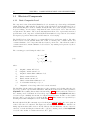
KP =
KI =
0.4881 − 0.4999 cos(3.964V ) + 0.1389 sin(3.964V ) V < 0.7
1
V > 0.7
(3.2)
2.657V 0.769 exp (−1.502V 1.769 ) V < 0.5
1
V > 0.5
(3.3)
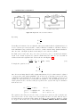
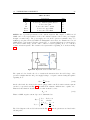
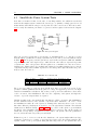
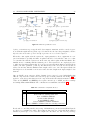
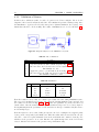
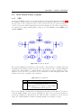
The model developed in Modelica for a composite load adopts the same strategy as the PSS/E
model, but includes also all the function related to the conversion and saturation. Therefore, the
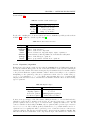
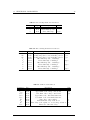
user is offered the possibility to configure the following parameters shown in Table 3.1:
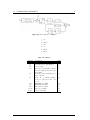
Table 3.1: Composite Load Parameters
Parameter
Sp
Si
Sy
a
b
P QBRAK
Type
Comp.
Comp.
Comp.
Comp.
Comp.
Real
Description
Original constant power load
Original constant current load
Original constant shunt admittance load
Coverting fraction for constant I load
Coverting fraction for constant Z load
Constant power characteristic threshold
Unit
p.u
p.u
p.u
p.u.
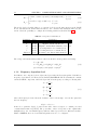
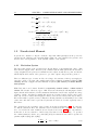
The voltage and current characteristics for the load should be then specified as following:
~ I~
P + jQ = V
P = KP <(SP ) + KI <(SI )V + <(SY )V 2
Q = KI =(SP ) + KI =(SI )V + =(SY )V
3.1.2
(3.4)
2
Frequency dependent load
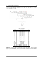
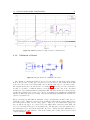
In addition to the composite load model presented previously, the Norwegian grid model includes a
frequency dependent model. The model used in PSS/E is LDFRAL. The model makes the constant
current and MVA components of all loads dependent on bus frequency according to following rules:
ω m
)
ωo
ω
Q = Qo ( )n
ωo
ω
Ip = Ipo ( )r
ωo
ω
Iq = Iqo ( )s
ωo
P = Po (
(3.5)
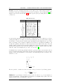
where the frequency is derived from the derivative of the load bus angle. wbase in the equation is
the base frequency.
˙ = wbase × ω
Angle
In the above equations, P, Q, Ip , Iq stand for the value of the load respect to constant power and
constant characteristic respectively. The power share of the load depends on the original value
multiplies the power of nominal frequency with user defined power factor for different load share.
Thus for LDFRAL, there are four additional parameter need to be configured.