Download EERA Manual - Civil Engineering

Department of Civil Engineering
EERA
A Computer Program for
Equivalent-linear Earthquake site Response Analyses
of Layered Soil Deposits
by
J. P. BARDET, K. ICHII, and C. H. LIN
August 2000
t
Table of Contents
1. INTRODUCTION ................................................................................................................1
2. EQUIVALENT LINEAR MODEL FOR SOIL RESPONSE .......................................................1
2.1 One-dimensional Stress-Strain Relationship ....................................................................1
2.2 Equivalent Linear Approximation of Nonlinear Stress-strain Response ..............................2
2.2.1 Model 1...................................................................................................................4
2.2.2 Model 2...................................................................................................................5
3. ONE-DIMENSIONAL GROUND RESPONSE ANALYSIS ......................................................6
3.1 Free surface, bedrock outcropping and rock outcropping motions .....................................9
3.2 Transient Motions ..........................................................................................................9
3.3 Iterative Approximation of Equivalent Linear Response .................................................. 10
4. DESCRIPTION OF EERA .................................................................................................. 11
4.1 System requirement, distribution files and download EERA ............................................ 11
4.2 Installing and removing EERA....................................................................................... 11
4.3 EERA commands ........................................................................................................ 12
4.4 EERA worksheets ........................................................................................................ 13
4.4.1 Earthquake data .................................................................................................... 14
4.4.2 Soil Profile............................................................................................................. 15
4.4.3 Material stress-strain damping-strain curves ............................................................ 19
4.4.4 Calculation ............................................................................................................ 19
4.4.5 Output (Acceleration) ............................................................................................. 20
4.4.6 Output (Strain)....................................................................................................... 21
4.4.7 Output (Ampli) ....................................................................................................... 21
4.4.8 Output (Fourier) ..................................................................................................... 22
4.4.9 Output (Spectra) .................................................................................................... 23
4.5 Running EERA ............................................................................................................ 23
4.6 Main features of EERA and comparison with SHAKE ..................................................... 24
4.7 Comparison of results from EERA and SHAKE .............................................................. 24
5. CONCLUSION.................................................................................................................. 24
6. REFERENCES ................................................................................................................. 25
7. APPENDIX A: SAMPLE PROBLEM ................................................................................... 26
7.1 Definition of problem .................................................................................................... 26
7.2 Results........................................................................................................................ 31
8. APPENDIX B: COMPARISON OF EERA AND SHAKE91 RESULTS ................................... 37
t
1. INTRODUCTION
During past earthquakes, the ground motions on soft soil sites were found to be generally larger
than those of nearby rock outcrops, depending on local soil conditions (e.g., Seed and Idriss,
1968). These amplifications of soil site responses were simulated using several computer
programs that assume simplified soil deposit conditions such as horizontal soil layers of infinite
extent. One of the first computer programs developed for this purpose was SHAKE (Schnabel et
al., 1972). More than 25 years after its release, SHAKE is still commonly used and referenced
computer programs in geotechnical earthquake engineering. SHAKE computes the response in a
horizontally layered soil-rock system subjected to transient and vertical travelling shear waves.
SHAKE is based on the wave propagation solutions of Kanai (1951), Roesset and Whitman
(1969), and Tsai and Housner (1970). SHAKE assumes that the cyclic soil behavior can be
simulated using an equivalent linear model, which is extensively described in the geotechnical
earthquake engineering literature (e.g., Idriss and Seed, 1968; Seed and Idriss, 1970; and
Kramer, 1996). SHAKE was modified many times (e.g., frequency-dependent equivalent strain;
Sugito, 1995). SHAKE91 is one of the most recent versions of SHAKE (Idriss and Sun, 1992).
In 1998, the computer program EERA was developed in FORTRAN 90 starting from the same
basic concepts as SHAKE. EERA stands for Equivalent-linear Earthquake Response Analysis.
EERA is a modern implementation of the well-known concepts of equivalent linear earthquake
site response analysis. EERA's implementation takes full advantages of the dynamic array
dimensioning and matrix operations in FORTRAN 90. EERA's input and output are fully
integrated with the spreadsheet program Excel.
Following the introduction, the second section of this report reviews the theory of equivalent linear
soil model, and one-dimensional ground response analysis. The two appendices contain a
sample problem and comparison between EERA and SKAKE91 results.
2. EQUIVALENT LINEAR MODEL FOR SOIL RESPONSE
2.1 One-dimensional Stress-Strain Relationship
The equivalent linear model represents the soil stress-strain response based on a Kelvin-Voigt
model as illustrated in Fig. 1. The shear stress τ depends on the shear strain γ and its rate γ& as
follows:
τ = G γ + ηγ&
(1)
where G is shear modulus and η the viscosity. In a one-dimensional shear beam column, the
shear strain and its rate are defined from the horizontal displacement u(z,t) at depth z and time t
as follows:
γ=
∂u ( z, t )
∂γ ( z , t ) ∂ 2 u ( z , t )
and γ& =
=
∂z
∂t
∂z∂t
γγ
(2)
τ
Gγ
G
η
ηγ
Figure 1. Schematic representation of stress-strain model used in equivalent-linear model.
1
In the case of harmonic motion, the displacement, strain and strain rate are:
u( z, t ) = U ( z ) e iω t , γ ( z, t ) =
dU i ωt
e = Γ( z ) ei ωt and γ& ( z, t ) = i ωγ ( z, t )
dz
(3)
where U(z) and Γ(z) are the amplitude of displacement and shear strain, respectively. Using Eq.
3, the stress-strain relation (i.e., Eq. 1) becomes in the case of harmonic loadings:
τ( z, t ) = Σ( z )e i ωt = (G + i ωη)
dU i ωt
dU iω t
e = G*
e = G*γ ( z, t )
dz
dz
(4)
*
where G is the complex shear modulus and Σ(z) is the amplitude of shear stress. After
*
introducing the critical damping ratio ξ so that ξ = ωη/2G , the complex shear modulus G
becomes:
G * = G + iωη = G(1 + 2iξ)
(5)
The energy dissipated W d during a complete loading cycle is equal to the area generated by the
stress-strain loop, i.e.:
Wd = ∫τ dγ
(6)
τc
In the case of strain-controlled harmonic loading of amplitude γc (i.e.,
γ (t ) = γ ce i ωt ), Eq. 6
becomes:
Wd = ∫
t + 2π ω
t
dγ
Re[τ( t ) ]Re   dt
 dt 
(7)
where only the real parts of the stress and strain rate are considered (Meirovitch, 1967). Using
Eq. 4, the real parts of stress and strain rate are:
dγ
Re [τ( t ) ] = γ c (G cos ωt − ωηsin ωt ) and Re   = −γ cωsin ωt
 dt 
(8)
Finally, Eq. 7 becomes:
t + 2π
1
Wd = ωγ c2 ∫
t
2
ω
[− G sin 2ωt + ωη(1 − cos 2ωt) ]dt = πωηγ c2
(9)
The maximum strain energy stored in the system is:
1
1
Ws = τcγ c = Gγ c2
2
2
The critical damping ratio
ξ=
Wd
4πWs
(10)
ξ can be expressed in terms of W d and W s as follows:
(11)
2.2 Equivalent Linear Approximation of Nonlinear Stress-strain Response
The equivalent linear approach consists of modifying the Kelvin-Voigt model to account for some
types of soil nonlinearities. The nonlinear and hysteretic stress-strain behavior of soils is
approximated during cyclic loadings as shown in Fig. 2. The equivalent linear shear modulus, G,
2
is taken as the secant shear modulus Gs , which depends on the shear strain amplitude γ. As
shown in Fig. 2a, Gs at the ends of symmetric strain-controlled cycles is:
Gs =
τc
γc
(12)
Stress ( τ)
where τc and γc are the shear stress and strain amplitudes, respectively. The equivalent linear
damping ratio, ξ, is the damping ratio that produces the same energy loss in a single cycle as the
hysteresis stress-strain loop of the irreversible soil behavior. Examples of data for equivalent
linear model can be found in Hardin and Drnevitch (1970), Kramer (1996), Seed and Idriss
(1970), Seed et al. (1986), Sun et al. (1988), and Vucetic and Dobry (1991).
Gmax
G sec
1
γc
Strain (γ )
G sec , ξ
τc
G sec
ξ
Shear strain (log scale)
(a)
(b)
Figure 2. Equivalent-linear model: (a) Hysteresis stress-strain curve; and (b) Variation of secant
shear modulus and damping ratio with shear strain amplitude.
In site response analysis, the material behavior is generally specified as shown in Fig. 2b. The
Gs -γ curves cannot have arbitrary shapes as they derive from τ−γ stress-strain curves. For
instance, the exclusion of strain-softening from the τ−γ curves imposes some restrictions on the
corresponding Gs -γ curves. Strain softening is a real physical phenomen which corresponds to a
decrease in stress with strain. Its inclusion requires complicated numerical techniques that are
beyond the scope of most enginering site responses. Without these special techniques, strainsoftening has been shown to create ill-posed boundary value problems, and undesirable
numerical effects such as numerical solutions that dependent strongly on spatial discretization
(i.e., mesh geometry). The exclusion of strain-softening implies that:
dτ
dGs
= Gs (γ ) +
γ ≥0
dγ
dγ
(13)
In the case of Gs -γ curves specified with discrete points (Gi, γi), Eq. 13 becomes:
∆G s
G (γ ) ∆γ
≥− s
Gmax
Gmax γ
(14)
where ∆Gs is the decrease in Gs corresponding to the increase ∆γ in γ, and Gmax is the maximum
value of Gs . Eq. 14 is equivalent to:
Gi +1 Gi ≥ 2 − γ i +1 γ i
(15)
3
max
1
Shear stress τ/τ max and G/G
Shear stress τ/τ max and G/G
max
Figure 3 illustrates a particular case of strain-softening, which is clearly visible on a stress-strain
response but difficult to detect from a Gs -γ curve.
0.8
0.6
Stress-strain
0.4
G/Gmax
0.2
0
0
0.05
0.1
0.15
0.2
0.25
Shear strain γ
1
0.8
Softening
0.6
0.4
Stressstrain
0.2
G/Gmax
0
0.001
0.01
0.1
1
Shear strain γ
Figure 3. An example of strain softening in τ/τmax and G/Gmax curves plotted in linear and semilogarithmic scales.
As shown in Fig. 2b, the equivalent linear model specifies the variation of shear modulus and
damping ratio with shear strain amplitude. Additional assumptions are required to specify the
effects of frequency on stress-strain relations. For this purpose, two basic models have been
proposed.
2.2.1 Model 1
Model 1 is used in the original version of SHAKE (Schnabel et al., 1972). It assumes that ξ is
*
constant and independent of ω, which implies that the complex modulus G is also independent of
ω. The dissipated energy during a loading cycle is:
Wd = 4πWsξ = 2π ξ Gγ c2 = πηγc2ω
(16)
The dissipated energy increases linearly with ξ, and is independent of ω, which implies that the
area of stress-strain loops is frequency independent. The amplitudes of complex and real shear
modulus are related through:
G* = G 1 + 4ξ 2
(17)
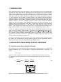
which implies that |G | increases with ξ. Figure 4 shows the variation of |G |/G with ξ. The
amplitude of the complex shear modulus can vary as much as 12 % when ξ reaches 25%.
*
*
4
2.5
|G*|/G
2
1.5
1
0
0.2
0.4
0.6
0.8
1
Critical Damping Ratio ξ
Figure 4. Normalized variation of complex shear modulus amplitude with critical damping ratio
(Model 1).
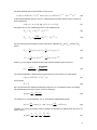
2.2.2 Model 2
Model 2 is used in SHAKE 91 (Idriss and Sun, 1992). It assumes that the complex shear modulus
is a function of ξ:
{
G* = G (1 − 2ξ2 ) + 2ξi 1 − ξ 2
}
(18)
The assumption above is a constitutive assumption that pertains to the description of material
behavior. It implies that the complex and real modulus have the same amplitude, i.e.:
G* = G{(1 − 2ξ2 ) 2 + 4ξ 2 (1 − ξ2 )} = G
(19)
The energy dissipated during a loading cycle is:
t + 2π ω
1
Wd = ωγ c2 ∫
2Gξ 1 − ξ 2 dt = 2π Gξ 1 − ξ2 γ c2
t
2
(20)
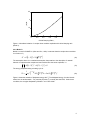
Figure 5 shows the variation of dissipated energy with ξ. The dissipated energy of model 2 tends
toward zero as tends toward 1. For practical purposes, ξ is usually less than 25%. Under these
conditions, the energies dissipated by Models 1 and 2 are similar.
5
1
0.8
Model 2
Dissipated Energy W
d /(2
G
c
2
)
Model 1
0.6
0.4
0.2
0
0
0.2
0.4
0.6
0.8
1
Critical Damping Ratio ξ
Figure 5. Normalized variation of energy dissipated per loading cycle as a function of critical
damping ratio for models 1 and 2.
3. ONE-DIMENSIONAL GROUND RESPONSE ANALYSIS
Figure 6 schematizes the assumptions of one-dimensional equivalent linear site response
analysis. As shown in Fig. 6, a vertical harmonic shear wave propagates in a one-dimensional
layered system. The one-dimensional equation of motion for vertically propagating shear waves
is:
ρ
∂ 2 u ∂τ
=
∂t 2 ∂z
(21)
where ρ is the unit mass in any layer. Assuming that the soil in all layers behaves as a KelvinVoigt solid (i.e., Eq. 1), Eq. 22 becomes:
ρ
∂2 u
∂2 u
∂ 3u
=
G
+
η
∂t 2
∂z 2
∂z 2 ∂t
(22)
6
Layer
Coordinate
u1
1
z1
2
•
•
Properties
G 1 ξ1 ρ1
•
•
•
um
zm
G m ξm ρm
m+2
•
•
Gm+1 ξm+1 ρm+1
h m+1
u m+2
•
•
•
zm+2
uN
N
hm
u m+1
m+1
zm+1
h1
u2
z2
m
Thickness
zN
G N ξN ρN
h N= ∞
Figure 6. One-dimensional layered soil deposit system (after Schnabel et al., 1972).
For harmonic waves, the displacement can be written as:
u( z, t ) = U ( z ) e iω t
(23)
Using Eq. 23, Eq. 22 becomes:
d 2U
( G + iωη) 2 = ρω 2U
dz
(24)
and admits the following general solution:
U ( x) = Ee ik* z + Fe −ik * z
(25)
ρω 2
ρω 2
where k =
=
is the complex wave number. After introducing the critical damping
G + iωη G *
*
ratio ξ so that ξ = ωη/2G , the complex shear modulus G becomes:
*2
G * = G + iωη = G(1 + 2iξ)
(26)
The solution of Eq. 24 is:
u ( z , t ) = ( Eeik * z + Fe − ik* z )e i ωt
(27)
and the corresponding stress is:
τ( z , t ) = ik * G* ( Eeik * z − Fe − ik *z )e i ωt
(28)
The displacements at the top (z = 0) and bottom ( z = hm) of layer m of thickness hm are:
*
*
um (0, t ) = um = ( Em + Fm )ei ω t and u m ( hm , t ) = ( E m e ikmh m + Fm e −ik mhm )e i ωt
(29)
7
The shear stresses at the top and bottom of layer m are:
*
*
τm ( 0, t ) = ik m* Gm* ( E m − Fm )e i ω t and τm ( hm , t ) = ik *m Gm* ( Em e ikm hm − Fm e −ik mhm )e i ωt
(30)
At the interface between layers m and m+1, displacements and shear stress must be continuous,
which implies that:
u m ( hm , t ) = u m +1 ( 0, t ) and τm ( hm , t ) = τ m +1 ( 0, t )
(31)
Using Eqs. 29 to 31 the coefficients Em and Fm are related through:
E m +1 + Fm +1 = E m e ikmh m + Fm e − k mhm
*
Em +1 − Fm + 1 =
*
*
*
km* Gm*
( Em eik mh m − Fm e −ik mh m )
*
*
km + 1Gm +1
(32)
(33)
Eqs. 32 and 33 give the following recursion formulas for amplitudes Em+1 and Fm+1 in terms of Em
and Fm:
E m +1 =
1
*
1
*
E m (1 + α *m ) e ikmhm + Fm (1 − α *m ) e −ikm hm
2
2
Fm +1 =
where
*
*
1
1
E m (1 − α *m )e ik mhm + Fm (1 + α *m )e −ikmh m
2
2
(34)
(35)
αm* is the complex impedance ratio at the interface between layers m and m+1:
k m* G * m
α = *
=
k m +1 G * m + 1
*
m
ρm G * m
ρ m +1 G * m +1
(36)
The recursive algorithm is started at the top free surface, for which there is no shear stress:
τ1 ( 0, t ) = ik1* G1* ( E1 − F1 )e i ωt = 0
(37)
which implies:
E1 = F1
(38)
Eqs. 34 and 35 are then applied successively to layers 2 to m. The transfer function Amn relating
the displacements at the top of layers m and n is defined by
Amn (ω) =
The velocity
um Em + Fm
=
un
En + Fn
(39)
u& ( z , t ) and acceleration u&&( z , t ) are related to displacement through:
u& ( z , t ) =
∂u
∂ 2u
= iω u ( z , t ) and u&&( z , t ) = 2 = −ω2 u ( z , t )
∂t
∂t
(40)
Therefore Amn is also the transfer function relating the velocities and diplacements at the top of
layers m and n:
Amn (ω) =
um u& m u&&m Em + Fm
=
=
=
un u& n u&&n
En + Fn
(41)
8
The shear strain at depth z and time t can be derived from Eq. 25:
γ (z , t) =
∂u
= ik * ( Eeik * z − Fe − ik *z )e i ωt
∂z
(42)
The corresponding shear stress at depth z and time t is:
τ( z, t ) = G * γ ( z , t )
(43)
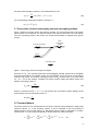
3.1 Free surface, bedrock outcropping and rock outcropping motions
Figure 7 defines four terms used in site response analysis. The free surface motion is the motion
at the surface of a soil deposit. The bedrock motion is the motion at the base of the soil deposit.
The rock outcropping motion is the motion at a location where bedrock is exposed at the ground
surface.
Rock
outcr oppi ng
motion
Free surface motion
2E N
2E 1
E N +FN
Bedrock motion
Incoming motion
EN
Figure 7. Terminology used in site response analysis.
As shown in Fig. 7, the incoming shear wave that propagates vertically upward has for amplitude
EN through the bedrock. The bedrock motion has for amplitude EN+FN at the top of the bedrock
under the soil layers. The bedrock outcropping motion is 2EN, because there is no shear stress
(i.e., EN = FN) on free surfaces. Therefore the transfer function relating the bedrock motion and
bedrock outcropping motion is:
ANN (ω) =
2EN
E N + FN
(44)
When it is assumed that E1 = F1 = 1 on free surface, then the transfer function relating the free
surface motion and rock outcropping motion is:
A1′N (ω) =
1
EN
(45)
3.2 Transient Motions
The theory above for the one-dimensional soil column response was presented for steady state
harmonic motions, i.e., in the frequency domain. It can be extended to the time histories of
transient motions using Fourier series (e.g., Bendat and Piersol, 1986). A real-valued or complexvalued function x (t) can be approximated by a discrete series of N values as follows:
N −1
N −1
N −1
k=0
k =0
k =0
xn = ∑ X k e iω k t n = ∑ X k e iω k n ∆ t = ∑ X k e 2 πikn / N n = 0, …, N-1
(46)
9
The values xn correspond to times tn = n ∆t where ∆t is the constant time interval (i.e., x(n∆t) = xn
for n = 0, …, N-1). The discrete frequencies ωk are:
ωk = 2π
k
N ∆t
k = 0, …, N-1
(47)
The Fourier components are:
Xm =
1
N
N −1
∑x e
n
−2 πikm / N
m = 0, …, N-1
(48)
k =0
The coefficients Xm are calculated by the Fast Fourier Transform algorithm, which was originally
developed by Cooley and Tukey (1965). The number of operations scales as N logN, which
justifies the name of Fast Fourier Transform (i.e., FFT).
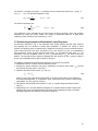
3.3 Iterative Approximation of Equivalent Linear Response
As previously described in Fig. 3, the equivalent linear model assumes that the shear modulus
and damping ratio are functions of shear strain amplitude. In SHAKE, the values of shear
modulus and damping ratio are determined by iterations so that they become consistent with the
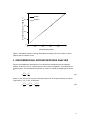
level of strain induced in each layer. As shown in Fig. 8, the values of G0 and ξ0 are initialized at
their small strain values, and the maximum shear strain γmax and effective shear strain γeff1 are
1
calculated. Then the compatible values G1 and ξ1 corresponding to γ eff are found for the next
iteration. The equivalent linear analysis is repeated with new values of G and ξ until the values of
G and ξ are compatible with the strain induced in all layers.
The iteration procedure for equivalent linear approach in each layer is as follows:
i
i
1. Initialize the values of G and ξ at their small strain values.
2. Compute the ground response, and get the amplitudes of maximum shear strain γmax from the
time histories of shear strain in each layer.
3. Determine the effective shear strain γeff from γmax :
γ ieff = Rγ γ imax
(49)
where Rγ is the ratio of the effective shear strain to maximum shear strain, which depends on
the earthquake magnitude. Rγ is specified in input; it accounts for the number of cycles during
earthquakes. Rγ is the same for all layers.
4. Calculate the new equivalent linear values Gi+1 and ξi+1 corresponding to the effective shear
strain γeff.
5. Repeat steps 2 to 4 until the differences between the computed values of shear modulus and
damping ratio in two successive iterations fall below some predetermined value in all layers.
Generally 8 iterations are sufficient to achieve convergence.
10
Shear modulus
G0
G1
Damping ratio
G2
ξ2
ξ1
ξ0
γ 1eff γ2 eff
Shear strain amplitude (logarithmic scale)
Figure 8. Iteration of shear modulus and damping ratio with shear strain in equivalent linear
analysis.
4. DESCRIPTION OF EERA
EERA (Equivalent-linear Earthquake site Response Analysis) is a modern implementation of the
equivalent-linear concept of earthquake site response analysis, which was previously
implemented in the original and subsequent versions of SHAKE (Schnabel et al., 1972; and Idriss
and Sun, 1991).
4.1 System requirement, distribution files and download EERA
EERA requires Windows 95/98/NT and EXCEL 97 or later. EERA does not work for other
operating systems and spreadsheet program. All the files required for EERA can be downloaded
from http://geoinfo.usc.edu/gees in one zip file named EERA.zip, which contains the following
files:
• EERA.xla (389 kB), Microsoft Excel Add-in
• EERAM.xls (4627 kB), Example Startup file (metric units)
• EERA.xls (3988kB), Example Startup file (British units)
• EERA.dll (97kB), EERA Dynamic Link Library
• Diam.acc (21kB), Example earthquake input acceleration file
4.2 Installing and removing EERA
It is recommended to install EERA on your computer system as follows:
1. Copy the distribution files in a new directory on your hard drive
2. Move EERA.dll and EERA.xla in the same directory of your choice. This is a critical step
as these files cannot be moved easily later.
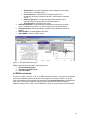
3. In EXCEL, install the Add-in EERA.xla using Tools and Add-ins... As shown in Fig. 9,
use Browse to locate EERA.xla. Do not move EERA.xla after installing it.
11
4.
When EERA is properly installed, the EERA menu will appear to the right of the EXCEL
pull-down menus (Fig. 10).
EERA can be de-installed by using Remove EERA in the EERA pull-down menu.
Figure 9. The EXCEL Add-ins menu.
Location of EERA pull down menu
Figure 10. After a successful installation of EERA, the pull-down menu EERA should appear to
the right of EXCEL pull down menus.
4.3 EERA commands
As shown in Fig. 11, there are seven commands in the EERA pull-down menu
1. Process Earthquake Data - Read and process earthquake input motion (input/output in
worksheet Earthquake)
2. Calculate Compatible Strain - Read profile, material curves, and execute the main
iterative calculation (input/output in worksheet Iteration)
3. Calculate Output
• Acceleration/Velocity/Displacement - Calculate time history of
acceleration, relative velocity and displacement at the top of selected
sub-layers (input/output in worksheet Acceleration ...)
• Stress/Strain - Calculate stress and strain at the middle of selected sublayers (input/output in worksheets Strain ...)
12
•
4.
5.
6.
7.
Amplification - Calculate amplification factors between two sub-layers
(input/output in worksheets Ampli ...)
• Fourier Spectrum - Calculate Fourier amplitude spectrum of
acceleration at the top of selected sub-layer. (input/output in worksheet
Fourier ...)
• Response Spectrum - Calculate all response spectra at the top of
selected sub-layers (input/output in worksheet Spectra ...)
• All of the above - Calculate all the output
Duplicate Worksheet - Duplicate selected worksheet for defining new material
curves, and adding new output (e.g., response spectra for several sub-layers)
Delete Worksheet - Delete unnecessary worksheet (some worksheet cannot be
deleted)
Remove EERA - De-install EERA from EXCEL
About EERA - Number of EERA version
Figure 11. The EERA pull-down menu.
EERA
1.
2.
3.
commands are to be used in the following order:
Process Earthquake Data
Calculate Compatible Strain
Calculate Output
4.4 EERA worksheets
As shown in Table 1 and Figs. 12 to 19, an EERA workbook is made of nine types of worksheets,
which have predefined names that should not be changed. As indicated in Table 1, six of nine
types of worksheet can be duplicated and modified using Duplicate Worksheet in the EERA pulldown menu. This feature is useful for obtaining output at several sub-layers and defining
additional material curves. Table 1 also indicates the number of input required in each worksheet.
13
Table 1. Types of worksheets in EERA and their contents
Worksheet
Earthquake
Mat I
Contents
Earthquake input time history
Material curves (G/Gmax and Damping
versus strain for material type i
Profile
Vertical profile of layers
Iteration
Results of main calculation
Time history of
acceleration/velocity/displacement
Time history of stress and strain
Amplification between two sub-layers
Fourier amplitude spectrum of
acceleration
Response spectra
Acceleration
Strain
Ampli
Fourier
Spectra
Duplication
Number of input
No
7
Yes
Dependent on number of
soil layers
No
Dependent on number of
data points per material
curve
No
3
Yes
2
Yes
Yes
Yes
1
4
Yes
3
3
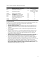
4.4.1 Earthquake data
As shown in Fig. 12, Worksheet Earthquake is used to define the earthquake input motion. There
are six required entries and one optional entry. All entries are in blue characters.
• Cell A1: the earthquake name is optional.
• Cell B2: the time step ∆T is the time interval between the evenly spaced data points of the
time history of input ground motion.
• Cell B3: the desired maximum frequency is used to scale the peak amplitude of the input
acceleration.
• Cell B4: the maximum frequency cut-off fmax is used to filter the high frequencies from the
input acceleration.
• Cell B5: the frequency cut-off fmax can be used to eliminate high frequencies from the input
acceleration records. All the calculations will be performed for frequencies between 0 and
fmax. This option is useful to overcome the overflow calculation errors in Eq. 34 that are
usually caused for very high frequencies.
• Cell B6: the number m of data points in the FFT calculation can be defined. m is generally
selected to be larger than the number n of data points in the input acceleration time history. In
this case the input record is padded with zero in order to produce a record of length n.
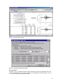
• Cell B7: The input acceleration can be read from an external data file. EERA is capable of
reading many earthquake data formats from external data files. In this case, select Yes in
Cell B5, then follow EERA instructions for selecting data format. As shown in Fig. 13, you can
open earthquake files of different types, eliminate headers, and select various formats.
Header lines are skipped by selecting a starting row number in Fig. 13. If you do not wish to
import earthquake data for an external file, you may select No in Cell B5. This option is useful
when (1) you have already imported earthquake data, or (2) you have pasted your own
earthquake acceleration time history in column B15-.
14
Figure 12. Worksheet Earthquake.
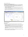
Figure 13. Importing earthquake input data.
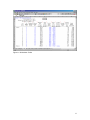
4.4.2 Soil Profile
As shown in Fig. 14, Worksheet Profile is used to define the geometry and properties of the soil
profile. All input data are in blue cells. Input data can be graphically checked as shown in Fig. 15.
• Cell A1: the soil profile is optionally named.
15
•
•
•
•
•
•
•
•
•
•
Column C6- : the number of material type is specified for each layer. Each material type i is
defined in a separate worksheet called Mat i.
Column D6- : each layer may be subdivided in several sub-layers. This feature improves the
accuracy of calculations.
Column E6- : the thickness of each layer is specified.
Column F6- : The small strain values of shear modulus is entered in the unit specified in Cell
F5. If this column is left blank then the shear wave velocity must be input in column I6Column G6- : The initial value of critical damping is only required when the material number
on this row is equal to zero, (i.e., no material curve is defined).
Column H6- : The total unit weight is entered in the physical unit specified in Cell H5
Column I6- : The shear wave velocity is enter in the physical unit specified in Cell I5. If this
column is left blank then the maximum shear modulus must be input in column F6Column J6- : The location and type of earthquake motion is defined by specifying only once in
this column either Outcrop for an outcropping rock motion, or Inside for a non outcropping
motion.
Column K6- : The depth of the water table can be specified in order to calculate vertical
effective stresses. This input is optional as it is only used in the calculation of initial stresses,
and not in other calculations.
Cell E3: The average shear wave velocity V of the soil profile is calculated as follows:
V =
N
∑h v
1
N
∑h
i i
i =1
i
i =1
where hi is the height of layer i, vi is the shear wave velocity in layer i, and N is the total
number of layers.
•
Cell E2: The fundamental period T of the soil profile is calculated as T = 4 H/V where H is the
total thickness of soil profile and V is the average shear wave velocity of soil profile as
calculated in Cell E2.
Note:
The average shear wave velocity V and fundamental period T can also be computed as follows
N
V=
∑h
i
i =1
N
hi
∑v
i =1
N
and
T = 4∑
i =1
hi
vi
i
16
Figure 14. Worksheet Profile.
17
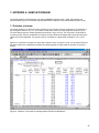
18
Figure 15. Worksheet Profile.
4.4.3 Material stress-strain damping-strain curves
As shown in Fig. 16, several material stress-strain and damping-strain curves can be defined.
You may generate additional worksheets for material properties by using Duplicate worksheet
from the main EERA menu. Input data can be graphically checked as shown in Fig. 16.
• Cell A1: the material type is optionally named.
• Column A3- : the values of shear strain corresponding to ratio G/Gmax data in column B3- are
entered as increasing numbers.
• Column B3- : Enter the values of ratio G/Gmax corresponding to strain data in column A3-.
• Column C3- : the values of shear strain corresponding to critical damping ratio data in column
D3- are entered as increasing numbers.
• Column D3- : Enter the values of critical damping ratio corresponding to strain data in column
C3-.
Figure 16. Worksheet Mat.
4.4.4 Calculation
As shown in Fig. 17, the worksheet iteration has three entries (shown in blue characters):
• Cell E1: the number of iterations is specified. Eight iterations are usually enough to achieve a
satisfactory convergence.
• Column E2: The ratio of equivalent uniform strain is entered. The ratio of equivalent uniform
strain accounts for the effects of earthquake duration. Typically this ratio ranges from 0.4 to
0.75 depending on the input motion and which magnitude earthquake it is intended to
represent. The following equation may be used to estimate this ratio (Idriss and Sun, 1992):
ratio = (M - I)/10
in which M is the magnitude of the earthquake. For example, for M = 5, the ratio would be
0.4.
• Column E3: the type of linear equivalent model is selected. There are two options: (1) model
of the original SHAKE, and (2) model of SHAKE91.
19
Figure 17. Worksheet Iteration.
4.4.5 Output (Acceleration)
As shown in Fig. 18, the worksheet Acceleration defines the time history of acceleration/ relative
velocity and relative displacement at a selected sublayer. The worksheet can be duplicated by
using Duplicate Worksheet in the EERA menu.
• Cell D1: The number of selected sublayer is specified.
• Cell D2: The type of selected sublayer is specified. The type can be either outcropping or not
outcropping.
•
Figure 18. Worksheet Acceleration.
20
4.4.6 Output (Strain)
As shown in Fig. 19, the worksheet Strain defines the time history of stress, strain and dissipated
energy, and stress-strain loops. The worksheet can be duplicated by using Duplicate Worksheet
in the EERA menu.
• Cell D1: The number of selected sublayer is specified.
•
Figure 19. Worksheet Strain.
4.4.7 Output (Ampli)
As shown in Fig. 20, the worksheet Ampli defines the amplification factor between two sublayers.
The worksheet can be duplicated by using Duplicate Worksheet in the EERA menu.
• Cell D1: The number of the first sublayer is specified.
• Cell D2: The type of the first sublayer is specified. It can be either outcropping or not
outcropping.
• Cell D3: The number of the second sublayer is specified.
• Cell D4: The type of the second sublayer is specified. It can be either outcropping or not
outcropping.
•
21
Figure 20. Worksheet Ampli.
4.4.8 Output (Fourier)
As shown in Fig. 21, the worksheet Fourier defines the Fourier spectrum for a selected sublayer.
The worksheet can be duplicated by using Duplicate Worksheet in the EERA menu.
• Cell D1: The number of the selected sublayer is specified.
• Cell D2: The type of the first sublayer is specified. It can be either outcropping or not
outcropping.
• Cell D3: The number of moving averages is specified. This feature filtered noises in the
Fourier spectrum.
•
Figure 21. Worksheet Fourier.
22
4.4.9 Output (Spectra)
As shown in Fig. 22, the worksheet Spectra defines response spectra for a selected sublayer.
The worksheet can be duplicated by using Duplicate Worksheet in the EERA menu.
• Cell D1: The number of the selected sublayer is specified.
• Cell D2: The type of the first sublayer is specified. It can be either outcropping or not
outcropping.
• Cell D3: The selected value of critical damping ratio for the response spectra.
Figure 21. Worksheet Spectra.
4.5 Running EERA
EERA is distributed with the example file EERAM.xls. Once you have opened this example file
from within EXCEL, you can perform the following operations using the EERA pull-down menu:
1. Process Earthquake Data
2. Calculate Compatible Strain
3. Calculate Output and All of the Above
As you perform these steps above, the output data will be first erased and then recalculated. No
user-input in the worksheet is required in this example. Some of the output figures are displayed
in Appendix A.
You may attempt to define your own problem. EERA input data is in the cells with blue
characters. A help message is displayed as you move the cursor to input cells. A suggested way
to proceed is as follows:
1. Copy EERAM.xls (or an existing EERA file), and rename it as you like (e.g.
Myrun.xls)
2. In Myrun.xls, retype on existing blue cells to enter your data. You may use additional
line in worksheets Mat..., Profile and Earthquake
3. If additional material curves or output is required, duplicate worksheets using
Duplicate Worksheet
4. Run EERA by using successively
1. Process Earthquake Data
2. Calculate Compatible Strain
3. Calculate Output and All of the Above
23
In general, a EERA site response analysis is performed in three successive steps.
Step 1
• Define all earthquake data in worksheet Earthquake
• Use Process Earthquake Data
Step 2
• Define the soil profile in worksheet Profile
• Define all the material stress-strain response curves in worksheets Mat...
• Define the main calculation parameters in worksheet Iteration
• Use Calculate Compatible Strain
Step 3
• Define the input parameters in worksheets Acceleration
• Use Calculate Output and Acceleration/...
• Define the input parameters in worksheets Strain
• Use Calculate Output and Stress-Strain
• Repeat the same process for Ampli, Fourier, and Spectra
4.6 Main features of EERA and comparison with SHAKE
EERA and SHAKE91 are based on the same fundamental principles. However their
implementations are substantially different. The main differences are:
• EERA dynamic library is implemented in FORTRAN 90. All matrix and vector calculations are
performed without indices. One of the main advantages of FORTRAN 90 over its
predecessors is the dynamic dimensioning of arrays. The size of the arrays adapt to the size
of the problems, within the limit of the computer available memory. EERA dimensions
internally its work arrays depending on the problem size.
• As a benefit of dynamic dimensioning, there is no limit on the total number of material
properties and soil layers in EERA. The sublayers and soil properties are no longer limited to
50 and 13, respectively, as in SHAKE91.
• As another benefit of dynamic dimensioning, the users can prescribe the number of data
points for FFT beyond 4096. Larger numbers of data points are useful to describe high
frequencies in the calculations. However, longer computation times are likely to result from
larger number of data points in the FFT calculations.
• The relative displacement and velocity can be calculated in sublayers, in the same way as
acceleration.
• The users can select calculations for a filtered or unfiltered object motion. SHAKE91 uses an
optional low-pass filter, which eliminates the high frequency response. The high frequency
components may be useful for the users interested in dynamic response of structures with
high frequency components (e.g., structural equipment).
• EERA uses an optimized version (IMSL, 1998) of the Cooley and Tukey algorithm for FFT.
4.7 Comparison of results from EERA and SHAKE
The results of EERA and SHAKE91 were found to be identical in the example provided with
SHAKE91. This comparison is detailed in Appendix B.
5. CONCLUSION
EERA is a modern implementation of the equivalent linear concept for earthquake site response
analysis, which was previously implemented in SHAKE. EERA is fully integrated with a
spreadsheet program EXCEL and gives many new additional features to users, such as unlimited
number of soil properties and soil layers, and user-defined number of data points for fast Fourier
transform.
24
6. REFERENCES
1.
2.
3.
4.
5.
6.
7.
8.
9.
10.
11.
12.
13.
14.
15.
16.
17.
18.
19.
20.
21.
Bendat, J. S., and A. G. Piersol, (1986) Random Data, Analysis and Measurement
Procedures, John Wiley & Sons, New York, pp. 334-383.
Cooley, J. W. and Tukey, J. W. (1965) "An Algorithm for the Machine Calculations of
Complex Fourier Series," Mathematics of Computation, Vol. 19, No. 90, pp. 297-301.
Hardin, B. O. and Drnevich, V. P. (1972) "Shear Modulus and Damping in Soils: I.
Measurement and Parameter Effects, " Journal of Soil Mechanics and Foundation Division,
ASCE, Vol. 98, No. 6, pp. 603-624.
Hardin, B. O. and Drnevich, V. P. (1972) "Shear Modulus and Damping in Soils: II. Design
Equations and Curves," Journal of Soil Mechanics and Foundation Division, ASCE, Vol. 98,
No. 7, pp. 667-691.
Idriss, I. M. (1990) "Response of Soft Soil Sites during Earthquakes", Proceedings, Memorial
Symposium to honor Professor Harry Bolton Seed, Berkeley, California, Vol. II, May.
Idriss, I. M. and Seed, H. B. (1968) "Seismic Response of Horizontal Soil Layers," Journal of
the Soil Mechanics and Foundations Division, ASCE, Vol. 94, No. 4, pp.1003-1031.
Idriss, I. M. and Sun, J. I. (1992) “User’s Manual for SHAKE91,” Center for Geotechnical
Modeling, Department of Civil Engineering, University of California, Davis.
IMSL (1998). Math Library, Chapter 6: Transforms, documentation available from Visual
Numerics, Houston, Texas, at http://www.vni.com/products/imsl/MATH.pdf, pp. 772-777.
Kanai, K. (1951) "Relation Between the Nature of Surface Layer and the Amplitude of
Earthquake Motions," Bulletin, Tokyo Earthquake Research Institute.
Kramer, S. L. (1996). Geotechnical Earthquake Engineering, Prentice Hall, Upper Saddle
River, New Jersey, pp. 254-280.
Lysmer, J., Seed, H. B. and Schnabel, P. B. (1971) "Influence of Base–Rock
Characteristics on Ground Response," Bulletin of the Seismological Society of America, Vol.
61, No. 5, pp. 1213-1232.
Matthiesen, R. B., Duke, C. M., Leeds, D. J. and Fraser, J. C. (1964) "Site Characteristics
of Southern California Strong-Motion Earthquake Stations, Part Two," Report No. 64-15.
Department of Engineering, University of California, Los Angeles. August.
Meirovitch, L., (1967) "Analytical Methods in Vibrations," The MacMillan Company, NY, pp.
400-401.
Roesset, J. M. and Whitman, R. V. (1969) "Theoretical Background for Amplification
Studies," Research Report No. R69-15, Soils Publications No. 231, Massachusetts Institute
of Technology, Cambridge.
Schnabel, P. B., Lysmer, J., and Seed, H. B. (1972) “ SHAKE: A Computer Program for
Earthquake Response Analysis of Horizontally Layered Sites”, Report No. UCB/EERC-72/12,
Earthquake Engineering Research Center, University of California, Berkeley, December,
102p.
Seed, H. B. and Idriss, I. M. (1970) "Soil Moduli and Damping Factors for Dynamic
Response Analysis", Report No. UCB/EERC-70/10, Earthquake Engineering Research
Center, University of California, Berkeley, December, 48p.
Seed, H. B., Wong, R. T., Idriss, I. M. and Tokimatsu, K. (1986) "Moduli and Damping
factors for Dynamic Analyses of Cohesionless Soils," Journal of the Geotechnical
Engineering Division, ASCE, Vol. 11 2, No. GTI 1, November, pp.1016-1032.
Sugito, M. (1995) “Frequency-dependent equivalent strain for equi-linearized technique,”
Proceedings of the First International Conference on Earthquake Geotechnical Engineering,
Vol. 1, A. A. Balkena, Rotterdam, the Netherlands, pp. 655-660.
Sun, J. I., Golesorkhi, R. and Seed, H. B. (1988) "Dynamic Moduli and Damping Ratios for
Cohesive Soils," Report No. UCB/EERC-88/15, Earthquake Engineering Research Center,
University of California, Berkeley, 42p.
Tsai, N. C., and G. W. Housner, 1970, “Calculation of Surface Motions of a Layered Half
Space,” Bulletin of the Seismological Society of America, Vol. 60, No. 5, pp. 1625-1651.
Vucetic, M. and Dobry, R. (1991) "Effect of Soil Plasticity on Cyclic Response," Journal of
the Geotechnical Engineering Division, ASCE, Vol. 111, No. 1, January, pp. 89-107.
25
7. APPENDIX A: SAMPLE PROBLEM
The sample problem is identical to the one used for SHAKE91 (Idriss and Sun, 1992). Input data for this
sample problem is given in the EXCEL spreadsheets EERA.xls (British units) and EERAM.xls (Metric units).
7.1 Definition of problem
The sample problem is a 150-ft soil profile consisting of clay and sand overlying a half-space. The geometry of
the soil layers is defined in Fig. A1. The profiles of shear wave velocity and unit weight are shown in Fig. A2.
The three different types of material properties are defined in Figs. A3 to A5. The input motion is specified as
an outcrop motion from the acceleration time history recorded at Diamond Heights (EW component) during the
1989 Loma Prieta earthquake. The ground motion is normalized to a target peak acceleration of 0.1 g (Fig.
A6).
Figures A1 to A6 shows a snapshot of the actual computer screen. As shown in Figs. A7 and A8 and Table A1,
the same results can be displayed and pasted as individual graphs or tables ready for inclusion in technical
reports.
Figure A1. Definition of soil profile in example problem (EXCEL file EERAM.xls).
26
Figure A2. Profiles of shear wave velocity and unit weight of sample problem (EXCEL file EERAM.xls).
Figure A3. Material properties of material type No.1 (EXCEL file EERAM.xls).
27
Figure A4. Material properties of material type No.2 (EXCEL file EERAM.xls).
Figure A5. Material properties of material type No.3 (EXCEL file EERAM.xls).
28
Figure A6. Time history of input ground motion (EXCEL file EERAM.xls).
1
30
G/G max
20
0.6
Shear Modulus
15
Damping Ratio
0.4
10
0.2
0
0.0001
Damping Ratio (%)
25
0.8
5
0
0.001
0.01
0.1
1
10
Shear Strain (%)
Figure A7. Modulus reduction and damping ratio curves used for sample problem (material No. 1).
29
Table A1. Values of modulus reduction and damping ratio curves used for sample problem.
Modulus for clay (Seed and Sun, 1989) upper range and damping for clay (Idriss 1990)
G/Gmax
Strain (%)
0.0001
0.0003
0.001
0.003
0.01
0.03
0.1
0.3
1
3
10
1
1
1
0.981
0.941
0.847
0.656
0.438
0.238
0.144
0.11
Strain (%)
0.0001
0.0003
0.001
0.003
0.01
0.03
0.1
0.3
1
3.16
10
Damping (%)
0.24
0.42
0.8
1.4
2.8
5.1
9.8
15.5
21
25
28
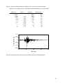
Acceleration (g)
0.1
0.05
0
-0.05
-0.1
-0.15
0
10
20
30
40
Time (sec)
Figure A8. Acceleration time history for Diamond Heights during Loma Prieta earthquake.
30
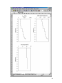
7.2 Results
The results of the site response analysis are contained in the EXCEL spreadsheets EERA.xls and
EERAM.xls. Some of these results are shown in Figs. A9 to A15.
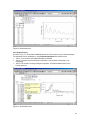
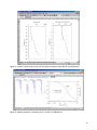
Figure A9 shows the variation with depth of maximum shear strain, ratio G/Gmax and damping ratio at
each of the calculation iteration step. At the first calculation step, the ratio G/Gmax is equal to 1, and the
damping ratio is constant. After a few calculation steps, the distributions of ratio G/Gmax and damping ratio
converge toward their final values. Figure A10 shows the corresponding variation with depth of maximum
shear stress during calculations, and the converged maximum acceleration.
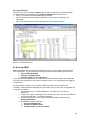
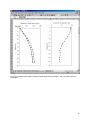
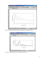
Figure A11 shows the computed time histories of acceleration, relative velocity and relative displacement
at the free surface. The relative displacement and velocity are evaluated relative to the bottom of the soil
profile. Figure A12 shows the time histories of shear strain, shear stress and energy dissipated per unit
volume, and the stress-strain loop computer at sublayer No. 4
Figure A13 shows the computed amplitude of amplification ratio between bottom and free surface. Figure
A14 shows the computed amplitude of Fourier amplitude at free surface. Finally, Fig. A15 displays the
acceleration response spectrum computed at free surface for a 5% critical damping ratio.
Figure A9. Variation with depth of maximum shear strain, ratio G/Gmax and damping ratio.
31
Figure A10. Variation with depth of maximum shear stress during calculation, and converged maximum
acceleration.
32
Figure A11. Computed time histories of acceleration, relative velocity and relative displacement at the
free surface.
33
Figure A12. Computed time histories of shear strain, shear stress and energy dissipated per unit volume,
and stress-strain loop at sublayer No. 4.
34
Figure A13. Computed amplitude of amplification ratio between bottom and free surface.
Figure A14. Computed amplitude of Fourier amplitude at free surface.
35
Figure A15. Computed acceleration response spectrum at free surface (5% critical damping ratio).
36
8. APPENDIX B: COMPARISON OF EERA AND SHAKE91 RESULTS
0
0
25
25
50
50
Depth (ft)
Depth (ft)
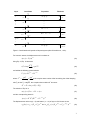
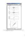
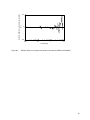
The results of EERA and SHAKE91 are compared for the particular example problem described in
Appendix A. Figures B1 and B2 show the relative difference in EERA results with respect to those of
SHAKE91, including maximum shear strain, maximum acceleration and spectral acceleration. As shown
in Fig. B1, the increase in the relative difference of shear strain close to the free surface results from a
decrease in absolute values of shear strain close to the free surface. As shown in Fig. B2, the increase in
the relative difference of spectral acceleration for large period results from the decrease in absolute
values of spectral acceleration for large period. In this example, the relative difference was found to be
75
75
100
100
125
125
150
150
-0.2
0
0.2
-0.005
0
0.005
Relative difference of maximum
Relative difference of maximum
shear strain (%)
acceleration (%)
very negligible for all practical purposes.
Figure B-1
Relative difference of maximum shear strain and maximum acceleration between
SHAKE91 and EERA
37
Relative difference of spectral acceleration
(%)
0.4
0
-0.4
0.01
0.1
1
10
Period (sec)
Figure B-2
Relative difference of spectral acceleration calculated by EERA and SHAKE91.
38