Download Package `astrochron`

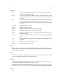
eAsm
21
rayleigh
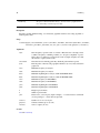
Rayleigh frequency (cycles/m).
nyquist
Nyquist frequency (cycles/m).
sedmin
Minimum sedimentation rate for investigation (cm/ka).
sedmax
Maximum sedimentation rate for investigation (cm/ka).
numsed
Number of sedimentation rates to investigate in ASM optimization grid. Maximum allowed is 500.
linLog
Use linear or logarithmic scaling for sedimentation rate grid spacing? (0=linear,
1=log)
iter
Number of Monte Carlo simulations for significance testing. Maximum allowed
is 100,000.
ydir
Direction for y-axis in plots (depth or height). -1 = values increase downwards
(slower plotting!), 1 = values increase upwards.
output
Return output as a new data frame? (0 = nothing, 1 = Ho-SL, 2 = ASM, 3 = #
astronomical terms, 4 = everything)
genplot
Generate summary plots? (T or F)
Details
Please see function asm for details.
References
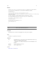
S.R. Meyers and B.B. Sageman, 2007, Quantification of Deep-Time Orbital Forcing by Average
Spectral Misfit: American Journal of Science, v. 307, p. 773-792.
S.R. Meyers, 2012, Seeing Red in Cyclic Stratigraphy: Spectral Noise Estimation for Astrochronology: Paleoceanography, 27, PA3228, doi:10.1029/2012PA002307.
S.R. Meyers, B.B. Sageman and M.A. Arthur, 2012, Obliquity forcing of organic matter accumulation during Oceanic Anoxic Event 2: Paleoceanography, 27, PA3212, doi:10.1029/2012PA002286.
See Also
asm, eAsmTrack and eha
Examples
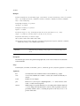
# use modelA as an example
data(modelA)
# interpolate to even sampling interval
modelAInterp=linterp(modelA)
# perform EHA analysis, save harmonic F-test confidence level results to 'spec'
spec=eha(modelAInterp,win=8,step=2,pad=1000,output=4)
# perform Evolutive Average Spectral Misfit analysis, save results to 'res'
res=eAsm(spec,target=c(1/405.47,1/126.98,1/96.91,1/37.66,1/22.42,1/18.33),rayleigh=0.1245274,