1
UoB Earth system modelling workshop: 26th – 27th August 2009
SESSION #1a: GENIE-1 Earth system model basics
A Hitchhikers Guide to the Black Arts
(of Earth system modelling)
SESSION #1a: GENIE-1 Earth system model basics
Stuff to keep in mind:
• GENIE-1 is a model. Models ARE NOT the ‘real World’. (Don’t get confused!)
• The very low (for a 3-D ocean circulation model) resolution of GENIE-1 precludes its explicit
applicability to very short time-scales, and because the simplified atmospheric component
cannot calculate winds, there is no atmospheric dynamics or inter-annual variability.
• GENIE-1 is best thought of as a ‘discovery and exploring’ tool for learning how the Earth
system works rather than a detailed ‘simulation’ tool.
• Have fun (or at least try) ☺
Background reading
The following references provide primary model description and critical evaluation/discussion.
Edwards and Marsh [2005] (Climate Dynamics 24, 415-433)
→ description and calibration of the climate model component of GENIE-1
Hargreaves et al. [2004] (Climate Dynamics 23, 745-760)
→ description of data assimilation methodology and calibrated climatology of the climate model component of
GENIE-1
Ridgwell et al. [2007a] (Biogeosciences 4, 87-104)
→ description of a basic PO4-based carbon cycle in the ocean and calibration of the climate model component of
GENIE-1
Ridgwell et al. [2007b] (Biogeosciences 4, 481-492)
→ description of the calibration and application of the pH-responsive pelagic calcification parameterization
Ridgwell and Hargreaves [2007] (Global Biogeochemical Cycles 21, doi:10.1029/2006GB002764)
→ description and calibration of the sediment model component (‘SEDGEM’) and response to fossil CO2 release
Lenton et al. [2006] (Climate Dynamics 26, doi:10.1007/s00382-006-0109-9)
→ description, calibration, and application of the ‘ENTS’ land surface + vegetation scheme
The following provide a taste of (mostly paleo) applications.
Chikamoto, M. O., K. Matsumoto, and A. Ridgwell [2008] (JGR 113, doi:10.1029/2007JG00066)
→ analysis of the deep-sea CaCO3 sediment and atmospheric CO2 response to Atlantic meridional overturning
circulation shutdown
Panchuk, K., A. Ridgwell, and L. R. Kump [2008] (Geology 36, 315-318)
→ configuration of GENIE-1 for end Paleocene marine carbon cycling; interpretation of the CO2 release associated
with the PETM
Ridgwell [2007] (Paleoceanography 22, doi:10.1029/2006PA001372)
→ description of sediment core modeling in ‘SEDGEM’; application to the interpretation of CCD changes due to
massive CO2 release (e.g., @ PETM)
Singaraye, J. S., D. A. Richards A. Ridgwell, P. J. Valdes, W. E. N. Austin, and J. W. Beck, [2008] (GRL 35,
doi:10.1029/2008GL034074)
→ analysis of the role of changing ocean circulation in atmospheric radiocarbon variability during the Younger Dryas
Copies of these references can be obtained from the ‘usual places’ (i.e., ‘journals’!), or from:
www.seao2.org/pubs.html or http://www.genie.ac.uk/publications/papers.htm.
Other GENIE resources can be found at: http://mygenie.seao2.org.
1
UoB Earth system modelling workshop: 26th – 27th August 2009
SESSION #1a: GENIE-1 Earth system model basics
0.
Before anything else …
0.0
For some of you, the mechanics of running the model will be about as much fun as sticking you tongue in an
electrical outlet ...
GENIE has traditionally been configured and accessed via the ‘command line’ of the linux (or Mac
equivalent) operating system. The command line is a place where you type text and when you press Return,
something (hopefully, good!) happens. Typically the stuff you type started with a ‘Command’ word, and
often followed by one or more options and/or parameters. The Command word and any options / parameters
MUST be separated by SPACEs.
The command line will look something like:
$
The ‘$’ is call the ‘prompt’ and is ‘prompting’ you to type some input (Commands, swear words, etc.). See –
the computer is just sat there waiting for you to command it to go do something (stupid?)!
Often, you will also be informed (reminded) of the username and computer name and current directory at the
prompt, e.g.:
[mushroom@almond ~]$
Which is user ‘mushroom’ on computing cluster ‘almond’ and the current directory is the ‘home’ directory
(~).
Now you can see why people so willingly let Billy Gates suck all their blood in return for a copy of Windoz
... :o)
Read quickly through Appendix 1, which is a quick summary of some of the more important/useful linux
Commands you can use at the command line. You may want to refer to this later.
NOTE: In the following workshop instructions, example lines to be typed at the command line are
highlighted in yellow (or grey when photocopied ...). Be VERY CAREFUL that spaces are not missed out.
Also be careful not to confuse the number one (1) for the letter el (l). Mis-spelling/typing will probably be
the primary reason for any wailing and gnashing of teeth during the workshop ...
But … coming soon is a GUI (graphical user interface) for GENIE that will relieve you of tedious mucking
about at the linux command line. However, in-depth science will always probably be done at the command
line as it give the maximum access to the inner workings of the model and offers the greatest flexibility in
designing experiments.
0.1
DO NOT ‘RACE AHEAD’ AND SKIP OVER BITS THAT YOU CAN’T BE BOTHERED TO READ OR
DO ... IT WILL ALL GO HORRIBLY PEAR-SHAPED BEFORE YOU CAN SAY “WHAT MUPPET
WROTE THESE STUPID INSTRUCTIONS?”.
0.2
Some warnings and reminders are repeated over and over and over and … over again. This is because you
will forget immediately each time! ;)
0.3
Additional documentation can be found on: http://mygenie.seao2.org (under: GENIE resources:
DOCUMENTATION), in particular:
(i) The GENIE User Manual.
(ii) A set of Tutorials.
(iii) A HOW-TO (potted explanations of how to get useful stuff done).
(iv) A table of (namelist) parameters in the model (for controlling what GENIE does).
(v) A Quick-start Guide (referred to later).
0.4
OK – now log into the PC …
2
UoB Earth system modelling workshop: 26th – 27th August 2009
SESSION #1a: GENIE-1 Earth system model basics
1.
Starting off …
1.0
You are going to be installing the model from scratch – why? Why not? Hell, it saves me installing it a dozen
times! Actually, having gone through the install and testing procedure once, you should be able to install
GENIE ‘for real’ another time. (If you dare ever use it again ...)
1.1
Log in to the account that has been created for you on the almond computing cluster. To do this – first start
the SSH Secure Shell program (you can find this via the All Programs menu tree from the Start icon in
Windoz). Run the Secure Shell Client rather than the Secure File Transfer Client to start off.
Click on the Quick Connect icon in the main Secure Shell Client window. A ‘Connect to Remote Host’
dialogue box will appear. In the first box, ‘Host Name’, enter:
almond.ggy.bris.ac.uk
and your computing cluster user-name on the line below this (‘User Name’).
When (and only when) you click on the Connect button will you be asked for your password in a new
dialogue window that will appear.
Don’t get confused between the PC username and password, which will only get you into the Windoz PC,
and the username and password for the computer cluster. There are TWO sets of passwords and usernames.
(Because there are 2 different computers involved.)
You should now have a dull, blank-look window with the command prompt ($) (see previous page). If you
have a window that looks something like a file manager / directory display ... you have mixed up steps 1.2
(below) and 1.1. (Does not matter.)
1.2
For displaying directory contents and transferring model results files we are going to be using the SSH file
transfer program. One of the icons towards the middle of the icon bar in the SSH terminal window you have
opened is called ‘New File Transfer Window’ (it should be the 2nd icon to the right of the search (binoculars)
icon). Click on this to open a file transfer window.
You should now have TWO windows open – a ‘shell’ window (lines of text on an otherwise blank screen)
and a file manager (transfer) window. Ensure that you have both these before moving on.
1.3
The next step is to download and test a copy of the source code for the GENIE model.
The instructions for downloading, installing, and testing the model code are summarized in the ‘Super-quickstart guide’ at the end of this hand-out. Follow all the steps (#1-7) in the ‘Super-quick-start guide’ before
continuing on to 1.4. (A more generic version can be obtained from the ‘mygenie’
(http://mygenie.seao2.org) webpage under GENIE resources: DOCUMENTATION.)
Note: the username and password for accessing the repository where the code lives are different from the
password used to log onto the PC and different from the username and password used to access the
computing cluster (almond). So many different passwords! Don’t confuse them! You will not need the code
repository username and password again (they are used only once to install the model).
Note2: Make sure that you have set the correct permissions to the old_rungenie.sh script (as per the
instructions in the Super-quick-start Guide.
Note3!: To create the required directories (step #7) refer to Appendix 1: linux 101 for the required command
in linux. Or folders can be created using the Secure File Transfer Client (under the Operation menu item).
1.4
Take a moment to familiarize yourself with the contents of your home directory – as an alternative to the
linux command line (Command: ls), consult the (right-hand) display listing in the Secure File Transfer
Client. Note that the file listing in the Secure File Transfer Client does not automatically refresh and newly
created files/directories will not necessarily be displayed – click on the Refresh icon or press F5. I repeat –
the file listing in the Secure File Transfer Client does not automatically refresh. Hence, if in subsequent
experiments you cannot see your results appearing, 9 times (closer to 10 actually) out of 10, it will be
because the Secure File Transfer Client display needs to be refreshed. DON’T FORGET THIS! (I know you
will ...)
3
UoB Earth system modelling workshop: 26th – 27th August 2009
SESSION #1a: GENIE-1 Earth system model basics
You will see that your account contains the following files and directories (the highlighted files and
directories are the ones you have just created or downloaded):
genie
genie_archive
genie_output
genie_forcings
genie_log
genie_userconfigs
old_rungenie.sh
[a directory containing the model source code and input data directory tree]
[a directory containing archived model results]
[a directory containing a set of subdirectories – one for the results of each model
experiment]
[a directory containing a series of sub-directories for applying geochemical
forcings, e.g., prescribing CO2 emissions]
[a directory containing redirected run-time output and error messages]
[a directory containing a series of files configuring specific experiments – one for
each model experiment to be run]
[a run script for the GENIE model]
[Appendix C of the GENIE User Manual (http://mygenie.seao2.org) contains a fuller but more tedious explanation of
the directory structure and file contents as well as a schematic diagram ‘overview’.]
1.5
The final setup step (specific to this workshop) is to instill some files you will be needing for running some
pre-configured experiments. From: http://mygenie.seao2.org and under GENIE resources:
WORKSHOPS and PRACTICAL CLASSES and UoB 26th-27th August 2009 – download the rather
improbably named file: GENIEworkshop.UoB.090826.tar.gz to your local machine (PC) and then using
the file transfer manager, transfer across the home directory (~) of your account on the almond computing
cluster. Extract the contents of this archive by typing at the command line in the Secure Shell Client:
$ tar xfz GENIEworkshop.UoB.090826.tar.gz
If you now view the contents of the ~/genie_userconfigs and ~/genie_forcings directories you will
see that they have been populated with a number of files and subdirectories, respectively.
1.6
Later on you will be editing some configuration files. So now might be a good time to check that you can use
the editor! (You will also be using the same editor to view some of the model output.)
You have two alternative options for editing and viewing text files, depending on whether you are a UNIX
nerd with no life, or prefer anything to do with computers to be wrapped in cotton wool and covered with
dollops of treacle.
EITHER: Use the linux vi application if you are familiar with it. I think that this pretty much sucks as a text
editor and life is far too short and brutal … so we will not bother in this workshop …
OR ... Use a suitable linux-friendly text editor (NOT Micro$oft Notepad) in conjunction with the Secure File
Transfer Client. Just such an editor – SciTE, is provided on the desktop machine.
To set SciTE to automatically open the model configuration files: in the Secure File Transfer Client – go to
Edit, then Settings… and from the SECOND File Transfer section of the list in the left-hand panel (there are
TWO File Transfer section entries and you are after the one near the bottom of the lest), click on the button
for If a file association is missing, use this application to open the file. Then from Program Files on the C
drive of the Windoz machine, find the SciTE editor directory and its program executable inside. Click on OK
to close the Settings dialogue box. Then under File in the main menu: Save Settings.
It should now be possible to double-click on a file in the Secure File Transfer Client and it will open like
magic (almost)! Try opening old_rungenie.sh (in your home directory) in this way. If you edit and save
the file, you will be asked whether you want to transfer it back to the remote machine and also whether you
want to over-write the original file. Simply click Yes to both.
If you log out of Windoz then you may have to re-do these settings …
4
UoB Earth system modelling workshop: 26th – 27th August 2009
SESSION #1a: GENIE-1 Earth system model basics
2.
Running the model (‘interactively’, in a shell window)
2.1
The strategy for running the model is as follows [DON’T TYPE ANYTHING YET … JUST READ THIS
SECTION]: At the command-line ($) in the root (home) of your account, you will be entering in a command
(old_rungenie.sh, so named, because it utilizes the ‘old’ way of configuring and launching the model)
together with a list of parameters that will be passed to the model, and as if by magic the model will run (or
sometimes not):
$ ./old_rungenie.sh #1 #2 #3 #4 (#5)
Now pay attention: there are 4 (FOUR) parameters, separated by S P A C E S that MUST follow the
old_rungenie.sh command on a single continuous line (even if it ‘wraps’ around across 2 lines):
#1
#2
… is the name of the required base configuration (‘base config’) of the model.
We will mostly be using the base config: genie_eb_go_gs_ac_bg initially, which specifies the GENIE1 climate model components: GOLDSTEIN ocean (go) + (GOLDSTEIN) sea-ice (gs) + EMBM
atmosphere (eb) together with ocean (bg) and atmosphere (ac) carbon cycle modules. The ocean
circulation component is configured with 8 vertical levels and is forced with annual average insolation.
This configuration is basically as described in Ridgwell et al. [2007].
… is the full path of the directory containing the user configuration (‘user config’) file (i.e., the file
containing the specification of a particular experiment). In the particular file structure adopted here, it will
be: ~/genie_userconfigs
#3
… is the name of the experiment. There must be a file in the directory specified in parameter #2
(~/genie_userconfigs) with exactly the same name as you enter here for parameter #3.
#4
… is the run length of the experiment in years – this must be entered as an integer (even though GENIE
will actually be treating it as a real).
There is also one optional (5th) parameter:
#5
… is the full path (and name) of any model experiment that you wish to continue on from the end of
(called a 'restart' file). If the 5th (optional) parameter is not passed then GENIE will run from ’cold’. If the
5th parameter is present then GENIE will attempt to run from a previously generated (restart) state.
Restarts will be discussed later ...
The GENIE User Manual and Tutorial documents contain a fuller (and rather more boring) description of
the above, as well as examples of the command line syntax (see: http://mygenie.seao2.org).
2.2
As an example of running the GENIE Earth system model, you are going to start a modern experiment,
similar to the preindustrial experiment described in the GENIE Tutorial. (The relevant configuration files
have already been provided for you.) You will need the following details in order to construct the appropriate
run command:
parameter #1: The base config is: genie_eb_go_gs_ac_bg
parameter #2: The user config directory is: ~/genie_userconfigs
parameter #3: The user config file is: exp1_modern
parameter #4: Run the experiment for eleven years: 11
parameter #5: There is no restart file, and so no 5th parameter needs to be passed …
The full command you need to enter from your home directory then looks like:
$ ./old_rungenie.sh genie_eb_go_gs_ac_bg ~/genie_userconfigs exp1_modern 11
parameter number =
↑ #1
↑ #2
↑ #3
↑ #4
REMEMBER: This must be entered on a single CONTINUOUS LINE. The (single) S P A C E S are vital.
Take care not to confuse an el (‘l’) with a one (‘1’) when typing this in ...
First, you will have to wait a little while, as all the components of GENIE are compiled from the raw source
code (FORTRAN). When it has finished doing this, the model will initialize and carry out some selfchecking. Only then will it start actually ‘running’ and doing something, and at this point you will see output
of the format:
5
UoB Earth system modelling workshop: 26th – 27th August 2009
SESSION #1a: GENIE-1 Earth system model basics
do the looping.....
model year
* pCO2(uatm)
d13CO2
>>> SAVING BIOGEM TIME-SERIES @ year
0.50
285.160
>>> SAVING BIOGEM TIME-SLICE @ year
0.500000000000000
>>> SAVING BIOGEM TIME-SERIES @ year
1.50
>>> SAVING BIOGEM TIME-SERIES @ year
2.50
>>> SAVING BIOGEM TIME-SLICE @ year
*
AMO(Sv)
ice(%)
<SST>
<SSS>
-6.812
13.816
0.211
1.393
295.241
-7.277
13.201
2.247
302.269
-7.580
12.311
4.377
*
<DIC>(uM)
<ALK>(uM)
34.901
2242.457
2363.077
3.545
34.901
2240.918
2363.122
5.279
34.901
2240.016
2363.147
2.50000000000000
>>> SAVING BIOGEM TIME-SERIES @ year
3.50
307.521
-7.786
11.061
5.509
6.633
34.901
2239.376
2363.175
>>> SAVING BIOGEM TIME-SERIES @ year
4.50
311.502
-7.926
9.865
6.078
7.703
34.902
2238.900
2363.205
>>> SAVING BIOGEM TIME-SERIES @ year
5.50
314.638
-8.022
8.935
6.412
8.578
34.902
2238.528
2363.233
>>> SAVING BIOGEM TIME-SLICE @ year
5.50000000000000
>>> SAVING BIOGEM TIME-SERIES @ year
6.50
317.108
-8.085
8.133
6.630
9.317
34.902
2238.239
2363.256
>>> SAVING BIOGEM TIME-SERIES @ year
7.50
319.071
-8.125
7.910
6.736
9.946
34.903
2238.009
2363.276
>>> SAVING BIOGEM TIME-SERIES @ year
8.50
320.618
-8.147
7.936
6.736
10.487
34.903
2237.831
2363.292
>>> SAVING BIOGEM TIME-SERIES @ year
9.50
321.817
-8.155
7.981
6.731
10.963
34.904
2237.695
2363.307
>>> SAVING BIOGEM TIME-SERIES @ year
10.50
322.734
-8.152
8.092
6.858
11.406
34.904
2237.595
2363.319
>>> SAVING BIOGEM TIME-SLICE @ year
10.5000000000000
After ‘do the looping.....’ the very first line contains header information describing the columns of
numbers that follow below. Thereafter, all the lines contain summary information about the state of the
model, with the year (time) at which the values are reported in the first column. The remaining columns
(after model year) are as follows:
– mean atmospheric CO2 concentration (in units of μatm)
– mean δ13C value of atmospheric CO2 (‰) (NOTE: only valid if 13C is selected)
– Atlantic meridional overturning circulation (Sv) (assuming modern continents)
– global sea-ice fraction (%)
– global sea surface temperature ‘SST’ (°C)
– global sea surface salinity ‘SSS’ (‰)
– global mean ocean dissolved inorganic carbon (DIC) concentration (μmol kg-1)
– global mean ocean alkalinity (ALK) concentration (μeq kg-1)
(The choice of what information to display on screen as the model is running is rather arbitrary, but the
chosen metrics do tend to summarize some of the main properties of the climate system and carbon cycle –
for my own personal convenience rather than reflecting any fundamental scientific truth ...)
This information is reported at the same intervals as time-series data (see later & refer to the User Manual) is
saved and is indicated by:
pCO2(uatm)
d13CO2
AMO(Sv)
ice(%)
<SST>
<SSS>
<DIC>
<ALK>
>>> SAVING BIOGEM TIME-SERIES @ year …
Interleaved with these lines are lines reporting the saving of time-slice data (the 2- and 3-D model states –
more of which later and in the User Manual). These appear as:
>>> SAVING BIOGEM TIME-SLICE @ year …
2.3
When the model ends (after 11 years, as per the value you specified at the command line), a bunch more
lines of diagnostics things are reported. If you scroll up the screen of the terminal window you can get back
to where the time-dependent information appears while the model was running. Alternatively, you can run
the model again, but after a few years hit <Ctrl-C> (CONTROL key + ‘C’ key) which will halt the model.
Try both: letting the experiment take its natural course and end after 11 years, and terminating it part way
through (which makes it easier to browse the run-time output).
HINT: Make your Secure Shell Client window full-screen in order for the run-time information to be
formatted properly (and thus fully legible).
Now run the same experiment but this time for 101 years (substitute 101 for 11 as the 4th parameter in the
line where you issue the old_rungenie.sh command).
Just from examining the screen output: how close to steady state does the system appear to have come after
this time? Are all the elements of the Earth system converging at equivalent rates (i.e., SST vs. atmospheric
CO2)? This is something to think about later on – ‘has the model reached steady-state?’ What are the slowest
responding parts of the Earth system?
6
UoB Earth system modelling workshop: 26th – 27th August 2009
SESSION #1a: GENIE-1 Earth system model basics
3.
Submitting experiment ‘jobs’ to a cluster
3.0
This bit is no particular fun at all, but it is a very handy ‘trick’ for running the model in the background, and
maximizes drinking time in the pub vs. sat bored watching a computer screen ☺
3.1
Running jobs interactively is all very well, but there are three important limitations:
1. The connection between your terminal and the server computer running the model must remain
unbroken. Anything more than a fleeting loss of internet connectively may result in the experiment
terminating.
2. You can only run one experiment at a time … unless you want to have thousands of separate Secure
Shell Client windows open? I thought not …
3. Any cluster or computer you are likely to be accessing using a shell will not have many computing
cores, either because it is a single machine with only one or two processors, or if a cluster, by using a
shell you a running on the ‘head node’, which will have similar computing core limitations to running
on a single machine. The more experiments you run simultaneously, the slower they will all run …
3.2
The alternative is to submit your experiment as a ‘job’ to a queuing system which then manages what
compute resources are used to run the model. Once you have submitted the experiment, that is it – you can
go straight to the pub :)
Section 3.4 in the GENIE User Manual explains how to use the queue on the almond cluster you have been
provided with an account on. But for now, just take the suggested options to the qsub command on trust.
(The options following qsub and before old_rungenie.sh re-direct screen output and error messaging to
a file and specify which linux ‘shell’ to assume.)
Run the next experiment (exp2_modern) for 11 years, and submit the experiment as a job to the cluster
queue. Use a command line like:
$ qsub -j y -o genie_log -S /bin/bash
old_rungenie.sh genie_eb_go_gs_ac_bg ~/genie_userconfigs exp2_modern 11
Note that you should not include the ./ bit before old_rungenie.sh (unlike before).
The status of the cluster queue can be checked by:
$ qstat -f
(as detailed in the User Manual). After submitting an experiment, you receive a job number. This number
appears in the first column in the queue status information when you issue a qstat –f command. You
should see your job appear on one of the 8 compute nodes (numbered from 0-0 to 0-7), although it might
briefly be a ‘PENDING JOB’. For an 8-level ocean based configuration of GENIE-1, being run for 11 years,
the job should remain there in the queue for a few good tens of seconds before ‘disappearing’ (your clue that
it has finished, or died …). If you periodically re-issue a qstat –f command you can follow your job’s
progress.
7
UoB Earth system modelling workshop: 26th – 27th August 2009
SESSION #1a: GENIE-1 Earth system model basics
4.
‘Restarts’
4.0
Not much fun here either … but again – an important and time-saving (= increased drinking time!) modelling
technique to learn to use.
4.1
By default, model experiments start from ‘cold’, i.e., the ocean is at rest and uniform in temperature and
salinity while the atmosphere is uniform in temperature and humidity. All biogeochemical tracers in the
ocean have uniform concentrations and/or are zero and there are no biogenic materials in deep-sea
sediments. From this state it will take several thousand years (kyr) for the climate system to reach steadystate, closer to 10 kyr for ocean biogeochemical cycles and atmosphere CO2 to reach steady-state, and
approaching 100 kyr for sediment composition to re-balance weathering. Reaching this the equilibrium state
is called the ‘spin-up’ phase of the model.
There is evidently little point in repeating the spin-up for each and every model experiment that might
similar except in a single detail (e.g., testing a variety of different CO2 emissions scenarios all starting from
current year 2009 conditions). A facility is thus provided for requesting that a ‘restart’ is used – starting a
new experiment from the end of a previous one, usually a ‘spin-up’ that has been run explicitly for the
purpose of generating a starting point (restart) for subsequent experiments to continue on from.
4.2
A restart can be requested by setting the 5th (optional) parameter when entering in the old_rungenie.sh
command. A spin-up of the preindustrial Earth system, based on an 8-level resolution of the ocean model and
near identical to that described in Ridgwell et al. [2007a] is provided: modern_SPINUP (which can be found
in the ~/genie_output directory).
The experiment exp3_modern can be told to use a restart state by adding an appropriate 5th parameter at the
command line, e.g.:
$ ./old_rungenie.sh genie_eb_go_gs_ac_bg ~/genie_userconfigs exp3_modern
101 ~/genie_output/modern_SPINUP
Run the exp3_modern experiment (interactively) using the restart. The run-time output should now look
noticeably different. There should be no (very little) drift in any of the various variable values outputted to
the screen.
8
UoB Earth system modelling workshop: 26th – 27th August 2009
SESSION #1a: GENIE-1 Earth system model basics
5.
Model output
5.1
The first thing to note about output (i.e., saved results files) from GENIE is that every science module saves
its own results in its own sub-directory (and sometimes in very different and difficult-to-fathom ways …).
All the sub-directories of results, plus copies of input parameters and the model executable, are gathered
together in a directory that is assigned the same name as the experiment (and the same as the user config file
name). The overall experiment result directory is located within:
~/genie_output
and will be assigned a directory name something like:
run1_modern
Within this are each module’s results sub-directories.
We will consider primarily only results saved by the ocean biogeochemical module ‘BIOGEM’ (biogem).
The results files will thus be found in:
~/genie_output/run1_modern/biogem
BIOGEM has a flexible and powerful facility of saving results by means of spatially explicit ‘time-slices’,
and as a semi-continuous ‘time-series’ of a single global (or otherwise representative mean) variable. In
contrast, ATCHEM does not save its own results (BIOGEM can save information about atmospheric
composition and air-sea gas exchange) while SEDGEM essentially saves results only at the very end of a
model experiment (BIOGEM can also save the spatial distribution of sediment composition as time-slices as
well as mean composition as a time-series). Furthermore, in order to attain a common format for both ocean
physical properties and biogeochemistry, BIOGEM can save a range of ocean results in addition to
temperature and salinity, such as: velocities, sea-ice extent, mixed layer depth, convective frequency, etc
Time-slices
One of the most informative data sets that can be saved is that of the spatial distribution of properties (such
as tracers or physical ocean attributes). However, saving full spatial distributions (a 36×36×8 array) for any
or all of the tracers each and every time-step is clearly not practical; not only in terms of data storage but also
because of the detrimental effect that repeated file access has on model run-time.
Instead, BIOGEM will save the full spatial distribution of tracer properties only at one or more predefined
time points (years). These are called time-slices. At the specified time points, a set of spatially-explicit data
fields are saved for all the key tracer, flux, and physical characteristics of the system. However, rather than
taking an instantaneous snapshot, the time-slice is constructed as an average over a specified integration
interval (the default is set to 1.0 years).
Time-series
The second data format for model output is much more closely spaced in time. Model characteristics must
then be reducible to a single meaningful variable for this to be practical (i.e., saving the time-varying nature
of 3-D ocean tracer distributions is not). Suitable reduced indicators would be the total inventories in the
ocean and/or atmosphere of various tracers (or equivalently, the mean global concentrations / partial
pressures, respectively). Like the time-slices, the data values saved in the time-series files represent averages
over a specified integration interval (the default is set to 1.0 years).
5.3
View the BIOGEM results directory of one of the two experiments that you ran previously. You should see
the following files:
(i) biogem (is the re-start file created form the run you have just complete, and can be ignored).
(ii) biogem_series_*.res – these are the time-series files (in ASCII / plain text format).
(iii) biogem_year_*_diag_GLOBAL.res – these contain (global diagnostics) summary information and
are saved at the same frequency as the time-slices (also as ASCII / plain text).
(iv) fields_biogem_2d.nc – 2-D fields of ocean and atmosphere properties, as NetCDF.
(v) fields_biogem_3d.nc – 3-D fields of ocean properties, as NetCDF.
9
UoB Earth system modelling workshop: 26th – 27th August 2009
SESSION #1a: GENIE-1 Earth system model basics
6.
Viewing time-series output
6.1
A descriptive summary of all the time-series (biogem_series_*.res) data files is given in the GENIE
User Manual if you are really that bored ... The files of most immediate use/relevance are:
biogem_series_atm_humidity.res
biogem_series_atm_temp.res
biogem_series_misc_opsi.res
biogem_series_misc_seaice.res
biogem_series_ocn_sal.res
biogem_series_ocn_temp.res
6.2
- mean atmospheric (surface) humidity
- mean atmospheric (surface) air temperature
- mean ocean overturning stream-function; Atlantic and global min, max
- mean ocean sea-ice cover and thickness
- mean ocean surface and whole ocean salinity
- mean ocean surface and whole ocean temperature
The contents of the files can be viewed by changing directory into the results directory, i.e.,:
$ cd ~/genie_output/exp1_modern/biogem
and opening a file in the vi editor. But I promised that we would not do anything quite so unpleasant in this
workshop …
Instead – change to the experiment results directory and then to the BIOGEM sub-directory in the Secure
File Transfer Client, and try double-clicking on one of the .res files (listed above). For
biogem_series_ocn_temp.res, you should see 3 columns – time, mean (whole) ocean temperature (°C),
mean (sea) surface temperature ‘SST’ (°C), and mean benthic temperature (°C). Other results files may differ
in the numbers of columns but all should be identifiable from the header information.
6.3
Excel (or MUTLAB if you prefer) can be used to graph the time-series results. Either way you will have to
deal with the header line(s) that are present at the top of the file (and preceding the rows of data).
In Excel: Chose File then Open. You will want to select Files of Type ‘All Files (*.*)’. In the Text Import
Wizard window you can request that Excel skips the first few lines to start the import on the 2nd or 3rd line of
the text file. Alternatively, set appropriate column widths manually in Excel to ensure that the columns of
data are correctly imported.
MUTLAB will ignore lines starting with a %, which the time-series starts with. However, it may be that the
header line wraps-around and there is in effect a 2nd header line but without a %. In this case, extra care (or a
quick edit of the header in the ASCII file) will be required to load the data into MUTLAB.
10
UoB Earth system modelling workshop: 26th – 27th August 2009
SESSION #1a: GENIE-1 Earth system model basics
7.
Viewing time-slice output of 2-D and 3-D environmental property fields
7.1
For the time-slice NetCDF (*.nc) files you will be using a program called Panoply. If you want your own
(FREE!) copy of this utility, you can get it here (and is available for: Windoz, Mac, and linux operating
systems): http://www.giss.nasa.gov/tools/panoply/
7.2
The first time that you try and view a NetCDF file you will need to ‘associate’ the file format (the .nc file
format extension) with the Panoply program. To do this: (1) copy across to a local directory either the 2-D or
3-D NetCDF results file from the BIOGEM results sub-directory, (2) right-mouse-button click over the file,
and chose Open With… , (3) Browse … and find the Panoply program file, select and tick: Always use the
selected program to open this kind of file. Hopefully … all you have to do now is to double-click on the .nc
file icon in the File Transfer window and the time-slice will be displayed like … something that is
“indistinguishable form magic in a sufficiently retarded civilization” (adapted from A. C. Clarke).
When you open the NetCDF file, you will be presented with a ‘Datasets and Variables’ window (on the left
hand side of the application window). This contains a list of all the parameters available that you can display.
You will find that the ‘Long Name’ description of the variable will be the most helpful to identify the one
you want. Simply double-click on a variable to display. For the 3-D fields you will be asked first whether
you want a ‘Lon-Lat’ or ‘Lat-Vert’ plot (for the 2-D fields, the plot display will immediately open).
For the ‘Lon-Lat’ plots – there are multiple levels (depth layers) in the ocean of data that can be plotted, form
the surface to the abyssal ocean.
For the ‘Lat-Vert’ plots – there are multiple possible longitudes to plot slices from. The default is the global
mean meridional distribution.
You can interpolate the data or not (often you may find that it is clearer not to interpolate the data but to
leave it as ‘blocky’ colors corresponding to the resolution of the model), change the scale and colors, overlay
continental outline, change the projection, etc etc. Gray cells represent ‘dry’ grid points, i.e., continental or
oceanic crust.
There may be multiple time-slices (i.e., you can plot data saved form different years).
NOTE: The default settings in Panoply can mislead: (1) the 1st time-slice (often year mid-point 0.5)
rather than the experiment end, (2) auto-scaling of the color scale, (3) global zonal averaging of latdepth plots. Be careful when opening a new plot that you are looking at what you *think* you are
looking at …
7.3
7.4
Explore different data fields and play with different ways of displaying them. Aim for a set of display
properties that show the information you are interested in / want to present in the clearest possible manner.
Try different years (time-slice number), depth level (for a lat-long plot), or longitude (for a vertical section).
Note that gray cells represent ‘dry’ grid points, i.e., continental or oceanic crust.
7.5
To save plots in Panoply:
File
Save Image As …
Then select the location, filename, and graphics format.
7.6
There is also a set of MUTLAB script for plotting the BIOGEM (and SEDGEM) NetCDF output. See:
http://mygenie.seao2.org (under ‘Miscellaneous’). Note that you may need to install MUTLAB NetCDF
libraries (which are invoked by the init_netcdf.m, which note is configured for a specific location of the
library files on a PC and will probably need to be edited appropriately). You are pretty much on you own
here – see the instructions assessable via http://www.giss.nasa.gov/tools/panoply/ for what library files are
required, where to get them from, and where to install them.
11
UoB Earth system modelling workshop: 26th – 27th August 2009
SESSION #1a: GENIE-1 Earth system model basics
Appendix 1 – linux 101
Throughout the GENIE tutorials and documentation, your home directory will be represented by ‘~’. Thus,
for example, the output directory path will be written:
~/genie_output
Viewing directories; moving around the file system
At the command line prompt ($) in linux, you can view the current directory contents:
$ ls
or for a more complete output:
$ ls -la
To go down a directory (genie_output) is:
$ cd genie_output
and to go back up one is:
$ cd ..
You can always return to your home directory (~) by typing:
$ cd
or:
$ cd ~
Copying and moving files
To copy a file myconfig to myconfig_new:
$ cp myconfig myconfig_new
To move myconfig to the GENIE user config directory:
$ mv myconfig ~/genie_userconfigs/myconfig
To rename myconfig to useless_config:
$ mv myconfig useless_config
Creating directories
To create a directory mydirectory:
$ mkdir mydirectory
Repeating command lines
You do not have to re-enter lines of commands and options in their entirety each time – by pressing the UP
cursor key you get the last command you issued. If you keep pressing the UP cursor key you can recover
progressively older commands you have previously entered. When you have recovered a helpful line you can
simply just edit it, navigating along with the LEFT and RIGHT cursor keys (press RETURN when you are
done).
12
GENIE Super-quick-start Guide
Andy Ridgwell
August 25, 2009
1. To get a (read-only) copy of GENIE; from your home directory in the SSH Shell Window (~), type:
$ svn co http://source.ggy.bris.ac.uk/subversion/genie/tags/rel-2-5-0
--username=genie-user genie
NOTE: All this must be typed continuously on ONE LINE, with a S P A C E before ’--username’, and before
genie. You my (or may not!) be asked for a password – if so, it is: g3n1e-user. (Don’t mix up the ONE (’1’)
with an ’el’ (’l’) ...)
2. Change directory (see: Appendix I) to ~/genie/genie-main and type:
$ make
This compiles the default configuration of GENIE. It serves to check that you have the software environment
correctly configured. If you are unsuccessful here ... too bad. Try editing user.mak or user.sh which are located
in ~/genie/genie-main and which set the environment.
3. Next:
$ make assumedgood
This creates a ’gold standard’ set of experimental results for GENIE-2 (GENIE with the dynamical (ICGM)
atmosphere), against which your version of GENIE-2 can subsequently be check to ensure that you have not
broken it in any way.
4. There are a bunch of tests that check the integrity of the code and results, but you can assume that the
tagged-release you have installed has already been extensively checked and is good to go. (The tests are:
make test – short tests that check against your newly created ’assumed good’ experimental results; make
testebgogs – the EMBM-based climate model; make testbiogem – climate model plus ocean biogeochemsitry
(BIOGEM). Because the results of the EMBM-based climate model are not chaotic, these tests compare the
result against a ’known good’ set of results files that are held on SVN and installed along with the code in
~/genie/genie-knowngood.) Run just a single test for now:
$ make testbiogem
There may be some ’Warnings’ reported (== sloppy programming) but these are not detrimental to the ultimate
science results (we hope!). ’Success’ of this test is indicated at the end if you get:
**TEST OK**
and you can then be certain that the model you have installed is producing identical (within tolerance) results
to everyone else in the World who has ever installed GENIE.
5. At this point, the science modules are currently compiled in a grid and/or number of tracers configuration that
is unlikely to be what you want for running experiments. Clean up (remove) all the compiled GENIE modules,
ready for re-compiling afresh from the source code by typing:
$ make cleanall
6. That is it as far as basic installation goes. Except to read the user manual ;) You will be using a script (mini
program, if you like to think of it in that way) that carries out some basic configuration tasks and packages up the
results – old rungenie.sh, which can be downloaded from mygenie.seao2.org, and under ’GENIE resources:
WORKSHOPS and PRACTICAL CLASSES’, the link to: ’UoB 26th-27th August 2009’. This file should be installed
in your home (˜) directory, and MUST have executable permissions (chmod u+x old rungenie.sh). Note that
you run old rungenie.sh from your home directory, NOT ~/genie/genie-main (which confusingly is where
the tests are run from).
7. Finally – for running GENIE-1 using ’rungenie’, create (see: Appendix I) the following directories:
~/genie_archive
~/genie_forcings
~/genie_log
~/genie_userconfigs
1