1
Dear Editor,
We are very thankful for the detailed and constructive comments and recommendations from
Johann Fank and Frederik Schrader. We revised the manuscript carefully and improved it greatly
due to the annotations of the reviewers. Please find our revisions and replies to the reviewers’
comments as inserted text, below.
Andre Peters, Thomas Nehls, Horst Schonsky and Gerd Wessolek
Reviewer #1 (Johann Fank)
General and specific comments:
We are very thankful for the judgment of Johann Fank, all his annotations and the great time effort
he made for testing the routine in detail. The application of our filter routine to his data shows its
general applicability. In general he draws the same conclusion as we do, e.g. that further research is
needed to develop an objective method in order to find the best filter parameters (see our
comments on expert knowledge below).
He also concludes that the filtered results should be compared to independently measured values for
P and ET. We think that this is an impossible task to date, since precision lysimeters are considered to
be the most precise devices with lowest systematic deviations to measure these quantities (see page
14647, line 27 to page 14648, line 3 of the discussion paper).
We also think that estimating the filter parameter δmin by comparing the results with high resolution
precipitation measurements might lead to wrong estimates, since such rain gauges are prone to
systematic errors (see page 14647, lines 10-11 of discussion paper).
In fact, our visual analysis (Figs. 6 and 7 of discussion paper) shows that fixing δmin to a value close to
the measurement resolution gave reasonable results. This selection is confirmed by the fact that δ is
equal to δmin only in cases with no or very low external disturbance. In such a case there is no need to
have values for delta, which are substantially greater than the resolution of the scales. Using higher
values for δmin might lead to an underestimation of both P and ET. From our analysis (Fig. 10 of
discussion paper) we conclude that if δmax is set to a reasonably large value (>0.2 mm), only
parameter wmax has to be predefined by expert knowledge.
It seems to be noteworthy that the reviewer apparently used two different values for the minimum
window width (wmin) in his figure 2. For the case without threshold (δ = 0, blue line) wmin is not set to
1 minute as suggested in our manuscript so that the data of the precipitation events are not well
described. In the case with threshold value (red line), the data are better described due to a smaller
allowed value for w.
Technical corrections:
The data, which have been analyzed stem from a lysimeter without vegetation (see page 14650, lines
12-13 of discussion paper). Thus, in the results section evaporation is correct.
Reviewer #2 (Frederik Schrader)
General comments:
We are very thankful for the judgment of Frederik Schrader and the detailed suggestions he made in
order to improve the manuscript. We considered them carefully and will answer to each of them in
the following.
Specific comments:
p. 14647 l. 6–8: “the flux leaving the soil-plant system towards the
atmosphere within a certain time interval is given by evaporation (E [mm]),
interception (I [mm]) and transpiration (T [mm]), often summed up to
evapotranspiration (ET [mm]).”
Please make it clearer that you mean evaporation of intercepted water and
not the process of interception itself.
The reviewer is right. The sentence was changed to:
“…whereas the flux leaving the soil-plant system towards the atmosphere within a certain time
interval is given by soil evaporation (E [mm]), evaporation of intercepted water (I [mm]) and
transpiration (T [mm]), often summed up to evapotranspiration (ET [mm])”.
p. 14647 l. 11–12: “The reference evapotranspiration (ET0 [mm]) is often
determined with a class-A pan.” Class A pan evaporation is not the same as
(grass) reference evapotranspiration as described by Allen et al. (1998).
Here, the text was mistaken. There is a difference between reference crop evapotranspiration and
the grass reference evapotranspiration. The reference evapotranspiration ET0 is indeed often
determined using a Class A pan and applying a correction which accounts for island effects,
differences in albedo between water and grass, etc. This passage was slightly changed in the new
manuscript: "One method to determine the reference evapotranspiration (ET0 [mm]) is the use of a
class-A pan. Due to differences in albedo between water and grass and island effects, among other
factors, these measured data have to be corrected by a so called pan coefficient (Irmark et al., 2002,
Gundekar et al., 2008), which is location dependent (Howell et al., 1983)”
p. 14647 l. 18–19: “In order to determine P and ET, the masses of lysimeter
and seepage water have to be measured in high temporal resolution.”
Please elaborate on why this is necessary, since traditionally, lysimeter
water balances were often evaluated much less frequently than 1 min−1. I
suppose it would be helpful for some readers to explain why this is (or is
not) a bad idea and why calculating the mass balance, for example, between
two measurements 30 min apart can be significantly different from
calculating a 30 min mass balance using 1 min measurements. A brief
discussion on definitions would be a valuable addition to this. For
example, should we count small precipitation events that evaporate almost
immediately and are not recorded by low-frequency sampling systems in longterm water balances? Where do we draw the line between negligible and
significant events? Which time scales are of practical interest and which
are of interest for researchers? All of these are fundamental questions
that have to be discussed with the increasing availability of highfrequency, high-precision measurement devices. I do, however, understand if
the authors deem this discussion beyond the scope of their rather technical
paper.
We agree with the reviewer on the importance of these questions, and that this discussion would
sidetrack from the general line of the paper. However, we slightly changed and supplemented that
part to account for these questions in a rather general way: “In order to precisely distinguish
between P and ET, which might occur both in relatively small time intervals, the masses of lysimeter
and seepage water have to be measured in high temporal resolution. This is of special importance if
the energy balance of the soil-plant atmosphere system is focused, where a great fraction of total
heat flux is given by latent heat flux (Foken, 2008). Note that for long term water balances focusing
on e.g. ground water recharge, where a precise discrimination of P and ET is not needed, a high
temporal resolution of measurements is not necessary.”
p. 14648 l. 4–5: “small mechanical disturbances (e.g. caused by wind)”
and p. 14649 l. 11–12: “in periods with low wind speed the data are more
accurate than in periods with high wind speed”
Just out of curiosity: Have you seen this in your data (should be
relatively easy to test), or is this an assumption?
We could indeed see this in our data. Moreover, this correlation was found and published for
example by Nolz et al. (2013), which is cited in the manuscript. We put this citation now in the
second sentence: “Moreover, in periods with low wind speed the data are more accurate than in
periods with high wind speed (Nolz et al., 2013).”
Do you believe that this noise is always symmetric around the mean signal?
Using local regression or moving average filters makes it appear so during
residual analysis, but this does not necessarily need to reflect the true
nature of the stochastic errors.
We assume that disturbances caused by wind are not necessarily symmetric. Wind might lead to
temporally different air pressures above the lysimeter as compared to the lysimeter cellar, which in
turn might lead to slightly systematic lower or higher values for lysimeter weight in such wind events.
However, as strong wind events do also lead to higher disturbances, such a small systematic effect
will not be accounted for in our data analysis due to the accompanied low resolution, which is
reflected in a higher threshold value during such events. As higher wind speeds will lead to greater
systematic effects, the graph for the strong wind event in Figs. 6 and 7 might be helpful: There, we
can hardly see a systematic effect but a very high data noise. Lower wind speeds will lead to lower
noise but also to lower systematic effects.
To clarify this point we introduced a short paragraph in the conclusions section: “It is noteworthy
that noise caused by wind is not necessarily symmetric around the mean signal. Wind might lead to
temporally different air pressures above the lysimeter as compared to the lysimeter cellar, which in
turn might lead to slightly systematic lower or higher values for lysimeter weights in such wind
events. However, strong wind events do lead to greater noise, which leads to higher threshold values
(Eqs. 5 and 8). In the strong wind event (Figs. 6 and 7), a systematic effect is hardly visible. Lower
wind speeds will lead to lower noise but also to lower systematic effects. Thus, a small systematic
effect due to wind will not be accounted for in the analysis.”
• p. 14648 l. 9: “the measurement noise is not a constant value”
Please rephrase. If noise was a constant value, it would not be noise but a
systematic error.
Thank you for that comment. We rephrased the sentence: “Moreover, as the wind speed varies with
time, the measurement noise is also varying with time”
p. 14652 l. 1: “The typical way to filter noisy lysimeter data is (i) to
introduce a smoothing routine, like a moving average with a certain
averaging window w, and then (ii) to apply a certain threshold value δ,
accounting for measurement”
While this is a reasonable approach, I don’t think I would call it “the
typical way”. In fact, I would argue that, as of writing this review, there
is no such thing as a “standard method” for the estimation of P and ET from
weighing lysimeter data. Often the mass balance is evaluated at intervals
greater than 1 min, where noise is certainly present, but not as apparent
as in high-frequency measurements. In a few cases, this is preceded by
slight smoothing using a simple moving average, a Savitzky-Golay filter,
or, less common, Wavelet denoising. However, I am not aware of cases where
a smoothing-and-thresholding procedure was applied that were not published
relatively recently.
The reviewer is certainly right with this statement. We slightly changed “the typical way” by “a
promising approach” in that sentence as well as in the abstract and the introduction.
p. 14652 l. 20: “Data with small noise (smooth evap in Fig. 2) need a small
value for δ”
I don’t think so. The choice of a suitable threshold parameter is a
tradeoff between noise-canceling and signal-preserving properties. Since,
in this case, less noise has to be canceled, the threshold parameter can be
smaller, but it certainly does not need to be. In fact, if the threshold is
too low, one may count, for instance, autocorrelated errors that are
“traced” by the smoothing algorithm, as significant.
We absolutely agree that the threshold value should not be too small. Therefore, we suggest a
minimum threshold value slightly above the scale resolution. This minimum threshold value is only
reached in cases with no or very low noise. Note that our filter is a combination of two parts
(smoothing and “thresholding”). Autocorrelated errors due to the smoothing algorithm are only of
relevance if strong signals are smoothed with a relatively large window width. This is prevented by
our smoothing routine, which has a small window width for such strong signals. In such a case the
autocorrelated errors from a moving average are negligible.
The thresholding procedure is, from my experience, very robust in terms of
sensitivity to high values of δ (but it does have a cut-off point when δ is
too low, i.e. when it falls below the noise).
For sure the procedure is less robust for very small values of δ. Such small values for δ have not been
applied in this study, since it is obvious that δ should be larger than scale resolution. Although too
large fixed values for δ are less severe, they do lead to loss in accuracy (see Fig. 7 in the manuscript
and red dashed line of Fig. 1 in this author comment document)
p. 14653 l. 5–6: “Second, a moving average with adaptive window width is
applied” Why did you decide to use a moving average, despite its poor
spike-preserving properties? A Savitzky-Golay filter would not be much more
computationally expensive, since it is only numerically equivalent to the
center point of a local polynomial regression, but mathematically
equivalent to a weighted moving average (Press, 1992).
The choice of the moving average (MA) was not made due to the computational expense but due to
the oscillation behavior of the Savitzky-Golay (SG) filter when strong signals occur, i.e. in heavy rain
events (see figures 6 and 7). This bad performance of the SG algorithm was also reported by Bromba
and Ziegler (1981). Moreover, the poor spike-preserving properties of the MA algorithm do only
occur with relatively large window widths. Spikes are strong signals, which lead to small window
widths (Eq. 7), so that the above mentioned problem cannot occur with our approach.
p. 14653 l. 8: “the software is available from the authors”
Why not directly release it as supplementary material then?
The software is available upon request. The main reason is that there is neither a user friendly
interface nor a user’s manual, yet. Thus, in order to use the software, a contact with the authors is
mandatory anyway.
p. 14653 l. 16: “The order of the polynomial must be high enough to
guarantee that it can describe the data in the time window reasonably well”
What would be the practical implications of just using a straight line fit?
From what I understand, a lower-order polynomial would lead to only
slightly lower moving windows and slightly higher threshold values, both of
which I see nothing wrong with. Fitting kmax polynomials and calculating a
model selection criterion for each point seems unnecessarily impractical
and computationally expensive to me.
Inspired by the reviewer’s idea, we tried using a first order polynomial. For strong signals, this
simplification will lead to larger values for the window width and thus to less accuracy (see Fig. 1 of
this document, right, green solid line and red dashed line). Thus, we keep using higher order
polynomials to get better results. We added the following sentence to the end of section “3.3.2
Calculation of adaptive width of moving window”: “Note that a too low order of the polynomial (e.g.
kmax = 1 would lead to larger window widths and thus to less accuracy for strong signals like the heavy
precipitation event (data not shown).”
p. 14655 l. 8–11: “This is especially important, when the amount of data to
be filtered is large. In this study we used approximately 2×10⁵ data
points, meaning that 2 × 10⁵ polynomial fits had to be conducted.”
Actually it would be kmax × ndata fits, i.e. 1.2 × 10⁶ in this particular
case, not to mention the additional calculation of Akaike’s information
criterion (although that part may be negligible). This is another reason
why I would recommend investigating the consequences of simply using a
straight line fit.
Thank you for that comment. We changed the according part in the revised manuscript. About using
a straight line fit see the reply above. Therefore, the calculation effort should not be reduced as it
can only be reduced with a loss of accuracy.
p. 14655 l. 21–22: “wmax for events with no evaporation or precipitation”
It is in the nature of your approach that only the “intensity” and not the
duration of a signal is considered. For example, an absolutely straight
line with a nonzero slope (e.g. a constant evaporation rate over a long
time) does not get smoothed with w = wmax, although this would be
preferable. Do you have an idea how to solve this problem?
We do not think that it is preferable to smooth a straight line, i.e. a signal without any noise.
However, any signal is accompanied with some noise due to scale resolution, even without any
external disturbances. If a smooth evaporation is accompanied with some noise, the window width
becomes larger. See a, b, c in Fig. 4 and Tab. 1. It should also be mentioned that evaporation gives a
relatively low signal with a maximum of approximately 1 mm/h (van Bavel and Hillel 1976), so that
little noise will lead already to low values for B and thus to large window widths. This statement was
added at the end of subsection “3.3.2 Calculation of adaptive width of moving window”
p. 14657 l. 8: “For all three filters, the threshold value was 0.081mm”
As you mention in p. 14659 l. 4–6, this value is probably a bit too small.
I would assume that choosing a threshold value slightly too high would have
less negative implications than choosing one slightly too low. Therefore, I
believe that adding the case of δmin = δmax = 0.24mm, i.e. an AWCT (adaptive
window, constant threshold), to this comparison would be very interesting.
This is indeed an interesting thought. We chose the value of 0.081mm based on scale resolution of
0.08. Using a higher constant threshold value will certainly lead to a smaller overall error compared
to a low constant threshold value. However, in that case ET and P will be underestimated. See Fig. 1
of this author comment, left and center yellow and red dashed lines. We account for that in the
revised manuscript by introducing the following sentence in section “4.2 Test of AWAT filter with
variable w and δ“:“Using a constant value of δ = 0.24mm for the AWAT filter leads to the same
disadvantages as for the MA and SG filters (not shown).”
p. 14657 l. 27–p. 14658 l. 1: “The strong wind event is better described by
the AWAT filter as by the SG filter and equally well as by the MA filter”
How do you know?
By visual inspection of Fig 6 combined with the information that during the strong wind event no
precipitation took place (see p. 14657, l. 13-14 of discussion paper). This information is now added to
the material and methods section of revised manuscript.
p. 14658 l. 18–19: “not perfectly filtered anymore”
Unfortunate choice of words, in my opinion. Implies that you have a measure
of perfectness and that your filter performs perfectly during certain
situations.
The reviewer is right. We rephrased that sentence as follows: “Even in case of wmax = 61min, the new
filter is well suited, although the data of the heavy precipitation event are now filtered slightly
worse.”
p. 14659 l. 1: “residuals are more or less normally distributed”
Have you tested this? If not, “symmetrically” would probably be a more
suitable wording.
Again, the reviewer is right. We rephrased that sentence as follows: “In that case the residuals are
more or less symmetrically distributed with zero mean.”
p. 14659 l. 12–13: “as long as a change from ti−1 to ti is regarded to be
insignificant, the value for ti−1 is kept”
This should be in the methods section, not in the results. The explanation
in p. 14652 l. 16–19 is somewhat short anyway. It should be described in
more detail how this is not simple thresholding, but what I would call
“thresholding with memory” (which is necessary to preserve the shape of the
cumulative signal).
We wrote this short section solely to explain the shape of the residual distribution and thus would
like to keep that sentence here. Additionally, we followed the advice of the reviewer and extended
the according paragraph in section “Separating P and ET from noise - general approach”: “After
smoothing, there is usually still some noise left (Fig. 2, center panel), which would lead to an
overestimation of both P and ET. Therefore, a threshold value, δ [mm] is introduced to reduce the
fluctuations (Fig. 2, right panel). The threshold approach, which might more correctly be named
"thresholding with memory", makes sure that significant weight changes are separated from
insignificant changes, in a way that all changes in weight smaller than a pre-defined accuracy
threshold δ are discarded. As long as a change from ti-1 to ti is smaller than δ, the value for ti-1 is kept.
Such a threshold value should be at least as high as the scale resolution.
p. 14659 l. 14–15: “This leads to an underestimation, and thus to negative
residuals for evaporation events and to an overestimation and thus positive
residuals for precipitation events. ”
I would humbly suggest performing the residual analysis only for those ti
at which a change in mass was counted as significant, or to find a suitable
interpolation procedure between two such points, in order to eliminate the
step-like shape of the reconstructed signal.
About interpolation: We think that the step like shape is the most trustable reflection of the
measurement accuracy. To our point of view, any interpolation procedure, which leads weight
intervals smaller as the measurement accuracy is mere speculation. Thus we keep the filtered signals
without interpolation.
The residual analysis was performed to get information on how the smoothing and threshold
routines yield biased results. With this aim it must be performed for each point in time. If the analysis
is done only with those ti at which a change in mass was counted as significant there will be no such
bias. This is because at those times the reconstructed signal with applied threshold value hits the
mere smoothed signals by definition (see red circles in Fig. 2 in this document). Thus, any systematic
underestimation of either precipitation or evapotranspiration would not be reflected.
p. 14660 l. 7–9: “The fluxes estimated with the SG filter can even increase
as w increases. This might be due to the fact that the SG filter tends to
oscillate”
Very true and important statement, and even more obvious when using
nonadaptive procedures. From my experience, a rather narrow w and a
sufficiently large δ generally yield satisfying and robust results, though.
I found δ to be relatively robust if larger than a certain cut-off point
(which is lower than the noiseintensity itself). That was, however, only
tested using fully synthetic data and measurements from a modern lysimeter
with three precise load cells, not a leverarm counterbalance system that is
known to exhibit stronger and oscillating noise
(e.g. Nolz, 2013).
We found out that using small values for w and larger ones for δ will result in some kind of accuracy
loss (see Fig. 1 of this document). Thus we prefer to keep the routine as it is.
p. 14661 l. 3–4: “it is not recommended to use the Savitzky–Golay filter
for evaluating lysimeter data”
I found this statement a bit too generalized to be derived from a single
study on very specific events, measured with a lysimeter featuring a
somewhat dated weighing technology.
Here we disagree with the reviewer. The problem of oscillation of the SG filter has nothing to do with
the measurement system. It is due to the very strong signals, which are given by heavy precipitation
events. Any strong signal (heavy precipitation) would yield a similar behavior if the window width is
not very narrow. This is in accordance to the findings of Bromba and Ziegler (1981).
We agree that our study is a case study with limited data. However, the three benchmark events
were chosen very carefully. They represent very characteristic events. If the SG filter is not working
properly for one of these three events, it is likely that there are several other evens for which the SG
filter does not work as well. Thus we keep to our recommendation that the SG routine should not be
used any longer for evaluating lysimeter data.
p. 14661 l. 8–10: “Figures 6 and 7 show that δmax = 0.24mm was a much better
choice than δmax = 0.081 mm. Thus, it is concluded that δmax can be set to any
reasonably high value.”
Alternatively the variable threshold procedure could simply be omitted. I
found it difficult to compare those two cases, since one is AWAT and one is
AWCT. Again, these would be easier to compare if you examined a case where
δmin = δmax = 0.24mm.
See our reply above and Fig 1 (red and yellow dashed lines in left in center panels) of this author
comment. The accuracy as given in Fig 7 is only possible if δmin is set as small as possible (close to
scale accuracy) and δ is allowed to vary in dependence to noise.
p. 14661 l. 13–14: “Choosing wmax carefully with expert knowledge”
Or trying to derive it from the data, leading to a fully adaptive filtering
method. But such methods have to be tested thoroughly using both synthetic
and real data that feature a broad range of meteorological conditions.
We suggest the testing with synthetic data as well in the last sentence. A fully adaptive filtering
routine would be helpful. However, we doubt that such an algorithm, including the complete
relevant expert knowledge, can be achieved in the near future. Moreover, “expert knowledge” itself
is an adaptive procedure and is improved as more data is processed and better filter routines are
available. Thus, we strongly recommend to always check time series describing such complex system
behaviors like boundary fluxes at lysimeter surfaces, before and after filtering with expert
knowledge.
p. 14661 l. 15: “For our benchmark events, including very different
atmospheric conditions, wmax = 31 min led to the best results.”
This is in agreement with my own experiences.
That is an interesting statement. Future research on the physics of soil-atmosphere boundary fluxes
will show how general this information is.
Whole document: ET should be typeset like all other water balance
variables. Either make the other variables upright as well, or use the
mathit command to typeset slanted variables with multiple capital letters
without too much space between them.
This was a typesetting problem in the production phase. Because of the journal's guidelines, we set
the other variables upright as well.
p. 14648 l. 11: “up to 5 times”
Small numbers should be spelled out, i.e. “up to five times”, as you did in
the preceeding line.
Has been changed
Figures
Fig. 1: The three benchmark events with different AVAT filter settings. δmin =0.081: AVAT filter with
variable δ and with δmax = 0.24 mm; δmin = 0.24: AVCT filter with δmin = δmax = 0.24mm; kmax = 1:
Polynomial is given by straight line; kmax = 6: Order of polynomial depends on AICc as in manuscript.
wmax is in all cases 31 min.
Fig. 2: The strong wind event with the three different filters. Blue line: Mere smoothing without
threshold; red line: filter with threshold; red circles: filtered data at time ti where changes are
regarded as significant. w and wmax, are in all cases 31 min and δ and δmax are 0.24 mm.
References
Bromba, M. and Ziegler, H.: Application hints for Savitzky–Golay digital smoothing filters, Anal.
Chem., 53, 1583–1586, doi:10.1021/ac00234a011, 1981.
Foken, T.: The energy balance closure problem: An overview, Ecol. Applications, 18, 1351–1367,
doi:10.1890/06-0922.1, 2008.
Gundekar, H. G., Khodke, U. M., Sarkar, S., and Rai, R. K.: Evaluation of pan coefficient for reference
crop evapotranspiration for semi-arid region, Irrig. Sci., 26, 169–175, doi:10.1007/s00271-007-0083y, 2008.
Howell, T. A., Phene, C. J., and Meek, D. W.: Evaporation from screened Class A pans in a semi-arid
climate, Agric. Meteorol., 29, 111–124, doi:10.1016/0002-1571(83)90044-4, 1983.
Irmark, S., Haman, D. Z., and Jones, J. W.: Evaluation of Class A pan coefficients for estimating
reference evapotranspiration in humid location, J. Irrig. Drain. Eng., 128, 153–159,
doi:10.1061/(ASCE)0733-9437(2002)128:3(153), 2002.
Nolz, R., Kammerer, G., and Cepuder, P.: Interpretation of lysimeter weighing data affected by wind,
J. Plant Nutr. Soil Sci., 176, 200–208, doi:10.1002/jpln.201200342, 2013.
van Bavel, C. H. M. and Hillel, D. I.: Calculating potential and actual evaporation from a bare soil
surface by simulation of concurrent flow of water and heat, Agric. Meteorol., 17, 453–476,
doi:10.1016/0002-1571(76)90022-4, 1976.