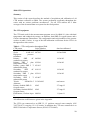
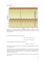
1
JR84 Cruise Report
Autosub Under Ice Cruise
to the Amundsen Sea
RRS James Clark Ross
28 February to 4 April 2003
Report complied by Adrian Jenkins
from the contributions of the scientific party:
Chris Banks, Toby Benham, Mark Brandon, Jon Copley, Julian
Dowdeswell, Jeff Evans, Sarah Hardy, Dan Hayes, Adrian Jenkins, Steve
McPhail, Nick Millard, Colm O’Cofaigh, Miles Pebody, James Perrett,
Ziggy Pozzi-Walker, James Riggs, Pete Stevenson, David Vaughan and
Andy Webb.
Contents
Introduction
Summary
Scientific Party
Ship’s Personnel
Chronological outline of cruise
Sea ice conditions in the Amundsen Sea during JR84
Outreach activities
Marine Geophysical Investigations
EM120
TOPAS
EPC chart recorder
XBT’s
Simrad EA500 Bathymetric Echo Sounder
Sea Ice Observations
Sea Ice Drifters
Physical Oceanography
JR84 CTD operations
SBE43 dissolved oxygen sensors
Appendix: Calibration data
Oceanlogger (Underway Measurements)
ADCP Measurements
Summary
The configuration of the ADCP
Standard method of processing
Identification of CTD ‘on station’ ADCP data
Navigation Data
The instruments
Daily navigation processing
Microbiological Sampling
Autosub Operations
Trim and ballast
Edgetech FS-AU sub-bottom profiler
Simrad EM2000 multibeam swath system
AquaLAB
Autosub SBE 9+ CTD
ADCPs and navigation
Mission descriptions
Connector problems
Damage sustained during recovery after mission 319
Summary of problems encountered during cruise
Autosub Data Analysis
Edgetech FS-AU sub-bottom profiler
Assessment of Simrad EM2000 multi-beam sonar
Autosub under ice missions
CTD, water sampler and ADCP
Cruise Track Plots
2
2
3
4
5
8
10
11
20
23
24
24
26
27
29
30
33
46
47
50
51
51
51
52
59
62
62
67
68
70
72
75
76
78
81
83
85
88
89
92
98
98
108
113
122
128
1
Introduction
Adrian Jenkins (PSO), British Antarctic Survey
Summary
JR84 was the first cruise of the NERC Autosub Under Ice (AUI) thematic
programme. The aim of the programme is to investigate the marine environment of
floating ice shelves in Antarctica and Greenland using Autosub, the autonomous
submersible vehicle developed at the Southampton Oceanography Centre. The target
area for the first cruise was Pine Island Bay, in the eastern Amundsen Sea, with the
main focus being autosub deployments beneath Pine Island Glacier.
Cruise participants included the Autosub technical team, the AUI science coordinator
and scientists working on four separate projects funded by the programme:
Evolution and impact of Circumpolar Deep Water on the Antarctic continental shelf
— Principal investigator: Adrian Jenkins, British Antarctic Survey.
Autosub investigation of ice sheet boundary conditions beneath Pine Island Glacier —
Principal investigator: David Vaughan, British Antarctic Survey.
Marine geological processes and sediments beneath floating ice shelves in Greenland
and Antarctica: investigations using the Autosub AUV — Principal
investigator: Julian Dowdeswell, Scott Polar Research Institute, University of
Cambridge.
Sea ice thickness distribution in the Bellingshausen Sea — Principal investigator:
Mark Brandon, Open University.
The planned activities for the cruise included Autosub missions beneath Pine Island
Glacier, neighbouring glacier tongues and the multi-year sea ice that was expected to
be present to the west of the bay. Planned activities for the ship included CTD
measurements and swath mapping in Pine Island Bay and the neighbouring
continental shelf, as well as measurements on ice floes and the deployment of three
Argos beacons in the multi-year pack.
In case of sea ice conditions in the Amundsen Sea barring access to Pine Island Bay,
most of these activities could have been moved to either Ronne Entrance or
Marguerite Bay, with George VI Ice Shelf becoming the main focus for Autosub
work. Failing this other alternatives, including Larsen Ice Shelf had been identified.
In the event, sea ice prevented the ship getting within 100 miles of any ice front, so
the only under ice Autosub missions were run beneath multi-year sea ice to the north
of Thurston Island. Technical problems with the vehicle meant that these were
somewhat limited in scope and extent. Ice floe sampling and the deployment of the
drifters were also completed in the same area. The remaining shipboard activities
focussed on a seabed trough that cut the Amundsen Sea continental shelf break at
113–115ºW. The marine geological interest here was in the connection of the trough
to the deep inner shelf regions near Pine Island Bay and the record of past ice stream
activity. From an oceanographic viewpoint the trough appears to act as a conduit by
which warm Upper Circumpolar Deep Water is guided onto the shelf and possibly
flows all the way to Pine Island Bay.
2
Scientific Party
Personnel from British Antarctic Survey, Natural Environment Research Council
(High Cross, Madingley Road, Cambridge, CB3 0ET):
Pat Cooper
Dan Hayes
Adrian Jenkins
Jeremy Robst
David Vaughan
Doug Willis
Electronics
Oceanography
Oceanography
Computing
Glaciology
Computing
Personnel from Southampton Oceanography Centre, University of Southampton
(Waterfront Campus, European Way, Southampton, SO14 3ZH):
Jon Copley
Steve McPhail
Nick Millard
Miles Pebody
James Perrett
James Riggs
Pete Stevenson
Andy Webb
AUI Science Coordinator
Autosub
Autosub
Autosub
Autosub
Autosub
Autosub
Autosub
Personnel from Department of Earth Sciences, The Open University
(Walton Hall, Milton Keynes, MK7 6AA):
Chris Banks
Mark Brandon
Sarah Hardy
Ziggy Pozzi-Walker
Sea ice
Oceanography/Sea ice
Oceanography
Oceanography
Personnel from Scott Polar Research Institute, University of Cambridge
(Lensfield Road, Cambridge, CB2 1ER):
Toby Benham
Julian Dowdeswell
Jeff Evans
Colm O’Cofaigh
Marine geology
Marine geology
Marine geology
Marine geology
3
Ship’s Company
Officers:
Christopher Elliott
Robert Paterson
Andrew Liddell
Michael Golding
John Summers
Charles Waddicor
David Cutting
Vincent Blocke
Gerard Armour
Steven Eadie
Simon Wright
Norman Thomas
Kenneth Olley
Master
Ch/Off
2/Off
3/Off
Dk/Off
R/Off
C/Eng
2/Eng
3/Eng
4/Eng
D/Eng
Elect
Cat/O
Crew:
George Stewart
David Williams
John McGowan
Marc Blaby
Derek Jenkins
David Rees
Lester Jolly
Mark Robinson
Sydney Smith
Richard Turner
Raymond Collins
Clifford Pratley
Derek Lee
Kenneth Weston
James Newall
Bosun
Bos/Mate
Sea 1
Sea 1
Sea 1
Sea 1
Sea 1
M/Man
M/Man
Ch Cook
2nd Cook
S/Stwd
Stwd
Stwd
Stwd
Ship’s Doctor:
Alex Ramsden
4
Chronological outline of cruise
28 Feb 2003: JCR departed Port Stanley, Falkland Islands, at 09:00L. We headed for
S54°30’, W059°35’ to commence a swath bathymetry and towed
magnetometer section across Drake Passage. The ocean logger and ADCP
were also running.
1 Mar 2003: We completed the Drake Passage section and commenced our transit to
Gerlache Strait. Underway systems were running throughout the passage.
2 Mar 2003: In transit.
3 Mar 2003: We arrived in Dallmann Bay early in the morning. Autosub passed its
buoyancy test in calm waters among the Melchior Islands. The ship
proceeded to Gerlache Strait for the first Autosub trial missions (M307/8).
We ran a swath survey in Gerlache Strait overnight.
4 Mar 2003: The swath survey finished in the morning, ready for a further Autosub
trial (M309) run. A CTD test cast (001) was run during the Autosub mission.
After the vehicle was recovered, the ship left Gerlache Strait via Neumayer
Channel to start the transit to Peter I Island.
5 Mar 2003: In transit. Underway systems logging.
6 Mar 2003: In transit. Argos drifters were activated on the after deck.
7 Mar 2003: The ship passed Peter I Island early in the morning and headed for sea
ice north of Thurston Island.
8 Mar 2003: We found the ice edge at first light and located a suitable site for an
Autosub deployment (S70°27’, W102°09’). The aim was to test the vehicle to
full depth in open water before commencing the sub-ice missions. Mission
M310 was run coincident with CTD cast 002. The Autosub mission was
aborted part way through and the vehicle was recovered to investigate the
problem. The ship headed into ice to deploy the first drifter on a floe at
S70°59’, W101°10’. Snow and ice thickness were measured on the floe. The
ship then returned to the ice edge and ran a swath survey overnight.
9 Mar 2003: A further Autosub test mission (M311) in the morning revealed a
continuing problem and was aborted almost immediately. We entered the ice
again to deploy the two remaining sea ice drifters and sample the floes near
S70°55’, W102°10’. The ship once again returned to the ice edge and ran a
further swath survey overnight.
10 Mar 2003: Autosub test mission (M312) failed at depth. A full ocean depth CTD
cast (station 003) was run. At midday local time the ship headed further west
to access Pine Island Bay along the W106° meridian.
11 Mar 2003: The ship’s track was pushed further west because the sea ice extending
west from Thurston Island was blocking the intended route. We begin
heading south along W111°.
12 Mar 2003: Our southerly progress was halted overnight when we encountered sea
ice and icebergs. At first light we continued southward along a narrow
corridor between the sea ice to the east and a line of icebergs coming from
Thwaites Glacier to the west. New ice was forming all around the ship. The
ship turned north through the heavier ice to test the condition of the tongue
that could potentially block off our retreat from the Bay. The ship ran a swath
survey outside the ice overnight.
13 Mar 2003: Another Autosub deployment (M313) ended with similar problems.
We started a five station (004-008) CTD section perpendicular to the
continental slope.
5
14 Mar 2003: The CTD section was completed overnight and the ship returned to
deep water for another Autosub test in the morning (M314). It was decided
that the continuing freeze-up to the south and the westward movement of the
ice from Thurston Island put operations in Pine Island Bay out of the question.
We moved westward (to W110°) overnight, broadening the swath survey
along the continental slope.
15 Mar 2003: At first light the ship moved out to deep water to start another CTD
section (stations 009 and 010) across the continental slope. Autosub was
deployed at the second station (M315), but the systems cut out at depth. The
Master was unhappy about continuing the CTD section into the ice at night, so
the ship headed for W113°20’ (where a trough cutting the shelf edge had been
identified in 2000), taking a line well north of the ice edge. A CTD section
across the slope was started.
16 Mar 2003: Overnight the five station (011-015) CTD section was completed. We
then returned to deep water along a track that maximised the swath coverage.
Autosub mission (M316) encountered further problems at depth, so we
recovered the vehicle and headed south onto the continental shelf as far as we
could while staying well clear of ice for overnight operations. We located the
western edge of the seabed trough near W114°15’ and started a swath and
CTD line (stations 016-024) across it.
17 Mar 2003: The transect across the trough was finished by morning and we headed
for the 2000 m isobath at W114°. Autosub completed another two test
missions (M317/8), which left the technical team feeling that most of the
problems were solved for missions to a few hundred metres depth. We started
another CTD section (stations 025-029) across the shelf break. With this
complete an extensive swath survey was started, aimed at mapping the
seaward end of the trough and the upper continental slope beyond.
18 Mar 2003: In the morning the swath survey was suspended for an Autosub test
mission (M319) involving dives to increasing depth, to establish a safe depth
limit for vehicle operations. The mission was successful, but during recovery
in strengthening winds Autosub was knocked by the ship, causing damage to
both the vehicle and some of its sensors. The swath survey continued for the
remainder of the day and into the night.
19 Mar 2003: The swath survey of the trough was completed by morning and the
ship returned to the 2000 m isobath at W113°40’, to run another CTD section
(stations 030-035) up onto the shelf. The swath mapping of the upper slope
was used to place two of the stations over the deep gullies that descend from
the mouth of the trough. With this complete the ship started on a swath survey
of the upper continental slope as far west as W115°.
20 Mar 2003: Part way along the return leg of the swath survey the ship headed out
to the 2000 m isobath to commence a final CTD section (stations 036-040)
back onto the shelf. With this complete the ship headed south to find calm
water within the pack ice for a buoyancy test on the repaired Autosub. With
the buoyancy checked the vehicle was sent on a successful dive to 300 m and
back (M320). Movement of the ice forced a recovery of the vehicle, and the
ship headed back to the shelf break. The swath survey was completed back to
the deepest part of the trough, then the ship headed to deeper water to extend
the swath mapping and CTD sections in this region. Poor weather overnight
made for slow progress.
6
21 Mar 2003: The eastern CTD section was extended by one station (041) during the
morning, before a strengthening of the wind ruled out further work. Since the
swath was producing poor data, the decision was taken to begin heading east
to find multi-year ice for Autosub thickness-mapping runs. We followed the
shelf edge, then ran parallel to our outgoing track, to maximise the benefit of
the underway swath mapping.
22 Mar 2003: At first light the ship turned south to the ice edge to find a suitable site
for an Autosub mission. We entered the ice and deployed the vehicle on a
mission (M321) at S70°58’, W105°44’ to map the underside of the ice over a
box, then dive deep and head for open water. Ship and Autosub rendezvoused
in open water in the evening, and we continued further east overnight.
23 Mar 2003: A repeat of yesterday. We entered the ice to deploy Autosub (M322)
at S70°39’, W102°40’ in the morning, then followed it out to rendezvous in
open water in the evening. After the deployment a CTD (station 042) was run
to 500 m depth. The ice thickness mapping section of the mission was aborted
as a result of navigational errors in the early stages. We made further easterly
progress overnight.
24 Mar 2003: At first light the ship began the usual search for a suitable site for a
sub-ice mission site. The ice edge (at S70°32’, W100°43’) was tighter, so the
decision was taken to launch Autosub from open water outside the ice edge.
After the launch (M323) another 500 m CTD (station 043) was run.
Following the recovery of Autosub the ship proceeded eastward.
25 Mar 2003: A repeat of yesterday. Autosub was launched (M324) in open water
north of the ice edge at S70°25’, W098°30’, and a 500 m CTD (station 044)
was run. The vehicle was recovered late because of navigational errors
accumulated as it drifted with the current. Following the recovery the ship
began its transit to Rothera.
26 Mat 2003: In transit. Underway systems logging. Slow progress in heavy seas
near Peter I Island.
27 Mar 2003: In transit.
28 Mar 2003: In transit. Cruise dinner in the evening.
29 Mar 2003: Ship arrived at Rothera in the early hours and undertook some swath
mapping in Ryder Bay. High winds (gusting to 50 knots) prevented us
mooring in the morning, so the ship undertook further swath mapping
including tests of the system under differing speed and heading. Wind
abating, but still too strong to go alongside at Biscoe Wharf.
30 Mar 2003: The ship went alongside at Rothera, but the planned Autosub swath
trial was cancelled because of the weather. Cargo work all day.
31 Mar 2003: Cargo work completed by midday local. Ship departed for Jubany.
1 Apr 2003: In transit. Afternoon passage through Lemaire and Neumayer channels.
2 Apr 2003: Cargo work at Jubany in the morning. Passage to the Falkland Islands
commenced after lunch.
3 Apr 2003: In transit. Underway systems logging. Good speed through calm seas.
4 Apr 2003: With continuing fair weather, the JCR arrived in Port Stanley at 14:00L.
7
Sea ice conditions in the Amundsen Sea during JR84
Adrian Jenkins
(British Antarctic Survey)
The summer of 2003 was unusual in the Amundsen Sea in that the whole of Pine
Island Bay and the continental shelf to the west was almost completely clear of sea
ice. This situation persisted up to the end of February, when JR84 commenced.
Indeed, at the time of our departure from the Falklands, Pine Island Glacier appeared
to have the most accessible ice front of any ice shelf in the south-east Pacific sector of
Antarctica (Figure 1a). It seemed that the main problem might be finding suitable
multi-year floes for the sea ice programme. These autosub missions had to be run
prior to those in Pine Island Bay. Their shorter duration and the possibility that the
vehicle might be retrievable by ship if anything failed made them an ideal lower risk
test environment for many of the new Autosub features.
The area to the north of Thurston Island was selected for the sea ice work. On arrival
in this region, the open conditions further south and west in Pine Island Bay appeared
to be stable, although a tongue of multi-year ice was beginning to move west,
threatening to close off access to the Bay (Figure 1b). By the time JCR attempted to
access Pine Island Bay on 12/13 March, the situation was changing rapidly. The
tongue of ice had moved further west, leaving a corridor only 40 miles wide between
it and a line of icebergs extending north-west from Thwaites Glacier Tongue. A
persistent southerly breeze brought cold temperatures, causing new ice to grow over
the entire open area to the south of the sea ice tongue. While only a few inches thick,
it appeared to be rapidly consolidating, and would already have presented a significant
hazard to Autosub.
On 14 March (Figure 1c) the decision was taken to abandon further attempts to access
the Bay. Conditions at the other ice fronts of the Amundsen and Bellingshausen seas
had not improved sufficiently to justify a long transit eastward, and indeed a week
later (Figure 1d) the new ice growth had effectively barred access to any conceivable
ice shelf work site. The only part of the Amundsen Sea continental shelf that was
relatively free of ice was further to the west, where a trough cutting the shelf break
had been identified during a Nathaniel B Palmer cruise in Feb/Mar 2000. This
location had the potential to be of scientific interest for two of the four projects on
board, so was made the primary location of JR84 work. Further work on the multiyear sea ice north of Thurston Island was conducted on the eastward return leg of the
cruise.
8
(a)
(b)
(c)
(d)
Figure 1: Sea ice concentrations on (a) 1 March 2003, (b) 8 March 2003, (c) 14
March 2003 and (d) 21 March 2003.
9
Outreach activities
Jon Copley
(Southampton Oceanography Centre)
Diary webpages
A “live” cruise diary was published on the web as part of the Autosub Under Ice
webpages. Regular entries were produced aboard the JCR and emailed to
Southampton where they were uploaded to the server hosting the AUI webpages. The
webpages were also made available on the JCR intranet. The narrative of the cruise
diary presented background the science activities of the cruise through more than
9,000 words of text, over 70 images, video and audio clips.
Press contact
Press activity was co-ordinated through NERC Communications following the Pine
Island media plan. Press contact passed on to the ship included requests for
information from Nature’s online news service and images for Newsweek. As
Autosub was neither lost nor deployed beneath an ice shelf, no press releases were
prepared.
Image archive
An archive of video footage and still images was compiled during the cruise, covering
launch and recovery of Autosub, ship operations and Antarctic environments
including open water, sea ice and coastline. Over 5 hours of video and 400 still
images were shot. This material will be used to produce media packages to support
future Autosub Under Ice cruises and for outreach activities such as the exhibit at the
Royal Society summer science festival and a possible future DVD for schools.
10
Marine-Geophysical Investigations
J.A. Dowdeswell, J. Evans, C. Ó Cofaigh, T.J. Benham
(Scott Polar Research Institute, University of Cambridge)
Introduction
Our original intention had been to collect marine-geophysical data from Pine Island
Bay using the EM120 swath-bathymetric system and TOPAS sub-bottom profiler.
This work would have complimented that of the Autosub vehicle beneath Pine Island
Glacier. However, given that sea-ice conditions precluded ship operations in all but the
outer shelf of Pine Island Bay, our plans were reorganised.
The reconstruction of past ice-sheet flow, and the delivery of sediments to the
Antarctic continental margin, remained the central scientific theme of our work, but
the geographical focus of this now became the outer shelf of Pine Island Bay and the
adjacent continental slope of the Amundsen Sea (Fig. 2). This area has been very little
studied before (Lowe and Anderson, 2002), and so our work was largely breaking new
ground.
Our marine geophysical work can be divided into several parts, relating to both
scientific questions and geographical locations. The five areas were:
1.
2.
3.
4.
5.
The outer shelf of Pine Island Bay
The Amunsden Sea continental slope, off Pine Island Bay
The abyssal ocean plain in the Bellingshausen Sea
Gerlache Strait, Antarctic Peninsula
Marguerite and Ryder bays, adjacent to Rothera
Work in areas 3-5 was undertaken on an opportunistic basis, mainly on passage to Pine
Island Bay or during bad weather when other scientific operations were suspended.
Outer Shelf of Pine Island Bay
Our survey area penetrated up to 200 km inshore of the shelf break, between 108º and
114ºW (Figs. 2, 3). The major topographic feature, identified for the first time, was a
cross-shelf trough trending SE-NW, up to about 100 m deeper than the surrounding
shelf. The trough had a well-defined eastern margin and a less steep western side. It
was about 50 km wide and approximately 600 m at it deepest. This trough is to the
west of the main areas covered by the earlier marine-geophysical work of Lowe and
Anderson (2002), who identified a mid- and inner-shelf trough further east and south
in front of Pine Island Glacier. We refer to it as ‘Thwaites Trough’ (Fig. 3).
Two main types of bedform were observed on the shelf. Based on TOPAS records,
these appear to be composed of soft sediments that are thin and discontinuous laterally.
Streamlined, elongate bedforms were observed in the cross-shelf trough (Fig. 3). These
bedforms were most clearly defined on the innermost part of the shelf we examined,
but appeared in more subdued form on the outermost shelf too. These features are
interpreted as glacial lineations (Stokes and Clark, 1999), and are inferred to be a
11
product of soft-sediment deformation beneath former ice streams draining large
interior basins within the Antarctic Ice Sheet. We interpret the streamlined features in
the newly-described trough on the western side of outer Pine Island Bay in the same
way, as indicating past ice-stream flow. The direction of streamlining is SE-NW, and
we suggest that this may mark the former flow of an expanded Thwaites Glacier on the
outer shelf, given that Lowe and Anderson (2002) report S-N orientated lineations
from further east in the Bay, which are more probably related to the past flow of a fullglacial Pine Island Glacier.
TOPAS records from the area of lineations in the cross-shelf trough show that the seafloor is sedimentary and that there are in some places reflectors at a few metres depth
defining an upper unit in whose surface the lineations are formed. It is noteworthy that
on the steep, eastern side of the cross-shelf trough, several reflectors appear to crosscut one another, each with a similar acoustic unit above. This may mark the shifting
margin of the palaeo-ice stream.
The second main feature observed on swath-bathymetric images of the shelf was
grooves of varying width, depth and orientation. The grooves were formed mainly in
water depths of less than about 460-490 m (Fig. 3). They are similar to the scours
produced by iceberg keels on many glacier-influenced continental shelves and
represent the irregular drift tracks and grounding of icebergs derived from Thwaites
and Pine Island glaciers. The floating tongues of these ice streams are known to be
about 500 m thick, and to produce icebergs with deeper keels than, for example, the
Ross, Ronne and Amery ice shelves whose bergs are typically about 300-330 m in
thickness.
TOPAS records from the shallower areas of the shelf where scouring has taken place
show a very uneven sea floor related to the berms and central troughs of the scour
marks. No internal acoustic stratification is present in iceberg scoured areas, as the
ploughing action of the keels reworks the surficial sediments.
The Amundsen Sea Continental Shelf Break and Slope
We also undertook geophysical measurements of the Pine Island Bay shelf edge and
shelf continental slope; shelf processes are clearly likely to influence sediment
delivery to the continental slope. Swath-bathymetric and TOPAS data were collected
along the shelf break and upper slope from 108º to 115ºW, a distance of about 220 km
(Fig. 2). Two large blocks of swath-bathymetric and TOPAS data were collected from
the shelf break and upper slope, connected by either single or double lines of data. The
two blocks on the shelf break and upper slope were of approximately 2,200 km2 and
800 km2 in area, centred at113º20’W and 108º40’W, respectively (Fig. 2).
Where the shelf break was at less than about 500 m, iceberg scours impinge right to
the shelf edge. In deeper water they are present only very occasionally, and here
streamlined sea-floor lineations are found even close to the shelf break. These
lineations are less well-defined than those further inshore on the shelf. It appears that
grounded glacier ice reached the shelf edge, presumably at the Last Glacial Maximum.
12
The main morphological features on the upper slope are gullies or channels, some up
to about 100 m deep (Fig. 2). Our preliminary use of the terms ‘gully’ and ‘channel’ is
interchangeable; this will be refined on further analysis of the features concerned. The
gullies are not present along the whole of the shelf edge off Pine Island Bay. Instead,
they are found mainly along two stretches, each of about 50 km width around
113º20’W and 108º40’W. The more westerly system of gullies is located offshore of
the cross-shelf trough, Thwaites Trough, described in the previous section. At the shelf
break there is a gully about every kilometre. This gully or channel system forms an
arborescent network. The system is of stream-order four; that is, the network has a
maximum of four confluences. The longest trunk channels are at least 30 km in length.
The second, more easterly channel system has straighter channels, which coalesce to
form a channel system of only stream-order two on the upper slope. Between the
channel systems, the shelf edge is much less dissected by more isolated and less welldeveloped channels.
On the mid-slope, there is some evidence of chutes and wider channels (Fig. 2). The
largest channels occur at about 107ºW, in water of at least 3,500 m in depth. This
indicates that downslope transfer of sediment takes place from the continental slope to
the abyssal plain of the Amunsden Sea.
No sediment cores are available to provide sedimentological or chronological data on
the timing of gully development or activity. However, modern oceanographic data
suggest that mixing between dense, cold water produced during sea-ice formation in
Pine Island Bay and the warmer waters of the Amundsen Sea, will act against the
production of large quantities of very dense bottom water. Thus, the predominant
character of water flow at and beyond the shelf break is along-slope and large amounts
of downslope-flowing bottom water are probably not responsible for channel
development, although analysis of CTD data collected from JR84 will provide a more
detailed view of this
It appears more likely that the systems were formed when glacier ice filled Pine Island
Bay at the Last Glacial Maximum, and grounded ice reached the shelf edge. The
streamlined sedimentary bedforms observed in both our work and that of Lowe and
Anderson (2002) confirm that grounded ice was present on the outer shelf (Fig. 3).
These bedforms also suggest that fast glacier flow may have been taking place along
cross-shelf troughs at about 113º and 108ºW. Thus, during full-glacial conditions, the
shelf and upper slope would have been considerably higher-energy environments than
the interglacial setting of today, when the fronts of Pine Island and Thwaites glaciers
are about 500 km distant. Sediments and meltwater would have been delivered from
the ice front directly at the shelf break, leading to increased sedimentation rates and
downslope mass -wasting, probably in the form of turbidity currents and debris flows.
It is likely, therefore, that the gully or channel systems illustrated in Figure 2 were
formed by mass-flow activity under full-glacial conditions.
The Abyssal Plain in the Bellingshausen Sea
The ship traversed twice across the Bellingshausen Sea and eastern Amundsen Sea, in
deep water approximately parallel to the shelf edge, on its way to and from Pine Island
Bay. Where possible, the inward and outward tracks were contiguous to provide
13
overlapping swath bathymetric coverage. Three main types of feature were observed
during the crossing of the Bellingshausen Sea.
Bedrock Ridge. We mapped a bedrock ridge, presumably of tectonic origin, trending
SSW-NNE, running to the edges of our mosaic between about 70º31’S 102º55’W and
70º12’S 102º40’W. The ridge is broken into two parts, each with the same trend. The
gap is at about 3,400 m, the approximate level of the abyssal plain. The ridge extends
about 800 m above the plain to 2,600 m. There is an indication that the plain is higher
on the east than on the west side of the ridge. The single strong surface return on
TOPAS records confirms that this is a bedrock feature.
Sediment Waves. We observed a field of well-developed sediment waves on the
abyssal plain at a water depth of over 3,000 m. They are located at about 69ºS between
92º and 98ºW (about a 200 km length), beginning about 70 km south-west of Peter I
Island. The crests of these sea-floor sediment waves have a wavelength of a few 100 m
and amplitudes of up to about 5 m. The waves appear to be between 1 and 2 km in
length. However, the edges of our swath coverage truncate many of them. The wave
crests are orientated between WMW-ESE and NW-SE. TOPAS records have
penetration of several tens of metres though the acoustically-stratified sediments
making up the waves. The waves are presumably related to currents running along the
sea-floor close to the base of the continental slope.
Charcot Canyon. We traversed Charcot Canyon twice, on courses that provided
sections across it in water depths of about 3,800 to 4,100 m at about 67º30’S 77ºW.
Three types of acoustic facies are seen on TOPAS records across the canyon. First,
there are acoustically-stratified sediments, with penetration of the signal often
exceeding 30 m beneath the sea floor. This acoustic facies is interpreted as turbidites.
Secondly, there is a series of isolated lens-shaped semi-transparent units bedded within
the acoustically-stratified facies. The lenses are up to about 5 m thick and several
hundred metres wide. These lenses are interpreted as debris flows. Thirdly, there are
some small channel-like features at the surface of the acoustically-stratified facies.
These are probably submarine channels, perhaps linked to turbidity-current activity.
These acoustic facies, and the sediments they describe from our two sections across
Charcot Canyon, are presumably derived from mass-wasting processes on the
Bellingshausen Sea continental slope to the south.
Gerlache Strait
During the initial testing phase of the Autosub AUV, there was an opportunity to run a
number of swath and TOPAS lines overnight in the Gerlache Strait, Antarctic
Peninsula. The swath-bathymetric image mosaic produced covers an area of about 650
km2 (Fig. 4). Streamlined bedforms, presumably related to past glacial action are
mapped. TOPAS sub-bottom profiler records document two types of sea-floor return.
The first is a highly-reflective and irregular surface with little or no acoustic
penetration. This predominates over the bulk of the sea floor in Gerlache Strait. This
suggests that the streamlined bedforms observed on swath records are predominantly
composed of bedrock. A second, diffuse acoustic return is also found in some areas of
the sea floor, especially in the region of fluting and lineations. It indicates that these
features are formed in a thin, laterally discontinuous unit of sediment. The bedforms
14
are draped for the most part by a thin cover (<2 m) of postglacial glacimarine
sediment. Using these streamlined bedrock and sedimentary sea-floor features as
indictators of ice-flow direction, it appears that ice flowed from the SW into Gerlache
Strait, and then turned to the NNE to join a former ice-stream described by Canals et
al. (2000) that flows across Bransfield Strait to the continental shelf break (Fig. 4).
Additional swath lines were obtained from Neumayer Channel and from the NE of
Gerlache Strait, passing Twin Hummock Island, into Bransfield Strait. The section into
Bransfield Strait demonstrates clearly the convergence of two sets of large-scale seafloor lineations, one from Gerlache Strait, and another from the east.
Marguerite and Ryder bays, adjacent to Rothera
Due to high winds at Rothera we were unable to dock immediately, and took the
opportunity to collect swath-bathymetric data in the approaches to the BAS base and
the arm of Marguerite Bay to the south of it. An area of about 550 km2 was surveyed
(Fig. 5).
Preliminary inspection of the image mosaic and sub-bottom profiler records shows that
the sea floor is mainly of bedrock, with a strong surface return on TOPAS. There are
few pockets of sediment. Some of the bedrock features, especially in the south-eastern
part of the image mosaic, are streamlined in a NNE-SSW direction; that is,
approximately along the long-axis of the fjord. We interpret the streamlining of
bedrock to be a product of glacial erosion, and that the forms record past ice flow from
the NNE (Fig. 5).
References
Lowe, A.L. and Anderson, J.B., 2002. Reconstruction of the West Antarctic ice sheet in Pine
Island Bay during the Last Glacial Maximum and its subsequent retreat history.
Quaternary Science Reviews, 21, 1879-1897.
Stokes, C.R., and Clark, C.D., 1999. Geomorphological criteria for identifying Pleistocene ice
streams. Annals of Glaciology, 28, 67-74.
15
Figure 2: JR84 swath-bathymetric coverage between 107º and 115 Wº on the
Amundsen Sea continental margin offshore of Pine Island Bay. Gullies and chutes can
bee seen on the upper continental slope. The outer shelf is scoured by icebergs at
shallower depths, and glacial lineations are also observed in the ‘Thwaites Trough’.
16
Figure 3: Swath bathymetry showing glacial lineations in sediments of the Thwaites
Trough. The direction of past glacier flow can be inferred from the orientation of the
lineations. Icebergs scours are present in shallower areas.
17
Figure 4: Swath bathymetry of the Gerlache Strait, western Antarctic Peninsula.
Streamlined glacial erosional and depositional forms are illustrated and are used to
infer the direction of past ice flow.
18
Figure 5: Swath bathymetry of part of Ryder Bay and the inner eastern arm of
Marguerite Bay. Rothera is located. Note the drumlinised streamlined bedrock.
19
EM120 (Colm Ó Cofaigh, Jeffrey Evans)
We gratefully acknowledge useful discussions with Jeremy Robst and Doug Willis
(BAS ITS) and Pat Cooper (BAS ETS).
The EM120 was operated throughout the cruise apart from JD89 when were alongside
at Rothera, giving a total of 34 days data collection. Angular coverage was set to
“Manual” and beam spacing was set to “Equidistant”. The beam angle used
throughout the cruise varied according to sea conditions, water depth and sea-bed type
but was usually between 50-65 degrees. During surveys, overlap between individual
swath lines was achieved by means of the Helmsman’s Display on the bridge, which
the Bridge Officer used to adjust the ship’s course and maintain a reasonable (~ 10%)
level of overlap. Post-processing of the EM120 data was carried out using the
Kongsberg-Simrad Neptune software.
In general, the EM120 worked reasonably well throughout the cruise, especially in
shallow water (<1000 m) on the continental shelf. Poor returns or an inability of the
system to find the seabed occurred from time to time, usually during bad weather. In
these situations the most useful technique was to use the “Force Depth” command
with a depth slightly less than the true seabed. Two other methods were also found to
be useful: varying the beam angles by generally reducing them to a narrow beam
width, and then, once the seabed was found, gradually increasing them again; and,
secondly, restricting the maximum and minimum depths to a tight range around the
true seabed depth.
Problems
These can be broadly grouped into:
(1) Continuous poor returns or drop-outs on the EM120 when the wind direction is
onto the beam. This problem was the subject of much discussion during the cruise and
some effort was spent near Rothera research station trying to determine the conditions
under which it occurred. This is documented separately (see section “Swath Trials” by
Doug Willis).
(2) Synchronisation of EM120, EA500 and TOPAS via the Simrad Synchronisation
Unit. Both CÓC and JEV spent much time during the cruise working on this and
testing various settings and what follows is a summary of problems and
recommendations based on our experience. It should be noted that this summary also
discusses TOPAS as the problems appear to collectively relate to the EM120, EA500
and TOPAS. We further note that (a) to our knowledge these problems did not occur
on JR71 in February-March 2002 (which both CÓC and JEV participated in and
helped operate the EM120 and TOPAS) and (b) the EM120 and SSU software was
upgraded subsequent to JR71 in October 2002.
The principal problem that we noted relates to the EM120 returns in deep water. In
water depths generally from 2000-4000 m, the individual ping display can show a
centre track anomaly in which beams (approx.) 77-134 (maximum range) are
consistently much deeper (on the order of 100-300 m) than the outer beams on either
20
side and the centre beams (90-98), giving the appearance of a deep valley with a
single large spike in the middle. In some cases the valley base was so deep that the
bottom was not actually recorded by the system. Sometimes the anomaly consisted of
a single deep “trough” with no spike of shallower depths in the middle. Amplitude
detection was very high where the anomalous depths were recorded and the data
quality was poor with little or no phase detection. Ship speed was generally 10-15
knots as the problem happened mostly when we were in transit across deep-sea areas.
Initially we thought that this problem might be due to an incorrect sound velocity file
being used in the survey. We tested this by doing XBT’s casts and uploading them to
the survey. However, this produced no improvement and in some cases the anomaly
became worse. Hence we concluded that this was not a sound velocity problem.
Correspondence received from Kongsberg-Simrad during the cruise (Kjell Nielsen,
product manager Multibeam, KS) stated that this centre track effect was due to a
timing problem with the software upgrade installed in October 2002 and related to the
1-degree receiver. He stated that the problem had now been fixed. A patch was
subsequently e-mailed to us on the ship and Jeremy Robst (BAS ITS) installed it.
However, the problem has since occurred (again in deep water). It should be noted
that the problem first occurred during the initial transit south across Drake Passage
from Stanley during a period when we were not running TOPAS.
Through adjustment of the SSU settings (principally by increasing the amount of time
given to the EM120 to transmit and receive using the “Fixed Time” option under
“Time Usage”) we found that the problem could be alleviated. Throughout the cruise
it was generally found that using the “Fixed Time” option gave a better (less
anomalies) record on the EM120. We did use “Calculated Time” for both the EM120
and EA500 on several occasions. In deep water when the centre track anomaly
occurred it was notable that this did not solve the problem. Furthermore, this also
appeared to adversely affect the trigger pulse of the EM120 on the SSU display
whereby the transmission pulse turned grey (instead of red) followed by a period of
red, then green and then an additional short period of red. This was not regarded as a
stable set-up and so the system was generally run throughout the cruise on fixed time,
with the time allocated dependent on water depth. This obviously necessitated manual
changes to the SSU by us.
In deep water there is also a problem of low data density for each of the echo
sounders. On previous cruises (JR71 and JR59) this problem was addressed by
operating TOPAS in manual triggering mode. This was also tried on JR84 in areas of
deep water. However, the result appeared to adversely affect the transmission and
reception of the EM120 in that the transmission pulse appeared grey, implying that
the EM120 was no longer under SSU control. Again this was not considered very
reliable and so all three echo sounder were triggered by the SSU in deep water with
the EM120 and EA500 generally on fixed time usage and TOPAS on calculated.
Recommendations
The patch supplied by Kongsberg-Simrad did not solve the EM120 centre track
problem noted above. We suggest that the SSU and software, and the EM120
21
operating software need to be checked by Kongsberg-Simrad to make sure they are
functioning correctly.
SSU Settings
Some examples of SSU settings that were used on JR84 are given below. It should be
noted that these were not the only settings used but are included here as examples. It
is anticipated that these will be modified between and during individual cruises. Note
the EK60 was off throughout JR84 and the SSU Groups used were: EA&EM EK
TOPAS. The EA500 was kept in passive mode when the EM120 was operating.
1.
Water depths: 500-700m
EM120: Fixed Time 5000 ms
EA500: Fixed Time 5000 ms; Time add-on 80%
TOPAS: Calculated Time; Time add-on 50%;
Depth: Auto
2.
Water depths: 500-1000m
EM120: Fixed Time 3510 ms
EA500: Fixed Time 3510 ms; Time add-on 80%
TOPAS: Calculated Time; Time add-on 10%;
Depth: Auto
3.
Water depths: Water depths 900-1030m
EM120: Fixed Time 6000-7000 ms
EA500: Fixed Time 5000- ms; Time add-on 70-80%
TOPAS: Calculated Time; Time add-on 50%;
Depth: Auto
4.
Water depths: ~1400 ms
EM120: Fixed Time 6000-7000 ms
EA500: Fixed Time 5000 ms; Time add-on 0%
TOPAS: Calculated Time; Time add-on 0%; multipulse: on with 1000 ms time
interval
Depth: Auto
5.
Water depths: 2600-2700 ms
EM120: Fixed Time 7000-8000 ms
EA500: Fixed Time 5000 ms; Time add-on 0%
TOPAS: Calculated Time; Time add-on 0%; multipulse: on with 1000 ms time
interval
Depth: Auto
22
TOPAS (Colm Ó Cofaigh, Jeffrey Evans)
TOPAS was run throughout the cruise apart from JD89 when were alongside at
Rothera. In the latter area, repeated surveying of the same area of steep irregular
topography during EM120 testing was felt to be unnecessary due to the rather poor
TOPAS returns obtained. We stopped logging TOPAS at 21.44 on JD93.
General settings
The following settings were used throughout the cruise:
Sampling rate 10 kHz; trace length 400 ms; file size 10 MB; under “processing” Swell
OFF, Dereverb OFF; Stacking OFF.
Shallow water settings (<1000 m water depth)
Burst source, period 1-3, level 100%, secondary frequency 2800 Hz.
SSU triggering (ping interval set to 0), Gain 15-25 dB depending on seabed type and
conditions). Processing: filter ON, AVC ON, Scale 2000%.
Deep water settings (>1000 m water depth)
Chirp source, 15 ms pulse length, 1-1.5 kHz, level 85%, bandpass filter settings 14001600/4900-5100 Hz.
SSU triggering (ping interval set to 0), Gain 20-30 dB depending on sea bed type and
conditions.
Processing: filter ON, Deconvolution ON (1 ppm), TVG ON (manual start about 200300 ms above seabed, slope generally ranged from 50-90 dB/s), AVC ON, Scale
3000%
As with previous cruises, it was found that TOPAS produced poor returns on steep
slopes and undoubtedly works best on a fairly flat sea-bed where impressive records
can be achieved in both Burst and Chirp modes. The 400 ms trace length meant that in
steep, irregular topography frequent delay changes were required. Post-processing of
selected TOPAS files was done during the course of the cruise. In previous cruises
and cruise reports it had been noted that it would be advantageous to have EM120 and
TOPAS post-processing software available on different workstations. However, this
problem has now been alleviated following the production and installation of the new
(2002) PC-based TOPAS post-processing software.
Problems
See section pertaining to the SSU under “EM120”
23
EPC Chart Recorder (Colm Ó Cofaigh, Jeffrey Evans)
TOPAS input to the EPC chart recorder was on Channel A. The settings used were:
0.5 second sweep, 0 delay, threshold 1/3 of a turn clockwise from the minimum
setting, trigger level 0, gain generally from 6 to 10, sweep direction from left to right,
print polarity +/- (centre setting). Chart settings: scale lines on, take-up on,
mark/annotate off (centre setting), chart drive internal (centre setting), LPI varied
from 75-100, contrast centre setting. A ten-minute time mark was supplied from the
radiocode clock at the aft end of the UIC room.
The EPC chart recorder worked without any problems throughout the cruise until
JD88 (Rothera) when it stopped working abruptly. This followed a short period when
it had been turned off but no reason could be ascertained as to why failure had
occurred. No spares were available on the ship during this cruise and therefore the
EPC chart recorder could not be repaired. BAS ETS personnel (Pat Cooper) said
further information and spares from the supplier are required in order to fix it.
XBT’s (Colm Ó Cofaigh, Jeffrey Evans)
Based on our experience of processing EM120 data, it is very desirable that the
correct sound velocity data are applied to the survey during acquisition and logging.
This alleviates the necessity of having to correct for this during post-processing in
Neptune, which can be difficult. To this end, XBT’s were collected throughout the
cruise. T5’s were used in deep water (>760 m) and T7’s were used in shelf areas
(water depths <760 m). The casts were made from the starboard side of the ship due
to access considerations. The ship was slowed to a speed of 6 knots or less during T5
casts, while T7’s were done at <15 knots. Most of the T5 casts went to the full T5
depth of 1830 m.
Originally it was intended that a large amount of time would be spent surveying on
the shelf in Pine Island Bay. Hence a larger number of T7’s than T5’s were carried
on-board. We had intended to carry out XBT casts every 6-9 hours throughout the
course of the cruise. However, because sea ice prevented full access into Pine island
Bay, more time was spent surveying in deeper water than originally planned. As a
result we had to reduce the frequency of T5 casts so as not to run out prematurely
before the end of the cruise. In practice this was not a problem as the EM120 data did
not need frequent updates to the sound velocity files (which we judged based on the
appearance of the beams – arching upwards or downwards). Deep water XBT’s were
generally carried out therefore every 1-2 days and the data immediately exported and
applied to the current survey.
24
XBT Stations
Cast no. EDF file
Time/date
Lat S
Long W
1
2
3
4
5
6
7
8
9
10
11
12
13
14
15
16
17
18
19
20
21
22a
22b
23
24
25
26
27
28
39
30
31
32
33
34
35
15.13/060
22.16/060
07.00/061
16.00/061
22.06/061
07.10/062
16.10/062
03.00/063
17.04/064
21.00/064
08.20/065
13.15/065
19.11/065
09.40/066
06.10/067
04.35/070
20.03/070
04.10/071
19.00/071
11.30/072
19.34/073
00.32/075
18.00/076
07.00/076
08.50/077
00.37/078
06.25/079
07.55/080
00.22/082
00.35/082
10.58/084
17.30/086
16.15/087
55º 24.65 S
56º 29.76 S
57º 52.14 S
59º 53.90 S
61º 19.54 S
63º 15.11 S
64º 35.19 S
64º 13.33 S
65º 52.48 S
66º 10.13 S
66º55.26 S
67º18.31 S
67º43.19 S
68º49.32 S
70º14.79 S
70º15.58 S
71º14.83 S
72º04.01 S
72º46.28 S
71º02.63 S
70º49.43 S
71º00.64 S
71º35.84 S
71º42.72 S
71º31.56 S
71º30.04 S
71º28.24 S
71º20.18 S
70º42.63 S
70º11.99 S
68º33.88 S
67º40.77 S
60º 17.84 W
61º 10.20 W
62º 28.73 W
62º 38.52 W
62º 45.66 W
62º 58.03 W
62º 34.09 W
61º 49.86 W
70º 15.14 W
72º 04.44 W
76º 45.36 W
79º05.31 W
81º53.45 W
89º11.74 W
99º40.07 W
101º54.12 W
109º 15.80W
111º03.39 W
109º25.11 W
108º28.82 W
106º54.14 W
111º44.38 W
113º28.12 W
113º39.27 W
113º21.75 W
112º49.04 W
114º48.74 W
114º05.77 W
105º50.86 W
98º21.78 W
84º51.22 W
73º07.19 W
T5_0002.EDF
T5_0004.EDF
T5_0006.EDF
T5_0007.EDF
T5_0008.EDF
T7_0009.EDF
T7_0010.EDF
T7_0011.EDF
T7_0012.EDF
T5_0013.EDF
T5_0014.EDF
T5_0015.EDF
T5_0016.EDF
T5_0017.EDF
T5_0018.EDF
T5_0019.EDF
T7_0020.EDF
T7_0021.EDF
T7_0022.EDF
T5_0023.EDF
T5_0024.EDF
T5_0025.EDF
T5_0026.EDF
T7_0027.EDF
T7_0028.EDF
T7_0029.EDF
T7_0030.EDF
T7_0031.EDF
T7_0032.EDF
T5_0033.EDF
T5_0034.EDF
T5_0035.EDF
T5_0036.EDF
T5_0037.EDF
T5_0038.EDF
T7_0039.EDF
Water
depth (m)
4000
4370
3541
4040
3512
703
683
868
361
2926
3737
3917
4008
3683
3970
3710
503
563
470
2077
2840
2709
621
590
624
422
963
1900
3111
4046
3680
485
JR84 *.asvp file
JR84_1.asvp
JR84_2.asvp
JR84_3.asvp
JR84_4.asvp
JR84_5.asvp
JR84_6.asvp
JR84_7.asvp
JR84_8.asvp
JR84_9.asvp
JR84_10.asvp
JR84_11.asvp
JR84_12.asvp
JR84_13.asvp
JR84_14.asvp
JR84_15.asvp
JR84_16.asvp
JR84_17.asvp
JR84_18.asvp
JR84_19.asvp
JR84_20.asvp
JR84_21.asvp
Failed – wire snap
JR84_22.asvp
JR84_23.asvp
Failed – wire snag
JR84_24.asvp
JR84_25.asvp
JR84_26.asvp
JR84_27.asvp
JR84_28.asvp
Failed
JR84_29.asvp
JR84_30.asvp
Failed – wire snap
JR84_31.asvp
JR84_32.asvp
25
SIMRAD EA500 Bathymetric Echo Sounder
Mark Brandon
(Open University)
The RRS James Clark Ross is equipped a Simrad EA500 echo sounder with the
transducer mounted on the hull just to starboard, with the primary visual display and
controls located on the bridge. The system was run virtually continuously during
cruise JR84. Exceptions were when the AUV was close to the ship and the system
was turned off to reduce interference with the telemetry to the vehicle.
EA500 data were logged by the SCS into the simulated level C data stream SIM500
and retrieved into twice-daily Pstar files using the script jr84_sim. This ran the
Pstar routine datapup, taking the jday and am or pm as the requisite inputs. This
data stream features uncorrected depth, i.e. it produces bottom depth calculated
assuming a mean vertical sound velocity of 1500 m s-1. The unix script then ran
pedita on the uncorrected depths to remove spurious zeroes and replace them with
absent data markers. Since the data are often very spiky, pmdian was run from
whereby each successive value was replaced with the median of a moving window of
five adjacent data cycles (equivalent to a window of 2 minutes 30 seconds).
Navigation data were then merged in from pstar bestnav data set (see navigation
report). Finally corrected depths were calculated using pcarter, which feeds the
ship’s position into a set of 'Carter' reference tables to correct for the assumption that
vertical sound velocity averages to 1500 m s-1. The output files created by jr84_sim
were 84sim[jday][a/p].raw (containing the raw data from the SCS), 84sim[jday][a/p]
(containing the cleaned data), 84sim[jday][a/p].mrg (the cleaned data plus merged
navigation}, and 84sim[jday][a/p].corr (the above data corrected using a more
representative speed of sound).
26
Sea Ice Observations
Chris Banks and Mark Brandon
(Open University)
Sea ice observations were made from the bridge as progress and personnel permitted
using the standardised ASPECT1 approach. Information collected included type(s) of
ice, floe size, estimate of thickness, snow cover (type and depth), topography,
longitude and latitude, time and basic meteorological data. The observations will be
validated by the use of digital photographs and video images back in the UK, which
will allow more accurate descriptions of coverage. In addition, thickness can be
estimated from comparison with parts of the ship visible in the photographs. There is
a possibility that some of the earlier images have been corrupted, this is yet to be
confirmed.
Sea ice observations were carried out on the 8, 9, 10, 12, 13, 14, 15, 20, 22, 23, 24 and
25 March 2003, data were recorded on paper and then entered into the ASPECT
software. These data should be of particular interest because the process of sea ice
formation in relatively calm water has been observed.
Measurements on Ice Floes
Three locations were used to measure ice thickness. The first site was on the
afternoon of 8th March. There were two sites on the 9th March one in the morning and
a second in the afternoon. The measurements were designed to act as ground truth for
the Autosub missions. Unfortunately there were no under ice missions within the next
few days due to testing of Autosub taking longer than planned. Floes were selected
based on their suitability (safety) for working on. As such the sampled floes were
larger in area and were likely to be thicker (i.e. more stable) than most within the
region.
On the floe on 8th March (Floe Station 1 – FS1) the OU auger was used, this proved
ineffective at drilling through the ice and a large amount of time was spent digging the
auger out when it became stuck. The ice could only be measured as greater than 1m
as it would not have been prudent to use the extension rods to drill further. Snow
depth measurements were made and produced a range of depth between 6cm and
95cm with a mean and standard deviation of 47.4±21.1cm (n=103). The floe was
occupied from 0000Z (i.e., actually on the 9th March) until 0050Z. Longitude was
101o09.76’ and latitude was 70o58.84’.
FS2 on the morning of the 9th March used the JCR’s ice anchor drill, this proved more
efficient compared to the previous day’s drill. The depth of the sea ice (not including
snow depth) was 1.91m. Again snow depth measurements were made across the floe.
Range of snow depth values was from 5cm to 88cm with a mean and standard
1
Worby, A. P. 1999. Observing Antarctic sea ice: A practical guide for conducting sea ice
observations from vessels operating in the Antarctic pack ice. A CD-ROM produced for the
Antarctic Sea Ice Processes and Climate (ASPeCt)
program of the Scientific Committee for Antarctic Research (SCAR) Global Change and the
Antarctic (GLOCHANT) program, Hobart, Australia.
27
deviation of 39.2±20.3cm (n=114). The floe was occupied from 1730Z until 1840Z.
Longitude was 102o00.0’ and latitude was 70o51.35’.
FS3 on the afternoon of 9th March used the ship’s ice anchor drill for the first two
metres. The OU drill head and extension rods were then used, attached to the ship’s
anchor drill for further deeper drilling. Three holes were drilled, the last of which
failed to clear the thickness. The depths at the three holes were 2.43m, 2.66m and
greater than 2.7m (excluding snow depth). The snow depths at the first two points
were 27cm and 34cm. There was no measurement made of snow at the location of the
third hole as no measure of ice thickness could actually be made either. It is perhaps
not surprising that the third hole was so deep as the measurement was made adjacent
to a surface ridge. Snow depth measurements were made on this floe too, with a
range of between 2cm and 86cm with a mean and standard deviation of 45.3±15.6cm
(n=107). The floe was occupied from 2015Z until 2118Z. Longitude was 102o21.4’
and latitude was 70o53.0’.
28
Sea Ice Drifters
Adrian Jenkins
(British Antarctic Survey)
Three sea ice drifters, supplied by Hartmut Hellmer of the Alfred-Wegener-Institute,
were deployed on multi-year floes (FS1–3) north of Thurston Island. This work was
carried out on 8–9 March as part of the floe sampling work described above. The
buoys transmit position, air temperature and atmospheric pressure every three hours
via the Argos satellite system. They were unpacked and set up on the after deck two
days prior to deployment, to check that the Argos transmitters were working.
The aim was to deploy the drifters in a broad triangle, with at least one of them over
the continental shelf. In the end the positions were dictated by the ice conditions,
which meant that there was only a narrow latitudinal band between ice that was too
loose to risk deployment and ice that was too heavy to penetrate with the ship. The
final arrangement ended up close to linear, and a period of strong southerly winds
shortly after deployment pushed all the drifters well north of the continental slope.
Deployment sites and drift tracks over the main work period of JR84 are shown in
Figure 6.
Figure 6: Sea ice drifter tracks from 18:00 on 11/03/03 to 21:00 on 27/03/03 for
Argos buoys 8058 (blue), 8059 (red) and 8064 (green). Original deployment sites are
indicated by the stars. The 1000 m contour is inaccurate, but provides a rough
indication of the location of the continental slope.
29
Physical Oceanography
Mark Brandon, Ziggy Pozzi-Walker, Dan Hayes, Adrian Jenkins
(Open University and British Antarctic Survey)
The main aim of the physical oceanography programme was to investigate the
processes by which Upper Circumpolar Deep Water (uCDW) intrudes onto the
continental shelf of the Amundsen Sea. When it reaches the floating ice masses to the
south, uCDW causes the highest melt rates observed in Antarctica. In total 44 CTD
stations were occupied. These were arranged in five sections aligned perpendicular to
the continental slope and one section parallel to the shelf break approximately 10 km
onto the shelf. Most of the work focussed on a seabed trough that cut the shelf break
near 113.5°W. The trough had been identified during a Feb/Mar 2000 Nathaniel B
Palmer cruise to the Amundsen Sea. The studies this year clearly delineated a warm
tongue extending along the eastern side of the trough. Temperatures in excess of
+1.2°C within this core are the highest yet observed on the Amundsen Sea shelf. In
addition, a few isolated CTD stations were occupied at the sites of Autosub
deployments. Data from casts 2 to 44 are shown in figure 7 and the locations of the
stations in figure 8. Station 1 was a test cast in Gerlache Strait. Examples of sections
along and across the shelf break are shown in figure 9.
Figure 7: Scatter plot of potential temperature versus salinity data (2 dbar averages)
from CTD stations 2 to 44. The solid black line indicates the surface freezing point,
the labelled, dashed lines are isopycnals referenced to surface pressure
30
Figure 8: Locations of CTD stations occupied during JR84. The lower panel is an
enlargement of the boxed area in the upper panel.
31
Figure 9: Temperature, salinity and dissolved oxygen sections perpendicular (left)
and parallel (right) to the shelf break.
32
JR84 CTD Operations
Summary
This section of the report describes the method of acquisition and calibration of 44
CTD stations collected on JR84. The system performed excellently throughout the
cruise with no serious problems encountered. For all CTD stations the 2 dbar
averages of the downcast data are reported as the final product.
The CTD equipment
The CTD unit used for the measurement program was a Sea-Bird 911 plus with dual
temperature and conductivity sensors, an altimeter, dual SBE 43 oxygen sensors and a
Chelsea instruments Fluorometer. The configuration and serial numbers of the sensors
used are in table 1 below. A copy of the full calibration coefficients for the CTD is in
the appendix to this section.
Table 1: CTD configuration throughout JR84.
CTD sensor
Serial Number
Sea-Bird 911 plus
09P15759-0480
Series
410K-105 067241
Digiquartz
pressure
transducer
Primary
SBE
4C 042289
conductivity sensor
Primary SBE 3 plus 032366
temperature sensor
Primary pump SBE 5 T 051813
submersible pump
Secondary
SBE
4C 019112
conductivity sensor
Secondary SBE 3 plus 032191
temperature sensor
Secondary SBE 5 T 651807
submersible pump.
Tritech
PA200/20-5 2130.26993
Altimeter
Primary Seabird SBE 43
0245
Oxygen sensor
Secondary Seabird SBE 43 0242
Oxygen sensor
Fluorometer, Chelsea Aqua 088216
3
date last calibrated
30-Jun-2000
19-Jul-02
19-Jul-02
19-Jul-02
19-Jul-02
not known
27-Aug-02
27-Aug-02
11 june-01
All calibration coefficients are given in the Appendix.
The CTD was connected to an SBE 32, 12 position carousel water sampler (S/N
3215759-0173) carrying 12 10 L bottles. In addition the CTD was connected to an
SBE 35 Reference Temperature Sensor (S/N 0315759-0005).
33
Deployment of the CTD package was from the mid-ships gantry and A-frame, on a
single conductor torque balanced cable connected to the CTD through the BAS
conducting swivel. This CTD cable was made by Rochester Cables and was hauled on
the 10T traction winch. There were no problems deploying the CTD package and no
re-terminations were required throughout the cruise.
The CTD data were logged via an SBE 11 plus deck unit to a 486 Viglen PC, running
Seasave Win32 version 5.25 (Sea-Bird Electronics Inc.). This new software is a great
leap forward compared with the DOS version in that one can draw several graphs of
various recorded parameters in real time, as well as having numerical lists of data to
the screen. The data rate of recorded data for the CTD was 24 Hz.
A full station list is given in table 2 below.
Calibration of the CTD data
Four files were created when the Seasave Win32 version 5.25 module was exited at
the end of each CTD cast: a binary data file, with the extension .dat, an ascii
configuration file containing calibration information with the extension .con, an ascii
header file containing just the sensor information with the extension .hdr, and an ascii
file containing the data cycle numbers at which a bottle was closed on the rosette,
with extension .bl. After the CTD the data were converted to ascii engineering units
by running the Sea-Bird Electronics Inc. Data Processing software version 5.25 Data
Conversion module. The full data processing path is described below.
The calibration for each sensor was as follows:
For the Pressure Sensor:
æ T2öæ
æ T2öö
P = C ç 1 - o2 ÷ ç 1 - Dç 1 - o2 ÷ ÷
è T øè
è T øø
Where P is the pressure, T is the pressure period in µS, D is given by
D = D1 + DU
2
U is the temperature in degrees centigrade, To is give by
4
To = T1 + T2U + T3U 2 + T4U 3 + TU
5
and C is
C = C + CU + CU
all other coefficients are listed in the Appendix.
For the Conductivity Sensor:
1
cond =
2
2
3
(g + h f + i f + j f )
10(1 + d t + e p)
2
3
4
Where the coefficients are given in the Appendix, δ = CTcorr and ε = Cpcorr, p is
pressure and t temperature.
For the Temperature sensor:
ì
ü
1
Temp ( ITS - 90) = í
.
ý - 27315
î g + h(ln( f f ) + i(ln ( f f ) + j(ln ( f f )þ
2
o
3
o
o
Where all of the coefficients are given in the Appendix, and f is the frequency output
by the sensor.
34
Table 2: Full details of CTD measurements taken on JR84
STATION
Day of
Year
063
HH:MM
Decimal Long
decimal Lat
84ctd001
YYYY/MM/
DD
04/03/2003
13:39
-62.0959
-64.4892
Long
deg.
-62
long
min
5.75
Lat
lat min
-64
29.35
uncorr
wdept
475
ctd Max
P
466
dpth
dist_off
4.84
84ctd002
08/03/2003
067
14:17
-102.1523
-70.4582
-102
9.14
-70
27.49
3230
1018
-999
84ctd003
10/03/2003
069
15:15
-100.5158
-70.4913
-100
30.95
-70
29.48
3525
3532
-999
84ctd004
13/03/2003
072
20:13
-108.9342
-71.0498
-108
56.05
-71
2.99
2050
2061
8.79
84ctd005
14/03/2003
073
05:13
-108.9368
-71.1133
-108
56.21
-71
6.8
1502
1476
6.16
84ctd006
84ctd007
14/03/2003
14/03/2003
073
073
07:00
08:25
-108.9248
-108.924
-71.1482
-71.1814
-108
-108
55.49
55.44
-71
-71
8.89
10.89
984
515
986
525
5.28
2.78
84ctd008
14/03/2003
073
09:59
-108.9284
-71.2664
-108
55.71
-71
15.99
484
478
2.69
84ctd009
15/03/2003
074
12:55
-110.3287
-71.1222
-110
19.72
-71
7.33
2088
2066
5.93
84ctd010
15/03/2003
074
15:05
-110.2314
-71.1656
-110
13.88
-71
9.94
1544
1506
8.6
84ctd011
16/03/2003
075
05:09
-113.3457
-71.2231
-113
20.74
-71
13.39
2094
2017
4.42
84ctd012
16/03/2003
075
07:46
-113.1163
-71.3099
-113
6.98
-71
18.59
1489
1495
8.25
84ctd013
16/03/2003
075
09:34
-112.9995
-71.3529
-112
59.97
-71
21.18
1024
991
5.31
84ctd014
16/03/2003
075
11:04
-112.9324
-71.3762
-112
55.94
-71
22.57
594
578
6.37
84ctd015
16/03/2003
075
12:34
-112.7708
-71.441
-112
46.25
-71
26.46
428
422
8.45
84ctd016
17/03/2003
076
02:27
-114.2756
-71.732
-114
16.53
-71
43.92
482
468
2.76
84ctd017
17/03/2003
076
04:03
-114.0445
-71.7126
-114
2.67
-71
42.76
558
536
4.98
84ctd018
17/03/2003
076
05:29
-113.7719
-71.7122
-113
46.31
-71
42.73
594
41
-999
84ctd019
17/03/2003
076
06:01
-113.7878
-71.7075
-113
47.27
-71
42.45
594
571
6.64
84ctd020
17/03/2003
076
07:36
-113.5234
-71.6871
-113
31.4
-71
41.23
631
610
5.62
84ctd021
17/03/2003
076
09:07
-113.3254
-71.6319
-113
19.52
-71
37.92
636
617
2.81
84ctd022
17/03/2003
076
10:34
-113.1269
-71.5787
-113
7.61
-71
34.72
620
618
7.28
84ctd023
17/03/2003
076
12:00
-112.8989
-71.5509
-112
53.93
-71
33.05
541
518
7.37
84ctd024
17/03/2003
076
13:32
-112.6505
-71.5187
-112
39.03
-71
31.12
442
426
3.13
35
84ctd025
17/03/2003
076
17:33
-113.9987
-71.291
-113
59.92
-71
17.46
2028
2044
8.06
84ctd026
18/03/2003
077
03:18
-113.7842
-71.3764
-113
47.05
-71
22.58
1556
1485
7.13
84ctd027
18/03/2003
077
05:20
-113.6346
-71.4221
-113
38.08
-71
25.33
1090
1011
2.47
84ctd028
18/03/2003
077
07:00
-113.5368
-71.4573
-113
32.21
-71
27.44
651
631
8.35
84ctd029
18/03/2003
077
08:34
-113.3675
-71.5257
-113
22.05
-71
31.54
637
626
6.4
84ctd030
19/03/2003
078
14:32
-113.6786
-71.2478
-113
40.71
-71
14.87
0
1997
7.96
84ctd031
19/03/2003
078
16:53
-113.4769
-71.3399
-113
28.62
-71
20.39
1543
1535
8.74
84ctd032
19/03/2003
078
18:35
-113.351
-71.3933
-113
21.06
-71
23.6
1030
946
8.11
84ctd033
19/03/2003
078
20:36
-113.2656
-71.4102
-113
15.94
-71
24.61
776
782
8.28
84ctd034
19/03/2003
078
22:02
-113.2112
-71.4275
-113
12.67
-71
25.65
642
632
7.91
84ctd035
19/03/2003
078
23:34
-113.039
-71.4936
-113
2.34
-71
29.61
550
539
9.18
84ctd036
20/03/2003
079
09:35
-114.7384
-71.3146
-114
44.3
-71
18.88
2057
2082
2.47
84ctd037
20/03/2003
079
12:25
-114.4983
-71.4302
-114
29.9
-71
25.81
1494
1467
2.3
84ctd038
20/03/2003
079
14:14
-114.4873
-71.4739
-114
29.24
-71
28.43
1027
1022
1.22
84ctd039
20/03/2003
079
16:00
-114.5441
-71.4982
-114
32.65
-71
29.89
615
606
7.89
84ctd040
20/03/2003
079
17:35
-114.2854
-71.5471
-114
17.13
-71
32.83
525
513
7.59
84ctd041
21/03/2003
080
12:28
-113.4412
-71.1291
-113
26.47
-71
7.75
2297
2325
8.06
84ctd042
23/03/2003
082
20:45
-102.6363
-70.6548
-102
38.18
-70
39.29
4100
507
-999
84ctd043
24/03/2003
083
20:01
-100.7157
-70.5355
-100
42.94
-70
32.13
3401
507
-999
84ctd044
25/03/2003
084
19:08
-98.4754
-70.4689
-98
28.52
-70
28.13
3579
507
-999
36
This output an ascii file, with the extension cnv. Finally the Sea-Bird Electronics Inc.
Data Processing software version 5.25 Cell Thermal Mass module was used to
remove the conductivity cell thermal mass effects from the measured conductivity.
This correction followed the algorithm
dt = temperature - previous temperature
ctm = (-1.0 * b * previous ctm ) + ( a * dcdt * dt )
and
corrected conductivity = c + ctm.
and
a = 2 * alpha / ( sample interval * beta + 2)
b = 1 - ( 2 * a / alpha )
dcdt = 0.1 * (1+ 0.006 * (temperature - 20 )
with alpha set to = 0.03, beta set to = 7.0. This routine output a file also with
extension cnv, but with a different filename.
This series of files were then copied to the UNIX system using samba.
SBE35 High precision thermometer
Every time a water sample is taken using the rosette, the SBE 35 recorded a
temperature in EEPROM. This temperature was the mean of 10 * 1.1 seconds
recording cycles (therefore 11 seconds) data. The thermometer has the facility to
record 157 measurements but we downloaded the data approximately every 5 casts
(60 measurements) using the Sea-Bird Electronics Inc. Terminal programme. Data
were converted to temperature using the Sea Bird calibration routines:
t =
90
10
.
- 27315
.
a + a ln(n) + a ln (n) + a ln (n) + a ln (n)
2
o
and
1
3
2
4
3
4
t = slope ´ t + offset
90
90
and n is the output from the SBE 35, the other constants are listed in the appendix.
Salinity Samples
Either six or twelve salinity samples were taken from each CTD station throughout
the cruise, giving a total of 411 samples with 36 duplicates. The salinity samples were
taken in 200 ml medicine bottles, each bottle being rinsed three times before being
filled to just below the neck. The rim of the bottle was then wiped with tissue, a
plastic seal inserted and the screw cap replaced. The salinity samples were then placed
close to the salinometer (sited in the chemistry lab) and left for at least 24 hours
before measurement. This allowed the sample temperatures to equalise with the
salinometer.
The samples were then analysed on the BAS Guildline Autosal model 8400B, S/N
63360 against Ocean Scientific standard seawater (batch P141). One vial of OSIL
standard seawater was run through the salinometer at the beginning, and at the end of
each crate of samples enabling a calibration offset to be derived and to check the
37
stability of the salinometer. Once analysed the conductivity ratios were entered by
hand into EXCEL spreadsheet before being transferred to the UNIX system and read
into a pstar data file following the scheme detailed below.
O18 Samples
Samples were taken for oxygen-18 analysis at a number of CTD stations. Samples
were taken by rinsing 200 ml medicine bottles three times before drying the top of the
bottle with a tissue and then screwing down the cap. Bottles were sealed by stretching
'parafilm' around the neck. Table 3 below shows the CTD stations where oxygen
samples were taken. The number of samples and their respective sample numbers are
also given.
Table 3: Samples taken for O18 analysis on cruise JR84
CTD
Number
Station of Samples
004
10
006
5
008
3
011
5
013
5
015
3
016
3
019
4
021
5
023
3
032
4
033
4
034
4
Sample
Number
D1 – D10
D11 – D15
D15 – D18
D19 – D23
D24 – D28
D29 – D31
D32 – D34
D35 – D38
D39 – D43
D44 – D46
D47 – D50
D51 – D54
D55 – D58
Radon Samples
Samples were taken at three stations for radon analysis. Samples were taken by
rinsing 200 ml plastic sample bottles three times before drying the top of the bottle
with a tissue and then screwing down the cap. Bottles were again sealed by stretching
'parafilm' around the neck. The number of samples and their sample numbers are
given in table 4 below.
Table 4: Samples taken for Ra analysis on cruise JR84
CTD
Number
Station of Samples
001
12
002
12
008
6
Sample
Number
84ctd001-(1-12)
84ctd002-(1-12)
84ctd008-(1, 3, 5, 7, 9, 11)
38
CTD Data Processing
In the following notes the term CC refers to the cruise number, and the term NNN
refers to the event number.
The CTD data are recorded using the Seabird data module seasave. The raw data files
created are: CCctdNNN.dat (raw data file), CCctdNNN.con (configuration file),
CCctdNNN.bl (bottle information file), CCctdNNN.hdr (header information
file).
1.
To process the data in the ctd unit
The raw data are stored as binary files. These must be converted to ASCII data files
for further processing with the UNIX CTD scripts. The programs used are:
Data Conversion module
This program converts the binary file to ASCII. Although it can be used to derive
variables, we only use it to convert the file, our further processing being carried out in
UNIX. The output file is in the format CCctdNNN.cnv.
Cell Thermal Mass module
This program takes the output from the datcnv program and re-derives the pressure
and conductivity, to take into account the temperature of the pressure sensor and the
action of pressure on the conductivity cell. The output file is of the form
CCcnvNNNtm.CNV. A second file of the form CCctdNNN.ros is also created.
These files were saved on the D:\ drive of the CTD PC with a separate folder for each
CTD. They were then transferred to the UNIX system jruf and placed in the directory
~/pstar/data/ctd/ascii_files/84ctdNNN/* where NNN is the event number of the cast.
2.
To process the SBE35 data
Communication must be established between the CTD PC and the SBE35 by
switching on the deck unit. The program used to process the data is:
Seabird terminal programme
This is a simple terminal emulator set up to talk to the SBE35. Once you open the
program the prompt is ">". You can ask the SBE35 how it is by typing DS:
ds
This stands for display status. The SBE35 responds by telling you the date and
time of the internal clock, and how many data cycles it currently holds in memory.
The next thing is to click the capture toolbar button and enter a sensible filename.
Once done the data can be downloaded by typing
dd
This stands for dump data. The data currently held in the memory is listed to
the screen. This can be slow due to the low data transfer rate.
Once finished downloaded one clicks on the 'capture' button to close the open file, and
the clears the memory of the SBE 35 using the command
samplenum=0
39
Finally one should type ds to check that the memory is clear before shutting down the
system.
The
SBE35
data
files
were
transferred
to
the
directory
~pstar/data/ctd/ascii_files/sbe35/*.
3.
Further processing of the CTD data (in UNIX)
Salinities
Salinity data from the bottle samples is needed for further processing. Using the
spreadsheet created with values obtained from the salinometer and with reference to
the original deck log, samples should be matched up to individual bottles. A new
spreadsheet file should then be created to contain three variables: bottle number,
botsala and botsalb. Missing data should be designated with -999.0. This file should
be saved as an ascii file with the filename 84samNNN.txt. It should then be ftp’ed to
jruf and placed in the directory ~pstar/data/ctd/samples.
SBE35 temperature data
There is one file for each day on jruf in the form jday.txt. This file must be split into
12 records for each station (one level for each bottle). The file can be created using
an editor such as emacs or vi, and will again need reference back to the original CTD
deck log. There is no processing other than the deletion of all records except the 12
relating to the relevant station. The data must be saved as a file called CCsbeNNN in
the same directory (i.e ~pstar/data/ctd/ascii_files/sbe35/ ).
CTD processing using pstar execs
The execs assume that the files are tidied up after each one is run. They will check for
the files when running and say where the files should be.
84seactd0
This exec converts data from seabird ASCII format to pstar. The
output files are CCctdNNN.raw and CcctdNNN. The .raw file should
be moved to the directory /raw/* and the other to the directory
/rough/*.
84seactd1
This exec requires the SBE35 data to have been transferred and
downloaded, and the salinity data to have been transferred, as
described above. This exec produces four files:
CCctdNNN.bottle containing the CTD data at the bottle firing
points
CCtdNNN.samp
containing the above file with the addition of the
bottle salinity data and the SBE35 data
CCsamNNN.diff
containing some residuals from the above file
sampNNN.bot
containing salinity data from the spreadsheet in a
pstar file
This exec uses the CCctdNNN.samp file to derive the conductivity of the salinity
samples. mlist is used to produce a quick and dirty plot of botcond vs deltaC. A plot
of bottles over the salinity profile of the CTD is then produced. These plots will be
produced both on the screen and printer - as they are only rough plots the cast number
should immediately be written on, for future reference. The output file is:
CCctdNNN.cond
containing the conductivity variable deltaC
40
After running the exec the files should be moved to the directories /samples/bottle/*,
/samples/samp/*, /samples/diff/*, /samples/salts/* respectively.
84seactd2
This exec plots out the salinity profiles of the CTD stations and
overlays the bottles on top of the profiles. Obvious bad salinity
samples can be spotted very rapidly.
ctdoff This program requires the file CCctdNNN.cond and produces the mean
conductivity residual, and the standard deviation. These numbers
should be written on the plot produced from seactd2 for further
reference.
On the basis of the results of seactd1 and ctdoff it must be decided whether some
bottles should be rejected and the conductivity residual recalculated. For example on
JR84 the cruise protocol meant that some bottles were fired at depths where the
salinity gradient was very steep - so that some bottle samples were unsuitable to use in
calibration.
The .cond file should then be moved to directory /samples/cond/*.
84seactd3
This exec requires the output of ctdoff (the conductivity residual). The
conductivity offset is added to the rough version of the ctd file
(CCctdNNN - the output of seactd0), and the salinity re-derived with
this new conductivity. The output is CCctdNNN.cal
The file CCctdNNN.cal should then be moved to the directory /cal/*.
84seactd4
Use mlist to select the downcast. It is important to remember that the
cast will go down to 10m and return to the surface before starting the
true downcast.
The output files are CCctdNNN.24hz and
CCctdNNN.2db. These should be moved to the directories /24hz/* and
/2db/* respectively.
84seactd5
This exec (similar to 84seactd1) uses the updated values of salinity
rather than the raw data. At this stage the second conductivity and
temperature variables are dropped - they may be useful in difficult
stations, but in general give no more information than the primary
sensors. The output files are CCctdNNN.cbottle, CCctdNNN.csamp,
CCsamNNN.cdif which should be moved to the directories
/samples/cbottle/*, /samples/csamp/*, /samples/cdif/* respectively.
The quality of the CTD calibration
The mean difference in the 36 duplicate salinity samples was 0.00011 salinity units,
therefore we have to assume that the analysis of salinity samples was good. Once the
salinity data had been analyzed some samples were excluded from the derivation of
calibration offsets because they were clearly sited in a poor calibration region (i.e. in a
41
strong vertical gradient of salinity) or because of clear contamination. A list of
excluded bottles is in the table 5 below and although there appears to be many, they
are almost all at shallow depths and within the halocline.
Table 5: Bottles excluded from the CTD calibration.
CTD station
84ctd001
84ctd002
84ctd003
84ctd004
84ctd005
84ctd006
84ctd007
84ctd008
84ctd009
84ctd010
84ctd011
84ctd012
84ctd013
84ctd014
84ctd015
84ctd016
84ctd017
84ctd018
84ctd019
84ctd020
84ctd021
84ctd022
84ctd023
84ctd024
84ctd025
84ctd026
84ctd027
84ctd028
84ctd029
84ctd030
84ctd031
84ctd032
84ctd033
84ctd034
84ctd035
84ctd036
84ctd037
84ctd038
84ctd039
84ctd040
84ctd041
84ctd042
84ctd043
84ctd044
Bottles excluded
8, 9, 11, 12
1,12
11,12
8,9,10,11,12
10
9,11,12
7,11
5,3,11
9,10,11,12
7,11
9,12
10,12
9,11,12
3,5
3,5,9,11
3, 11
1,3
5,11
3,5,11
5,12
3,5,11
3,6
9,11
8,11
12
12
3,11
3,5,11
8,12
8,11,12
6,7,12
12
2,6,8,12
10,12
8,9,10,11,12
6,7,10
12
2,12
9,12
8,12
11
7,9,11
42
A real problem was during the analysis of the salinity samples for stations 84ctd033 to
84ctd037 (shaded in the table above). Here the salinometer lab appears to have heated
up during the analysis, and unfortunately the person making the measurements
neglected to run a standard through at the end of the analysis. The safest thing to do
was to ignore these samples completely. Figure 10 shows the primary conductivity
offset against station number (figure 8) with stations 33 to 37 excluded.
Figure 10 suggested that a constant correction was perhaps not the best way forward
for calibrating the CTDs. When plotted against time (Figure 11) a similar pattern
emerges and so it was felt that a time dependant offset would provide a better
calibration. The calibration values applied to each cast are shown in the table 6 below.
NB these values have only been applied to the PRIMARY CONDUCTIVITY CELL.
Table 6: CTD calibration offsets applied to the Primary Conductivity cell for JR84
CTD Number
84ctd001
84ctd002
84ctd003
84ctd004
84ctd005
84ctd006
84ctd007
84ctd008
84ctd009
84ctd010
84ctd011
84ctd012
84ctd013
84ctd014
84ctd015
84ctd016
84ctd017
84ctd018
84ctd019
84ctd020
84ctd021
84ctd022
Correction
0.00508
0.00563
0.00592
0.00636
0.00641
0.00642
0.00643
0.00644
0.00659
0.00661
0.00669
0.00670
0.00671
0.00672
0.00673
0.00681
0.00682
0.00683
0.00683
0.00684
0.00685
0.00686
CTD Number
84ctd023
84ctd024
84ctd025
84ctd026
84ctd027
84ctd028
84ctd029
84ctd030
84ctd031
84ctd032
84ctd033
84ctd034
84ctd035
84ctd036
84ctd037
84ctd038
84ctd039
84ctd040
84ctd041
84ctd042
84ctd043
84ctd044
Correction
0.00686
0.00687
0.00690
0.00695
0.00696
0.00697
0.00698
0.00716
0.00717
0.00718
0.00719
0.00720
0.00721
0.00727
0.00728
0.00729
0.00730
0.00731
0.00742
0.00775
0.00788
0.00801
After the conductivity offset was applied as per the description above, the samples
were merged with the corrected CTD data and new corrected sample files derived.
Figure 12 shows the residual offset of 251 samples against pressure for cruise JR84.
There is no apparent pressure effect with the residuals shown in figure 12, and the
mean offset for the corrected data against the CTD data is 0.0000 with a standard
deviation of 0.0013.
43
Figure 10: Conductivity offsets versus station number for JR84.
Figure 11: Conductivity offsets versus time for JR84.
44
Figure 12: Residual offsets of the corrected CTD data against pressure for the JR84
data set.
The SBE35 data
On brief inspection, offsets between the SBE35 thermometer and the primary
conductivity cell showed that for 516 samples the mean offset was 0.00296˚C, with the
SBE 35 being lower. Comparison of the SBE35 with the secondary temperature cell
showed that for 516 samples the mean offset was slightly lower at 0.00257˚C
Problems during JR84
Station 84ctd003: There was severe spiking in the primary circuit on the downcast
between 180 and 255 dbar. This depth range was removed from the downcast and
copied in from the up-cast.
Station 84ctd015: A Jellyfish was ingested by the CTD on the up-cast. This spoilt the
calibration samples and also forced a thorough cleaning of the instrument.
Station 84ctd018: This cast was aborted at 40 dbar depth due to a failure in the
dynamic positioning system of the ship. Station 19 was at the same location.
45
SBE43 Dissolved Oxygen Sensors
Two new SBE43 DO sensors (serial numbers 0245 and 0242), purchased during
summer 2003, were used throughout the cruise. Neither performed well. There was
always an offset of ~1 ml/l between the readings from the two instruments (figure 13).
While the overall level of the secondary sensor looked the better of the two, this one
also suffered markedly from pressure hysteresis with an offset of up to 0.3 ml/l
between downcast data (when the sensor was being loaded) and upcast data (when it
was being unloaded). During stops in the upcast, when niskin bottles were being
fired, the reading from the secondary sensor relaxed to a value intermediate between
the down- and up-trace. The primary sensor showed much less hysteresis, but never
recorded oxygen levels close to saturation, even at the surface in open water. Since
no underway Winkler titrations were performed, processing of the data will have to
await the post-cruise calibration of the sensors by Seabird. Although the final
absolute oxygen concentrations are likely to be subject to relatively large errors, the
main motivation for recording the data was to help quantify mixing within the main
pycnocline. For this, relative changes in concentration through the water column are
most important. Any future users of the sensors who require accurate absolute
concentrations are advised to ensure that there is a Winkler titration system available
on board.
There is a bug in the version of SeaSave Win32 that was used. While it is apparently
possible to enter two sets of SBE43 calibration coefficients, only one set is saved and
then applied to both sensors. The only way around this is to edit the configuration file
manually with an ascii editor. Once this is done, care should be taken not to resave
the configuration file from SeaSave, otherwise the secondary sensor calibration
coefficients will be overwritten.
Figure 13: Dissolved oxygen profiles recorded at CTD station 003.
46
Appendix: Calibration data.
Configuration report for SBE 911/917 plus CTD from JR84.con
Frequency channels suppressed : 0
Voltage words suppressed
Computer interface
Scans to average
Surface PAR voltage added
NMEA position data added
Scan time added
:
:
:
:
:
:
0
RS-232C
1
No
No
No
1) Frequency channel 0, Temperature
Serial number : 032366
Calibrated on : 19-Jul-02
G
H
I
J
F0
Slope
Offset
:
:
:
:
:
:
:
4.31950826e-003
6.43754128e-004
2.32220252e-005
2.19161783e-006
1000.000
1.00000000
0.0000
2) Frequency channel 1, Conductivity
Serial number : 042289
Calibrated on : 19-Jul-02
G
H
I
J
CTcor
CPcor
Slope
Offset
:
:
:
:
:
:
:
:
-1.04108582e+001
1.38996218e+000
-3.42550982e-003
3.12641143e-004
3.2500e-006
-9.57000000e-008
1.00000000
0.00000
3) Frequency channel 2, Pressure, Digiquartz with TC
Serial number : 67241
Calibrated on : 30-Jun-2000
C1
C2
C3
D1
D2
T1
T2
T3
T4
T5
:
:
:
:
:
:
:
:
:
:
-4.461418e+004
3.038286e-002
1.224130e-002
3.645500e-002
0.000000e+000
2.999608e+001
-3.512191e-004
3.729240e-006
4.918760e-009
0.000000e+000
47
Slope
Offset
AD590M
AD590B
:
:
:
:
0.99992000
-0.88150
1.283280e-002
-9.474491e+000
4) Frequency channel 3, Temperature, 2
Serial number : 032191
Calibrated on : 19-Jul-02
G
H
I
J
F0
Slope
Offset
:
:
:
:
:
:
:
4.31967419e-003
6.38837657e-004
2.27990979e-005
2.17976156e-006
1000.000
1.00000000
0.0000
5) Frequency channel 4, Conductivity, 2
Serial number : 019112
Calibrated on : 19-Jul-02
G
H
I
J
CTcor
CPcor
Slope
Offset
:
:
:
:
:
:
:
:
-4.16212062e+000
5.36713913e-001
-7.86598365e-004
6.80295512e-005
3.2500e-006
-9.57000000e-008
1.00000000
0.00000
6) Voltage channel 0, Altimeter
Serial number : 2130.26993
Calibrated on : N/A
Scale factor : 15.000
Offset
: 0.000
7) Voltage channel 1, Free
8) Voltage channel 2, Oxygen, SBE 43
Serial number : 0245
Calibrated on : 27-Aug-02
Soc
Boc
Offset
Tcor
:
:
:
:
4.0080e-001
0.0000
-0.4413
0.0014
48
Pcor
Tau
: 1.35e-004
: 0.0
9) Voltage channel 3, Free
10)
Voltage channel 4, Oxygen, SBE 43, 2
Serial number : 0242
Calibrated on : 27-Aug-02
Soc
Boc
Offset
Tcor
Pcor
Tau
:
:
:
:
:
:
4.5920e-001
0.0000
-0.4597
0.0001
1.35e-004
0.0
11)
Voltage channel 5, Free
12)
Voltage channel 6, Fluorometer, Chelsea Aqua 3
Serial number : 088216
Calibrated on : 11/june/01
VB
V1
Vacetone
Scale factor
Slope
Offset
13)
:
:
:
:
:
:
0.260700
2.035000
0.326300
1.000000
1.000000
0.000000
Voltage channel 7, Free
49
Oceanlogger (Underway Measurements)
Mark Brandon
(Open University)
Throughout JR84, underway measurements were made with the ship’s oceanlogger.
The oceanlogger system is comprised of a thermosalinograph and fluorometer
connected to the ship’s non-toxic pumped seawater supply, plus meteorological
sensors measuring duplicate air pressure, duplicate air temperature, duplicate
humidity, duplicate total incident radiation (TIR) and duplicate photosynthetically
available radiation (PAR). There were 18 sensors logged in total within the
oceanlogger system. To complete the meteorological data set I merged in the
windspeed and direction from the anemometer. Data are time-stamped using the
ship’s master clock.
Calibration details
Up to date calibration certificates for all sensors was provided by the Pat Cooper
(ETS).
Data Processing
Oceanlogger data were processed in 12 hour segments throughout the course of JR84.
Three Unix scripts calling PSTAR software routines were used for this processing:
84oclexec0: Reads the oceanlogger data streams into a PSTAR format and
merges in relative wind speed and direction from the anemometer data stream. Output
files are 84ocl[jday][a/p].raw and ocl841. The former of these is the 12-hour data
segment for morning (a) or afternoon (p) of Julian day jday. The latter is the master
file to which successive 12-hour sections are appended.
84oclexec1: Divides the data into ocean data and meteorological data files,
writing meteorological data to a separate file. Output file is 84met[jday][a/p].raw
(containing the meteorological data).
twvelexec: Merges the met data file with gyrocompass and navigation data
streams in order to calculate ship motion and true wind velocity. Output file is
84met[jday][a/p].true.
Problems
Our passage and out of the ice meant that there were frequent periods where the
system did not function due to ice blockage of the intake pumps. The salinity data are
will have to be re-calibrated on the basis of the post season check.
50
ADCP Measurements
Sarah Hardy and Mark Brandon
(Open University)
Summary
This report describes the method of acquisition of ADCP data on JR84. The system
was operated in two modes: water-track mode, when water depths were greater than ~
500m and bottom-track mode in shallower waters. In general, the ADCP worked very
well with water-track velocity information generally obtained to ~ 350m depth and
bottom-track velocity information to ~ 550m.
The configuration of the ADCP
The RRS James Clark Ross is fitted with an RD Instrument’s 150 kHz (although
actually 153.6 kHz), hull-mounted Acoustic Doppler Current Profiler (ADCP).
Unlike other NERC research ships, the orientation of the transducer head on the JCR
is offset by approximately 45° to the fore-aft direction in hope that the instrument
will give a better response in the main direction of motion (i.e. fore-aft). To provide
protection from ice, the transducer is mounted in a sea-chest recessed into the hull of
the ship, which is again, different from the design of other British research ships.
The contents of the sea-chest are isolated from the surrounding sea water by a 33mm
thick window of Low Density PolyEthylene (LDPE). Within the sea-chest, the
transducers are surrounded by a liquid composed of 90% de-ionised water and 10%
ethylene glycol.
The version of the firmware used by the ADCP was 17.07 and the version of RDI
Data Acquisition Software (DAS) was 2.48. The software ran on a Pentium 2
266Mhz running DOS.
For JR84, the ADCP was configured to record data in 64 x 8 bins and in ensembles of
2 minute duration. The ‘blank beyond transmit ‘ was 4m, which when added to the
approximately 6m depth of the transducer, resulted in the depth of the centre of the
first bin depth, being 14m.
In water depths of less than 500m, the ADCP was operated in bottom-track mode.
Water-track mode was used in deeper water. The bottom-track mode was configured
through the Direct Command menu of the DAS software using the command FH0004.
This sets the instrument to one bottom-track ping for every four water-track pings.
The ADCP does not log to the SCS system, unlike all other underway scientific
instruments on the RRS James Clark Ross, but instead, the 2 minute ensembles of
data are fed directly into the ship’s Level C system. In the event of a problem with
the ship’s Level C system, the data has to be recovered from the PC files, but no such
problems were encountered during JR84.
51
Standard method of processing
The steps involved in processing the data are detailed below and summarised in the
flowchart in Figure 14. The data were read into pstar files of 12 hour periods from the
Level C system and processed using the pstar processing software. The programs
involved, also require data from several navigation streams (described in the
navigation data report).
Step 1.
Reading data
The data were read in and saved in 12 hour periods (00:00 to 11:59 and 12:00 to
23:59) using the Unix script 84adpexec0. This processing produces two output files:
one containing the water-track data and one containing the bottom-track data. When
the ADCP was set to record only water-track information, the bottom-track file
contains only engineering data and zero’s for the bottom velocity.
Output files:
84adp**** (**** = 3 digit Julian day plus a or p for am or pm)
84bot****
Step 2.
Water velocity / temperature correction
84adpexec0.1 performs a correction on the water- and bottom-track velocity data due
to the presence of the de-ionised water / ethylene glycol mix within the sea-chest.
This correction was derived by Mike Meredith (BAS) and Brian King (SOC). The
following text is Dr Meredith’s description of the steps involved:
“The ADCP DAS software assumes that the fluid surrounding the transducers is
ambient seawater and derives a speed of sound through measured temperature at the
transducer head and an assumed salinity of 35. However, a correction is clearly
needed to account for the fluid being the 90% de-ionised water / 10% ethylene glycol
mixture instead of seawater.
From point measurements obtained from RDI, we previously derived the following
equation for the speed of sound through the mixture as a function of temperature:C = 1484 + 3.6095t – 0.0352t2
The individual velocity measurements from which this equation was derived to an
accuracy of 0.01%, with the environmental conditions being known to within ± 35kPa
pressure and ± 0.5oC temperature was used to derive a correction term to adjust the
speed of sound assumed by the DAS to one appropriate for the mixture in the seachest. The correction term was:(1484 + 3.6095t – 0.0352t2 ) / (1449.2 + 4.6t – 0.055t2 0.00029t2)
52
This correction is applied to both the raw water and bottom-tracked velocities using
the Unix script 84adpexec0.1. A further correction for temperature is applied in this
script, due to the temperature-dependency of the velocity scaling correction A (see
later). This correction was the value derived on JR55, i.e. (1-0.00152*temp).”
Input files:
84adp****
84bot****
Output files:
84adp****.t
84bot****.t
Step 3.
Time correction
The DAS software time stamps the ADCP data. This time stamp comes from the
Pentium 2, which drifts at a rate approximately one second per hour. To correct this
to the ship’s master clock, the two clock times were read several times a day and the
difference calculated. The Julian date (JDAY), ADCP clock reading and calculated
time differences were entered into the time correction file, 84_start_adp_go (which
also runs 84adpexec0, 0.1 and 1). From this calculated time drift, a correction was
derived and applied to the ADCP data time using the Unix script 84adpexec1.
Input files:
84adp****.t
84bot****.t
Output files:
84adp****.corr
84bot****.corr
NB: 84adpexec1 should be run 12 hours in arrears to allow for the corrected time
falling outside of the 12 hour input file period, which will cause the program to fall
over.
Step.4
Correction for gyrocompass error
The ADCP measures water velocity relative to the ship. To calculate east and north
water velocities from ADCP data, information is required on the ship’s heading and
velocity over the ground. This is partially fulfilled with input from the ship’s
gyrocompass (described in the ship’s navigation report). However, it is well known
that in addition to having an inherent error, gyrocompasses can oscillate for several
minutes after a turn, before steadying on a new course. There is also an additional
deviation of the gyrocompass that varies as cosec (latitude).
To overcome these difficulties, the ADCP is ‘corrected’ with data from the Ashtec
ADU-2 (see navigation report). The Ashtec cannot be used instead of the
gyrocompass because Ashtec coverage is not continuous, but the data can be corrected
on an ensemble by ensemble basis. As a result of the ‘standard processing’ as
detailed in the navigation report, the edited Ashtec data is held within a file as data of
53
2 minute averages. This data still contains large ‘spikes’, which are removed using an
interactive editor. Any gaps created by this editing or previously existing in the data,
are linearly interpolated by a further program. The gyrocompass correction file
(84ash01.int) is then applied to the ADCP data through the Unix script 84adpexec2.
The east velocity (velew) and north velocity (velns) from the ADCP are converted to
speed and direction and the heading correction (as calculated from the gyrocompass
correction file) applied to both the gridded water-track data and non-gridded bottomtrack data. The program then converts the data back to east and north velocities ready
for the A and Æ calibrations performed in the next processing step.
Should there be no Ashtec correction to be made, this exec can be replaced by one
that adds a dummy (zero value) correction variable (a-ghdg) or subsequent processing
steps can be modified to omit this variable.
Input files:
84adp****.corr
84bot****.corr
84ash01.int
Output files:
84adp****.true
84bot****.true
Step 5.
Calibration of the ADCP data
A final correction is now required to correct for the misalignment between direction
as defined by the Ashtec ADU-2 antenna array and the actual direction of the ADCP
transducers. This correction is called the heading misalignment, Æ. There is also an
inherent scaling factor, A associated with the ADCP, by which the water velocities
must be multiplied to scale them correctly. The method of calculating A and Æ is
described in Box 1. These calculated corrections were then applied to both watertrack and bottom-track velocity data through the Unix script 84adpexec3.
The calibration values used during JR84 were: A = 1.0284 and Æ = -1.68.
Input files:
84adp****.true
84bot****.true
Output files:
84adp****.cal
84bot****.cal
Step 6.
The data now contains calibrated water velocity relative to the ship. To derive
absolute velocity, the files are merged with position form the ‘bestnav’ navigation file
(see navigation report) and derive ship velocity between ensembles. This velocity is
then removed from the water velocity data to give absolute water velocity. This is
performed using the Unix script 84adpexec4.
54
Input files:
84adp****.cal
84bot****.cal
Output files:
84adp****.abs
84bot****.abs
BOX 1
Method of derivation of the calibration coefficients A and Æ
1.
Periods when the ADCP gave bottom-track velocities (i.e. when the ship
was working in water depths generally less than 500m) were identified.
2.
The files with bottom-track velocities were then calibrated with a nominal
scaling in 84adpexec3 by setting the scaling factor, A, to one and the
misalignment angle, Æ, to zero.
3.
The two minute ensembles of ADCP data were then merged with ‘bestnav’
position fixes. From these ‘bestnav’ fixes, the ship’s east ad north velocity over
ground were calculated. Time periods within each data file were then identified
where the ship’s heading and velocity did not deviate greatly over a period of
at least 6 minutes.
4.
The ADCP bottom-track velocities were then multiplied by –1 as the velocity
of the ship given by the ‘bestnav’ fixes is in the opposite sense to the velocity
of the bottom as derived by the ADCP.
5.
Values for A and Æ for each time period were then derived using vector
mathematics and the following formulas:
A = UGPS / UADCP
Where UADCP is the bottom-track ADCP derived ship speed and UGPS is the
GPS position fix derived ship speed (that is, ship speed over ground)
Æ = ÆGPS - ÆADCP
Where ÆGPS is the direction of motion of derived from the GPS navigational
fixes and ÆADCP is the direction of motion as derived from the bottom-track
ship’s motion. This was achieved using the Unix script adcp_calibration_exec.
Input files:
84bot****.abs
Output files:
84bot****.abs.#2
(where # = a or p for am or pm)
55
84adpexec0
Read data
Start
84adp****
84adp****
RVS data
84_start_adp_go
84adpexec0.1
Contains clock drift
data
Temperature
correction
84adp****.corr
84adp****.corr
84adp****.t
84adp****.t
84adpexec2
84ash01.int
Ashtec correction
84adpexec1
Clock drift correction
84adp****.true
84adp****.true
Data suitable for
calibration?
No
84adpexec3
A = 1, Æ = 0
84adpexec3
Using calculated calibration
variables, A and Æ if available.
84adp****.cal
84adp****.cal
abnv841.av
Yes
84adp****.cal
84adp****.cal
84adpexec4
abnv841.av
Calculate absolute velocity
84adpexec4
Calculate absolute velocity
84adp****.abs
84adp****.abs
Finish
84adp****.abs
84adp****.abs
adcp_calibration_exec
Calculate A and Æ
84adp****.abs.#2
A and Æ
Figure 14: ADCP Processing Flow-Chart
56
File variables.
84adp***
1
2
3
4
5
6
7
8
Time
bindepth
Velew
Velns
Velvert
Velerr
Ampl
Good
84bot***
s
m
cm/s
cm/s
cm/s
cm/s
db
%
84adp***.t
1
2
3
4
5
6
7
8
Time
bindepth
Velew
Velns
Velvert
Velerr
Ampl
Good
Time
bindepth
Velew
Velns
Velvert
Velerr
Ampl
Good
s
m
cm/s
cm/s
cm/s
cm/s
db
%
Time
bindepth
Velew
Velns
Velvert
Velerr
Ampl
Good
a-ghdg
s
degrees
cm/s
cm/s
m
degrees C
1
2
3
4
5
6
time
heading
bottomew
bottomns
depth
temp
s
degrees
cm/s
cm/s
m
degrees C
84bot***.corr
s
m
cm/s
cm/s
cm/s
cm/s
db
%
84adp***.true
1
2
3
4
5
6
7
8
9
time
heading
bottomew
bottomns
depth
temp
84bot***.t
84adp***.corr
1
2
3
4
5
6
7
8
1
2
3
4
5
6
1
2
3
4
5
6
time
heading
bottomew
bottomns
depth
temp
s
degrees
cm/s
cm/s
m
degrees C
84bot***.true
s
m
cm/s
cm/s
cm/s
cm/s
db
%
degrees
1
2
3
4
5
6
7
time
heading
bottomew
bottomns
depth
temp
a-ghdg
s
degrees
cm/s
cm/s
m
degrees C
degrees
57
84adp***.cal
1
2
3
4
5
6
7
8
9
10
11
Time
bindepth
Evelcal
Nvelcal
Velew
Velns
Velvert
Velerr
Ampl
Good
a-ghdg
84bot***.cal
s
m
cm/s
cm/s
cm/s
cm/s
cm/s
cm/s
db
%
degrees
84adp***.abs
1
2
3
4
5
6
7
8
9
10
11
12
13
14
15
16
Time
Lat
Lon
Distrun
bindepth
Evelcal
Nvelcal
Absve
Absvn
Velvert
Velerr
Ampl
Good
a-ghdg
Ve
Vn
1
2
3
4
5
6
7
8
9
time
heading
ebotcal
nbotcal
bottomew
bottomns
depth
temp
a-ghdg
s
degrees
cm/s
cm/s
cm/s
cm/s
m
degrees C
degrees
84bot***.abs
s
km
m
cm/s
cm/s
cm/s
cm/s
cm/s
cm/s
db
%
degrees
cm/s
cm/s
1
2
3
4
5
6
7
8
9
10
11
12
13
time
heading
ebotcal
nbotcal
bottomew
bottomns
depth
temp
a-ghdg
ve
vn
lat
lon
s
degrees
cm/s
cm/s
cm/s
cm/s
m
degrees C
degrees
cm/s
cm/s
84bot***.abs.#2
Velocity amplitude correction = …
Heading misalignment correction = …
Mean ve = …
Standard deviation of ve = …
Mean vn = …
Standard deviation of vn = …
Mean heading = …
Standard deviation of heading = …
58
Identifying CTD ‘on-station’ ADCP data
A CTD station was selected from those shown in Figure 15 below, and the
corresponding Julian date and time (am or pm) were identified from the CTD log.
Figure 15: Plot of CTD stations
From the corresponding .abs file, the ve and vn variables (ship velocity averaged over
2-minute periods in the east and north direction respectively) were plotted. From this
plot, approximate start and stop times of the period when the ship was stationary
during the CTD deployment, were noted.
Using the same .abs file, every 64th data cycle (i.e. start of every 2-minute timeaveraged ensemble) was listed using mlist and displaying the variables; time (JDAY),
bindepth, absve, absvn, ve and vn. From this list, those data cycles closest to the times
noted previously from the ship’s velocity plot, were identified. The data cycle closest
to the start of the stationary period with ve and vn both nearing 0 cm/s was noted. For
the end of the stationary period, the data cycle listed that clearly showed the ship to be
moving off-station was located and the data cycle immediately preceding this was
noted as this represented the last data cycle of the last 2-minute ADCP ensemble of
the stationary period of the ship.
59
This block of data cycles was then copied to a new file using pcopya for further
processing using allav, which averaged the data cycles over one ensemble (i.e. 2
minutes and 64 data cycles). The resulting file was then viewed on an arrow graph to
provide a time averaged view of the on-station ADCP data (see Figure 16). This
process was repeated for each CTD station identified in Figure 15.
Figure 16: Arrow graph plot of time averaged on-station ADCP data
As well as listing the data cycles using mlist, an additional arrow graph plot of the
original .abs file ADCP data for the approximate stationary period of the ship (see
Figure 17), aided the identification of the relevant data cycles. The arrow graph plot
proved useful if the ve and vn values of the data cycles for the start and stop times
previously noted did not appear to fall particularly close to 0. If the ADCP arrow plot
displayed consistent ADCP data within this time period, then the data cycles could be
selected with greater confidence of providing accurate ADCP data. Any time periods
of inconsistent ADCP data as displayed on the arrow graph, could also be identified
and the relevant data cycles and removed. This sometimes resulted in more than one
block of data cycles being copied over to the new file for averaging using allav.
60
Figure 17: Arrow graph plot of .abs file ADCP data for duration of CTD deployment
61
Navigation data
Sarah Hardy and Mark Brandon
(Open University)
There were five navigational instruments for scientific use on the RRR James Clark
Ross (listed in Table 7 below). Although the five instruments appear in some cases to
be similar, they are all unique. As well as the three GPS systems listed in Table 7,
there are additional GPS systems on board the JCR for the ship’s use. These are a
Leica MX400 and two Ashtec G12 receivers as part of the dynamic positioning
system. In addition, there is a Racal Satcom, which receives GPS SV range correction
data via INMARSAT B. This data is passed to the Trimble, Leica and G12 receivers
allowing them to operate in Differential mode (DGPS). During JR84 the DGPS
reference station at Stanley was used.
Instrument
Type
Code
Use
Trimble 4000
GPS receiver
gps
Primary positional information
Ashtec GG24
GLONASS / GPS receiver
glo
Positional information
Ashtec ADU-2
GPS receiver
ash
Attitude information
Gyrocompass
Sperry Mk 37 model D
gyr
Heading information
Electromagnetic Log
Chernikeeff log Aquaprobe Mk V
eml
Velocity information
Table 7
The collection and use of all of the navigation data are linked. All of the instruments
are currently logged to the SCS system and then transferred to the old RVS Level C
system where they are currently read.
During cruise JR84, the data for all five instruments and the standard editing
procedures were done in one Unix script called jr84_nav_go. This script requires the
Julian day and am or pm selection as input and then executes a further 8 C shell
scripts to read in 12 hours of data and edit where necessary, all five streams. This
report briefly describes each instrument and explains the processing as was performed
on cruise JR84.
The instruments
Trimble 4000
The Trimble 4000 receiver in differential mode, was the primary source of positional
information for the scientific work on JR84.
The data were logged at 1 second intervals and read into pstar files in 12 hour periods
from the SCS derived Level C stream using the Unix script gpsexec0. Individual
steps in this exec are as follows.
62
gpsexec0
Steps:
- Reads Trimble data into pstar format
datapup
pcopya
- transfers the data from RVS binary files to pstar binary
files
- resets the raw data flag on the binary file
pheadr
- sets up the header and data name of the file
datpik
- removes data with a dilution of precision (hdop) greater
than 5
Output files: 84gps****.raw
84gps****
(just before editing stage)
(following datpick)
Ashtec GLONASS (GG24)
The Ashtec GG24 accepts data from both American GPS and Russian GLONASS
satellite clusters, giving a constellation of 48 available satellites and should,
theoretically, be more accurate. However, experiments on previous cruises have
suggested that the accuracy is significantly lower than the differential GPS.
Data were logged routinely using ggexec0, called from jr84_nav_go, but were not
used in the processing of other data streams.
Output files: 84glo****.raw
84glo****
(following basic quality control of raw data)
Ashtec ADU-2
The Ashtec ADU-2 GPS is used to correct errors in the gyrocompass heading that are
input to the ADCP. The configuration of the receiver is complex, made more so by
the fact that the receiver can only be configured with the use of a laptop running a
terminal emulation program.
Configuration data for the Ashtec aerial configuration is shown in Table 8. The portaft antenna is designated number 1, port-fwd is number 2, stbd-fwd is number 3 and
stbd-aft is number 4. the XYZ vectors have been adjusted so that heading is defined
by the direction normal to the 1-4 baseline (i.e. that baseline has Y = 0).
Vector
X(R)
Y(F)
Z(U)
1-2
2.938
4.748
0.027
1-3
1.478
4.749
0.011
1-4
13.210
-0.0000
-0.036
Offset
0(H)
0(P)
0(R)
Max cycle
0.2 cyc
smoothing
N
Max mag
0.08
Max angle
10
Table 8
63
The Ashtec functioned well during JR84 apart from a number of periods when no data
was received (see Table 9 for times and durations). This was very unfortunate because
of the implications for ADCP processing. It also could have been easily avoided if we
had maintained regular watches.
Day
Time
059
11:02:35
Duration
(mins)
5.2
060
06:53:58
4.3
063
06:50:54
3.6
067
06:50:26
5.0
068
02:32:23
34.0
076
17:24:22
9.2
081
05:36:18
8.5
081
18:10:15
21.1
088
05:25:08
6.1
091
04:13:38
9.9
092
05:10:58
8.0
093
03:44:15
10.9
Table 9
Our complex data processing is designed with using the Ashtec to correct the
gyrocompass error in mind. There are were three execs involved in the processing:
ashexec0, ashexec1 and ashexec2.
ashexec0
Steps:
- Reads in data from the GPS3DF into pstar format
datapup
pcopya
- transfers the data from RVS binary files to pstar binary
files
- resets the raw data flag on the binary file
pheadr
- sets up the header and data name of the file
Output files: 84ash****.raw
ashexec1
Steps:
- Merges Ashtec data to master gyro file from gyroexec0
pmerg2
- merges the Ashtec file with the master gyro file
parith
- calculates the differences in the Ashtec and gyro
headings (delta heading)
prange
- Forces delta heading to lie around zero
Output files: 84ash****.mrg
64
- Complicated exec as it edits the merged data file
ashexec2
Steps:
datapik2
-
rejects all data outside the following limits:
heading outside 0o and 360o
pitch outside -5o and 5o
roll outside -7o and 7o
attf outside –0.5o and 0.5o
mrms outside 0.00001o and 0.1o
brms outside 0.00001o and 0.1o
delta heading outside -5o and 5o
pmdian
- removes flyers in delta heading of greater than 1o from a 5
point mean
pavrge
- sets the data file to be on a 2 minute time basis
phisto
- calculates the pitch limits
datpik
- further selection of bad data outside the following limits:
pitch outside the limits created
mrms outside the range 0 to 0.004
pavrge
- again, sets the data file to be on a 2 minute time base
pmerge
- merges the heading data back in from the master gyro file
pcopya
- changes the order of the variables
Output files: 84ash****.edit
84ash****.ave
A manual editing procedure was then performed, as described in the ADCP data
processing report.
Gyrocompass
The gyrocompass is a fundamental data stream. It is used by the RVS program
bestnav to derive dead reckoning in the absence of GPS data, as well as being used for
ADCP processing (ADCP report) and derivation of true wind velocity (ocean logger
report). For JR84, the gyrocompass data was read in 12 hour time periods using the
Unix exec gyroexec.
65
gyroexec0
Steps:
- Reads in the gyrocompass data and removes the
inevitable bad data
datapup
Pcopya
- transfers the data from RVS binary files to pstar binary
files
- resets the raw data flag on the binary file
Pheadr
- sets up the header and data name of the file
Datpik
- forces all the data from the gyro to be between 0o and
360o
Output files: 84gyr****.raw
The script also appends the day file to the master file called 84gyr01
Electromagnetic Log
The Electromagnetic Log gives water velocity relative to the ship in both the fore-aft
and port-starboard direction. This data was read in 12 hour time periods using a
simple exec emlexec0.
emlexec0
Steps:
- Reads in data from the Electromagnetic Log into pstar
format
datapup
Pcopya
- transfers the data from RVS binary files to pstar binary
files
- resets the raw data flag on the binary file
Pheadr
- sets up the header and data name of the file
Output files: 84eml****.raw
Doppler Log
The Doppler Log gives water velocity relative to the ship in both the fore-aft and portstarboard direction. This data was read in 12 hour time periods using dopexec0.
dopexec0
Steps:
- Reads in data from the Doppler Log into pstar format
datapup
pcopya
- transfers the data from RVS binary files to pstar binary
files
- resets the raw data flag on the binary file
pheadr
- sets up the header and data name of the file
66
Daily navigation processing
As stated above, the data were read in as twice daily (12 hour) files; the time periods
being either from 00:00Z to 11:59Z or 12:00Z to 23:59Z. Our primary navigation
data were taken from the RVS file bestnav. This program uses the navigation data
from various streams to construct a file with 30 second fixes. For JR84 the primary
input to bestnav was the Trimble 4000 DGPS. This navigation file was read into a
pstar file using the script navexec0.
Navexec0
Steps:
- Reads in data from the bestnav stream into pstar format
datapik2
pcopya
- transfers the data from RVS binary files to pstar binary
files
- resets the raw data flag on the binary file
pheadr
- sets up the header and data name of the file
posspd
- here we calculate the east and north velocities from
position and time
papend
- output file is added to the master file
pdist
- recalculates the ‘distance run’ variable
pcopya
- takes out the RVS calculated ‘distance run’
Ouput files: abnv841
The output master file, abnv841, is used for all pstar required navigation information
(e.g. ADCP processing).
The processed data were then averaged and filtered using navexec1.
Navexec1
Steps:
- Averages and filters navigation data
pcopya
pmdian
- copies output file from navexec0 (abnv841) and changes
data name
- removes spikes in velocity data
pintrp
- interprets and replaces missing velocity data
pfiltr
- data smoothed using top hat
Output files: abnv841.av
67
Microbiological sampling
Jon Copley
(Southampton Oceanography Centre)
Water samples were collected and preserved by Copley for microbial analysis with
researchers associated with the NERC Marine and Freshwater Microbial Biodiversity
programme. Samples for this purpose were taken using sterile 50 ml containers from
Niskin bottles filled during several CTD casts.
For analysis of prokaryotes by flow cytometry and in situ hybridisation (Zubkov,
SOC), 2 x 12 ml subsamples were transferred into 15 ml sterile tubes using clean
pipette tips and each fixed with 600 ml of 0.2 mm filtered 20% paraformaldehyde. For
investigation of viruses by electron microscopy and molecular techniques (Wilson,
MBA), a further 1 ml subsample was transferred into a sterile 1.8 ml cryovial and
fixed with 10 ml of 50% glutaraldehyde. All samples were inverted several times and
left to fix in the cold room before being frozen at -80ºC. The frozen samples will be
transported to the UK in the -80ºC freezer aboard the ship. As Autosub did not
sample water beneath an ice shelf, no live microeukaryote samples were collected for
Finlay at CEH.
The samples were collected from a range of depths during 5 CTD casts across the
shelf break at the entrance to Pine Island Bay. Two of these casts were to ~2000
metres and three were to ~500 metres including one cast below sea ice. A total of 84
samples were collected and preserved for analysis of prokaryotes and viruses as
shown in the summary table of microbial samples.
68
Table 10: Summary of samples collected and preserved for microbial analysis
Sample
#
25-1P
25-1V
25-2P
25-2V
25-3P
25-3V
25-4P
25-4V
25-5P
25-5V
25-6P
25-6V
25-7P
25-7V
25-8P
25-8V
25-9P
CTD
#
025
025
025
025
025
025
025
025
025
025
025
025
025
025
025
025
025
Depth
(m)
2044
2044
1733
1733
1424
1424
1120
1120
815
815
613
613
512
512
410
410
309
Description
2 x12 ml prokaryotes
1 ml viruses
2 x12 ml prokaryotes
1 ml viruses
2 x12 ml prokaryotes
1 ml viruses
2 x12 ml prokaryotes
1 ml viruses
2 x12 ml prokaryotes
1 ml viruses
2 x12 ml prokaryotes
1 ml viruses
2 x12 ml prokaryotes
1 ml viruses
2 x12 ml prokaryotes
1 ml viruses
2 x12 ml prokaryotes
Sample
#
30-3P
30-3V
30-4P
30-4V
30-5P
30-5V
30-6P
30-6V
30-7P
30-7V
30-8P
30-8V
30-9P
30-9V
30-10P
30-10V
30-11P
CTD
#
030
030
030
030
030
030
030
030
030
030
030
030
030
030
030
030
030
Depth
(m)
1527
1527
1219
1219
914
914
605
605
454
454
302
302
204
204
104
104
54
Description
2 x12 ml prokaryotes
1 ml viruses
2 x12 ml prokaryotes
1 ml viruses
2 x12 ml prokaryotes
1 ml viruses
2 x12 ml prokaryotes
1 ml viruses
2 x12 ml prokaryotes
1 ml viruses
2 x12 ml prokaryotes
1 ml viruses
2 x12 ml prokaryotes
1 ml viruses
2 x12 ml prokaryotes
1 ml viruses
2 x12 ml prokaryotes
Sample
#
34-10P
34-10V
34-12P
34-12V
39-2P
39-2V
39-4P
39-4V
39-6P
39-6V
39-8P
39-8V
39-10P
39-10V
39-12P
39-12V
42-2P
CTD
#
034
034
034
034
039
039
039
039
039
039
039
039
039
039
039
039
042
Depth
(m)
83
83
17
17
606
606
508
508
305
305
201
201
102
102
27
27
508
Description
2 x12 ml prokaryotes
1 ml viruses
2 x12 ml prokaryotes
1 ml viruses
2 x12 ml prokaryotes
1 ml viruses
2 x12 ml prokaryotes
1 ml viruses
2 x12 ml prokaryotes
1 ml viruses
2 x12 ml prokaryotes
1 ml viruses
2 x12 ml prokaryotes
1 ml viruses
2 x12 ml prokaryotes
1 ml viruses
2 x12 ml prokaryotes
25-9V
025
309
1 ml viruses
30-11V
030
54
1 ml viruses
42-2V
042
508
1 ml viruses
25-10P
25-10V
25-11P
25-11V
25-12P
25-12V
30-1P
30-1V
30-2P
30-2V
025
025
025
025
025
025
030
030
030
030
106
106
46
46
31
31
1996
1996
1833
1833
2 x12 ml prokaryotes
1 ml viruses
2 x12 ml prokaryotes
1 ml viruses
2 x12 ml prokaryotes
1 ml viruses
2 x12 ml prokaryotes
1 ml viruses
2 x12 ml prokaryotes
1 ml viruses
30-12P
30-12V
34-2P
34-2V
34-4P
34-4V
34-6P
34-6V
34-8P
34-8V
030
030
034
034
034
034
034
034
034
034
28
28
631
631
457
457
406
406
305
305
2 x12 ml prokaryotes
1 ml viruses
2 x12 ml prokaryotes
1 ml viruses
2 x12 ml prokaryotes
1 ml viruses
2 x12 ml prokaryotes
1 ml viruses
2 x12 ml prokaryotes
1 ml viruses
42-4P
42-4V
42-6P
42-6V
42-8P
42-8V
42-10P
42-10V
42-12P
42-12V
042
042
042
042
042
042
042
042
042
042
406
406
303
303
203
203
102
102
16
16
2 x12 ml prokaryotes
1 ml viruses
2 x12 ml prokaryotes
1 ml viruses
2 x12 ml prokaryotes
1 ml viruses
2 x12 ml prokaryotes
1 ml viruses
2 x12 ml prokaryotes
1 ml viruses
69
Autosub Operations
Nick Millard, Steve McPhail, Miles Pebody, James Perrett, James Riggs, Pete
Stevenson, Andy Webb
(Southampton Oceanography Centre)
Mobilisation
Autosub, its launch and recover gantry, ancillary equipment and battery boxes were
loaded into 3 x 20 foot containers for shipping from Southampton to the Falkland
Islands on the 10th December 2002 and were awaiting the ships arrival in Stanley on
24th February 2003.
Mobilisation began on the Afternoon of 25th February and continued until the ship
sailed on the 28th February. Two of the transportation containers had been modified to
double as garage space and workshop for Autosub, and were located on the aft deck,
just forward of the launch and recovery gantry on the port quarter. The third open top
container used to ship the gantry and was unloaded and left ashore. The fish
containing the tracking and telemetry acoustics was loaded on to the PES winch on
the starboard side just forward of the bridge.
Container workshop/garage
Experience gained from working on the vehicle on the open deck in the Weddell Sea
2 years previous highlighted the need for a warm storage and working environment
for Autosub and the engineering team. To this end, two of the shipping containers
were modified to be used as a workshop and garage. The workshop container was a
refrigeration container and as such well insulated, fitted with a personnel door and
window. A lifting beam with hoist ran its length to assist dismantling Autosub and
moving heavy items. The garage container was a modified open-top container fitted
with a lifting roof to accommodate the head of the gantry. It was also insulated,
although to a lesser degree (none on the floor, an omission that needs to be rectified
for the future) and curtains at the Autosub access end. The two were positioned in an
offset ‘T’ formation forward of the gantry so that the submarine could loaded into its
garage using the gantry’s ability to run its beam inboard. Twist locks fitted to adaptor
plates designed to fit the standard 1 metre deck matrix were used to fit them to the
deck. Strops were added as a precaution. Heating (12kW), lighting and electrical
outlets were supplied with both ‘dirty’ (for heating and lighting) and ‘clean’ electrical
supplies from outlets on the after deck. Telephone, fire alarm and public address
speaker were supplied and fitted by ship side. Mobilisation went well, with only
minor adjustments needed to align heights and container deck plates. To achieve
vertical alignment of Autosub and gantry head with the floor and roof of the garage
the gantry was mounted on eight 200mm cotton reels’. A few minor problems were
encountered during mobilisation and during operations it became apparent that a few
changes could be made to improve the facility, e.g. better defences against rouge
waves at the aft end. However, overall they provided a very satisfactory environment
for garaging and working on Autosub in temperatures below -10°C.
70
Autosub configuration
The scientific payload comprised the following instruments:
Edgetech 4 – 12kHz sub-bottom profiler
Kongsberg-Simrad EM2000 200kHz multi-beam echosounder configurable to look
either up or down
WS Envirotech AquaLAB 50 port water sampler
Seabird9 CTD with dual CT sensors, wetlabs transmissometer, fluoremeter and
oxygen sensor
RDI 150kHz ADCP mounted looking down
300kHz ADCP mounted looking up
71
Trim and Ballast (Pete Stevenson)
Estimates of Autosub’s weight, volume, centre of gravity and volume were made at
SOC (filename otd1\autosub\pete\excel\AUI\AUIantarctic2003.xls, dated 5/12/02),
where the build was estimated to be 10kg buoyant for a water density of 1026kg/m3.
Measurements in air and fresh water were made before shipping 6/12/03 and recorded
on a Mathcad programme (filename TrimBuoyAntarctic2003.mcd, dated 06/012/02).
Additional ballast of 2.3 kg in the nose and 4.5kg in the tail (lead weights) was added
at SOC to give a final predicted buoyancy of 8.5kg in a density of 1026kg/m3.
A basic floatation test was carried out in calm waters with the winch lines still
attached before any missions were run to ensure the vehicle floated. Table 11 shows
the changes made throughout the campaign. Inspection of the data after mission 312
showed the rate ascent to be practically zero at around 40m depth while floating up
without any propulsive power. A plot of the water density from the CTD showed a
marked change from 1027.5 to 1026.9kg/m3 at the same depth. This change in
density equates to approximately 1kg change in vehicle buoyancy and should not have
been particularly noticeable. The momentary state of neutral of buoyancy suggests
the vehicle was marginally buoyant at the start and/or, there are parts of the vehicle
that significantly compress with pressure. However, the vehicle had successfully
dived to 1320m without any undue change needed in pitch or stern-plane angle to
maintain control suggesting no undue compression was happening (Fig 18). The
problem highlights the problems of running without an emergency abort weight, the
vehicle should be reweighed back at SOC to determine if there were any errors made
during the final ballast and trim measurements.
M312, 10/03/03
1400
Depth, Prop speed, Stern-plane, Pitch
1200
1000
Pitch (deg x 10)
Depth (m)
800
Splane (deg x10)
Prop (RPM)
600
Virtual neutral buoyancy
400
200
0
-200
0
1
2
3
4
5
ElapsedHours
Figure 18: Mission 312 prior to adding more buoyancy
72
Date of
change
03/03/03
06/03/03
10/03/03
13/03/03
14/03/03
Changes
made (all
ballast wts are
lead)
None
1.1 kg added
to nose,
1.1 kg added
to tail
None
2.2kg moved
from nose to
tail.
1.1kg removed
from nose
4.5+1.1kg
removed from
tail.
Extension
Network cable
added (2.2kg
in water).
Net
Buoyancy
change
(kg)
None
After
Mission
No.*
Remarks
None
None
M309
First dip in water at Gerlache Strait, to
ensure it floats, sub left attached to winch
lines.
Weight added to compensate for
replacement of 2.2kg (in water)
aluminium cable tray.
None
M312
+4
M312
None
M314
19/03/03
Digi Q depth
sensor moved
from nose to
tail (2.1kg in
water)
Extension
network cable
removed.
2.2kg removed
from tail.
4.5kg added to
nose
See Remarks
None
M319
20/03/03
None
None
M319
Rate of ascent found to be marginal and
considered to be nose heavy
Ballast removed to increase buoyancy.
Network cable added to eliminate nose
harness from Data Dropouts
investigation.
Possible difficulty in diving observed.
Changes made to trim slightly nose
heavy and accommodate re-allocation of
depth sensor and cables as data drop
out investigation continues.
Nose badly damaged during recovery.
Extensive changes made, see
spreadsheet
AUIantarctic2003PostRoughRecovery.xls
Floated in water with winched lines
attached as a basic floatation test.
*Note, changes were made after a mission and so the logged dates of mission numbers and
ballast change date are not necessarily the same.
Table 11: Record of ballast changes made during the campaign.
Dive Weight System
The dive weight system had been developed for the AUI programme to enable the
vehicle to be launched amongst floating ice without the need for run along the surface
before diving, where there would be a high probability of striking a heavy piece of
ice. Figure 19 shows the response of the vehicle using a 20kg steel weight hung
beneath the nose and shows a gentle descent without loss of control of pitch.
73
Depth (m), Prop Speed (RPM), Pitch (deg), Sternplane (deg)
M323A, 24/03/03. Dive Response using 20kg Drop Weight
60
50
Prop Speed
40
30
Depth
20
10
Stern plane
0
-10
-20
0.50
Pitch
0.51
0.52
0.53
0.54
0.55
0.56
0.57
0.58
0.59
0.60
Elaps edHours
Figure 19: Vehicle Dive Response using the sink weight
The drop weight is a catastrophic single point of failure should it fail to drop, this was
mitigated by holding the weight on a corrodable magnesium link with a total cross
sectional area of 4mm2, the plan being that the link would corrode and drop the
weight before the vehicle went beyond its safe working depth. When placed in sea
water at temperatures around 00C, the link took between 30 and 60 minutes to break
with a 100N load. This is rather too long and too variable to provide an effective failsafe mechanism. Although the weight never failed to drop through firing the electro
magnet, a more reliable provision for a passive fail safe link should be investigated.
This could be a time or pressure based.
The 400N holding force magnet on the weight had caused problems on the
Terschelling trials with ship movement causing the weight to wobble and drop. It was
thought with the JCR being more stable and care taken to suspend the weight
accurately about its centre of gravity, it would not be problem for the campaign.
However, a weight was lost as Autosub was rotated in the gantry, the backlash in the
rotary head and stop/start nature of the hydraulic valve was enough to shake the
weight off. The solution for the campaign was to take extreme care in driving the
gantry smoothly. For the future, a latched system needs to be developed along similar
line to the latched abort weight.
74
Edgetech FS-AU Sub-Bottom Profiler (James Perrett)
The Edgetech FS-AU is a sub-bottom profiler that transmits a swept frequency tone or
‘chirp’ containing frequencies between 4 and 12kHz and listens for the return. It can
determine information about the seabed and the layers just under the seabed from the
characteristics of the return echoes.
On Autosub, the instrument is triggered by a controller connected to the vehicle’s
LONWorks network. This controls the pulse rate and also allows the trigger pulse to
be synchronised with other systems in order to control interactions between
instruments. The FS-AU has been shown to affect acoustic communications with the
vehicle and it is therefore disabled whenever these communications are taking place.
This may have resulted in the gaps in data mentioned by David Vaughn in his section
of the cruise report.
For the JR84 cruise the ping interval was set to two seconds.
The instrument only gave useful data during the first three missions. Later missions
flew too far above the seabed to produce any useful data. The transmit transducer was
seriously damaged after mission 319 and the whole instrument was disconnected
subsequently in order to save power.
Future Improvements
Currently no navigation or attitude information is stored with the FS-AU data as it
was understood at the time of system integration that there was no method of reading
this data. Edgetech have recently announced that they will be producing software that
can use any navigation data stored with profiler data. It would require a simple wiring
addition to send navigation data to the profiler so this may be an option worth
implementing for future cruises.
75
Simrad EM2000 Multibeam Swath System (James Perrett)
The Simrad EM2000 is a multibeam swath bathymetry system which operates at a
frequency of 200kHz and can form up to 111 beams of data with an angular coverage
of up to +/-60 degrees under favourable conditions.
On Autosub, the instrument is triggered by a controller connected to the vehicle’s
LONWorks network. This controls the ping rate and also allows the trigger pulse to be
synchronised with other systems on the vehicle in order to control interactions
between instruments. This controller also sends time and navigation information to
the instrument. A second LONWorks controller sends attitude and depth information
to the instrument.
This system was initially fitted with the transmit transducer mounted in the nose of
the Autosub vehicle and the receive transducer mounted in the tail section facing
downwards. The transducers were mounted behind polythene windows in the
vehicle’s fibreglass outer panels. Missions 307, 308 and 309 were run with this
configuration. The data collected showed reduced seabed depths at the outer
extremities of the swath. There was also a problem with poor resolution in the
position information sent from the Autosub vehicle to the EM2000. This second
problem was solved by a software modification to the LONWorks controller.
The system was then reconfigured for under ice work with the transducers looking
upwards. The appropriate installation settings for sensor roll were also changed (S1R
and S2R were set to 180.0). During the next few days a number of missions were run,
for testing purposes, that included a short horizontal run at 100m depth in order to try
to obtain data from sea surface reflections. Since the sea surface should present a flat
surface to the swath system it was considered to be a good diagnostic test to see if the
reduced ranges at the edge of the swath were still seen.
After examining the data, it was decided to change instrument settings to give beams
at equal angles rather than equidistant across the seabed. Unfortunately the supplied
control software did not work satisfactorily and the initial alternative method (adding
the parameters to the install file) suggested by Simrad also did not work (mission
313). The next day Simrad supplied a small software utility which allowed us to
successfully send runtime parameters to the instrument. This was used to set the
instrument up for mission 314.
The results were still not satisfactory. The minimum depth setting was then changed
from 3m to 0m with a slight improvement on mission 317. The system did not appear
to allow a negative minimum depth setting to be set so it was decided to use a false
depth sensor offset of –5.0metres to increase the usable range of depths. This finally
appeared to give satisfactory results during missions 318 and 321.
Mission 319 gave little good data, probably due to the high pitch angles encountered
during the mission although the parts of the mission where the surface was in range
appear to show some sensible data.
No navigation data was recorded during mission 320 but, from looking at the raw
data, there appears to be valid swath data. Unfortunately the Simrad processing
76
software rejected this data. It may be possible to retrieve the swath data using
alternative processing software although much of the mission was too deep for
sensible swath data. The lack of navigation data appeared to be due to a change in the
LONWorks controller software that was intended to correct backward jumps in the
position timestamp. Reverting back to a previous version of software corrected the
problem.
Missions 322, 323 and 324 gave no usable data due to a faulty connection in the
transmit transducer cable.
If we had been able to run further missions it might have been a good idea to set the
sound speed instrument parameter to be something closer to the real sound speed. The
instrument assumes a sound speed of 1500ms-1 while the real speed was closer to
1450ms-1. The definition of the minimum and maximum depth parameters also needs
to be made clearer as they seem to behave differently when the sonar head is inverted.
The documentation appears to have been written as a reference manual rather than as
a user manual and assumes that the user is familiar with the system already. Essential
basic procedures are only mentioned in footnotes or at the end of the manual (for
example, the first procedure needed to translate raw data isn’t explained until page
400 of the Neptune manual and data logging is only mentioned as a footnote in the
datagram descriptions). A user guide to the instrument and associated software is
desperately needed.
77
AquaLAB (Miles Pebody)
Autosub was equipped with a WS-Envirotech AquaLab system that was to be used for
collecting water samples during missions. The AquaLab is a further development of
the AquaMonitor. The instrument consists of a 200ml syringe type pump and a rotary
valve that selects one of fifty ports. Port number 1 is used to acquire water from the
outside of the Autosub and the remaining 49 ports are fitted with sample bags. The
requirement for this cruise was to take 49 samples of 250ml each.
Previous problems with this instrument and with the earlier AquaMonitor lead to
extensive discussion with WS Envirotech prior to the start of the cruise. The
programming and use of the device has proved to be complex and in the end
ineffective. The following describes the strategy recommended by WS Envirotech:
· Bags were to be filled in the following sequence – Ports 25 down to 2 with
anticlockwise rotary valve movement and ports 26 up to 50 with clockwise rotary
valve movements. This sequence was considered necessary in order to avoid cross
contamination of samples held in bags as the rotary valve passes their respective port.
· Prime all bags with 50ml water before attaching them to the AquaLab. This is to
prevent undue stress on certain parts of the bags and seals at depth.
·
Each sample process was then to proceed as follows:
1. Extract the primed water – Move rotary valve to desired port – extract the
primed water. Move rotary valve to port one and eject the prime.
2. Flush the sample bag with 190ml. – Intake 190ml water, move to the target
port fill and empty the bag, return to port 1 and eject the flush water.
3. Take Water Sample – To sample 250ml two cycles of the syringe pump were
required, each of 125ml – so the sequence: take in sample, move rotary valve to
target port, fill bag, move back to port 1 was repeated twice.
The time taken to execute this procedure for a bag on port 25 took approximately 25
minutes. Therefore a sample frequency of 30 minutes was implemented using the
AquaLab in an autonomous operation mode rather than one that received commands
from the Autosub mission control. Because on occasion the AquaLab seemed to start
up in an undefined way and failed to start its sampling script it was decided to
manually start the AquaLab by command at the beginning of each mission. The
AquaLab would then work on its own internal timer to take subsequent samples on a
30 minute basis.
It should also be noted that the demanded sample of 250ml generally resulted in a
sample size of between 260ml and 265ml when the AquaLab was run on deck.
Results
Disappointingly the AquaLab failed to provide a reliable, consistent and
uncontaminated series of water samples. On recovery of the Autosub the samples
were found to be of varying volumes, some greater and some less than the requested
250ml. In addition it was apparent that during the sampling process many of the bags
had their 50ml primed water extracted. It was not possible to ascertain whether this
78
missing water was ending up as the extra volume in the sample bags. Although later
missions without a primer also resulted in varying sized sample volumes.
3/3/03. All Primed 50ml
Bag On Port
20
21
22
Volume
195
395
335
Bag On Port
23
24
25
Volume
345
270
380
Bag On Port
14.
15.
16.
17.
18.
19.
20.
21.
22.
23.
24.
25.
Volume
25
empty
15
300
355
310
390
370
340
310
340
330
Bag On Port
22
23
24
25
Volume
265
450
265
305
4/3/03. All Primed 50ml
Bag On Port
1.
2.
3.
4.
5.
6.
7.
8.
9.
10.
11.
12.
13.
Volume
10
25
50
20
5
40
15
empty
20
20
not recorded
10
3/3/03. No prime, bags flushed only.
Bag On Port
18
19
20
21
Volume
265
260
395
265
M312. 10/3/03. No prime, bags flushed only.
Bag On Port
17
18
19
20
21
Volume
25
285
275
280
290
Bag On Port
22
23
24
25
Volume
315
370
365
415
Other bags below 17 were either empty of contained less than the 50ml prime water.
M313. 13/3/03. No prime, no flushing on bags 18-25.
Bag On Port
17
18
19
20
21
Volume
265
265
265
Bag On Port
22
23
24
25
Volume
270
265
395
260
79
M316. 16/3/03. No prime, no flushing on bags 18-25.
Bag On Port
17
18
19
20
21
Volume
280
295
285
280
275
Bag On Port
22
23
24
25
Volume
275
275
275
275
M317 & M318. 19/3/03. No prime, no flushing on bags 18-25.
Bag On Port
17
18
19
20
21
Volume
145
275
270
265
210
Bag On Port
22
23
24
25
Volume
175
175
175
170
Conclusions
When operated on deck the AquaLab operated faultlessly on all sampling programs,
including the extraction or primed water and flushing of the target bag. However,
despite careful arrangement of the bags using string lines to ensure that the pipes and
the bags were not kinked or folded the samples still came back after the mission with
varying volumes of water. This would suggest that there is either a problem related to
the instrument being immersed in water or a problem when operating at depth, or
both.
A thorough examination of the AquaLab is required to check the integrity and
operation of the rotary valve seals. It is suggested that any laboratory tests of the
instrument need to be done in water and at pressures likely to be encountered on
Autosub deployments.
80
Autosub SBE9+ CTD (James Perrett)
Configuration
The instrument was a standard SBE9+ instrument mounted in a titanium case which
also incorporated a Burton 8 way connector at one end to connect to the standard
Autosub wiring harness. A standard Autosub LONWorks controller was also mounted
in the case.
The initial missions, 307-309, were run with temperature sensors, serial numbers 2342
and 2912 together with conductivity sensors 2730 and 2760. Conductivity sensor
2730 was found to be giving different values from both 2760 and the ship’s CTD
system when a comparative CTD cast was made. It was therefore replaced with an
older spare, serial number 2179, which gave values much closer to those of the other
sensors. An SBE-43 oxygen sensor, Wetlabs Wetstar fluorometer and Wetlabs AC3
transmissometer were also fitted (Figure 20).
Figure 20: Configuration of CTD and associated sensors for missions 307 to 319
inclusive
After mission 310 the mating part of the Burton connector was found to have leaked
and was replaced by an Impulse 7 way connector. An appropriate connecting cable
was also made up. This was later modified in an attempt to rectify other network
problems with the vehicle.
Following a difficult recovery after mission 319 the transmissometer was lost and the
fluorometer was so damaged that it was not used on subsequent missions. The tubing
on the input to the primary temperature sensor, number 2342 was also replaced with a
modified version (figure 21).
81
Figure 21: Configuration of CTD and associated sensors after mission 319
Software
This was the first opportunity to try the recently introduced Windows version of the
Sea Bird processing software. Unfortunately this rejected data which had previously
been accepted by the DOS version of the processing software. Missions 307 to 319
were therefore processed using the DOS software. The header produced by the
Autosub Logger File Translator (version 2.90.04)was subsequently modified which
enabled the data to be read by the Windows version of Sea Bird software. Missions
320 to 324 were processed with the new software. The final format of the data was
identical with both versions of the Sea Bird processing software – the only difference
should be found in the header.
The configuration files used were named 0696jr84.con for the missions with the
original conductivity sensor and 0696jr84b.con for the missions with the replacement
conductivity sensor. Missions … will contain no useful fluorometer and
transmissometer data due to the absence of these sensors.
82
ADCPs and Navigation (Steve McPhail)
Configuration
For JR84 Autosub was configured with an upward looking 300kHz RDI workhorse
Acoustic Doppler Current Profiler (ADCP), and a downward looking 150 kHz ADCP.
Both fire through 3 mm polyethylene acoustic windows. An IXSEA PHINS Fibre
Optic Gyro based inertial navigation system (INS) is coupled to the 150 kHz ADCP
sonar head within a titanium pressure case, thereby maintaining fixed alignment offset
between the ADCP and INS.
The INS position drift performance is known to be inadequate without a velocity input
from the ADCPS. Navigation is most accurate (anticipated 0.2% of distance
travelled), when the downward looking ADCP bottom tracks, which is usually
possible at ranges up to 400m. The upward looking ADCP can provide velocity aiding
when tracking the underside of a fixed surface (such as an ice-shelf), at anticipated
ranges of up to 200m. If bottom (or top-surface) tracking data is not available from
either ADCPS, then a water track velocity from the bin nearest to the Autosub is used.
For navigation, data from the downward ADCP is used in preference to the upward
ADCP. As well as velocity information, both ADCPs also provide ranges from each
of the four beams. These ranges are used by the flight control system for constant
distance flight of the Autosub from either the upper or lower surface, and are used to
determine when the thickness of water within an ice-cavity is less than preset bounds,
thence triggering a retreat out of the ice-cavity. The ranges are quantised at 1% of the
range, and are scaled by a factor of cosine(30 degrees) to make a crude correction for
the 30 degree beam-angle; however, no correction is made for the pitch and roll of the
vehicle. Both ADCPs are triggered to operate on a two second cycle (by a network
time synchronization message sent from the mission control node), to prevent acoustic
interference between they and the other sonars. Within each 2-second period the
ADCPs transmit one bottom track and one water track ping. Both the upward and
downward ADCPs were configured with 15 of 8 m water track bins.
Performance
An early issue needing resolution was the function and performance of the navigation
system, given the high operating latitude that is known to affect the accuracy of all
gyro-based navigation systems. No problems were found with the INS up to the
maximum latitude we achieved of 72 degrees south, although the absence of bottom
track data precluded any determination of navigation accuracy, as the actual accuracy
is determined solely by the magnitude of the currents, which for some missions were
substantial (up to 0.2 m/s). The only adverse effect was that the INS alignment time
following first GPS fix of the INS increased to about 10 minutes (normally about 5
minutes). To speed up Autosub deployments, a GPS antenna was mounted on the roof
of the Autosub container, and plugged into the Autosub navigation system, so that
INS alignment could be completed before the Autosub was taken out of the container.
During the early trails in Gerlach straights, we were able to check the bottom track
performance of the ADCP. Bottom track navigation was achieved reliably at altitudes
of up to 350 m off the sea-floor, occasionally up to 400m (which was set as the
maximum range). Bottom tracking navigation was probably adversely affected by the
83
relatively steep descent and ascent angles (15 degrees) and so these figures can be
considered to be minima.
Problems
Throughout the cruise, the downward looking ADCP gave an unacceptably high level
of missed pings. Typically only 75% of the expected data were recorded.
Unsuccessful attempts were made to track down the cause of this problem, which we
think lies in either the ADCP hardware, or the network node software. On mission
309, the dropouts were particularly bad (only 50% of the data were recorded).
Consequently we replaced the downward looking ADCP network interface electronic
hardware, and (probably more importantly) removed a serial test lead which may have
been picking up electromagnetic interference. This returned the good data rate to
75%, but did not totally cure the problem. This problem is still unresolved and will be
investigated further back at SOC.
Water tracking range of the down ADCP was disappointing. Typical ranges were 48
m to 90m for the downward looking ADCP. The upward looking ADCP gave
comparable or slightly better ranges. Whereas it is possible that the lack of range was
due to lack of scatterers of the required size range, this apparently poor performance
warrants further investigation.
Both the upward and downward looking ADCPs gave spurious range returns at times,
particularly under the sea-ice missions. That the returns appeared on several of the
beams at the same time, and also that there was often a group of contiguous returns,
suggests that the ADCP was detecting real targets. The consequence of these spurious
range returns was that the depth controller repeatedly pitched the vehicle upwards, to
try and avoid the supposed collision with the seabed. On one occasion, there were
sufficient contiguous returns at low enough range to trigger the collision avoid
behaviour. This problem needs further investigation. We need to produce an algorithm
that filters out such spurious range returns (not an simple task given the overriding
requirement reliably to detect the seabed).
We had planned to use the upward looking ADCP for navigating relative to the underice shelf surface when bottom track data is unavailable from the downwards looking
ADCP. This ability caused a problem in mission 322 (23/3/2003), an under-sea ice
mission, where the water was too deep for bottom tracking, but the upward looking
ADCP was able to track the sea-ice. The sea-ice, driven by the current and the wind,
was drifting at an appreciable speed (0.5 knts south), hence seriously affecting the
absolute navigation accuracy. This problem was overcome in subsequent missions by
a minor software change in the upward looking ADCP: If the ice draught (determined
as the vehicle depth minus the ADCP upward range) is less than 10m, then upward
tracking mode is disabled (we would expect sea-ice to measure less than 10m draught,
ice shelf ice to be more). Despite the problems that the tracking off the sea-ice caused
to the vehicle navigation, it was useful to get the opportunity to operate the vehicle in
this mode.
84
Mission Descriptions (Miles Pebody)
An Autosub mission consists of a pre-programmed series of navigation instructions
that control the vehicle through a planned series of actions. Usually beginning with a
dive and ending back on the surface. Autosub can be reprogrammed while still in the
water although it must be on the surface and within radio range of the support ship.
Consequently there may be more than one mission per deployment.
The course of the cruise was to begin with a number of Autosub test missions in the
relative calm of Gerlache Strait. Once the vehicles systems were found to be in order
following work was then to take place under sea ice, North of Thurston Island, and
then under the Pine Island Glacier. On arriving at the sea ice work area a number of
problems were found with the Autosub’s control network which manifested at depths
generally greater then approximately 500m. Consequently a number of test mission
were run to locate, repair and retest the submarine. After a number of days it had been
ascertained that it was not possible to get to the Pine Island Bay and so an extended
series of under sea ice survey mission was planned to take place once a safe working
depth for the Autosub had been found.
Figure 22:
Bathymetry
Autosub 100m altitude terrain following track over Gerlache Strait
02/03/03 – 04/03/03 Buoyancy and Test Missions – Gerlache Strait
Missions M307-M309
On 2nd March buoyancy trials were run with the vehicle being lowered into the water
behind the ship. This completed the next two days were spent running test missions.
The first was a general shake down run to make sure that all systems had survived the
trip down from the UK and were working as they should.
85
Problems were initially encountered with the acoustic communications system, at the
ship end, but generally all systems performed as expected.
08/03/03 – 10/03/03 Open Water Test Missions, N of Thurston Island sea ice.
Missions M310-312
Mission 310 was to test an Autosub under ice mission template and also to test the
vehicle in deeper waters. However, it ended with a failure of one of Autosub’s main
48V power regulators. Once repairs had been made mission 311 was a rerun of
mission 310 with an added dive to 1000m and an extra 20 minute run at 100m was
added to collect upwards looking EM200 swath data. This mission was ended by
command to surface after 15 minutes of the swath data collection leg. It transpired
that the Autosub control communications network had been broken for periods during
the deep part of the mission with one of the events long enough to trigger an
emergency abort. The fact that the vehicle had not immediately surfaced was because
the mission controller was not able to receive the abort command over the broken
network. Mission 312 tested the sub to 1320m and the control network problem
recurred.
13/03/03 – 20/03/03 Open Water Test Mission. 113° West. Shelf Break.
Missions M313-M320
While the ship continued other work the root of the Autosub control network
problems was searched for. Missions 313 – 315 were run with different control
system configurations to try and isolate the fault and all resulted in the same
symptoms: the vehicle control network communication breaking down intermittently
when the vehicle was at depth. Finally, when mission 316 ended and the Autosub was
recovered to the ship the problem was still evident and was traced to a faulty IE55
bulkhead connector. It was evident after retest missions 316 and 317 that a number of
connectors of the same design were exhibiting similar failure modes. Because of this
it was decided to restrict the maximum depths of the remaining Autosub missions.
Mission 318 was a relatively shallow 100m mission to collect EM200 swath data and
to demonstrate the control network stability. Deeper depths were then attempted in
mission 319, first 150m and then 250m. These depths were considered adequate for
under sea ice survey missions and the Autosub completed them successfully.
Unfortunately, as a result of severe weather the Autosub was damaged on recovery to
the ship after mission 319. Subsequent repair took 2 days.
86
Figure 23: Mission track of M321
20/03/03 – 25/03/03 Open Water Test and Under Sea Ice Surveys. N of Thurston
Island sea ice.
Missions M320-M324
Mission 320 was a short mission with a dive to 300m to test the acoustic telemetry
system on board the Autosub that had been repaired after the accident at the end of
mission 319. Missions 321-324 consisted of under ice surveys with the Autosub being
programmed to transit to a survey area, navigate around a grid pattern of
approximately 20km and return to a safe recovery position out side of the ice. During
the acoustic communication and tracking test phase of mission 322 it was not possible
to locate, or obtain status information of, the Autosub. Consequently the vehicle made
its way to an emergency recovery position where it was safely taken back on board
the ship. Missions 323 and 324 completed successfully although significant currents
during mission 324 resulted in the Autosub surfacing 8km East of its programmed
recovery position. Unfortunately during this time data from the upwards looking
Em2000 swath system was not collected due to another connector problem.
87
Connector problems (Steve McPhail)
The JR84 Autosub campaign was marred by connector problems. We noticed the first
of these in mission 310 (8/3/2003). A Burton 8 way connector assembly for the
Seabird CTD had leaked seawater, causing a short circuit of the 48-volt vehicle
supply, destroying a 48-volt switched mode power supply. Investigation suggested
that there is a problem with type of connector becoming loose after a pressurisation/
depressurisation cycle, and combined with too tight a bend radius, seawater ingress
can occur between the sealing faces. This problem needs further investigation, as this
type of connector is specified throughout for the network harness for the second build
of Autosub. Later in the cruise, a similar leak of a Burton connector, supplying the
EM2000 transmitter, caused loss of all swath data for missions 322, 323, 324. It was
unfortunate that the multiplicity of software configuration issues which we had had
with the EM2000 directed our attention away from this hardware fault.
The more serious problem was with the Impulse IE55 19 way connectors, 12 of which
distribute power and LonWorks communication network throughout the vehicle. The
problem became apparent in mission 312 (10/3/2003), where the vehicle reached a
depth of 1300 m, and then aborted the mission due to the release nodes detecting that
there had been a network continuity failure. Analysis of previous mission data
revealed that the fault had been intermittently occurring since the start of the cruise.
The fault was manifest by intermittent network data dropouts during descent at around
400 to 1000m depth, and then the problem re-occurred when the vehicle returned to
around 300 m depth. Dropouts were generally worse on ascent than descent, lasted
longer and occurred at a lower depth value. During the next seven days we made
extensive attempts to isolate the fault, including checking the resistance of all the
network connections in the vehicle, and as a precaution replacing internal network
connectors where the connector resistance was higher than normal. This failed to cure
the problem, and so attention turned to the IE55 19 way connectors and wiring
harnesses. We attempted to isolate the problem by successively removing parts of the
network. Eventually one connection was found that could be made to fail open-circuit
with light pressure applied to the harness moulding. We replaced the harness, and then
replaced the bulkhead connector: still the problem persisted! At this stage we decided
that there must be an endemic problem with possibly all the IE55 connectors, and that
we would not be able to cure the problem during the cruise. Instead we proof tested
the Autosub to an operating depth of 250 m (mission 319, 18/3/03), so that under sea
ice missions could at least be carried out safely.
The problem with the pressure related open-circuit failure of the IE55 connectors
persists, and we need to investigate further.
88
Damage sustained during recovery after mission 319 (Nick Millard)
Launch for Mission 319 was carried out at 1615 18/03/03 in 25 knt SW wind in sea
state 4/5. A dive weight was used to avoid possible collision with a scattering of ice.
The sub surfaced at about 1732 by which time the wind had increased to 35 to 40 knts
with sea arate 5/6. The jack in the box was fired and a close pass revealed that the
recovery line was streamed nicely. An attempt to back the ship up to recover the line
was aborted because of the strong wind and the ship made a Williamson turn to
approach from down wind. The second pass was a little too distant to recover the stray
line but the third pass was successful. The thin line could not be held initially and was
made fast until the ship could drop back to relieve the tension. In the meantime a lump
of ice, 2 thirds the length of Autosub drifted into and became entangled in the lines
but luckily freed itself and the main recovery lines were attached in the normal way to
the line leading aft. When passing close to the counter, Autosub appeared to
accelerate towards the ship and disappeared briefly under the counter. Recovery was
completed (during which the forward recovery line was partly cut when snagged by
the damaged vehicle but luckily remained intact) The sub sustained serious damage.
Damage assessment:
1. Transmissometer lost, fell out as sub lifted out of water
2. Primary CT sensor swinging under sub during recovery, both C & T damaged but
look repairable
3. SeaPam transducer hanging under sub during recovery, looks OK but need to
check lead
4. Fluoremeter connecting tube broken
5. Edgetech transmitter transducer oil-filled boot ripped off, ingress of water may
have seriously damaged ceramic element and tuning coil – rinsed with fresh water,
oil impregnation possible saved ingress
6. Edgetech receiver array (port) torn from back plate but may be OK
7. Mesotech forward looking sonar hit by hard object but probably OK
8. Top panel – minor damage
9. Port panel badly damaged
10. Stbd panel – minor damage
11. Bottom panel badly damaged
12. Frame work – badly damaged in tapered section, lesser damage on parallel section
apart from lower port junction with tapered section. This is possibly where
propeller impact occurred (to be assessed)
13. Seabird connectorsn damaged by being forced backwards into domes
14. Oxygen and C2 cables damaged
15. SeaPam damaged internally (broken ferrites)
89
18/03/03 – 13:53
18/03/03 – 13:54
90
19/03/03 – 18:50
20/03/03 – 13:16
91
Summary of problems encountered during cruise (Nick Millard)
Date / mission info
Faults/symptons
03/03/03, between
Brabant and Anvers
Islands in calm water for
buoyancy test and
emergency beacon test
Mission 307 03/03/03
Gerlache Strait
WP1= S:64:32.5,
W:062:29.7
WP2= S:64:32.1,
W:062:28.7
Drop weight dive
Max depth 50m
Mission 308 03/03/03
Gerlache Strait
Drop Weight Dive
Position mode to wp1 at
cruise depth of 50m
No problems – all looked OK
MISSION: 309, 04/03/03
Findings/actions
1) TP II system not working
1) None at this time
1. Cable tray hanging loose on recovery
2. TP II system not working
1. Adjusted support to prevent movement of tray
2. Removed TP II from fish
3. Wanted to use spare data telemetry transducer (new out of box) but found
wrong gender connector fitted. Made up adaptor
4. TP II to transducer lead found to be pin to pin (spare lead provided by
Octopus) rather than special
5. Found 4. had damaged pre-amp in transducer housing. Replaced 47 ohm
resistor – luckily seemed to have been the only damage.
6. What was thought to be dodgy edge connector turned out to be something
wrong with external trig (not needed so cured by disconnection) and signal
processing board failing to boot properly on power up
7. Rigged battery back-up supply to allow transport to fish while powered up,
there after leave connected with power on.
1. Cable tray hanging loose on recovery
1. Replaced cable tray with plastic tube – much better
2. TP II working well
92
MISSION: 310
08/03/03 Basic Open
Water Test 3
MISSION: 311 09/03/03
Basic Open Water Test 4
MISSION: 312 10/03/03
Basic Depth/Pressure
Test
Investigations continuing
on into 11/03/03
Spiral down to 1320m
1.
2.
3.
4.
1.
Could not talk to TP II for a while
EM beacon switched to 1 min transmissions
No digital acoustic comms
On recovery no nodes using 48V working
After PS replacement, launched for mission 311
but 48 volt current seen to be high – recovered
sub
2. EM signal every 1 min
3. Acoustic telemetry indicated firing of
jack/beacon/abort/dive weight
4. Very slow ascent
1. Reached 1300 m then 1 min EM signal
2. Acoustic telemetry indicated firing of
jack/beacon/abort/dive weight
3. Very slow ascent after prop stopped (recovery
line wrapped around it)
1. Replaced 48V master PS unit
2. TP II problem was broken lead in serial data connector at back of laptop
Before mission 311
1. Smelled chlorine around nose – traced to SB connector- what a mess!
2. Replaced SB Burton 8 way with Impulse IE 55 7 way bulkhead
3. Spliced IE 55 tail into adapter lead for SB
After mission 311
1. Replaced IE 55 connector
2. Re-spliced adapter lead, shorting network leads to make SB a stub.
1. Looked at data - revealed network failure similar to before and at times
complete failure
2. Removed Pressure 2 bottle (forward) and tested bulkhead connector for
continuity and shorts to shell etc – nothing found
3. Checked internal connectors and connections in P2 – no problem found
4. Replaced IE 55 19 way bulkhead on P2 despite results from 2.
5. Leg 3 shorting connector replaced
6. Looked at cct diag for power node to check effect of plugging external
power into network connector. + power went to -24V and – power went to
+24V
7. Measured resistances into network , value into data logger node on the
high side.
8. REMOVED NOSE AND TAIL
9. Removed dome 1 front (Edgetech) to measure resistance into network.
Problem apparently at back.
10. Removed dome 1 rear (data logger) where resistance is between 3.6 and
2.3 ohms
11. HE 14 connectors suspect, change them in P2, data logger
12. Replaced CAT 5 cable to transceiver in data logger and lonworks module.
13. Removed 7.5kg ballast
93
MISSION: 313 13/03/03
Spiral down to 1320m
1. EM 2000 playing up
2. Network problems noted at about 1000 m
1. Phoned Simrad – provided fix?
2. Removed front 2 harnesses
3. Ran extension from rear harness to SeaPam in front (removed 2kg ballast
weight)
4. Modified range and Seapam interface pots (joined network before internal
connector and chopped pins off which were close to chassis.
5. Tightened loose bulkhead connector on AquaLAB
6. Moved P2 to rear
7. Moved P1 to nose but not used
8. Launched and left to wallow for 70 mins – data looked good.
Mission 314 14/03/03 –
Run south for 15 mins at
100m, turn back to WP
heading down to 1320m
Data after wallow test had some drop outs but
acceptable
Mission excecuted with no apparent problems
1. Closer scrutiny of data revealed that it was better but not good (dropouts at
700m descending and 200m ascending)
2. Analysis of data continuing
3. Remove extension
4. Re-instate front harness (connected through link from rear)
5. P1 moved to rear (to join P2)
6. Seabird in loop
7. AquaLab in loop
8. Range finder back in loop
9. Damaged SeaPam serial interface pot by plugging battery power into
network (hopefully repaired)
10. Check individual skts on network connectors – all seem OK in rear
11. Plotting drop out counts against time and pressure indicated pressure
related problem – suspect bulkhead connectors.
12. REMOVED TAIL to change network bulkhead connectors on GPS (had to
REMOVE NOSE to free up trapped wire holding GPS unit in), power,
MC/data logger.
94
Mission 315 15/03/03
Same as 314
Mission 316 16/03/03
Same again
Mission 317 17/03/03
Down to 1320 metres
Mission 318 17/03/03
Run at 100 metres for
swath
1. Turned at southerly point but never made it back
to WP
2. Surfaced 800m short of WP (was seen to be
down at 250m)
3. No digital acoustics
4. No Radio link
1. Checked abort status 3,3,0,0 – unusual set, found
to be finger trouble
2. Rest of mission seemed to go ok except
telemetered depth at 49 meters when on surface
(should have know what that meant)
Event 9 mission 314 involved splicing power lead to replace damaged
connector – this failed
1. Completed mission successfully
1. Data had major drop outs descending (600m) and ascending (200 – 0m)
2. Sub came aboard not working – first time ever!
3. Network connector on MC/data logger could be manipulated to stop / start
vehicle
4. Added extension lead to try to ascertain whether bulkhead or harness –
fault mostly went away
5. Cut into leg to short network leads and then blank leg
6. Cleaned all network connectors
7. Left running on shore power over night – lost power and would not power
up in the morning – suspect switch transistor.
8. NOSE OFF
9. Removed power node, found dry joint on surge protector, fairly
convincing fault.
1. A few dropouts at 200m ish when ascending (none descending)
1. Completed mission successfully
1. No dropouts
95
Mission 319 18/03/03
Tests to 150m x 2 and
250m x 2
1.
2.
3.
4.
Completed mission successfully
No Seapam transmissions
Damaged under counter on recovery
Launch was carried out at 1615 in 25 knt SW
wind in sea state 4/5. A dive weight was used to
quickly take the vehicle below the surface to
avoid possible collision with a sprinkling of
various size bits of ice. The sub surfaced at about
1732 by which time the wind had increased to 35
to 40 knts in a sea state which had increased to
5/6. The jack in the box was fired and a close
pass revealed that the recovery line was streamed
nicely. An attempt to back the ship up to recover
the line was aborted because of the strong wind
and the ship made a Williamson turn to approach
from down wind. The second pass was a little too
distant for the grapneling party to reach but the
third pass was successful. The thin line could not
be held initially and was made fast until the ship
could drop back to relieve the tension. In the
meantime a lump of ice, 2 thirds the length of
Autosub drifted into and became entangled in the
lines but luckily freed itself and the main
recovery lines were attached in the normal way
to the line leading aft. When passing close to the
counter, Autosub appeared to accelerate towards
the ship and disappeared briefly under the
counter and it became apparent that Autosub had
sustained some damage. Recovery was
completed (during which the forward recovery
line was badly damaged when snagged by the
damaged shell but remained intact) The sub
sustained serious damage.
No dropouts
Seapam yet to be investigated
Damage assessment:
16. Transmissometer lost, fell out as sub lifted out of water
17. Primary CT sensor swinging under sub during recovery, both C & T
damaged but look repairable
18. SeaPam transducer hanging under sub during recovery, looks OK but need
to check lead
19. Fluoremeter connecting tube broken
20. Edgetech transmitter transducer oil-filled boot ripped off, ingress of water
may have seriously damaged ceramic element and tuning coil – rinsed
with fresh water, oil impregnation possible saved ingress
21. Edgetech receiver array (port) torn from back plate but may be OK
22. Mesotech forward looking sonar hit by hard object but probably OK
23. Top panel – minor damage
24. Port panel badly damaged
25. Stbd panel – minor damage
26. Bottom panel badly damaged
27. Frame work – badly damaged in tapered section, lesser damage on parallel
section apart from lower port junction with tapered section. This is
possibly where propeller impact occurred (to be assessed)
28. Seabird connectorsn damaged by being forced backwards into domes
29. Oxygen and C2 cables damaged
30. SeaPam damaged internally (broken ferrites)
96
Mission 320 20/03/03
Spiral down to 300 m
Mission 321
Dive weight launch in ice
Lawn mower survey then
out at 250m.
Mission 322
Repeat of above but a bit
further into ice (15 NM)
Mission 323
Launch outside ice and
run in for survey
Mission 324 24-25/0303
Launch outside ice, spiral
to holding depth 100m,
run for 0.5 hr at 10 m,
into ice for 3 miles, grid
survey, out to recovery
point.
1.
2.
3.
4.
Found reasonable clearing in light ice
Mission completed successfully
Surfaced 200 m clear of ice edge
Ice surrounded sub whilst planning short under
ice mission
1. Launched but came back to surface
2. Mission successful second attempt
1. Launched but came back to surface
2. Went to wrong position top circle and seemed to
continue drifting south and a bit east
3. Timed out and headed out of ice
4. SeaPam not talking well – no transponder and
poor digital
1. Apparently completed mission successfully
1. Waited at ice edge to intercept, could hear it on
EM beacon but not on TPII Looked like it passed
4.5 km abeam (later found to be East).
2. Chased up to recovery 1 WP, no sign on TPII but
established circling and appeared to be East.
3. Timed out and sub headed for recovery 2
4. Ship set of N to try to catch up sub
5. EM beacon showed aborted (mission time out)
range 4 km.
6. Gonio signal, located sub 8 km east of track
1.
2.
3.
4.
5.
1.
2.
3.
4.
5.
6.
1.
2.
3.
4.
5.
1.
2.
Recovered with difficulty
Sub rapidly became depressed by ice and difficult to see
Argos continued to come in
Broke GPS antenna (sacrificial)
Bent port stern plane down – easily repaired.
Stopped mission
Timer set too short
Recover, repack lines
Adjust timer
No problems
Good data
Timer too short (15 secs instead of 15 mins)
Allowed to time out so started leg out of ice (considered a lot safer than
surface)
Continuing with survey mission risky if southerly drift continued – may
not go far enough to get out of ice (navigating using up ADCP relative to
the ice, moving at 0.5 knts south!)
Strong current?
Repositioned SeaPam transducer
Sub took avoiding action on several occasions (down ADCP targets)
Swath data not looking so good ((wrong reset?)
1. Swath data no good
2. On 27th found transmitter lead on EM200 transmitter leaked
3. Strong current responsible for track error (0.3 knts mostly east)
97
Autosub Data Analysis
David Vaughan, Dan Hayes, Chris Banks, Ziggy Pozzi-Walker, Toby Benham, James
Perrett
(British Antarcitc Survey, Open University, Scott Polar Research Institute,
Southampton Oceanography Centre)
Edgetech FS-AU sub-bottom profiler (David Vaughan)
(With assitance from Toby Benham, James Perrett and Chris Banks)
The Edgetech sub-bottom profiler was configured to run from Autosub in a downward
looking orientation. Prior to the Autosub under ice cruise, it produced data during the
trials in August 2002, which confirmed it’s correct installation. It is a valuable tool
that should allow discrimination of seabed types and image sub-bottom structure in
sedimentary sequences.
During the Autosub under ice cruise, it ran from M308 to M319. On the last mission
Autosub collided with the ship and left the FS-AU transducers unserviceable. Since
only a few short parts of these missions were conducted in bottom-tracking mode,
useful data were acquired over only a short track. These data do, however, indicate
that the system is satisfactorily installed and will provide a valuable method of
observing the seabed
There follows a processing log for the data collected during M309. This processing
scheme is not intended to indicate how one dataset was processed to yield profiles
corrected for clock drift and vehicle depth.
Outstanding issues
1. The navigation data is not currently passed to FS-AU and so the output files do not
contain position information. The facility exists but it is arguable whether supplying
the raw position data to the FS-AU would be of much benefit. The final processing
needs to take account of the “best” navigation data and since best navigation data is
only available after the mission is completed, a level of post-processing will always
be required.
2. There is a question over what is the best way to process the data from the FS-AU.
The TOPAS software used to process the shipborne sub-bottom profiler data may be
useful but at present there is no clear method for reformatting the .jsf data into
TOPAS format. Edgetech do have software to do this, but this costs an additional
~$7k, and we are disinclined to recommend spending extra money on a facility that
arguably should have been made available as part of the package. This may be a route
for the future, but the route described below is based on using bespoke routines in
Matlab, which do not provide a turn-key solution and require operator intervention.
98
Processing of M309 Profiler data
Jstar – quality assurance.
The Edgetech data are downloaded from Autosub in Edgetech’s proprietary format
(.jsf). Each file contains around ten minutes of data and this is a satisfactory
arrangement for the present, although for longer missions fewer files might be easier
to deal with quickly.
This format of the files is said to be a “variant on Seg-y”, but it does not appear to be
readable by any of the standard packages that read Seg-y format. Thus any
similarities to Seg-y are not directly helpful and other arrangements to read the data
are required. Furthermore those data formats are not sufficiently well described in the
manual and we have spent considerable time and effort in reading the data both in
Matlab and “C”.
The basic software package supplied with the Edgetech is sufficient, however, to do
basic quality assurance and control of the data, even though the Jstar manual is
inadequate in explaining even the basic features of the software. For example, it
should be noted that there is the facility to “capture” the .jsf data to jpeg images,
allowing printout which is not described in the manual (see example below).
It is likely that at the end of each mission, Jstar should be used for to evaluate each
file from a particular mission. At this stage one should assess bottom echo and the
likely value of the data. Below is an example of my file-log for mission M309.
DATA0001173.jsf - Possible weak returns at 48, 95, 145 metres = multiples check sub-depth
DATA0001174.jsf - Possible weak returns at 48, 95, 145 metres = multiples check sub-depth
DATA0001175.jsf - No visible echo
DATA0001176.jsf - No visible echo
DATA0001177.jsf - Solid and repeating bottom return
DATA0001178.jsf - Solid and repeating bottom return
DATA0001179.jsf - Short file but solid bottom return
DATA0001180.jsf - Non-repeating bottom return
DATA0001181.jsf - More non-repeating bottom return
DATA0001182.jsf - No visible bottom echo, but funny straight echo in second part of file
DATA0001183.jsf - No visible bottom echo, but funny straight echo continues
DATA0001184.jsf - Couple of strange and steep returns noted, one at 80-120 m and other at
20-30 m . Hyperbolic = Possible whale (there are known to be whales in the area),
check depth.
DATA0001185.jsf - No visible echo
From this brief assessment, I concluded that the data from files, DATA0001177-81,
were appropriate for detailed analysis. Using the capture facility I concatenated and
printed these files. (It later became clear that this sequence contained a gap in the
data, but I wasn’t aware of this from Jstar). Figure 24 shows the results.
99
Figure 24: Jstar captured data from M309, and then tarted up in Coreldraw, showing
the main features of the record.
Matlab processing
Since Jstar is not designed for processing data from an underwater vehicle it seems
unlikely that it will prove to be sufficient to process the Edgetech data. I have written
Matlab scripts that allow further processing, but these are not intended as a turnkey
system and should be understood and modified as required before they’re
implemented.
They are:
Segyreader.m – sequentially opens a series of files and calls getsegy to read them
Getsegy.m – reads the .jsf format files and calls Unpackhdr if required.
Unpackhdr.m - reads the header fields if required
Depthinterp.m – reads .bnv file and interpolates the vehicle depth for each Edgetech trace and
adds this to the start of each trace.
Imagedisp.m – displays concentenated files, with or without depth
Checking for data gaps
The first step is to run Segyreader to read files and print out the internal time for the
first and last message in each file. This allows a determination of whether there are
gaps between the files.
Sample output…
*********************************************
Opened file data0001177.jsf
Start 2003 3 3 16 40 47
End 2003 3 3 16 50 4.900001e+001
recordnum = 302
(1.84 secs per sample)
..........................No data lost here
Opened file data0001178.jsf
100
Start 2003 3 3 16 50 5.100001e+001
End 2003 3 3 17 0 51
recordnum = 301
(2.146 secs per sample)
..........................No data lost here
Opened file data0001179.jsf
Start 2003 3 3 17 0 53
End 2003 3 3 17 1 1.000008e+000
recordnum = 5
(1.6 secs per sample)
..........................29 min 4 sec data lost here
Opened file data0001180.jsf
Start 2003 3 3 17 30 5
End 2003 3 3 17 40 8
recordnum = 302
(1.99 secs per sample)
..........................No data lost here
Opened file data0001181.jsf
Start 2003 3 3 17 40 9
End 2003 3 3 17 50 3
recordnum = 298
(1.99 secs per sample)
***** Sgyreader ended *****
Note the times given here are referenced to the Edgetech clock Fsau-f014038. This is
not the same clock as is used for navigation system or swath system and needs to be
corrected (see below).
This analysis shows that there are two separate continuous segments, data000117779.jsf and data0001180-81.jsf , with a data gap between. These segments will be
handled separately below. Some gaps occur because the Edgetech FS-AU has to be
disabled whenever acoustic telemetry between the ship and Autosub is to be
activiated. In this case (M309) the FS-AU was almost certainly switched off before
the in order to tell the Autosub to leave its holding pattern.
Also there appears to be a date error on the .jsf files. The corresponding .bnv file
correctly gives dates as 04/03/03, ie a day later.
Find corrections for the clocks
File timecomp.log gives corrections to clocks. The Edgetech uses its internal clock
(Fsau-f014038), which is referenced to on board pc clock, Autosub9. Best navigation
data from .bnv is referenced to Asublog1, which is referenced to Autosub9 and local
(Asubtosh1). I used the following line of reasoning, based on the timecomp.log file to
establish the time correction near the start and end of the mission.
At start of mission time for Fsau… is...
Time at server \\Fsau-f014038 is: 13:34:53.55
Local time is: 13:34:45.351
Difference is 8.199000 seconds (i.e. difference onAsubtosh1)
At the same time...
Time at server \\ is: 13:34:58.13
Local time is: 13:34:48.856
Difference is 9.274000 seconds
And...
Time at server Asublog1 was 04/03/2003, 02:11:31
when time at host was 04/03/2003, 02:11:32
Local time is: 13:34:52.671
Difference is -1.000000 seconds
Difference = -1 s
101
so...
Fsau is 8.199 s faster than local,
Autosub9 is 9.274 s faster that local,
and Asublog1 is 1 s slower than Autosub9.
Therefore Asublog1 is ((9.274-1) faster than local
FSau is 8.199 - (9.274-1) faster than Autosub9 (ie Nav)
= -0.075 sec
And at the end of the mission
Time at server \\Fsau-f014038 is: 20:54:49.56
Local time is: 20:54:40.976
Difference is 8.584000 seconds
Time at server \\Autosub9 is: 20:54:53.62
Local time is: 20:54:43.589 Difference is 10.031000 seconds
Time at server Asublog1 was 04/03/2003, 20:54:57
when time at host Autosub9 was 04/03/2003, 20:54:53
Local time is: 20:54:43.619 Difference is 4.000000 seconds
so...
Fsau is 8.584 s faster than local,
Autosub9 is 10.031 s faster that local,
and Asublog1 is 4 s slower than Autosub9.
Therefore Asublog1 is ((10.031+4) faster than local
FSau is 8.584 - (10.031+4) faster than Autosub9 (ie Nav)
= 5.44 sec
Find time corrections for each file
I used excel to calculate a single time corrections for each .jsf file, by interpolating
between the mission start and end corrections. I did this in Excel…
Correction
Mission start
Mission end
13:34:58
20:54:50
-0.075
-5.44
Opened file data0001177.jsf16:40:47
16:50:05
0
0
-2.34138
-2.45481
Opened file data0001178.jsf16:50:05
17:00:51
1
1
-2.45481
-2.58613
Opened file data0001179.jsf17:00:53
17:01:01
2
2
-2.58654
-2.58817
Opened file data0001180.jsf17:30:05
17:40:08
3
3
-2.94269
-3.06527
Opened file data0001181.jsf17:40:09
17:50:03
4
4
-3.06547
-3.18622
Rounding to one-half second precision implies that a single correction of –2.5 should
be used for the first segment and –3 sec for the second set. Although depth data is
available only at one-second intervals, the interpolation of the depth as recorded in the
.bnv file allows a correction that is less than one second.
102
Apply Autosub time/depth corrections
Now I used Matlab routine depthinterp.m to apply clock correction and interpolate
depth. Re-reading data using segyreader.m but using the new time corrections gave…
Output from SGYreader
*********************************************
Opened file data0001177.jsf
data0001177.jsf, 2003 3 4 16 40 4.450001e+001
Incorrect read of header
data0001177.jsf, 2003 3 4 16 50 4.650001e+001
recordnum =
302
Closed file
Opened file data0001178.jsf
data0001178.jsf, 2003 3 4 16 50 4.850001e+001
Incorrect number for bytesToFollow 706394123
data0001178.jsf, 2003 3 4 17 0 4.850000e+001
recordnum =
301
Closed file
Opened file data0001179.jsf
data0001179.jsf, 2003 3 4 17 0 5.050000e+001
Incorrect read of header
data0001179.jsf, 2003 3 4 17 0 5.850001e+001
recordnum =
5
Closed file
***** Sgyreader ended *****
Note that times are now –2.5 seconds less than on the previous read. Now I added the
depth correction using Depthinterp and M309.bnv
Noting that for these files the sample interval is 64 msec (this can be read from the
header). Which implies
=> 64e-6*1500/2 = 0.0480 metres per sample.
=> 1 metre = 20.8 samples
So for every metre of vehicle depth below datum (set in depthinterp.m as the
minimum vehicle depth in the segment) we need to add 20.8 samples at the beginning
of the trace.
Note that min depth in the segment must be added to get the absolute depth.
Display
I used imagedisp.m to display the depth corrected data. Note that the sampling
frequency is much higher than the lowest frequency in the transmitted pulse. Thus we
are sampling well above the nyquist and so to display must filter the data to produce
something close to a power envelope (otherwise the data looks hopelessly noisy). I
used a fifteen sample -long centre-weighted filter to give plot below of the first and
second segments.
103
First Segment
Figure 15: First segment from M309 corrected for sub depth. The upper lines is the
transmitter pulse reflecting the changing vehicle depth and the bottom line is the
seabed reflection.
In this plot the depth of the primary reflection is…
(3000 + 6801) samples = 9801
= 9801 * 0.048 = 470 metres.
And the amplitude of the undulations in the plot are…
300*0.048 = 14.4 metres
This segment is from the Autosub in a bottom-tracking holding pattern of 50 metre
circles shown below.
Note the perfomance of Autosub in tracking the bottom. It is generally a little delayed
and doesn’t quite get into the troughs, but this is not entirely fair as a test because it’s
turning in circles at the same time. This is as expected from the configuration of the
system and control software.
There are 10.5 pattern repetitions in the profiler data and 10.5 circles in the track data.
This is good!
104
Figure 26: Track-plot of first segment for mission M309
Second segment...
Similarly for segment-2. Now use Matlab to apply clock correction and interpolate
depth.
Note change in time correction to –3 sec.
Output from SGYreader
*********************************************
Opened file data0001180.jsf
data0001180.jsf, 2003 3 4 17 30 1.999992e+000
Incorrect read of header
data0001180.jsf, 2003 3 4 17 40 4.999992e+000
recordnum =
302
Closed file
Opened file data0001181.jsf
data0001181.jsf, 2003 3 4 17 40 6
Incorrect number for bytesToFollow 1256661583
data0001181.jsf, 2003 3 4 17 49 5.999999e+001
recordnum =
298
Closed file
***** Sgyreader ended *****
Note that times are now –2.5 seconds on previous read and add depth correction –
using Depthinterp.m and M309.bnv
105
Figure 27: Segment -2 of profiler data from M309.
Here the depth of the start of the primary reflection is…
3400 samples + 432.07 metres = 595.5 m
and 1000 samples on the plot is 48.07 metres, so track at 150 metres above seabed.
We note that Autosub has tracked the bottom with some precision – we could do some
calculation on this.
106
11700
400
11900
12100
12300
12500
12700
450
500
550
600
650
700
750
Figure 28: Comparable segment showing Autosub track (top) and bathymetry from
shipborne EM120 system. Here y-axis is depth in metres, x-axis is tracenumber.
Figure 29: Trackplot for the second segment of M309.
107
Assessment of Simrad EM2000 multi-beam sonar (David Vaughan)
(With assitance from Toby Benham, James Perrett and Chris Banks)
The Simrad EM2000 system is installed on Autosub with an option of either up- or
downward configuration. It was trialed in August, 2002, but was at that time not
producing satisfactory results although the Autosub team, not being familiar with this
swath bathymetry data, did not identify some of the problems. This lack of expertise
on the trials was unfortunate but could not avoided after Lieve Vanneste resigned
from her position on the Vaughan project, just prior to the sea trials.
During the early trials in Gerlache Strait (M307-), the installation of the EM2000
system, was steadily improved. And valuable science data was acquired beneath sea
ice. This system is, however, not yet a turn-key system and will require some
dedicated sea-trial time to reach a fully-operational state.
Outstanding issues
DSO correction
It appears that in the present configuration the EM2000 will reject any echo that is
apparently above the nominal sea surface, calculated onboard using the vehicle depth,
and the sound velocity that is given to the vehicle at setup. It needs to be confirmed
with Simrad that this is indeed the case, but our current best assessment is that this is
the case. This is, however, unsatisfactory in that while in upward-looking mode it is
entirely possible for a valid return to appear to be above the sea surface. For example,
this could occur either because the input sound velocity is too great, or because waves
temporarily mean that the sea surface really is above the mean sea level. This
appeared to be a significant problem for some of the upward-looking missions and
remedial action was considered necessary. Our remedy was to alter the setup to
introduce a Depth Offset Correction (DSO) of –5 m (and later –15 m). This should
mean that the EM2000 calculates the vehicle as being 5 m below its actual depth and
give us 5 m of extra window – the extra 5 m needs to be removed in post-processing
and this is true of the data from mission M321.
Since the introduction of the DSO appeared to work in mission M321 but not on later
missions means that we’re at a loss to know if this was the entire problem.
Furthermore the is ambiguity in the documentation regarding the sign of the DSO
correction. Further tests in upward-looking configuration need to be completed
before this issue is entirely resolved.
Navigation data
Only the “raw” navigation data is passed to the EM2000, and stored alongside the raw
range data in the raw-files. This means that the best navigation data must be merged
with the raw ranges at a later time. It is unclear if this can be achieved in the Simrad,
Neptune software, or if a third party package will have to be used.
108
Poor quality of manuals/integral help
The manuals that describe the Neptune software and the installation of the EM2000
are very poor. The written English is difficult to understand and is often completely
ambiguous. Description of the file formats is not good and procedures (e.g. for
incorporating best-navigation data) are not described. Indeed, the documentation is
actually so poor, that I believe that there is a strong argument that Kongsberg should
be requested to update them.
For example, after queries to Simrad head office, we were supplied with two workarounds to overcome particular problems we experiecing. Firstly, to prevent
overwriting of raw-files during import/replay we were advised to use command files
run from the MS-DOS command line as a batch file (.bat). For example:
cat 0012_20030304_153455_raw.all | handleEmX M309 dgv -l 0012_20030304_153455
cat 0012_20030304_160531_raw.all | handleEmX M309 dgv -l 0012_20030304_160531
cat 0012_20030304_163608_raw.all | handleEmX M309 dgv -l 0012_20030304_163608
cat 0012_20030304_170645_raw.all | handleEmX M309 dgv -l 0012_20030304_170645
cat 0012_20030304_173722_raw.all | handleEmX M309 dgv -l 0012_20030304_173722
cat 0012_20030304_180758_raw.all | handleEmX M309 dgv -l 0012_20030304_180758
cat 0012_20030304_183835_raw.all | handleEmX M309 dgv -l 0012_20030304_183835
Similarly, in order to produce valid coastline files we were advised to use the
following…
Mcoast <input-text-file> -f <output-text-file> -r 0
Neither of these variations on the standard commands is properly described, and I
would have not discovered them if they had not been pointed out.
Finally, I note that processing the EM2000 data from Autosub may never be entirely
possible using the GUI/menu-driven Neptune system alone. I recommend that anyone
attempting processing make themselves aware of the commands that can only be
issued from the command line. Since, there are three distinct sources of information,
the printed manual, the assorted .html help files, and the command line instructions
accessed via the “–h” option. It is not clear to me how one goes about becoming
familiar with these commands without a great deal of personal investigation. I
recommend that Simrad be informed of our dissatisfaction with their manuals, and be
requested to rationalise these sources of information.
Exporting grids
Kongsberg helpdesk have admitted that no facility is available to export gridded data,
except as a list of xyz-points. This is not satisfactorily, in that it means that data
would need to be exported from Neptune and then re-gridded in whichever package,
one was hoping to use it. This is very poor practice and should be avoided if at all
possible. We should request that Simrad supply a routine for outputting the grids in
any of the standard formats for gridded geographic data, of which there are too many
to mention. Otherwise, we need to write some basic code to reformat the xyz-files
into a format that can be read directly into other packages for example GeoTiff.
109
Data cut-off
It appears that beam depths which are above sea level are automatically deleted in the
acquisition by the EM2000. This might make sense in a system designed to measure
seabed bathymetry, however, a system that is sold to be able to be configured in an
upward-looking configuration and that should therefore be capable of imaging the sea
surface, which can be several metres above notional sea level (due to waves, velocity
anomalies, errors in depth calculations) this is nonsensical. I suggest that Simrad be
asked to explain this issue.
Black-box syndrome
At present we suffer from a certain degree of black-box syndrome both from the
point-of-view of implementation of the system in Autosub and from the point-of-view
of using the data. We find that we do not have sufficient understanding of how the
system works, in terms of finding, locking onto and tracking the bottom return,
identifying return echoes using the so-called “amplitude” and “phase” detection
schemes, or why data are eliminated at the time of acquisition. Although, it might be
claimed that such issues are commercial-in-confidence, until some of these issues are
resolved it is not clear that Simrad can demonstrate that the system is fit for purpose,
i.e. operable in an autonomous environment. I note that when using the shipborne
EM120 system operator intervention is sometimes required to force the system to lock
on to the true bed echo.
Personally, if I am involved with using data from the EM2000 in future I will
endeavour to import the raw data into an alternative and more explicit software
package, such as MB-system, which is free, is installed on the JCR unix system and
for which the code is available. James Perret believes that decoding the raw-files
would be a simple task and may proceed with that.
Mission data assessments
After the initial unsuccessful testing in Gerlache Strait with the EM2000 in
downward-looking mode, the system was turned into the upward-looking
configuration for all of the remaining missions. It was deployed in both open-water
for purposes of calibration and beneath sea ice to collect data on sea ice draft in
support of the Brandon project. Successful data was collected from both these targets,
during missions, M318 and M321 respectively. These data are reproduced below.
These datasets will be the subject of further analyses by Chris Banks (OU) as part of
the Brandon proposal.
110
Figure 30: Autosub EM2000 data from Mission M318, showing strong sea surface
return.
Figure 31: Autosub EM2000 swath bathymetry data from the underside of sea ice
collected during M321.
111
Appendix: Autosub missions Log
M307 - 03/03/03 - Gerlache Strait test. Swath down. Imprecise lat/long position
produces stepped navigation. All data is smiles.
M308 – 03/03/03- Gerlache Strait test. Swath down. Imprecise lat/long position
produces stepped navigation. All data is smiles.
M309 – 04/03/03- Gerlache Strait test. Swath down. Imprecise lat/long position
produces stepped navigation. All data is smiles.
M310 – 08/03/03- Off Thurston Island. Swath up. Mostly a dive test, spiral dive no
profiler, but swath data looks like garbage.
M311 – 09/03/03- Off Thurston Island. Swath up. Swath data is available (only in
central beams) but system still appears to think that it is looking down and has added
the ROV depth instead of substracting it. Some of these data could be useable if
corrected for upward looking and cleaned, but it is only looking at the sea surface.
M312 –10/03/03- Off Thurston Island. Swath up. Swath data is available but
navigation appears to have gone potty. Lots of broken line segments. Still appears to
be thinking that it’s looking down.
M313 – 13/03/03- Continental shelf off PIB. No swath or profiler
M314 – 14/03/03- Continental shelf off PIB. Swath up data available. It’s now
looking up and understand that it is looking up. For section at a reasonable depth most
of the data is deleted, because it is above the sea surface (<0). Where the sub dives
the range becomes constant and is not tracking the sea surface.
M315 – 16/03/03- Continental shelf off PIB. Swath up data available. It’s now
looking up and understand that it is looking up. For the section at a reasonable depth
most of the data is deleted, because it is above the sea surface (<0). Where the sub
dives the range becomes constant and is not tracking the sea surface. Also the beams
are appearing very non-perpendicular to the track?
M316 – 16/03/03- Continental shelf off PIB. Swath up data available. It’s now
looking up and understand that it is looking up. For section at a reasonable depth most
of the data is deleted, because it is above the sea surface (<0). Where the sub dives
the range becomes constant and is not tracking the sea surface. Also the beams are
appearing very non-perpendicular to the track?
M317 – 17/03/03- Continental shelf off PIB. Short section of swath up available.
Looks good but data is being deleted where it is above the sea surface (<0
M318 – 18/03/03- Continental shelf off PIB. Square box of good data. Looking up
and with a depth sensor offset of –5 m to make sure the sea surface is accepted. Still
with misalignment of beams to track on one leg.
M319 – 18/03/03- Continental shelf off PIB. No swath. Clobbered by ship. Profiler
dead. No useable swath data because navigation is strange.
M320 – 20/03/03- Continental shelf off PIB. No swath. Swam into ice. Little bugger.
Not swath data, because the data do not have time messages. Apparently this is due to
a new version of the control software being installed. The old version will be
restored.
M321 – 23/03/03- Sea ice zone off Thurston Island. Good data recorded on Swath.
M322 – 24/03/03 – Sea ice zone off Thurston Island. No data from swath, possibly
due to reflection being above sea level.
M323 – 25/03/03 – In sea ice off Thurston Island. No data from swath.
M324 – In sea ice off Thurston Island. No data from swath.
Note: a dodgy connector may also be to blame for lack of data on Missions M322M324. This was discovered during demobilisation.
112
Autosub Under Ice Missions (Chris Banks)
The Autosub AUV provides a potentially valuable platform for measuring the draft of
Antarctic sea ice. Autosub was fitted with a swath (multibeam) bathymetry system
(Simrad EM2000) that could be configured either in a downward looking mode or, as
for the purposes of this study, in an upward looking configuration. In addition, the
upward ADCP system can be used to calculate an independent measure of ice draft.
In addition to measurements from the vehicle, data were collected in the study regions
in the form of sea ice observations (see Sea Ice Observations report) and video images
whilst the ship was en-route to the deployment sites2.
Table 11 shows the basic information (start and stop time and location, swell period)
for each of the Autosub Under Ice missions during JR84. In Table 11 No swath data
implies a mission where swath data were collected but from the preliminary analysis it
is unlikely that any of the data will be of any use (see Issues with EM2000 and
Processing Software).
Issues with EM2000 and Processing Software
1. A feature of the EM2000 and associated processing software is that it filters
out what it considers to be spurious returns. These returns include signals
received outside of a specified valid time period (see also sections by Autosub
team and DGV). The time period is calculated based on the sound speed and
an estimate of the travel distance. For example, any signal that apparently
appears above the sea surface is coded as a zero (i.e. missing data), at this
stage it is not clear whether these data are recoverable but it seems unlikely.
2. Figure 32 shows an example of the correlation plot produced by Neptune.
When operating correctly the EM2000 uses two methods for detecting the
seabed (or as in this case sea-surface) echo in the receiver time-series. Near to
the centre of the swath the echo is detected using an amplitude threshold.
Further from the centre of the swath, where the sea-surface echo is buried in
noise, a correlation (phase) detection is used. It is highly unlikely that
amplitude detection could be successfully applied to the outermost beams. As
such a normal arrangement of amplitude and phase detected beams is a useful
diagnostic of whether the system is functioning correctly.
3. When Autosub was flying deep on the journey from deployment to the survey
area and on the return journey the apparent draft of the ice was very large (e.g.,
~100m for mission 321). From visual observations these sections of the
survey were under open water with only the occasional area of ice. The
correlation plots show a characteristic hyperbola on most pings. This may
result from a single acoustic spike near the detector being interpreted as a seasurface return. This is further confirmed by the fact that it is detected by
amplitude on all beams. Later analysis of the precise shape of the hyperbola
may show that it agrees with this interpretation.
2
Prior to the deployment, the ship surveyed the area for the presence of icebergs either from
the ice edge using radar or by entering the ice and searching visually and using radar.
113
4. The appendices at the end of this section include summary information on
each mission including information taken from the *.linestat files. The
*.linestat files for missions 321, 322 and 323 include incorrect, low values for
the distance travelled (the error is of an order of magnitude). The distance
travelled for mission 324 is plausible.
5. After Mission 321 it is believed that there was a probable bad connector on the
transducer. At this time of writing the Autosub team cannot be more specific
but it is likely that it was not transmitting properly for these missions.
Figure 32: Example Correlation Plot from Mission 321
114
Figure 33: Results of Raw Multibeam Sonar Analysis of Ice Draft for Autosub
Mission 321
Figure 34: Results of Raw Multibeam Sonar Analysis of Ice Draft for Autosub
Mission 321 for Survey Area
115
Table 11: Summary of Swath Bathymetry Data from Autosub Under Ice Missions
Mission
Number
321
Date &
Time (GMT) of
Deployment
and Recovery
17:15, 22/3/03
At Deployment
At Recovery
Longitude
Latitude
o
-70 58.5’
TO
TO
TO
23:30 22/3/03
322
18:12, 23/3/03
o
-105 55.83’
o
-102 40.178’
TO
323
03:40, 24/3/03
16:47, 24/3/03
o
-102 24.01’
o
-100 42.44’
324
o
TO
07:00, 26/3/03
3
o
-70 38.841’
o
Provided large number of valid data points. There did not appear to be any
ice over about 3metres draft, which is surprising, as the sea ice
observations had identified ice thicker than this in the survey region.
Further analysis of this mission is required.
8
Figure 33 shows the results of the raw data from mission 321 as well as the
track of the vehicle. Figure 34 shows the same data but for only the
“lawnmower” survey area with the scale adjusted to show plausible ice draft
values.
No swath data
TO
o
-70 21.37’
o
-70 32.1’
6
TO
o
-70 29.67’
o
-70 24.95’
TO
-98 16.01’
10-12
o
TO
-100 41.27’
o
-98 29.7’
Notes
-70 49.77’
TO
TO
02:30, 25/3/03
15:32, 25/3/03
o
-105 44.3’
Swell
3
Period
(seconds)
TO
o
6
No swath data
After this mission it was realised that the current settings for the swath
system could potentially lead to data drop out. Only values above a certain
(to be ascertained) draft were measured, all other values were recorded as
zero.
No swath data
The surface offset for this mission was set at 15 metres (compared with 5m
for the previous missions). This offset was hoped would capture data about
any values that were below zero (i.e. apparently above sea level).
-70 22.84’
As estimated by bridge officers
116
Appendices
Summary of Performance of Mission 321
Line
Start Posn
south
Start Posn
West
End Posn
South
End Posn
West
No. of
pings4
No.
soundings5
No. Valid
soundings
0015_20030322_163838_raw
S70°58.069'
W105°44.538'
S70°58.134'
W105°44.457'
1789
198579
1350
24.83
0.01
1.93
0.68
0015_20030322_170915_raw
S70°58.133'
W105°44.457'
S70°58.054'
W105°44.623'
1809
200799
98632
199.44
0
120.8
49.12
0015_20030322_173951_raw
S70°58.054'
W105°44.623'
S70°57.636'
W105°43.932'
1797
199467
95051
199.69
0
100.3
47.65
0015_20030322_181028_raw
S70°57.636'
W105°43.932'
S70°57.774'
W105°43.046'
1809
200799
83370
50.03
0
2.54
41.52
0015_20030322_184105_raw
S70°57.774'
W105°43.046'
S70°58.162'
W105°42.959'
1779
197469
99052
48
0
2.6
50.16
0015_20030322_191142_raw
S70°58.162'
W105°42.959'
S70°57.240'
W105°45.421'
1809
200799
102174
198.59
0
113.9
50.88
0015_20030322_194218_raw
S70°57.240'
W105°45.422'
S70°56.025'
W105°47.034'
1801
199911
105246
196.28
111.5
131.2
52.65
0015_20030322_201255_raw
S70°56.024'
W105°47.034'
S70°54.794'
W105°48.666'
1800
199800
109844
199.16
110.9
131.3
54.98
0015_20030322_204332_raw
S70°54.794'
W105°48.666'
S70°53.364'
W105°50.560'
1809
200799
112041
197
108.9
131.4
55.80
0015_20030322_211409_raw
S70°53.364'
W105°50.561'
S70°51.939'
W105°52.443'
1800
199800
111470
200.1
108.9
131.2
55.79
0015_20030322_214446_raw
S70°51.939'
W105°52.444'
S70°50.508'
W105°54.334'
1804
200244
111698
206.57
111
131.5
55.78
0015_20030322_221522_raw
S70°50.507'
W105°54.334'
S70°49.700'
W105°55.382'
1808
200688
118823
200.86
0.01
105.6
59.21
4
5
Max
Depth
(m)
Min
Depth
(m)
Mean
Depth
(m)
% Valid
soundings
Number of times pulse read
Number of times pulse read multiplied by number of beams used
117
Summary of Performance of Mission 322
Line
Start Posn
south
Start Posn
West
End Posn
South
End Posn
West
No. of
pings6
No.
soundings7
No. Valid
soundings
Max Depth
(m)
Min Depth
(m)
Mean Depth
(m)
% Valid
soundings
-
0.00
0015_20030323_171149_raw S70°38.529'
W102°38.945' S70°38.380'
W102°39.166' 1635
181485
0
-
-
0015_20030323_174226_raw S70°38.380'
W102°39.166' S70°38.519'
W102°38.675' 1806
200466
17376
135.31
0.02
64.05
8.67
0015_20030323_181303_raw S70°38.519'
W102°38.675' S70°38.503'
W102°38.516' 1795
199245
73713
147.61
59.51
79.98
37.00
0015_20030323_184340_raw S70°38.503'
W102°38.516' S70°38.519'
W102°38.340' 1802
200022
72228
140.84
60.71
80.09
36.11
0015_20030323_191416_raw S70°38.519'
W102°38.340' S70°38.490'
W102°38.365' 1804
200244
72597
140.02
60.86
80.04
36.25
0015_20030323_194453_raw S70°38.490'
W102°38.365' S70°37.768'
W102°38.113' 1795
199245
75558
138.52
59.26
79.6
37.92
0015_20030323_201530_raw S70°37.768'
W102°38.113' S70°36.074'
W102°37.549' 1796
199356
77776
140.26
62.2
79.99
39.01
0015_20030323_204606_raw S70°36.074'
W102°37.549' S70°34.370'
W102°37.118' 1806
200466
77310
143.5
59.2
80.13
38.57
0015_20030323_211643_raw S70°34.370'
W102°37.118' S70°32.729'
W102°36.893' 1813
201243
76012
140.02
56.82
80.03
37.77
0015_20030323_214720_raw S70°32.729'
W102°36.893' S70°31.124'
W102°36.316' 1802
200022
75002
139.78
58.46
80.72
37.50
0015_20030323_221757_raw S70°31.123'
W102°36.316' S70°29.610'
W102°35.522' 1796
199356
78738
139.73
47.8
79.58
39.50
0015_20030323_224833_raw S70°29.610'
W102°35.522' S70°27.982'
W102°35.139' 1798
199578
73255
142.86
61.52
80.73
36.70
0015_20030323_231910_raw S70°27.982'
W102°35.139' S70°26.513'
W102°34.355' 1796
199356
71976
144.49
53.64
79.53
36.10
0015_20030323_234947_raw S70°26.513'
W102°34.355' S70°25.050'
W102°33.482' 1796
199356
79546
140.78
59.83
79.97
39.90
0015_20030324_002024_raw S70°25.050'
W102°33.482' S70°23.572'
W102°32.577' 1788
198468
79588
139.83
59.92
80.28
40.10
0015_20030324_005100_raw S70°23.572'
W102°32.577' S70°22.088'
W102°31.687' 1801
199911
78332
140.37
58.73
79.42
39.18
6
7
Number of times pulse read
Number of times pulse read multiplied by number of beams used
118
Summary of Performance of Mission 323
Line
Start Posn
south
Start Posn
West
End Posn
South
End Posn
West
No. of
pings8
No.
soundings9
No. Valid
soundings
Max Depth
(m)
Min Depth
(m)
Mean Depth % Valid
(m)
soundings
0015_20030324_161200_RAW S70°32.140'
W100°42.467' S70°32.121'
W100°42.450' 1796
199356
8113
85.13
0.01
23.36
4.07
0015_20030325_012301_RAW S70°29.999'
W100°42.783' S70°30.490'
W100°43.245' 1802
200022
6551
97.38
0.01
27.04
3.28
0015_20030325_005224_RAW S70°30.756'
W100°43.415' S70°29.999'
W100°42.783' 1807
200577
88132
139.65
47.85
79.58
43.94
0015_20030325_002148_RAW S70°32.188'
W100°44.579' S70°30.756'
W100°43.416' 1793
199023
88115
142.31
62.58
80.31
44.27
0015_20030324_235111_RAW S70°33.619'
W100°45.750' S70°32.188'
W100°44.579' 1800
199800
88171
142.77
61.27
80.35
44.13
0015_20030324_232034_RAW S70°35.056'
W100°46.923' S70°33.619'
W100°45.750' 1799
199689
87897
144.12
60.41
79.8
44.02
0015_20030324_224958_RAW S70°36.528'
W100°47.579' S70°35.057'
W100°46.924' 1802
200022
80665
144.48
60.03
80.2
40.33
0015_20030324_221921_RAW S70°37.166'
W100°46.629' S70°36.529'
W100°47.579' 1801
199911
35970
275.46
0.01
136.1
17.99
0015_20030324_214844_RAW S70°37.084'
W100°47.926' S70°37.166'
W100°46.629' 1793
199023
2248
32.62
0.02
8.16
1.13
0015_20030324_211808_RAW S70°36.980'
W100°47.680' S70°37.084'
W100°47.926' 1803
200133
1663
30.76
0
7.4
0.83
0015_20030324_204731_RAW S70°37.305'
W100°47.057' S70°36.980'
W100°47.680' 1801
199911
26075
287.96
0.01
164.9
13.04
0015_20030324_201654_RAW S70°37.351'
W100°46.713' S70°37.304'
W100°47.057' 1794
199134
63835
289.42
0.01
177.7
32.06
0015_20030324_194617_RAW S70°37.353'
W100°47.005' S70°37.351'
W100°46.713' 1798
199578
40374
285.72
0.01
174.5
20.23
0015_20030324_191541_RAW S70°37.700'
W100°46.650' S70°37.352'
W100°47.005' 1796
199356
43181
290.07
0.01
186.9
21.66
0015_20030324_184504_RAW S70°37.178'
W100°46.516' S70°37.700'
W100°46.650' 1799
199689
26120
271.98
0.02
135
13.08
0015_20030324_181427_RAW S70°35.713'
W100°45.879' S70°37.178'
W100°46.516' 1787
198357
2351
32.5
0.02
8.03
1.19
0015_20030324_174350_RAW S70°34.312'
W100°44.531' S70°35.713'
W100°45.879' 1792
198912
1665
34.48
0.01
8.01
0.84
0015_20030324_171314_RAW S70°32.861'
W100°43.132' S70°34.311'
W100°44.531' 1798
199578
2075
31.49
0
8.4
1.04
0015_20030324_164237_RAW S70°32.121'
W100°42.450' S70°32.860'
W100°43.132' 1805
200355
42658
141.9
0.02
72.33
21.29
8
9
Number of times pulse read
Number of times pulse read multiplied by number of beams used
119
Summary of Performance of Mission 324
Line
Start Posn south
Start Posn West
End Posn South
End Posn West
0012_20030325_150951_RAW
S70°25.265'
W98°30.390'
S70°25.007'
W98°30.005'
1806
200466
5741
51
-0.01
12.35
2.86
0012_20030325_154028_RAW
S70°25.007'
W98°30.005'
S70°25.280'
W98°29.999'
1792
198912
8977
57.27
-0.01
12.19
4.51
0012_20030325_161104_RAW
S70°25.281'
W98°29.999'
S70°26.633'
W98°30.019'
1798
199578
759
35.52
-0.02
9.98
0.38
0012_20030325_164141_RAW
S70°26.633'
W98°30.019'
S70°28.101'
W98°30.035'
1794
199134
7783
46.09
-0.02
11.24
3.91
0012_20030325_171218_RAW
S70°28.102'
W98°30.035'
S70°29.630'
W98°30.051'
1802
200022
6113
43.4
-0.02
10.93
3.06
0012_20030325_174255_RAW
S70°29.630'
W98°30.051'
S70°30.930'
W98°30.057'
1802
200022
7293
45.64
-0.02
10.54
3.65
0012_20030325_181331_RAW
S70°30.931'
W98°30.057'
S70°32.139'
W98°30.067'
1800
199800
7612
49.93
-0.02
10.16
3.81
0012_20030325_184408_RAW
S70°32.139'
W98°30.067'
S70°32.672'
W98°30.296'
1807
200577
7536
46.35
-0.02
11.84
3.76
0012_20030325_191445_RAW
S70°32.672'
W98°30.296'
S70°32.079'
W98°30.544'
1796
199356
5522
41.94
-0.01
10.18
2.77
0012_20030325_194521_RAW
S70°32.079'
W98°30.544'
S70°32.497'
W98°30.792'
1795
199245
6928
45.81
-0.01
11.23
3.48
0012_20030325_201558_RAW
S70°32.497'
W98°30.792'
S70°32.076'
W98°31.032'
1794
199134
7728
44.57
-0.02
11.2
3.88
0012_20030325_204635_RAW
S70°32.076'
W98°31.032'
S70°32.619'
W98°31.277'
1796
199356
6579
42.79
-0.02
10.87
3.30
0012_20030325_211712_RAW
S70°32.619'
W98°31.277'
S70°31.917'
W98°31.518'
1802
200022
7867
43.87
-0.02
10.93
3.93
0012_20030325_214749_RAW
S70°31.918'
W98°31.518'
S70°32.811'
W98°31.065'
1809
200799
7336
47.08
-0.02
10.58
3.65
0012_20030325_221825_RAW
S70°32.811'
W98°31.065'
S70°31.777'
W98°31.241'
1800
199800
7959
45.82
-0.02
11.12
3.98
0012_20030325_224902_RAW
S70°31.777'
W98°31.241'
S70°30.690'
W98°31.295'
1801
199911
86874
155.54
-0.02
81.29
43.46
0012_20030325_231939_RAW
S70°30.690'
W98°31.295'
S70°29.347'
W98°30.991'
1809
200799
100505
156.98
71.07
90.59
50.05
0012_20030325_235015_RAW
S70°29.346'
W98°30.991'
S70°28.064'
W98°30.701'
1796
199356
101902
154.98
58.45
91.37
51.12
0012_20030326_002052_RAW
S70°28.064'
W98°30.701'
S70°26.572'
W98°30.362'
1794
199134
102468
160.56
71.07
91.02
51.46
0012_20030326_005129_RAW
S70°26.572'
W98°30.362'
S70°25.021'
W98°30.001'
1809
200799
104618
153.46
56.15
91.05
52.10
10
11
No. of No.
pings10 soundings11
No. Valid
soundings
Max Depth Min
(m)
Depth
(m)
Mean
Depth
(m)
% Valid
soundings
Number of times pulse read
Number of times pulse read multiplied by number of beams used
120
0012_20030326_012205_RAW
S70°25.021'
W98°30.001'
S70°25.052'
W98°29.988'
1805
200355
98318
156.61
62.07
91.1
49.07
0012_20030326_015242_RAW
S70°25.052'
W98°29.989'
S70°25.043'
W98°30.031'
1810
200910
103095
152.89
71.84
91.82
51.31
0012_20030326_022319_RAW
S70°25.043'
W98°30.031'
S70°25.046'
W98°30.045'
1802
200022
104225
155.99
66.6
91.2
52.11
0012_20030326_025356_RAW
S70°25.046'
W98°30.045'
S70°25.010'
W98°29.996'
1791
198801
98816
152.31
71.59
91.86
49.71
0012_20030326_032432_RAW
S70°25.010'
W98°29.995'
S70°24.914'
W98°30.059'
1785
198135
100943
155.72
68.47
91.43
50.95
0012_20030326_035509_RAW
S70°24.914'
W98°30.059'
S70°23.507'
W98°30.127'
1798
199578
101795
156.48
65.88
91.26
51.01
0012_20030326_042546_RAW
S70°23.507'
W98°30.127'
S70°22.052'
W98°30.193'
1807
200577
102050
159.26
70.86
91.23
50.88
0012_20030326_045623_RAW
S70°22.052'
W98°30.193'
S70°22.739'
W98°17.157'
1807
200577
16097
157.52
-0.02
55.77
8.03
121
CTD, Water Sampler and ADCP (Dan Hayes and Ziggy Pozzi-Walker)
It is the purpose of this section to discuss the quality of the CTD, water sampler and
ADCP data collected by the Autosub during cruise JR84. The Autosub carries a pair of
pumped SeaBird Electronics Conductivity-Temperature cells. The SBE 911 system also
includes a pressure sensor, oxygen probe, fluorometer, and transmissometer. Data are
collected at 24 Hz. The water sampler can collect up to 49 water samples, taken every 30
minutes throughout the run. The Autosub carries upward- and downward-looking
ADCPs which collect data every 2 seconds throughout the mission.
Conductivity-Temperature-Depth
Absolute levels of temperature and conductivity are investigated by comparing a
shipboard CTD cast to an Autosub mission. On mission 316 (17:17 GMT, 16 March
2003, -71.215o –113.320o) the Autosub dived to 1200 m and returned. On cast 84ctd011,
the ship’s CTD system was lowered to 2000 m (05:10 GMT, 16 March 2003, -71.223o, 113.345o). The temperature, conductivity, and oxygen profiles in the depth range of
overlap are shown. The two temperature sensors on Autosub are in excellent agreement,
as well as the two conductivity sensors. See Table 12. The shipboard sensors are also
shown for comparison. Both the temperature and conductivity profiles show the same
broad features. However, the two casts show significant differences in detail, particularly
above 700 meters. Given the separation in time and space of the two casts (12 hours and
1.6 km), and the internal consistency of the two instruments, these variations are
acceptable. Below 700 meters, we expect nearly identical results, since the Circumpolar
Deep Water found there is a large and slowly varying water mass. The differences there
are very slight: a maximum of 0.01 deg C and 0.001 S m-1. Although slight, these
differences are significant. A plot of temperature versus salinity for the two instruments
shows that water mass properties in the deep are close agreement. It should also be noted
that neither of the data sets has been processed to account for a post-cruise calibration or
salinity correction using a water samples and salinometer.
Initially it was thought that the temperature and conductivity sensors lagged the pressure
sensor, and this may be the case. The pressure is recorded instantaneously, while the
temperature and conductivity are measured after the water has been pumped from the
intake to the sensors. An estimate of this time delay can be made with the flow rate and
pipe diameter. The effect is not visible in our data. Some casts seem to show a depth
offset, but it is the same on both the up and down casts while one would expect the offset
to be of opposite sign. On these missions the offset is also much larger than can be
explained by such a lag. Perhaps the effect would be measurable if a side-by-side cast
were made. Even after adjusting for a time delay, the water entering the ports could be at
a different depth than the pressure sensor, particularly while diving or climbing. This can
be accounted for using vehicle pitch angle once the distance between ports and pressure
sensor are known.
122
Figure 35: Comparison of Autosub and ship’s CTD conditivities.
Figure 36: Comparison of Autosub and ship’s CTD temperatures.
123
Figure 37: Comparison of Autosub and ship’s CTD dissolved oxygen values.
Figure 38: Comparison of Autosub and ship’s CTD temperature/salinity values.
124
Another potential improvement is the minimization of frictional heating of the water
sampled for temperature. The intake ports protrude from the hull near the nose, so they
are already away from the boundary layer on the sub’s surface. The piping to the sensor
should be entirely vinyl or plastic, and currently the intake pipe is metal. This effect
should be very small.
The oxygen probe is unfortunately in disagreement with both shipboard probes, which
have problems of their own. It appears that the probe shows reasonable changes
throughout the water column, however the absolute values seem low. This particular run
shows a smooth oxygen trace, but later runs show more structure (m323 for example).
The transmissometer seems to be malfunctioning, with a constant value of 0.15 %
transmission. The fluorometer shows a negligible depth dependence: a noisy trace
between zero and –0.03 mg m-3, while the ship’s fluorometer shows a range of 0.14 to
0.09 mg m-3 over the same depth range. [One of the these was destroyed during recovery
on XX March.]
Platform Mean(T2-T1) St.dev(T2-T1) Mean(C2-C1) St. dev(C2-C1)
Autosub
1.34x10⁻⁴
5.48x10⁻⁴
-1.24x10⁻⁴
0.533x10⁻⁴
-4
-4
-4
Ship
-6.46x10
3.81x10
1.46x10
0.400x10⁻⁴
Table 12: Comparison of sensor pairs on 16 March 2003, Autosub mission 316 and
CTD 011.
Water Sampler
The water sampler presented serious problems. Primarily, the sample bags contained
unexpected volumes of water. The fact that sample bags returned with variable amounts
of water suggests the possibility that leakage was contaminating the samples. Several
changes were made in an attempt to solve this problem. See Autosub instrument section.
Below is a table of sample volumes and salinities for five runs. Actual sample salinity
was calculated using the shipboard salinometer. Samples were drained from their plastic
bag directly into new, sterile glass bottles, and the volume of the remaining water was
measured. CTD salinities are based on a 15 minute averages from the Autosub CTD
system. Unfortunately, the sample times are not known to better than 15 minutes. When
the vehicle is moving through stratified water, or when the exact location of the sampled
water is required, this presents a serious problem that must be solved for the water
sampler to be of practical use. When the sub is in the deep uniform water mass below 700
m, the CTD salinity is generally 0.03-0.05 psu lower than the samples. The error
introduced by averaging over 15 minutes is very small in this case.
125
Mission
Bag
Volume
Sample
CTD
Notes
Number Number
(ml)
Salinity (psu) Salinity** (psu)
M312
25
415
34.6966
34.7267
900 m
M312
24
365
34.7388
34.7214
1200 m
M312
23
370
34.7257
34.7253
800 m
M312
22
315
34.7355
34.6393
400 m*
M312
21
290
34.6737
34.1209
100 m*
M312
20
280
34.2223
33.6639
mixed layer halocline*
M312
19
275
33.8228
33.5430
less than 15 min*
M312
18
285
33.5790
N/A
CTD not logging
M313
25
260
34.6847
34.7210
500 m
M313
24
395
34.7526
34.7198
900 m
M313
23
265
34.7449
34.7172
1200 m
M313
22
270
34.7508
34.7227
800 m
M313
21
265
34.7498
34.7050
500
M313
20
265
34.3935
33.5853
mixed layer halocline
M313
19
265
33.6386
N/A
CTD not logging
M316
25
275
34.5158
N/A
CTD not logging
M316
24
275
34.7486
34.7181
less than 15 min, 800 m
M316
23
275
34.7408
34.7133
1100 m
M316
22
275
34.7498
34.7127
1200 m
M316
21
275
34.7545
34.7174
800 m
M316
20
280
34.6839
34.6608
mixed layer halocline
M316
19
285
34.1009
N/A
CTD not logging
M316
18
295
33.4728
N/A
CTD not logging
M317/8
25
170
34.3633
34.6438
600 m
M317/8
24
175
34.7072
34.7143
900 m
M317/8
23
175
34.7584
34.7092
1200 m
M317/8
22
175
34.7492
34.7134
700 m
M317/8
21
210
33.8797
34.4905
mixed layer halocline
M317/8
20
265
33.5417
33.4211
0m
M317/8
19
270
33.4886
33.7308
0-100 m
M317/8
18
275
33.5062
32.9287
0-10 m
M317/8
17
145
33.4676
21.5205
0m
*There appears to be a gap in the CTD file, which could offset the 15-minute
averaging interval from the actual sampling interval.
**Average of salinity calculated from probes one and two.
Acoustic Doppler Current Profilers
The ADCP collected reasonable data, however not over the range it should have. An
example from mission m323 on 24 March is shown. It is clear that the vehicle was
changing course as the various components change sign. An absolute velocity reference
was not available for any run except for m320 (21 March), which was bottom tracking.
(Unfortunately, it was just traveling in a circle at this time.) On this run, the number of
126
bins (each 8 m) containing valid data from the downward-looking ADCP was increased
to 11 (or 85 m range). For all other runs, only 4-5 bins (31-40 m) were useful in the
downward direction, while 7-9 bins (55-70 m) are typically useful in the upward
direction. This problem has not been addressed satisfactorily as of yet. Previous Autosub
data are more like m320. It seems likely that unsuccessful attempts to bottom track are
somehow contaminating the downward ADCP data. The figure also shows that the data
collected with the upward-looking ADCP at 90 m depth are apparently valid for the bins
9-11. On further examination it seems that this data may be contaminated by surface
echos. In any case, the range to the tracked surface appears to be very good when within
100 m. When combined with the depth of the vehicle, the range can be used to calculate
ice draft, a short example of which is also shown. (Note the different horizontal scale.)
Another problem with the downward ADCP is that the range data sometimes indicate an
approaching obstacle and cause the collision avoidance algorithm to be activated many
times during the run (every 150 seconds or so in m324). This can cause extreme pitch
angles (-10 to +25 degrees) and depth changes (up to 9 m) that must be carefully
corrected for in the ice draft calculation.
Figure 39: Autosub ADCP data for M323.
127
Figure 40: Autosub position and derived ice draft during M323.
128
Cruise Track Plots
Toby Benham
(Scott Polar Research Institute)
129
130
131
132
133
134
135