Download Boundary Conditions - Thunderhead Engineering

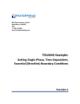
403 Poyntz Avenue, Suite B
Manhattan, KS 66502
USA
+1.785.770.8511
www.thunderheadeng.com
TOUGH2 Example:
Time-Dependent Essential (Direchlet)
Boundary Conditions
PetraSim 5
Table of Contents
Acknowledgements........................................................................................................................... iv
Time-Dependent Essential (Direchlet) Boundary Conditions ................................................................1
Create a One Cell Model ........................................................................................................................... 1
Material for Temperature Boundary Condition ........................................................................................ 1
Define Temperature Boundary Condition in Thin Cell.............................................................................. 2
Heat Flow into Boundary Condition Cell ................................................................................................... 3
Edit Solution Controls ............................................................................................................................... 5
Edit Output Controls ................................................................................................................................. 5
Save and Run............................................................................................................................................. 5
View Time History Plots ............................................................................................................................ 5
Boundary Condition using Thin Cell .......................................................................................................... 7
Boundary Condition using Thin Cell and Polygonal Mesh ........................................................................ 8
References....................................................................................................................................... 11
ii
Disclaimer
Thunderhead Engineering makes no warranty, expressed or implied, to users of PetraSim, and accepts
no responsibility for its use. Users of PetraSim assume sole responsibility under Federal law for
determining the appropriateness of its use in any particular application; for any conclusions drawn from
the results of its use; and for any actions taken or not taken as a result of analyses performed using
these tools.
Users are warned that PetraSim is intended for use only by those competent in the field of multi-phase,
multi-component fluid flow in porous and fractured media. PetraSim is intended only to supplement the
informed judgment of the qualified user. The software package is a computer model that may or may
not have predictive capability when applied to a specific set of factual circumstances. Lack of accurate
predictions by the model could lead to erroneous conclusions. All results should be evaluated by an
informed user.
Throughout this document, the mention of computer hardware or commercial software does not
constitute endorsement by Thunderhead Engineering, nor does it indicate that the products are
necessarily those best suited for the intended purpose.
iii
Acknowledgements
We thank Karsten Pruess, Tianfu Xu, George Moridis, Michael Kowalsky, Curt Oldenburg, and Stefan
Finsterle in the Earth Sciences Division of Lawrence Berkeley National Laboratory for their gracious
responses to our many questions. We also thank Ron Falta at Clemson University and Alfredo Battistelli
at Aquater S.p.A., Italy, for their help with T2VOC and TMVOC. Without TOUGH2, T2VOC, TOUGHREACT,
and TOUGH-Fx/HYDRATE, PetraSim would not exist.
In preparing this manual, we have liberally used descriptions from the user manuals for the TOUGH
family of codes. Links to download the TOUGH manuals are given at http://www.petrasim.com. More
information about the TOUGH family of codes can be found at: http://www-esd.lbl.gov/TOUGH2/.
Printed copies of the user manuals may be obtained from Karsten Pruess at <[email protected]>.
The original development of PetraSim was funded by a Small Business Innovative Research grant from
the U.S. Department of Energy. Additional funding was provided by a private consortium for the
TOUGHREACT version and by the U.S. Department of Energy NETL for the TOUGH-Fx/HYDRATE version.
We most sincerely thank our users for their feedback and support.
iv
Time-Dependent Essential (Direchlet) Boundary
Conditions
In this example we demonstrate how to apply time-dependent boundary conditions. The user should
refer to the PetraSim manual for further discussion. In this example, we will first illustrate the basic
concepts using a single cell model. We will add boundary condition cells to define boundary conditions
on the model cell. We will then demonstrate how to apply time-dependent boundary conditions to a
more complex model.
Create a One Cell Model
Following the instructions already presented in previous example problems, make a new model using
EOS1 and dimensions of 10x10x10 meters.
1.
2.
3.
4.
Edit the default layer to have only one cell in the Z-direction.
Create a 1 x 1 regular mesh.
Use the default material properties for the model.
The initial conditions for the model should be a temperature of 100 ˚C and a pressure of 1.0E6
Pa (single phase liquid).
5. Print time history data for the model cell
The single cell model is shown below. In the following description, “model” cell means this 10x10x10
cell. We add cells to define the boundary conditions. These will be called “boundary condition” cells.
Figure 1: Single cell model
Material for Temperature Boundary Condition
For the temperature boundary condition cell, we do not want flow into or out of the cell. This can be
accomplished by making a special material that has zero permeability and small porosity.
1
To make a new material to use in applying the temperature boundary conditions:
1.
2.
3.
4.
On the Properties menu, click Edit Materials...
In the Material Data dialog, click New
In the Name box, type TEMP
Click OK to create the new material, by default, the new material data will be based on
theROCK1 data
5. For the TEMP material, change the value in the Porosity box to 0.001. The cell will be essentially
all solid, so we can use the solid properties for our heat capacity calculations and neglect the
heat capacity of the small amount of fluid in the cell.
6. For the TEMP material, in all three Permeability boxes (X, Y, and Z), type 0.0. There will be no
flow into the cell.
Click OK to save changes and exit the Edit Materials dialog.
Define Temperature Boundary Condition in Thin Cell
To modify the thin cell so that it defines a temperature boundary condition:
1.
2.
3.
4.
Spin the model and click on the top. This should select only the thin cell.
Right-click and select Edit Cells…
In the Cell Name box, type TempBC
In the Vol. Factor box, type 1.0E20 (the volume of the cell will be the actual volume, 1, time the
factor, for a volume of 1.0E20 m3.
5. In the Material list, select TEMP (we want to use the special boundary condition material)
We will return to define sources /sinks in the extra cell. We use the default initial conditions in the
boundary condition cell. To turn on detailed printing of time history data:
1. Click the Print Options tab
2. Click to select both print options.
To define the connection between the boundary condition cell and the model cell:
1. Click the Connected Cells tab
2. In the ’To’ Cell box, type 1 (this boundary condition cell will be connected to the model cell with
ID 1)
3. In the Orientati… box, type 1 (use the TEMP material X permeability value for this connection)
4. In the Dist. ‘This’ box, type 0.001 (the flow distance in this boundary cell is small so that the
temperature boundary condition is applied to the surface of the model cell)
5. In the Dist. ‘To’ box, type 5.0 (the true distance of flow in the model cell)
6. In the Area box, type 100 (the true area between the cells)
7. In the Gravitati… box, type 1 (the boundary cell is directly above the model cell)
8. In the Rad. He… box, type 0.0 (no radiation heat transfer)
2
Click OK to save changes and exit the Edit Cell Data dialog.
Heat Flow into Boundary Condition Cell
We have now created a boundary condition cell that has a volume of 1.0E20 m3, a density of 2600
kg/m3, a porosity of 0.001, and a specific heat of 1000 J/kg-C. For this example, we will specify a
sinusoidal temperature history with an average of 100 ˚C, a amplitude of 50 ˚C, and a period of 30 days,
Figure 2.
Figure 2: Desired boundary condition temperature history
We calculate the heat flux as follows:
̇
where ̇ is the heat flow, is the cell volume, is the rock density, is the rock heat capacity,
is
the change in temperature, and is the change in time. Note that since the porosity is very small, we
only use the rock properties and apply this to the entire cell volume. The calculated heat flows to obtain
the desired temperature time history are shown in Table 1.
3
Table 1: Calculated heat flow to change boundary cell to desired temperature
Time
Day
0
1
2
3
4
5
6
7
8
9
10
11
12
13
14
15
16
17
18
19
20
21
22
23
24
25
26
27
28
29
30
Sec
0
86400
172800
259200
345600
432000
518400
604800
691200
777600
864000
950400
1036800
1123200
1209600
1296000
1382400
1468800
1555200
1641600
1728000
1814400
1900800
1987200
2073600
2160000
2246400
2332800
2419200
2505600
2592000
Temp
(C)
100
110.3956
120.3368
129.3893
137.1572
143.3013
147.5528
149.7261
149.7261
147.5528
143.3013
137.1572
129.3893
120.3368
110.3956
100
89.60442
79.66317
70.61074
62.84276
56.69873
52.44717
50.27391
50.27391
52.44717
56.69873
62.84276
70.61074
79.66317
89.60442
100
Heat Flow
3.12830090E+22
2.99157914E+22
2.72411102E+22
2.33758617E+22
1.84889759E+22
1.27940331E+22
6.53992972E+21
0.00000000E+00
-6.53992972E+21
-1.27940331E+22
-1.84889759E+22
-2.33758617E+22
-2.72411102E+22
-2.99157914E+22
-3.12830090E+22
-3.12830090E+22
-2.99157914E+22
-2.72411102E+22
-2.33758617E+22
-1.84889759E+22
-1.27940331E+22
-6.53992972E+21
0.00000000E+00
6.53992972E+21
1.27940331E+22
1.84889759E+22
2.33758617E+22
2.72411102E+22
2.99157914E+22
3.12830090E+22
1.00308642E+22
To specify this heat flow into the boundary cell:
1.
2.
3.
4.
5.
6.
In the tree display, expand the ExtraCells list and double-click the TempBC cell
Click the Sources/Sinks tab
Click Heat In
In the options list, select Table
Click the Edit button and type (or paste) the values shown Table 1
Click OK to save changes and exit the Heat Rates dialog
Click OK to save changes and exit the Edit Cell Data dialog.
4
Edit Solution Controls
Parameters relating to the solver and time stepping can be found in the Solution Controls dialog.
To specify the simulation end time:
1.
2.
3.
4.
5.
On the Analysis menu, click Solution Controls
In the End Time list, click User Defined and type 30 days
In the Max Time Step list, click User Defined and type 1 days
Click the Weighting tab
For Permeability at Interface list, click Harmonic Weighted (see the PetraSim user manual and
the TOUGH2 user manual for a supporting discussion)
6. Click the Options tab
7. For Boundary condition Interpolation, click Rigorous Step
8. Click OK
Edit Output Controls
By default, the simulation will print output every 100 time steps. For this simulation, we will specify
output every time step.
To specify the output frequency:
1. On the Analysis menu, click Output Controls
2. In the Print and Plot Every # Steps box, type 1
3. Click OK
Save and Run
The input is complete and you can run the simulation.
View Time History Plots
To view time history plots:
1.
2.
3.
4.
5.
On the PetraSim Results menu, click Cell History Plots
In the Variable list, click T (deg C)
In the Cell Name list, click TempBC
In the Cell Time History window, on the File menu, click Export Data… and save the data.
You can then import the data and compare the calculated boundary condition temperatures to
the desired values, as shown in Figure 3.
6. In the Cell Name list, click Model to view the time history of the temperature in the model cell.
This response shows a temperature change from 100 ˚C to a maximum of 100.5983 ˚C, Figure 4.
A hand calculation gives an analytic value of 100.597 ˚C.
5
Figure 3: Comparison of calculated and desired boundary condition cell temperatures
Figure 4: Time history response of model cell
When finished, you can close the Cell History dialog.
6
Boundary Condition using Thin Cell
We now repeat the specifying a temperature boundary condition, but using a thin cell instead of adding
an extra cell.
1. Open the previous model
2. Delete the extra cell
3. Save the model under a different name.
To define the thin cell:
1.
2.
3.
4.
5.
6.
In the Tree View, expand the Layers node and click Default
On the Edit menu, click Properties...
In Dz click Custom
In the first row Fraction box type 0.999 and in the Cells box type 1 (Figure 5)
In the second row Fraction box type 0.001 and in the Cells box type 1 (Figure 5)
Click OK to save changes to the default layer
Figure 5: Input of cell sizes
If you close and reopen the Edit Layers dialog, you will notice that Dz has been changed to a Regular
mesh with a Factor of 1.001E-03. This is an alternate way to describe the same sizes for two elements.
We now need to regenerate the mesh:
1.
2.
3.
4.
On the Model menu, click Create Mesh
For Mesh Type, select Regular
In the X Cells box, type 1
In the Y Cells box, type 1
7
5. Click OK to create the mesh
To set the boundary conditions in the thin top cell:
1.
2.
3.
4.
5.
6.
Spin the model and click on the top cell.
On the Edit menu, click Properties...
In the Cell Name box, type TempBC
In the Vol. Factor box, type 1.0E20 (this factor multiplies the geometric cell volume of 1 m3)
In the Material list, select TEMP (we want to use the special boundary condition material)
Click the Sources/Sinks tab, Click Heat In, and input the same values as described in the
previous Heat Flow into Boundary Condition Cell section.
7. Click the Print Options tab and select both print options
8. Click OK
Select the model cell, name it, and select the print options.
Run the analysis and essentially the same results will be obtained.
Boundary Condition using Thin Cell and Polygonal Mesh
We now repeat the specifying a temperature boundary condition, but using a polygonal mesh.
1. Open the previous model
2. Save the model under a different name.
We have already defined the spacing for the thin cell, so that does not need to be modified.
To regenerate the mesh:
1. On the Model menu, click Create Mesh
2. For Mesh Type, select Polygonal
3. Click OK to create the mesh
To calculate and set the boundary conditions in the top lower left polygonal cell:
1. Spin the model and click on the top cell in the lower left corner top layer cell, Figure 6. Note that
the projected area is 0.4217 m2 and that the volume is 4.2169E-3 m3 .
2. On the Edit menu, click Properties...
3. In the Cell Name box, type TempBC
4. In the Vol. Factor box, type 237.137E20 (this factor was chosen to give the cell a volume of
1.0E20 m3, the same value as in the previous examples)
5. In the Material list, select TEMP (we want to use the special boundary condition material)
6. Click the Sources/Sinks tab
7. Click Heat In
8. In the options list, select Table Flux and input the values shown in Table 2. These values were
calculated to give the same heat flow as in the previous examples, but use an area of 0.4217 m2.
8
9. Click the Print Options tab and select both print options
10. Click OK
We now repeat this for all top cells:
1. Spin the model, click the Select Mesh Layer tool, and click on the top cell in the lower left
corner. This will select the entire top layer .
2. Right-click and select Edit Cells…
3. In the Vol. Factor box, type 237.137E20
4. In the Material list, select TEMP (we want to use the special boundary condition material)
5. Click the Sources/Sinks tab
6. Click Heat In
7. In the options list, select Table Flux and input the values shown in Table 2.
8. Click OK
Figure 6: Selection of lower left cell in thin top layer
9
Table 2: Specification of heat flow using flux
Time
0
86400
172800
259200
345600
432000
518400
604800
691200
777600
864000
950400
1036800
1123200
1209600
1296000
1382400
1468800
1555200
1641600
1728000
1814400
1900800
1987200
2073600
2160000
2246400
2332800
2419200
2505600
2592000
Flux
7.41830900E+22
7.09409330E+22
6.45983168E+22
5.54324442E+22
4.38439078E+22
3.03391822E+22
1.55084888E+22
0.00000000E+00
-1.55084888E+22
-3.03391822E+22
-4.38439078E+22
-5.54324442E+22
-6.45983168E+22
-7.09409330E+22
-7.41830900E+22
-7.41830900E+22
-7.09409330E+22
-6.45983168E+22
-5.54324442E+22
-4.38439078E+22
-3.03391822E+22
-1.55084888E+22
0.00000000E+00
1.55084888E+22
3.03391822E+22
4.38439078E+22
5.54324442E+22
6.45983168E+22
7.09409330E+22
7.41830900E+22
2.37867304E+22
Select the at least two model cells, name them, and select the print options.
Run the analysis and essentially the same results will be obtained in the model cells.
Summary
This has illustrated how to apply temperature-only boundary conditions in a PetraSim/TOUGH2 model.
Other combinations of boundary conditions are discussed in the PetraSim User Manual. The principles
are the same.
10
References
1. Pruess, Karsten, Oldenburg, Curt and Moridis, George. TOUGH2 User's Guide, Version 2.0. Berkeley,
CA, USA : Earth Sciences Division, Lawrence Berkeley National Laboratory, November 1999. LBNL-43134.
2. Falta, Ronald, et al., et al. T2VOC User's Guide. Berkeley, CA, USA : Earth Sciences Division, Lawrence
Berkeley National Laboratory, March 1995. LBNL-36400.
3. Pruess, Karsten. Personal communication. 2003. email.
11