Download using the petrasim pre - Stanford School of Earth, Energy

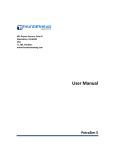
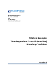
PROCEEDINGS, Twenty-Seventh Workshop on Geothermal Reservoir Engineering
Stanford University, Stanford, California, January 28-30, 2002
SGP-TR-171
USING THE PETRASIM PRE- AND POST-PROCESSOR FOR TOUGH2, TETRAD, AND STAR
Daniel Swenson1, Brian Hardeman1, Steve Butler2, Casey Persson1, and Charlie Thornton1
1
Thunderhead Engineering Consultants, Inc.
1006 Poyntz Ave., Manhattan, KS, 66502-5459, www.thunderheadeng.com
2
GeothermEx, Inc.
5221 Central Ave., Suite 201, Richmond, CA 94804-5829
ABSTRACT
PetraSim is a new interactive, cross-platform, preand post-processor that can be used to create reservoir models and display simulation results through
time. It provides the analyst a tool to rapidly develop
models and create the input files needed for the existing TOUGH2, TETRAD, and STAR simulation
programs. Key design decisions used in the development of PetraSim include: (1) high level geometric
feature definition of the model to allow relative independence from any particular simulator, (2) use of
Java for the graphical user interface to allow crossplatform execution, (3) automatic writing of the appropriate simulator input file, and (4) translation of
the simulator output files to a common visualization
format that is used for integrated 3D and time history
display.
MOTIVATION
A significant hurdle for new users of a reservoir
simulator is developing the infrastructure to create
valid meshes, select the appropriate solution controls,
and display results. Possible simulator options are
often activated by flags that are confusing and may
appear in unrelated locations in the text-based input
file. It is hard enough to solve nonisothermal, multicomponent, multiphase problems without the additional difficulty of preparing complex and lengthy
input files. While experienced users will have
learned the idiosyncrasies of their favorite simulator
and will have gathered their own toolkit for its use,
even they may need additional help to exploit models
with tens of thousands of cells or to enable rapid
remeshing for convergence studies.
The solution to this problem has four key features:
(1) use of a high level model description based on
geometric features of the reservoir (stratigraphy, well
coordinates), (2) presentation of the required input
options grouped in a logical format with appropriate
default options activated, (3) automatic writing of the
simulator input file in the correct format, and (4)
rapid access to visualization of results. Such a pro-
gram should be interactive, with immediate visual
confirmation of any user actions.
PetraSim is a new pre- and post-processor for
TOUGH2 (Pruess, 1999), TETRAD (ADA, 2000),
and STAR (Garg, 2001) that incorporates these features into an integrated program for model creation
and results display. In the remainder of this paper,
we describe the most significant features of PetraSim
and give an example of its use.
PETRASIM FEATURES
Problem Description/Conceptual Model
A significant difference between PetraSim and the
input file to a simulator is that PetraSim uses a geometric model to store the problem description rather
than a grid-based description. A geometric model is
a high-level, geometry-based representation of an
object. This representation provides a natural and
convenient location to store all of the necessary information associated with a numerical analysis problem, such as material properties and boundary conditions. Combining the geometric model with the parameters of the analysis creates a problem description
unique to the problem at hand, but independent of
any given analysis method. Conceptually, this also
means that the same model description can be used
for different simulators.
The advantage of such an approach is clear. When
the grid serves as the fundamental carrier of information, any change in geometry, material properties, or
initial conditions requires identification of the associated cells and a change to their properties. Refinement of a mesh may require the user to essentially
start the analysis over from the beginning, redefining
all associated cell conditions.
In contrast, if a high level geometric description is
used, the grid may be changed at will and all properties and boundary conditions will automatically be
applied when the simulator input file is written. As a
particular example, in PetraSim a well is defined by
its trajectory, open interval, and associated flow rates
or pressures. This description is independent of the
mesh. Obviously, at some point the well must be
associated with the particular cells of a grid, but this
is handled automatically when the simulator input file
is written. Before then, the user can change the mesh
at will and PetraSim will correctly identify the cells
intersected by the well trajectory. Figure 1 shows a
simple model in which there are three wells and material boundaries that separate the reservoir into regions. Material properties and boundary conditions
can be applied to this model even though a grid has
not yet been defined.
cial element to define the confining bed material
properties. Finally, each element of the fracture must
have its contact area with the confining bed defined
as input. Undoubtedly there are historical reasons
why the input file is organized in such a way.
Figure 1: Simple model with wells and material
boundaries that define regions
Figure 2: Dialog used to specify TOUGH2 confining bed data
Figure 1 also illustrates several options for high level
interaction with the model. On the left of the window
is a tree that displays features in the model. Using
the tree, the user can select a specific feature. Alternately, the model can be manipulated in the 3D display and features selected with the mouse. In either
case, once a feature is selected all associated properties can be modified. As illustrated, the top region of
the model (highlighted in yellow) has been selected
so that a new material can be assigned to the region.
When the grid is created, all cells in that region will
inherit the region material data.
Two other examples of organizing data will be illustrated. The first is the definition of material properties in TOUGH2. Figure 3 shows the dialog used to
input this data. The left pane allows the user to select
any existing material or create a new one. In the
right pane, the user can edit properties of the selected
material. This includes MINC data (only activated if
the MINC option has been enabled) and, under the
Advanced button, the capability to customize relative
permeability and capillary functions.
The user interface, however, can be much simpler.
Figure 2 shows how the required information is presented in PetraSim. A box is checked to indicate that
this boundary condition is active, then initial temperature and material properties are specified, with
reasonable default values given. When the TOUGH2
input file is written, PetraSim handles the details of
creating the artificial element, specifying the contact
areas, etc. As a result, there is a much greater chance
that the user will actually solve the problem as intended.
User Input
A properly designed user interface can guide the user
through the model definition process, organizing into
logical groupings input that may appear in many locations in a simulator input file. The interface can
ease learning for a beginning user and act as a reminder for an experienced user.
As an example, the TOUGH2 code has the capability
to model a fracture bounded by a confining bed that
only conducts heat. To activate this option, the user
must activate the MOP(15) flag, insert an artificial
element at the end of the ELEME data, ensure that it
is initialized to the confining bed initial conditions,
and insert a material that is referenced by the artifi-
Figure 3: TOUGH2 material definition
The TETRAD material dialog is similar to that in
Figure 3, but, since TETRAD allows property data to
vary for every cell, PetraSim allows global property
definitions as functions or contours for which the
data is then calculated for each cell.
Figure 4 illustrates the organization of the solution
parameters of TOUGH2. Again, common parameters
have been grouped in an arrangement that helps the
user understand and specify all parameters from one
location. Similar organization is used for the solver
and other solution parameters.
Figure 5: Prismatic grid defined on model
In the future, more general grids will be developed
for TOUGH2, since it uses the integral finite difference method. However, for convergence to the correct solution, the integral finite difference method
requires that the mesh satisfy the Voronoï condition
(that is, boundaries of the elements must be formed
by planes which perpendicularly bisect the lines between volume centers). Generation of such grids is
relatively simple in 2D, but algorithms are much
more complex for a general 3D Voronoï grid.
Figure 4: Solution controls dialog
Gridlines can be edited, deleted, or inserted interactively. Figure 6 shows an example of a grid in which
the grid has been edited to be more refined in the
center. This editing is performed in the Grid Editor
window.
Grid Definition
An appropriate grid for an analysis must satisfy several constraints: (1) it must be able to capture the
essential features of the reservoir, such as stratigraphic layers with different material properties, (2)
it must be sufficiently refined to accurately represent
regions of high gradient in the solution, and (3) it
must satisfy the requirements of the simulator. The
simplest grid to construct and that will satisfy all
simulator requirements is a prismatic 3D grid. At the
time of this paper, a 3D prismatic grid and a matching radial RZ grid are the two grid types supported
for TOUGH2. TETRAD has the additional capability to allow different elevations and thicknesses for
each cell.
The grid is created by specifying the number of divisions in each direction. Figure 5 illustrates a simple
grid. There is no limitation on grid size, and, as will
be discussed, the grid can be locally refined and
modified using disabled elements so that stratigraphy
and non-uniform elevations can be adequately represented even using a uniform grid.
Figure 6: Example of non-uniform grid
It is important to remember that the model has a grid,
but the grid is not the model. The model is a higher
level, grid independent, description of the reservoir.
Editing of Cell Properties
After the grid is defined, cell properties may be edited directly. The goal of PetraSim is not to encourage cell editing. However, during the transition from
legacy models, and until features of every simulator
can be implemented at a high level, there may be
times when individual cell editing is required. This is
accomplished in the Grid Editor window, which allows the user to select a grid layer and edit any cell in
that layer, Figure 7.
Writing a Simulator Input File
The whole point of a pre-processor is to automatically write the simulator input file in a correct format
and without intervention by the user. In PetraSim,
this task is performed by a function that accesses the
model, the grid, and all other data necessary to write
the file.
A portion of an example file is shown in Figure 9.
Since the TOUGH2 program has not been modified,
the input file written by PetraSim is in standard
TOUGH2 format. Since the computer is writing the
file, there is no need to keep the file small. Each
element, connection, and initial condition is written
explicitly. It can also be seen that the elements are
given sequential numerical names. It is intended that
the user never need to know or examine these names.
Any type of data, such as the definition of a source or
sink, knows the associated cell and correctly writes
the cell name when the simulator input file is written.
Figure 7: Grid editor
In the Grid Editor the user can display any editable
value and then select a cell or group of cells to edit
that value. The user can also select cells to define
sources and sinks, Figure 8. Again, the preferred
approach is to define a high level well, but if desired,
the user has control at the cell level.
Figure 9: Portion of TOUGH2 input file created
by PetraSim
Solution
The eventual goal is to integrate simulator execution
into PetraSim. At the present time, the user can keep
the PetraSim window open, but needs to execute the
analysis separately in the standard way. When the
solution is complete, the user may post-process the
results.
Figure 8: Defining a source or sink in the Grid
Editor
Visualization
After the solution is completed, either 3D or time
history plots of the results may be made. Figure 10
shows an example of an iso-surface plot of temperature from a TETRAD analysis. PetraSim uses a
common results display component for all simulators,
with different translators to read the data from the
simulator-specific results files. For TOUGH2, the
standard printed output file is parsed to extract the
cell data. For TETRAD, the GridView format file is
read.
As shown in Figure 10, once the data is read, the user
can select any available variable and time for plotting. The user can rotate, pan, and zoom the image
interactively. Image details, such as the number of
iso-surfaces and the data range can be controlled.
Also, cutting planes can be defined on which the results are contoured. Finally, the user can export the
data in a simple X, Y, Z, value format for import into
other presentation quality graphics programs, such as
TECPLOT. In PetraSim, results are readily accessible to rapidly evaluate the analysis.
TETRAD, the time history results are read in FPLOT
format and for TOUGH2, the FOFT file is read.
As illustrated in Figure 11, the user can select any
saved data and make a time history plot. If a cell was
given a user-defined name, this name will be available for selecting the plot data. Once any plot is
made, the data can be exported in a format that can
be read in a spreadsheet or other presentation quality
graphics program.
EXAMPLE
To demonstrate PetraSim features, we give instructions to solve a variation on Problem 4 – Five-spot
Geothermal Production/Injection (EOS1) described
in the TOUGH2 User’s Manual (Pruess et al., 1999).
This problem models a five-spot pattern of injection
and production from a geothermal reservoir.
The geometry of the problem is shown in Figure 12.
Water is injected in the center well and produced at
the four corner wells. We use a half-symmetry
model.
Depth=305 m
Injection
Grid
21x11x6
Production
Figure 10: Iso-surface plot of temperatures (from
TETRAD GridView data file)
In a similar manner, time history plots of results may
be made, Figure 11.
L=1000 m
Figure 12: Five-spot well pattern with grid modeling 1/2 symmetry domain
Model Creation
Start PetraSim by selecting Start/Programs/PetraSim.
To define the boundary of the model, select
Model/Define Boundary… and create the model
boundary with the values X min = -500, X max =
500., Y min = 0.0, Y max = 500., Z min = -305., and
Z max = 0.0. We create the grid on the model by
selecting Model/Create Grid… and specifying 21 X
divisions, 11 Y divisions, and 6 Z divisions. The
resulting mesh is displayed in Figure 13.
Figure 11: Time history plot (from TOUGH2
FOFT file)
Similar to the 3D plots, a common time history display component is used, with different translators to
read the different simulator results files.
For
Solution Controls
We next specify the information that will control the
solution by selecting Properties/Solution Controls… .
The Times tab allows us to specify parameters associated with the start and ending of the analysis and
the time steps used for the calculation. In this case,
we will start at 0 sec, end at 1.5E9 sec (approximately 50 years), and specify an initial time step size
of 100 sec. We allow a maximum of 200 time steps
and select the Automatic Time Step adjustment option.
J/kg-C. We need to specify both the relative permeability data and the capillary pressure data. To do
this, select Advanced and then the appropriate tabbed
pane. Use Corey’s Curves for the relative permeability, with constants of 0.30 and 0.05 and use a
Linear Function for the capillary pressure with constants of 0.0, 1.0, and 0.0.
Initial Conditions
To specify the default initial conditions, select Properties/Initial Conditions…. Select the Two-Phase (T,
Sg) option and then specify the temperature to be 300
C and the gas saturation to be 0.01.
Figure 13: Five spot model after creating the grid
We will change the solver to the stabilized biconjugate gradient solver by selecting the Solver tab,
then selecting that solver, Figure 14.
Sources and Sinks
Sources and sinks are defined by selecting cells individually in the Grid Editor. Select Model/Edit Grid
to display the Grid Editor. There are a total of 6 layers in the Z direction. We will inject in layer 5 (the
second from the top). To define the injection, first
click on the layer spin-box on the tool bar to layer 5.
Then, right click on the center lower cell and select
the Source/Sink… menu option. Select the Injection:
Water/Steam option with a flow rate of 15.0 kg/s and
an enthalpy of 5.0E5 J/kg. We will produce from
layer 3, so click on the layer spin-box arrow until
layer 3 is selected. Next, right click on the top right
cell and select the Source/Sink… menu option. Select
Production Mass Out, then specify the mass flow rate
at 7.5 kg/s, Figure 14. Repeat this for the top left
cell. At this point, we have defined one injection cell
and two production cells.
Write PetraSim and TOUGH2 Files
We have now completed the input necessary for the
solution. First save the PetraSim file by selecting
File/Save… and save the file with the name
3d_five_spot.sim (the .sim extension will be added
automatically if you do not give it).
We will also save a TOUGH2 input file by selecting
File/Write TOUGH2 File… and giving the name
3d_five_spot.dat (the .dat extension will be automatically added if not specified).
Figure 14: Selecting the solver
Perform TOUGH2 Analysis
At the present time, TOUGH2 execution is planned
from within PetraSim. At present, the user must
manually execute the TOUGH2 analysis. Typically
this will be done in a command window.
Material Properties
To define the material properties, select Properties/Materials… . Change the material name to
POMED, the rock density to 2650 kg/m3, the porosity to 0.01, the permeabilities to 6.0E-15 m2, the conductivity to 2.1 W/m-C, and the specific heat to 1000
View Results of the Analysis
Results can be displayed using 3D iso-surfaces, as
contours on 3D planes, or as time history plots at the
cells selected by the user for time history output.
Data for the 3D views are obtained from the output
file (in this case 3d_five_spot.out). Data for time
history plotting is obtained from the FOFT file.
To view the results in 3D, select Results/3D Contours… . This will display a window in which the
user can select the display variable, the time, and
options on the number of isosurfaces, the grid, the
plot range, and slicing planes. Figure 15 shows a plot
of temperature at 1.5E9 sec. This view shows the
grid and uses two slice planes on which matching
contours are drawn.
STATUS AND ACCESS
Development of PetraSim is continuing, with a first
commercial release scheduled for mid-2002. However, sufficient capability has been implemented for
PetraSim to be a useful tool and an early access release is available. Implementation is most complete
for the TOUGH2 version, with nearly all TOUGH2
capability accessible through the interface. The
TETRAD version includes grid editing, 3D visualization, and time history plotting. The STAR version
has not yet been completed, but should progress rapidly using the foundation already completed. The
early access release can be downloaded at
www.thunderheadeng.com under the software section.
ACKNOWLEDGEMENTS
Figure 15: Display of calculated temperatures at
t=1.5E9 sec
To view time history plots of cell data, select Results/Cell Results…, Figure 16. In this window the
user can select the plot parameter and the cell for
which results are to be plotted. This plotted data can
be written in column format to a file by selecting
File/Export Data… in the time history menu. This
data can then be imported into another program for
additional plotting or comparison with data.
We are grateful for the feedback provided by users of
the early access release, including: Kit Bloomfield,
Jochen Bundschuh, Paul Spielman, John McCray,
and Thomas Beuth. We thank Karsten Pruess,
Anthony Au, and Sabodh Garg for help with the
respective simlators. This development is a joint
venture between Thunderhead Engineering and
GeothermEx, with primary funding from a Department of Energy Phase II Small Business Innovative
Research grant.
REFERENCES
ADA International Consulting, “TETRAD 2000 User
Manual,” 705 Hawkwood Blvd., N. W., Calgary,
Alberta, Canada T3G 2V7, Tel. (403)630-3872,
2000.
Garg, Sabodh, SAIC, 10260 Campus Point Drive,
Mail Stop X1133, San Diego, CA 92121, 2001.
Pruess, K., Oldenburg, C., and Moridis, G.,
TOUGH2 User’s Guide, Version 2.0, Earth Sciences
Division, Lawrence Berkeley National Laboratory,
LBNL-43134, November, 1999.
Figure 16: Cell results