Download Production from a Geothermal Reservoir (EWASG)

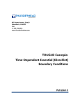
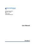
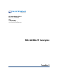
403 Poyntz Avenue, Suite B
Manhattan, KS 66502
USA
+1.785.770.8511
www.thunderheadeng.com
TOUGH2 Example:
Production from a Geothermal
Reservoir (EWASG)
PetraSim 5
Table of Contents
Acknowledgements........................................................................................................................... iv
Production from a Geothermal Reservoir (EWASG) .............................................................................1
Description ................................................................................................................................................ 1
Create an EWASG Model .......................................................................................................................... 1
Specify the Solution Mesh ........................................................................................................................ 1
Specify Z Divisions ................................................................................................................................. 1
Create the Mesh ................................................................................................................................... 2
Global Properties ...................................................................................................................................... 2
Material Properties ................................................................................................................................... 3
Initial Conditions ....................................................................................................................................... 4
Define Reservoir Production ..................................................................................................................... 4
Solution Controls....................................................................................................................................... 5
Output Controls ........................................................................................................................................ 5
Save and Run............................................................................................................................................. 5
View 3D Results......................................................................................................................................... 6
View Cell History Plots .............................................................................................................................. 7
Line Plots ................................................................................................................................................... 8
References....................................................................................................................................... 10
ii
Disclaimer
Thunderhead Engineering makes no warranty, expressed or implied, to users of PetraSim, and accepts
no responsibility for its use. Users of PetraSim assume sole responsibility under Federal law for
determining the appropriateness of its use in any particular application; for any conclusions drawn from
the results of its use; and for any actions taken or not taken as a result of analyses performed using
these tools.
Users are warned that PetraSim is intended for use only by those competent in the field of multi-phase,
multi-component fluid flow in porous and fractured media. PetraSim is intended only to supplement the
informed judgment of the qualified user. The software package is a computer model that may or may
not have predictive capability when applied to a specific set of factual circumstances. Lack of accurate
predictions by the model could lead to erroneous conclusions. All results should be evaluated by an
informed user.
Throughout this document, the mention of computer hardware or commercial software does not
constitute endorsement by Thunderhead Engineering, nor does it indicate that the products are
necessarily those best suited for the intended purpose.
iii
Acknowledgements
We thank Karsten Pruess, Tianfu Xu, George Moridis, Michael Kowalsky, Curt Oldenburg, and Stefan
Finsterle in the Earth Sciences Division of Lawrence Berkeley National Laboratory for their gracious
responses to our many questions. We also thank Ron Falta at Clemson University and Alfredo Battistelli
at Aquater S.p.A., Italy, for their help with T2VOC and TMVOC. Without TOUGH2, T2VOC, TOUGHREACT,
and TOUGH-Fx/HYDRATE, PetraSim would not exist.
In preparing this manual, we have liberally used descriptions from the user manuals for the TOUGH
family of codes. Links to download the TOUGH manuals are given at http://www.petrasim.com. More
information about the TOUGH family of codes can be found at: http://www-esd.lbl.gov/TOUGH2/.
Printed copies of the user manuals may be obtained from Karsten Pruess at <[email protected]>.
The original development of PetraSim was funded by a Small Business Innovative Research grant from
the U.S. Department of Energy. Additional funding was provided by a private consortium for the
TOUGHREACT version and by the U.S. Department of Energy NETL for the TOUGH-Fx/HYDRATE version.
We most sincerely thank our users for their feedback and support.
iv
Production from a Geothermal Reservoir (EWASG)
Description
This example is Problem 12 - Production from a Geothermal Reservoir with Hypersaline Brine and CO2
(EWASG) described in the TOUGH2 User's Manual (1). This problem examines production from a
hypothetical geothermal reservoir with high salinity and CO2. Fluid withdrawal causes pressure to drop
near the production well. Boiling of reservoir fluid gives rise to dilution of CO2 in the gas phase and to
increased concentrations of dissolved NaCl, which begins to precipitate when the aqueous solubility
limit is reached. As the boiling front receded from the well, solid precipitate fills approximately 10% of
the original void space, causing permeability to decline to approximately 28% of its original value.
The mesh uses a 1D radial geometry.
Create an EWASG Model
We will first create a new model using the EWASG EOS.
From the File menu, select New… to open the New Model dialog.
1. For the Simulator Mode, choose TOUGH2.
2. For the Equation of State (EOS), choose EWASG.
3. For the Model Bounds, enter the values from Table 1.
Table 1: Model boundary dimensions
Axis
X
Y
Z
Min (m)
5.0
0.0
-500.0
Max (m)
1000.0
1.0
0.0
Click OK to close the New Model dialog and create the model.
Specify the Solution Mesh
The solution mesh must be specified in two steps. First the Z divisions must be specified per layer. Then
the mesh can be created using the Create Mesh dialog.
Specify Z Divisions
We must first specify one Z division for the default layer. To do so, we will open the Edit Layers dialog.
On the Model menu, select Edit Layers….
1.
2.
3.
4.
In the layers list in the left-hand pane, select the Default layer.
In the right-hand pane, select Regular for Dz.
In the Cells box, type 1.
In the Factor box, type 1.0.
1
Click OK to apply the changes and close the Edit Layers dialog.
Create the Mesh
We will now create the radial solution mesh using the Create Mesh dialog. To open the dialog, on the
Model menu, select Create Mesh….
1.
2.
3.
4.
For the Mesh Type, select Radial.
For the Divisions, select Regular.
In the Radial Cells box, type 100.
In the Factor box, type 1.03705.
Click OK to create the mesh.
We have selected Radial Mesh as the mesh type. This means that a 2D cylindrical RZ mesh will be
created in which X corresponds to cylindrical R, Z corresponds to cylindrical Z, and the Y coordinate
corresponds to cylindrical Theta (which is not used). 100 cells extend in the R direction, with an X Factor
of 1.03705. This means that each cell is 1.03705 times the size of the previous cell in the R direction.
These were chosen to give a first cell length of 2.0 m, which is the value used in the TOUGH2 example.
See the PetraSim User Manual for instructions on how to calculate the appropriate factor.
The resulting mesh is displayed in Figure 1. Click the Front View button
model until the front is visible.
on the toolbar or rotate the
Figure 1: The resulting model
Global Properties
Global properties are those properties that apply to the entire model. We will make changes to some of
the EOS options, including activating molecular diffusion. To edit global properties, you use the Global
Properties dialog.
2
On the Properties menu, click Global Properties… (or click
1.
2.
3.
4.
5.
6.
7.
8.
9.
10.
11.
12.
13.
on the main toolbar).
In the Global Properties dialog, select the Analysis tab.
In the Name box, type Geothermal Production, Brine and CO2.
In the Global Properties dialog, select the EOS tab.
Select Non-Isothermal.
In the Type of NCG list, select CO2.
For Dependence of Permeability on Pore Space, select Tubes in Series.
In the phi box, type 0.8.
In the G box, type 0.8.
In the Property Dependence on Salinity list, select Full Dependence.
In the Brine Enthalpy Correction list, select Michaelides.
Select the Include Vapor Pressure Lowering checkbox.
Do NOT select Molecular Diffusion.
Click OK to close the Global Properties dialog.
Material Properties
To specify the material properties, use the Material Data dialog.
1.
2.
3.
4.
5.
6.
7.
8.
On the Properties menu, click Edit Materials… (or click
on the toolbar).
In the Name box, type POMED.
In the Density box, type 2600.0.
In the Porosity box, type 0.05.
In all three Permeability boxes (X, Y, and Z), type 50e-15.
In the Wet Heat Conductivity box, type 2.0.
In the Specific Heat box, type 1000.0.
Click Apply to save the changes.
In addition to the physical rock parameters, we also need to specify the relative permeability and
capillary pressure functions for this material. These options can be found in the Additional Material
Data dialog. To open this dialog, click the Additional Material Data… button.
To specify the relative permeability function
1.
2.
3.
4.
Select the Relative Perm tab.
In the Relative Permeability list, select Corey’s Curves.
In the Slr box, type 0.3.
In the Sgr box, type 0.05.
The default capillary pressure (none) is correct for this example.
Click OK to exit the Advanced Material Data dialog.
Click OK again to save your settings and exit the Material Data dialog.
3
Initial Conditions
The initial state of each cell in the model must be defined. To specify global initial conditions that will be
used as the default for all cells in the model, on the Properties menu, click Initial Conditions... (or click
on the toolbar).
To set the initial conditions
1.
2.
3.
4.
5.
Select the Two Fluid Phases (P, Xsm, Sg, T) state option.
In the Pressure box, type 6.0E6.
In the Temperature box, type 275.55.
In the Gas Saturation box, type 0.45.
In the Salt Mass Fraction box, type 0.3.
Click OK to close the Default Initial Conditions dialog.
Define Reservoir Production
In this model, fluid is produced from the inner cell.
1. In the 3D View, click the Front View button
on the toolbar or rotate the model until the front
is visible.
2. Use the Zoom Box tool
to zoom in on the left side of the model until the left-most cell is
visible.
3. Using the 3D Orbit Navigation tool , right click the left-most cell and from the context menu,
select Edit Cells... as shown in Figure 2.
4. In the Cell Name box, type Production.
5. Click the Sources/Sinks tab.
6. In the Production section, select the Mass Out check box.
7. In the Rate box, type 65.
8. Click the Print Options tab.
9. Select the Print Time Dependent Flow and Generation (BC) Data.
10. Click OK to close the Edit Cell Data dialog.
4
Figure 2: The cell to be selected
Solution Controls
We will now define the solution control options.
1.
2.
3.
4.
5.
6.
On the Analysis menu, click Solution Controls… (or click
on the main toolbar).
In the End Time box, type 2.0E6 (approximately 23 days).
In the Time Step list, ensure that Single Value is selected.
In the Time Step box, type 1000. This is the initial time step.
Select Enable Automatic Time Step Adjustment.
Click OK to exit the Solution Controls dialog.
Output Controls
By default, the simulation will print output every 100 time steps. We can increase the frequency of the
output in the Output Controls dialog.
1.
2.
3.
4.
5.
6.
On the Analysis menu, click Output Controls… (or click
on the main toolbar).
In the Print and Plot Every # Steps box, type 10.
Next to the Additional Print & Plot Times, click the Edit… button.
In the Additional Print Times table, type .50E5. This will force a solution printout at this time.
Click OK to exit the Additional Print Times dialog.
Click OK to exit the Output Controls dialog.
Save and Run
The input is complete and you can run the simulation. If you haven’t already, you may want to save
your model in a new directory. For example
1. On the File menu, click Save (or click
on the main toolbar).
5
2. Create a new folder named ewasg_geothermal and in the File Name box, type geothermal.sim.
3. Click Save.
To run the simulation, on the Analysis menu, click Run TOUGH2 (or click
on the main toolbar).
During the solution, a graph will display the time step size.
View 3D Results
To view the 3D results for a simulation, on the Results menu, click 3D Results (or click
on the main
toolbar). The data for the current simulation will be automatically loaded and displayed.
To show gas saturation contours for the last time step
1. In the Time(s) list, select the last entry (2.0E6).
2. In the Scalar list, select SG.
3. Click to clear the Show Isosurfaces checkbox.
To add a slice plane on which contours will be displayed, click Slice Planes…. For this example we will
show one slice plane. To configure the slice plane
1.
2.
3.
4.
In the Axis list, select Y.
In the Coord box, type 0.5.
Select the Scalar check box.
Click Close.
To orient and view the model with mesh
1. Click the Front View button
on the toolbar or rotate the model until the front is visible.
2. On the View menu, click Show Mesh.
The view can be zoomed and panned by holding the Alt and Shift keys, respectively, and dragging the
mouse. After moving the view to the upper left corner of the model, the resulting contour plot is shown
in Figure 3.
6
Figure 3: 3D representation of the saturation of gas
Close the 3D Results window.
View Cell History Plots
You can view time history plots with the Cell History dialog. On the Results menu, click Cell History
Plots (or click
on the main toolbar).
The Cell History dialog will be displayed. In this window, you can display time history data using a
plotting parameter and a list of cells. For example, to view the gas saturation in the Heat Source cell
1. In the Variable list, select SG.
2. In the Cell Name list, select Production.
Figure 4 shows the time history plot of SG at the production cell. The user can export this data for
plotting in spreadsheets.
7
Figure 4: The cell history plot for gas saturation in the production cell
Close the Cell History window.
Line Plots
PetraSim also supports line plots, where you define a line in 3D space and the data is interpolated along
the line. To make a line plot
1. First open the 3D results view. On the Results menu, click 3D Results (or click
on the main
toolbar).
2. On the File menu, click Line Plot….
3. In the Point 1 coordinate boxes (X, Y, and Z) type 5.0, 0.5, and -250.0, respectively.
4. In the Point 2 coordinate boxes (X, Y, and Z) type 1000.0, 0.5, and -250.0.
5. Click OK to close the Line Plot dialog.
6. This will open a Line Plot window.
7. In the Variable list, select P (Pa).
8. In the Time list, select 2.0E06 (the last time).
The plot is shown in Figure 5. You can export this data to a comma separated value file for import into a
spreadsheet.
8
Figure 5: Line plot of pressure
Close the Line Plot window.
Data saved using the line plot are shown in the same format as in the TOUGH2 user’s manual in Figure 6.
The calculated results compare well with the manual results.
Figure 6: Results for comparison with TOUGH2 manual
9
References
1. Pruess, Karsten, Oldenburg, Curt and Moridis, George. TOUGH2 User's Guide, Version 2.0. Berkeley,
CA, USA : Earth Sciences Division, Lawrence Berkeley National Laboratory, November 1999. LBNL-43134.
10