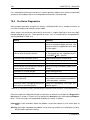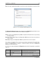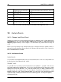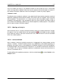
1
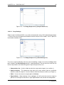
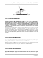
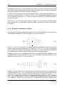
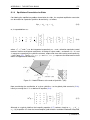
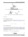
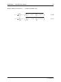
APPENDIX C. THEORETICAL BASIS C.1.3 171 Equilibrium Formulation for Slabs Considering the equilibrium problem formulation for slabs, the required equilibrium constraint can be written for a potential yield-line discontinuity i as follows: BTi ti + λfLi − qi = −fDi (C.5) or, in expanded form as: αi βi −βi αi 0 0 0 li 2 1 −αi −βi 0 li βi −αi 2 0 0 −1 mxA myA tzA mxB myB tzB mDni Mni mLni + λ mLti − Mti = − mDti fDi Si fLi (C.6) where mxj , myj and tzj can be interpreted respectively as x and y direction equivalent nodal moments and an out-of-plane nodal force, all acting at a given node j, and where Mni , Mti and Si represent respectively the yield-line moment, torque and shear force acting on discontinuity i (see Figure C.1). Finally, mDti , mDti , fDi and mLti , mLti , fLi represent the dead and live load effects as applied to discontinuity i. Figure C.1: Nodal moments at the ends of yield-line i (AB) Now considering the contribution of a given yield-line i to the global yield constraint (C.2c), initially assuming that Ni is as defined in equation (C.4): T Ni qi = 1 0 0 −1 0 0 0 1 0 0 −1 0 0 0 1 0 0 −1 Mni Mti ≤ S i mp+ i mp− i mp+ ti mp− ti sp+ i sp− i (C.7) Although at a typical yield-line the inequality equation (C.7) reduces simply to mp− ≤ Mni ≤ i mp+ , by inspection it is clear that more complex yield functions could be introduced if required, i c LimitState Ltd