Download Getting Started with LSE

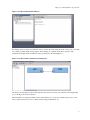
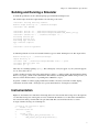
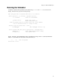
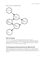
Getting Started with the Liberty
Simulation Environment
The Liberty Research Group
Getting Started with the Liberty Simulation Environment
by The Liberty Research Group
Version 1.0p1 Edition
Table of Contents
Preface......................................................................................................................................................................vi
Typographical conventions used in this book..................................................................................................vi
1. Installation ............................................................................................................................................................1
Getting the Liberty Simulation Environment ...................................................................................................1
Software Prerequisites ......................................................................................................................................1
Java..........................................................................................................................................................1
g++ ..........................................................................................................................................................1
Ant...........................................................................................................................................................2
Python .....................................................................................................................................................2
Perl ..........................................................................................................................................................2
GNU binutils...........................................................................................................................................2
Operating system notes.....................................................................................................................................3
Ubuntu Linux ..........................................................................................................................................3
Solaris 10 (SPARC) ................................................................................................................................3
Cygwin....................................................................................................................................................4
Installing the LSE Bundle ................................................................................................................................4
Installing Individual LSE Packages..................................................................................................................4
Preparing Your Environment ............................................................................................................................5
Getting help ......................................................................................................................................................5
2. A First Machine Specification .............................................................................................................................6
The Initial Specification ...................................................................................................................................6
Visualization .....................................................................................................................................................7
Building and Running a Simulator ...................................................................................................................8
Instrumentation.................................................................................................................................................9
Collecting Data .....................................................................................................................................10
Events....................................................................................................................................................11
Parameters and Userpoints .............................................................................................................................12
Full Specification............................................................................................................................................12
3. An LFSR Specification.......................................................................................................................................14
The Specification ............................................................................................................................................14
New Modules..................................................................................................................................................16
Multiports .......................................................................................................................................................16
Initial Values and Dynamic Identifiers ...........................................................................................................16
Initial Value...........................................................................................................................................17
Dynamic Identifiers...............................................................................................................................17
Examining the Output.....................................................................................................................................17
Running the simulator ....................................................................................................................................17
Control, Data, Enable, and Ack......................................................................................................................18
Control Points.................................................................................................................................................19
Input Control Points..............................................................................................................................20
Output Control Points ...........................................................................................................................20
Breaking the Loop.................................................................................................................................21
Full Code...............................................................................................................................................22
The xor_gate Module.....................................................................................................................................23
iii
4. LSE and Emulation............................................................................................................................................26
The Specification ............................................................................................................................................26
Setting up for Emulation ................................................................................................................................27
Overall Specification ......................................................................................................................................27
Emulating Instructions....................................................................................................................................28
Getting the Next PC........................................................................................................................................29
Creating New Dynamic Identifiers .................................................................................................................29
Running the Simulator....................................................................................................................................30
5. Module Writing ..................................................................................................................................................32
The Model of Computation ............................................................................................................................32
The Module Execution Life Cycle........................................................................................................32
Start of Timestep...................................................................................................................................33
The Heterogeneous Synchronous Reactive MoC and LSE ..................................................................33
End of timestep .....................................................................................................................................34
Modules ..........................................................................................................................................................34
Leaf Modules to Module Instances.......................................................................................................34
Module Functions .................................................................................................................................35
Handlers ................................................................................................................................................35
Declaring Leaf Modules .......................................................................................................................36
Automatic Generation of Skeletons ......................................................................................................36
A. Packages Included in the Liberty Simulation Environment .........................................................................38
scripts..............................................................................................................................................................38
ext_java...........................................................................................................................................................38
domains...........................................................................................................................................................38
lse....................................................................................................................................................................38
corelib .............................................................................................................................................................38
emulib .............................................................................................................................................................38
visualizer.........................................................................................................................................................38
iv
List of Figures
2-1. LSE Compilation Overview................................................................................................................................6
2-2. LSE Visualizer Initial Windows .........................................................................................................................7
2-3. LSE Visualizer Visualization of Example 2-1 ....................................................................................................8
3-1. A 3-bit LFSR ....................................................................................................................................................15
3-2. Visualization of Example 3-1 ...........................................................................................................................15
3-3. 3 wire control semantics in LSE .......................................................................................................................18
3-4. Combinational loop ..........................................................................................................................................19
3-5. Input Control Point ...........................................................................................................................................20
3-6. Output Control Point.........................................................................................................................................21
4-1. Visualization of the simple IA64 specification .................................................................................................27
5-1. The Cycle of Computation in LSE ...................................................................................................................32
v
Preface
This book provides an entry point into the Liberty Simulation Environment, guiding users through installation and
some primitive use of the system.
Typographical conventions used in this book
The following typefaces are used in this book:
•
Normal text
•
Emphasized text
• The name of a program variable
• The name of a constant
•
The name of an LSE module
•
The name of a package
•
The name of an domain class
• The name of an attribute in a domain description file
•
The name of an emulator
•
The name of an emulator capability
•
The name of a module parameter
•
The name of a module port
• Literal text
• Text the user replaces
• The name of a file
•
The name of an environment variable
•
The first occurrence of a term
vi
Chapter 1. Installation
This chapter will walk you through the setup and installation of the Liberty Simulation Environment. LSE
requires that you define a number of environment variables and install some packages that may not currently exist
on your machine. This section contains details on what must be done.
Getting the Liberty Simulation Environment
The Liberty Simulation Environment software is available for download from the Liberty Research Group
website. Specifically, information about LSE can be found at
http://liberty.princeton.edu/Software/LSE. Follow links on the website to obtain a .tar.gz archive
of the distribution. The file will be named LSE_bundle-version.tar.gz. At the time this guide was written,
the latest available version is 1.0.
Software Prerequisites
In order to build and run LSE from the source distribution provided, your system must have certain basic
programs. In addition to a working C++ compiler and associated libraries, you will need a working installation of
Java, Ant, Perl, Python, and the GNU binutils. The distribution was tested using Fedora 10 and Solaris 10,
however it should work with most Linux distributions and other Unix or similar operating systems. The following
sections summarize what packages are needed, which versions have been tested, where they are available, and
operating system-specific notes.
Java
Version. LSE has been tested with Sun’s Java 2 SDK version 1.5.0 and 1.6.0. It is known to not work with gcj or
Eclipse.
Note: The version of Java LSE is to use must be the one found first in the user’s PATH.
Availability. The Java2 SDK is available from the Sun J2SE Download Page
(http://java.sun.com/j2se/downloads.html). Both RPMs and other package formats are available at that URL.
Note: The Java SDK is not part of most Linux distributions.
g++
Version. To use LSE, g++ version > 3.4.4 is necessary. LSE has been tested using g++ 4.3.2 and g++ 4.4.4 (4.0.3
on Solaris 10). Note that other ANSI-C++ compilers as well as earlier versions of g++ may be acceptable. Due to
1
Chapter 1. Installation
ongoing changes in g++ to bring it into more strict standards compliance, more recent versions may report
unforseen compilation errors; please report any such errors to [email protected]
Availability. gcc/g++ is available from the GNU website (http://www.gnu.org). gcc/g++ is available in any Linux
distribution, but may not necessarily be installed by default.
Ant
Version. To build LSE, Apache’s ant is necessary. Versions 1.5.1 and 1.5.4 have been tested.
Availability. Ant is available in binary and source distributions on the Apache Ant Project website
(http://ant.apache.org). RPMs for Ant are available from the JPackage Project website (http://www.jpackage.org).
If you use this RPMs from this site, make sure you download all of the following RPMs:
•
ant
•
ant-optional-full
•
jpackage-utils
•
crimson (the XML-related library, not the game)
•
xml-commons
•
xml-commons-apis
Alternatively, you can use an automatic package retrieval tool to access the JPackage repository. Instructions on
how to configure your such tools is provided by the JPackage Project (http://www.jpackage.org/repos.php). If you
use apt-rpm, then, after setup, the following command should be sufficient for getting ant: apt-get install
ant ant-optional-full
Note: Ant is not part of the Fedora 3 and 5 distributions.
Python
Version. To use LSE, Python version > 2.2 is necessary. LSE has been tested using Python 2.5.2.
Availability. Python is available from the Python website (http://www.python.org). Python is part of most Linux
distributions.
Note: The Python installation must include the headers and libraries required to create extension modules;
these are sometimes separated into a "python-dev" package which must be installed explicitly.
Perl
Version. To use LSE, Perl version > 5 is necessary. LSE has been tested using Perl 5.10.0.
Availability. Perl is available from the Perl website (http://www.perl.com). Perl is also part of most Linux
distributions.
2
Chapter 1. Installation
GNU binutils
Version. LSE has been tested using various binutils. The version should be > 2.15.
Availability. GNU binutils is available from the GNU website (http://www.gnu.org). binutils is part of most Linux
distributions.
Note: We have encountered link errors when running ls-link under at least one combination of gcc and
binutils. This combination is binutils 2.15 and gcc 3.4.4. The link error is about symbols being defined in
discarded linkonce sections and only occurs when LSE domain libraries are written in C++. This link error is
actually reported as a warning, though it is not clear whether the generated binary is actually valid.
Operating system notes
Ubuntu Linux
Ubuntu ships with very, very few packages in its default installation, but LSE has been installed successfully on
Ubuntu systems. You may find it necessary to install some of the following additional packages in order to build
LSE:
•
libtool
•
autoconf
•
gawk
•
jade
•
jadetex
•
subversion
•
automake
•
bison
•
flex
•
g77
•
zlibc
•
zlibcdev
•
zliblg-dev
•
docbook-dsssl
•
transfig
•
imagemagick
•
texlive-extra-utils
3
Chapter 1. Installation
Solaris 10 (SPARC)
Many of the packages are not in default paths, but can be found on the Solaris Companion CD. Typical paths are
/usr/ccs and /usr/sfw. We also recommend use of the packages in /opt/csw from blastwave.org
(http://www.blastwave.org).
LSE has only been tested with use of the 32-bit ABI libraries. While it should work on a 64-bit system, bear in
mind that all the packages which LSE requires will need to be built for 64 bits. Also, LSE’s auto-parallelization
support uses SPARC v9 instructions. gcc must be configured to generate these instructions by default or
-mcpu=v9 needs to be in CXXFLAGS whenever ls-build is run. We recommend using Sun’s gccfss gcc
distribution, but the version must be 4.0.4 or greater (version 4.0.3 has an optimization bug which is known to
affect some LSE libraries.)
LSE tries to use either GNU linker scripts or GNU ar scripts to accelerate the build process and prevent linker
command lines from becoming too long. However, with gcc version 4.0.4 gccfss and GNU binutils up to 2.18,
you will see the following warning repeated many times when ls-link is run. You may ignore this warning.
filename: warning: sh_link not set for section ‘.eh_frame%...’
Cygwin
LSE has been successfully installed on Cygwin in the past, though the current status is unknown. There were a
number of minor tweaks necessary to the Cygwin installation:
1.
The binaries in the autoconf-stable package must be linked into /usr/bin.
2.
The binaries in the automake-stable package must be linked into /usr/bin.
3.
Python needs to have a .a file, but there is a .dll.a instead; use a link to rename the file.
Installing the LSE Bundle
If you obtained LSE in bundle form, the bundle contains LSE and associated packages from the Liberty Research
Group necessary to use LSE. In addition it provides a script for easy installation. To install LSE from the bundle,
follow these steps:
1. Unpack the archive using tar. Type tar xvzf LSE_bundle-version.tar.gz.
2. Change into the lse directory by typing cd lse
3. Install LSE and associated packages by typing ./install-LSE.
By default, the install script, install-LSE will install LSE in the lse directory where the bundle was unpacked.
If you want to install it elsewhere, replace the command in step 3 with ./install-LSE
--prefix=install-prefix .
After you have completed the above steps, LSE, the LSE Core Module Library, and the LSE Visualizer will all be
installed.
4
Chapter 1. Installation
Installing Individual LSE Packages
If you obtained individual packages for the LSE system(rather than the bundle described above), each such
package will contain installation instructions in a file called INSTALL. Please refer to those directions to install
those packages.
To successfully install LSE, you should install the packages in the following order:
1. scripts
2. ext_java
3. domains
4. lse
5. corelib
6. emulib
7. visualizer
Installing in this order will guarantee that all inter-package dependences are correctly satisfied.
Preparing Your Environment
Once you have installed LSE, each time you wish to use LSE you must make sure your environment is
appropriately set up. This is fairly simple; you need only ensure that the same version of Java used to install LSE
and install-prefix/bin are in your PATH environment variable.
Once your environment is set up, you are ready to use LSE.
Getting help
If you encounter problems with installation, please report them to the Liberty installation support mailing list at
[email protected]. When making such a report, please include complete details of the problem,
including output from the installation scripts and version numbers for Java, Python, g++, ant, and Perl. Most
installation issues have proved to be because of unusual configurations of these tools.
Note: Users have reported that it is unusually difficult to install LSE on Ubuntu Linux distributions because the
standard Ubuntu distro is missing a number of packages normally available in other distros; these include
gcc-dev, python-dev, and g++. The Python distribution also appears to be missing some standard Python
library modules. However, it is possible to complete the LSE installation with sufficient perseverance in
tracking down the missing pieces.
5
Chapter 2. A First Machine Specification
The Liberty Simulation Environment (LSE) is a suite of tools that generates a simulator executable automatically
from a structural system specification. A model is specified by instantiating components called modules and then
connecting these module instances together. Each module instance has a set of parameters that can control the
specifics of its behavior at simulation time.
The generation process of a simulator uses these different pieces of user input (module behavior and structural
specification) in two separate phases of compilation. This two-phase compilation process is shown in Figure 2-1.
This chapter walks through the construction and use of a simple structural specification and relies on the core
module library to provide modules and their behavioral specification.
Figure 2-1. LSE Compilation Overview
Liberty Simulator Constructor
LSS
System
Description
LSS
Interpreter
Code
Generator
LSS
Component
Description
Component
Runtime
Behavior
Executable
Simulator
Component Library
The Initial Specification
Example 2-1 shows a small specification that connects an instance of the source module named gen that
generates data to an instance of the sink module name hole that consumes data and throws it away.
Example 2-1. A first LSE specification
1 using corelib;
2
3 instance gen:source;
4 instance hole:sink;
5
6
Chapter 2. A First Machine Specification
6 gen.out ->[int] hole.in;
Line 1 in the example code tells the specification compiler (referred to as LSS) to import the corelib package.
corelib defines a set of very useful basic modules. (More information on the modules in corelib can be found in
the Core Module Library Reference.)
The using keyword tells LSS to not only import the package, but add all the entities in the package (such as
module definitions, type definitions, etc.) to the current namespace (the semantics are similar to C++’s using
statement).
If we wanted to not include the names in the local namespace but load the package for use, we could write instead:
import corelib;
In this case, references to things inside corelib would have to have an absolute name, such as corelib::source,
instead of just source. More information on packages and naming can be found in The Liberty Simulation
Environment User Manual in the LSS Reference Appendix.
Lines 3 and 4 instantiate the source and the sink module. The syntax for instantiating a module is
instance instance name:module name;
This will create an instance named instance name in the system using the module definition named module
name as a template for how instance name should be built and how it should behave at simulator run time.
In our example, the source module is a template for an instance that generates some data, and the sink module is
a template for an instance that will consume and discard whatever data is sent to it in a cycle. Both these modules
are polymorphic. This means that instances created from these modules can have any type on their ports, though
the type must be fixed for a given instance.
Line 6 in the specification specifies that the out port of the gen instance should be connected to the in port of the
hole instance.
A connection automatically forces the types of the two connected ports to be identical (recall that the source and
sink modules are polymorphic). The item inside the brackets is a constraint that indicates that the ports on either
side of the connection must have type int. LSS can use this constraint during type inference to infer the types for
the in and out ports of the instances (gen and hole).
The general syntax for making a connection is
instancename.portname ->[type constraint] instancename.portname
The [type constraint] part is optional and may be omitted. More powerful connection and type inference
features are available. See The Liberty Simulation Environment User Manual, LSS Reference Appendix for more
details.
Visualization
The LSE system has a visualizer that can be used to view a specification (though not edit it visually). Save the text
in Example 2-1 to a file named firstspec.lss. To view the specification in Example 2-1, type visualizer
firstspec.lss on the command line. You should see two windows that are similar to those in Figure 2-2.
7
Chapter 2. A First Machine Specification
Figure 2-2. LSE Visualizer Initial Windows
By clicking on the second icon from the left on the tool bar in the window that shows the source code, you should
see a dialog box where build messages appear. After clicking ok, a window which shows a picture of the
specification will appear. The visualization of the specification is shown in Figure 2-3.
Figure 2-3. LSE Visualizer Visualization of Example 2-1
The blue boxes in the figure are the module instances, the grey boxes are the ports. The line connecting the out
port to the in port shows the connection.
More information on using the visualizer can be found in the Static visualization of LSE Configurations of The
Liberty Simulation Environment User Manual and by typing visualizer -h.
8
Chapter 2. A First Machine Specification
Building and Running a Simulator
To build this specification, at the command prompt type ls-build firstspec.lss.
The ls-build script should send output similar to the following to the screen:
ls-build==> creating directory machines
Machine output directory is .../machines/firstspec
ls-build==> echo $CFLAGS
ls-build==> /bin/rm -fr .../machines/firstspec/valid_machine
ls-build==> /bin/rm -fr .../machines/firstspec/database/SIM_domain_info.py
ls-build==> somedir/lss -o .../machines/firstspec -m ...
Processing Instance gen
Processing Instance hole
Performing Type Inference
Type Inference complete
....
ls-build==> touch valid_machine
To link this specification to form an executable simulator, type ls-link firstspec.lss. The output will be:
Machine directory is .../machines/firstspec
Output directory is ...
ls-link==> find .../machines/firstspec/MODULES -name *.o -print
ls-link==> Writing linker file
ls-link==> g++ -g ...
There may be a warning regarding tmpnam_r. The warning may or may not appear on your system. If it appears
it is ok, if not, that’s fine too.
At this point there should be a file in the current directory called Xsim. This program is the built simulator binary.
Run Xsim by typing ./Xsim on the command line. The simulator should hang. The simulator hangs because you
have not told the simulator when to stop running. Press control-C to stop it.
In general, a simulator is built by typing ls-build filename, followed by ls-link filename. Typing
ls-build -h and ls-link -h will give more options and instructions on using these commands.
Instrumentation
Right now, the simulator does little that is interesting and we don’t know what data is being sent on the signal. To
see what data is being sent on the signal, we need to instrument the simulator to see what data is transmitted on
the connection from the port named in to the port named out. This section will describe how to do this.
To begin, add the following code to Example 2-1.
1 collector out.resolved on "gen" {
2
header = <<<
3 #include <stdio.h>
4
>>>;
5
record = <<<
6
if (LSE_signal_data_known(status) &&
7
!LSE_signal_data_known(prevstatus)) {
9
Chapter 2. A First Machine Specification
8
9
10
11
12
13
14
15
16 };
printf(LSE_time_print_args(LSE_time_now));
if(LSE_signal_data_present(status)) {
printf(": %d\n", *datap);
} else {
printf(": Nothing sent\n");
}
}
>>>;
Now, rebuild the firstspec.lss file with the added code and relink it. Running Xsim should yield the
following output:
0/0:
1/0:
2/0:
3/0:
4/0:
...
Nothing
Nothing
Nothing
Nothing
Nothing
sent
sent
sent
sent
sent
The simulator runs forever and needs to be stopped with control-C. This result is not suprising since
instrumenting the simulator should not alter its behavior. However, there is an additional output line for each
clock cycle, looking like:0/0: Nothing sent.
An examination of lines 8 and 12 reveals the source of this additional output. The printf on line 8 is outputting the
0/0 and the printf on line 12 is outputting : Nothing sent. The next few sections explain what the code above
is doing and why the output is what it is.
Collecting Data
Line 1 starts a declaration for a data collector. The out.resolved specifies which information this collector
wishes to monitor. In this case, the collector is monitoring changes on the status of signals on the out port on the
instance gen. The last item before the { is a string that tells which module instance to monitor.
The general syntax for a data collector is
collector eventname on instancename {
collectorbody
};
Within the curly braces is the body declaring what the collector does. Line 2 assigns, to the header field of a
collector, a string that can include whatever C++ header files are needed by the code in the rest of the collector. In
this case we include stdio.h for printf. (Actually, this was unnecessary here as stdio.h is automatically
included by LSE.) The characters enclosed in <<< and >>> are also strings (in the LSS language) but they can
span multiple lines and have special properties if they contain a substring that begins with ${ and ends with }.
More information is available in later chapters and in the LSS Reference Appendix of The Liberty Simulation
Environment User Manual. For now, we can consider this a simple string.
Line 5 assigns, to the record field of the collector, a string that contains code that will be run each time the status
of the out port changes on instance gen. This code is not LSS code, but instead, code in LSE’s behavioral
10
Chapter 2. A First Machine Specification
specification language (BSL) which is used to specify runtime behavior of leaf module instances (as opposed to
hierarchical module instances which are composed from other modules) and other entities, such as data collectors.
The BSL is an augmented subset of the C++ language. Most "normal" C++ code is permissible. In addition to
normal C++, additional data types, LSE API calls, and macros are available for use.
In the above collector, the record code on line 6 first checks to see if the data signal1 on out is known. The
status variable contains the status of all signals on the out port for this call of the record code of the collector. If
the data signal value is known, line 7 checks to see if the data was known last time the record code was invoked by
inspecting the status in the prevstatus. This prevents the body of the if statement, lines 8-13, from being
executed more than once, since the only time the previous and current status can be different is the first time the
data signal becomes known 2.
The next few lines, lines 8-13, create the output the first time in a cycle that the data signal is known. Line 8 prints
out the current simulation cycle. Since the time data type is opaque in LSE, there is a special macro,
LSE_time_print_args(timevar ) that will generate the correct arguments for a call to printf to print any
variable that stores simulation time. LSE_time_now is a variable, globally available to any BSL code, that has the
current simulation time.
Line 9 checks to see if any data was sent this cylcle. In general, the data signals in LSE can have an unknown
value, and two known values, LSE_signal_something and LSE_signal_nothing3. If the gen instance sent
data on its output this cycle, line 10 is invoked and the data is printed. Otherwise, line 12 is invoked, producing the
output seen earlier.
Based on this discussion, we see that the gen instance is outputting no data in any cycle.
Collectors also have three additional fields called decl, init, and report. The code in the decl field is used to
define variables needed by the data collector. The code for the init field is called at simulator startup to initialize
and data collection mechanisms. The code in the report field is called once the simulation finishes and can be
used to report any statistics collected using the report field in the collector.
Events
Each instance in an LSE specification may emit events that can be used by data collectors to compute statistics.
There is a set of standard events for every module, and a set of module specific events for an instance that is
specified in the module declaration. The data collector in the previous section used portname.resolved event.
This is a system defined event on each instance that has a port named portname.
Each event in the system defines a tuple of data that will be sent to collector’s record code each time the event
fires. For the resolved event, the following data with the listed type is sent:
int porti
LSE_signal_t status
LSE_signal_t prevstatus
porttype* datap
The porti parameter is an integer specifying the port instance index. Port instances are discussed in the next
chapter. In this example porti is 0, since there is only one connection to the port. The status variable contains
the status of data arrival on the port instance (as discussed earlier and discussed in more detail in the next chapter).
The prevstatus variable contains the status of the port instance the last time the collector code was called. The
datap variable is a pointer to the data sent. It is NULL if the data signal value for the port instance is unknown or
LSE_signal_nothing.
More information on collectors can be found in the next chapter.
11
Chapter 2. A First Machine Specification
Parameters and Userpoints
Example 2-1 is not particularly interesting since the simulation does not do much of anything. In this section, we
will modify the behavior of the source instance via parameters to generate more interesting behavior.
Modules can declare parameters for their instances. These parameters can be set by the user to customize the
behavior of a particular instance. In particular, LSE supports an unusual type of parameter called a userpoint. A
userpoint parameter declares, on the instance, a BSL function whose body is the value of the userpoint. The value
of the userpoint is simply a string that is valid BSL code for a function body.
The source module defines a userpoint parameter called create_data which contains code to create the data that
will be output each cycle by the module. We will get the source module to output the current cycle number on
each simulator clock cycle. The code to do this is shown below.
1 gen.create_data = <<<
2
*data = LSE_time_get_cycle(LSE_time_now);
3
return LSE_signal_something | LSE_signal_enabled;
4 >>>;
Building and running the specification with these lines added gives the following output:
0/0:
1/0:
2/0:
3/0:
4/0:
5/0:
6/0:
7/0:
8/0:
9/0:
...
0
1
2
3
4
5
6
7
8
9
And again the simulation needs to be terminated with an interrupt signal (i.e. using control-C). The next few
paragraphs explains what is happening.
Line 1 assigns a string to the create_data parameter of the gen instance.
The function whose body this parameter defines has several arguments. The data argument is used in the
function body defined above. It is a pointer to the data value that is to be output. Line 2 sets this value to the
current cycle number (chopping off the phase).
The return value of this function is used by gen to determine what the output port status should be. Here, the
status will always be LSE_signal_something (discussed earlier), and LSE_signal_enabled. This second
value is a value for the enable signal on the output port. This tells all consumers of the data that it is ok to latch
this data at the end of cycle. More information about the enable signal will be discussed in the next chapter.
In the original code, the default value for this parameter was used (since no override was specified). The default
code simply returns LSE_signal_nothing ORed with LSE_signal_disabled. This explains why data was
never sent before.
The simulation continues forever because the simulator has never been told to terminate. The
LSE_sim_terminate_now variable is used to request termination. Setting this variable to TRUE always
terminates simulation at the end of the current timestep. However, when using emulation, the simulation may
terminate earlier. (This is discussed further in a later chapter).
12
Chapter 2. A First Machine Specification
Full Specification
The full listing for the final code built up in this chapter is shown below. All the calls made in BSL code in the
above configuration are documented fully in The Liberty Simulation Environment Reference Manual
1
2
3
4
5
6
7
8
9
10
11
12
13
14
15
16
17
18
19
20
21
22
23
24
25
26
27
28
using corelib;
instance gen:source;
instance hole:sink;
gen.create_data = <<<
*data = LSE_time_get_cycle(LSE_time_now);
return LSE_signal_something | LSE_signal_enabled;
>>>;
gen.out ->[int] hole.in;
collector out.resolved on "gen" {
header = <<<
#include <stdio.h>
>>>;
record = <<<
if (LSE_signal_data_known(status) &&
!LSE_signal_data_known(prevstatus)) {
printf(LSE_time_print_args(LSE_time_now));
if(LSE_signal_data_present(status)) {
printf(": %d\n", *datap);
} else {
printf(": Nothing sent\n");
}
}
>>>;
};
Notes
1. As we will see in a later chapter, each connection in LSE carries three signals: a primary data signal and an
enable and ack signal used for abstracting and providing default control semantics.
2. It is illegal, according to LSE’s semantics, for a signal value to go from unknown to known and back to
unknown again within the same clock cycle. Each signal can be assigned at most one known value per cycle.
The framework will automatically reset the value of prevstatus to unknown for all signals at the start of
each cycle.
3. It is also illegal for a signal to transition from nothing to something or vice-versa in a given clock cycle.
13
Chapter 3. An LFSR Specification
This chapter presents a walk through of a simple 3-bit linear feedback shift register (LFSR) to reinforce the
concepts above and to introduce some additional features of LSE. In the next chapter a simple microprocessor
model is assembled using an emulator for the IA64 instruction set.
The Specification
Example 3-1 shows the specification for a very simple 3-bit linear feedback shift register (LFSR) that will be
discussed in this chapter.
Example 3-1. A specification for a 3-bit LFSR
1
2
3
4
5
6
7
8
9
10
11
12
13
14
15
16
17
18
19
20
21
22
23
24
25
26
27
28
29
30
31
32
33
34
35
36
37
38
39
using corelib;
include "xor_gate.lss";
instance
instance
instance
instance
instance
bit0 : delay;
bit1 : delay;
bit2 : delay;
xor : xor_gate;
bit1_tee : tee;
bit0.initial_state = <<< *init_id = LSE_dynid_create();
*init_value = 1;
return TRUE; >>>;
bit1.initial_state = <<< *init_id = LSE_dynid_create();
*init_value = 1;
return TRUE; >>>;
bit2.initial_state = <<< *init_id = LSE_dynid_create();
*init_value = 1;
return TRUE; >>>;
bit2.out -> bit1.in;
bit1.out -> bit1_tee.in;
bit1_tee.out[0] -> xor.in0;
bit1_tee.out[1] -> bit0.in;
bit0.out -> xor.in1;
xor.out -> bit2.in;
collector STORED_DATA on "bit2" {
header=<<<
#include <stdio.h>
>>>;
record=<<<
printf(LSE_time_print_args(LSE_time_now));
printf(": bit2=%d\n", *datap);
>>>;
};
collector STORED_DATA on "bit1" {
header=<<<
14
Chapter 3. An LFSR Specification
40
41
42
43
44
45
46
47
48
49
50
51
52
53
54
55
56
57
58
59
60
#include <stdio.h>
>>>;
record=<<<
printf(LSE_time_print_args(LSE_time_now));
printf(": bit1=%d\n", *datap);
>>>;
};
collector STORED_DATA on "bit0" {
header=<<<
#include <stdio.h>
>>>;
record=<<<
printf(LSE_time_print_args(LSE_time_now));
printf(": bit0=%d\n", *datap);
>>>;
};
The LFSR in Example 3-1, when clocked, moves bits from the higher order state elements (delay2 being the
MSb) to the lower order state elements. The outputs of the lower-order two bits are xor-ed together and the result
is fed back into the most significant bit (see Figure 3-1).
Figure 3-1. A 3-bit LFSR
D Q
bit2
D Q
bit1
D Q
bit0
A visualization of this configuration is shown if Figure 3-2.
15
Chapter 3. An LFSR Specification
Figure 3-2. Visualization of Example 3-1
New Modules
The first thing to notice in this configuration is that the it uses a set of new modules. The delay and tee modules
are from the standard module library (and are fully documented in the Core Module Library Reference, along with
the source and sink modules). The xor_gate module is actually a module composed of modules from corelib.
As mentioned before, the state elements of the LFSR are modeled by the delay module instances. This module
takes data coming in on its in port and stores it. The data stored in the previous cycle is output this cycle (the
actual behavior of this module is a bit more complex, but those details will be described shortly). The bit1_tee
module fans out the output of bit1 to the input of bit2 and the xor gate. The definition of the xor_gate module
is included by line 2. A discussion this module appears later in this chapter.
Multiports
The next unusual thing to notice is that the out port of the bit1_tee instance has multiple connections made to it
(this is clearly visible in Figure 3-2. These multiple connections are made by lines 22 and 23. Notice that these
lines specify an array like index for the out port of the instance.
Each port in LSE is actually an array of port instances called a multiport. The size of this array is called the width
of the port and is denoted portname.width. Each port instance behaves as described in the previous chapter. In
fact, in the previous chapter, most of the time the word port was used, it is more correct to say port instance. Each
reference to the port in Example 2-1 could have had [0] attached after the name of the port, and the specification
would be equivalent.
In this example, The bit1_tee instance of the tee module takes any data on the input port instance and sends it to
all the output port instances, in this case out[0] and out[1]. The behavior of tee module instances is more complex
if the width of the in port is greater than 1. This behavior is documented in the Core Module Library Reference.
If the index on the port is omitted, LSS will infer an index for the port automatically. The indexes will be assigned
in increasing order, based on the order in which expressions containing the port reference are evaluated. Details
are in the LSS Reference Appendix of The Liberty Simulation Environment User Manual. Making more than one
connection to a single port instance is illegal. Also, mixing implicit and explicit indexing for a given port is illegal.
16
Chapter 3. An LFSR Specification
Initial Values and Dynamic Identifiers
Instances of the delay module have a parameter called initial_state that contains code that can define the initial
state for the instances. By default, the state elements start out holding no data, and thus will output
LSE_signal_nothing. Given that the delay elements are connected in a sequential loop, this means that no
delay element will ever get data (Given two LSE_signal_nothings the xor_gate module will output
LSE_signal_nothing).
Initial Value
The code on lines 10-12 initializes the value of the bit2 to TRUE. (The delay elements store booleans since, as we
will see, the xor_gate instances only accept boolean on its ports.)
The initial_state user point has two arguments, init_id and init_value. The init_value argument is fairly
straight forward. It is a pointer where the user specified code should place the initial value. The init_id
argument will be explained in the next section. The code should return TRUE if there is an initial value, FALSE
otherwise.
Dynamic Identifiers
In addition to the the data signal, ack signal, enable signal (recall that discussion of ack and enable was deferred
earlier), and data value, each message sent on a port instance also has a dynamic identifier. This dynamic identifier
is created by certain instances and passed from input to output on most other instances. The specific behavior is
dependent on the module. It can be used for a variety of purposes during simulation. For example, a common use
is to have a dynamic identifier for each dynamic instruction executing in a processor.
The *init_id = LSE_dynid_create(); statement on line 10 creates a new dynamic identifier that will be
output with the initial value. Further discussion of the dynamic identifier is deferred to a later chapter that makes
use of the construct. For now, it suffices to know that it exists and must be present if the data signal is
LSE_signal_something.
Examining the Output
Lines 27-58 are collectors that output the value of each bit every time a new data element is stored (even if the
new and old value are the same). This is done using the STORED_DATA event on the delay element which occurs
every time a new data element is stored. The record code is passed the port instance in porti, the stored dynamic
identifier in id, and the stored data value in datap which is a pointer to the data.
Running the simulator
Following the earlier procedure, this specification can be compiled into an executable simulator using ls-build
lfsr.lss and ls-link lfsr.lss. Running the simulator, we get the following output:
Unknown port status at time 0
==== Dumping port status ====
Instance bit0:
Port in:
17
Chapter 3. An LFSR Specification
global : dYeUaU,
Port out:
global : dYeUaU,
Instance bit1:
Port in:
global : dYeUaU,
Port out:
global : dYeUaU,
Instance bit1_tee:
Port in:
global : dYeUaU,
Port out:
global : dYeUaU, dYeUaU,
Instance bit2:
Port in:
global : dYeUaU,
Port out:
global : dYeUaU,
Instance xor.gate:
Port in0:
global : dYeUaU,
Port in1:
global : dYeUaU,
Port out:
global : dYeUaU,
CLP: Error -3 returned from LSE_sim_engine
Finish time: 1/0
Control, Data, Enable, and Ack
The output seen above is an error message from the simulator framework complaining that at the end of a cycle,
certain signal values failed to resolve (i.e. change from LSE_signal_unknown). Recall that, in LSE, each port
instance carries three signals, data, enable, and ack. All signals can have the value LSE_signal_unknown. Each
signal has two additional states; for data these are LSE_signal_something or LSE_signal_nothing, for
enable, LSE_signal_enabled or LSE_signal_disabled, and for ack, LSE_signal_ack and
LSE_signal_nack. If data is LSE_signal_something then there is an associated dynamic identifier and
possibly a data value.
In the above output a dY indicates that the data signal on the port instance was LSE_signal_something, dN
means that the data was LSE_signal_nothing, and dU means LSE_signal_unknown. Similar rules apply for
enable and ack, except with the prefix e and a respectively. Thus, we see that all the enable and ack values are
unknown.
The data and enable signal travel from output port instance to input port instance. However, the ack signal flows
from the input port instance to the output port instance. These signals are used by the modules (in their default
behavior) to create pipeline like back pressure.
In the configuration above, this means that if bit0 has data and bit2 refuses to accept new data, then, bit0 will
also refuse new data.
The mechanism through which this is achieved is illustrated for the general case in Figure 3-3.
18
Chapter 3. An LFSR Specification
Figure 3-3. 3 wire control semantics in LSE
Module A
output
input
data
Module B
Computation
enable
ack
Internal State
When module instance A transitions data from LSE_signal_unknown to LSE_signal_something, module
instance B decides whether or not it can accept this data. If it can, it sends an LSE_signal_ack to module
instance A. Usually, module instance A then routes ack back to enable. Alternatively, if module A simply
forwarded data from another port onto its output port, then it may send the ack signal to that port and route the
enable signal from that port to output. If enable is LSE_signal_enable module instance B updates its internal
state using the data on input.
By default, the control signal handling of instances of the delay module is as follows. If the delay element is
empty, it will unconditionally send LSE_signal_ack on in[i] (where i is some port instance). If the delay
element is full for port instance i, then the delay element sends LSE_signal_ack if its out[i] port instance had
LSE_signal_ack and LSE_signal_nack otherwise. The enable signal on port instance out[i] is the same as
the ack signal.
The bit1_tee instance will AND its output port instance ack signals together using LSE_signal_ack as logical
TRUE, and LSE_signal_nack as logical FALSE (any unknown ack signal causes an unknown output ack
signal). The instance simply fans out the incoming enable signal. xor_gate behaves in a similar fashion, but
passes the ack through and ANDs the enables.
An analysis of the specification then shows that we have a data dependence loop in the computation of the ack
signals. This means that the ack signals cannot resolve, and neither can the enables. Figure 3-4 shows one of the
loops on the visualization of the specification.
Figure 3-4. Combinational loop
Control Points
Each module instance has a system defined user point parameter per port (not port instance) called a control point.
19
Chapter 3. An LFSR Specification
The code for this user point is free to change the status of any signal before it leaves or reaches the module
(depending on whether the signal is an output or input signal). The only restriction is that the data value itself
cannot be changed (though an LSE_signal_something can be changed to an LSE_signal_nothing). This
section will describe these control points and how to use them to break the combinational loop described earlier.
Control point parameters are set as if they were parameters of a port. The following syntax sets a control point:
instance.portname.control = <<< ... >>>;
Input Control Points
Control points on input ports have the following parameters
porti
The port instance for which the control point is being invoked. All statuses reported refer to the signals for
this port instance.
istatus
A status variable that contains the status for the incoming data signal, incoming enable signal, and outgoing
ack signal.
ostatus
A status variable that contains the status for the data signal and enable signal that will be seen by the
instance, and the ack signal produced by the instance.
The return value of the code specifies the status for the data and enable signal the instance will see and the ack
signal that will be sent out on the particular port instance. This is illustrated in Figure 3-5.
Figure 3-5. Input Control Point
data
data
Input port
enable
ack
Control
Point
istatus
Module Instance
enable
ack
ostatus
signals affected by return value
20
Chapter 3. An LFSR Specification
Output Control Points
Control points on output ports have the following parameters
porti
The port instance for which the control point is being invoked. All statuses reported refer to the signals for
this port instance.
istatus
A status variable that contains the status for the data signal and enable signal coming from the instance and
outgoing ack signal coming in on the port.
ostatus
A status variable that contains the status for the outgoing data signal, outgoing enable signal, and the ack
signal that will be seen by the instance.
The return value of the code specifies the status for the ack signal the instance will see and the data and enable
signal that will be sent out on the particular port instance. This is illustrated in Figure 3-6.
Figure 3-6. Output Control Point
data
Output port
enable
ack
data
Control
Point
ostatus
Module Instance
enable
ack
istatus
signals affected by return value
Breaking the Loop
Since control points can alter the status of a signal, we can fill in a control point such that it breaks the circular
dependence. The following code does exactly that.
1 bit2.in.control = <<< return LSE_signal_extract_data(istatus) |
2
LSE_signal_extract_enable(istatus) |
3
LSE_signal_ack; >>>;
Line 1 above defines a control point for the in port on bit2. The code on lines 1-3 builds a status value for the
data, enable and ack signals. The data and enable signal are just passed through (via the LSE_signal_extract
21
Chapter 3. An LFSR Specification
calls), and the ack status is unconditionally LSE_signal_ack. In general port status values are built up by
bitwise ORing individual data, enable, and ack statuses.
Since the ack signal for bit2.in no longer depends on the ack signal on bit2.out, we have broken the
combinational loop. Always outputting LSE_signal_ack will yield the behavior desired because of the overall
topology and functionality of the blocks.
Building and running this configuration gives the following output. Once again, simulation must be terminated
with an user interrupt.
0/0:
0/0:
0/0:
1/0:
1/0:
1/0:
2/0:
2/0:
2/0:
...
bit0=1
bit1=1
bit2=0
bit0=1
bit1=0
bit2=0
bit0=0
bit1=0
bit2=1
Full Code
Below is the full text of the example code.
using corelib;
include "xor_gate.lss";
instance
instance
instance
instance
instance
bit0 : delay;
bit1 : delay;
bit2 : delay;
xor : xor_gate;
bit1_tee : tee;
bit0.initial_state = <<< *init_id = LSE_dynid_create();
*init_value = TRUE;
return TRUE; >>>;
bit1.initial_state = <<< *init_id = LSE_dynid_create();
*init_value = TRUE;
return TRUE; >>>;
bit2.initial_state = <<< *init_id = LSE_dynid_create();
*init_value = TRUE;
return TRUE; >>>;
bit2.out -> bit1.in;
bit1.out -> bit1_tee.in;
bit1_tee.out[0] -> xor.in0;
bit1_tee.out[1] -> bit0.in;
bit0.out -> xor.in1;
xor.out -> bit2.in;
bit2.in.control = <<< return LSE_signal_extract_data(istatus) |
22
Chapter 3. An LFSR Specification
LSE_signal_extract_enable(istatus) |
LSE_signal_ack; >>>;
collector STORED_DATA on "bit2" {
decl=<<<
#include <stdio.h>
>>>;
record=<<<
printf(LSE_time_print_args(LSE_time_now));
printf(": bit2=%d\n", *datap);
>>>;
};
collector STORED_DATA on "bit1" {
decl=<<<
#include <stdio.h>
>>>;
record=<<<
printf(LSE_time_print_args(LSE_time_now));
printf(": bit1=%d\n", *datap);
>>>;
};
collector STORED_DATA on "bit0" {
decl=<<<
#include <stdio.h>
>>>;
record=<<<
printf(LSE_time_print_args(LSE_time_now));
printf(": bit0=%d\n", *datap);
>>>;
};
The xor_gate Module
In Example 3-1, recall that line 2 included a file that defined the xor_gate module. This section describes how to
build this module.
The following is the text in the xor_gate.lss file.
1 module xor_gate {
2
using corelib;
3
4
inport in0:boolean;
5
inport in1:boolean;
6
outport out:boolean;
7
8
instance gate:combiner;
23
Chapter 3. An LFSR Specification
9
10
gate.inputs={"in0","in1"};
11
gate.outputs={"out"};
12
13
gate.combine = <<< *out_id=in0_id;
14
*out_data = (*in0_data) ^ (*in1_data);
15
*out_status = LSE_signal_something; >>>;
16
17
if(in0.width != in1.width) {
18
punt(<<<in0.width (${in0.width}) must equal in1.width (${in1.width}).>>>);
19
}
20
21
if(in0.width != out.width) {
22
punt(<<<in0.width must equal out.width.>>>);
23
}
24
25
26
LSS_connect_bus(in0,gate.in0,in0.width);
27
LSS_connect_bus(in1,gate.in1,in1.width);
28
LSS_connect_bus(gate.out,out,out.width);
29 };
Line 1 opens a declaration for a new module using the module keyword. The syntax for this declaration is:
module modulename {
modulebody
};
Line 2 imports the modules in corelib into the local module name space. (this is so that the module can be used
even if the user of this module does not import corelib).
Lines 3-5 define the ports of the module. Here, there are two input ports, in0 and in1, and one output port, out.
These ports require boolean values for inputs. More information on port declarations can be found in the LSS
reference appendix in The Liberty Simulation Environment User Manual
Line 8 instantiates the combiner module, which is a very flexible module that can be used for many functions.
Instantiating a module within a module definition means that each time the defined module is instantiated the
submodule is also instantiated. In general modules that have submodules are called hierarchical modules.
Line 10-11 define the ports on the combiner module. Most modules have a predetermined set of ports, however,
the combiner module allows the ports of instances to be defined based on a parameter. Lines 13-15 define the I/O
function, which is simply an exclusive-or of the data values. More information on the operation of the combiner
module can be found in the Core Module Library Reference.
Lines 17-23 checks to make sure that the width of all ports match. This is because the desired behavior of this
module is to act as an array of xor gates when more than one port instance per port is used. As a result,
non-matching widths will lead to unconnected ports for the gate, which results in undefined output values.
Lines 26, 27, and 28 connect the outer module’s ports to the gate instance’s ports. LSS_connect_bus(output,
input, width, type) is a builtin LSS function that is equivalent to the following LSS code:
var i:int;
for(i=0;i<width;i++) {
24
Chapter 3. An LFSR Specification
input[i] ->[type] output[i];
}
Note that using this function implies explicit indexing on the ports. Also, the type parameter is optional.
Hierarchical modules can also have parameters. More information is available in the LSS Reference Appendix of
The Liberty Simulation Environment User Manual
25
Chapter 4. LSE and Emulation
This chapter describes using an LSE emulator in a machine specification by building a very simple specification
that executes IA64 code. It treats IA64 operations like individual instructions (i.e. unbundled). Detailed
information on emulators is available in The Liberty Simulation Environment User Manual. Information on the
functions used in the existing modules can be found in The Liberty Simulation Environment Reference Manual.
Note: This specification is not really structural (i.e. it does not resemble the hardware). This is to simplify the
example and avoid having to have all the actual instruction fetch logic modeled. It does, however, demonstrate
how to use the emulator in a specification and suggest a true structural model.
The Specification
The following code is a specification for an abstract machine that will run arbitrary IA64 code. An explanation of
the new concepts follows the listing.
1
2
3
4
5
6
7
8
9
10
11
12
13
14
15
16
17
18
19
20
21
22
23
24
25
26
27
28
29
30
31
32
33
using corelib;
using LSE_emu;
var emu = LSE_emu::create("inst0","LSE_IA64", "") : domain ref;
add_to_domain_searchpath(emu);
include "ia64_emulate.lss";
include "ia64_npc.lss";
include "ia64_newid.lss";
instance
instance
instance
instance
pc:delay;
emulateinstr:emulate;
getnextpc:npc;
makenewid:newid;
pc.initial_state = <<<
LSE_dynid_t myid;
LSE_emu_addr_t addr;
*init_id=LSE_dynid_create();
addr=LSE_emu_get_start_addr(1);
LSE_emu_init_instr(*init_id,1,addr);
*init_value = addr;
return TRUE;
>>>;
pc.out ->[LSE_emu_addr_t] emulateinstr.in;
emulateinstr.out -> getnextpc.in;
getnextpc.out -> makenewid.in;
makenewid.out -> pc.in;
26
Chapter 4. LSE and Emulation
34 pc.in.control = <<< return LSE_signal_extract_data(istatus) |
35
LSE_signal_extract_enable(istatus) |
36
LSE_signal_ack; >>>;
Setting up for Emulation
Lines 3-6 set up the specification to use a single emulator for all modules. Line 3 states that the specification will
be using the LSE emulator interface. Line 5 instantiates a domain (i.e. an LSE extension mechanism). This line
states that an emulator domain shall be created with the IA64 emulator with name inst0. The third argument, ""
specifies additional command line arguments for the emulator. The IA64 emulator doesn’t need any beyond what
will be specified on the built simulator’s (Xsim) command line.
The emulator domain adds a set of types and API calls that can be used within instances that are part of that
domain. Line 6 specifies that the IA64 emulator domain instance created on line 5 should be added to the domain
search path. This means that every instance created below this level will be part of the IA64 domain (unless the
domain search path is cleared and reset at some lower level in the hierarchy). More information on domains can
be found in The Liberty Simulation Environment User Manual and The Liberty Simulation Environment Reference
Manual.
Overall Specification
Lines 8-10 include definitions of custom modules. These specificitions will be discussed in the following sections.
This section describes what the overall specification is supposed to do.
The specification above executes IA64 programs. It does this using a module instance to store the program
counter, a module instance to emulate the instruction, an instance to get the next program counter, and an instance
to create a unique dynamic identifier for each instruction. These module instances are pc, emulateinstr,
getnextpc, and makenewid, respectively. The specification is visualized in Figure 4-1.
27
Chapter 4. LSE and Emulation
Figure 4-1. Visualization of the simple IA64 specification
The PC is initialized with an initial address and dynamic identifier for the instruction. Line 21 creates the
identifier. Line 22 gets the starting address of the program via an emulator API call (documented in The Liberty
Simulation Environment User Manual). Line 23 initializes the created identifier with the information for the
instruction at addr. (LSE_emu_addr_t in the IA64 emulator is a number that indicates the bundle address and the
operation within the bundle.) The address is also stored as the initial value of the pc module.
This dynamic identifier and address are passed to the emulateinstr instance which emulates the instruction.
The getnextpc module then uses the dynamic identifier and emulator to generate the next program counter
value. makenewid then creates a new dynamic identifier for the address and this is then stored in pc.
Emulating Instructions
The emulate module is a hierarchical module constructed for this configuration. The definition of this module is
shown below:
1 module emulate {
2
instance emulate:converter;
3
4
inport in:’a;
5
outport out:’a;
6
7
LSS_connect_bus(in,emulate.in,in.width);
8
LSS_connect_bus(emulate.out,out,out.width);
9
10
if(in.width != out.width) {
11
punt("in.width and out.width must match");
28
Chapter 4. LSE and Emulation
12
}
13
14
emulate.convert_func = <<<
15
LSE_emu_dofront(id);
16
LSE_emu_doback(id);
17
return data;
18
>>>;
19 };
The convert module can be used to convert data from one type to another. In this case, the module is used to
execute emulator code to emulate the instruction without actually converting the data. (This module is
documented in the Core Module Library Reference.)
Line 15-17 in the above configuration calls two emulator APIs to emulate the instruction. The first call does the
"front end" work, such as decoding the instruction and fetching operands. The next call does the "back end" work,
actually executing the instruction using the fetched operands. Different break downs and API calls are available
for instruction execution. They are described in The Liberty Simulation Environment User Manual.
Line 18 just returns the incoming data, thus the incoming address is the same as the outgoing one.
Getting the Next PC
The following is the declaration of the npc module.
1 module npc {
2
instance npc:converter;
3
4
inport in:’a;
5
outport out:’a;
6
7
LSS_connect_bus(in,npc.in,in.width);
8
LSS_connect_bus(npc.out,out,out.width);
9
10
if(in.width != out.width) {
11
punt("in.width and out.width must match");
12
}
13
14
npc.convert_func = <<<
15
return LSE_emu_dynid_get(id,next_pc);
16
>>>;
17 };
Line 15 makes an emulator call that will get the next program counter value given a dynamic identifier for a valid
program instruction. The PC obtained for branches is the correct PC since the instruction has already been
emulated. Dealing with the case where the next PC or branch target is needed when the instruction is not fully
emulated is discussed in The Liberty Simulation Environment User Manual (this can occur when modeling a
perfect branch target buffer, for example).
29
Chapter 4. LSE and Emulation
Creating New Dynamic Identifiers
The newid is a hierarchical module that creates a new dynamic identifier for an instruction given an address. The
definition of this module is below.
1 module newid {
2
instance idgen:source;
3
4
instance makenewid:combiner;
5
6
inport in:LSE_emu_addr_t;
7
outport out:’a;
8
9
if(in.width != out.width) {
10
punt("in.width and out.width must match");
11
}
12
13
LSS_connect_bus(in, makenewid.in, in.width);
14
LSS_connect_bus(makenewid.out, out, out.width);
15
16
LSS_connect_bus(idgen.out, makenewid.newid, in.width, none);
17
18
idgen.create_data = <<< *data = NULL;
19
return LSE_signal_something |
20
LSE_signal_enabled; >>>;
21
22
makenewid.inputs = {"in","newid"};
23
makenewid.outputs = {"out"};
24
25
makenewid.combine = <<<
26
*out_id = newid_id;
27
*out_data = *in_data;
28
*out_status = in_status;
29
LSE_emu_init_instr(*out_id, 1, *in_data);
30
>>>;
31 };
This module works by using a source module instance called idgen to create dynamic identifiers. The combiner
then takes this dynamic identifier and the incoming address and initializes the dynamic identifier with instruction
information for the instruction at the incoming address.
On line 16, we see that the data type for the idgen.out port has data type none. This means that the connection
will only carry a dynamic identifier and no data value. This is consistent with the use of the source module as a
source of dynamic identifiers.
Line 29 initializes the dynamic identifier with the incoming address. Notice that this is the same call made to
initialize the PC value earlier.
30
Chapter 4. LSE and Emulation
Running the Simulator
A simulator is built from this specification environment using ls-build and ls-link as was done before.
Typing ./Xsim, however, gives the following message:
LSE: A program name is required when there is one emulator
./Xsim <options> [ [(--|binary)] <program options>]
-c|--cleanenv
Clean all environments
--script:<file>
Script file to run
-i
Enter interactive mode
NOTE: No program options or binary can be set on the command
line if interactive mode or a script is used.
Simulator options (prefix with ‘--sim:’)
waitdebugger
Enter debugger infinite loop
Domain instance LSE_IA64 options (prefix with ‘--dom:LSE_IA64:’)
debugload
Print debug messages when loading
tracesyscalls
Trace system calls
Typing ./Xsim wc /etc/passwd will produce output like the following, if there is a statically linked IA64
binary of wc (the UNIX word count utility) in the current directory:
50
86
2387 /etc/passwd
Finish time: 63616/0
31
Chapter 5. Module Writing
This chapter gives an overview of information that will be useful when building new leaf modules. Users are
encouraged to examine the source code of existing modules to get a feel for how this is done using this chapter to
understand any peculiarities or seemingly extraneous code. This chapter is only intended to be a useful reference,
not a pedagogical device.
Warning
The constructs and interfaces specific to writing leaf modules may change in future LSE releases.
We will try to preserve compatibility or provide scripts to automate updates to custom code, however
we make no promises.
The Model of Computation
To understand what a leaf module is doing, an understanding of the requirements the LSE framework imposes is
essential. Most of these impositions are based on the model of computation (MoC), and thus this chapter
describes the MoC.
The Module Execution Life Cycle
LSE builds cycle-oriented simulators. That means that there is a global cycle (timestep) count and in each timestep
the module instances are expected to compute their outputs from their inputs. Once this computation is complete,
state is updated, the timestep counter incremented, and the process repeated. This is shown in Figure 5-1.
32
Chapter 5. Module Writing
Figure 5-1. The Cycle of Computation in LSE
Initialization
Start of
timestep
Reset
Signals
to Unknown
HSR
Evaluation
End of
timestep
Finish
Start of Timestep
In the start of a timestep phase of execution, the framework sets the value of every signal to
LSE_signal_unknown. Once this occurs, each module instance is required to examine its internal state and
resolve any output signal (data, enable, or ack) that can be set without regard to input value. For example, since
sink module instances always send LSE_signal_ack on any input port instance, regardless of other signal
values, this LSE_signal_ack should be set at the start of timestep.
The Heterogeneous Synchronous Reactive MoC and LSE
Within a timestep, LSE uses a heterogeneous synchronous reactive (HSR)1 model of computation. This MoC
requires that each component in a system compute a monotonic function to generate its outputs. However, the
partial order on which the function is monotonic is defined by the particular implementation of the MoC, not the
MoC itself.
33
Chapter 5. Module Writing
In LSE, each module instance must compute a monotonic function on the partial order of data, enable, and ack
signals. The partial order is defined as follows:
• LSE_signal_unknown
< LSE_signal_ack
• LSE_signal_unknown
< LSE_signal_nack
• LSE_signal_ack
is not comparable to LSE_signal_nack
• LSE_signal_unknown
< LSE_signal_enabled
• LSE_signal_unknown
< LSE_signal_disabled
• LSE_signal_enabled
is not comparable to LSE_signal_disabled
• LSE_signal_unknown
< LSE_signal_nothing
• LSE_signal_unknown
< ((LSE_signal_something,data_and_id_value)
• LSE_signal_nothing
is not comparable to ((LSE_signal_something,data_and_id_value)
•
(LSE_signal_something,data_and_id_value) is not comparable to
(LSE_signal_something,data_and_id_value) if the data_and_id_value fields do not have the same
value.
This partial order is equivalent to the following rules:
•
A signal cannot go from a known value to an unknown value within a timestep.
•
It is illegal to change the data value or dynamic identifier value within a timestep once the data signal value is
LSE_signal_something.
•
It is illegal to transition a signal from one known value to another known value within a timestep (i.e.
LSE_signal_ack to LSE_signal_nack)
Within the HSR evaluation phase of execution, each module instance’s code may be executed multiple times.
End of timestep
In the end of timestep phase of execution, instances use the results of the HSR phase to update their internal state.
Modules
Leaf Modules to Module Instances
A leaf module consists of an LSS file and a tar file. The LSS file tells the LSE framework about the I/O interface
of the module and what code the module’s tar file provides for simulation.
The tar file usually contains a single file with the clm extension (though it is possible to have more files or to
simply specify the clm file as the tar file.) This file contains code in the behavioral specification language (BSL)
that specifies module instances’ run time behavior.
34
Chapter 5. Module Writing
When a module is instantiated, the LSE simulator builder will create a copy of the module’s code (contained in
the tar file) corresponding to that instance. That copy of the file will see the parameter values and user point code
for that particular instance. Common code may be shared among module instances.
Module Functions
Modules define the following functions 2:
void init(void);
This function is called during the initialization phase of the simulator and can be used to initialize any state.
It is illegal to attempt to set port instance values here.
void phase_start(void);
This function is called during the start-of-timestep phase. The module must output any output values which
can be determined independent of its input in this function.
void phase(void);
This function is called to generate outputs during the HSR phase of execution. This function may be called
one or more times. Between calls to this function, none, one, or more than one signal value may have
resolved. This function is guaranteed to be called at least once if there is an input change for the instance.
Furthermore, if a given input signal value is unknown in a particular invocation of this function, a subsequent
call is guaranteed (unless there are handlers defined. See the Section called Handlers).
void phase_end(void);
This function is called during the end-of-timestep phase. The module must update any state based on the
inputs this timestep. Note that it is illegal to change any data locations given previously as arguments to
LSE_port_set in this time step.
void finish(void);
This function is called after all simulation terminates so the instance can perform any needed cleanup.
Handlers
LSE provides an alternative to the phase function for module instance computation in the HSR phase. A module
instance can declare that a particular port is handled via a handler. The handler function is then declared using the
HANDLER macro. This is shown below:
void HANDLER(portname,int porti) {
/* Code to handle portname instance porti */
}
35
Chapter 5. Module Writing
When a port is declared to have a handler, resolution of any signal on any port instance of that port need not cause
an invocation of the phase function. However, any status change on the port WILL cause at least one invocation of
the corresponding handler.
Declaring Leaf Modules
To declare a leaf module, one still uses the module keyword. However, leaf modules always set the system
defined tar_file variable to specify where to find the code for the module. Leaf modules may not have
sub-instances. The tar file will be searched for on the module search path (the same path used to find lss files.)
The following listing shows all the parameters being set to a particular value and explains their function.
module modulename {
inport portname:type;
...
tar_file = filename;
portname.handler = TRUE; Ê
portname.independent = TRUE; Ë
...
phase = TRUE; Ì
phase_start = TRUE; Í
phase_end = TRUE; Î
reactive = FALSE; Ï
};
Ê
Flag that tells the LSE framework if this port has a corresponding handler.
Ë
Flag that tells the LSE framework if this port is independent.
Ì
Flag that specifies if instances have a phase function.
Î
Flag that specifies if instances have a phase_end function.
Í
Flag that specifies if instances have a phase_start function.
Ï
If TRUE, module instances only generate outputs in response to input changes.
Automatic Generation of Skeletons
LSE has a script called ls-create-module that will automatically create a skeleton for a module. Typing
ls-create-module -h will explain how to use the script.
This script will create create a directory and stub files for a new leaf module in the first directory specified in the
LIBERTY_SIM_USER_PATH (A colon separated list of places to find modules). The ls-build script will also
cause lss to search for modules in these directories.
36
Chapter 5. Module Writing
To use a module created with this script, you must first install it. To do so type make install to install the
module in the first directory in the LIBERTY_SIM_USER_PATH. To make sure that specifications get any updates
made to the source of a new module, make sure to run make install before building a specification.
Notes
1. Edwards, Stephen. The Specification and Execution of Heterogeneous Synchronous Reactive Systems. PhD
Thesis. University of California at Berkeley, 1997.
2. Note that the function names should be declared using the FUNC macro. So, to define init(void) one would
do FUNC(init,void).
37
Appendix A. Packages Included in the Liberty
Simulation Environment
This chapter will describe the modules that are built during installation.
scripts
This package provides the scripts needed for global configuration. The main script is l-env which can be used to
set up the environment.
ext_java
This provides a collection of java packages bundled for convenience. These packages are used by the lss
compiler and the visualizer.
domains
This package contains standard LSE domains which can be used by both simulators and emulators.
lse
This package contains the LSS interpreter and the framework code required to build simulators.
corelib
This package provides modules in the Core Module library. corelib is provided by this package.
emulib
This package provides the LSE emulators. As of this release, the IA64 emulator is the only working emulator.
visualizer
This package provides the LSE visualizer.
38