
1
2007-45
Development of a PC-Based
Eight-Channel WIM System
Take the
steps...
ve Solutions!
vati
nno
I
.
.
h
.
c
.
.
r
.
K
nowledge
sea
Re
Transportation Research
Technical Report Documentation Page
1. Report No.
2.
3. Recipients Accession No.
MN/RC 2007-45
4. Title and Subtitle
5. Report Date
Development of a PC-Based Eight-Channel WIM
System
October 2007
7. Author(s)
8. Performing Organization Report No.
6.
Taek Kwon and Bibhu Aryal
9. Performing Organization Name and Address
10. Project/Task/Work Unit No.
Northland Advanced Transportation Systems
Laboratories
University of Minnesota Duluth
1023 University Drive
Duluth, Minnesota 55812
11. Contract (C) or Grant (G) No.
(c) 81655 (wo) 180
12. Sponsoring Organization Name and Address
13. Type of Report and Period Covered
Minnesota Department of Transportation
395 John Ireland Boulevard Mail Stop 330
St. Paul, Minnesota 55155
Final Report
14. Sponsoring Agency Code
15. Supplementary Notes
http://www.lrrb.org/PDF/200745.pdf
16. Abstract (Limit: 200 words)
Weigh-in-Motion (WIM) data provides vital information for pavement design and maintenance. The
purpose of this research project was to improve the present piezoelectric WIM technologies through a
better system design and signal processing algorithms. Present WIM systems are only available as
proprietary systems, i.e., the internal system design and algorithms are highly guarded making it difficult to
compare and improve the underlying technology. Therefore, the second objective was to develop a WIM
system based on an open architecture, utilizing a standard PC and off-the-shelf components, and to publish
the details of the design to promote an open architecture for continuous future improvements by other
developers. The research team was able to successfully develop a working eight-channel WIM system,
and the details are described in this report.
The main innovation introduced in this research is a hardware-in-the-loop (HIL) WIM simulator that can
generate analog axle and loop signals through software control. The HIL simulator can create ideal axle
signals, as well as erroneous signal conditions, that can be directly fed into WIM systems. The main
advantage of using a WIM HIL simulator for developing a WIM system is that the developers may run an
unlimited number of signal tests without actually driving a single vehicle through the WIM sensors,
thereby significantly reducing the development time and cost. The erroneous signal conditions generated
by the HIL simulator can also identify the error handling capabilities of a WIM system. The proposed HIL
simulator for WIM system development is new and provides an elegant solution to the unavailability of an
ideal axle signal.
17. Document Analysis/Descriptors
18. Availability Statement
WIM, piezoelectric, hardware-inthe-loop, WIM signal processing,
WIM signal generation, loop
signals, charge amplifier, ESAL
No restrictions. Document available from:
National Technical Information Services,
Springfield, Virginia 22161
19. Security Class (this report)
20. Security Class (this
page)
21. No. of Pages
Unclassified
Unclassified
102
22. Price
Development of a PC-Based
Eight-Channel WIM System
Final Report
Prepared By:
Taek Kwon
Bibhu Aryal
Department of Electrical and Computer Engineering
University of Minnesota, Duluth
October 2007
Published by:
Minnesota Department of Transportation
Research Services Section
Mail Stop 330
395 John Ireland Bld.
St. Paul, Minnesota 55155
This report represents the results of research conducted by the author and does not necessarily represent
the view or policy of the Minnesota Department of Transportation and/or the Center for Transportation
Studies. This report does not contain a standard or specified technique.
The author and the Minnesota Department of Transportation and/or the Center for Transportation Studies
do not endorse products or manufacturers. Trade or manufacturers’ names appear herein solely because
they are considered essential to this report.
Acknowledgements
The authors would like to thank the Office of Transportation Data and Analysis at the
Minnesota Department of Transportation. Specifically, the researchers acknowledge
George Cepress (retired), Mark Novak, Mark Flinner, Bill Martinson, and Matthew
Oman for participation in TAP meetings and for providing invaluable inputs to this
project. In addition, the Office of Materials allowed the research team to use the MnRoad
facilities for collection of analog WIM signals which were critical to this project. We
thank their generosity and collaboration.
Table of Contents
CHAPTER 1 - INTRODUCTION................................................................................... 1
1.1 BACKGROUND ON WEIGH-IN-MOTION (WIM) SYSTEMS ........................................... 1
1.2 RELATED WORK ........................................................................................................ 2
CHAPTER 2 - PIEZOELECTRIC SENSORS .............................................................. 4
2.1 BASIC PRINCIPLES OF PIEZOELECTRIC SENSORS ........................................................ 4
2.2 PIEZOELECTRIC WIM SENSOR ................................................................................... 5
CHAPTER 3 - WIM SYSTEM DESIGN........................................................................ 7
3.1 WIM SENSOR SETUP .................................................................................................. 7
3.2 OVERALL SYSTEM ARCHITECTURE ............................................................................ 8
3.3 WIM SIGNAL ANALYSIS ............................................................................................ 9
3.4 VEHICLE AND AXLE SIGNAL DETECTION ................................................................. 13
3.4.1 Vehicle Presence Detection ............................................................................. 14
3.4.2 Axle Detection.................................................................................................. 15
3.5 VEHICLE SPEED, AXLE DISTANCES AND WEIGHT COMPUTATION ............................ 15
3.5.1 Speed Computation .......................................................................................... 15
3.5.2 Axle Distance Computation ............................................................................. 16
3.5.3 Weight Computation ........................................................................................ 16
3.5.4 Vehicle Classification ...................................................................................... 16
CHAPTER 4 - WIM HARDWARE-IN-LOOP SYSTEM .......................................... 18
4.1 INTRODUCTION......................................................................................................... 18
4.2 WIM HARDWARE-IN-LOOP...................................................................................... 18
4.3 CONSTRUCTION OF WIM SIGNAL............................................................................. 19
4.3.1 Axle Signal ....................................................................................................... 19
4.3.2 Axle Signal Length ........................................................................................... 21
4.3.3 Comparison between Simulated and Real WIM Signal ................................... 24
4.4 CONSTRUCTION OF LOOP SIGNAL ............................................................................ 27
4.5 SIMULATION OF FAILURE CONDITIONS .................................................................... 28
CHAPTER 5 – WIM SYSTEM DEVELOPMENT BASED-ON PC......................... 30
5.1 SYSTEM COMPONENTS AND SITE DESCRIPTION....................................................... 30
5.1.1 WIM Sensors and Loop Detectors .................................................................. 32
5.1.2 Analog Signal Interface Box ............................................................................ 32
5.1.3 PC and Software .............................................................................................. 33
5.2 HARDWARE DESCRIPTION ........................................................................................ 34
5.2.1 Charge Amplifiers............................................................................................ 34
5.2.2 Analog-to-Digital Converter (ADC) Board ..................................................... 35
5.2.3 Loop Detector .................................................................................................. 37
5.2.4 BNC Splice Box................................................................................................ 40
5.2.5 Surge Arrester.................................................................................................. 45
5.2.6 Loop Splice Panel ............................................................................................ 46
5.2.7 WIM Signal Interface Box Cable Connections ................................................ 49
5.3 SOFTWARE ............................................................................................................... 52
5.3.1 Overview .......................................................................................................... 52
5.3.2 Computation Flow and Implementation .......................................................... 52
5.3.3 Error Codes ..................................................................................................... 56
5.3.4 ESALs............................................................................................................... 58
5.3.5 Calculation of ESALs....................................................................................... 59
5.3.6 Vehicle Classifications..................................................................................... 61
5.4. GRAPHICAL USER INTERFACE AND OPERATIONS .................................................... 64
5.4.1 Main Window ................................................................................................... 64
5.4.2 Menu Bar ......................................................................................................... 70
5.4.3 Settings Menu................................................................................................... 72
5.5 DATA DOWNLOADING / REMOTE DESKTOP VIEW ...................................................... 78
5.6 FINAL WIM SYSTEM ................................................................................................ 85
5.7 SYSTEM FIELD DEMO ............................................................................................... 86
CHAPTER 6 - CONCLUSIONS ................................................................................... 88
REFERENCES................................................................................................................ 89
List of Tables
Table 1: Mn/DOT classification scheme (source ref. [24]) .............................................. 17
Table 2: Convolved signal sequence (digitized axle signal)............................................. 23
Table 3: Axle loads at different speeds of the proposed computational model ............... 24
Table 4: ADC Channel Connections to WIM Sensor Signals .......................................... 37
Table 5: ADC Channel Connections to Loop Call Outputs.............................................. 37
Table 6: C924 Card Edge-Connector Assignments .......................................................... 39
Table 7: WIM sensor Number corresponding BNC box Number .................................... 44
Table 8: Original WIM cable number corresponding BNC box number ......................... 45
Table 9: Loop call color representation ............................................................................ 67
Table 10: WIM Output Parameters.................................................................................. 69
Table 11: Parameters Settings........................................................................................... 73
Table 12: PC Specifications.............................................................................................. 86
List of Figures
Figure 1: Internal structure of an electret............................................................................ 4
Figure 2: A sensors based on the piezoelectric effect......................................................... 5
Figure 3: Kistler lineas Sensor............................................................................................ 6
Figure 4: Vehicle passing over WIM sensor and the corresponding axle signal
waveform [source ref 9].................................................................................... 6
Figure 5: Overall WIM system block diagram ................................................................... 8
Figure 6: Footprint lengths under varying tire inflation pressure (source ref. [9])........... 10
Figure 7: Axle signals on different speeds (source ref. [8]) ............................................. 10
Figure 8: Charge amplifier output signal of single axle or wheel load............................. 11
Figure 9: Area under signal (Method-2) Vs Re-sampling of area (Method-3)................. 13
Figure 10: Vehicle detection period.................................................................................. 14
Figure 11: Logical connection diagram of completed loop of a WIM HIL simulator
and a WIM system under test.......................................................................... 19
Figure 12: Axle signal generate by vehicle...................................................................... 19
Figure 13: Progressive tire footprint positions when a vehicle is moving....................... 20
Figure 14: Class-2 vehicle over WIM sensor .................................................................. 25
Figure 15: Computed vehicle parameters by WIM system (screen capture).................... 25
Figure 16: Example Class 2 axle signals generated by the TH61 WIM sensor................ 25
Figure 17: Front and rear axle signals produced by class-2 vehicle ................................. 26
Figure 18: Class-2 axle signals generated by HIL simulator............................................ 26
Figure 19: Class-2 axle signals generated by WIM HIL simulator .................................. 27
Figure 20: Generated Vehicle parameter of the class-2 vehicle (screen capture)............. 27
Figure 21: Loop signal comparison .................................................................................. 28
Figure 22: Site diagram (Highway 61, MP16.4, Duluth, MN) ......................................... 31
Figure 23: Kistler Lineas Sensor 9195C1........................................................................ 32
Figure 24: Analog signal interface box............................................................................. 33
Figure 25: Fan-less ITX PC and Software........................................................................ 33
Figure 26: Kistler charge amplifier connections.............................................................. 34
Figure 27: PCI-DAS6013 Board (taken from the manual)............................................... 35
Figure 28: Pin outs of the PCI DAS 6013, Single-ended mode (from datasheet) ............ 36
Figure 29: C924 card connections ................................................................................... 38
Figure 30: Internal components and connections of the WIM signal interface box......... 40
Figure 31: BNC Splice Box Top View ............................................................................ 41
Figure 32: BNC Splice Box Front View........................................................................... 41
Figure 33: BNC Splice Box .............................................................................................. 42
Figure 34: IRD panel and cable numbering scheme ......................................................... 43
Figure 35: Schematic diagram of surge arrestor connection ........................................... 46
Figure 36: Loop wire splice panel .................................................................................... 47
Figure 37: Loop connections and numbering ................................................................... 48
Figure 38: Loop connections ............................................................................................ 49
Figure 39: WIM cable connection to system .................................................................... 50
Figure 40: Loop card light indicator ................................................................................. 50
Figure 41: Connecting cable and back PC connection ..................................................... 51
Figure 42: WIM computation flowchart: 1 of 3................................................................ 53
Figure 43: WIM computation flowchart: 2 of 3................................................................ 54
Figure 44: WIM computation flowchart: 3 of 3................................................................ 55
Figure 45: Five-axle truck used for ESAL computation example .................................... 60
Figure 46: Classification Format provided by Mn/DOT .................................................. 62
Figure 44: FHWA Vehicle Classification.......................................................................... 63
Figure 48: GUI View ........................................................................................................ 64
Figure 49: Start/Stop Button ............................................................................................. 65
Figure 50: Graph hold/release button ............................................................................... 65
Figure 51: Status display.................................................................................................. 65
Figure 52: View lane......................................................................................................... 66
Figure 53: Loop calls ........................................................................................................ 67
Figure 54: Y-Axis Range .................................................................................................. 67
Figure 55: Output table ..................................................................................................... 68
Figure 56: Graphical display of vehicles .......................................................................... 70
Figure 57: Menu options................................................................................................... 71
Figure 58: Indication that recording process is active ..................................................... 71
Figure 59: Save raw data................................................................................................... 72
Figure 60: Setting options................................................................................................ 72
Figure 61: Parameter options ............................................................................................ 73
Figure 62: 9195 sensors with sensitivity measure ............................................................ 74
Figure 63: Sampling options............................................................................................. 75
Figure 64: Data table........................................................................................................ 75
Figure 65: Graph table ...................................................................................................... 76
Figure 66: Legend options ............................................................................................... 76
Figure 67: Y-Axis range ................................................................................................... 77
Figure 68: Developer’s name and developed date........................................................... 77
Figure 69: Daily created new folder (folder name based on date).................................... 78
Figure 70: Data file format ............................................................................................... 78
Figure 71: Error file format............................................................................................... 79
Figure 72: Setup “Incoming Connections” ....................................................................... 79
Figure 73: New connection wizard (a) and (b) ................................................................. 80
Figure 74: New connection wizard, (c) and (d) ................................................................ 81
Figure 75: New connection wizard, (e) and (f)................................................................. 81
Figure 76: New connection wizard, (g) and (h)................................................................ 82
Figure 77: New connection wizard, last step .................................................................... 82
Figure 78: Dialup connection wizard................................................................................ 83
Figure 79: Connection to the Real-VNC Viewer.............................................................. 83
Figure 80: Completed WIM system with a PC and modem ............................................. 85
Figure 81: Site visit and demo ......................................................................................... 87
Executive Summary
Weigh-in-Motion (WIM) data provides vital information for pavement design and
maintenance, traffic monitoring and management, and transportation planning. The
purpose of this research was to improve the present piezoelectric WIM technologies with
an improved system design and signal processing algorithms. Present WIM systems are
available as proprietary systems, which means the internal system design and algorithms
are highly guarded. This makes it difficult to compare and improve the underlying design
and technology. Therefore, the second objective of this research was to develop a WIM
system based on an open architecture, utilizing a standard PC and other off-the-shelf
components, and to publish the details of the design to promote future improvements.
The research team was able to successfully develop a prototype WIM system and this
report presents the details.
During the prototype development, the research team learned that developing a
WIM system using a truck with known weight is not only labor intensive and tedious but
also gives an inaccurate weight reference. WIM systems translate static weights from the
load of moving vehicles, which inherently includes environmental factors, such as winds,
the effect of vehicle suspension system, pavement roughness and slope, in addition to the
static weight. Therefore, computational parameters of the WIM system can be tuned to
incorrect weight references, even if the exact static weight is known. To address this
fundamental problem, this research introduces a hardware-in-the-loop (HIL) WIM
simulator, designed as a complete WIM development environment. The HIL WIM
simulator takes the basic traffic information expressed in vehicle classes, speed, and
volume, and produces ideal analog axle and loop signals using a multi-channel digital-toanalog converter and software algorithms. It can also generate axle signals for special
type of vehicles if the basic vehicle parameters such as axle weights, axle distances, and
the footprint lengths are fed as input. In essence, the HIL simulator creates ideal WIM
sensor signals of moving vehicles with known axle loads and axle separation distances.
This means that WIM developers can utilize the HIL simulated axle signals to develop
measurement algorithms or verify the accuracy of the measurements without driving a
single vehicle by using the virtually created WIM sensor environment. More important,
the HIL simulator can produce erroneous signal conditions for testing the error detection
capabilities of a WIM system. The main advantage of using a WIM HIL simulator for
developing a WIM system is that the developers may conduct an unlimited number of
tests without actually driving a single vehicle through the WIM sensors, thereby
significantly reducing the development time and cost. The proposed HIL simulator is a
new concept and provides an elegant solution to the unavailability of an ideal axle signal.
CHAPTER 1 - INTRODUCTION
1.1 Background on Weigh-in-Motion (WIM) Systems
Data on weights carried by vehicles is used as a primary input to a number of state
highway agency’s important tasks. For example, traffic loading is a primary factor in
determining the depth of pavement sections [1-3]. It is also used as a primary determinant
in the selection of pavement maintenance treatments. In addition, the new pavement
design guide currently distributed as NCHRP 1-37A requires location-specific load
spectra in which the conventional ESAL (Equivalent Single Axle Load) is no longer used
[4,5]. Truck classification and weight information are also the key components in studies
that determine the relative cost responsibility of different road users [6]. Freight
industries use the classification weight information to estimate goods movements, freight
demands, and route planning. The total tonnage moved on roads is also used to estimate
the value of freight traveling on the roadway system and is a major input to calculations
for determining the costs of congestion and benefits to be gained from new construction
and operating strategies.
A linear increase in load magnitude is known to be approximately fourth power
exponential increase in the acceleration of road wear [7]. Consequently, increased load
means shorter pavement life and more frequent maintenance and rehabilitative work. As
early as 1918, highway officials concluded that heavy trucks were critical to the design of
highways. Today, it is well known and accepted that heavy trucks cause the majority of
damage to highways. Truck weight regulations are firmly in place to protect pavements
and bridges from the effects of heavy loads, to ensure the safety of all motorists, and to
maintain manageable traffic operations [7].
Traffic weight data is collected through Weigh-In-Motion (WIM) systems, and it
is essential to collect accurate, high quality data [3]. Many approaches have been
proposed to increase the accuracy of WIM systems [30-35] with two schools of approach.
The first is to increase the accuracy of the WIM system through proper on-site
calibrations of the installed WIM systems [31-35]. The second approach is to increase the
accuracy through better signal processing algorithms and system designs [8, 30]. This
research mainly follows the later approach and introduces a new calibration technique
based on a hardware-in-the-loop (HIL) simulator, which does not require field evaluation
of a known truck. Accurate WIM calibration is often difficult to achieve due to vehicle
dynamics. Vehicle dynamics represent the dynamic forces that are applied due to
pavement roughness, wave loading effects caused by the suspension system of vehicles,
wind loads, etc., all of which are difficult to measure. This means that even if the weight
of the calibration truck is known, there is no guarantee that the same load is applied with
each pass over the sensors during calibration. Moreover, the accuracy of static truck
scales is limited; in particular, portable scales often produce errors. Consequently,
maintaining a WIM system through regular calibrations is expensive in terms of labor
and possibly not reliable. It was often reported by maintenance engineers that some WIM
stations begin to report incorrect weights the day after calibration. In this case, the known
1
weight of the truck might have been incorrect, or vehicle dynamics may have affected the
load on the sensor during calibration.
What has been found from the current research is that correct installation and
proper signal conditioning is more important than calibration [8]. That is, no amount of
calibration would be able to fix the problem of installation or signal deviations.
Therefore, this research focuses on developing a calibration-free weight computation
algorithm and treatments of signal anomalies and system error conditions through
intelligent algorithms. This research also presents a HIL approach that creates realistic
analog WIM signals for testing and verification of WIM systems. This is a new approach
and provides an efficient development platform for designing accurate and reliable WIM
systems. Also, ideal WIM signals generated by the HIL simulator facilitate a new,
efficient way of calibrating existing systems without driving an actual truck of known
weight.
A common problem with present WIM systems is that WIM vendors do not
provide any capability of analyzing the raw analog WIM signals. Therefore, it has been
very difficult for maintenance engineers to determine how much the sensor readings can
be trusted (i.e., correct or problematic) since the only available outputs are the final
converted weight and axle data. In this research work, a dual mode system was
developed, which is capable of displaying and analyzing the raw analog signals while the
other mode generates real-time WIM measurements.
Presently, the Minnesota Department of Transportation (Mn/DOT) is installing all
new WIM systems, using piezoelectric quartz (Kistler Type 9195) technologies after
retiring the bending plates and single load cell systems from highways. This trend is not
only occurring in Minnesota but also in other states in the US. In order to advance the
present piezoelectric WIM technology and system functionalities, Mn/DOT awarded the
University of Minnesota Duluth a project to develop an open WIM system utilizing offthe-shelf components. This report presents the results of the completed project.
1.2 Related Work
Significantly less research work has been done in WIM technologies in
comparison to other types of traffic sensing technologies, such as inductive loop
detectors. Recently, this trend has gradually changed due to the availability of lower cost
piezoelectric WIM sensors. Unlike traditional single load-cell installations, which require
a large excavation (at a high cost), piezoelectric sensors require only small cutouts in the
pavement. In addition, maintenance costs are much less since mechanical parts are not
directly involved. However, there are some concerns with piezoelectric sensors. The first
is the sensor’s sensitive to heat and the consequential effects on the accuracy of
measurements. Secondly, it is difficult to isolate the vertical forces from the moving
vehicles to measure the true weight of the vehicle. These two concerns were addressed
with the introduction of quartz piezoelectric sensors developed by Kistler [9] that include
a vertical force isolation design.
A study has been done on the development of a two channel (single lane) WIM
signal diagnostic system [8]. This system collects and analyzes raw data from the WIM
site and produces a report: however, the system can handle only two channels of data at a
time. In the system developed in this research and the project associated with it, the
system runs on two operation modes: a signal analysis and a data collection mode. In the
2
signal analysis mode, the raw analog signals of eight WIM channels are simultaneously
analyzed, and analysis results are reported. The report includes faulty channel conditions,
and signal health states. This information indicates data quality so that any relevant
maintenance can be activated. In the data collection mode, the system has a real-time
weight translation and recording capability so that it can serve as a WIM data acquisition
system for up to eight channels (four lanes).
Weigh-in-Motion (WIM) systems have been developed commercially by several
US and international companies. Among them one of the well known is International
Road Dynamics, Inc (IRD) based in Saskatchewan, Canada. Most of the Minnesota WIM
stations are equipped with the IRD system. Other manufacturers are Peek Systems and
ECM. Both systems work on the basis of a calibration constant, in contrast to the
calibration-free approach developed in this research.
There are several other classes of WIM sensors that have been developed for use
and are currently available in the U.S. and abroad. Bending plate WIM systems utilize
plates with strain gauges bonded to the underside. As a vehicle passes over the bending
plate, the system records the strain measured by the strain gauge and calculates the
dynamic load [10]. The static load is estimated using the measured dynamic load and
calibration parameters. Another type of WIM system available uses load cells. A load cell
WIM system utilizes a single load cell with two scales that weigh the right and left side
of axle loads simultaneously. The scale mechanism incorporates patented load transfer
torque tubes which effectively transfer all loading on the weighing surface to the
centrally mounted load cell [12]. As a vehicle passes over the load cell, the system
records the weights measured by each scale and sums them to obtain the axle load. A
relatively new WIM sensor is fiber-optic sensor which consists of a pneumatic tube filled
with an incompressible fluid, a diaphragm designed to convert pressure into
displacement, and an optical displacement sensor [13]. Although new, fiber-optic sensors
offer interesting properties. They are not responsive to electromagnetic interference, such
as lightening; they can withstand harsh environments; and they have low power
requirements [14]. The accuracy of Gross Vehicle Weight (GVW) under highway speeds
has not been established for fiber optic sensors.
Most published work on WIM focuses on statistically analyzing the axle loads
and GVW records collected by WIM systems. For example, a study has been done in
traffic analysis, especially truck traffic where the WIM data collected from different
WIM stations was used to determine flow volume and load growth from 1991 to early
2001 [15]. Other types of work include investigation of axle load spectra for different
axle groups and truck types at various locations and time periods.
Hardware-in-loop (HIL) simulation has been used by many large manufacturing
companies for more than decade [16]. Recently, HIL simulation was applied to evaluate
traffic signal controllers. In this case, realistic traffic flow was simulated using a
microscopic simulator from which loop signals are generated as simulated vehicles pass
over the sensor [17-19]. The simulated detector actuations are processed by an actual
off-line traffic controller it was from real detector actuations. Research work on HIL
application to traffic controllers can be found in [36-39].
3
CHAPTER 2 - PIEZOELECTRIC SENSORS
Piezoelectric sensors have been widely used as WIM sensors. This chapter
reviews the working principles and the design used in WIM sensors.
2.1 Basic Principles of Piezoelectric Sensors
Piezoelectric sensors have proven to be a versatile tool for measurement of
various processes. “Piezo” is a Greek word for pressure. The piezoelectric effect was
discovered in the 1880's by P. and J. Curie [20]. The piezoelectric effect occurs when
energy is converted from the mechanical to electrical form or vice versa. When a
piezoelectric material is compressed or deformed, an electric charge is produced. This
charge is proportional to the stress (or force) that is applied to the sensor, thus allowing
the sensor to be used for weigh-in-motion applications [21]. Piezoelectric microphones
serve as another good example of this phenomenon. Microphones turn an acoustical
pressure into a voltage. For certain crystals, when an electrical charge is applied to a
polarized crystal, the crystal undergoes a mechanical deformation that in turn, creates an
acoustical pressure. An example of this type of application are piezoelectric speakers
[22].
Electrets are samples of dipolar solids that can preserve their polarization for a
long time even after the polarizing field is removed. Figure 1 shows a diagram of the
internal structure of electrets. In general, the alignment of the internal electric dipoles
would result in a charge that would be observable on the surface of the solid. In practice,
this small charge is quickly dissipated by free charges from the surrounding atmosphere
that are attracted by the surface charges.
Figure 1: Internal structure of an electret
Electrets may be used for generating an electric field without external volatage
sources. Permanent polarization, as in the case of electrets, is also observed in certain
crystals. In these structures, each cell of the crystal has an electric dipole, and the cells
are oriented such that the electric dipoles are aligned. Again, this results in excess surface
charge which attracts free charges from the surrounding atmosphere making the crystal
electrically neutral. If a sufficient force is applied to the piezoelectric crystal, a
deformation will take place. This deformation disrupts the orientation of the electrical
dipoles and creates a situation in which the charge is not completely neutralized. This
results in a temporary excess of surface charges, which subsequently is manifested as a
voltage developed across the crystal.
4
In order to utilize this physical principle and allow a sensor to measure force, the
surface charge on the crystal must be measured. Figure 2 shows a common method of
using a piezoelectric crystal as a force sensor. Two metal plates are used to sandwich the
crystal, which creates a capacitor. As mentioned previously, external forces cause a
deformation of the crystal, which in turn results in a charge that is a function of the
applied force. In its operating range, a larger force will generate a larger surface charge.
Figure 2: A sensors based on the piezoelectric effect
The voltage which results from the charge is expressed as,
Qf
(1)
V=
C
where, Qf is the charge resulting from a force f and C is the capacitance of the
device. Since mechanical stress can be turned into electrical charges, piezoelectric
crystals act as a strain or force transducer. Alternatively, if a voltage is applied to the
plates of the system described above, the resultant electric field would cause the internal
electric dipoles to re-align, which would cause a deformation of the material.
Piezoelectric strains are very small and the corresponding electric fields are very large. In
quartz, a field of 1000 V/Cm produces a strain on the order of 10−7 [20].
2.2 Piezoelectric WIM Sensor
The Kistler™ type 9195 piezoelectric quartz Lineas (shown in Figure 3) have
been most widely accepted by US transportation departments [9]. The typical lengths are
either one meter or three-quarter meters, so a standard 12 foot highway lane requires four
sensors (the sensors can be combined to cover the full width of a single lane).
The quartz sensor consists of an extruded metal frame (aluminum alloy) that
supports multiple pre-loaded quartz disks. The quartz elements are wired together and
arranged such that a uniform output is produced regardless of where the force is applied
along the length of the sensor. The sensor is isolated from side forces by a special elastic
material. The sensor is installed perpendicular to the traffic flow by cutting a slot in the
pavement and using a special epoxy / grout to hold the sensor in place. These are
typically installed flush with the surface on either existing or new asphalt or concrete
pavement surfaces [23].
5
(a) Sensor Type 9195C1 [source ref 9]
(b) Sensor installed on pavement
Figure 3: Kistler lineas Sensor
The Lineas sensor utilizes quartz crystal force sensing technology. With the
piezoelectric quartz measuring elements in the sensor, the output of the piezoelectric
sensor is an electric charge ( Qf ) that is proportional to the applied vertical force ( FZ ).
Figure 4: Vehicle passing over WIM sensor and the corresponding axle signal waveform [source ref
9]
As a tire passes over the lineas sensor, it generates horizontal, vertical and lateral
forces between the tire and sensor (Figure 4). Due to the special sensor design, only
vertical forces (Fz) are measured. Lateral and horizontal forces (Fx and Fy) between the
road and sensor are decoupled by a special elastic material around the sensor [9].
The Kistler Lineas sensors are used for medium and high-speed WIM and/or
vehicle classification applications. The accuracy of a WIM site often depends on the
pavement characteristics due to the pavement/vehicle interaction and the resulting
dynamic impact forces. Road geometry is another factor that affects WIM accuracy. For
greater accuracy, it is strongly recommended that 50m before and 25m after the WIM-site
have a longitudinal slope of < 2% , a transverse slope of < 3% , and a radius of curvature
> 1000m (i.e., a straight flat road is preferred).
6
CHAPTER 3 - WIM SYSTEM DESIGN
3.1 WIM Sensor Setup
WIM devices are specifically designed to capture and record gross axle loads of
moving vehicles. WIM systems record instantaneous dynamic axle loads and spacing, the
number of axles, the speed of the vehicle, the lane and direction of travel, vehicle
classification, and a timestamp for each vehicle record. The accuracy is primarily
dependent upon the vehicle dynamics and the inherent variance of the technology used
within the WIM system. Vehicle dynamics include the forces generated by the
suspension system, tire characteristics, aerodynamic lift, etc. The variances in WIM
system include sensor accuracy, different computational algorithms, and system noise.
Piezoelectric WIM systems comprise piezoelectric force sensors embedded inside
the pavement and a signal processing computer in a roadside cabinet. A typical setup is
shown in Figure 5. This is a single lane application that includes two rows of
piezoelectric sensors and two loop detectors. Presently, all of Minnesota WIM stations
follow this setup. Variations exist, such as placing a single loop detector between the two
rows of piezoelectric sensors. Speed is an important parameter for computing weight,
which is the main reason that the sensors are installed as two rows of parallel lines.
The inductive loop detectors are augmented to trigger the processing of axle
signals. More specifically, the upstream loop detector detects the entry of a vehicle into
the detection zone, and the downstream loop detector detects the exit of the vehicle. A
typical dimension of loop wires follows a standard six feet by six feet. The WIM sensors
cover the entire width of the lane and are mounted flush with the pavement surface.
The system developed in this research contains eight channels and is capable of
capturing four lanes simultaneously in real time. Eight loops (upstream and downstream
at each lane) and 32 WIM sensor inputs are fed into the WIM system.
7
Figure 5: Overall WIM system block diagram
3.2 Overall System Architecture
The overall system block diagram is shown in Figure 5. As a vehicle’s tire passes
over the piezoelectric sensors, the force of the vehicle load is applied to the sensors. As a
result, the sensors produce electric charges proportional to the load. In the case of Kistler
9195 sensors, the single row typically produces 1.8 Pico Coulomb per Newton [9]. The
level of charge produced per Newton is referred to as sensitivity and is measured at the
factory and clearly labeled on each sensor. A charge amplifier converts and amplifies the
electrical charges generated by the sensor to analog voltages in the range of ±5 volts. The
nominal voltage range is positive, but the values can be negative depending on the bias
conditions.
The Kistler 5038 charge amplifier (a short name “amp” is also frequently used
among electrical engineers) uses +15 to +30 volts DC as its power supply and internally
regulates the voltage to produce ±7 volts. The total consumption of current is less than
25mA. The regulated voltages are used as the power inputs of the internal operational (or
op) amplifiers. For this WIM system, a single +24V, 1A switching power supply is used
to power all four charge amplifiers.
Two 3M Canoga C924 cards were used in the developed system for the loop
detectors but other detector cards could also be used. Each C924 detector card can
process up to four loops. Since this system requires eight loops, two detector cards are
necessary. The same 24V DC power supply, which supplies power to the charge
amplifiers, is used to power the C924 cards. This card supplies inputs/outputs through a
22/44 edge connector at the back that are connected to loop inputs and call outputs. Each
call output in C924 indicates presence of a vehicle in a form of open collector output. The
A/D (analog-to-digital) inputs require ±5 voltage range; a 5V regulator was used to
generate a 5 volt, which is then connected to a 4.7K pull-up resistor on the open collector
call outputs. The actuation outputs of the loop detectors are connected to A/D converter
inputs for fast and accurate detection.
8
In the next stage, the voltages from the WIM amplifier and loop detectors are
converted to digital signals using A/D converters. The A/D board used in this project
was a PCI-DAS6013 and was produced by the Measurement Computing Corp. This
board supports 16 single-ended channels or 8 differential channels with a 16-bit
resolution in each sample with the collective sampling rate of 200K samples per second.
For this project, the board was configured as a 16-channel single-ended mode. Sampling
rate of each channel was set to 4,096 samples per second for a high accuracy (other
systems typically use 1K samples per second). One of the interesting functions of this
board is that the calibration can be done without external reference inputs. Calibration of
channels is simply done by clicking one button using the software supplied by the
manufacturer.
Finally, the A/D converter is attached to a PC that processes the digital signals to
produce axle loads and separation distances. According to the axle loads and separation
distances, the system reports the vehicle type. The system is designed to collect data for a
long period of time, i.e., until the hard disk space is filled. Two files are created daily by
the WIM system. One contains the vehicle records collected throughout the day while the
other summarizes the error conditions encountered on that day. The file containing error
information is very helpful for troubleshooting the system. Error information also reflects
the data quality during that period, since the data is highly influenced by the hardware
error conditions.
3.3 WIM Signal Analysis
The purpose of WIM signal processing is to convert the voltage outputs of the
charge amplifier signals to axle load and axle spacing data for each vehicle. Since axle
spacing determination is simple and done based on peak signal voltages of the upstream
and downstream piezoelectric sensors, the focus of this section is on axle load
computation.
There are two principles that must be considered in the axle load signal
processing. The first is the tire footprint. The length of the footprint, controlled by the
diameter, inflation pressure, and load on the tire, is always wider than the width of the
piezoelectric sensor (5cm). Consequently, the peak of the signal does not represent the
whole wheel load but rather a portion of the total load. Figure 6 illustrates the relation
between the load and the length of footprint of a passenger car under different tire
inflation pressures (source Ref [9]). Note that lower inflation pressures generate a larger
footprint length with a lower peak signal. Since any combinations of contact length are
possible, no assumption can be made for the length of tire footprints. However, an
important relationship between tire footprint and force is that the area under the curve is
constant as long as the same load is applied.
9
Figure 6: Footprint lengths under varying tire inflation pressure (source ref. [9])
A second aspect of the axle load signal is the effect of speed. Figure 7 shows an
example of axle signals under different speeds. Note that the area under the axle signal is
approximately inversely proportional to the speed [9]. Although this assumption is
generally accepted in WIM system designs, this relationship only holds while no
additional external forces, such as winds, are influencing the sensor load.
Figure 7: Axle signals on different speeds (source ref. [8])
The signal diagram shown in Figure 8 is used to illustrate the axle load
computation methods using the digitized WIM signal. The load signal is detected when
the signal amplitude exceeds a preset threshold from the idle level. Once the presence of
axle load signal is detected, the signal between [t1 − Δt , t2 + Δt ] is used for weight
computation, where Δt is a constant proportional to the threshold. It should be mentioned
that the signal idle level does not remain constant as it is an output of a charge amplifier.
The output of the charge amplifier should be thought of as two signals: the idle signal
changing slowly over time and the wheel load signal changing rapidly above the idle
level. Therefore, the idle level, b(t), is determined by separating the slowly changing
signal from the overall signal.
10
Figure 8: Charge amplifier output signal of single axle or wheel load
There are three methods of axle load computation available for WIM systems.
Each is described below.
Method 1: Peak voltage
This approach is used in some commercial products and is very straight forward.
The axle load is simply computed using the peak voltage of the signal by,
w = α * peak _ signal _ voltage( xi )
(2)
where peak _ signal _ voltage( xi ) is the peak voltage value of the digitized signal
x(t) and α is a calibration factor which must be determined using a known axle load [8].
This method is based on the relationship between axle load and speed. This is
illustrated in Figure 7 where the peak voltage generated by the same vehicle does not
change for different speeds. However, this assumption is incorrect since the peak will
change if tire inflation pressure is not constant, as illustrated in Figure 6. Using the
simplified method, the accuracy is compromised in favor of simplicity. One advantage of
this method is that a speed measurement is not required. Thus, this method could be used
in applications where accuracy of weight is not important, such as taffic volume counting
and/or classification.
Method 2: Area under the signal
This axle load computation method was originally recommended by Kistler and
has been used in many commercial products [9]. This method computes the axle loads
using the area under the signal curve and the speed of the vehicle traveling. The weight is
calculated using,
W=
α ⋅S
L
∫
t2 +Δt
t1 −Δt
( x (t ) − b(t ))dt
11
(3)
where, L is the sensor width, S is the speed of the vehicle, x(t ) is the load signal, and
b(t ) is the slow-varying idle level. Equivalently, it is written in digital form as,
W=
α ⋅S
L
∑(x − b )
i
(4)
i
i
Notice from Eqs (3) and (4) that accurate measurements of weight are directly
proportional to the measurement of speed. Thus, an accurate speed measurement is
essential for this method, which is the reason why two rows of sensors are used. This
method requires calibration, like the Peak voltage method, to determine α .
Method 3: Re-sampling of area (proposed method)
This method was originally conceived by Dr. Taek Kwon and was used in this
research [8, 30]. A close observation reveals that the area under the signal curve is not a
true axle load representation but a convolution of load with respect to the sensor width
[8]. Suppose that the load is a rectangular block with the same width as the tire footprint
and the same weight as the axle load. The sensor is mounted flush with the measurement
surface. Sliding the rectangular block over the sensor should have the same effect as a
moving vehicle. As the block slowly moves, the load on the sensor is clearly overlapping
for the duration of the sensor width. Consequently, the area under the signal is not an
exact weight of the block unless the sensor width is nearly equal to zero. This method is
as an improved version of Method-2.
First, a measurement period must be determined using the width of the sensor and
the speed of the vehicle as,
TL = L / S
(5)
The measurement points are then determined as,
[t1 − Δt + TL , t1 − Δt + 2TL ,..., t1 − Δt + NTL ]
where,
(t − t ) + 2Δt
N= 2 1
(6)
TL
Second, imagine that the block is vertically split into N slices with the block
width equal to the sensor width. Each slice is then one-by-one measured independently
by precisely aligning to the sensor. Each slice denotes the measurement period since it
needs to be measured only once, as shown in Figure 9. The weight of each slice then
becomes reflected in the previous sample within the measurement period. If the
measurement for the jth slice is denoted x j (volt), it can be written as,
x j = γ ⋅ G ⋅ wj
(7)
where, γ is the sensitivity of the piezoelectric signal (pC/N), G is the gain of the charge
amplifier (V/pC), and w j is the jth slice weight (N). The total weight of the block is
simply a summation of the individual slices as shown in Eq. (8).
W=
1 N
∑ ( x − bj )
γ ⋅ G j =1 j
(8)
12
Notice from Eq. (8) that this method does not require a calibration factor α , but
rather it uses the factory measured sensitivity, γ .
Figure 9: Area under signal (Method-2) Vs Re-sampling of area (Method-3)
It should be clarified that the sampling period of the A/D converter is different
from the measurement period in Eq. (5). The sampling rate of the A/D converter should
be determined based on the required accuracy of speed measurements. A reasonable
accuracy of speed measurements in WIM applications is less than one mph error with an
80 mph speed. Speed measurement accuracy is obtained using the following two
relationships.
Sensor _ sepration _ dis tan ce
*( SamplingRate)
Speed
Speed
Speed _ accuracy _ measurement =
Number _ of _ sample
Number _ of _ samples =
(9)
(10)
For sensor rows separated by 12 feet, the speed accuracy error for 4,096 samples
per second is 0.19mph using the Eqs. (9) and (10). Although a higher sampling rate
produces higher accuracy, it also increases the computation time. Since the WIM system
used in this research must process 16 channels in real time, sampling rate of 4,096 was
used as a compromise between the processing time and accuracy.
3.4 Vehicle and Axle Signal Detection
Detection of a vehicle signal is an important part of WIM software. Proper
detection of the beginning and end of the vehicle signal leads to more accurate weight
computation. The detection algorithms are described in this section.
13
3.4.1 Vehicle Presence Detection
When the upstream loop switches to an ON state, it indicates that a vehicle has
entered the detection zone, which triggers the software to immediately begin storing the
WIM signal data. The signal data is stored until the downstream loop indicates the
departure of the vehicle from the detection zone. If the upstream loop fails, the software
looks for the trigger signal from the axle signals. When the axle signal is above the idle
level, the software recognizes the presence of a vehicle and the data storing process is
initiated.
In the case of a downstream loop failure after a successful detection of the
upstream loop, one half of the upstream ON time is used to estimate the vehicle exit. If
the speed changes dramatically while passing from upstream to downstream, the software
might not properly detect the corresponding axle signal. However, when both loop
signals are present, dramatic speed changes do not affect the end point detection. If both
loops fail, the beginning and the end of the vehicle is determined purely from the axle
signal itself, which may lead to an incorrect output.
Figure 10: Vehicle detection period
The signal conditions upon the detection of a two axle vehicle are shown in
Figure 10. Each sensor signal is plotted on a separate vertical axis ranging from 0 to 5 V
to visually identify the signal shape. The vehicle detection period (time) is entirely
dependent on its speed and total length.
14
3.4.2 Axle Detection
While the loop signals are used to detect the length of a vehicle, the piezoelectric
sensor signals are used to detect the axles. A nominal axle signal is a positive voltage,
and the idle level (no load on the sensor) is near zero volts. However, the idle level often
varies over time, which requires an adaptive procedure to keep track of the slowly
varying idle level. The adaptive idle level is determined using an average of recent
signals when the loop signals indicate that no vehicle is present. The signal is flagged as a
potential axle signal if the level is 0.1 V (threshold volt) higher than the idle level. The
threshold 0.1 volt was determined through experimentation and corresponds to about 150
pounds of load change. Finally, the algorithm checks the signal length. If the length of the
flagged signal is less than 70% of a typical footprint of passenger cars, it is considered as
a noise and is discarded.
If both upstream and downstream axle sensors fail to detect an axle, an error
message is generated (“Zero axles detected”). If an axle is detected, the segmented axle
data is stored for further processing. The ending of the axle signal is determined by
measuring the time from the initial detection to the time of peak voltage and doubling the
difference. This method is a solution to a long trail problem [30] that arises when the
piezoelectric sensor does not recover in time. The final axle load is established by
averaging the computed axle loads from the upstream and downstream sensors. If the
number of axles counted by the upstream and downstream sensors do not match, the
lower axle count is recorded and the extra is discarded (considered as noise).
3.5 Vehicle Speed, Axle Distances and Weight Computation
3.5.1 Speed Computation
Vehicle speed is determined using the known sensor strip spacing and the travel
time between the strips. The peak voltage time of each axle in the upstream sensors is
subtracted from the corresponding downstream peaks and then averaged. The speed is
computed using
S=
Dsensor * SamplingRate
Δ peaks
(11)
where,
S = speed (meters/second)
Dsensor = the distance between upstream and downstream WIM sensors (meters)
SamplingRate = sampling rate of the A/D conversion
Δ peaks = the number of sample periods between the matching upstream and
downstream peaks.
15
3.5.2 Axle Distance Computation
The axle distance is computed using the calculated vehicle speed and the travel
time between the consecutive axles. The formula used is shown in Eq. (12).
S
Daxle =
(12)
Δ axle−axle
where,
Daxle = axle to axle spacing (meters)
S = speed (meters/second)
Δ axle−axle = the number of sampling periods between the peaks of two consecutive
axle signals.
3.5.3 Weight Computation
The weight is computed from the summation of re-sampled voltage signals,
( ∑ vi ). Each voltage is the difference between the actual voltage and the idle level. The
i
final computation formula is given in Eq. (13).
Axle _ weight = ∑ vi *
i
60,000
( kg )
9.8*5* γ
(13)
9.8 = gravitational constant 9.8 m / sec 2 to convert from Newton to kilogram
5 = maximum charge amplifier output
60,000 = maximum charge output, 60,000 pC.
γ = sensor sensitivity in pico-coulombs per Newton
The axle load may be converted to pounds (lb) or Kilo-pounds (Kips) according
to the needs. The gross vehicle weight is simply a summation of all axle weights.
3.5.4 Vehicle Classification
Vehicle classification is established according to Mn/DOT’s classification
scheme. Classification is done based on individual axle load, axle spacing, and the gross
vehicle weight.
An example is shown in Table 1 that demonstrates the conditions for a Class 7
vehicle. The approach implemented in this project is based on the Mn/DOT’s scheme,
which differs slightly from the Federal Highway Administration (FHWA) classification
scheme.
16
Table 1: Mn/DOT classification scheme (source ref. [24])
Classification: 7
Number of axles: 6
SPACING
Min.
0.0
Max
32767
0.0
178
AXLE WEIGHTS
Min.
0
0
Max.
32767 32767
0.0
2767
0.0
178
0.0
178
0
32767
0
32767
0
32767
GROSS VEHICLE WEIGHT
Min.
0
Max.
100000
17
0
32767
CHAPTER 4 - WIM HARDWARE-IN-LOOP SYSTEM
4.1 Introduction
Hardware-in-loop (HIL) is a hardware/software hybrid simulator that has been
extensively used in the development stage of complex real time systems. The main
purpose of a HIL simulator is to provide effective development platforms for testing real
time systems. This simulation produces reliable increase in the complexity during system
development by testing and verifying the functionalities under variable complex
conditions. Instead of testing a system in a real uncontrollable environment, the HIL
produces an environment with hardware signals generated through software that can be
recreated.
As a result of replacing the complete system with computers running software
simulations, the size, complexity and cost of the development phase is greatly reduced
while the flexibility and the rate of generating test scenarios are increased. Since the
system cannot distinguish between the signals sent by physical components and the
simulated signals, HIL provides a verification platform not only for the software but also
for the hardware.
In many manufacturing companies, the systems that are being developed are
initially verified with a mathematical model and then verified with software simulation.
The design engineer runs simulations of the new components in conjunction with models
of the rest of the existing components to study the behavior of the overall system and to
optimize the algorithms and routines before building prototypes [25, 26]. HIL systems are
also commonly used for fault tolerance (shorted or open signals, etc) and reliability (or
endurance) tests of new components. Additionally, HIL simulators are used by
companies designing new vehicles, parts of airplanes and rockets [16]. Also, it has been
used in the development of automotive anti-lock braking systems. From the simple to
complex design, HIL simulations have been widely used as development platforms.
4.2 WIM Hardware-in-Loop
Two general purpose PCs are used to set up a HIL WIM development
environment, as shown in Figure 11. For this setup the WIM system is developed using a
general PC platform that is equipped with a multi-channel analog-to-digital-converter
(ADC). However, other platforms of WIM systems can also be used. The charge
amplifiers must be disconnected from the ADC before the WIM system is connected to
the HIL simulator. In Figure 11, the left side of the machine is the HIL WIM simulator
and is equipped with a multi-channel digital-to-analog-converter (DAC). The channels of
DAC are physically connected to the ADC channels of the WIM system through a
connection panel also shown in Figure 11.
18
Figure 11: Logical connection diagram of completed loop of a WIM HIL simulator and a WIM
system under test
The developed WIM HIL generates axle signals based on user input. The
parameters needed for construction of WIM signals are speed, footprint length of tire,
axle spacing and weights, and total vehicle length.
As each simulated axle passes over the sensor at a certain speed, the WIM system
receives an axle signal, as shown in Figure 12. Since loop detectors are a part of a WIM
system and used for vehicle presence detection, the WIM HIL simulator also creates loop
signals based on the total vehicle length. The WIM HIL simulator software essentially
works in reverse to the WIM software. In the WIM software, the axle weight, axle
distance, and speed are computed from axle signals. In the WIM HIL simulator software,
the simulated vehicle signals are created from axle weight, footprint length, and speed of
the vehicle. In other words, the WIM HIL simulator acts as a virtual road where traffic
flow and vehicle information are controlled by software.
Figure 12: Axle signal generate by vehicle
4.3 Construction of WIM Signal
Generation of precise WIM sensor signals is important for the evaluating the
accuracy of a WIM system. The signal construction algorithms are described in this
section.
4.3.1 Axle Signal
In order to create an axle signal, consideration must be given to how an axle
signal is generated by the piezoelectric sensors when a tire footprint of a vehicle passes
over the sensor strips. Initially, the tire contacts a small portion of the sensor strip and
gradually advances over the whole sensor width as the vehicle moves forward.
Eventually, the vehicle moves away from the sensor strip and the contact area becomes
zero. While the footprint is on the sensor, the load on the footprint causes the sensor to
19
generate electric charges. Figure 13 illustrates progressive footprint positions of a moving
vehicle.
The sensor signal level (electric charge) is approximately proportional to the load
on the sensor. Conceptually, this signal generation mechanism is essentially equivalent to
a convolution between the true weight profile (i.e. distribution of weight loads) on the
footprint and a rectangular pulse with the pulse width equivalent to the sensor width.
Figure 13: Progressive tire footprint positions when a vehicle is moving
In this research, the weight distribution on the tire footprint is modeled as a
uniform distribution. Since the tire footprints are the only area that touches the road
surface and the inflation air inside the tire interacts to evenly distribute the load, it is
reasonable to assume that weight loads are uniform on the footprint. In reality, the edges
should have slightly lower loads than the center.
As a staring point of constructing the axle signal, the peak of the axle weight
profile is computed from an actual axle load (or user supplied axle load). Since the signal
generated by the piezoelectric WIM strip is a one dimensional signal as a function of
time, the peak force received by the sensor is determined by the ratio between the
footprint length of tire and the sensor width, as shown in Eq. (14).
Peak _ sensor _ force( N ) =
Axle _ load ( N )
* Sensor _ width
Footprint _ length
(14)
It was assumed that the footprint length is longer than the sensor width, which is
the case for all commercially available piezoelectric WIM sensors. If the footprint length
is longer than the width of the sensor, the peak sensor load is simply equal to the axle
load. It is also assumed that all loads are measured in Newton.
Next, the peak sensor load must be converted to an equivalent voltage. It is known
that the load actuated on the sensor produces an electric charge signal that is converted to
a voltage through a charge amplifier. Let this converted voltage be called
Peak_sensor_voltage, then its computation can be done using Eq. (15).
Peak _ sensor _ voltage( mV ) = Peak _ sensor _ load ( N ) *Voltage _ sensitivity ( mV N )
(15)
20
In Eq. (15), voltage_sensitivity represents the voltage conversion rate of force by
the charge amplifier. The sensitivity for the Kistler sensor and amplifier is shown in Eq.
(16).
Voltage _ sensitivity ( mV N ) =
1.75( pC N ) *5,000( mV )
= 0.1458( mV N )
60,000( pC )
(16)
Using Eq. (16) a weight profile in terms of voltage could be constructed. If the
sensor width is near zero and the weight distribution on the footprint is uniform, a
rectangular voltage signal can be constructed with its area under the curve directly
representing the gross axle weight. In reality the sensor width is not near zero, so the
signal length is longer and the load must be computed according to the sensor width,
footprint length, and the speed of the vehicle.
4.3.2 Axle Signal Length
The footprint length and speed of the vehicle are needed to compute the axle
signal length. Since the signal is generated digitally, the signal length is equal to the
number of digital sequences and determined by the sampling rate of ADC. The signal
length is computed based on the time required to pass through the footprint length and the
sampling rate, i.e.,
Axle _ signal _ length =
Footprint _ length
* SamplingRate
Speed
(17)
The width of a typical Kistler WIM sensor is 5 cm (the type used in this research).
The sensor width in terms of number of sampling periods (the signal domain equivalent
width) varies with the vehicle speed and the sampling rate and is computed as shown in
Eq. (18).
Sensor _ width
Peak _ voltage _ weight _ profile =
* SamplingRate
Speed
(18)
It is reasonable to assume that the weight is evenly distributed at each sample
point of the sensor width. The voltage at each sample point, which is referred to as
Peak _ voltage _ weight _ profile , can be calculated using:
Peak _ voltage _ weight _ profile =
Peak _ sensor _ voltage
Sensor _ signal _ length
.
(19)
Based on the calculated Axle_signal_length and the Peak_voltage_weigh_profile,
a digital sequence representing the axle weight profile is constructed, ( i.e., a sequence
number with height equal to the Peak_voltage_weigh_profile and the sequence length
equal to the Axle_signal_length). Similarly, the sensor signal sequence is constructed as a
sequence number with the height equal to one and the length equal to the
21
Sensor_signal_length. Finally, the digital sequence representing the axle signal output of
the charge amplifier is generated by convolving the sensor signal and the axle weight
profile, i.e.,
Convolved _ axle _ signal = Axle _ weight _ profileΘSensor _ signal
(20)
where Θ denotes a convolution operator. A numerical example is given below.
Example: Construction of an axle signal
The mathematical computation example for constructing an axle signal is
provided below. This example is based on the front axle of a real vehicle from an actual
WIM station. The parameters are speed 70 mph, axle weight 1,200 pounds, footprint
length 45cm, and voltage sensitivity 0.1458mV/N.
Speed = 70mph = 3,129.28cm / sec
Weight = 1200lb = 5,337.86 N
Footpnt _ Length = 45cm
Voltage _ sensitivity = 0.1358mV / N
5,337.86 N
*5cm = 593.09621N
45cm
Peak _ sensor _ voltage = 593.09621( N ) * 0.1458( mV N ) = 0.0864V
45cm
Axle _ signal _ length =
* 4,096 Samples / sec = 58.90 ≈ 59
3,129.28cm / sec
45cm
Sensor _ signal _ length =
*4,096Samples / sec = 6.544 ≈ 7
3,129.28cm/sec
0.086
= 0.0132
Peak _ voltage _ weight _ profile =
6.544
Peak _ sensor _ force =
Total _ signal _ length _ after _ convolution
= Axle _ signal _ length + Sensor _ signal _ length
= 58.90 + 6.544 ≈ 65
The final axle signal for a 1,200 pound load is constructed by convolving the
signal length of 59 samples with the corresponding sensor length seven samples. The
completed digital signal sequence is shown in Table 2. This sequence is sent to a DAC to
generate the actual voltage signals. Similarly, the rest of axle load signals can be
constructed. The sequence of this voltage signal is equivalent to a signal generated by an
actual vehicle with the same weight, speed, and footprint parameters.
22
Table 2: Convolved signal sequence (digitized axle signal)
Seq
No.
Convolved
Signal
sequence (V)
Seq
No.
1
2
3
4
5
6
7
8
9
10
11
12
13
14
15
16
17
18
19
20
0.013213
0.026426
0.039639
0.052851
0.066064
0.079277
0.09249
0.09249
0.09249
0.09249
0.09249
0.09249
0.09249
0.09249
0.09249
0.09249
0.09249
0.09249
0.09249
0.09249
21
22
23
24
25
26
27
28
29
30
31
32
33
34
35
36
37
38
39
40
Convolved
Signal
sequence
(V)
0.09249
0.09249
0.09249
0.09249
0.09249
0.09249
0.09249
0.09249
0.09249
0.09249
0.09249
0.09249
0.09249
0.09249
0.09249
0.09249
0.09249
0.09249
0.09249
0.09249
Seq
No.
Convolved
Signal sequence
(V)
Seq
No.
41
42
43
44
45
46
47
48
49
50
51
52
53
54
55
56
57
58
59
60
0.09249
0.09249
0.09249
0.09249
0.09249
0.09249
0.09249
0.09249
0.09249
0.09249
0.09249
0.09249
0.09249
0.09249
0.09249
0.09249
0.09249
0.09249
0.09249
0.079277
61
62
63
64
65
Convolved
Signal
sequence
(V)
0.066064
0.052851
0.039639
0.026426
0.013213
In Table 2, the bold numbers represent the samples used for the load computation
based on the re-sampling method [8] with re-sampling taken at every seven samples
The
total
of
the
re-sampled
sequence
(i.e., Sensor _ signal _ length =7).
is ∑ Vi = 0.77955 , and thus it is translated into 1,200.0069 lb of total axle load, which
was the actual axle weight.
WIM systems are designed to estimate static load (weight at zero speed) from the
measurement of dynamic load. The difference between the static and dynamic loads is
referred to as dynamic load error and is define as:
Dynamic _ load _ error =
| Wd − Ws |
*100%
Ws
(21)
where
Dynamic _ load _ error : Axle load difference between static and dynamic
measurements
Wd : Axle load or gross weight measured by WIM system
Ws : Axle load or gross weight measured by static scale/ simulator input load
In a real WIM measurement environment, the dynamic load error can be as high
as 15% as many factors affect the load applied to the sensors, such as wind, road slope,
23
vehicle suspension spring effects, etc. To examine how the HIL axle load computation
model affects the dynamic load error, additional computations were performed at
different speeds. The same input parameters as the previous example were used. The
results are shown in Table 3. Note that the dynamic load error tends to increase with the
speed but stays below 1 %. The primary cause of this dynamic load error in the
computational model is due to the rounding of the decimal values to the nearest whole
number in the digitization process. More specifically, in the above example,
Sensor _ s ignal _ length was calculated to be 6.544 but was rounded to 7 to generate a
digitized sequence.
This rounding effect is carried further into the convolution process yet the error
stays below 1%. This rounding error cannot be avoided since the DAC cannot accept
values between two consecutive digital samples. However, it should be emphasized that
the dynamic load error in the axle simulation does not affect the accuracy of real WIM
systems when the simulated signals are used for calibration or accuracy checks. For
example, if a vehicle with a speed of 80mph and a 1,200lb axle load is tested (80mph row
of Table 3), the WIM output should be compared against 1,208.735 lbs since that is the
actual axle load signal generated by the HIL simulator. That is, if the output of a WIM
system under evaluation reported 1,208.735 lbs when an 80mph speed and 1,200 lbs
signal was sent, the system should be considered as 100% accurate. This indicates that
the HIL generated signals can be confidently used for accuracy measurements of a WIM
system or can be used for calibration without driving a known vehicle over the sensor.
Table 3: Axle loads at different speeds of the proposed computational model
Speed
(mph)
Axle load
(lb)
Sum of voltage Samples
40
60
80
1,200
1,200
1,200
0.78019
0.78144
0.78522
∑Vi (V)
Computed load
(lb)
Error
(%)
1,200.992
1,202.916
1,208.735
0.082
0.16
0.7279
4.3.3 Comparison between Simulated and Real WIM Signal
To verify the simulated axle waveforms, a real WIM signal waveform from the
Mn/DOT’s WIM site on Highway 61 is compared with a HIL simulator generated
waveform. The vehicle image for this example was captured by the field video camera
and is shown in Figure 14. The WIM system detected that it was a Class-2 vehicle with
1200lb front axle and 700 lb rear axle. The speed was 70mph. Figure 15 is a partial
screen capture of the WIM system showing the actual data recorded. The axle signals
generated by this vehicle are shown in Figure 16.
24
Figure 14: Class-2 vehicle over WIM sensor
Figure 15: Computed vehicle parameters by WIM system (screen capture)
Figure 16: Example Class 2 axle signals generated by the TH61 WIM sensor
A close look at the axle signals is shown in Figure 17. The signal geometry
depends upon the signal condition or piezoelectric recovery effect. The long tail of the
signal is not the true weight effect but rather due to the piezoelectric recovery error. In
the signal processing, this error is mitigated by using the signal area only up to the peak
and by doubling that area [8].
25
Figure 17: Front and rear axle signals produced by class-2 vehicle
For HIL simulation, the WIM parameters of the vehicle obtained from the WIM
system (shown in Figures 14-17) are used to construct an identical vehicle signal. Figures
18 and 19 show the WIM signal generated according to the principles presented in
Sections 4.3.1 and 4.3.2. The inputs to the WIM signal simulator are the front axle weight
of 1.2 Kips, the rear axle weight of 0.7 Kips, vehicle speed of 70 mph, and the axle
spacing of 9.4 feet. From the original WIM signal, the tire footprint length was computed
to be 45 cm.
The generated vehicle signal from the HIL simulator was fed into the WIM
system and the result is shown in Figure 20. Notice that the WIM system detects a Class
2 vehicle with a 1200lb front axle weight and a 700 lb rear axle traveling at a speed of 70
mph, which is identical to the original vehicle data. The signal length of the simulated
waveform was an almost exact match to the original (the difference was less than 1%).
The correct detection of weight verifies that the area under the waveform of the simulated
signal matches the area of the real signal; the objective of simulation.
Figure 18: Class-2 axle signals generated by HIL simulator
26
Figure 19: Class-2 axle signals generated by WIM HIL simulator
Figure 20: Generated Vehicle parameter of the class-2 vehicle (screen capture)
The main difference between the constructed axle waveform and the real signal is
the shape of waveforms. The constructed axle waveform has a trapezoidal shape while
the real signal has a Gaussian shape. This difference is due to the assumption in the
weight profile model in the simulator that the weight is evenly distributed on the
footprint. The real weight distribution is not easy to measure but it appears to have a
Gaussian shape. On the other hand, it should be emphasized that the shape of the signal
curve in a WIM system is not important as the calculation is based on the area under the
curve. A small error exists but it is due to digital to analog conversion from the HIL
simulator and analog to digital conversion in the WIM measurement system and cannot
be avoid.
4.4 Construction of Loop Signal
As described in Section 3.1, piezoelectric sensors are installed in conjunction with
loop detectors, and thus loop signals must be one of the WIM HIL outputs. In the
configuration shown in Figure 5, the upstream loop is used as a trigger signal for the start
of the axle signal computation. The downstream loop is used as a mark for the end of a
single vehicle WIM signal. In addition, the loops could be used for measuring the overall
vehicle length and speed. However, the accuracy is limited by the low scan rate of signals
used in loop detectors.
The signals obtained from the loop detectors are sampled at the same rate as the
piezoelectric signals to reduce the timing problem. The output voltage of the loop
detector in the absence of a vehicle is 5V and it drops to 0.69V when a vehicle is present.
The length of the loop signal is calculated using vehicle speed and length and the
physical dimension of the loop. It is shown in Eq. (22).
27
Loop _ signal _ length =
Total _ vehicle _ length
* SamplingRate
Speed
(22)
The signal distance between the upstream and downstream loop is computed
using the separation distance between the two loops, i.e.,
Loop _ signal _ separation =
Loop _ sensor _ separation
* SamplingRate (23)
Speed
Figure 21(a) shows a loop signal constructed through the above method and
Figure 21 (b) shows the real loop signal collected from the WIM site. Note that there is a
slight voltage drop from 5V in the captured signal. This is due to a pull-up resistor in the
loop signal output circuit. The peak voltage difference does not affect the outcome of
vehicle presence detection since a threshold is used.
(a) Constructed loop signals
(b) Captured loop signal
Figure 21: Loop signal comparison
4.5 Simulation of Failure Conditions
By taking advantage of software controlled output signals in HIL simulations,
many realistic failure signal conditions can be constructed and fed into the test WIM
system. If the WIM system was designed correctly, it should recognize the failure
conditions. Frequent failure conditions encountered by WIM systems in the field include
locked (stuck-on zero or one) piezoelectric signal, absence of loop signals, idle level
fluctuation, high noise level, and/or a combination of these conditions.
The significance of the HIL WIM simulator is that the failure conditions can be
recreated and used repeatedly for testing the system an unlimited number of times. For
any real-time system, it is extremely important to test and debug the design errors before
the system is installed in the field. This vital process is addressed by the HIL simulator.
Several failure conditions encountered during the development of the eight-
28
channel WIM system are discussed. When piezoelectric sensors fail, the signal was
typically a clean DC dropping to -5V but in few cases it remained at 0V. Such DC signals
are interpreted as absence of loop signals (or events). Absence of upstream loop events
causes loss of axle data because the system is never triggered. In the case of downstream
loop failure, the WIM system fails to recognize the correct end of a vehicle signal.
Another common type of error observed was human error. The eight-channel WIM
system consists of a total of 40 wires: 32 piezoelectric sensor wires and 8 loop wires that
are connected to the WIM system box. A common error was connecting the sensor wires
in the wrong position, specifically, swapping of upstream and downstream lines.
Additional signal failures encountered frequently was caused by a contact problem
between the WIM system and the sensor cables. For a single lane, eight BNC connectors
are combined into two BNC connectors through H and T BNC summing connectors.
Often H- or T-BNC summing connectors use mechanical break-away sockets and caused
electric contact loss from one or more sensor lines. The challenge to engineers is to
design the WIM system in a way that failure conditions are immediately detected and
reported via an error message.
Upon detection of an undesired condition, the raw analog signal was recorded. If
an undesired condition was missed the raw data was not recorded, the observed
conditions were documented in a note. In the lab, each failure condition was first created
as an independent module, and then numerous combinations of the failure conditions
were processed through the HIL WIM simulator control module. The WIM system was
repeatedly tested and debugged until the WIM software correctly detected the failure
conditions and a proper action was taken.
29
CHAPTER 5 – WIM SYSTEM DEVELOPMENT BASED-ON
PC
5.1 System Components and Site Description
The purpose of this project was to develop technology for an eight-channel WIM
system that uses a standard PC and off-the-shelf components and can be easily built. If
successful, Mn/DOT could produce future systems in-house and/or the end result could
set a new standard for WIM vendors. This experimental system was named UM8-PCI,
where the number 8 signifies availability of 8 channels and PCI (Peripheral Component
Interconnect) denotes the use of a PCI bus. The main difference between the UM8-PCI
WIM system and the existing commercial systems is that signal processing and analysis
capabilities are directly integrated into the system using a graphical user interface (GUI).
This allows diagnostics of the system at the analog signal level by graphically analyzing
the signal. The system produces real-time plots of live signals while continuously
processing the regular WIM computation functions. During development, it was found
that poor sensor signals are the major cause of frequent and critical errors in WIM
systems and they are hard to detect and correct from the WIM data. This new system
design allows quick spotting of such conditions through a graphical user interface and
daily summary of error conditions. This approach provides a means of data quality
control at the root of the causes (i.e., the signal level).
The software has been written and tested at Mn/DOT’s Highway 61 WIM site
(MP 16.4), northeast of Duluth. The site diagram is shown in Figure 22. This diagram is
referred throughout for identification of each WIM component. Subsections in this
chapter describe the UM8-PCI WIM system.
30
Figure 22: Site diagram (Highway 61, MP16.4, Duluth, MN)
31
5.1.1 WIM Sensors and Loop Detectors
One group of inputs to the UM8-PCI WIM system are signals from Piezoelectric
Lineas Sensors. The sensors are embedded in the pavement and produce a charge signal
that is proportional to the deformation induced by the axle loads on the pavement. Figure
23 shows this sensor.
Figure 23: Kistler Lineas Sensor 9195C1
The Highway 61 site is outfitted with Lineas sensors in all four lanes with two
sensor arrays (one for upstream and the other for downstream) in each lane. Each sensor
array consists of four Kistler Lineas sensors (two 9195C1 and two 9195C2) to fully cover
the width of a single lane (12 feet).
In addition to Lineas sensors, each lane is also equipped with two inductive loop
sensors, one for upstream and the other for downstream. The positions and identifications
of the WIM and Loop sensors at the Highway 61 site are shown in Figure 22.
5.1.2 Analog Signal Interface Box
The analog signal interface box contains charge amplifiers, loop detector cards,
power supply units, I/O circuit boards, and an ADC (analog-to-digital converter) board.
The ADC board is connected to a PC through a PCI bus from which the digitized raw
sensor data is transferred to the computer memory. This digitized data is converted to
axle weight data using a WIM signal processing algorithm. Since the system has eight
WIM channels, it supports up to four lanes, providing two channels per lane. The picture
of this box is shown in Figure 24.
32
Figure 24: Analog signal interface box
5.1.3 PC and Software
A Pentium-D PC was provided by Mn/DOT for this project, but it was replaced
with a more reliable fan-less industrial thin PC. The software was developed using
VB.NET 2003, Framework 1.1. The role of the software is to acquire the digitized raw
signals and calculate all required parameters of WIM data. In addition, it utilizes loop
signals to determine the boundary of vehicles in the WIM signal. The WIM signals are
plotted on a graphical user interface in real-time while simultaneously computing and
storing the required WIM data. The software is capable of generating speed, axle
spacings, gross axle weight, gross vehicle weight (GVW), vehicle classification, and
error notification in real-time. In addition, the user can save the raw signal data to analyze
the signal quality or to review the sensor activities in the future. The industrial fan-less
ITX PC is shown in Figure 25.
Figure 25: Fan-less ITX PC and Software
33
5.2 Hardware Description
5.2.1 Charge Amplifiers
The UM8-PCI WIM system is equipped with four Kistler charge amplifiers (Type
5038A2Y43), each of which takes two piezoelectric sensor inputs. Inputs from Lineas
WIM sensors (BNC coaxial) are fed into the charge amplifiers to amplify the electric
charges produced by the piezoelectric sensors and convert them into voltage signals. The
charge amplifier converts the charge to analog voltages in the range of ±5 volts. The
nominal voltage ranges is positive, but the values can be negative depending on the
sensor line conditions. The schematic of the charge amplifier connections is shown in
Figure 26.
Amplifier
Figure 26: Kistler charge amplifier connections
The 5038 charge amplifier takes in +15 to +30 volts in DC for the power supply
and internally regulates the voltage to produce ±7 volts. The total consumption of power
is less than 25mA. The regulated voltages are used as the power inputs to the internal op
34
amps of the charge amplifier circuit. For the UM8-PCI system, a single +24V, 1A
switching power supply was used to power all four charge amplifiers. The charge
amplifier outputs are obtained from the internal screw terminal connections as shown in
Figure 26. Pins 4 and 5 correspond to channel 1 and 2 outputs, respectively. These two
outputs are connected to the inputs of the ADC card described in the next section.
5.2.2 Analog-to-Digital Converter (ADC) Board
The ADC board used in this project was PCI-DAS6013 produced by the
Measurement Computing Corp. This board supports 16 single-ended channels or 8
differential channels with a 16-bit resolution in each sample. Its collective sampling rate
is 200K samples per seconds. It was configured as a 16- channel single-ended mode
board for the UM8-PCI system. The sampling rate of each channel was set to 4,096
samples per second for higher accuracy. This sampling rate was determined based on the
speed measurement accuracy of 0.14 MPH at 70 MPH. One of the interesting functions
of this board is the calibration capability without external reference inputs. Calibration is
simply done using the supplied software. The picture of the ADC board is shown in
Figure 27. A schematic diagram of the board pin outs is shown in Figure 28.
Figure 27: PCI-DAS6013 Board (taken from the manual)
35
Figure 28: Pin outs of the PCI DAS 6013, Single-ended mode (from datasheet)
The ADC inputs are labeled as “CH# IN” in the Figure 28 schematic. Channels 0
to 7 are used as WIM inputs, which are the outputs of the Kistler 5038 charge amplifiers.
The connection of the ADC channels to the WIM sensors is summarized in Table 4.
36
Table 4: ADC Channel Connections to WIM Sensor Signals
ADC channel number
WIM sensors
CH0
Lane 1, upstream
CH1
Lane 1, downstream
CH2
Lane 2, upstream
CH3
Lane 2, downstream
CH4
Lane 3, upstream
CH5
Lane 3, downstream
CH6
Lane 4, upstream
CH7
Lane 4, downstream
5.2.3 Loop Detector
The UM8-PCI system requires eight loop detectors and two 3M Canoga C924
detector cards were utilized. The same 24V DC power supply used for the charge
aplifiers is used to power the C924 cards. This card supplies inputs/outputs through a
22/44 edge connector at the backthat are connected to loop inputs and call outputs. The
call outputs of the loop detectors are connected to the ADC inputs for fast and accurate
detection. The ADC channel allocations for loop call outputs are summarized in Table 5.
Table 5: ADC Channel Connections to Loop Call Outputs
ADC channel number
WIM sensors
CH8
Lane 1, upstream
CH9
Lane 1, downstream
CH10
Lane 2, upstream
CH11
Lane 2, downstream
CH12
Lane 3, upstream
CH13
Lane 3, downstream
CH14
Lane 4, upstream
CH15
Lane 4, downstream
The call outputs of loop cards are provided as open-collector outputs from the
C924. Since the ADC inputs require a ±5 voltage range, a 5V regulator was included and
connected to a 4.7K pull-up resistor that produces the open collector call outputs. The
circuit diagram of loop detector connections is shown in Figure 29.
37
Figure 29: C924 card connections
In Figure 29, “Loop Input 1”, “Loop Input2”, etc correspond to the pair of wires
coming from the loops installed in the pavement. The O1, O2, O3, and O4 are the call
output signals for loops 1-4 connected to the ADC channels as specified in Table 5. The
lane numbers correspond to the site diagram shown in Figure 22. Table 6 summarizes the
edge card pin assignments of the C824 card (WHAT IS THIS CARD?). This table should
be used for the Figure 29 connections. The finalized internal components and connections
of the WIM signal interface box is shown in Figure 30.
38
Table 6: C924 Card Edge-Connector Assignments
Pin
Function
A
Common of +VDC (0 VDC)
B
+VDC (+10.8 VDC to 38 VDC)
D
Channel 1 Loop Input A
E
Channel 1 Loop Input B
F
Channel 1 Switch/Call Output (C)
H
Channel 1 Switch/Call Output (E)
J
Channel 2 Loop Input A
K
Channel 2 Loop Input B
P
Channel 3 Loop Input A
R
Channel 3 Loop Input B
S
Channel 3 Switch/Call Output (C)
T
Channel 3 Switch/Call Output (E)
U
Channel 4 Loop Input A
V
Channel 4 Loop Input B
W
Channel 2 Switch/Call Output (C)
X
Channel 2 Switch/Call Output (E)
Y
Channel 4 Switch/Call Output (C)
Z
Channel 4 Switch/Call Output (E)
39
Figure 30: Internal components and connections of the WIM signal interface box
5.2.4 BNC Splice Box
It was found that existing T-connectors of BNC cables created frequent contact
problems. This led to critical errors during axle weight computations, such as missing or
partial weights. In order to correct the problems and create reliable BNC connections, a
splice box was designed and constructed. At the Highway 61 site, a total of 32 BNC
connectors come from the Kistler Lineas sensors that must be spliced from two or four
lines into one. In order to facilitate the original IRD connections, a toggle switch is
connected to combine either two or four BNC inputs connected in the same column.
Figures 31 and 32 illustrate the top view and side view of the BNC splice box.
40
Figure 31: BNC Splice Box Top View
Figure 32: BNC Splice Box Front View
The complexity of this arrangement is due to the discrepancy between the IRD
system and the UM8-PCI system. The IRD system contains twelve BNC inputs as
opposed to eight BNC inputs: however, the toggle switch enabled compatibility between
the two systems. The numbering scheme in the IRD panel and the original BNC wire
numbers correspond to the panel numbers and are specified in Figures 31 and 32.
As mentioned above, the top (part) of splice box has the BNC inputs from the
piezoelectric sensors corresponding to the lane while front has the BNC outputs that must
be connected to the inputs of the ADC. The switch is present in front part of the BNC
splice box and has a lock for safety. This switch can be locked or unlocked by turning the
head a half cycle. Figure 33 shows the UM8-PCI BNC splice box and Figure 34
illustrates the IRD panel and its cable numbering scheme.
41
Switches
Figure 33: BNC Splice Box
42
Figure 34: IRD panel and cable numbering scheme
43
In the BNC box, the “On” (up) position of the switch connects the four BNC
inputs in the same column on the top side to the upper BNC on the side panel of the BNC
box. When the switch is in the “Off” (down) position, the first and second BNC inputs in
the corresponding column are connected to the upper BNC on the side panel, and the
third and fourth BNC inputs are connected in the corresponding column on the lower
BNC side panel. The detailed connections to the Lineas wire numbers and the numbers
in the splice box are shown in Tables 7 and 8. To use the IRD system, switches 1,2,7,8
should be at the down (off) position while switches 3,4,5,6 should be at the up (on)
position. While using the UM8-PCI system all switches should be at up positions.
Table 7: WIM sensor Number corresponding BNC box Number
44
Table 8: Original WIM cable number corresponding BNC box number
5.2.5 Surge Arrester
A surge arrester is used to protect the WIM system from any undesired or
unwanted voltage fluctuations. High voltage fluctuations can damage the system without
warning. A spark occurs whenever surge voltages exceed the electric strength of the
system’s insulation. Discharge by a surge arrester limits the surge voltage and reduces the
interference energy within a short period of time. As the arc with its high current
handling capability is ignited, a further rise in surge voltage is prevented due to its low
internal voltage. Gas-filled arresters utilize this natural principle of limiting surge
voltages. The general connection diagram for a surge arrester is shown in Figure 35.
45
Figure 35: Schematic diagram of surge arrestor connection
5.2.6 Loop Splice Panel
In the old loop connections, the coaxial cables of the loop wires were connected
through Din-Rail mounted terminal blocks (cage clamp type). One problem experienced
with that type of connector was that the contact problems inside the clamp could not be
visually identified. To eliminate this issue, visually verifiable connectors were designed
using barrier terminal blocks. The fork type splice ends provided more reliable contacts.
In addition, surge arresters were added to protect against events such as lightening. The
part chosen was a 2pin 230V Gas-tube surge arrester (Digikey Part No: 495-1471-ND).
The modified splice panel for loop wires coming from the pavement is shown in Figure
36.
46
Figure 36: Loop wire splice panel
The loop cables at the Highway 61 site are numbered from 1 to 8. Each cable
consists of three contacts, two loop wire ends, and one ground. Since each lane has two
loops, six contacts per lane are spliced to the panel with clearly marked lane numbers.
The detailed connections from the loop wires to the splice panel are shown in Figure 37.
Installation to the existing panel is shown in Figure 38.
47
Figure 37: Loop connections and numbering
48
Figure 38: Loop connections
5.2.7 WIM Signal Interface Box Cable Connections
The BNC connections of the Lineas sensor cables to the WIM signal interface box
are shown in the Figure 39. Each column corresponds to each lane, while the top and
bottom rows correspond to upstream and downstream sensors, respectively. The loop
detector shows the status of the loop using LED panel lights, as shown in Figure 40. For
each loop, one green and one red LED light is used for system status identification. When
49
a vehicle is detected, the green LED turns ON and remains ON while the vehicle is
present on the loop. If the red light cycles between ON and OFF, a faulty condition exists
on the corresponding loop. When both lights are OFF, the loop is active but idle. The
details of red LED light diagnostic codes are available in the C924 manual.
Figure 39: WIM cable connection to system
Figure 40: Loop card light indicator
50
The ribbon cable from the UM8-PCI is connected to the ADC adapter on the back of the
PC (shown in Figure 41).
Figure 41: Connecting cable and back PC connection
51
5.3 Software
5.3.1 Overview
The development tool used for this project was VB.NET 2003 and Teechart Pro
ActiveX (for signal plotting). VB.NET was used as it provides full object oriented
programming and sophisticated graphical user interfaces.
The digitized data is collected from the 16 channels of ADC: the WIM data from
the first eight channels and the loop data from the remaining channels. Since the
sampling rate is 4,096 samples per seconds, a total of 65,536 samples of 16-bit data is
produced every second. In each frame (one second), the process looks for vehicle
presence from the loop signals. If a vehicle is detected, the vehicle speed, axle spacing
and weight, and the total gross weight are computed. In order to provide sensor signal
quality, the signals are plotted as each frame of data is acquired from the ADC board.
The software is capable of computing the vehicle weight in the absence of one of
the two loop signals (upstream or downstream). The software requires three seconds to
update the loop information, and it will automatically adjust and start computing the
required WIM parameters after failure of the upstream loop. The accuracy might be
decreased slightly (less than 10 percent) but, if both WIM signals are present, the
accuracy decrease is negligible. In the case of a downstream loop failure, the software
waits up to three seconds to scan the loop signal, and then processes the WIM signal
without the downstream loop. The accuracy will not be affected in the case of an absent
downstream loop, but, in some cases, the software may fail to identify the end point of
the vehicle.
In the above cases (one of the loop failures), an error message will be generated
by the software identifying the upstream, downstream, or end of vehicle detection
problem. If the loop cables are connected in an incorrect order, the software will detect it
and report a corresponding error message. It should be noted that the system will not
work if both the upstream and downstream loops fail. However, if the raw data is
recorded, the software could be made to compute the parameters without the loop
information. In the absence of both WIM signals, no output can be generated. This is due
to inability to compute the vehicle weights without WIM signals. If both the upstream
and downstream WIM signals are present, the required parameters are computed by
averaging the weight computed from each.
The software provides the status of loops using color coded squares. The square
becomes green when a vehicle is detected, no color if no loop activity is detected, and red
if a failure condition is detected.
5.3.2 Computation Flow and Implementation
The WIM computation algorithm is complex and summarized using a large
flowchart shown Figures 42-44 on the subsequent pages.
52
Figure 42: WIM computation flowchart: 1 of 3
53
Figure 43: WIM computation flowchart: 2 of 3
54
Figure 44: WIM computation flowchart: 3 of 3
55
5.3.3 Error Codes
An error code is generated as the WIM system encounters error conditions during
the signal processing and computations. Each condition is encoded with a three-digit
error code. The thirteen conditions are described below.
Err 101. Upstream Loop Failure
The “upstream loop failure” message is generated if the system does not detect
the upstream loop signal. When the loop is working correctly and no vehicle is present,
the loop signal stays at a constant voltage, 5V. When the loop card detects a vehicle, the
signal level drops to about 0.62V. But when the system finds the voltage level at 0.62V
for more than three seconds without any presence of vehicle detected from the axle
signal, the system identifies a loop failure. The WIM computation is based on the
assumption that a vehicle moves on the sensor at a constant speed. If a vehicle takes more
than three seconds to pass the sensor, the constant speed assumption cannot be met. In
most cases, it is likely the loop is in a stuck-on failure state. Consequently, loop signals
longer than three seconds are considered as failures. Under this condition, red color
appears on the corresponding square in the loop calls of the display. This error can often
be easily corrected by making a firm connection on the loop splice panel and resetting the
loop card.
Err 102. Downstream Loop Failure
The downstream loop failure message is generated if the system cannot detect the
downstream loop signal. This problem may be corrected using the aforementioned
remedy in the upstream loop failure case.
Err 103. Upstream and Downstream Loop Failure
The upstream and downstream loop failure message is generated if the system
cannot detect both the upstream and the downstream loop signals. This generally occurs
when both loops have bad contacts to the splice panel.
Err 104. Loop in Wrong Order
This message is generated if the upstream and downstream loop connections are
swapped. It can also occur if a vehicle passes the site in the wrong direction. For
instance, during a lane closure on a four-lane segment or simply when a vehicle passes
another at the WIM site on a two-lane road. It should be pointed out that if the loop is
swapped with one in another lane, only failure of upstream or downstream message is
generated.
56
Err 105. High/Low Idle Level
This message is generated if the idle level of the upstream or downstream axle
sensors is not close to zero. When the idle signal level increases or decreases
significantly, particularly more than ±1V from zero, the load computation accuracy is
affected. This problem could be due to a charge amplifier that needs time to stabilize after
an initial system reboot.
Err 106. Maximum number of Axles Detected
According to Mn/DOT specifications, the maximum number of axles a vehicle
can have is 15. This error message is generated is this threshold is exceeded.
Err 107. Zero Axle Detected
When a loop detector detects the presence of a vehicle but the axle sensors do not
respond accordingly, this message is generated. It could be an indication of failure of
both upstream and downstream WIM sensors. If the signal levels are too low in reference
to the idle level or if the vehicle is too light, this message could also be generated. If this
error appears, the connections of WIM cables should be checked and the power of the
UM8-PCI should be re-circulated (do not reset the computer).
Err 108. Unequal Axle Count
This message is generated if the axles counted by upstream axle signal differs
from the axles counted by the downstream sensors. Noise is a possible cause of this error.
This problem is usually transient, but if it is continuously reported, there may be a
problem with one of axle sensors or cables.
Err 109. Zero Axles Found by Upstream WIM
This error message is generated when no axle signal is found from the upstream
WIM sensor signal after the loop detector senses the presence of a vehicle. This condition
is a critical error as the vehicle speed cannot be computed using one WIM strip. It should
be noted that failure of one WIM cable in a strip could lead to a failure of the entire strip.
Removing the failed WIM sensor from the summed BNC (WIM strip?) can be
temporarily fix this problem, but a full inspection is necessary to get a correct reading.
57
Err 110. Axle Sensor in Wrong Order
This error message is generated when the software detects that the downstream
axle signal occured earlier than the upstream axle signal. This error is caused by swapped
connections of upstream and downstream WIM sensors in the same lane. It could also
indicate that a vehicle traveled in the opposite direction the typical setup. It should also
be noted that if the WIM sensors were swapped with another lane, only failure of the
upstream or downstream WIM sensor (Err 104 or Err 105) would be generated.
Err 111. Axle Spacing is Too Short
This message is generated if the computed axle spacing is less than one foot. It is
rare, but could happen as a result of noise and could lead to an incorrect axle load
computation.
Err 112. Zero Axle Found by Downstream WIM
This message is generated if no axle signal is found from the downstream
WIM signals after the loop detectors senses the presence of a vehicle.
Err 113. Vehicle too Slow
This message is generated if a loop detects the presence of a vehicle more than
three continuous seconds. This error message also appears at the first time of failure of
any loop. When this error message appears, the system discards the data collected and no
weight output is reported.
5.3.4 ESALs
Equivalent Single Axle Loads, or ESALs, indicate the relative damage to a
pavement structure compared to a standard axle.The accepted standard is an 80 kN
(18,000 lb) single axle load with dual tires. The ESAL concept was developed at the
American Association of State Highway Officials (AASHO) Road Test that was
conducted from 1958-1961 in Ottawa, Illinois. Two similar equations (one each for
flexible and rigid pavements) exist and were used for calcualation in the UM8-PCI
system.
For ESAL calculation, axles are classified into three axle groups where different
multiplication factors are applied for each group. Axle group means two or more axles
where an individual axle is spaced less than 8 feet and 1 inch from any other axle, as
measured from the centers of the axles. The axle groups are (1) steering and single axle
group, (2) tandem axle group, and (3) tridem axle group.
Single axle group: An assembly of two or more wheels whose centers are in one
transverse vertical plane not less than 8 feet and 1 inch from another axle, and extending
across the full width of the vehicle.
58
Tandem axle group: Two or more consecutive axles more than 40 inches (3.4
feet) but not more than 96 inches apart (8 feet). Note that if three axles were within that
distance, it would be considered a tandem axle for the purpose of Interstate weight limits
[40].
Tridem axle group: Tridem axle group means a group of three axles that are
attached to a vehicle with a connecting mechanism, with each separate axle located less
than 8 feet and 1 inch from the other axles [40].
5.3.5 Calculation of ESALs
Implemented mathematical formula to calculate the ESAL follows the simplified
California model [40] and is given by:
⎛ axle _ group _ load ( KN ) ⎞
ESAL = n * ⎜
⎟
n *80( KN )
⎝
⎠
4.2
(24)
where, n is 1 for steering and single axle group, 2 for tandem axle group, 3 for
tridem axle group; axle _ group _ load ( LN ) is the load summation of axle or axles which
are less than 8 feet 1 inch apart. Note that Eq. (24) does not include structural capacity
(SN or PCC thickness), and terminal serviceability (pt), which are part of the AASHTO
methods. One of the criticisms for the AASHTO ESAL method is that the load spectra
information is buried (lost) in the ESAL and cannot be restored. Therefore, Eq. (24) was
developed based on average across all pavement types, all distress mechanisms, and ride
quality [40].
The AASHTO design procedures indicate the effect of traffic loads on pavement
condition. The effect of a single axle on flexible or rigid pavement increases
approximately a fourth power function of the axle load, commonly referred to as the
fourth power law. For example, a 36,000 lb single axle load is only twice as large as an
18,000 lb axle load, but it causes 17 times more loss in pavement life. The ESAL concept
indicates this damage factor.
In Eq. (24), the axle group load refers to those axles that are less than 8 feet apart.
The summation of all axle loads is considered as a group axle load. The axle group load
is calculated in kilonewtons in Eq. (24). Steering and single axles with large loads are
more detrimental to pavement life when compared to 2 for tandem axle group or 3 for
tridem axle group with the same load.
The calculation of ESALs in the WIM software is based on the above principle.
For example, consider the five-axle semi truck shown in Figure 45. There is one single
axle group (first axle of truck), followed by a tandem axle group (2nd and 3rd axle from
the front) and two single axle groups (4th and 5th).
59
Figure 45: Five-axle truck used for ESAL computation example
The 1st axle (from front) of the example truck is a single axle group, and
its load is 12,000lb. ESAL for this axle is computed by,
4.2
⎛ 12 * 4.448KN ⎞
ESAL _1st axle = 1* ⎜
⎟ = 0.182
⎝ 1*80 KN ⎠
where the multiplication factor of 4.448 exists to convert from pounds to Newtons.
The second and third axles each weigh 17,000 lb but are less than 8 ft 1 in apart
(4ft 6in), so they are considered as single axle of weight 34,000lb and belong to a tandem
axle group. Thus, the ESALs for 2nd and 3rd axles is one value and is computed using the
tandem axle group value, 2, i.e.,
4.2
⎛ 34 * 4.448 ⎞
ESAL _ 2nd & 3rd axle = 2 * ⎜
⎟ = 1.578 for a flexible pavement with
⎝ 2 *80 KN ⎠
SN = 5, pt = 2.5, this is 1.09 (for a 34,000 tandem)
The forth axle has a load of 10,000 lb and is apart 27ft 9inch from the third axle
and 10ft 3inch from the 5th axle. So this axle is considered as a single axle group, and its
ESAL is computed as,
4.2
⎛ 10 * 4.448 ⎞
th
ESAL _ 4 axle = 1* ⎜
⎟ = 0.08497
⎝ 1*80 KN ⎠
Similarly, fifth axle has a load of 10,000lb and is apart 10ft 3 inch from the forth
axle. So it is considered as single axle group, and its ESAL is computed as,
⎛ 10 * 4.448 ⎞
ESAL _ 5 axle = 1* ⎜
⎟
⎝ 1*80 KN ⎠
th
4.2
= 0.08497
The final ESAL for the truck is then computed by adding all of the ESALs
computed for each axle groups. That is
ESAL = 0.182 + 1.578 + 0.08497 + 0.08497 = 1.9298
60
It should be noted that this ESAL result is different from the AASHTO table
computation. More specifically, ESAL for a SN = 5, pt = 2.5 with a 12,000 single, two
10,000 singles, and a 34,000 tandem, AASHTO table produces 1.455.
Since ESALs can be recomputed from the vehicle records of WIM data, they are
only shown on the system screen but not stored as a part of the final WIM data.
5.3.6 Vehicle Classifications
Vehicle classification is established according to the classification specification
provided by Mn/DOT. Mn/DOT’s classification algorithm is specified based on axle
weight, axle spacing, and gross vehicle weight. The software classifies each vehicle
record using Mn/DOT’s supplied text file.
To illustrate the Mn/DOT classification algorithm specification, a sample screen
shown is in Figure 46. The first and second rows specify the class and the number of
axles, respectively. In the example, the definition is for Class 7 with 6 axles. Following
“SPACING” are the applicable range of axle spacings, expressed in cm (centimeter). The
example has five columns under the SPACGING section since the vehicle has 6 axles.
After the “AXLE WEIGHTS” row, the subsequent two rows define the weight
range of each axle. Similarly to the axle spacing, the first row specifies the minimum and
the second specifies the maximum, expressed in pounds. Under the “GROSS VEHICLE
WEIGHT” heading the GVW is defined using a minimum and maximum. In the
example, GVW is specified between 0 and 100,000 pounds. It should be noted that the
numerical values are specified without commas.
The classification format provided by Mn/DOT is slightly different from the
classification specified by the FHWA. The FHWA classification shown in Figure 47 is
more visually identifiable. It is based on the number and spacing of axles but does not
include a weight parameter.
61
Text file format:
Classification: 7
Number of axles: 6
SPACING
Min.
Max
0.0
32767.0
0.0
178.0 3
0.0
2767.0
0.0
178.0
0.0
178.0
0
32767
0
32767
0
32767
0
32767
AXLE WEIGHTS
Min. 0
Max. 32767
GROSS VEHICLE WEIGHT
Min.
Max.
0
100000
Figure 46: Classification Format provided by Mn/DOT
62
0
32767
Figure 47: FHWA Vehicle Classification
63
5.4 Graphical User Interface and Operations
5.4.1 Main Window
The graphical user interface of the UM8-PCI WIM system is shown in Figure 48.
The design philosophy of the user interface was minimalism and ease of operation. The
buttons and display windows are described in the following sections.
Figure 48: GUI View
Start/Stop Button
In Figure 48, it is located at right hand top of the screen with the label “Start
Acquiring Data” and is used to start or stop the program. When the computer is powered
on or restarted, the program starts automatically and the label of the button is changed to
“Stop Acquiring Data.” Once the program starts acquiring data, it begins to plot real-
64
time WIM signals and translates the analog signals into WIM data. Figure 49 shows the
two states of the Start/Stop button.
Figure 49: Start/Stop Button
Graph hold (release) Button
The “Graph hold” bottom is used any time the user wishes to hold and see the
current graph in the plot window. It is commonly used when the user wishes to carefully
inspect the signals, such as the signal level, structure of the signal, noise levels, etc. This
is a toggle button and when the “Graph hold” button is pressed, the button is changed to a
“Release graph hold” button (Figure 50). The user should press the “Release graph hold”
button to set the display to the regular mode of real-time signal plots.
Figure 50: Graph hold/release button
Status
Status shows the current status of the data acquisition process (Figure 51). This is
not actually needed or useful for general users. However, it can indicate that the system is
not running if the index and the count values are not increasing. In that case the user
should press the “Start Acquiring Data’ button to start processing the data again.
Figure 51: Status display
View Lane
Plotting of real-time axle signals is done one lane at a time, and the lane can be
selected using the drop down combo box shown in Figure 52. If the user would like to
view the signal condition of another lane, the user can simply select the desired lane at
65
any time. The UM8-PCI system is designed for eight channels, so the combo box has
choices of Lane 1, Lane 2, Lane 3 and Lane 4..
Figure 52: View lane
Loop Calls
The loop activity can be viewed in the loop calls section, which is located at the
middle right side of the main window. As mentioned earlier, each lane consists of two
loops, so the first row of the loop calls represents upstream and downstream loop activity
of the first lane. Similarly, loop activity for lanes 2, 3 and 4 are displayed. The color code
is summarized in Table 9.
66
Table 9: Loop call color representation
Loop Activity
Color Representation
No Vehicle Presence
No Color
Presence of Vehicle
Blinking Green Color
Loop Failure
Continuous Green Color
When there is no activity in the loop sensor, nothing is diplayed in the
corresponding loop calls section. It is also possible to verify the loop call LED lights by
inspecting the front panel loop section of the UM8-PCI. For instance, if green light
blinks in WM8-PCI system, the user will notice a similar blink in loop calls section of the
software after a one second delay).
Figure 53: Loop calls
Plot Window
In the plot window, the user can observe the WIM activity of one chosen lane at a
time. The software draws box plots of the upstream (red in color) and downstream signal
(green in color) condition of the WIM sensors. The horizontal axis represents data for one
second (sampling rate @ 4096 samples/sec) or the signal fluctuation at a one second
interval. The vertical axis represents the voltage level of the signal and can be adjusted
accordingly up to the maximum of +/- 5V, as shown in Figure 54.
Figure 54: Y-Axis Range
67
WIM Outputs
The computed parameters are displayed in the table located below the plot
window (see Figure 55). The table includes parameter headings in the first row, which are
described in Table 10. Each column is elastic, which means the user can place the cursor
at the boundary of the column at the top row and can drag to adjust the width of the
column.
Figure 55: Output table
68
Table 10: WIM Output Parameters
Table Column
Veh. #
Lane
Time
Axle #
Description
Count of vehicles from the start time. It is reset to 1 at
12:00AM (midnight).
Lane number (1, 2, 3, or 4)
Time stamp when vehicle passed through the site
(hr:min:sec)
Number of axles on the vehicle
Speed (mph)
Speed of the vehicle
Axle Spacing.
(feet)
Axle spacing. The axles are separated using “+” signs.
Vehicle Length
(feet)
Axle Weight
(Kips)
Example: If a vehicle has 3 axles, it has two axle
spacings and will look like:
10 + 12
which indicates that the distance between first and
second axle is 10 feet and second to third is 12 feet
The total of axle distances. In the above example, this
will be 22. For the actual vehicle length, the distance
front bumper to first axle and rear bumper to last axle
must be added (by the user?)
Axle weights in kips (kilo-pounds). The axle weights
are separated using “+” signs.
Example:
If a vehicle has three axles and each weighs 1.5 kips,
then the display parameter will look as follows:
1.5 + 1.5 +1.5
ESAL
GVW (Kips)
Equivalent Single Axle Loads of the vehicle
Gross vehicle weight is the total weight of the vehicle
load in kips. It is the sum of axle weights.
In the above example, GVW is 4.5 kips
Veh Class
Vehicle classification (Class 1 – 15) is displayed in
this column.
Error
Description
Shows the error code along with a description
69
Graphical Display
The vehicle information is shown in the data table as well as in a graphical
display format (Figure 56). The parameters displayed graphically in text format are
speed (mph), GWV (kips), ESALs, vehicle class, and total spacing between the first and
last axle (feet). Each axle weight and axle spacing is shown graphically: an “O”
represents axle, the number below “O” represents axle weight in kips, and the number
between two “O’s” represents the axle spacing.
Figure 56: Graphical display of vehicles
5.4.2 Menu Bar
The Menu Bar is used to view or change various system configuration parameters.
Menus are located at the top left of the main window (Figure 57). It is easy to follow with
self explanatory descriptions.
70
Figure 57: Menu options
File Menu
Save Raw Data
Each second, data collected are saved in a binary (.bin) format and appended to
the same file until the “Stop Save” option is selected. Data can be stored continuously
and is only limited by the hard disk capacity of the system. The software allows a user to
save data continuously up to 300 minutes at which point the data saving automatically
stops. When “Start Save” is selected, a user sees a new line (shown in Figure 58) that
indicates the status of recording with the time limit. When the “Start Save” option is
chosen, a new folder is created with a name based on the current year, month, and day. A
data file is created in the folder and is named according to the time the recording started.
The size of each data file is limited to 25MB for the convenience of future analysis.
Figure 58: Indication that recording process is active
The purpose of the RAW data collection mode is for users to evaluate the signal
at a later time. A separate program allows users to monitor the noise level, signal quality
details, and many aspects of the RAW analog signal.
71
Figure 59: Save raw data
Exit
User can exit from the main software by clicking on the Exit option. It is
recommended that before exiting the main software, user should make sure that the real
time data acquisition is not running, this means that the “Stop Acquiring Data” button
should be pressed before exiting.
5.4.3 Settings Menu
The second column of the menu is settings, items contain in the Setting menu is
shown in Figure 60.
Figure 60: Setting options
Parameters
This is the first item in the “Settings” menu. This option is used to set the WIM
sensor and installation parameters used for computation. The fixed parameters include
WIM sensor spacings and sensitivities, axle overweight values, threshold values and
more (Figure 61).
Users can set or change the WIM sensor spacing settings, loop detector spacing
settings, and sensitivity of each WIM sensor. After changing the parameters, the user
should press the “Save Changes” button followed by the “Exit” button. The change is
effective immediately in computations without restarting the software. Clicking the
“Load Default Values” button will restore the default settings. Each parameter is further
described in Table 11.
72
Figure 61: Parameter options
Table 11: Parameters Settings
Title
WIM
Sensor
Sensitivity
WIM
Sensor
Spacing
Loop Sensor
Spacing
Description
Corresponds lane and each sensor sensitivity (positive value), as
each lane is equipped with four WIM sensors.
Distance between the beginning of the upstream WIM sensor to the
beginning of the downstream WIM sensor. The value should be in
feet and each lane can be configured with a separate sensor spacing
value
The distance between two consecutive loops.
A typical KISTLER Sensor is shown in Figure 62, where KISTLER Type, Model,
S/N and Sensitivity PC/N are shown. Typically sensitivity is shown as a negative value,
but when the sensitivity values are entered in the “Parameter” window, the user should
ignore the negative sign and enter only the numbers.
73
Figure 62: 9195 sensors with sensitivity measure
74
Sampling Rate
The default sampling rate is 4,096 samples per second (Figure 63). It is
recommended to use the default for all cases. The 3,000 samples/sec option should only
be used if the controlling PC is not up to today’s speed standards.
Figure 63: Sampling options
Graph Menu
The third column of the Menu is “Graph.”; all of the graph related functions are
included under this menu.
Data Table
Under the “Data Table” item, the user has an option to hide or display the data
table (i.e. Figure 64). This option may be used if the user wants to see only the signal
plots.
Figure 64: Data table
75
Graph
Under the “Graph” option, the user can hide or show the graph window.
Figure 65: Graph table
Legend
When the “Show Legend” option is selected, the legends of the plot area lines are
displayed (Figure 66). The user can select this option to view only the upstream signal,
downstream signal, or both.
Figure 66: Legend options
Y-Axis Range
The user may adjust the range of y-axis using this option. The maximum viewable
range is from -5 V to +5 volts. Other choices are shown in Figure 67.
76
Figure 67: Y-Axis range
Help Menu
At this time, the help option only shows the developer’s name and the
development date.
Figure 68: Developer’s name and developed date
77
5.5 Data Downloading / remote desktop view
Two files are created by the WIM system each day. One contains the vehicle
records collected while the other summarizes the error conditions that occurred during
that day. A new file is created at 12:00 AM in a new folder, where the folder name is the
current year followed by month and day (YYMMDD).
Figure 69: Daily created new folder (folder name based on date)
The vehicle record file is in an ASCII format (*.txt) and contains vehicle index,
time stamp, number of axles, each axle spacing, each axle weight, the gross vehicle
weight, the vehicle classification, and any associated error codes. An example vehicle
record file and an error file are shown in Figures 70 and 71.
Figure 70: Data file format
78
Figure 71: Error file format
For remote data downloading and remote desktop access, two different software
packages are used. Both software packages are in the public domain and have been
widely used. For the remote desktop view, Real-VNC Viewer (Free edition 4.1.1) is
used. This software is installed in the remote computer as a server VNC.
Since the remote server is built based on a standard TCP/IP stack, connections
from a client can be made using a variety of means. For example, dial-up, Ethernet,
wireless, etc., as long as those services are available. Presently, the server (remote WIM
site computer) is equipped with a phone line and a modem providing a remote dial-up
connection. A standard Windows dial-up connection wizard is used for the connection
(Figure 72). After Real-VNC server is installed on the remote PC, the incoming
connection options should be enabled on that PC.
A step by step process in graphical view for creating incoming connection is
provided. After opening the “Network connection” from the Control Panel, click on the
“create a new connection” tab on the left top portion of the wizard as shown in Figure 72.
Figure 72: Setup “Incoming Connections”
79
(a)
(b)
Figure 73: New connection wizard (a) and (b)
The user needs to follow up the connection wizard to create a new connection,
where the highlighted button serves as the next step. As shown in Figure 73, the “Next
“button is highlighted.
80
(c)
(d)
Figure 74: New connection wizard, (c) and (d)
Figure 74 (d) shows the current modem installed on the computer. The user needs
to place a check mark on the space provided before the modem name or select the modem
before proceeding to the next step.
(e)
(f)
Figure 75: New connection wizard, (e) and (f)
Figure 75 (e,f) shows the authentication wizard, from which a new user can be
created or permission to the existing user can be set. Only those selected users are able to
operate the WIM system remotely.
81
(g)
(h)
Figure 76: New connection wizard, (g) and (h)
Figure 77 shows the options from which the user can select an IP range. It is
always safer to provide the IP address manually rather than DHCP (what is DHCP?).
Basically in this wizard, IP range denotes that number of users who can log on to a
remote computer simultaneously. For instance, if the IP range in total is 4 then only 4
people can log on to the remote computer at one time.
Figure 77: New connection wizard, last step
The authentication method used on the server side allows only authenticated users
to have a access. At the UMD lab, a 33.3kbps modem was tested for viewing the remote
desktop and was provided satisfactory results. However, a 56kbps modem is
recommended for field implementation as better remote desktop resolution should be
possible.
82
Figure 78: Dialup connection wizard
After a dial-up connection is made to the server, the user may run the Real-VNC
Viewer to start accessing the remote desktop of the WIM system (Figure 79). The VNC
allows control of the remote computer as if the user was actually on a local desktop. Once
a VNC viewer is connected, the user has a full access to all of the WIM software
functions, such as viewing the current vehicle signals, starting/stopping the WIM
software, setting/changing parameters, etc. The VNC also allows access to nearly all of
the PC functions. For example, the user could configure the modem and add more users
(client user), etc. If necessary, the user could even restart the site computer.
Figure 79: Connection to the Real-VNC Viewer
The IP-address is automatically assigned to the connecting computer after
authentication is approved from the remote WIM computer. Any FTP program can be
83
used for downloading the WIM data files. The site computer acts as an FTP server to any
client computer.
84
5.6 Final WIM System
Development of the WIM system proposed was successfully completed. The final
system is shown in Figure 80. The system consists of a fan-less PC, a standard LCD
monitor, a keyboard with trackball, a modem, an analog signal interface box (charge
amplifier and loop detector), and a splice panel for loop wires. The software runs as an
application program and is loaded from a hard disk.
The PC provided is a SolidLogic Pentium M GA-L01 Fanless Mini-ITX System.
It has multimedia Pentium-M main-board and a Pentium-M processor. It has dual PCI
expansion slots and a slim-line slot-loading CDRW/DVD drive. This system occupies a
small space and is specially designed for small form factor applications, such as a field
cabinet implementation. The PC specification is summarized in Table 12.
Figure 80: Completed WIM system with a PC and modem
85
Table 12: PC Specifications
Parts
Specifications
Main board
Multimedia Pentium M main-board with Intel 855GME
and ICH4 chipset
1GB of memory
Pentium M processor (1.60 GHz)
150 GB
370 mm x 50 mm x 310 mm
14.6" x 2.1" x 12.1"
Memory
Processor
Hard Disk Drive
Dimensions
(w x h x d)
The PC is installed with a Windows-XP Professional Edition with Service Pack 2.
Microsoft Visual Studio .NET 2003 and Teechart Pro Activex 7 (developed by Steema
Software). The Teechart Pro Actives must be installed to successfully run the WIM
system software. In addition, a Real-VNC server must be installed and set to server mode
for remote access and downloading.
5.7 System Field Demo
On November 11th, 2006 the research team (Taek Kwon, PI, and Bibhu Aryal,
RA) installed the prototype of UM8-PCI WIM system at the TH-61 WIM site and
successfully demonstrated the working of hardware and software. For this demo, George
Cepress (Technical Liaison), Mark Novak and Bill Martinson (all from Mn/DOT TDA)
came from the Twin Cities and observed the demonstration. The field demo was
accomplished using live traffic on TH-61 to demonstrate its real time operations. The
system showed successful detection of vehicles, computation of WIM data, reporting of
error conditions, and vehicle classifications, all in real-time. No correctional suggestions
were made from the Mn/DOT visiting team and approved the system as it was. Figure 81
shows the pictures taken during the November 11th site visit and demonstration.
86
Figure 81: Site visit and demo
On June 7th, 2007, the WIM research team invited the Mn/DOT team and Alan
Rindels (Administrative Liaison) to demonstration remote data downloading and remote
desktop access through a dial-up connection. The system successfully connected to the
remote computer (site computer) and showed a full access to the visual interface of the
WIM system software. The participants were able to see the real time computation of
WIM parameters, the axle signals, and various other features of the software. In the
demonstration, the research team downloaded the WIM data while browsing the desktop
system.
87
CHAPTER 6 - CONCLUSIONS
Traffic load data, collected through WIM systems, is a primary input to pavement
design and maintenance and accurate data is essential. The purpose of this research was
to improve the current piezoelectric WIM technologies through an improved system
design and better signal processing algorithms to increase measurement accuracies and
while lowering the cost of WIM systems. This research demonstrated that high quality
WIM systems can be built using a common desktop PC and off-the-shelf components.
The main innovation introduced in this research was the new HIL WIM simulator
that can generate analog axle signals through software control. Generally development of
a new WIM system or calibration of an existing WIM system requires repeated driving of
trucks with known weights to verify the algorithm and measurement accuracies. This
traditional approach is expensive in terms of both time and resources, but the
fundamental problem lies in inherent errors associated with the discrepancies between
static and moving weights. First, a known weight of a heavy truck has an inherent error,
mainly due to static scale and manual measurement errors. Second, the weight of moving
vehicles is affected by environmental effects, such as winds, the road slope, spring effect
of the suspension system, and pavement roughness. Thus, a direct conversion of moving
weight into static weight includes effects that could produce an error. The proposed HIL
WIM simulator solves these difficulties using software generated ideal axle signals of
known weights, which effectively eliminates the environmental and dynamic effects. The
flexibility of the software also allows generation of signal anomalies for testing erroneous
or faulty conditions.
To verify the proposed signal generation and weight computation theory, various
experiments were conducted and verified. Based on the experimental results and the
theory presented, the research team is confident to conclude that the HIL simulator-based
WIM development environment significantly reduces the development time and cost.
Additionally, a more accurate and reliable system is produced at a low cost. Moreover,
the ideal axle signals generated by the HIL WIM simulator can be used for calibration of
WIM systems without measuring a truck of known weight, which eliminate the high costs
and issues associated with WIM system calibrations.
The simulation-based WIM software development techniques implemented in this
research yielded satisfactory results. One area of improvement for future study is in the
electric form of the axle signals. The developed WIM HIL simulator generates analog
voltage signals (WIM axle signal) that are transmitted to the ADC of a WIM system. The
WIM system software receives the voltage signals and computes the axle load
parameters. If the analog voltage signals are converted to electric charge signals, the test
signals can be directly fed into the charge amplifier inputs of the WIM system, providing
uniform reference axle signals regardless of differences in ADC or charge amplifier type.
This modification would allow calibration of a WIM system without opening the system
enclosure.
88
REFERENCES
[1] AASHTO Guide for Design of Pavement Structure, American Association of State
Highway and Transportation Officials (AASHTO), Washington D.C., June 1993.
[2] Guide for Mechanistic-Empirical Design of New and Rehabilitated Pavement
Structures, NCHRP 1-37A, Washington D.C., 2002.
[3] Traffic Data Collection, Analysis, and Forecasting for Mechanistic Pavement Design,
NCHRP 1-39, Washington D.C., 2003.
[4] Standard Specification for Highway Weigh-In-Motion (WIM) Systems and User
Requirements and Test Methods, ASTM 1318-02, American Society for Testing and
Materials (ASTM), West Conshohocken, PA, 2002.
[5] Steve Jessberger, “Understanding traffic inputs for the pavement design guide,” North
American Travel Monitoring Exhibition and Conference (NATMEC), San Diego, CA,
June 2004.
[6] Traffic Monitoring Guide, FHWA-PL-01-021, Federal Highway Administration,
Washington D.C., 2001.
[7] A.T. Bergan, Norm Lindgren, Curtis Berthelot, and Bob Woytowich, “Preserving
highway infrastructure using weigh-In-Motion (WIM),” November 1998.
http://www.irdinc.com/library/pdf/highway_preservation.pdf , accessed July 25, 2007.
[8] Taek M. Kwon, “Signal processing of piezoelectric weigh-in-motion systems,”
Proceedings of the Fifth IASTED International Conference on Circuits, Signals, and
Systems (CSS 2007), Banff, Canada, pp. 233-238, Banff, Canada, July 2-4, 2007.
[9] C. Helg and L. Pfohl, “Signal processing requirements for WIM LINEAS Type 9195,”
Kistler Instrumente Corp., Amherst, NY.
[10] Weigh-in-Motion Handbook, Center for Transportation Research and Education,
Iowa State University, Ames, IA, May 17, 2007.
http://www.ctre.iastate.edu/research/wim_pdf/index.htm, accessed June 25, 2007
[11] Rob Bushman, Andrew J. Pratt, “Weight in motion technology – economics and
performance,” North American Travel Monitoring Exhibition and Conference
(NATMEC), Charlotte, NC, 1998.
[12] Product Web page, “Single load cell (Weight-In-Motion) scale,” International Road
Dynamics, 2007.
http://www.irdinc.com/its_solutions/cvo/single_load_cell_wim.php, accessed June 15,
2007
89
[13] Ahad Sarif-Jazi, Simak A. Ardekani, and Majid Mehdikhani, “A low-cost fiber
optics Weight-In-Motion sensor,” Strategic Highway Research Program, National
Research Program, National Academy of Sciences, November 1990.
[14] Richard Liu, Xuemin Chen, Jing Li, Lianhe Guo and Jinyang Yu, “Evaluating
innovative sensor techniques for measuring traffic loads,” Technical Report, Project 04509, University of Houston, Houston, TX, Oct 2005.
[15] Q. Lu, J. Harvey, T. Le, J. Lea, R. Quinley, D. Redo, and J. Avis, “Truck traffic
analysis using Weigh-In-Motion (WIM) data in California,” Research Report, Institute of
Transportation Studies, University of California, Berkeley, CA, June 2002.
[16] Benjamin Horowitz, Judith Liebman, Cedric MA, T. John Koo, Alberto
Sangiovanni-Vincentelli and S. Shankar sastry, “ Platform-based embedded software
design and system integration for autonomous vehicles”, Proceedings of the IEEE,
VOL.91, NO.1, pp 198-211, January 2003.
[17] E. Kwon, S. Kim, and T. Kwon, “Pseudo real-time evaluation of adaptive traffic
control strategies using hardware-in-loop simulation,” Proc. of the 27th Annual
Conference of the IEEE Industrial Electronics Society, pp. 1910-1914, Denver, CO, Nov
29-Dec. 2, 2001.
[18] Abdel-Rahim, A., Z. Li, and M. Kyte, “Hardware-in-the-loop simulation: what’s the
difference?” 83rd Annual Meeting of the Transportation Research Board, Washington,
D.C., 2004.
.
[19] Nichols, A., D. Bullock, and M. Kyte, “A Laboratory-Based Course on Real-Time
Traffic Signal Control,” IECON'01, The 27th Annual Conference of the IEEE Industrial
Electronics Society, Vol. 3, 2001, pp. 1904 -1909.
[20] R.L. Singhal, Solid State Physics, Kedar Nath Ram Nath & Co., Meerut, India, Sixth
edition 1989.
[21] Donald L. Halvorsen, “Piezoelectric polymer axle sensor,” National Traffic Data
Conference, Albuquerque, NM, May 5-9, 1996.
[22] Tim Stilson, “Piezoelectric sensors”, Learning tutorials, Princeton University,
Princeton, NJ, Oct 1996.
[23] Emil Bystrom, Construction of a portable piezoelectric quartz crystal sensor array
for determination of petroleum compounds in contaminated soil, Master thesis in
Environmental Analytical Chemistry, Department of Chemistry, UMEA University, Sweden,
2006.
[24] International Road Dynamics, Data Collection System Version 7.5.0, Weigh-InMotion Software user’s manual, May 2001.
90
[25] Martin Gomez, “Hardware-in-the-loop simulation,” Embedded System Design,
November 2001.
[26] NI Developer Zone, ”LabVIEW FPGA in hardware-in-loop simulation
applications,” Tutorial, Feb 2006.
http://zone.ni.com/devzone/cda/tut/p/id/3567, accessed June 25, 2007
[27] National Instrument Corporation, “NI–DAC 6723 Microsoft Visual Studio,”
Specification manual for NI 673x board, Analog Voltage Output Devices for
PCI/PXI/Compact PCI/PCMCIA Bus Computers, June 2002 Edition.
[28] Measurement Computing Corporation, “MCC ADC 6017 Microsoft Visual Studio,”
User’s Guide, PCI-DAS6013 and PCI-DAS6014 Analog and Digital I/O Boards,
Document Revision 5, September, 2006.
[29] Massload Technologies, “Ultra slim weight pad,” Ultra Slim with LCD Readout
Brochure.
http://www.massload.com/weighpadlopro.htm, accessed Aug 2007.
[30] Taek Kwon, “Signal probe and processing methods for improving WIM data,” North
American Travel Monitoring Exposition and Conference (NATMEC), Loews Coronado
Bay, San Diego, CA, June 27-30, 2004.
[31] FHWA, WIM Scale Calibration: A Vital Activity for LTPP Sites, Publication No.
FHWA-RD-98-104, Federal Highway Administration, McLean, VA, 1998.
[32] Bahman Izadmehr and Clyde Lee, “On-Site Calibration of Weigh-in-Motion
Systems,” Transportation Research Record 1123, Pavement Management and Weigh-inMotion, 1987, pp. 136-144.
[33] LTTP, Long Term Pavement Performance Program, Protocol for Calibrating
Traffic Data Collection Equipment, FHWA Pavement Performance Division, Washington
D.C., April 1998.
[34] NCHRP, “On-Site Evaluation and Calibration Procedures for Weigh-in-Motion
Systems,” NCHRP Research Results Digest #214, 1996.
[35] Peter Davies and Fraser Sommerville, “Calibration and accuracy testing of weigh-inmotion systems,” Transportation Research Record 1123, 1987, pp. 122-126.
[36] Bullock, D. and T. Urbanik, “Hardware-in-the-Loop Evaluation of Traffic Signal
Systems. In Proceedings,” 10th International Conference on Road Transport Information
and Control, London, 2000, pp. 177-181.
91
[37] R.J. Engelbrecht, C.M. Poe, and K.N. Balke, “Development of a distributed
hardware-in-the-loop simulation system for transportation networks,” TRB 78th Annual
Meeting, CD ROM, Washington D.C., 1999.
[38] R.J. Engelbrecht, “Using hardware-in-the-loop traffic simulation to evaluate traffic
signal controller features,” Proc. of the 27th Annual Conference of the IEEE Industrial
Electronics Society, Denver, CO, 2001.
[39] R.B. Wells, J. Fisher, Y. Zhou, B.K. Johnson, and M. Kyte, “Hardware and software
considerations for implementing hardware-in-the-loop traffic simulation,” Proc. of the
27th Annual Conference of the IEEE Industrial Electronics Society, Denver, CO, 2001.
[40] Q. Lu, J. Harvey, T. Le, J. Lea, R. Quinley, D. Redo, and J. Avis, “Truck traffic
analysis using weigh-in-motion (WIM) data in California,” Research Report, UC
Berkeley, Institute of Transportation Studies, Pavement Research Center, 2002.
92


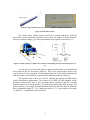

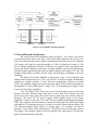
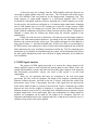
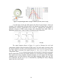
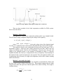

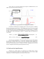
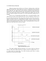


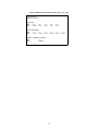


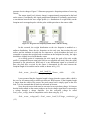
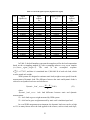
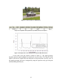
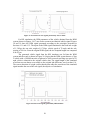
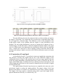

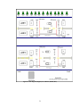

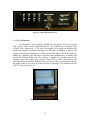
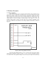

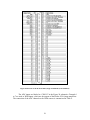

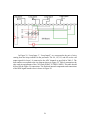


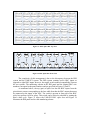
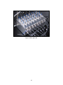


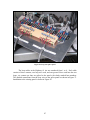
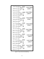
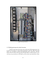
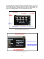


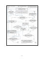
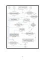
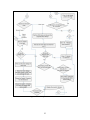


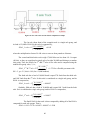


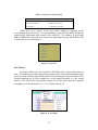

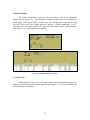


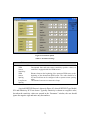
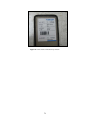
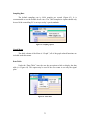
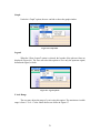
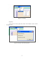

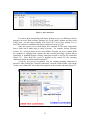


![2013 Gun List internet copy[2]](http://vs1.manualzilla.com/store/data/005851443_1-16b4e1bd3fc391c408d2005c48a2e336-150x150.png)