Download Auto-connection technique in primitive part modelling

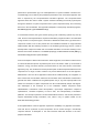
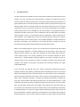
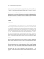
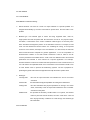
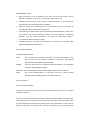
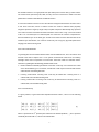
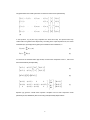
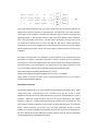
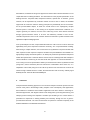
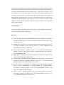
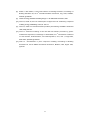
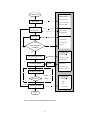
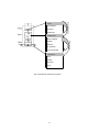
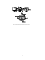
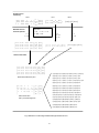
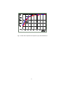
Auto-connection technique in primitive part modelling
T.T. Chow*, C.L. Song
Division of Building Science & Technology, City University of Hong Kong, Tat Chee Avenue,
Hong Kong, China,
*Corresponding author, fax: 852-27889716; email address: [email protected]
Abstract
In thermal simulation, an approach to satisfy the diversifying simulation objectives is to provide
a simulation environment that is capable to process the represented thermal system
dynamically and to the desirable level of detail. In the component- based modeling approach
adopted in contemporary building simulation software, the components in the plant library
often cannot truly reflect the actual system performance. For some years, efforts have been
placed on the search for alternative simulation environment. Primitive part (PP) modeling has
been one of these efforts. It possesses most of the attributes of a desirable environment such
as flexible, input-output independent, hierarchical modeling structure, detailed and unified
fundamental approach. This paper describes the background of PP modeling, and the
auto-connection data flow structure that facilitates the model developer to synthesis simulation
components from PP sub-models through user interface.
Keywords: Numerical simulation, thermal models, primitive part modeling, data structure
1. Introduction
Mathematical representations of thermal processes in building fabric and environmental control
systems are highly non-linear and involving time -dependent parameters. Nevertheless, heat
transfer fundamentals are essentially the same applying to the building envelope and the plant
system. In thermal simulation, what requires to satisfy the diversifying simulation objectives is a
simulation environment that is capable to process the represented thermal system dynamically
and to the required level of detail. The way to achieve this is by establishing sets of
conservation equations for different spatial regions, and then arranging for solving these
equations over the time span. In a numerical s ense, this is to couple building and plant in the
thermal model by gathering the energy and flow balance equations, often in the matrix form, for
both the building side and the plant side. The equation set is then solved either directly or by
iteration [1].
If we look back to the earlier stages of developments of building simulation in 70’s and 80’s,
the simulation software by that time provided detailed analysis of the thermal processes
through building fabric, but incorporated only with a simplified steady state plant energy
1
performance representation [2]. The oversimplification in system simulation resulted in the
overwhelmingly use of arbitrary and predefined parameters. This menu-based approach was
later on replaced by the component-based simulation approach. The component -based
approach allows the users to build a system network resembling the actual physical plant
through the selection of system components from a plant component library, and connecting
them as if in the real situation. This approach is adopted in contemporary simulation programs,
like TRNSYS [3], ESP-r [4] and ENERGYPLUS [5].
In real situation however, the types and the topology of air-conditioning system vary case by
case. Their accurate representation requires the simulation program be able to accommodate
a large number of component types, and levels of abstraction within each type. Most of the
component models in use at the present time are inflexible and based on range-restricted
empirical data. With the continuing evolution in air-conditioning te chnology, there is a need to
develop better component models and more flexible simulation environment. Working in this
direction were various endeavors – the SPARK project [6], the Neutral Model Format (NMF) [7],
and the IDA code [8] are some quoted examples.
From the viewpoint of thermal and fluid flow in HVAC equipment, it has been found that some
27 sub-model elements (known as primitive parts or PP’s as listed in Table 1) can be used to
model the energy and mass transfer processes based on the finite volume conservation
approach [9,10]. The combination of these primitive parts could well represent different HVAC
components at a range of levels of detail. The process -based nature of the PP approach
differentiates it from the other approaches named above. Mathematically, the integration of
PP’s at each node of a simulation network is the summation of the individual PP coefficients to
generate the matrix coefficients of the global equation set [11,12]. This super-imposition rule
makes the construction of plant components from PP’s mathematically simple and elegant.
The advantages of the technique lie in the contribution towards component model
standardization, hierarchical model decomposition, input-output independent component
representati on, controlled complexity of source code, and inter-operability of simulation
platforms. The technique provides a unified mathematical structure, and has the potential to
support extensibility through inheritance, and, offers a way to update models as the
state-of-the-art technology evolves.
A full implementation of the PP approach requires the availability of a graphical environment,
such that the PP synthesis of plant components can be worked through a user-friendly
computer interface. A description of the auto-connection data flow structure is the main
purpose of this article.
2
2.
PP Auto-connection
The flow chart in Figure 1 illustrates the PP modeling and simulation process through the user
interface. The user, most often the model developer, is expected to possess the technical
know-how about the nature and functions of each PP and the associated physical laws. For a
given simulation task, the user should review and define well the purpose and the scope of the
specific problem at hand. He should develop the overall thermal model and sort out the plant
components in need. In the process, the user is to con vert his physical plant into a simulation
model making reference to the available PP’s from the PP library. The equipment should be
categorized according to the HVAC common classification, like fans and pumps, flow conduits,
heat exchangers, and so on. This facilitates systemic categorization of plant components for
future reference. The available types of PP as at present allow the execution of dynamic
thermal simulation on basic HVAC systems. In its expanded application, a modest extension of
PP library is envisaged. This means that a user should be able to develop his new PP
sub-models and inserts them into the PP library when the need arises in future.
With the PP modeling approach, the PP’s are connected at the interface level with material
type and fluid type identified. A connection between two PP sub-models is the merge of two
selected nodes to become one, which then represents the same spatial region within the
overall thermal system. The concept is different from the connection between two plant
components in component-based modeling approach. The latter is virtually the pass of
operation data from one component to another. The built-in connection rules allow program
checking of the validity of a connection, say whether the connection is between two ‘legal’
nodes at different PP’s.
At the next step, th e technical data o f the system components, including their physical
properties, features, and operating conditions should be available for user input. This technical
data is node-related rather than component-related. The control data for use in the simulation
pro cess should also be stated at this stage. The PP models so far developed are based on
finite volume conservation equations. The input and operating parameters are divided into
three types : state variables, static data and dynamic data . The state variables data (i.e. nodal
temperature and mass flow rates) is updated through the solution process at every iteration
step. The s tatic data (including the control data) is user defined and is read from either the
user interface or the simulation input file. The dynamic data (such as fluid density and viscosity)
is computed based on the above two types of data as derived parameters. With these three
types of parameters, all matrix coefficients can be obtained in every iteration step through the
coefficient generator. Their numerical values are passed to a matrix equation solver through
3
which the solution at each time step is obtained.
The last step of the simulation procedure is result analysis. Both graphical analysis and
tabulated result files should be available. User judgment and validation test can be exercised
to observe the quality of the th ermal model. Sensitivity tests can be used to check the
importance of certain energy flow path by either the addition or the deletion of some PP’s in
the model. In our auto -connected PP system structure, the node parameters, control data, and
matrix coefficients can be grouped and exported as an input data file. To facilitate data transfer,
transformation program is to be developed to convert such data file to a format recognized by
other popular simulation software (one example is the ‘.dck’ file for use in TRNSYS).
3. Data flow
3.1. Data structure
A key factor of developing a plant component, as well as the entire HVAC system, by
auto-connecting the PP’s lies in how the parameter array can be formed, with the data handled
in the correct order. Our discussions on the data structure will be based on a practical example
of synthesizing an insulated water pipe model, as illustrated in Fig. 2. This insulated water pipe
model is constructed by three PP’s: PP2.4 ‘surface convection with ambient; 1 node (deno ted
by S) ’ ; PP1.1 ‘ thermal conduction for solid to solid; 2 nodes (denoted by M and N)’; and PP4.3
‘flow upon surface for 1-phase fluid; 3 nodes (denoted by S, WM and W1)’. Mathematical
derivation of the conservation equation sets of this model has been reported elsewhere [13]
and will not be repeated. Instead, the data format in the auto-connected system will be
introduced.
Three levels of basic data can be found in an auto-connected PP system: the node level, the
PP level, and the component level. A nod e is a region of physical space where the thermal
state is described by the conservation equation set. So nodes are ‘space oriented’. One level
up is the PP’s that are ‘process oriented’. 27 of them are currently in the PP library. Then the
third level is the component level. The plant components are ‘function oriented’ and can be
arranged to form an HVAC system model. Besides these three levels of data, there are
information on the links between different nodes and different PP’s. These links are referred as
the connection data, each of which is characterized as either ‘node’ connection or ‘PP’
connection. All kinds of data involved have distinctive attributes that differentiate them from the
others.
4
3.2. Data Attributes
3.2.1. Node Attributes
Node attribute s include the following:
²
Name/ Identifier: The name of a node is a unique identifier in a specific problem. It is
assigned automatically by the auto-connected PP system when the user starts a new
problem.
²
Material type: Four material types or nature are being supported: solid, moist air,
single-phase fluid and two-phase fluid. No restrictions are set for the physical shape,
orientation, or dimensions of the nodes of different material types, not until they have
been selected and assigned a position in the simulation network. For example, a solid
node can well describe the interior surface of a ventilating fan casing, or the exposed
surface to a duct heater, all subject to the user definition . For fluid nodes, the technical
data involved should b e a dequate for general applications, i.e. for the computation of
dimensionless numbers or the heat transfer coefficients. Listed in Table 2 are the
common parameters associated with the nodes o f the four different kinds . Not all listed
parameters are essential or even relevant for a specific application. For example,
effective diameter is relevant for a solid node that represents an inner conduit surface, but
not a flat surface. Encapsulated mass of air is insensitive to the simulation results in lots
of moist airflow cases in practical air-conditioning systems. The list is prepared for
preserving the generic nature of the PP approach and to help the users in specific cases.
²
Node type:
Incoming node:
this acts as input information and indicates the end of the former
connection.
Contact node:
this associates with physical quantities for solving in the matrix solver.
Leaving node:
this also associates with physical quantities for solving in the matrix
solver; functionally it acts as output and indicates the sta rt of another
connection in the system.
Ambient node:
this provides the boundary condition data. In our system, the ambi ent
node is a part of the PP sub -models, as in PP1.2 and PP2.4. Thus the
time-varying boundary conditions are read through the ambient-type
PP sub-models.
3.2.2. PP Attributes
5
PP data attributes include:
²
Name: The name of a PP is referenced to the name of such PP sub -model in the PP
database. For instance, 011 is for PP 1.1, 043 for PP4.3, and 101 for PP 10.1.
²
Identifier: This is the unique name of a PP in a specific problem. It is automatically set
each time when a PP is selected from the PP database.
²
Nodes list: Nodes are the building blocks of PP sub-models. Thus the node list is an
information table about the elements in a specific PP.
²
PP parameter: An address table named PP parameter address database is built to store
the numerical data. These parameters include the thermal properties , the physical
attributes , and
the derived parameters.
The latter are determined through a
communication interface with the user inputs.
²
Connection identifier : This stores the link address of a specific PP in a problem, which
helps the program itself to locate such PP.
3.2.3. Component Attributes
Component attributes include:
Code:
The component code is based on the HVAC component classification. It acts
like the ‘type’ and ‘unit’ defined in TRNSYS or HVACSIM+. This attribute
expands component utilization and its compatibility.
Identifier:
This is the unique name of a component in a specifi c problem . It is automatically
set when a specific problem is defined.
Description: This is a text description used to outline a specific problem for future reference.
PP list:
PP’s are the building blocks of a component. PP list is an array providing
information on these building elements of a specific component.
3.3. PP connections
3.3.1. PP connection attributes
There are two kinds of connection in the auto -connected PP system: the PP inner connection
and the PP connection.
A PP inner connection describes the thermal and flow interaction between the nodes within
one primitive part. It is a program level connection. Heat and mass transfer among the nodes
is the physical behavior represented by the PP model. This is described as a part of the PP
attribute in PP models. To exemplify this connection, consider PP4.3 in Fig. 3 that describes
6
the thermal behavior of a single-phase fluid (like water) when it flows along a solid surface.
The 3 fluid nodes (denoted by W0, WM, and W1 ) are inner connected to model a fluid flow
phenomenon. This link is described as one feature of PP4.3.
A connection between two PP’s occurs when the user assigns a link between two PP’s. This is
a user level connection, which in essence means two nodes in different PP’s physically
merged to represent a region (a single node) of a plant component. Numerically they represent
one node in the solver and share the same information of this node. In Fig. 3 , the solid node M
of PP1.1 is connected (and so combined) with the solid node S of PP2.4 to represent the
thermal insulation layer of the water pipe. M and S thus share the same technical data of the
insulation layer. Sometimes, one of the two nodes may not occupy any physical space before
merging, such as the incoming node.
3.3.2. Auto Connection Rules
To guard against incorrect links between nodes from two different PP’s, auto -connection rules
are built in the code to help the user. In our system, several kinds of link errors and warning
messages have been incorporated. Incorrect links have been made an automatic failure.
These are to guard against the following possible human errors:
²
Nodes of different material types linked: Connection could only occur between two nodes
of the same material type. For instance, a solid node could only be connect ed with another
solid node, but not a flowing fluid node.
²
Incoming nodes linked: Incoming node could only be linked with a leaving node or a
contact node, but not another incoming node.
²
Leaving nodes linked: a leaving node could only be linked with an incoming node or a
contact node, but not another leaving node.
3.3.3 .Connection theory
In a given problem, a typical PP matrix template with three nodes I, J and L is in the following
format:
 A( k, i, i )
 A(k , j , i )

 A( k, l , i )
A(k , i, j )
A(k , j , j )
A( k, l, j )
where k represents the k
th
A( k, i, l )  I 
A(k , j , l ) × J  =
A(k , l , l )  L 
 B (k , i ) 
 B (k , j ) 


B (k , l ) 
(1)
primitive part selected in the defined problem; i , j and l represent
numerically the node order of I, J and L in the overall matrix.
7
The global matrix of an overall system with ‘S’ number of nodes can be represented by:
C( 1,1 ) C ( 1,2 ) .. C ( 1 ,m ) .. C( 1, s )  I   D( 1 ) 
C( 2 ,1 )
:
C( 2 , s )  II   D( 2 )

 :
:
:     : 

×  = 

..
.. C ( n ,m ) .. C( n , s )  :   D( n )
C( n ,1 )
 :
:
:     : 

   

..
.. C( s ,m ) .. C( s ,s )  S   D( s )
C( s ,1 )
(2)
In the equation, C(n,m) and D(n) represent the future time step and present time step
coefficients in the global matrix respectively. According to the super-imposition rule, the matrix
coefficients C(n,m) and D(n) can be given by the summation of PP coefficients, i.e.
s
C (n, m) = ∑ A(i , n, m)
(3)
i =1
s
D(n ) = ∑ B (i, n )
(4)
i =1
To construct the insulated water pipe model, the sub-matrix templates of PP1.1, PP2.4 and
PP4.3 in the PP library are respectively
 A(11,1) A(11,2) M   B(11,1)
 A(11,3) A(11,4) ×  N  =  B(11,2)

   

(5)
[A( 24,1 )] × [S ] = [B( 24,1 )]
(6)
 A( 43,1 )
 A( 43 ,4 )

 0
A( 43,2 )
A( 43,5 )
A( 43,8 )
 S 
 
  B( 43,1 )
WM

 =  B( 43,2 )
A( 43,6 ) A( 43,11 ) × 

W 1  
 
A( 43 ,9 )
0
  B( 43 ,3 )
W0 
0
0
(7)
Equation (8) gives the overall matrix equation template of this 4-node component model
(denoted by S1, S2, WM and W1) with one incoming node (denoted by W0) as follows:
8
 S1 
0
0
0  
 C( 1,1 ) C( 1,2 )
 D( 1 ) 
S 2  
C( 2 ,1 ) C ( 2 ,2 ) C( 2 ,3 )


0
0
D( 2 )

 × WM  = 

 0
C( 3 ,2 ) C ( 3 ,3 ) C( 3 ,4 ) C ( 3 ,5 ) 
  D( 3 )

 W1  

0
C( 4 ,3 ) C( 4 ,4 )
0  
D( 4 )
 0
W 0  
(8)
This overall matrix template for the pipe can be derived from the conventional approach by
setting the conservation equations. At the same time, the coefficients of this matrix equation
can be given by the summation of primitive part coefficients. Figure 4 shows an example of the
data flow process. In this example, the user made connections between nodes of different
PP’s in the order of PP4.3, then PP1.1, and then PP2.4. Accordingly, the node order (or the
row number of the matrix) from 1 to 5 is for S2, WM, W1, W0, and S1. This is purposefully
made different from those in equation (8) to demonstrate that the data structure can support
different assigned node order and can arrive at the same required values of the overall matrix
coefficients.
If a specific simulation task is to investigate the thermal behavior of the insulated water pipe
with respect to changes in inlet water temperature conditions, equation (8) or the equivalent
one built by PP’s becomes the global matrix of the defined problem. The program identifies the
coefficients index of auto-connected PP and dynamically set the matrix coefficients in the
course of simulation. Figure 5 gives the simulation results of two specific flow cases:
o
o
Case1: Step change in inlet water temperature from 5 C to 10 C.
o
o
Case2: Linear change in inlet water temperature from 5 C to 10 C in 10 seconds.
These results are exactly the same as the one developed directly from the conventional
component-based modeling approach.
4. Flexibility Vs Complexity
The benefit of applying PP’s is to allow a flexible and generalized representation of the HVAC
system under study. A pre-requisite for the convenient use of the PP’s is then to make
available in the input interface an adequate data set of commonly used parameters in system
simulation. These will include technical data such as physical dimensions (like length,
thickness, volume etc.), material properties (like density, specific heat, conductivity etc.) and
heat and mass transfer coefficients at various flow conditions (like piped flow, wind induced
airflow, natural convection, wet surfaces etc.). The input parameters should be readily
availabl e at a friendly and practical user interface. For those less commonly used parameters,
the user is allowed to insert the additional information based on their own technical knowledge
or experimental research of the situation under study.
9
Nevertheless, a limitation of this generic approach is that the data in HVAC simulation is more
complicated than in building simulation. The data structure of the physical specification of the
building structure: composite walls, transparent surfaces, opened door or windows, ground
surfaces, can be represented by a handful number of rules or laws. In HVAC, the available
equipments are enormous and thei r working principles vary dramatically from one to another.
As the process-related objects, to obtain the overall model of the topologically complex
thermal system is non-trivial. In the missing of an important heat transfer coefficient of a
complex geometry for instance, the user has to either dig out the most relevant formulae
through rigorous literature search, or do their own laboratory research to find out the
correlation expression. This is so far one basic barrier encountered in system simulation when
opted for the explicit modeling approach.
From a practical point of view, a step towards the wider use of PP’s can be to narrow down the
applicability of the plant components whenever necessary, as in component-based modeling.
When facing a complex situ ation, user could mix the PP-synthesized component models with
other empirical or semi -empirical component models in the plant database. Also feasible is to
appropriately simplify the thermal system in an attempt to produce PP-synthesized component
models that operate with a reduced data set. At this end, PP modeling lends itself to adapt to
various situations in treasuring for the state-o f-the -arts approach to numerical simulation . A
4-row cooling coil can be represented in detail by an extensive 20-node PP-synthesized model
(using PP4.3, PP4.4 and PP5.2) that can examine the condensation rate at each row, or a
simplified 3 -node model (using PP4.3 and PP10.3) with the heat removal from the moist air
stream through a wetted surface in contact; the heat extraction rate can be any arbitrary figure
stated by the user. These are where the flexibility lies.
5.
Conclusions
Component-based modeling approach in the numerical analysis of thermal system has been
used for some years in the building industry. Despite of the contemporary wide applications,
their limitations of restrictive and monolithic applications has led to efforts in searching for
alternative approaches, with targets at better code management, promoting data sharing, and
satisfying ever-increasing user aspirations. Primitive part modeling is one of these efforts. It
possesses its uniqueness in offering flexibility and uniformity through the use of generic
process-based elements. The auto-connected PP ca n provide a controlled complexity of the
software architecture of an advanced numerical tool.
10
A key factor in the data structure that makes possible the auto -connection of PP’s has been a
systematic array of parameters and matrix coefficients that can be called upon efficiently and
accurately. The data attributes at each of the three levels – node, PP, and component – have
been elaborated in the article. Also explained are the connection attributes together with the
connection theory and rules. An insulated water pipe has been quoted as an example to
demonstrate the details behind the rules and the techniques that allow the overall matrix
coefficients be built dynamically. A pre-requisite for the use of the PP’s is then to make
available in the input interface an adequate data set of general parameters that are popularly
used in system simulation.
Acknowledgement
The authors express our thanks to the financial support of the Strategic Research Grant
7001114 from the City University of Hong Kong.
References
[1]
Clarke JA. Prospects for truly integrated building performance simulation, Proceedings of
th
Building Simulation ’99, the 6 International IBPSA Conference, Sep 1999, Kyoto, Japan,
Vol.3, pp.1147-1154.
[2]
Stoecker WF. Procedures for simulating the performance of components and systems
for energy calculations, 3rd ed. American Society of Heating, Refrigerating, and
Air-Conditioning Engineers Inc., Atlanta, 1975.
[3]
Solar Energy Laboratory. TRNSYS Version 15, user manual and documentation,
Madison, Wisconsin: Solar Energy Laboratory, Mechanical Engineering Department,
University of Wisconsin, 2000.
[4]
ESRU. ESP-r: a building and plant energy simulation environment: user guide version 9
series, University of Strathclyde, Glasgow, 2000.
[5]
Crawley DB et al., ENERGYPLUS: New capabilities in a whole-building energy simulation
th
program, Proceedings of Building Simulation 2001, the 7
International IBPSA
Conference, Aug 2001, Rio de Janeiro, Brazil, Vol.1, pp.51-58.
[6]
Buhl W F, Erdem FC, Winkelmann FC, Sowell EF. Recent improvements in SPARK:
strong component decomposition, multivalued objects, and graphical interface,
th
Proceedings of Building Simulation ‘93, the 3 International IBPSA Conference, Aug
16-18, 1993, Adelaide, Australia, pp.283-289.
[7]
Sahlin P, Bring A, Kolsaker K. Future trends of the Neutral Model Format (NMF),
th
Proceedings of Building Simulation ‘95, the 4 International IBPSA Conference, Aug
14-16, 1995, Madison, Wisconsin, USA, pp.537-544.
11
[8]
Sahlin P. IDA modeler, a man -model interface for building simulation, Proceedings of
Building Simulation ‘93, the 3
th
International IBPSA Conference, Aug, 1993, Adelaide,
Australia, pp.299-305.
[9]
Clarke JA. Energy Simulation in building design, 2
nd
ed. Butterworth-Heinemann, 2001.
[10] Chow TT, Clarke JA, Dunn A. Primitive parts: an approach to air -conditioning component
modeling, Energy and Buildings, 1997; 26: 165-173.
[11] Chow TT, Clarke JA. Theoretical basis of primitive part modeling. ASHRAE Transactions
1998; 104(2): 299-312.
[12] Chow TT. Numerical modeling of fluid flow and heat transfer processes by generic
fundamental components, Proceedings of HEFAT2002, the 1
st
International Conference
on Heat Transfer, Fluid Mechanics, and Thermodynamics, Vol.1, Part 1, Kruger Park,
South Africa, April 2002, pp.302-307.
[13] Chow TT.
Generalization in plant component modelling. Proceedings of Building
Simulation '95, the 4th IBPSA International Conference, Madison, USA, August 1995,
pp.48-55.
12
Simulation Task
Function Description
Problem Description
Component Category
Define Problem
Component Description
Environment Details
…
Select PP’s
10 PP Categories
from PP Library
27 Primitive Parts
Connect PP’s
Connection Rules
Connection Index
Check
PP Links
Connection Validity &
NO
Completeness
YES
Data Description
Input Parameters
Input system operation data
Control Data & Rules
Input Data Editing
Translator
Complete Input Data File
Transformation:
Input Files for other
Simulation Platforms
Coefficient Generator
Solution
Matrix Solver
Process
Result Analysis
Result Files
Figures
NO
Charts
Satisfactory Outputs?
Contour Maps
YES
End
Fig.1. Flow chart of PP modeling and simulation process
13
Name/Identifier
Node type
Material type
Node Connection
Node
Node
Primitive Part
Name in database
Nodes list
PP parameters
Connection identifier
Component
Code
Identifier
Description
PP list
Fig. 2. Data structure of PP auto-connection
14
PP Connection
Identifier
Fig. 3. Insulated water pipe model formed from PP models
15
PP Sub-matrices
in PP library
PP4.3
 A(43,1)
 A(43,4 )

 0
A(43,2 )
A( 43,5 )
0
A( 43,6 )
A (43,8 )
A( 43,9 )
Global PP-matrices
In defined problem
k=1
S → S2
 A( 1 ,1,1 )
 A( 1,2 ,1 )

 A( 1,3,1 )

 A( 1,4 ,1 )
A( 1 ,1,2 )
A( 1,2 ,2 )
A( 1,3 ,2 )
A( 1,1,3 )
A( 1,2 ,3 )
A( 1,3 ,3 )
A( 1,4 ,2 )
A( 1,4 ,3 )
PP1.1
 S 
0
 
  B (43,1) 
W M 

A(43,11) × 
= B (43,2 )
  W1  

 
0
  B( 43,3) 
W 0 
 A (11,1)

 A(11,3)
PP2.4
A (11, 2)  M   B (11,1) 
×   = 

A (11, 4)  N   B (11,2) 
[ A(24,1)] × [S ] = [B(24,1)]
Node order:
1 – S2 3 – W1
2 – WM 4 – W0
A( 1 ,1,4 )  S 2 
A( 1,2 ,4 ) W M
 ×
=
A( 1,3 ,4 )  W 1 
 

A( 1,4 ,4 )  W 0 
 B ( 1,1 )
 B( 1,2 )


 B( 1 ,3 )


 B( 1,4 )
5 – S1
k=2
M → S2
N → S1
 A ( 2 ,5 ,5 )
 A( 2 ,1 ,5 )

A( 2 ,5 ,1 )   S 1   B ( 2 ,1 ) 
×
=
A( 2 ,1 ,1 )   S 2   B ( 2 ,2 ) 
k=3
S → S1
[ A( 3 ,5,5 )] × [S 1] = [B( 3 ,1 )]
Global overall matrix
 C( 1,1 )
 C( 2 ,1 )

 C( 3 ,1 )

 C( 4 ,1 )
 C( 5 ,1 )
C( 1,2 ) C( 1,3 ) C( 1,4 ) C (1 ,5 )  S 2 
C( 2,2 ) C( 2 ,3 ) C( 2 ,4 ) C( 2 ,5 ) W M
 

C( 3,2 ) C( 3 ,3 ) C( 3 ,4 ) C( 3 ,5 ) ×  W 1  =
 

C( 4 ,2 ) C( 4 ,3 ) C( 4 ,4 ) C( 4 ,5 )  W 0 
C( 5 ,2 ) C( 5 ,3 ) C( 5 ,4 ) C( 5 ,5 )  S 1 
 D( 1 ) 
D ( 2 )


 D( 3 )


D ( 4 )
D ( 5 )
C(1)=C(5,5)=A(1,5,5)+A(2,5,5)+A(3,5,5)=0+A(11,1)+A(24,1)
C(2)=C(5,1)=A(1,5,1)+A(2,5,1)+A(3,5,1)=0+A(11,2)+0
Global overall matrix built by PP’s
C(3)=C(1,5)=A(1,1,5)+A(2,1,5)+A(3,1,5)=0+A(11,3)+0
C(4)=C(1,1)=A(1,1,1)+A(2,1,1)+A(3,1,1)=A(43,1)+A(11,4)+0
C(5)=C(1,2)=A(1,1,2)+A(2,1,2)+A(3,1,2)=A(43,2)+0+0
0
0
0   S1 
 C( 1 ) C( 2 )
 C( 3 ) C( 4 ) C( 5 )
0
0 )   S2 

 

 0
C( 6 ) C( 7 ) C( 8 ) C( 11 ) × W M  =

 

0
C( 9 ) C( 10 )
0  W 1 
 0

  W 0 
C(6)=C(2,1)=A(1,2,1)+A(2,2,1)+A(3,2,1)=A(43,4)+0+0
C( 12 )
C( 13 )


C( 14 )


C( 15 )
 0 
C(7)=C(2,2)=A(1,2,2)+A(2,2,2)+A(3,2,2)=A(43,5)+0+0
C(8)=C(2,3)=A(1,2,3)+A(2,2,3)+A(3,2,3)=A(43,6)+0+0
C(9)=C(3,2)=A(1,3,2)+A(2,3,2)+A(3,3,2)= A(43,8)+0+0
C(10)=C(3,3)=A(1,3,3)+A(2,3,3)+A(3,3,3)= A(43,9)+0+0
Global overall matrix
built by conventional approach
C(11)=C(2,4)=A(1,2,4)+A(2,2,4)+A(3,2,4)= A(43,11)+0
C(12)=D(5)=B(1.5)+B(2,5)+B(3,5)=0+B(11,1)+B(24,1)
C(13)=D(1)=B(1,1)+B(2,1)+B(3,1)=B(43,1)+ B(11,2)+0
C(14)=D(2)=B(1,2)+B(2,2)+B(3,2)=B(43,2)+0+0
C(15)=D(3)=B(1,3)+B(2,3)+B(3,3)=B(43,3)+0+0
Fig.4. Data flow in constructing insulated water pipe model from PP’s
16
Fig. 5 . Outlet water temperature in response to pi pe inlet disturbances
17
Table 1 List of primitive parts
1
Thermal conduction
1.1
solid to solid
1.2
with ambient solid
2
Surface convection
2.1
with moist air
2.2
with 2-phase fluid
2.3
with 1-phase fluid
2.4
with ambient
3
Surface radiation
3.1
with local surface
3.2
with ambient surface
4
Flow upon surface
4.1
for moist air; 3 nodes
4.2
for 2-phase fluid; 3 nodes
4.3
for 1-phase fluid; 3 nodes
4.4
for moist air; 2 nodes
4.4
for 1-phase fluid; 2 nodes
5
Flow divider and inducer
5.1
Flow diverger (for all fluid)
5.2
Flow multiplier (for all fluid)
5.3
Flow inducer (for all fluid)
6
Flow converger
6.1
for moist air
6.2
for 2-phase fluid
6.3
for 1-phase fluid
6.4
for leak-in moist air from outside
7
Flow upon water spray
7.1
for moist air
8
Fluid injection
8.1
water/steam to moist air
9
Fluid accumulator
9.1
for moist air
9.2
for liquid
10
Heat injection
10.1 to solid
10.2 to vapor-generating fluid
10.3 to moist air
18
Table 2 Parameters associated with different material types
Material Type
Solid
Basic Parameters
Type of material
Length, m
Total mass, kg
Width, m
2
Contact surface area, m
Effective diameter, m
2
Thermal resistance, m .K/W
View factor
Heat injection rate, W
Moist air
Mass flow rate, kg/s
Working pressure, Pa
Encapsulated mass, kg
Heat injection rate, W
Moisture content, kg/kg dry air
Dynamic viscosity, kg/m.s
3
Density, kg/m
Thermal conductivity, W/m.K
Specific heat, J/kg.K
Prandtl number
2
Single-phase fluid
Contact surface area, m
Entering air temperature, °C
Type of fluid
Working pressure, Pa
Mass flow rate, kg/s
Heat injection rate, W
Encapsulated mass, kg
Dynamic viscosity, kg/m.s
3
Density, kg/m
Thermal conductivity, W/m.K
Specific heat, J/kg.K
Prandtl number
2
Two-phase fluid
Contact surface area, m
Entering fluid temperature, °C
Type of fluid
Working pressure, Pa
Mass flow rate, kg/s
Dryness fraction
Encapsulated mass, kg
Heat injection rate, W
3
Density, kg/m
Dynamic viscosity, kg/m.s
Latent heat of evaporation, J/kg
Thermal conductivity, W/m.K
Specific heats, J/kg.K
Prandtl number
2
Contact surface area, m
Entering f luid temperature, °C
19