Download DISTRIBUTED DISPATCHING FOR EMBEDDED GENERATION

DISTRIBUTED DISPATCHING FOR EMBEDDED GENERATION
Stephen J. Conner, BEng
A thesis submitted for the degree of Doctor of Philosophy
Energy Systems Research Unit
Department of Mechanical Engineering
University of Strathclyde
Glasgow, United Kingdom
August 2003
© 2003 Stephen J. Conner
The copyright of this thesis belongs to the author
under the terms of the United Kingdom
Copyright Act as qualified by University of
Strathclyde
Regulation
3.51.
Due
acknowledgement must always be made of the
use of any material contained in, or derived from,
this thesis.
ii
“Imagination is more important than knowledge.”
-Albert Einstein
iii
ACKNOWLEDGMENTS
First of all I would like to thank my supervisor, Professor Joe Clarke, for advice,
guidance, and proofreading and corrections of the piles of paper I dumped on him.
I am also grateful to the Carnegie Trust for the Universities of Scotland, who funded
this project.
Thanks are also due to my fellow students, researchers and academics in ESRU, who
were always full of helpful advice and interesting ideas. In particular, Nick Kelly and
Iain Macdonald, who gave me a lot of assistance in the computer simulation side of
matters, and Paul Strachan who introduced me to LabVIEW, an amazing piece of
software which I used almost everywhere.
This project involved a lot of lab work, and a lot of custom-built equipment. I am
very grateful to all of the technical staff who made things for me, lent me apparatus,
and generally did things that were beyond the call of duty: Pat McGinness, Eric
Duncan and the Energy Systems technicians, Donnie and Dino from DMEM, Bill
Rooney and Bob Baird from the Department of Electrical Engineering, Alex Cairney
from Dynamics and Control, and Jim Docherty.
I was also fortunate in that, when funds began to run out, I found a part-time job with
an employer who understood the difficulties of juggling work and study, and made
sure that I was able to carry on with my research. That job turned out to be very
interesting and challenging in its own right. So thank you Ivan Andonovic, and
everyone else at Kamelian Ltd., for keeping my cash flow healthy and giving me my
first U.S. Patent.
Last but not least, I owe a debt of gratitude to my family, who gave me great moral
support throughout this whole business, not to mention putting a roof over my head
for some of the time.
iv
Dedicated to the memory of my grandfather
Ian Kitchener Colburn (1916-1972)
Physicist and lover of knowledge
v
ABSTRACT
Electrical power systems are currently moving towards distributed generation, using
many small generators instead of a few large ones. This can potentially produce great
improvements in efficiency, by allowing utilisation of waste heat (cogeneration).
However, it also poses new problems of control and co-ordination of large numbers
of generators, which may be connected deep within the distribution network. It is
well known that existing schemes for planning, dispatching and protection of central
generators are not directly applicable to the new technolo gy, and dispatching
(scheduling) of small embedded generators is not currently feasible.
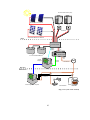
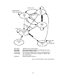
In this work, a novel dispatching management system which may meet this
requirement is proposed. Instead of using a single control centre, it distributes
dispatching functions throughout the network. Some functions are performed by
controllers and software agents built into the embedded generators themselves, and
others handled by dispatcher software associated with a group of generators and
loads. The dispatcher operates a small virtual market where energy can be traded
between agents representing: generators, loads, network functions (AVR etc), and
other dispatchers. This allows multiple dispatchers to be interconnected, so
potentially dealing with very large numbers of generators.
To test this concept, some prototype agents, a basic dispatcher, and means of
communication were created, in the form of programs on a desktop computer. The
“REDMan” suite of software achieved successful trading of energy in a simulated
environment. This motivated a more advanced trial where REDMan was developed
further and used for experimental dispatching of real generating equipment and
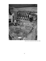
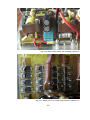
loads. Construction and assembly of the experimental apparatus, interfacing of
hardware to the computer environment, experiments and results are presented and
discussed here. The experimental system was dispatched in a satisfactory manner,
and much practical experience was gained in the issues relating to dispatching of EG.
Several possible avenues for further research were identified.
vi
CONTENTS
CHAPTER 1:PREFACE.....................................................................................................................................I
CHAPTER 2:BACKGROUND........................................................................................................................3
2.1. THE USE AND WASTE OF ENERGY .......................................................................................................... 3
2.2. GENERATION AND TRANSMISSION OF ELECTRICITY........................................................................... 6
2.3. THE NEW IDEA : EMBEDDED GENERATION............................................................................................ 8
2.4. THE TECHNOLOGY OF EG ...................................................................................................................... 9
2.5. CONNECTING EG TO THE GRID............................................................................................................ 11
2.6. A LOOK AT DISPATCHING..................................................................................................................... 12
2.6.1. Predicting demand..........................................................................................................................12
2.6.2. Coping with the unexpected..........................................................................................................13
2.6.3. Economics........................................................................................................................................13
2.6.4. Renewables......................................................................................................................................13
2.7. THE FUTURE OF DISPATCHING............................................................................................................. 14
2.7.1. Alternatives to classic dispatching..............................................................................................15
2.8. CONCLUSIONS........................................................................................................................................ 16
2.9. REFERENCES .......................................................................................................................................... 16
CHAPTER 3:POWER SYSTEMS CONTROL ........................................................................................18
3.1. HOW DOES CONTROL APPLY TO POWER SYSTEMS? .......................................................................... 18
3.2. LOAD FREQUENCY CONTROL............................................................................................................... 19
3.2.1. Simple governor..............................................................................................................................19
3.2.2. Implementation in large networks...............................................................................................20
3.3. A UTOMATIC VOLTAGE REGULATION .................................................................................................. 20
3.3.1. Fundamentals..................................................................................................................................21
3.3.2. How AVR is set up ..........................................................................................................................22
3.3.3. AVR considerations for EG...........................................................................................................22
3.4. PROTECTION........................................................................................................................................... 23
3.4.1. Types of protection equipment......................................................................................................23
3.4.2. Protection for EG ...........................................................................................................................24
3.4.3. Anti-islanding protection...............................................................................................................24
3.5. IMPACT OF EG ON EXISTING CONTROL SYSTEMS ............................................................................. 26
3.6. ECONOMIC DISPATCHING..................................................................................................................... 26
3.6.1. Theory...............................................................................................................................................26
3.6.2. Application to EG ...........................................................................................................................28
3.7. STABILITY.............................................................................................................................................. 28
3.7.1. What exactly is stability?...............................................................................................................28
vii
3.7.2. Classical stability studies..............................................................................................................29
3.7.3. Application to EG systems ............................................................................................................30
3.7.4. How will EG affect stability?........................................................................................................31
3.7.5. EG might improve stability...........................................................................................................31
3.7.6. Or perhaps not................................................................................................................................32
3.8. CONCLUSIONS........................................................................................................................................ 33
3.9. REFERENCES .......................................................................................................................................... 34
CHAPTER 4:A NEW DISPATCHING SYSTEM PROPOSED ...........................................................37
4.1. DISTRIBUTED DISPATCHING................................................................................................................. 37
4.1.1. Embedding LFC and AVR.............................................................................................................37
4.1.2. Embedding ED ................................................................................................................................38
4.1.3. Embedding demand prediction.....................................................................................................38
4.2. ECONOMIC CONSIDERATIONS.............................................................................................................. 38
4.3. THREE SIMPLE RULES FOR DISPATCHING........................................................................................... 40
4.3.1. The rules...........................................................................................................................................40
4.3.2. Assumptions underlying the rules................................................................................................41
4.4. REDM AN PROPOSED ............................................................................................................................ 43
4.4.1. Algorithm and communications...................................................................................................43
4.4.2. Timestepping considerations........................................................................................................48
4.4.3. Timestepping and commitment.....................................................................................................48
4.4.4. Handling concurrency...................................................................................................................49
4.5. PROVING THE CONCEPT ........................................................................................................................ 49
4.6. DESIGNING AN EXPERIMENT................................................................................................................ 51
4.7. CONCLUSIONS........................................................................................................................................ 51
CHAPTER 5:DEVELOPING THE REDMAN SOFTWARE...............................................................52
5.1. THE DISPATCHER................................................................................................................................... 52
5.2. DETAILS OF PROGRAMMING ................................................................................................................ 55
5.3. W RITING THE PROGRAM....................................................................................................................... 55
5.4. TESTING.................................................................................................................................................. 56
5.4.1. Worked example..............................................................................................................................57
5.4.2. Speed test..........................................................................................................................................60
5.4.3. Speed test results.............................................................................................................................62
5.5. VALIDATION........................................................................................................................................... 62
5.6. COMMUNICATIONS................................................................................................................................ 63
5.6.1. Ethernet networking.......................................................................................................................63
5.6.2. DSTP/DataSocket ...........................................................................................................................64
5.6.3. Testing DSTP/DataSocket.............................................................................................................65
viii
5.6.4. Results...............................................................................................................................................66
5.7. REDM AN COMMS ROUTINES............................................................................................................... 67
5.7.1. Data items to be transferred .........................................................................................................67
5.7.2. Allocating index numbers..............................................................................................................68
5.7.3. Timing and synchronisation..........................................................................................................69
5.7.4. Realisation of the system...............................................................................................................69
5.7.5. Latency, quality of service, etc .....................................................................................................70
5.7.6. Some sample agents .......................................................................................................................71
5.8. OUTCOMES AND CONCLUSIONS........................................................................................................... 71
5.9. REFERENCES .......................................................................................................................................... 72
CHAPTER 6:BUILDING A TESTBED ......................................................................................................73
6.1. GRID-CONNECTED WORKING............................................................................................................... 74
6.2. GENERATING PLANT ............................................................................................................................. 75
6.2.1. Dispatching PV/wind energy ........................................................................................................75
6.2.2. Using batteries................................................................................................................................76
6.2.3. Inverters ...........................................................................................................................................77
6.3. CONSIDERATIONS IN SETTING UP T HE SYSTEM ................................................................................. 77
6.3.1. Choosing voltages and power levels...........................................................................................79
6.3.2. Measuring power flow...................................................................................................................80
6.4. SETUP AND COMMISSIONING ............................................................................................................... 81
6.4.1. Equipment list..................................................................................................................................81
6.4.2. Structure...........................................................................................................................................82
6.4.3. Layout...............................................................................................................................................84
6.4.4. Power wiring...................................................................................................................................84
6.4.5. Signal wiring...................................................................................................................................89
6.4.6. Testing ..............................................................................................................................................90
6.5. SUMMARY .............................................................................................................................................. 90
6.6. REFERENCES .......................................................................................................................................... 91
CHAPTER 7:AGENT SOFTWARE ............................................................................................................92
7.1. A BATTERY MANAGEMENT AGENT ..................................................................................................... 92
7.1.1. Why batteries?.................................................................................................................................92
7.1.2. How lead-acid batteries work.......................................................................................................93
7.1.3. Variation of capacity with discharge rate..................................................................................93
7.1.4. Factors affecting battery voltage.................................................................................................95
7.1.5. Ageing and service life...................................................................................................................95
7.1.6. Calculating energy content: not easy?........................................................................................96
7.1.7. A simpler battery management model.........................................................................................96
ix
7.1.8. Estimating capacity........................................................................................................................97
7.1.9. Taking care of batteries.................................................................................................................98
7.1.10. Using these ideas..........................................................................................................................99
7.1.11. A model for battery wear and tear.......................................................................................... 100
7.1.12. Practical implementation......................................................................................................... 102
7.1.13. Practical implementation......................................................................................................... 104
7.1.14. REDMan connection................................................................................................................. 108
7.1.15. Testing BatMan.......................................................................................................................... 108
7.2. INVERTER AGENT.................................................................................................................................110
7.2.1. Design............................................................................................................................................ 110
7.2.2. Prototype....................................................................................................................................... 110
7.2.3. Calculating inverter efficiency.................................................................................................. 111
7.2.4. Simple fixed-price algorithms.................................................................................................... 111
7.2.5. Economic dispatch Mark One ................................................................................................... 112
7.2.6. Economic dispatch Mark Two................................................................................................... 112
7.3. GENERATOR AGENT ............................................................................................................................114
7.4. DUMP LOAD AGENT .............................................................................................................................114
7.4.1. Implementation............................................................................................................................. 115
7.4.2. Performance ................................................................................................................................. 115
7.5. DEMAND AGENT ..................................................................................................................................117
7.5.1. The original.................................................................................................................................. 117
7.5.2. Smart Socket ................................................................................................................................. 118
7.5.3. Prototype power-measuring agent............................................................................................ 118
7.6. SUMMARY ............................................................................................................................................122
7.7. REFERENCES ........................................................................................................................................122
CHAPTER 8:EXPERIMENTS ................................................................................................................... 125
8.1. SUMMARY OF DEVELOPMENT WORK SO FAR...................................................................................125
8.1.1. Software......................................................................................................................................... 125
8.1.2. First hardware ............................................................................................................................. 126
8.1.3. Mark Two hardware.................................................................................................................... 126
8.1.4. Mark Two software...................................................................................................................... 126
8.2. EXPERIMENT DESIGN ..........................................................................................................................127
8.3. TESTING DISPATCHER.........................................................................................................................128
8.4. CHECK AGENT PROGRAMS/ASSUMPTIONS .......................................................................................129
8.5. TESTING COST MODELS ......................................................................................................................129
8.5.1. Inverter cost model...................................................................................................................... 130
8.5.2. Battery cost model....................................................................................................................... 130
8.5.3. Interactions................................................................................................................................... 130
x
8.6. EXAMINING MULTIPLE DOMAINS ......................................................................................................130
8.7. OBJECTIVES OF EXPERIMENTS...........................................................................................................131
8.8. SUMMARY ............................................................................................................................................131
CHAPTER 9:RESULTS OF EXPERIMENTS ...................................................................................... 133
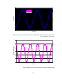
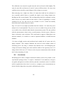
9.1. TEST RUN FOR ENERGY BALANCE/TRANSIENT ................................................................................133
9.2. ENERGY BALANCES.............................................................................................................................135
9.3. DAQ HARDWARE CHECK...................................................................................................................136
9.4. INVERTER RE -TEST ..............................................................................................................................138
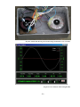
9.5. TRANSIENT BEHAVIOUR .....................................................................................................................140
9.5.1. Typical dispatching behaviour.................................................................................................. 140
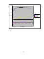
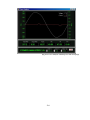
9.5.2. Actual/dispatched power flows comparison............................................................................ 142
9.5.3. In search of missing energy ....................................................................................................... 142
9.6. TWO-DOMAIN INTERACTION..............................................................................................................145
9.7. SUMMARY ............................................................................................................................................145
9.8. REFERENCES ........................................................................................................................................146
CHAPTER 10:.........................................................................................................................CONCLUSIONS
147
10.1.
DOES IT DISPATCH SUCCESSFULLY?............................................................................................147
10.2.
DOES IT WORK ECONOMICALLY?.................................................................................................147
10.3.
W ILL IT SCALE TO LARGE NUMBERS? .........................................................................................148
10.4.
OVERALL CONCLUSIONS...............................................................................................................148
10.5.
FURTHER WORK..............................................................................................................................149
10.5.1. Hardware.................................................................................................................................... 149
10.5.2. Software issues........................................................................................................................... 149
10.5.3. Marginal cost............................................................................................................................. 149
10.5.4. Multi-domain issues.................................................................................................................. 150
10.5.5. Concurrency and commitment handling................................................................................ 151
10.5.6. Penalties...................................................................................................................................... 151
10.5.7. Combined heat and power dispatching................................................................................. 152
10.5.8. New Electricity Trading Arrangements................................................................................. 152
10.5.9. Politics/economics/subsidies................................................................................................... 152
10.5.10. Strategic barriers to implementation................................................................................... 153
10.6.
A FINAL WORD................................................................................................................................154
APPENDIX A: BUILDING AN INVERTER ........................................................................................ 155
A.1.
W HAT IS AN INVERTER?................................................................................................................155
A.2.
W HY BUILD AN INVERTER?..........................................................................................................155
A.3.
DESIGN OBJECTIVES ......................................................................................................................156
xi
A.4.
SPECIFICATION ...............................................................................................................................157
A.5.
BASIC DESIGN CHOICES.................................................................................................................157
A.5.1. Switching technologies............................................................................................................... 158
A.5.2. Circuit topologies........................................................................................................................ 158
A.5.3. Control algorithms...................................................................................................................... 161
A.6.
SIMULATION ...................................................................................................................................163
A.7.
PRACTICAL DESIGN ISSUES ...........................................................................................................163
A.8.
CONTROL CIRCUITS........................................................................................................................168
A.8.1. PWM generator........................................................................................................................... 168
A.8.2. Switching logic............................................................................................................................. 168
A.8.3. Drive circuits ............................................................................................................................... 172
A.8.4. Reference generator.................................................................................................................... 174
A.8.5. Choosing a processor................................................................................................................. 175
A.8.6. Firmware ...................................................................................................................................... 176
A.8.7. Support circuitry.......................................................................................................................... 176
A.9.
BUILDING AND TESTING THE M ARK ONE...................................................................................177
A.10.
LESSONS LEARNT FROM M ARK ONE...........................................................................................180
A.10.1. Odd spikes.................................................................................................................................. 180
A.10.2. Excessive losses......................................................................................................................... 180
A.10.3. Too much distortion.................................................................................................................. 180
A.10.4. Latch-up...................................................................................................................................... 181
A.11.
M ARK TWO.....................................................................................................................................181
A.11.1. Loss budget ................................................................................................................................ 181
A.11.2. Transistors.................................................................................................................................. 182
A.11.3. Current sense resistor.............................................................................................................. 182
A.11.4. Wiring ......................................................................................................................................... 182
A.11.5. Transformer ............................................................................................................................... 182
A.11.6. Filter components..................................................................................................................... 184
A.12.
A SSEMBLY AND SNAGGING ..........................................................................................................185
A.13.
TESTING THE M ARK 2 ...................................................................................................................190
A.14.
LESSONS LEARNT FROM THE MARK 2.........................................................................................193
A.15.
PROTECTION ...................................................................................................................................194
A.16.
NOTES ON FIRMWARE....................................................................................................................195
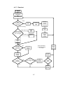
A.17.
FLOWCHART ...................................................................................................................................197
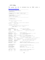
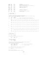
A.18.
LISTING............................................................................................................................................198
A.19.
REFERENCES...................................................................................................................................204
APPENDIX B: A VOLTAGE-CONTROLLED DUMP LOAD ...................................................... 206
B.1.
DESIGN CONSIDERATIONS.............................................................................................................206
xii
B.2.
CIRCUIT ...........................................................................................................................................207
B.3.
COMPUTER INTERFACE ..................................................................................................................208
B.4.
CONSTRUCTION..............................................................................................................................208
APPENDIX C: THE “SMART SOCKET”............................................................................................ 211
C.1.
DESIGN CONSIDERATIONS.............................................................................................................211
C.2.
INTERFACING..................................................................................................................................213
C.3.
CIRCUIT DESCRIPTION...................................................................................................................213
APPENDIX D: POWER MEASUREMENT BY SOUNDCARD .................................................... 217
D.1.
DESIGN CONSIDERATIONS.............................................................................................................218
D.2.
HARDWARE.....................................................................................................................................218
D.2.1. Current transformer ................................................................................................................... 218
D.2.2. Voltage transformer ................................................................................................................... 219
D.2.3. Circuit........................................................................................................................................... 219
D.3.
SOFTWARE ......................................................................................................................................219
D.3.1. Data gathering ............................................................................................................................ 219
D.3.2. Analysis ........................................................................................................................................ 220
D.4.
CALIBRATION AND TESTING.........................................................................................................220
D.5.
CONCLUSIONS.................................................................................................................................221
APPENDIX E: MODELLING INVERTERS IN ESP-R ................................................................... 225
E.1.
A BOUT STRUCTURE OF ESP-R ......................................................................................................225
E.2.
THE POWER FLOW SIMULATOR (PFS) .........................................................................................226
E.3.
A CTIVE CONNECTIONS ..................................................................................................................226
E.4.
A DDING NEW POWER COMP ONENTS............................................................................................228
E.5.
RESULTS..........................................................................................................................................228
E.6.
CONCLUSIONS.................................................................................................................................230
E.7.
A CKNOWLEDGEMENTS........................................................ERROR! BOOKMARK NOT DEFINED .
E.8.
REFERENCES...................................................................................................................................230
APPENDIX F: HYBRID PV SYSTEM CONTROLLER ................................................................. 231
F.1. A BOUT THE SYSTEM............................................................................................................................231
F.2. CONTROLLER REQUIREMENTS...........................................................................................................231
F.3. DESIGN CONSIDERATIONS..................................................................................................................231
F.4. THEORY OF OPERATION ......................................................................................................................232
F.5. CIRCUIT DESCRIPTIONS.......................................................................................................................232
F.5.1. Controller module....................................................................................................................... 232
F.5.2. Power supply/metering module................................................................................................ 233
F.5.3. System wiring............................................................................................................................... 233
xiii
F.6. M ODIFICATIONS ..................................................................................................................................234
APPENDIX G: HOW LABVIEW WORKS .......................................................................................... 240
G.1.
W HAT IS LAB VIEW? ....................................................................................................................240
G.2.
W HAT IS IT USED FOR?..................................................................................................................240
G.3.
BASICS OF LAB VIEW PROGRAMMING .......................................................................................241
G.4.
DATA TYPES....................................................................................................................................243
G.5.
CONDITIONAL EXECUTION............................................................................................................243
G.6.
M ATH FUNCTIONS..........................................................................................................................243
G.7.
M ULTITASKING ..............................................................................................................................244
G.8.
M ODULARITY .................................................................................................................................244
G.9.
DOCUMENTING LAB VIEW PROGRAMS ......................................................................................244
G.10.
REFERENCES...................................................................................................................................245
APPENDIX H: LABVIEW PROGRAMS .............................................................................................. 246
H.1.
THE TESTBED SOFTWARE ..............................................................................................................246
H.2.
BLOCK DIAGRAMS (SOURCE ) OF SELECTED VIS ........................................................................248
H.2.1. BatMan battery management (bm2.vi).................................................................................... 248
H.2.2. BatMan state-of-charge estimator (bmestimator.vi)............................................................ 253
H.2.3. Smart inverter management (invman7.vi) .............................................................................. 255
H.2.4. REDMan dispatching server (server3.vi)............................................................................... 261
H.2.5. REDMan dispatching algorithm (matching15.vi)................................................................. 266
xiv
Preface
This Ph.D. started out with only a very general brief: To reduce the harmful effects
of fossil fuel combustion. At the outset, this was easily mistaken for a technological
problem, and it was tempting to believe that there was some kind of magic bullet to
be discovered which would make engines and boilers more efficient, or which would
make renewable energy sources so cheap, reliable, and tempting that it would not
even be worth bothering with oil.
The first task undertaken was a literature review, trawling books, journals, and the
Internet for background information. This gave cause for suspicion that the problem
was of a different nature. There were many examples of new technologies, great
improvements over the status quo in terms of combustion efficiency or harvesting of
renewable energies, like biodiesel, the Coates engine, cogeneration, affordable
electric drives for cars, and even the old-fashioned bicycle. The magic bullets were
all ready and waiting. Why was nobody pulling the trigger?
Of course, energy use is not a technological problem at all, but a complex sociopolitical one. Reactionariness and fear of change are embedded into every society
and institution, denial is a part of everyday life, and people will probably never drive
electric cars because they don’t make a revving noise. Large amounts of money are
invested in maintenance of the status quo, short-term profit is pursued irrespective of
long-term consequences, and there is nothing that engineering can do about any of
this.
However, there did seem to be one or two small areas that might be susceptible to
technological advances. Distributed generation was a recent, fairly radical concept in
which large central electric power stations are replaced by large numbers of small
generators. If these are sited carefully where heat is also demanded, perhaps in each
domestic dwelling or public building, the waste heat inherent in electricity generation
need not go to waste. With further study, it became apparent that this concept was
missing one important component: a way of controlling all the small generators,
synchronising them together so that they worked in harmony, keeping all the
advantages of the old electrical grid. No record could be found in the public domain
1
of any work towards this objective, and so it seemed like a promising avenue for
research.
The first step was to study the automatic generation control systems used in ordinary
power networks. The tendency in these was for generation to be scheduled centrally,
and it was obvious that this would never work with distributed generation, where a
network might contain millions of units. If it was to be successful, the control system
would have to be distributed too.
There are not many precedents for control systems of this kind. A rough analogy can
be drawn with biological systems, e.g. plants and rudimentary animal life- forms.
These all showed the same tradeoff: by forfeiting a centralised control, they became
more robust, but sacrificed intelligence and functionality. According to this analogy,
it seemed probable that some elements of traditional power networks would need to
be sacrificed. But, it seemed hopeful that nothing much would be lost in the sacrifice,
that much of the intelligence thrown away from the top might be reborn from the
bottom up as an emergent property of the large, complex system made from the
interconnection of many small ones.
With this in mind, an effort was made to abstract the automatic generation
control/dispatching process to the simplest set of rules possible without actually
making it useless. These rules were implemented in computer software, as modules
which could be distributed over networked machines. The results were encouraging,
and motivated the construction of a small renewable energy generating plant on
which to test the new control system.
This pilot plant was a success, demonstrating desirable behaviour which would be
impossible with existing EG control systems. However, there are still very many
questions to be answered, and issues to be explored, before the “REDMan” system
could see real-world applications. The work documented in this thesis is really just
one drop, and it can only be hoped that future years, and the changing climates and
priorities of the world, will bring on the ocean that distributed generation needs.
Stephen Conner
Glasgow, November 2002
2
Chapter 2: Background
This chapter presents the findings of the initial literature review, by way of
background. It looks at how energy is used, citing statistics on global energy
production and consumption, with a view to finding out where energy is wasted, and
whether this waste is avoidable. Out of various possibilities, cogeneration of heat and
electricity is selected as a promising way of reducing energy waste, and investigated
further. Problems which prevent the wider use of cogeneration are identified and
explored in greater detail.
2.1. The use and waste of energy
As a rough estimate, the Earth’s human population currently use 11.6 terawatts
(tera=1012 ) of all kinds of power in the course of their daily business [1]. Of this,
approximately 3% comes from renewable sources, and 7% from nuclear power, but
the remaining 90% is from fossil fuels. Estimates of the size of fossil reserves
suggest that natural gas might run out in approximately 20 years, oil in 50-70 years,
and coal in perhaps 200 years. From then on, nuclear and renewable energy will be
the only options. As far as nuclear energy is concerned, the risks associated with
radioactive waste, and nuclear plant accidents, are well known. The cost of providing
safety measures against these risks, combined with adverse public opinion, has
seriously hindered the nuclear industry. For example, [3] states that no new reactors
have been ordered in the United States since 1979.
So, fossil fuels are running out, and nuclear energy is unlikely to step up to take their
place. Therefore, future energy scenarios are likely to involve reducing demand, and
increasing the amount of energy drawn from renewable sources. Reduction of
demand will be considered first. An excellent way of doing this is reducing waste of
energy, so it is logical to ask the question: Where do the greatest wastes of energy
take place? Detailed studies [e.g. 1, 2] have been made of energy use patterns, and
some representative figures* are presented here.
*
These figures are average power flows over a one-year period.
3
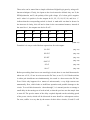
Of the 11.6TW consumed as primary fuels:
5 TW (43%) is used in electricity generation, which is approximately 35% efficient,
so 1.75 TW of electricity is the result.[1]
4.2 TW (36%) is used for heating of buildings, domestic hot water, and industrial
processes [2]
1.9TW (16%) goes to transportation of people and goods. [2] The vast majority of
this is of fossil origin. Motor vehicle engines convert about 20% of the fuel energy
into mechanical work.
Of course, the question of what proportion of this energy is actually wasted is a
difficult one. In transportation, for example, not all journeys are necessary. In
heating, the insulation of buildings can always be made better. And, there are many
uses of electricity which might not be considered indispensable. Finding answers to
these questions would require a detour into politics, economics, and the social
sciences. But, from an engineering perspective, it is obvious that a lot of energy is
being wasted in electricity generation and transport. Unfortunately, this is for a
fundamental reason.
All engines which convert heat to mechanical work, whether they be petrol engines
in cars, or steam turbines in electric power stations, have a theoretical maximum
efficiency imposed by the Second Law of thermodynamics. The theory behind this is
well known, and will not be repeated in detail here. Suffice it to say that in a vapourcycle heat engine the theoretical limit is the Carnot efficiency:
? ? 1?
tl
th
(Eq 2.1)
In modern thermal power stations, the materials used will stand source temperatures
of around 800 K, and by rejecting heat straight to ambient, a sink temperature of
around 300 K is possible. This equates to a Carnot efficiency of 63%. Of course, as
any text on thermodynamics will tell, the Carnot efficiency can only be attained if all
heat transfers in the cycle are reversible, which means that they must take place
across zero temperature difference, and therefore be infinitely slow, and hence
4
useless. In practice, irreversibility caused by heat transfer across finite temperature
differences, mechanical friction, etc. reduces the conversion efficiency to 35-40%.
For example, [5] quotes a mean efficiency of 37% for power stations in the UK.
With regard to transport, internal-combustion engines are somewhat different; their
theoretical benchmark is the air-cycle efficiency, which is a function of the
compression ratio r.
? ?1
?1 ?
? ? 1? ? ?
?r?
(Eq. 2.2)
State-of-the-art engines currently have compression ratios of between 8 and 16,
which give air-cycle efficiencies of 56% and 67% (assuming ?=1.4 for air)
respectively. Again, though, in real life the best IC engines are about 40% efficient
[4] when operated at their optimum speed and load. In transport applications, the
widely- varying speed and load reduce the overall efficiency even further.
The point of quoting all these statistics is to suggest that, as regards improving the
efficiency of heat engines, it may be a case of diminishing returns. If, by some feat of
materials science, the absolute source temperature in a contemporary generating
plant could be doubled without melting anything, the Carnot efficiency would only
increase by 29%, which would probably mean at most a 16% increase in the actual
efficiency. That 16% would probably be bought at an enormous cost in terms of
elaborate materials, advanced design, and reduced reliability.
Another possibility might be to keep temperatures constant, but make up the shortfall
between the Second Law efficiency and real- life efficiency, by reducing
irreversibility. There are a number of innovative technologies, such as combinedcycle gas turbine plant, and bottoming cycles for steam plant, which are used to
boost efficiency in this way. The fundamental principle is to use several real cycles
in order to approximate the ideal cycle more closely. Unfortunately, the law of
diminishing returns holds true here too. Adding one bottoming cycle might half the
shortfall in efficiency, but to achieve the full Second Law efficiency would require
an infinite number of cycles. Therefore, the degree of improvement is again limited
by economic and technical considerations.
5
The one unchallenged assumption in all of this is that the heat rejected from a heat
engine is wasted. This is easy to overlook, because in contemporary power-plant
design, the heat is rejected at the very lowest temperature possible for efficiency’s
sake, and this makes it of no practical use. Deliberately raising the rejection
temperature a little opens up a number of new applications for this “waste” heat, for
example space heating, domestic hot water, and industrial process steam. This may
seem like anathema because it makes the conversion to work less efficient, but really
it does not matter any more; considering the rejected heat as a useful output, the
actual efficiency of the system becomes 85-90% [4]. The old ‘efficiency’ now just
determines the heat-to-power ratio. This concept is known as cogeneration, or
combined heat and power (CHP). It promises to yield much greater gains in
efficiency than any of the improvements to conventional heat engines discussed
previously.
Cogeneration schemes like these could obviously save a great deal of energy if they
were widely used, but this is unfortunately not the case: at the moment in Britain a
mere 6 % [5] of UK electricity comes from CHP plants. The reason for this neglect is
that there is a serious problem with large-scale use of CHP. The problem is
intimately connected with the way in which electricity is generated and used.
2.2.1 Generation and transmission of electricity
Currently, electricity is generated in large power plants situated some distance from
the point of demand. This system of ‘centralised generation’ dates from the late 19th
century. All electrical equipment of that era used direct current of low voltage, which
could not be transmitted more than a few miles without incurring excessive losses in
the conductors, or using very thick and costly conductors. The solution was to build a
small coal- fired generating plant on every city block, which was inconvenient,
inefficient, and expensive. Soon, better ways of transmitting power were invented* ,
to help in the exploitation of hydro-electric resources. This economical long-distance
power transmission brought in a massive expansion of electricity supplies, and
*
The three-phase high-voltage AC transmission system was first used in 1891 and still exists in
essentially the same form today.
6
allowed generating stations to be made as large as technically possible in order to
gain economies of scale. This trend of increasing size and centralisation has persisted
until the present day.
At present, in a country such as Britain, hundreds of generating stations, mostly sized
between 100MW and 1GW, feed three-phase AC power into a ‘national grid’ of
high- voltage (275-400kV) transmission lines which interconnect generators,
switching stations, and demand centres. The grid system provides redundancy, so
that if lines or generators fail, power can be quickly re-routed from elsewhere. The
sheer scale of this system is impressive; for example, the UK’s national grid handles
approximately 327TWh of energy per year, through more than 7,000 km of
transmission lines [6].
This may seem very impressive, but just because something is successful does not
mean that it is perfect, and it is now acknowledged that centralised generation has
one major drawback: It makes CHP almost impossible. This is because electricity
can be transmitted easily over hundreds of miles; but there is no comparable system
for transmitting low- grade heat from the place where it is generated to the points of
demand.
This is not its only failing, though; centralised generation can also have an effect on
reliability. If generation is concentrated in a few large units, then the failure of one of
these units will have a greater impact on the network. To protect against this,
network planners use ‘spinning reserve’. A power plant (or plants) of total capacity
equal to the largest single plant in use is kept idling and ready to pick up the load
immediately. This protects against the failure of any single generating plant, but at a
cost; even though this spinning reserve does not produce any power, it still uses fuel
to make up its thermal and mechanical losses.
Centralised generation also means increased losses; although the transmission system
is very efficient, it is not perfect. For example, [6] claims 1.7% losses for the UK
National Grid transmission system.
However, due to the enormous amounts of
electricity being transmitted, this represents a large loss in absolute terms, in this case
approximately 635 MW. This figure varies according to network configuration, and
7
does not include distribution losses, which are more difficult to measure, but are
probably of a similar magnitude or even larger.
2.3.1 The new idea: embedded generation
Fortunately, there is a new way of organising the electrical network. Instead of
having a few large generating stations, electricity generation can be subdivided into
smaller units spread throughout the network. This is known as distributed generation.
In the specific case where an effort is made to site generators as close as possible to
centres of demand, in such a way that buildings might almost be thought of as
generating their own power, it is termed embedded generation (EG).
This approach promises to solve many of the problems discussed previously. Firstly,
it makes CHP practical. Individual generators can be sited right at centres of heat
demand, so there is no problem with transmission. CHP benefits from smaller scale,
since the heat rejection temperature of each individual generator can then be tuned to
suit the process requirements: e.g. 50 OC for hot water, 150 OC for industrial steam.
And, if these small generators are connected with the existing electrical network,
there could be a reliability benefit due to the redundancy of multiple power sources.
This is a contentious point of view, though, which will be examined at greater length
in a later section.
Distributed generation can also help exploitation of renewable energy (RE).
Important forms of RE, such as wind and solar power, are diffuse by nature. They
can only be captured in large quantities by using a large number of distributed small
generators, covering a large area. It may be possible to embed large numbers of RE
generators in/on existing buildings and structures.
Finally, electrical transmission losses are greatly reduced, since the electricity is not
transmitted over any appreciable distance. For non-renewable sources, though, this
advantage is perhaps not as great as it seems, since some other fuel must be
transmitted instead. Transporting the fuel to the generator location uses energy too,
and this can be thought of as a transmission loss.
8
2.4.1 The technology of EG
Really, EG is just a return to Edison’s ‘powerhouse on every block’ system which
was abandoned 100 years ago. It may well become attractive again because of
improvements in small generator technology, and the efficiency improvements
promised by cogeneration. Small/medium heat engines suitable for cogeneration
have seen many advances: Pollution, reliability and noise control have been
improved, by borrowing technologies from automobile and aero-engine design.
Microprocessor control allows generators to operate automatically without
supervision. High-temperature ceramics and alloys together with computer-aided
design have increased the efficiency of smaller heat engines. Examples of these
modern heat engine technologies are: microturbines [7, 8] and IC engines [4]. These
are popular for cogeneration or backup power in the industrial and commercial
sectors. [9]
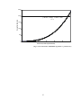
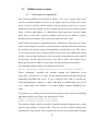
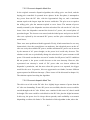
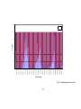
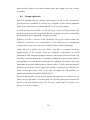
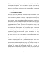
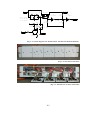
Renewable energy has seen improvements too. For instance, the cost of photovoltaic
modules has fallen steadily, as shown in fig. 2.1. Wind turbines have also become
more cost-effective, although it is harder to quantify prices in this case, because of
the variable nature of output [10]. Some renewable generators have also been
designed specifically for embedded generation, for example ducted wind turbines
which are an integral part of the building façade [11]. However, these are currently at
the experimental stage.
At present, renewable electricity is mostly uneconomic compared to fossil fuelgenerated electricity, hence such large PV and wind installations as there are mainly
exist because of government subsidies. However, wind power is rapidly becoming
competitive, and other forms of RE are expected to play an increasing part in the
long term, as fossil fuels become more expensive.
9
70
60
Module price (1994 const. US$/Wp)
Price ($/Wp), market (MWp)
.
World market (MWp)
50
40
30
20
10
0
1974
1976
1978
1980
1982
1984
1986
1988
1990
1992
1994
1996
Year
(Fig. 2.1: Price trend of PV, 1976-1994, reproduced from [12])
10
2.5.1 Connecting EG to the grid
The main problem lies in using EG alongside the existing electrical grid with its
centralised generators. While there is no fundamental reason why EG systems need
to be connected to the grid at all, there are advantages to doing so. Firstly, by
connecting multiple generators together to form a network, the reliability of the
supply might be improved due to redundancy. For the same reasons, it is also very
attractive to be able to combine the EG output with the existing grid. There are also
economic benefits: the efficiency of a generator is usually a function of its power
output, and so it is usually possible to calculate an optimum power for each generator
in a network in order to achieve the best overall efficiency. In a similar manner,
networking will make CHP more efficient, by making allowance for customers’ heat
demands as well. For example, if a customer with an embedded CHP plant has a
sudden large demand for he at, he can increase the output of his CHP plant, but then
he will find himself with surplus electricity. If his plant is connected to the grid, it
should be possible to sell this electricity to another customer.
But, it is also possible that as the network is made bigger, it will become more
complex, and the scope for error will increase too. As the system gets larger, the
dynamics get harder and harder to model. It would be almost impossible to predict
the transient performance, stability, response to faults, etc. of a network with
hundreds of thousands of embedded generators. Therefore, power companies and EG
manufacturers show a reluctance to move in this direction. There seems to be a great
lack of work on understanding the issues involved.
Managing an electrical grid is rather like commodity trading, but fraught with
difficulties because, unlike other everyday commodities, electrical energy is difficult
to store in any significant amount. Even when converted to another form of energy,
the possibilities for storage are limited, and some energy is always lost in the
conversion. Therefore, in practice, the supply must be continuously adjusted to
match the demand, and it must be done quickly, because the network does not have
much of an energy reserve. The only inherent energy storage is the rotating inertia of
the generators themselves, and any mismatch between supply and demand will
therefore alter the speed of the generators, and hence the frequency of the alternating
11
current. So, the first type of manageme nt required is load frequency control (LFC)
which adjusts the mechanical power driving the generators to hold the supply
frequency constant. Alongside this is economic dispatching (ED) which aims to
share out the total demand amongst the generators in such a way that they operate at
the best overall efficiency.
These jobs are collectively known as ‘dispatching’, and this will be the main
challenge that this hypothetical EG network will face: reconciling the traditional
methods of dispatching, developed on networks with a few large generating stations,
with the new requirements of EG. There seems to be no real idea of how to
accomplish this. As a source of inspiration, though, it may be instructive to examine
the way in which dispatching is currently done.
2.6.1 A look at dispatching
Dispatching was originally performed by a combination of simple automatic
controls, and people in a national control room, in contact with generating stations by
telephone. Human dispatchers have since been superseded by computerised
automatic generation control, but the objectives are still the same, and can be seen as
consisting of three fundamental parts; predicting demand, coping with unexpected
demand, and trying to reach an economic optimum.
2.6.1. Predicting demand
The demand for electricity in each half- hour period of the day is forecast one day in
advance. This is possible because there are daily and seasonal patterns in the
demand, related to working hours, mealtimes, television programming, and seasonal
heating/lighting requirements.
This system is satisfactory at present, but it should be borne in mind that the patterns
are predictable because they are the mean of the activities of a large number of
consumers. It is possible that, as the sample group is made smaller, as in a
hypothetical scenario where dispatching is distributed, its behaviour may become
more random, and prediction accordingly more difficult.
12
2.6.2. Coping with the unexpected
Prediction is never perfect, so there will always be some differences between
predicted and actual demand. Because of the size of a national grid system, these
tend to develop relatively slowly, and are not usually a problem. For example, if
demand begins to exceed supply, the angular momentum of the rotating machines
will make up the extra power. Therefo re, the generator speed, and hence frequency,
of the whole network will begin to decrease. As this happens, automatic control
systems will ramp up the mechanical power input to restore the frequency. Different
types of power plant vary in how quickly they can respond. So, operating within
these constraints, the dispatcher has to make sure that there is always enough plant
online, with enough spare capacity, and the capability to modulate its output quickly
enough, to deal with these unforeseen demand changes.
Of course, this assumes that the system is working properly. If there is a sudden,
violent disturbance, such as a fault, transient effects come in to play, and the effect
can be much more serious. Transient analysis of networks is a whole other subject,
though, and quite beyond the scope of this thesis.
2.6.3. Economics
Almost every type of generating plant is most efficient when operating at full power.
Part- load efficiencies are often very poor. Therefore, dispatching is also concerned
with maximising ‘utilisation’. Put simply, out of all the generators in operation, as
many as possible should be operated at maximum efficiency, which normally means
fully loaded. This is in conflict with the requirement for reserve capacity, and so a
trade-off has to be reached. The exact nature of this trade-off is a complicated issue,
because it sets the benefit due to quality of supply against the cost due to operating
the reserve capacity. In the UK, with its proud tradition of a nationalised electricity
industry where profit was less of an issue than quality of service, the value of a
dependable electricity supply is probably perceived to be quite high.
2.6.4. Renewables
When renewable energy is added to the supply pool, it causes new problems. The
main problem is that the most popular forms of renewable energy (hydro, solar and
13
wind power) are subject to the weather. Therefore, it is hard to predict exactly how
much will be available. This is really the same problem as coping with unexpected
demands, except in mirror- image. Wise design and siting of the renewable system
can help. At many sites in Scotland and Wales, for instance, wind and water are
relatively reliable and plentiful resources. Similarly, in areas like the south-western
US, sunshine is practically guaranteed most of the year. Also, the weather-related
behaviour of renewable sources often coincides with weather-related demand. For
example, in places like California, with sub-tropical climates, the output from solar
PV matches the demand from air-conditioning nicely. Similarly, in countries such as
Scotland, wind power increases in winter, in line with the increased heating and
lighting demand. What is more, modern weather forecasting is often reliable enough
that the output of wind/solar/hydro generating schemes can be predicted. However,
the vagaries of the weather mean that the problem can never be eliminated entirely,
and it is fairly certain that networks including large amounts of renewable generation
will need to cope with more extreme and unpredictable variations in supply, either by
using more reserve capacity, or by having some means of storing energy when there
is a surplus and releasing it when there is a shortfall [13]. Management of storage
systems like these would also fall under the remit of dispatching.
2.7. The future of dispatching
The main problem with current dispatching schemes, as described previously, is that
present algorithms are based on taking information about every generator in the
network back to a single control centre, calculating optimal setpoints for all the
generators, and then sending this information back. This is feasible in current
networks with 10-100 generating units, but in a future scenario with perhaps millions
of small embedded generators, it may well be impractical. For example, cons ider the
scenario where one in five UK households has replaced their domestic heating boiler
with a small grid-connected CHP unit. Instead of 100 generators, the control centre
has to deal with 5,000,000. Data flow to and from the control centre will increase by
four orders of magnitude, but the worst is yet to come. The amount of computing
power required to run the control algorithms is typically proportional to the square of
the problem size, if not some higher power. Therefore, the computing power required
14
will increase by at least eight orders of magnitude. To put this in perspective, by
Moore’s Law (which states that the power of computers doubles every 18 months) it
is around 40 years’ worth of development.
Of course, it might well be possible to mana ge such large amounts of data
successfully. But, objections can still be raised to the general concept of collecting all
data together to a central executive. The chief objection is that it represents a serious
reliability issue. If the control centre broke down, the whole network would be
rendered useless. So, it is a weak link in a system that should be strengthened by
redundancy. Also, because of its greatly increased complexity, the proposed control
centre might be more likely to break down than present-day systems.
Unfortunately, as may be seen in the following section, there do not seem to be any
more workable alternatives to this system at present.
2.7.1. Alternatives to classic dispatching
This section is based on a review of various EG systems currently available on the
market. The manufacturers’ published data, for example [7, 8], suggest that when
designing their systems they make one of two simplifying assumptions:
1. The generator is designed to be the sole source of power. It is governed so that it
supplies the correct amount of power to keep the terminal voltage and frequency
within limits. These ‘standalone’ generators are simply not designed for
connection to a grid; their output appears as a voltage source of low impedance,
making power flow into the network unstable and very difficult to regulate.
2. The generator is designed for network connection, but the decision of how much
power to generate at a given moment is left up to the end user, thus sidestepping
the dispatching problem completely. These ‘dumb’ generators will typically not
work unless they are connected to a large, stable electrical network.
NB: Some generators e.g. [8] can operate under either of the above modes, the
selection being made by the user.
A large-scale deployment of standalone generators would be inadvisable, to say the
least. An EG system made entirely of these, each feeding its own demand centre,
would throw away all the advantages of a grid. It would be very inflexible; if a
15
demand centre required more power than its generator could supply, the only
solution would be to buy a bigger one. Utilisation would be very poor too; the
generators would have to be sized to supply the peak demand, and in most cases the
mean demand is much less.
Connecting large amounts of dumb EG to the existing network would be equally
unwise, because it would lack any form of dispatching. There would be no guarantee
that supply would equal demand.
2.8. Conclusions
By reviewing the way in which electricity generation works at present, it was seen
that relatively large improvements in efficiency could be made by aggressive use of
CHP. But, to make CHP work, embedded generation is essential. There is reason to
believe that the full benefits of EG will not be realised unless it is networkconnected, and suitably dispatched to ensure stability and good economic use.
Unfortunately, it seems that the dispatching system presently used to control large
centralised power plants will not be practical for millions of small generators, nor
will the controls fitted to present-day EG solutions. Much work has been done on the
technical and economic implications of EG, and the need for a new kind of
dispatching system has been recognised [14], but there is no evidence of anyone
having investigated ways of making such a system. The objective of this project is to
do just that, but before producing any new ideas, a more detailed review of power
systems control is called for. This is presented in the next chapter.
2.9. References
1. ‘BP Global Statistical Review of World Energy’, 2001, http://www.bp.com/
2. ‘World Energy Prospects to 2020’, International Energy Agency, 2001,
http://www.iea.org/
3. ‘Nuclear Generating Units 1953-2001’, Energy Information Agency, USA, 2003.
http://www.eia.doe.gov/
4. ‘Cogeneration
with
Gas
Engines’,
http://www.jenbacher.com/
16
Jenbacher
Energy
AG.,
2003,
5. ‘Digest of United Kingdom Energy Statistics 2001’, Department of Trade and
Industry, http://www.dti.gov.uk/, p.168.
6. ‘Seven Year Statement’, National Grid plc., 2002, http://www.nationalgrid.com/
7. On-line
literature
from
Capstone
Turbine
Corporation,
2002,
http://www.capstone.com/
8. Bowman Power Systems, 2002, http://www.bowmanpower.com/
9. ‘U.S. Cogeneration: Beyond reduction of pollution’, Cogeneration and On-Site
Power Production, Vol. 1, No. 3. May-June 2000, pp. 25-33.
10. ‘Wind Energy – The Facts: Volume 2, Costs, prices and values’, European Wind
Energy Association, 1997, p. 56. Online at http://www.ewea.org/, 2003
11. ‘A hybrid PV/wind energy module for integration in buildings’, Proc. 16th
European Solar Photovoltaic Energy Conference, Glasgow, May 2000.
12. ‘Eco-restructuring: Implications for sustainable development’, ed. Ayres, R.U.,
United Nations University Press, 1998. Online at http://www.unu.edu/, 2003
13. “Wind on the System: Grid integration of wind power”, Renewable Energy
World, Vol. 3, No. 2, March/April 2000, pp. 61-71.
14. ‘Embedded Generation’, Jenkins, N. et al., IEE, London, 2000, p. 259.
17
Chapter 3: Power systems control
The need has been identified for a dispatching system that can control large numbers
of electrical generators without being excessively complicated. In order to have a
better idea of the requirements inherent in such a system, it will be wise to review the
control engineering aspects of power systems, to get a good impression of the issues
involved. This section is a brief review of power systems control; the techniques
used, the issues involved, and the technologies employed, with a particular bias
towards embedded generation. The reader is assumed to be familiar with some
fundamental concepts of control engineering itself, such as feedback and stability.
(See e.g. [1])
3.1.
How does control apply to power systems?
Control engineering is fundamentally concerned with applying a self-correcting or
self-regulating tendency to systems that do not naturally have such a tendency. This
concept is applied in many ways throughout the whole electrical power field.
However, in the sense of interest at present, power systems control essentially means
keeping voltage and frequency within acceptable limits for the consumer, while
operating the generating plant and transmission systems as efficiently and safely as
possible. This task can become very complicated in a large electrical network with
multiple generating stations, each with its own economic and dynamic behaviour,
connected together by a grid which has losses and constraints on possible power
flows. Multiple different control systems must work together without any negative
interactions arising. The functions performed by these control systems can be
grouped under a few very broad headings:
?
Frequency control, also known as load frequency control (LFC).
?
Automatic voltage regulation (AVR)
?
Protection
?
Economic dispatching (ED)
18
LFC is the system or systems that tries to keep the frequency of the supply constant.
It does this by increasing or decreasing the real power output from generators. AVR,
as the name suggests, tries to keep the voltage constant, or at least within limits for
all consumers. This may be done by tap-changing transformers which step the
voltage up or down slightly as required, or by devices which produce or consume
reactive power. Protection ensures that no component is overloaded to an unsafe
extent, by actuating circuit breakers in the event of a fault or overload. Lastly, ED
tries to ensure that all plant is operating as efficiently as possible.
These systems are often analysed in isolation, e.g. the protection system is studied
separately from all others. See [2] for examples. However, a little consideration of
the matter may give reason to believe that the various control systems interact. These
interactions are intentionally minimised in current power systems, but may become
more significant in EG systems. How this will happen is only beginning to be studied
(see e.g.[3]).
3.2.
Load frequency control
This is the most basic form of control in power systems. The idea behind it was
hinted at in the previous section, and can be restated in more detail here. Supply of
electricity must always equal demand. In an alternating current system, the frequency
of the AC is an indication of how good the supply/demand match really is. If demand
is greater than supply, the generators will begin to slow down and the frequency will
fall, etc. LFC senses any deviation from the nominal value of frequency, and changes
the mechanical power input to the generators, thus changing the real power injection
to the network, in order to restore the frequency to what it should be.
3.2.1. Simple governor
The simplest form of frequency control, where rotating generators are involved, is to
equip the engine/turbine (prime mover) with a governor that adjusts the fuel supply
to hold the rotating speed constant. This is the norm for many smaller types of
generator. However, in modern large National Grid-type networks, the scheme is
rather more complex.
19
3.2.2. Implementation in large networks
A large grid will have many different generating plants, of different kinds. Some are
capable of changing their power output quickly for LFC purposes, some are more
sluggish to respond, and some, for instance renewable energy plant, cannot be
controlled at all because they are determined by the amount of sun, wind, etc. present
at that time. This limitation can be dealt with as follows: All the generators are
connected together, therefore (within limits imposed by the configuration of the
network) it does not matter physically where the injection of real power needed for
frequency control comes from. In fact, the plant best suited to frequency control
duties might change on a daily or hourly basis. To make full use of this flexibility,
the modern trend is to schedule all generation on a minute-by- minute basis, via
commands sent from a grid control centre [4]. This is done by advanced computer
algorithms, which combine load- following control and economic dispatching. The
ED component calculates how the demand should be shared out amongst the
available generators, taking into account the reserves required for LFC. Large
networks are divided into areas, each containing one or more generators plus some
demand, and the ED algorithm also calculates how much power should be exchanged
between areas (tie- line power flow). The LFC algorithm combines frequency error
and tie- line power flow error in a given area to give a quantity known as the Area
Control Error (ACE). A controller algorithm is used to adjust the output of the
generator(s) in that area, in order to regulate the ACE to zero. Many different ways
of deriving the ACE, and many different control algorithms, such as ordinary P-I-D,
fuzzy logic, etc. are described in the literature. (e.g. [5, 6])
3.3.
Automatic voltage regulation
The frequency of alternating current is the same everywhere in the grid, but not so
voltage, which varies from place to place. Transformers step it up and down, and the
resistances and reactances of cables and lines cause the voltage to drop, or sometimes
even to rise, depending on the current passing. The purpose of AVR is to make sure
that every consumer gets a voltage within the statutory limits at all times.
20
3.3.1. Fundamentals
AVR systems are fundamentally the same as any other control system. The voltage at
a point in the network is measured, compared to a desired value, and the error signal
actuates some kind of voltage-adjusting device in such a way as to extinguish the
error. There are a few different types of voltage-adjusting device. One very widelyused type is the tap-changing transformer. This is like an ordinary distribution
transformer, but has a high-speed switch mechanism that changes the tapping point
on one or other of the windings according to the instructions of the AVR system [7,
8].
Another way of adjusting the voltage is by reactive power compensation [9]. This
works because transmission lines, transformers, etc. have an inductive component.
The inductive reactance of the system is usually much larger than the resistance and
so is responsible for most of the voltage drop. Therefore, connecting a capacitive
load can reduce the voltage drop, eliminate it completely, or even raise the voltage
above normal. Capacitors may be permanently installed, or switchable under control
of an AVR system. Another possibility is to use a synchronous motor, since these
have the ability to ge nerate or absorb reactive power as required. This may also
perform mechanical work, or it may be installed purely for power compensation, in
which case it is called a synchronous condenser. The synchronous generators used in
most large generating stations also have the same ability. Recently, power electronic
technology allowed the creation of the static compensator (STATCOM) which
performs the same function as the synchronous condenser, but without moving parts
[10]. Modern STATCOM/active filter systems are also capable of advanced
functions such as reducing harmonic distortion [11, 18].
Of course, reactive power compensation assumes that the network impedance is
mostly reactive. This may not always be the case, particularly in the distribution
network, which uses lower voltages (hence more resistive losses) and can have a
predominance of underground cables, which are not inductive but capacitive. Under
these conditions, reactive power compensation is less effective.
21
3.3.2. How AVR is set up
In an ideal world, the voltage would be regulated so closely that every consumer
received exactly the nominal voltage. This is not practical, so compromises have to
be made. The voltages in the HV transmission system are regulated by reactive
power compensation, performed by ge nerators and sometimes synchronous
condensers or capacitors. The aim here is as much to reduce losses by improving
power factor, as it is to keep the voltage constant. Large generating stations may
have an AVR system which controls the reactive power generation according to
network voltage [12] or alternatively the generation of reactive power may be
scheduled centrally. Indeed, a combination of the two is sometimes used, where
individual generators have their own AVR and LFC setpoints, which in turn are
controlled by central scheduling.
At the lower voltages used in the distribution system, tap-changing transformers are
preferred. There are so many of these that central control is not practical, therefore
they are normally controlled by their own local AVR, which is set so that the voltage
at the far end of the feeder never drops below the minimum acceptable. The AVR
may hold a constant voltage, or it may droop to allow current sharing between
paralleled transformers, or it may even have compounding which makes the voltage
rise as the current demand increases, to compensate for drop in the feeder. Finally, in
the furthest reaches of the distribution system, the transformers have no taps at all, or
taps selected by hand in a “set and forget” style.
3.3.3. AVR considerations for EG
Most embedded generation plant presently does not participate in AVR. This is for a
few reasons. Firstly, individual embedded generators are normally too small to have
any significant effect on network voltage. Of course there are some large EG units,
and it could also be argued that a lot of small generators could have the same
aggregate effect as a large unit. However, realising this would require some sort of
management system to make all the generators work together. This has been
proposed (see 3.5 below) but never tested. Secondly, some kinds of EG plant use
induction generators and so cannot perform reactive power compensation. This may
not be a great problem, since reactive power compensation is less effective deep in
22
the distribution network anyway [21]. On the other hand, there are other EG types
(such as PV, microturbines, and variable-speed wind turbines) that incorporate a
power electronic interface (inverter). This can simultaneously be used as a static
compensator for AVR purposes [22].
3.4.
Protection
Protection may be thought of as a control system too. It monitors the operation of
power system components such as lines, transformers and generators, and takes
action if the component is in a potentially dangerous state. That action is normally
the opening of a circuit breaker, which removes power completely from the
component. The goal of protection is to isolate faulty equipment as quickly as
possible, with minimal disruption to the supply of electricity, and minimal impact on
the stability (see 3.7 below) of the system.
3.4.1. Types of protection equipment
The most basic item of protection equipment is a fuse. Fuses provide simple and
reliable overcurrent protection, with a choice of response characteristics. However,
fuses are not suitable for many applications, because they require replacement by
hand before the power can be restored, amongst other reasons. Where this is a
problem, it is preferable to use a more complex system comprising protection relays
and circuit breakers. The protectio n relays are measurement devices which monitor
current, voltage, frequency, etc. When the measured value is outwith the set limits,
the protection relay sends a signal to the circuit breaker causing it to open. This
system offers greater flexibility: many different types of protection relays are
available e.g. earth leakage, phase imbalance, differential current, and several can be
wired together to operate one circuit breaker. Another very important feature is that
the breaker can be programmed to reclose by itself. Faults are often momentary in
nature, e.g. a lightning strike on overhead lines causing an arc to start. In cases like
these, opening the breaker clears the fault, and when it recloses, the system resumes
normal operation. If the fault did not clear, then the breaker will trip out again as
soon as it recloses, and after a few unsuccessful reclosing attempts, it will normally
trip out for good.
23
3.4.2. Protection for EG
Embedded generation has mostly the same protection systems as normal generating
plant, but with a few additional requirements. The first issue is that EG units of small
size, using synchronous or induction generators, cannot contribute much fault current
in the case of a fault on the distribution network. Sometimes the fault current is not
much more than the full- load current, or even possibly less. Nevertheless, it could
still hinder clearance of a fault, and so the distribution network must be protected
from it. Overcurrent protection on the EG unit itself cannot do this, though, because
the fault current flowing from the EG is too small. In this scenario, the fault will trip
protection elsewhere in the system, and isolate the section containing the fault and
EG unit. The EG will then hopefully trip out on over/undervoltage or other
protection [13]. If it did not trip, however, a power island might be the result.
3.4.3. Anti-islanding protection
If a part of the electrical network becomes separated from the rest due to a fault, and
it contains embedded generation, it might continue to function independently. Power
companies believe this to be unacceptable for three reasons; firstly, it would
endanger any personnel sent to repair the fault, secondly, the island would drift out
of phase with the rest of the network and it would be impossible to reconnect it
without causing a catastrophic transient, and thirdly, the power quality in the island
could not be guaranteed. On these grounds, they claim that the only safe way of
managing islanding is to forbid it; islands must be made deliberately unstable so that
they trip themselves out within a few seconds.
Unfortunately, these anti- islanding methods are exactly the opposite of what is
required for good network stability. For instance, if the frequency begins to collapse,
the grid needs a big injection of real power as quickly as possible. Instead, the rateof-change-of-frequency (ROCOF) protection systems commonly used with EG are
likely to trip out the embedded generators, which will take more real power away and
simply aggravate the collapse. A similar objection can be levelled at the SFS/SVS
anti- islanding algorithms for power electronic inverters [14]. Heavy penetration of
EG systems with this kind of anti- islanding protection would probably have
disastrous effects on network stability. So, it seems that if EG is to achieve
24
significant penetration, the current philosophy on islanding may have to change
completely.
The first objection, that islanding is unsafe, is perhaps not insurmountable. Electrical
engineers are all trained in safety, and always assume a circuit to be live unless they
have first- hand evidence to the contrary. It is probably more a matter of convenience
and expense than safety: embedded sources of power in the LV distribution system
would make fault location and repair much more difficult and time-consuming,
because there will no longer be a clearly-defined power flow from ‘generator’ to
‘load’. When the network stays live on both sides of a fault, how do you trace where
the fault is? Of course, the high- voltage transmission system faces this exact
challenge, and its solution is to use automatic protection relays that signal when and
where a fault has occurred.
There is a more serious side to this issue, however: if an embedded generator were to
trip out, and then restart at a later time while someone was working on the system, a
very dangerous situation could result. The protection systems currently used with EG
do not allow restarting unless a healthy voltage and frequency are already present,
and this is therefore one feature that should be kept.
The second objection is somewhat more grounded in fact, but again it need not be
insurmountable. If the power quality within an island was of a good standard, the
voltage and frequency would remain very close to that of the rest of the network.
Therefore, it might be possible to reconnect it at an instant when the relative phase
was correct. This phase-sensitive switching would require replacement or
modification of many breakers and reclosers in the existing system, and therefore
might not be economically desirable.
An alternative line of attack might be to ensure that islands never drift out of
synchronism at all. A very accurate timebase (to within a few nanoseconds) can be
derived from Global Positioning System (GPS) receivers. If enough generators in an
island were locked to the GPS timebase, and the generation in the rest of the network
was also locked, then there would be no problem. The price of GPS receivers is
currently around $150 and so this standard is accessible even to relatively small EG
units.
25
The final objection, poor power quality, is probably the most complex and
demanding of all. The network may island in a vast number of ways; in theory it can
split at any point where a fuse or circuit breaker is present. There is no way of
knowing whether generation will match demand within whatever islands might form.
The best approach here is probably to maintain tight voltage and frequency trips on
all embedded generators. In this way, customers should either receive power of
acceptable quality, or none at all.
So, it can be argued that there is no fundamental objection to islanding. It is simply a
matter of difficulty and expense; to manage it properly would mean extending the
advanced protection and switching techniques used in HV transmission into any part
of the network that might island, which would entail fairly radical changes to the
distribution equipment. In the short term, of course, it may prove more economical to
make islands unstable and self-destructive as is currently done, but there seems to be
no future in it.
3.5.
Impact of EG on existing control systems
Adding EG to a network at the distribution level will change the power flows in ways
that were never envisaged when the frequency control, AVR, and protection systems
were set up. Therefore, these systems might not function as intended, and so the
agencies who plan power systems tend to treat EG units as a nuisance. The problem
here is real, but fundamentally it is just because of a lack of co-ordination between
the EG units and the existing systems. If that co-ordination were present, in other
words, if EG units were dispatchable, they could probably have a positive
contribution to the existing control systems. [3] discusses this and proposes that EG
and AVR should be handled together by a “Distribution Management System”. This
seems very similar to the system proposed in this work.
3.6.
Economic dispatching
3.6.1. Theory
The goal of economic dispatching (ED) is to operate all the generators in a network
together in such a way as to get the che apest electricity overall. This may be done
26
from a genuine profit motive, or alternatively the money and profit involved may be
notional, and the real goal to minimise fuel consumption and hence environmental
impact. It will be discussed here as if real money and profit were involved, but either
way, the concept is fundamentally the same.
At first sight, this seems to be a simple matter. It costs money to generate electricity,
and electricity from different sources is interchangeable thanks to a national grid. So,
it should simply be a case of ranking generators in order of cost, and using the
cheapest sources first. Of course, in reality there are a few catches.
First, the price of electricity from a given source is not constant, but rather it depends
on the amount bought. In the short term, this is because the efficiency of a generating
plant depends on the loading. Engines, turbines, boilers, etc. work most efficiently at
a certain loading, which is determined at the design stage. Any other operating point
compromises the efficiency. Hence, more fuel (which costs money) is wasted, and
the cost of the electricity must be raised if the plant is to stay in profit. The cost
calculated on this basis is called the short-run marginal cost. Also, in the long term,
the capital cost of the plant, plus interest on loans, must be repaid out of the earnings,
and this component will also loom larger if the plant is operated at a low capacity
factor. Including this component gives the long-run marginal cost.
Finally, some of the generated power is lost in transmission, therefore the marginal
cost also should reflect this. The amount depends on the distance between source and
demand, and the characteristics of the transmission system. In practice, this
complicates matters greatly and therefore it is tempting to ignore it.
Whether short- or long-run marginal costs are used, the effect is exactly the same.
The merit order of the plants depends on the amount of power bought from each,
which in turn depends on the merit order, etc. Therefore, achieving the economic
optimum means solving a set of simultaneous non- linear differential equations. The
exact form of these equations depends on the functions describing the marginal cost
of each plant as a function of power.
27
3.6.2. Application to EG
These concepts do not translate directly to embedded generation. The first problem is
that EG could involve very large numbers of generators, potentially millions on a
national grid-sized network. Classical economic dispatching of all of these would
require solution of an enormous equation set, not to mention the logistical trouble of
gathering all the data together in one place where the equations could be solved. This
is one of the main problems to be addressed in this thesis, and will be discussed at
length in chapter 4.
The second problem is that the marginal cost of many EG sources is hard to define.
For instance, in CHP plant, the marginal costs of heat and electricity, as well as the
amounts of each generated, are tied together. In other words, the marginal cost of
heat is determined by the amount of heat you buy, but also by the amount of
electricity, and vice versa. In a situation where heat and electricity were sold in
different markets, the mathematics for economic dispatch could become daunt ing.
In renewable generation, the short-run marginal cost is zero, since the fuel is free.
The long-run marginal cost may be assumed constant, which is not a problem from
the ED viewpoint, rather it simplifies matters greatly.
3.7.
Stability
3.7.1. What exactly is stability?
Stability is rather loosely defined in power systems work. Basically, when all of the
control systems discussed above are set up properly and working in harmony,
stability is the result. If they are wrongly configured, or interact in unforeseen ways,
then the grid may become unstable. For example, if load-following control is not
working properly, there may not actually be enough reserve to meet a sudden
increase in demand. The instability that results is known as frequency collapse, a
nightmare scenario involving the whole national grid. The remedy for frequency
collapse is drastic; demand has to be shed until the frequency starts to recover.
To take another example, if the protection system is not properly configured, then it
is possible for a fault to trigger a chain reaction which trips out far more equipment
28
than was necessary to clear/isolate the original fault. This may also be thought of as a
form of instability.
In a similar way, a fault in the transmission network can suddenly upset the flo w of
real power. The resulting transient can cause synchronous generators to pull out of
synchronisation, and trip out. If a few large generators are lost in this way, the lack of
generation could initiate a frequency collapse of the entire grid. The stakes are high,
and so this is the best-known and most-studied form of instability.
3.7.2. Classical stability studies
The classical method of analysing stability (described in detail in [15]) involves a
number of simplifying assumptions. Transmission lines, transfo rmers, etc. are
reduced to a network of shunt and series reactances. Synchronous generators are
represented as a voltage source in series with an inductive reactance. This can be
assigned one of three values (called synchronous, transient, or subtransient)
depending on the expected timescale of the fault event. Resistances are often
neglected. A steady-state solution is then performed to find power flows and rotor
angles of the synchronous generators in normal operation.
The fault is then applied. Normally it is considered to be a three-phase balanced
fault, since this simplifies calculations and is also a worst-case scenario. Other types
of fault require a full unbalanced solution using per-phase or phase-sequence
methods. Obviously this is not a problem with modern simulation software, but it
still requires more effort in description of the model.
A fault is a short-circuit, and so cannot consume any real power. It is assumed that
the real power input from the prime mover remains constant while the fault is on.
Therefore, the real power cannot leave the faulted generator(s) and it (they) will
begin to accelerate compared to the others in the system.
After a relatively short time, a circuit breaker should operate to clear the fault. The
affected generators will be able to deliver real power again, but because the faulted
component is now out of service, the amount they can deliver may be less. Taking
this into account, the next step is to calculate whether the generators can dump the
extra momentum they picked up while the fault was on. If they can, then the system
29
will settle into its new state and remain stable. If the momentum is too great, they
will keep accelerating and pull out of synchronism. The system is therefore unstable.
The margin of stability in a system depends on many things, mainly the fault clearing
time, the inertia of generators, the impedance and loading of transmission lines, the
demand, and the topology of the network and protection systems. Stability studies
are used in a predictive capacity to plan the network so that it will deliver the most
kW per unit capital cost, with acceptable stability margins. A popular definition of
acceptable stability is that the system will remain stable if the single largest
generating station (or transmission line) is lost.
3.7.3. Application to EG systems
This approach has been adequate for design of centralised power systems. However,
a number of the assumptions will begin to fall down in EG systems. The classical
method reduces everything to real power transfer between voltage sources (transient
internal EMFs of synchronous generators) through a network of reactances
(transmission lines). In embedded generation, the generators are often not
synchronous, but induction machines or even power electronic inverters. Induction
generators can “pull out” in a similar way to synchronous generators, but with
inverters, the behaviour could be totally different. Also, EG units may be connected
at the distribution level, where it is no longer valid to view lines as simple ind uctive
reactances (see 3.3.1 above). For this reason (and other reasons) the assumption of
P-Q decoupling [16] commonly made in power flow analyses, can no longer be
relied on. Finally, if distributed AVR/frequency control systems (see 3.3.3) were
introduced, these would have dynamics of their own which may spoil the usual
assumptions of ideal AVR, etc.
Of course, modern power systems CAD packages can perform much more detailed
analyses, such as full transient analysis including the effects of user-definable control
algorithms, and may well be able to manage this level of complexity. However, it
will present a barrier to intuitive understanding for design engineers. Also, the
computing power required to model a realistic network at the transient/power
electronic switching timescale, and the effort required for model definition, may be
prohibitive. This is only speculation, however, and computing power is increasing
30
rapidly all the time. Great steps have also been made towards a theoretical/analytical
understanding of the issues described above. (See [17].)
3.7.4. How will EG affect stability?
Due to the difficulties in modelling and intuitive understanding discussed above, it is
unfortunately quite hard to say. At one extreme, if it were controlled in a totally
optimal manner, it might be as good as, or better than, centralised power systems of
today. At the other extreme, through blind projection of the technologies and policies
currently applied to EG, it could wreck the network completely. No-one really seems
to know how large numbers of EG units, each incorporating its own LFC and/or
AVR, will behave when they are connected together and to a network that also
contains other control algorithms, reactances, and rotating machines. Because the
potential risks are so high, it is understandable for power systems engineers to take a
conservative point of view: They cannot prove that EG will integrate satisfactorily,
and so cite Murphy’s Law [18] to prove that it will turn out to be disastrous.
However, this viewpoint mus t be weighed against considerations of redundancy,
which suggest the opposite. A detailed review of reliability theory is outwith the
scope of this work, but broadly speaking, small generators are simpler than large
ones, and so may possibly* break down less often. Therefore, considering a single
1,000 MW generator, as opposed to 1,000 one- megawatt units, power from the
smaller generators should have more availability. This is especially so for demands
less than 1,000 MW, which could be met even if several small generators were
broken down. In other words, there is improved availability due to diversity, and
also possibly due to improved reliability of individual units.
3.7.5. EG might improve stability
In the “dream scenario”, where every EG unit did its share of all the control duties
such as LFC and AVR, and all were economically dispatched, power quality might
be better than at present. The number of degrees of freedom for voltage regulation
*
This has been found in studies of larger-scale generators, e.g. 500MW vs. 2000MW, but there are no
data for the case of very small generators.
31
would increase, so that voltage could be controlled more tightly everywhere.
Frequency control and transient stability might improve too, simply because smaller
units respond proportionately faster. In fact, power electronic inverters can break this
speed/size tradeoff altogether; no matter what the size, they are controllable with
sub-cycle precision. ([19, 20] show good examples of such systems.) And lastly,
deliberate islanding could make for more redundancy and so reduce the impact of
faults compared to today.
3.7.6. Or perhaps not
In 3.7.5 above, evidence was presented to suggest that distributed/embedded
generation could improve power systems performance if it was scheduled in a
suitable manner. That is a very large ‘if’, and so it is only fair to present the other
side of the case. There are two main problems.
The first of these is renewable energy, which will probably form a significant part of
the EG mix in future years. In 3.7.5 it was assumed that the power output of EG units
could be controlled entirely at will. This is true for such technologies as fuel cells,
storage units of all kinds, and combustion engines/turbines (whether fossil or
biomass fuelled). These all have an inherent store of energy that can be released as
necessary.
However, some RE generators, like photovoltaics and wind turbines, are not directly
dispatchable. The only possible means of control is dumping of any excess output,
also known as constraint management. But on the whole, the output is controlled by
the incident solar or wind energy, and so is liable to fluctuate more or less at random.
This could obviously have a negative effect on power quality. In practice, other EG
units that are dispatchable could be used to counteract the effect. This possibility has
already been investigated, for instance in small-scale wind-diesel installations.
The other problem, which has already been discussed here, is that the algorithms for
control of large numbers of embedded generators do not exist. The only precedents
are the automatic generation control (AGC) algorithms used in conventional
centralised networks, for example [5, 6]. Unfortunately, these are designed with the
expectation that they will run on computers in a national grid control centre,
32
receiving data from the whole national grid, and controlling all the generators. It
seems likely (as argued in Section 2.7) that this approach would encounter serious
difficulties due to the sheer number of units involved in EG. Admittedly, algorithms
such as that described in [6] make steps in this direction, by splitting the problem
into several control areas, but the method still appears to require substantial
exchanges of data between areas and so does not seem directly applicable.
The ultimate goal, in these terms, could be described as the creation of an AGC
algorithm (incorporating LFC, AVR and ED functions) which is guaranteed stable
with no data other than that which it can measure directly, i.e. the voltage and current
at the generator busbars, and that irrespective of the number of instances of that
algorithm deployed in the network, and the reactances, motor inertias, etc. also in the
network. A “killer application” like this would greatly enhance prospects for largescale embedded generation.
This is a serious task, and one which may lead to economic compromises, or in fact
be impossible. It would be very desirable to obtain some kind of theoretical argument
that it is possible. One line of attack might be to find a mathematical model of a
worst-case network, comprising many instances of the algorithm under test along
with reasonable models of tie- lines and loads, reduce this to a system of linear
equations, and apply stability criteria, such as the well-known Routh criteria from
control engineering. Since many power system components are non- linear, this may
not be applicable. Another possibility might be to test the algorithm in a classical
two-area or multi-area power system model, using existing power systems modelling
methods, and perhaps developing new kinds of model boundary conditions that
mimic “a large number of similar adjoining areas” without excessive computing
requirements. However, each of these projects might well be a Ph.D. in its own right.
[17] is an excellent guide to the latest research in the area.
3.8.
Conclusions
In this chapter, the current trends in power systems control were reviewed with
particular attention to techniques relevant to embedded generation. The impression
was that EG control was a relatively new and unexplored field, where many of the
traditional concepts did not directly apply. The evidence suggested that
33
contemporary control and protection schemes used with EG units did not allow them
to realise their full potential, and might in fact interact destructively with existing
systems, causing negative effects on stability. However, there appeared to be no
fundamental reason why this should be so; on the contrary, there was some evidence
to suggest that EG systems might perform just as well as centralised ones, if each EG
unit was controlled with the kind of care and detail devoted to AGC of centralised
generators at present. Extending these AGC techniques to large numbers of
embedded generators was identified as a very promising area for further work.
Unfortunately, though, it seemed that the existing AGC algorithms might not be
directly scalable, and fundamentally new techniques would be required. In the next
chapter, the question will be explored of what those new techniques might be.
3.9.
References
1. ‘Feedback Control of Dynamic Systems’, Franklin, F. G. et al., Addison Wesley,
1994.
2. ‘Embedded Generation’, Jenkins, N. et al., IEE, London, 2000.
3. ibid., p. 258.
4. ‘Power-plant control and instrumentation: The control of boilers and HRSG
systems’, Lindsley, D., IEE, London, 2000.
5. “A new approach to automatic generation control and economic dispatch for realtime closed- loop operation”, Albrecht, J. et al., Proc. 12th Power Systems
Computation Conference, Dresden, 1996.
6. ‘Decentralized Load Frequency based on H? ?Control’, Ishii, T. et al., Electrical
Engineering In Japan, Vol. 136, No. 3, 2001.
7. ‘Newnes Electrical Pocket Book 18th Edition’, ed. Reeves, E.A., Butterworth,
London, 1981.
8. ‘Higher Electrical Engineering’, Shepherd, J. et al., Pitman, London, 1970,
p.504.
34
9. ibid., p. 508.
10. ‘Reactive power generation and control by thyristor circuits’, Gyugyi, L., IEEE
Trans., 1979, IA-15, 5, pp. 521-532.
11. ‘Power Electronics’, Lander, C.W., McGraw-Hill, London, 1993, pp. 306-311.
12. ‘Embedded Generation’, Jenkins, N. et al., IEE, London, 2000, p.106
13. ibid., p.15.
14. ‘Development and Testing of an Approach to Anti-Islanding in UtilityInterconnected Photovoltaic Systems ’, Stevens, J. et al, Sandia National
Laboratories, 2000.
15. ‘Power Systems Stability Handbook’, Pansini, A.J., Fairmont Press, 1992.
16. ‘Electric Power Systems’, Nasar, S.A. et al., CRC Press, 1998, p. 88.
17. ‘Dynamics and control of large electric power systems’, Ilic, M., Zaborsky, J.,
Wiley, New York, 2000.
18. Murphy’s Law can be stated as: “If it can go wrong, it will”. Basically an
alternative statement of the Second Law of Thermodynamics. Author unknown.
19. ‘Multi-Module Parallel Small Battery Energy Storage System’, Chiang, S.J. et
al., IEEE Trans. Energy Conversion, Vol. 11, no. 1, pp.146-154.
20. ‘Line conditioning system with simple control strategy and fast dynamic
response’, Moran, L. et al., IEE Proc. Generation, Transmission & Distribution,
Vol. 142, No.2, pp. 128- 134.
21. ‘Reduction of voltage violations from embedded generators connected to the
distribution network by intelligent reactive power control’, Wallace, A.R. et al.,
IEE Conf. Publ. No. 488, April 2002.
35
22. ‘A variable speed wind energy conversion scheme for connection to weak AC
systems’, Neris, A.S. et al., IEEE Trans. Energy Conversion, Vol. 14, No. 1,
March 1999.
36
Chapter 4: A new dispatching system proposed
In the previous chapter, the control systems currently used in power systems were
reviewed, as well as the likely problems when these systems are combined with
and/or applied to embedded generation. Now, the next step is to propose a possible
new paradigm for power systems control. The single grid control centre is replaced
by large numbers of distributed dispatchers throughout the network. Each of these
acts as a broker through which software agents buy and sell energy on behalf of
generators and consumers which they represent. This will be referred to as
distributed (or embedded) dispatching.
4.1.
Distributed dispatching
The immediate question begged by this is: What physical form and location would
embedded dispatching systems take, and how would they communicate with
generation, demand, and each other? This question is probably best answered by
looking at the nature of the sub-tasks involved in dispatching. The computational and
data requirements of these three components suggest different ways of embedding
them.
4.1.1. Embedding LFC and AVR
As evidenced in 3.7.5, load frequency control is a task that requires quick action.
Therefore, it is wise to place it where it has immediate access to the frequency
measurement, and the means of actuating it, without having to go through
intermediate communications links. This will mean incorporating LFC into the gridconnected EG/storage units themselves, probably as an algorithm running on a
microcontroller chip. The drawback to this approach is that separate EG units will
not have knowledge of each others’ control actions, and so there is always the
possibility that they may act in an uncoordinated and unstable manner. This
possibility might be eliminated by proper design of the LFC algorithm. Some kind of
multi- level scheme might also be desirable, as described in 3.3.2. Similar
considerations hold for automatic voltage regulation (AVR) functions.
37
4.1.2. Embedding ED
The essence of economic dispatch is co-ordination between multiple generating units
so that they share the load optimally. Therefore, it is meaningless to consider
embedding ED algorithms in individual generating units. ED requires some sort of
control centre that connects to multiple generators. However, this work has already
raised objections to the use of a single control centre for all generators belonging to a
grid. It seems more sensible to embed ED functionality at some intermediate level;
perhaps one control centre for every 10 to 50 EG units. Modern computing
technology would allow the control centre to be produced as a small box similar in
size and cost to a computer network router, and indeed it would probably connect to
generators with a standard network technology such as Ethernet, DSL, ISDN, etc.
It also seems logical that this should be done on a hierarchical basis. In other words,
the combination of a control centre and its generators could be made to appear as if it
was a single larger embedded generator, which would connect along with other
similar units to a higher-level ED control centre, and so on, until the entire EG fleet
was reduced to a few top- level controllers. These might well be functionally similar
to large generating stations, and capable of integration with the existing AGC
systems for centralised generating plant.
4.1.3. Embedding demand prediction
There is scope for demand prediction at all levels. In tune with the embedded
dispatching philosophy, though, it seems logical to embed it in those components
that can benefit from it. Storage units are the most obvious example, although there
are many electrical loads which could benefit from being able to predict the most
economical times to operate.
4.2.
Economic considerations
As was seen previously, there are advanced algorithms which attempt to operate all
the generators in a power network at the economic optimum point. It is quite possible
that existing ED algorithms could be modified so as to only optimise their local
subnet of generators, but they seem to contain much functionality that is not
applicable to the case in hand. Furthermore, those existing ED codes which could be
38
found are commercial, and not available for research purposes. This makes it an
attractive proposition to develop a simple ED algorithm specifically for the case in
hand.
The first question to ask here is: What is the goal of economic dispatch? Politics
notwithstanding, it would be reasonable to say that it aims to provide the greatest
benefit to the consumer at the lowest cost to the consumer. So, it would be sensible
to put this objective at the heart of the prospective control system. Then, it could be
hoped that the balance of efficiency, stability, and power quality appropriate to the
situation (after all, it might change from place to place, and from hour to hour) will
just fall out. Of course, creating an electrical network that optimises itself to deliver
value for money sounds rather ridiculous. But really, it is just the same functionality
as current ED systems, stated from a higher level of abstraction.
If numbers can be derived from the real-world electrical system that quantify ‘value’
and ‘money’, then there is at least a hope of using a computer to optimise value for
money. Now, money is easy to define; it is simply the unit cost of generating the
energy. But how to quantify value? Capitalism states that any given item is worth
‘what the market will bear’. From this, it would be easy to define the value of a unit
of energy as the maximum amount the user would be prepared to pay for it.
So, defining ‘value’ and ‘money’ in these ways, the problem can be stated more
formally. In a practical system, there will be many sources of energy, each with its
own cost (the ‘money’) and many demands for energy, each with its own ‘value’.
The task then becomes one of maximising the ratio of total value to total cost. Now,
this ratio is easy to calculate, but it is somewhat harder to find a simple way of
locating the maximum value. There are four main computer-based approaches to
problem-solving and decision- making. The first, applicable where the problem can
be stated as a system of mathematical equations, is to use a numerical solver. There
are formal numerical methods for optimising any system of equations, but they are
sometimes computationally intensive, and are not always very robust. The remaining
methods are applicable to decision- making tasks normally done by humans, which
are more abstract, hence not posable as a system of equations. These fall within the
realm of expert systems or artificial intelligence.
39
The question is: which one is best for dealing with millions of tiny power sources? If
the earlier arguments in this work, on redundancy and emergent properties, are to be
believed, the answer would be; the one which is simplest and can operate with the
least information, especially where this is information concerning the state of
physically remote parts of the network. In other words, the simpler the algorithm is,
and the less it knows about its world, the less likely it is that its operation will be
upset.
On the other hand, of course, the simpler it is, the less likely it is to be any use; going
down this path, there is always the risk of blundering into a kind of electronic
reductio ad absurdum where, through disregarding vital information, a nonsensical
conclusion is arrived at. So, there must be a compromise between the two extremes:
getting a fine optimal solution at the cost of heavy computation and observing a large
number of variables, and on the other hand getting a solution which is quick and
easy, but useless. The conditions are quite different to those in ordinary power
networks; the state variables of the system are much more difficult to observe, there
is more and faster control movement available, and the concept of marginal cost may
well be meaningless in many situations. Therefore, the compromise will naturally be
different.
4.3.
Three simple rules for dispatching
The compromise proposed is as follows: by making a few sweeping assumptions, the
dispatcher’s job may be reduced to a simple rule-based algorithm. This may be
thought of as the “knowledge elicitation” phase, where an experienced human
operator is interviewed, and his/her knowledge turned into a rule base. The most
basic system of economic dispatching is well documented in the literature (e.g. see
3.6.1) and hence there is no need to explicitly interview anyone as such. As an
absolute minimum, the system can be expressed as three rules:
4.3.1. The rules
Rule 1:
Buy the cheapest electricity first.
Rule 2:
Sell it to the consumers who are prepared to pay most for it.
40
Rule 3:
Continue this process until either: all the consumers are satisfied, or
the supply runs out, or the total amount of money paid to sellers of
electricity approaches the total amount earned by selling it on
(allowing for a profit margin where one is required)
4.3.2. Assumptions underlying the rules
Now that the rules are established, it is time to debate the assumptions under which
they were created. First of all, and most drastic compared to the traditional paradigm,
it was assumed that all the generators and consumers actually are dispatchable. This
is totally at odds with the status quo, in fact, as far as some power engineers are
concerned, distributed generation is synonymous with non-dispatchable. A large
proportion of this thesis is devoted to possible ways of making distributed generators
dispatchable, and making renewable energy generating technologies that are not
dispatchable behave as if they were.
Second, it was assumed that a single per-unit price is enough to describe the true cost
of electricity. This has the effect of banishing marginal cost, the implications of
which were hinted at in section 3.6.2. In the present context, the impact of this could
be minimised by making sure that the system maximises utilisation, and the
remainder of the responsibility shifted to the generator, so that it must keep its perunit price fixed and decide for itself whether it is economic to run or not. Again, this
may be a case for embedded prediction, or it may prove unsatisfactory.
Third, there is no prediction. No attempts are made to foresee changes in demand, as
current AGC systems do. The reasoning behind this is that more and faster control
movement makes prediction unnecessary. There is also no load scheduling
capability, i.e. a way of reserving a block of energy in advance. Many demands
represent a commitment that must be carried through, and this simple system has no
way of knowing in advance what the total cost of such an operation will be, so it
cannot help to decide whether to start the operation. Load control would probably be
limited to load shedding in cases of excessive/uneconomic demand.
Fourth, it is assumed that sellers are capable of providing the amount of electricity
ordered by the dispatcher at short notice. This presupposes that the generator’s
41
response to changes in setpoint will be fast, which was substantiated earlier (in
3.7.5).
Fifth, and linked to the previous requirement: There can be no consideration of
requirements for minimising control movement. Generators will be compelled to
respond to orders for power which may change at any moment. This issue is often
encountered when working with large generating plant where rapid and frequent
changes in power level cause thermal stress which can lead to early failure of
components. This task could be off- loaded by having the generator manipulate
prices; if it needed to continue generating at a higher level than the demand
warranted, it could attemp t to increase demand by lowering the selling price. This
would be a job for artificial intelligence associated with the generator. As argued
earlier, however, control movement is often not a problem with the kind of small
generators under consideration.
Lastly, there has been no consideration of frequency control (LFC) at all. This does
not signal an intention to ignore it, but rather to embed it at a lower level, in the
generator/storage system apparatus itself, for the sake of fast response. LFC may
override the requirements of economic dispatch on a temporary basis, and in the
longer term, present itself to the economic dispatch system as a virtual generator or
load which buys/sells the amount of energy needed for frequency control. This type
of organisation is similar to the “balancing market” employed in some modern
electricity trading systems.
These assumptions seem very gross, and perhaps almost untenable. But there are
compelling reasons for simplifying matters to such an extent. The system will have
to deal with supply and demand data from millions of sources, and react on the same
time-scale as changes in demand; essentially in real-time. It will also have to be
robust, since its reliability will directly impact that of the electricity supply. It was
argued in this work that the best way of achieving this is by distributing it like the
generators and loads it serves. An omniscient central executive which solves the
whole network for a global optimum requires data from the whole network, and is
therefore susceptible to malfunction if any data connection in the network should be
broken. Therefore the robustness of such a system is seriously in question and it is to
42
be avoided. If generators and demands need more information to make their
decisions, they can get it elsewhere. With respect to these considerations, the
proposed solution is thought to be a reasonable compromise, for initial purposes at
least.
There are also issues of satisfaction and perceived fairness. These are embodied in
Rule 3, where they appear as a trade-off between supplying electricity to buyers who
will only pay low prices, which is necessary to generate customer satisfaction, and
making profit for the dispatcher, which must be done, otherwise there would be no
incentive to operate the system. This trade-off is implemented by setting a profit
margin as proposed earlier; by following the rules set out, the profit might be
expected to increase rapidly as the dispatching proceeds, reach a peak, and then fall
off again. The dispatching process would be terminated just before the profit falls
below the profit margin. The higher this is set, the more the system emphasises
making money as opposed to keeping customers happy.
With these caveats in mind, the rules of the game can be formalised, not to mention
proposing an acronym for it; Real-time Embedded Dispatch Manager, or REDMan.
4.4.
REDMan proposed
The REDMan system is thought of as consisting of sources of power, demands of
power, a central dispatcher, and a communications system which allows messages to
be passed between them. Physically, it will probably consist of several computer
programs (agents for sources and demands, plus a dispatching program), running on
one or more computers or embedded controllers, interconnected by a network of
some kind. Within this framework, it may be envisaged working as follows:
4.4.1. Algorithm and communications
1. A source must advertise to the dispatcher the maximum amount of power it can
supply, and its per- unit price. The price is allowed to be zero or even negative.
The source will then be informed of the amount of power required of it, and must
then supply that amount. The amount of power required may change at any time
and may be any amount between zero and the advertised maximum. If the source
43
requires to change the maximum available power or price for any reason, the
advertisement should be repeated.
2. In advance of switching on, a demand must state the amount of power required to
fulfil it, and the maximum per-unit price which it is prepared to pay for the
fulfilment. It will then be informed as to whether or not it can be fulfilled at that
price. If so, it may proceed; if not, it must remain off, or resubmit at a different
price. If the amount of power required or the maximum price should change, the
submissio n should be repeated. As a result of this it may turn out that the demand
can no longer be fulfilled; in this case it must switch off, or resubmit at a
different price.
3. This information will be supplied to a dispatching algorithm whose goal is to buy
energy from sources and sell it to demands in an optimal manner, or as close to
optimal as possible. The recommended algorithm for the time being is a simple
rule-based one embodying the three rules described earlier. A more advanced
algorithm may be substituted at a later date.
4. The price that the demand submits to the dispatcher in (2) is the price that it must
pay, irrespective of how much the dispatcher paid for the electricity. This is of
course the practical implementation of that cornerstone of capitalism, “an item is
worth exactly what the market will bear”. It creates a deadlock that keeps things
fair; otherwise demands could ensure fulfilment by quoting enormous prices in
the knowledge that their bluff would almost never be called.
5. The network may contain several such dispatching algorithms, each dealing only
with sources and demands local to itself. The system of algorithm and local
sources/loads may be called a ‘domain’. To interconnect different domains, two
connections will be used, so that each domain appears to the other as if it were
one source and one demand. The number and size of domains in the network will
be determined by other factors to be considered later.
6. Operations 1, 2 and 3 are repeated at a regular interval (the timestep). When a
source is ordered to supply power, there is an implicit commitment for the period
44
of one timestep. The same is also true for demands. Means of monitoring to
ensure that these commitments are fulfilled, penalties for non-enforcement, and
means of enforcing such penalties, are not currently defined. The timestep is
uniform within a domain and all communications between sources, demands, and
dispatcher are carried out synchronously with the timestep.
The system described by these rules is shown in simplified form in Fig. 4.1. Only
one domain is shown here: a possible arrangement of multiple domains is shown in
Fig. 4.2. Renewable generation is included here on the premise that it can be
dispatched to an extent, e.g. constrained down. (See Section 3.7.6.)
45
(Fig. 4.1: Rules expressed in diagram form)
46
(Fig. 4.2: How multiple domains might be configured)
47
4.4.2. Timestepping considerations
The above processes will be repeated at most once per ‘timestep’. One timestep must
be at least the amount of time it takes for the information in one domain to be
gathered, the matching algorithm to run, and the results to be redistributed. There is
not yet a firm idea of how long this will be, or whether it will be synchronous
between different domains. Perhaps there is no reason why it should be, and indeed it
may well be more robust and easier to build if it was not.
When considering the required length of timestep, it is also important to remember
that all contracts to buy/sell power in the system implicitly last for one timestep.
Therefore, if a source agrees to sell power, it must commit to maintaining the
required power output until the end of the current timestep. Obviously if a renewable
generator is to do this, it must store some energy, since it cannot guarantee that the
renewable energy flux will not fall during the commitment period. Since renewable
energy systems require storage anyway, having storage distributed along with RE
generators might be desirable. However, the longer the timestep, the larger the
storage required. As a first approximation, the timestep should be short enough so
that the maximum expected shortfall or excess of RE in the course of one timestep is
small compared to the storage available.
4.4.3. Timestepping and commitment
The above analysis assumes that each commitment is perfectly strict and immutable.
In practice it may be better to build in some freedom for manoeuvre; It may also be
undesirable to have demands constrained to units of one timestep, unless the
timesteps were made very short. Perhaps the average power delivered over a certain
number of timesteps might be the ruling factor. However, this would presuppose the
existence of another sub- level of the system, that could quickly supply or absorb the
transient mismatches between commitments and real power flows. If this sounds
familiar, it should be: this is exactly the function performed by Load Frequency
Control in conventional power systems (see 3.2), or a balancing market as used in
some trading systems. Carrying this analogy further, in a case where commitments
are not strict, the REDMan system itself corresponds to the economic dispatching
48
layer of a centralised system, and like its centralised counterpart, is no longer directly
responsible for power quality. (See 4.1.1, 4.3.2.)
4.4.4. Handling concurrency
As described, the REDMan system contains multiple entities, any of which may act
simultaneously. The actions of some entities are dependent on the actions of others.
There must be some explicit means of scheduling the various actions in order to
avoid total chaos and confusion. An easy way of doing this is to link the actions to
the system timesteps. For instance, at the beginning of the timestep, a call would be
sent out to sources and demands, asking them to make their bids. Once all bids had
been received (or after a time window allowing a reasonable time for bids to arrive)
the dispatching algorithm would be run, and the results sent back out to the
sources/demands, before the end of the timestep. This is the same basic principle as a
synchronous circuit in digital electronics, and the call for bids is analogous to the
clock signal in such a circuit.
4.5.
Proving the concept
Now that some theories have been advanced of how automatic distributed
dispatching might be made to work, they should be tested for validity. The first step
would be to state clearly what the goal of the project is, in terms of a hypothesis
which may be proved true or false. In this case, the hypothesis might be: “The
REDMan system outlined in this chapter will perform automatic generation control
of large numbers of distributed electrical generators, such that resources are utilised
efficiently, and users of the electrical power receive acceptable quality of service.”
The next step is to design an experiment to test this hypothesis, and it is here that
matters start to become more complicated. The obvious experiment would be to
assemble an electrical grid with a large number of embedded generators and test the
system on it, paying attention to criteria such as efficiency, voltage and frequency
fluctuations, outages, etc. Of course, this is not very practical. So, perhaps an
alternative would be to model such a network, using power system simulation
software, or a dedicated power systems simulation computer.
49
However, a full-size network might contain thousands or millions of generators, and
similar numbers of embedded dispatchers, etc. The computational effort required for
solution, and labour required for model definition, might well be excessive. So, the
most immediately obvious line of attack is to show (by simulation or experiment)
that the system can control a smaller number of generators, and then to prove by
other means that if it can do this, it will equally be able to control the larger number.
This will require finding rules and proofs of the inductive type, pertaining to the
behaviour of REDMan-type systems. These rules would be similar to shortcuts
currently used in power systems simulation, as discussed in Section 3.7.2.
The REDMan system might for instance be tried on networks of different sizes, with
a view to imputing relationships between performance and size by which the
performance on a really large network could be predicted, or it might be tested on
industry-standard models like the two-area, three-area, or multi-area model, either in
standard form or modified.
Doing this requires either an experimental power system, or a simulation, which can
accommodate at least a small REDMan system. But which is best to aim for?
Simulation is very attractive, because it is a very cost-effective way of doing things,
requiring no actual generators, power lines, and the like. Unfortunately, in the
context of this project, there is a major drawback; a simulation cannot be trusted until
it is validated. Validation means checking the results of a test case against the
experimental equivalent, or against another simulator that has previously been
validated by experiment. For this project, validation will be a serious problem. The
combination of power engineering, power electronics, computer networks, and rulebased decision making proposed here is to the author’s knowledge a new one, with
no existing simulation tool immediately capable of modelling it. So, before
simulations could be done, a new simulation tool would have to be created, and since
it would be the first of its kind, it would require validation by experiments. So,
whatever direction the project takes in future, there is a strong case for starting out
with an experimental system.
50
4.6.
Designing an experiment
The challenge here is to create the best possible experiment (i.e. the one that gives
most information towards reinforcing/disproving the hypothesis) subject to the
limitations of money, time, and technical ability. A system capable of demonstrating
dispatching obviously requires more than one source of power, and more than one
demand for power. It would also be desirable to incorporate storage systems, and
sources, that are typical of those used in embedded generation.
There will of course be constraints on the amount of money and time available for
the experiment. Any practical system which could be built will probably be relatively
small, and biased towards more mainstream, manageable technologies, such as PV
modules, inverters, wind turbines, etc. rather than multi- megawatt CHP plants and
the like. However, by careful design, it should still be possible to extract useful
results.
4.7.
Conclusions
A proposal has been advanced for a new means of power systems control, called
embedded dispatching, which may be suitable for large numbers of embedded
generators. A possible protocol for transferring the minimum of information
necessary for distributed dispatching, and a possible algorithm for performing the
dispatching, were described. These systems have been kept simple by making
assumptions about the behaviour of the network, and requiring control systems to be
incorporated in generators and loads such that those assumptions hold true.
Arguments in favour of these assumptions were presented, but it will be vital to back
them up with evidence from experiments or simulation. The next chapters set out to
do just that, starting with an implementation of the REDMan dispatcher in computer
software.
51
Chapter 5: Developing the REDMan software
So far, a new system for embedded dispatching has been proposed, and arguments
made in favour of a real experimental test of it. Now, it is time to make a first
attempt towards constructing that experiment. A reasonable place to start will be with
the combination of the dispatcher and the communications network that connects it
to the sources and demands it manages. The goal here will be to implement these as
computer programs with the capability of interfacing to real- world sources and
demands.
5.1.
The dispatcher
In chapter 3 a simple dispatching algorithm was proposed, cons isting essentially of
just three rules; buy cheapest electricity first, sell to highest bidder, stop when
customers satisfied, demand exhausted, or operation no longer economical
(whichever occurs first) But these rules are of rather a high level of abstraction, and
in order to incorporate them in a computer program, they must be broken down into
simpler elementary operations.
Providing cheapest commodity/highest bidder functionality in support of the first two
rules is easy enough. The first step is to gather together the power and cost
information for each source into a list of (power, cost) pairs, and do likewise for each
demand. A simple sorting algorithm to place these in order of cost, cheapest first for
sources, and highest bidder first for demands, is all that is required.
The source list and demand list are then fed to the dispatching algorithm proper. It
takes the first demand in the list, and makes it up using power from the source list,
again starting with the first item. In the meantime it also calculates the total cost of
the energy taken from the source list and compares it to the price the demand is
prepared to pay. If the cost is greater than the price which will be paid, the
transaction is deemed uneconomical. As soon as the first transaction of this kind is
detected, the dispatching process is finished, because the order of sorting of the lists
ensures that all subsequent transactions must also be uneconomical.
52
This simple strategy is guaranteed to at least break even. In practice it will normally
make a profit, the precise value of which is undefined. A more advanced version of
the algorithm could operate with a target profit margin specified in advance. This
would be implemented by keeping a running sum of the profit due to the fulfilment
of each demand within the dispatching process:
profit ?
? ?Pd Cd ?? ? ?P Cs ?
m
j? 1
n
j
j
i? 1
i
i
(Eq. 5.1)
where in a system with m demands and n sources, Pdj is the power of the jth demand,
Cdj is the price it pays, Pi is the power bought from the ith source, and Csi is the price
of that power. The dispatching process would be terminated when this value dropped
below a predefined profit margin. However, the simpler version will be considered
for now. Based on the description above, a flowchart can be drawn for the
dispatching algorit hm (Fig. 5.1) In this, the first step is to receive data for the
sources: the maximum dispatchable power and the per- unit cost of it, then receive
data for the demands: the price each is prepared to pay, and the amount of power it
requires. Then the sources are sorted in order of the per-unit price so that the
cheapest will be used first, and likewise with the demands so that the highest-earning
ones will receive priority. The next step is an allocation procedure, the dispatching
proper. Here, the amount of power required by the first demand is subtracted from
the first source in the source list, going on to subsequent sources if the first one
cannot give enough power. Meanwhile, a running tally is kept of the per-unit cost. If
it exceeds the cost associated with the demand, then that demand cannot be
accommodated. This process is repeated until all demands in the list have been
dispatched. Then, the results are presented to some sort of mechanism which will
make the real generators and loads obey them.
53
(Fig 5.1: Flowchart of a simple dispatching algorithm.)
54
This flowchart is a good enough specification to form the basis of a computer
program. There is just the matter of sorting numbers; for this part of the program, the
chart indicates ‘sort the numbers’, without specifying how this should be done.
Sorting of lists is a very common operation in computer data processing, and there
are many different methods in use, each best suited to different kinds of list. One of
the fastest overall is the well-known ‘Quicksort’ algorithm. However, in the
proposed experimental system, the lists are liable to be very small (about 10 entries)
and it was felt that the time taken up by sorting would be insignificant compared to
other aspects of the program, whatever algorithm was used.
5.2.
Details of programming
Now that the algorithm has been specified, there is just the matter of what
programming language it should be written in. It was decided to use National
Instruments’ LabVIEW environment [1] for reasons of convenience which were
touched on earlier, and because of its good and easy-to-use support for data
acquisition and networking, which are of great use in programs for communicating
across networks and speaking to experimental hardware. A review of the LabVIEW
system can be found in Appendix G.
Really, though, the choice is a matter of convenience; almost any high- level
programming language currently in use, whether it be C++, Java, or Visual Basic,
could easily have managed the task in hand, and the reader may well prefer to take
the algorithms developed here into his or her preferred programming environment.
Therefore, programs written in this work will generally be presented in the form of
flowcharts or pseudocode. Since it would take up a great deal of space, the original
LabVIEW source code (block diagrams) has only been printed for a few of the most
important programs. In any case, all of the source files can be downloaded from
ESRU’s website at http://www.esru.strath.ac.uk /
5.3.
Writing the program
The first task is to define how the algorithm will interface with the other parts of the
system. The flowchart specified that the program should receive ‘size and cost pairs
for each source/each demand’, send ‘powers Pi to control ha rdware’, and
55
‘accept/refuse jth demand’. In the actual program, these items of information will be
contained in data structures which are passed between the program and another
program dealing with communications. The usual way to deal with lists of this kind
is to represent them by arrays of a custom datatype (known as a typedef struct in C or
a cluster in LabVIEW.) The cluster is rather like a database record, in that it can be
configured to contain any desired combination of numbers, text, Boolean true/false
values, etc. So, the size and cost values for each source in the system can be
represented as an array of clusters, where the cluster contains a number representing
size, and a number representing cost, and the array has one element for each source
in the system.
Once the data are introduced to the program, the next step is to sort them. The
indexed and sorted arrays are then fed to the source/demand matching routine. This
operates exactly as shown in the flowchart. The outputs from this are a list of the
powers actually required from sources (termed the buy vector), and a list of true/false
values indicating whether each demand is to be accepted or refused (termed the dump
vector) These arrays are then re-sorted according to the previously-added index
number to return them to their original order.
The LabVIEW block diagram of this program is included in Appendix H, section
H.2.5.
5.4.
Testing
Once the code had been written, the next step was to test it. There are two
components to the testing process. Most important is to show that the algorithm itself
is correct, in that it can perform optimal (or close to optimal) dispatching of a given
set of sources and demands. Under the assumption of zero marginal cost, the ED
optimisation problem is trivial. Hence it is sufficient to verify that the program
performs in the same way as the algorithm originally specified; that is, to debug it.
The basic method of doing this is to run the program on a sample dataset and
compare the results with those given by hand calculation according to the rules from
which the algorithm was derived. This is a fairly unexciting process, but by way of a
demonstration of the program, an example run is given here.
56
5.4.1. Worked example
The first task is to make up a list of sources. Choose 3 sources, and let their available
powers be 9200, 72, and 159 watts, and their prices 0.17, 1.2, and 3 units. Also make
up a list of demands; for instance 3 demands, with powers of 400, 9000, and 1 watts,
and prices of 10, 1 and 0.1 units. Note that these numbers are of no special
significance: they are chosen at random. Now, work through the algorithm specified
in the flowchart.
Sort sources in order of price:
Power
Price
9200
0.17
72
1.2
159
3
Sort demands in reverse order of price:
Power
Price
400
10
9000
1
1
0.1
Take first demand from source list. All of this will be supplied by the first source,
and the cost will be 0.17, which is less than the 10 that the demand is prepared to
pay, so the transaction can go ahead. The new source list:
Power
Price
8800
0.17
72
1.2
159
3
57
Next demand is 9000W. If this was to be supplied it would use up the 8800W
remaining from the first source, the 72 of the second source, and (9000-8872)=
128W
of
the
third.
The
cost
would
therefore
be:
((8800*0.17)+(72*1.2)+(128*3))/9000 = 0.218. This is less than the 1 that the
demand will pay, so again this transaction will be allowed. The new source list:
Power
Price
0
0.17
0
1.2
31
3
Now for the final demand. The remaining power has a cost of 3, but the demand is
only prepared to pay 1. Therefore, it will not be allowed, and the dispatching
operation ends here.
Next step is to feed the same source and demand lists into the dispatching program.
Fig 5.2, following page, shows the output of the program when fed with this data
(input in fields marked 1, 2, output in fields 3, 4) and it can be seen to be identical to
the output predicted by hand calculation. This is a simple example: in the course of
debugging, more complex test sequences were used, to verify absence of rounding
errors, proper operation when demand exceeds supply, etc.
58
(Fig. 5.2: User interface of dispatching algorithm. See text)
59
5.4.2. Speed test
Another matter of interest is the speed at which the program operates, and the
computing resources used for its operation. Of course, as discussed in Chapter 4, the
eventual application will probably be some sort of embedded microcontroller,
whether built into a generator, inverter, etc. or in a stand-alone "dispatching box" of
some kind. However, for the purposes of this initial experiment, it is important to
make sure that it will execute in a reasonable time on an ordinary PC running
LabVIEW. By ‘reasonable time’ is meant that it should complete within the proposed
timestep of one second, and still leave a generous allocation of time for
communications routines and other components of REDMan running on the same
machine. The results also give some idea of the embedded computing resources that
might be required in future, and so are presented here.
Unfortunately, measuring the speed of the algorithm is not totally straightforward,
because it is not constant. Due to conditional statements within the algorithm, the
time taken to execute will depend in a complex way on the values of data items. It
will also obviously depend on the number of sources and demands, with the
following approximate relationships:
?
Time taken to bubble-sort demand list: varies as (size of list)2
?
Time taken to bubble-sort source list: varies as (size of list)2
?
Time taken for dispatching: varies as (size of demand list * size of source list)
In other words, the total run-time of the algorithm is roughly proportional to the size
of the problem squared. One way to measure the actual speed of execution is by
timing the algorithm as it is executed repeatedly with randomly- generated source and
demand lists. In order to exercise the dispatching part of the algorithm to a
maximum, it is necessary to ensure that the demand list is always slightly smaller
than the source list, so that all demands must be dispatched and none can be dumped.
A simple program was written to perform this, and tests conducted on a 300MHz
Pentium II machine, running Windows 98 SE and LabVIEW 6i.
60
2500
2000
3
2
y = 8E-05x + 0.0012x + 0.1634x - 1.4764
2
Execution time (ms)
R =1
1500
1000
500
0
0
50
100
150
200
250
300
Problem size (number of generators/loads)
(Fig. 5.3: Execution time of REDMan algorithm vs. problem size)
61
5.4.3. Speed test results
Fig 5.3 shows how the execution time varied with the problem size. The best-fit to
these results is a cubic polynomial, which suggests that the problem is not O(n2 ) as
predicted, but O(n3 ). This is a serious discrepancy between theory and practice, but
can perhaps be explained by the way in which data is cached in the computer’s
memory. Assuming a small cache of higher-speed memory which is not quite big
enough to hold an entire array, and the probability of accessing each array element
being equal (i.e. random accesses or sequential accesses over entire array) the mean
number of cache misses (requiring a slower access to main memory) will be
proportional to (size of array – size of cache) and hence the mean speed of
performing operations on such an array will depend on its size. Thus, it is possible
for an algorithm containing a number of operations of order n2 to show an execution
time of order n3 . This argument no longer holds once the array is large compared to
the cache.
This hypothesis can be tested by re-running the speed test, but modifying the
program under test to include a fixed delay, large compared to memory access time,
with each array access. The effect of this is to make the access speed independent of
the array size, and the resulting execution times are O(n2 ).
In any case, for small problems such as will be encountered in this experimental
work, the speed is quite sufficient. For a 10x10 problem, the program executes in
0.62 ms, and even for a 100x100 problem, it is still only 110 ms, which is small
compared to a 1-second timestep.
5.5.
Validation
This is a less clear-cut subject. What are the criteria by which the efficiency of the
dispatching should be measured? There has been other work (such as [2, 3]), which
attempts to quantify dispatching efficiency, by metrics such as the amount of control
movement, and the network frequency stability, due to a given algorithm. However,
as argued in chapter 4, the goal was not to optimise either of these; the first is
assumed to be irrelevant due to the response speed of small generators, and the
second delegated to lower- level automatic controls. The proposed dispatcher is
62
concerned only with economics, and under the simplifying assumptions made earlier,
the dispatcher’s optimising ‘problem’ is fairly trivial. It is only in a situation where at
least one source has non-zero incremental cost that there is anything worthy of
serious mathematical optimisation.
Doubtless a more advanced algorithm could be specified, but a case has already been
put forward in favour of the simplest approach possible. There are many scenarios
(renewable energy, storage devices, domestic grid electricity) where the price of the
product can correctly be assumed independent of the amount bought, because it is
too troublesome to implement price breaks. In these situations, the dispatching is
indeed trivial from a mathematical viewpoint, but the technical and organisational
issues involved, of actually measuring and directing the power flow according to the
commands of the dispatcher, are far more serious. This work is concerned as much
with these latter issues as with dispatching itself, and so it seems appropriate to
continue with investigating them. Due to the modular nature of the system, it should
be possible to drop- in a more advanced economic dispatching algorithm at a later
date. For now, though, the dispatcher is serviceable and can be used in testing of the
communications layer.
5.6.
Communications
Now that the dispatcher is operational, the next step is to get the information flowing
between it and the sources and demands. As mentioned earlier, the obvious way to
do this is over a computer network, and for the sake of availability and ease of use,
there is a strong bias towards using PC-compatible computers, an Ethernet network,
the TCP/IP protocol, and the communications libraries of LabVIEW, in this
experimental context.
5.6.1. Ethernet networking
The Ethernet network was chosen because of accessibility. It is the most popular
standard in local-area networking. Almost all modern personal computers can be
fitted with a low-cost Ethernet network interface card (NIC), and all of the personal
computer operating systems in use today have support for Ethernet hardware.
Ethernet supports a great variety of communications protocols, including the popular
63
TCP/IP, as used by the Internet, and of more relevance, LabVIEW’s communication
VIs. In other words, LabVIEW programs can easily communicate with each other
over an Ethernet network. Considering that the University buildings, like most office
buildings, all have built- in Ethernet, it becomes a very tempting choice.
Of course, it is not perfect; there are issues associated with latency and quality of
service, which may possibly not be good enough for this application. These issues
will be investigated in more detail in Section 5.7.5 below.
5.6.2. DSTP/DataSocket
LabVIEW provides a variety of functions for network communication. The most
basic of these are the TCP/IP VIs, which as the name suggests allow the programmer
to work at the low level of raw TCP/IP data packets. This is not optimal for the
present application, though; it simply requires transmission of floating-point numbers
and logical true/false values with the minimum of fuss. To send these by raw TCP/IP
requires an intermediate stage of encoding floating-point numbers into binary code.
This is not especially difficult, but there are other higher- level means of
communication in LabVIEW which can make the job even easier; DataSocket and
the DSTP protocol.
DSTP is a part of National Instruments’ DataSocket system for network-enabled
measurement. This is a unified way of dealing with scientific-type data, which allows
it to be read from different sources in a flexible manner. For instance, a program
using DataSocket could just as easily load a time series of numbers from a disk file
on the local machine, as from a remote file via FTP, from a web site via HTTP, or
from another program on a remote machine via DSTP. This last function is of
particular interest, because it is exactly what is required; a way to transfer numbers
between programs which may be on different machines.
DSTP works on a client-server model. The DSTP-enabled program is always the
client. To send a data item, it communicates with a separate DataSocket server
program, and places the data item onto the server. A program wishing to receive the
item connects to the server and picks it up. When an item is read from the server, it
stays unchanged on the server: in other words, once you have written an item, you
64
may read it several times before writing it again, and each time it will return the same
value. A good analogy is to think of the DS server as a noticeboard, where a write
operation pins a notice onto it, and a read operation inspects the notice without
removing it from the billboard. Data items are identified in two ways:
1. A Uniform Resource Locator (URL) which works in just the same way as the
HTTP URLs (aka web addresses) familiar to any Internet surfer, except that it
begins in dstp:// instead of http://
2. An attribute, whic h is a text string associated with an individual data item. This is
used in situations where it is convenient to store several data items at one URL.
Attributes are optional and need not be used.
DSTP/DataSocket shows some promise for this application. The only foreseeable
problem was that it seemed to be rather a complicated system, and moving data
through it at a reasonable speed might therefore require a lot of computing power. In
order to find out more, some tests were called for.
5.6.3. Testing DSTP/DataSocket
A few small experiments were done with DSTP and the DataSocket suite to
determine its suitability for the project. Initially a rough estimate of speed was made,
by using a simple program that started a timer, wrote an item to a datasocket,
immediately read it back, and then stopped the timer. This gave the time elapsed
between starting to place an item on the DataSocket server and finishing to read it
back, i.e. the latency. This was quite variable; it was observed to reach under 1ms,
but could also occasionally be up to 20ms. The mean latency was about 0.5ms. These
figures were obtained when running the DS server on the same computer as the test
program; when communicating with a DS server on a remote machine via Ethernet,
they were somewhat higher, if more consistent; a mean of 3ms, with occasional
peaks up to 6ms.
This is the time taken to transfer one double-precision floating point number. The
REDMan application involves sending a series of values, using one DataSocket write
after the other. It is reasonable to suppose that the result could be scaled up, by
multiplying the time measured above by the number of values which are to be sent.
65
Another parameter of interest was the overhead, i.e. the amount of extra data added
on top of the payload itself. By using a packet-sniffer program, the traffic between
the DataSocket server and the client program was intercepted. Each transfer of a
double-precision floating point number was observed to use one packet of
approximately 600 bytes in size. (It is hard to be more precise because the size of the
packet depends on the point in the protocol stack where it is intercepted.) Given that
an IEEE-format double float uses only 64 bits (8 bytes) this is somewhat
disappointing, although not very surprising given the amo unt of essential routing
information that goes into a TCP/IP packet besides the payload.
Related to this, and also of interest, is the load imposed on the computer’s CPU by
the DataSocket routines. If this was excessive, it might not leave enough CPU time
for the proper functioning of other REDMan modules. To test this, the CPU load was
measured using Microsoft Windows’ System Monitor application, while using the
previous test program to write and read fifty DataSockets per second. The result was
a load of almost 40%, on a machine with 333 MHz AMD K6-2 processor.
5.6.4. Results
Performance of the dispatching algorithm and communications system has been
measured. The dispatching algorithm runtime was found to vary roughly as the cube
of the problem size, whereas the communications runtime varied linearly as the
problem size. With the full processing power of a computer similar to the 300 and
333MHz test machines used, approximately 100 source/demand pairs could be
dispatched and communicated with in a one-second timestep. The efficiency of this
could doubtless be improved by orders of magnitude by using more advanced custom
software, but for the time being, this speed is completely adequate for the size of the
experimental system, which is unlikely to contain more tha n 10 sources and 10
demands. This means that DataSocket will be satisfactory, and so it is time to define
the data format and write the communications routines.
66
5.7.
REDMan comms routines
5.7.1. Data items to be transferred
The comms specification was defined in chapter 4. To recap, a power source must
state the maximum amount of power it can supply, and the per-unit price of this
power. In return, it will be told the amount of power actually required of it. A power
demand must state the amount of power it wants, and the price it is willing to pay. In
return, it will be told whether it is authorised to draw that power. In terms of data
items, then, a power source sends two numbers and receives one number. A power
demand sends two numbers, and receives one logical true/false value.
Each of these items must be identified uniquely. Furthermore, when there are several
sources and demands in a network, the data streams associated with each client must
be identified. The primary means of identification in DataSocket is the URL, and so
it was a fairly obvious step to define a URL for each client. One complication in this
scheme is that a single DataSocket URL represents a connection that passes data in
one direction, whereas data flows both to and from a client. The solution was to
define not one but two URLs for each client, one for each direction of transfer.
The following naming scheme was adopted for the URLs;
Dstp://<hostname>/redman/<client|server>/<load|gen>/<number>
Where <hostname> identifies the machine running the DataSocket server
application, <client|server> is ‘client’ for the connection that sends data towards the
dispatching algorithm and ‘server’ for the connection that sends it towards the
source/demand agent, <load|gen> is ‘load’ if the agent is a demand agent and ‘gen’ if
it is a source agent, and <number> is an index number uniquely identifying each
agent.
For instance, the connection between the first generator agent and the dispatching
algorithm would be specified by the following two URLs;
Dstp://localhost/redman/client/gen/0
Dstp://localhost/redman/server/gen/0
This scheme is fairly complex, and with a reasonable number of agents in use, would
generate large numbers of similar URLs. This proved to be a nuisance during early
development of the system, where a good deal of errors were made simply through
67
confusing or mistyping URLs. In order to make the process less prone to error, a
program was created to build the URLs automatically, and included as a subroutine
in all REDMan components that required communications.
Within some of the connections defined by a single URL, it is necessary to transport
several data items. This was done by means of attributes as mentioned earlier. In the
case of the connection from power source to dispatcher, the maximum power was
given the attribute string “Pmax”, and the cost “Cs”. The connection in the opposite
direction only carries one data item and so needs no attribute. The connection from
power demand to dispatcher carries two items; the power required, identified by the
attribute “Pd”, and the price willing to pay, “Cd”. In the reverse direction, from
dispatcher to demand, there is only one item; a logical true/false informing the load if
it is permitted to switch on.
5.7.2. Allocating index numbers
The previous section mentioned that the various agent programs are identified by
index numbers. The important question is: how to manage these index numbers,
making sure that they are associated with the appropriate programs, that they are
really unique, and that programs can join and leave the network if necessary?
Ideally, the numbers would be dynamically allocated. In other words, an agent that
had just started and wished to join the network would make contact with a separate
management program to request an ID number. The next free ID would be allocated.
When the agent terminated (for example if its host appliance was switched off) it
would notify that the ID was no longer in use.
However, this protocol is relatively complicated, and in the first instance, where
there might only be 10 agents in total, it would be no great trouble to allocate the
numbers statically by hand. The problem of opening and closing connections can be
avoided thanks to a peculiarity of DataSocket discussed earlier; an item, once written
to the server, is not altered by being read. By arranging for agents to write a power
supply or demand amount of zero when they quit, the receiving end of the
DataSocket connection will keep returning zero every subsequent time it is read. As
far as the dispatching algorithm is concerned, a source with zero maximum power, or
68
a load with zero demand, is ignored completely. This might seem like a quick fix;
computing power is being wasted to read connections every timestep when they
carry no useful data. A proper allocation system which obliged the agent to request a
connection would be more economical. Again, though, the speed tests showed that
there will be no shortage of computing power.
Relying on the agent to “close” the connection in this way may also reduce the
robustness of the system; for instance, if the agent crashes or is terminated before it
can write a final zero, the last value that it managed to write will persist. So, it is
evident that a proper handshaking/allocation procedure would be very important in a
future real system. However, for initial experiments, the procedure described above
proved to be satisfactory.
5.7.3. Timing and synchronisation
So far, there has been much mention of ‘timesteps’ without any substantial
discussion of how these will be defined and enforced. Fundamentally, it is obvious
that the timestep must be long enough to allow all of the data to be transferred and all
of the calculations to be completed. It is also desirable that the timestep should not
vary, since it would complicate conversion to and from REDMan’s native energy
units of watt-timesteps. The several different phases of data transfer will also need to
be co-ordinated, so that one program will be sending when the other is expecting to
receive. These issues can all be resolved by an appropriate synchronisation system,
which is generated by the central dispatcher. There are three phases of data transfer:
1. The agent programs all submit their data to the dispatcher.
2. The dispatching algorithm operates on the received data.
3. The results are retur ned to the agent programs.
These phases are synchronised by a ‘call for bids’ signal sent from the dispatcher to
all agent programs.
5.7.4. Realisation of the system
Constructing the communications system according to these principles was merely a
case of coding, and the details will not be discussed here. The end-product was a
69
toolkit of subroutines (or subVIs in the parlance of LabVIEW) to perform the tasks
of URL generation, opening connections, transferring data, and closing connections.
Synchronisation was implemented using the previously-discussed system of flags,
but was later modified to allow different programs to run at different timesteps.
Variable time-stepping such as this can be a very useful tool in maximising
computational efficiency, but it requires careful and informed choice of the
timesteps, since the choices made will have implications for dynamic behaviour and
stability. These issues will be explored in a future section.
5.7.5. Latency, quality of service, etc
Of course, the previous discussion assumes that the data passes through the network
without corruption, and arrives on time at its destination. As can be appreciated, this
is often not the case. Ordinary TCP/IP does not have guaranteed latency or quality of
service, so there is always the possib ility of data arriving late, or never. If this
happens in the experimental system, the value from the previous timestep will be
substituted for the missing one. This is a very rudimentary error “correction” scheme,
but proved to be adequate since the networks used in experiments were reliable
enough and had low and repeatable latency (see 5.6.3). However, this could not
necessarily be depended on, and practical systems would require better means of
dealing with errors and excessive/variable latency. Some ne wer networking
protocols, like ATM and Ipv6, allow creation of streams with guaranteed latency and
QoS.
Of course, in the real world, nothing is “guaranteed”. Guaranteed latency just means
that the latency is unlikely to exceed a certain value. It does not mean that the system
is immune to physical damage or malicious software, or that data can magically be
transported faster than an undersized physical network infrastructure will allow. A
system constructed along REDMan lines would therefore be vulnerable to
breakdowns in the data network, as well as breakdowns in the power network. In all
fairness it must be remembered that power companies already make considerable use
of datacomms networks in scheduling their existing generation [4]
70
5.7.6. Some sample agents
To assist in testing, two simple agent programs were written. One was a test source,
which submitted a power and cost as typed in by the user. The other was a test load,
which could have its price set by the user, and which reported whether it was
switched on or dumped by the dispatcher.
5.8.
Outcomes and conclusions
This chapter was concerned with initial development of the dispatching algorithm.
The rules for dispatching developed earlier were transferred into a computer
program, and tested. The relevance of optimal dispatching under the simplifying
assumptions made in this system was investigated, and it was found that the
optimisation problem was trivial, if not non-existent. This suggests that the economic
dispatching could be improved by removing the assumption that incremental cost is
zero, and re-designing the algorithm appropriately.
A system was also created by which different programs within REDMan could
communicate. A networking strategy suitable for experimental purposes was
developed, by using existing Ethernet, TCP/IP and DataSocket components. The
network was built and the software routines required to use it were written. Some
speed tests of the dispatcher and communications were conducted and the results
proved to be satisfactory.
Finally, the dispatcher and communications module were combined into one
program, the ‘REDMan Server’. The operation of this was tested by connecting it to
mock source and demand agents, which were very basic simulations of real-world
generators and loads. In this way it could be verified that there were no bugs in the
system.
At this point, the core of the system was complete. However, its ability to control
real- life generators and loads with varying power demands and prices was still
untried. Therefore, the next step was to try connecting it to some actual power
equipment, and this will be covered in the following chapter.
71
5.9.
References
1. National Instruments LabVIEW, http://www.ni.com/labview/
2. ‘Neural-based Generation Control for Highly Varying and Uncertain Loads’,
Shoureshi, R. A. et al., Proc. 2001 IEEE Porto Power Tech Conf.
3. ‘Decentralized Load Frequency based on H? ?Control’, Ishii, T. et al., Electrical
Engineering In Japan, Vol. 136, No. 3, 2001.
4. ‘Beyond POTS (Electricity generatio n/selling control), Johnson, C., IEEE Power
Engineering Society Summer Meeting 2000, Vol. 1, pp. 585-588.
72
Chapter 6: Building a testbed
It is now time to take the step of hooking the dispatching server up to a collection of
actual electrical generators, loads, and storage systems. This could be quite a difficult
process, and there are a few main problems which can be foreseen in the light of
previous discussions.
The first problem will be finding suitable generating equipment, given the constraints
imposed by the scale of the project. This could well rule out heavy machinery like
fuel cells and IC engine-powered generators, which tend to be costly, spread noxious
chemicals and fumes around, and require large amounts of care and attention.
The second problem will be setting up an interface between the generating plant (or
indeed the electrical loads) and the computer-based dispatcher. The generating plant
must be able to accept commands such as ‘change output power to 300 watts’.
Similarly, the loads should be capable of being switched off (or dumped) by the
dispatcher. A generator or load which fulfils these requirements is sometimes called
dispatchable. At the review stage it was found that dispatchable small generators and
dispatchable loads are quite rare.
The third problem is to manage grid co-operation. It is a very attractive proposition
to use the existing electrical grid as if it were one generator in the system, because it
will essentially take over control of load voltage and frequency, easing the task of the
other generating plant. It also allows the REDMan network to be merged with the
existing mains wiring so that REDMan-dispatched generators and loads can simply
be plugged into ordinary wall sockets, which would be very convenient. However,
electricity companies will not tolerate any equipment on their grid if they think that it
might be unsafe, or that it might interfere with other users. This means that any
experimental equipment connected to the grid should be made to comply with their
recommendations. Nevertheless, time and budget restrictions associated with this
project might make this an unreasonable objective. The decision to interact with the
grid, or not, will have a very strong influence on the testbed design, and so it is
logical to tackle this issue first.
73
6.1.
Grid-connected working
The UK electricity authorities publish recommendations which define a minimum
standard and means of connection for embedded generating equipment. Some of
these recommendations are actually law. Others are not, and the electricity company
has no legal way of forcing you to comply with them. The legal restrictions relevant
to this project (see [1]) can be summarised as follows: It is illegal to connect your
installation to the grid if it can also be supplied from an alternative source. That is,
unless you satisfy either of these two conditions:
1. Your installation is completely disconnected from the power company supply
before it is connected to the alternative supply, and stays disconnected. In other
words, an eithe r/or arrangement.
2. You obtain the written agreement of the power company before connecting any
power source of your own in parallel with their supply.
Condition (1) could be satisfied by means of a transfer switch on the premises where
embedded generators are used, so that loads may be powered either by the EG or the
grid, whichever is available or most economical. The switch is mechanically
interlocked so that the EG can never be connected to the grid. While this system
provides the highest degree of protection against islanding, it is very restrictive from
the point of view of economic dispatching, because the EG must be sized to meet the
maximum expected demand. There are also problems with operating the transfer
switch while loads are drawing power, since this is liable to cause spikes and/or brief
interruptions of the power supply. Really, this mode of operation is best reserved for
backup power applications where the transfer is only made in case of a power failure.
Another possibility would be to actually connect the EG equipment to the grid, but
controlling it in such a way that supply never exceeds on-site demand and hence no
export to the grid is possible. This is rather like the one-way valve concept, except
that the valve in this scenario is virtua l, and so has no power losses. Of course, it is
unlikely that generation could be made to track the changes in demand instantly, and
so there might well be transient feed-back of power. However, it is hard to object to
this on legal grounds, because there are many loads currently in use which do
actually feed power back into the supply from time to time. It is standard practice in
74
industrial motor drives, where it is known as regenerative braking. As the name
suggests, when the drive is to be braked, the mo tor is reconfigured to act as a
generator. The best-known application of this principle is in lifts (elevators) where it
allows the potential energy of the cage and counterweight to be recovered instead of
wasted. It also finds application in drives for rotating machinery with very high
inertia that needs to be stopped or reversed frequently, for example in rolling mills.
In any case, condition (2) specifies only that no energy should be fed back into the
“point of interconnection”. In the present case, this would be the connection between
the University building and the power company’s substation. It is hard to imagine
that a small-scale experiment could ever feed in enough power to overcome the
demand of the whole building, even in the middle of the night.
6.2.
Generating plant
The choice of generators is mostly dependent on what equipment is available. It so
happened that there were a number of PV modules used for other research projects in
the department which could be borrowed. Once fixed to the roof, they could be
properly classed as embedded renewable generation. A pair of experimental ducted
wind turbine (DWT) modules were also available, and there was some interest in
how they would perform in a system of this kind, so the intention was to use these
also.
Unfortunately, while the use of PV is commendable from an environmental
viewpoint, it causes some new problems of its own. The first of these is that PV in its
native form is not dispatchable. The electrical output is determined by the insolation
(and also the temperature to a certain extent) If the dispatching program demands
more or less power than the PV can supply, something must be done. The second is
that PV modules supply DC, whereas the electrical grid and the vast majority of
loads require AC. The DWTs present exactly the same problems.
6.2.1 Dispatching PV/wind energy
Dealing with the situation where the PV supplies less power than required is easy.
Recall that the dispatching algorithm receives a maximum power value for each
generator. If this is set to the maximum possible power given the insolation at that
75
timestep, then the PV will never be asked to supply more power than it can. Slightly
more involved is the scenario where the dispatcher asks for less power than the PV is
supplying. Here, some electronic intervention is required, by diverting the surplus
power into a dump load, where it is wasted as heat, or by changing the loading on the
PV module so that it is operating under a less efficient condition. The former method
is more simple, because in this case the power incoming from the PV is always the
maximum possible power, which is therefore easy to measure for dispatching.
A dispatchable dump load was built for the purposes of this experiment. The circuit
and construction are described in Appendix B.
6.2.2 Using batteries
Batteries bring a major advantage, in that they act as a short-term energy store. This
means that the dispatching software does not have to keep the energy balance perfect
at every instant in time; as long as it adds up on average, any transient errors will be
soaked up by the battery. To use an informal analogy, they are a place for the energy
to pile up while the dispatcher decides what to do with it. This is a direct analogue to
the LFC functions proposed earlier for distributed systems. Obviously it is not quite
the same, since a DC system has no frequency. But if voltage is taken as the
stabilised parameter instead, then the correspondence is exact: the battery is an
energy store that automatically lets out or takes in power to keep the DC control area
stable. It does this without any formal control algorithm as such, merely by being a
voltage source with low internal resistance.
Having such a flexible and forgiving kind of “LFC” allows liberties to be taken with
other aspects of the control software. In particular, dispatching for the PV is a case of
measuring the actual power fed into the battery by the PV, and setting the maximum
available power (Pmax) for dispatching purposes equal to this. If the dispatcher
decides that the whole of the PV power is not required, then a dump load can be
activated to draw the surplus power out of the battery.
As well as being a stabilising influence, batteries are also an energy store, and this
aspect will need to be managed too. In order to do this, the battery will have to
appear to the dispatching algorithm as two entities; one source and one demand. The
76
amounts of power bought and sold by the battery, and the associated prices, will
depend on the state of charge of the battery in quite a complex way, and this topic
will be investigated in more detail in a subsequent chapter on battery management.
6.2.3 Inverters
Of course, batteries and PV modules both work with direct current, whereas the
electrical grid is 240 volts AC, 50 Hz. In order to achieve co-operation with the grid,
a piece of equipment is needed that will convert the DC to AC and change the
voltage to the proper level. This apparatus is known as an inverter. In the system
under consideration, the inverter acts as a bridge between the part of the system
containing generators and storage, and the part containing the loads. Therefore, the
power throughput of the inverter should be determined by the power demand from
the loads, or the power available from the generators/storage system, whichever is
the smaller. It should be possible to achieve this effect by appropriate logic in the
inverter control program, which will be considered later, but this is not the whole
story; there is still the matter of actually making the inverter output the amount of
power desired by the program. This will mean having it dispatchable under control of
a computer, and unfortunately there are no inverters available on the market which
can do this. They all have built- in maximum power point tracking. Therefore, it
would be necessary to modify a commercial inverter, or build one. Building was
chosen as probably the easier option. A 550 watt grid- intertied inverter was designed
and built as part of this work. Details of design, construction, and testing are in
Appendix A.
6.3.
Considerations in setting up the system
Now that decisions have been made on what items of plant to use, it is time to
consider how they should be connected together, and how they should be interfaced
with the computer running the dispatching functions. Defining the basic hook-up is
easy enough. The system will have, as it were, two buses; a DC bus and an AC bus.
All DC plant (PV, DWTs, dump load, batteries) connects to the DC bus, and all AC
plant (loads, grid) connects to the AC bus. The inverter connects to both buses and
links them together.
77
The hook- up of measurement equipment is slightly more complex. It is necessary for
the power flow to/from every item of plant to be known. By known is meant that it
should either be measured, or controlled equal to a desired value, depending on the
type of plant. For instance, the power flow from PV modules to batteries can only be
measured (since it is controlled by the insolation) whereas the power flow from
batteries to dump load should be controlled. It should also be noted in this context
that when there are n flows of power into/out of a node, it is only necessary to know
(n-1) of them. The nth can be inferred from conservation of energy which requires
that the sum of powers must be zero. (assuming that negligible power is dissipated
within the node itself, which will be reasonable if it is chosen to be a small point)
Therefore, in order to know the power balance for the DC side, it is necessary to
know the DC bus voltage, and all but one of the currents drawn by equipment
connected to it. The AC bus has three power flows: the power output of the inverter,
the power consumed by loads participating in the dispatching scheme, and the power
imported/exported (although export must be blocked for legal reasons) through a
notional grid connection that supplies the scheme. This connection is not real, of
course, because the loads participating in the scheme will be mixed in with other
loads that do not, and there will be no single connection between the portion of AC
wiring serving participating loads, and the ‘rest of the grid’. Hence, it is impossible
to measure the power flow in it directly, and so the other two flows must be
measured instead; inverter power output and demand.
It would be possible to separate participating loads from the grid, so that the
import/export could be measured directly, but there are certain advantages to not
doing so. In effect, it creates a ‘virtual power network’ superimposed on the real one,
an idea reminiscent of the privatised electricity market, where it is possible to buy
electricity from half a dozen different suppliers, but whichever you choose, it
nevertheless arrives at your house through the same wiring. The power is only
separate from an accounting viewpoint.
Of course there are also disadvantages, the most important being that each
participating load (or group of loads where possible) must have its power demand
sensed and reported individually. This requires each load to be connected to the
78
computer network. In this age where more and more appliances are being enabled
with on-board microprocessors, and networking technology is finding its way into
even domestic premises, this is not as serious as it may seem. In fact, there is interest
in connecting electrical appliances to computer networks for reasons which have
nothing to do with energy systems; home automation, web-enabled appliances, etc.
However, this in turn requires that the load should have knowledge of its own power
consumption. This is somewhat more difficult, because historically there has been no
motive for doing anything of the kind. It may require extra sensing circuitry, which
adds complexity and cost. In the case of a very simple appliance, such as a lamp, the
extra cost may be completely unreasonable in proportion to the cost of the appliance
itself. It is fortunate, then, that for many simple appliances there is a workaround.
The power consumption of a resistive load, like a lamp or heater, is substantially
constant. If a 60-watt bulb is switched ‘ON’ it is reasonable to assume that its power
consumption is 60 watts. In this case, knowing the power consumption reduces to a
simple case of determining whether the appliance is ‘ON’.
Another possibility would be to group simple loads in order to spread the cost of the
sensing circuitry amongst them. For instance, taking the example of a lamp, the
whole lighting circuit of a domestic premises might count as one single load as far as
the dispatching software is concerned, and one power sensor (which might
conveniently be fitted in the distribution board) would be sufficient.
Some prototype forms of demand- measuring and reporting equipment were designed
and built as part of this work. Appendices D and E describe these in detail. But, to
return to the issue at hand, there is now a basic specification for the structure of the
experimental system, and it is time to tackle the issues of the actual implementation.
6.3.1. Choosing voltages and power levels
The choice of AC voltage is of course predetermined. In the matter of DC voltage,
there is some choice, but it is limited by the availability of components. There are
four PV modules, two each of different kinds, and all nominally 12 volts. For good
performance, PV panels that are connected in series should be matched. Therefore, it
is only possible to connect two in series and so the maximum possible voltage will be
79
24. And, while lead-acid batteries are available in other voltages, the most common
type are also 12 volts. Therefore, the choice is between 12 or 24 volts. Since the
higher voltage will allow more efficient operation, with less I2 R losses in the wiring
and inverter circuitry, 24 is the logical choice.
6.3.2. Measuring power flow
As far as DC is concerned, this is simple. Provided that both voltage and current do
not have a significant AC component, the power is the product of mean voltage and
mean current. Therefore, the power balance can be measured by measuring the DC
bus voltage and each current entering/leaving it. The powers calculated from this will
be those entering/leaving the node where the voltage is measured. These will not be
quite the same as the powers generated or consumed, because of power losses in the
connecting cables. The impact of this error can be minimised by designing for low
voltage drops and measuring the voltage at a carefully-chosen central ‘star point’.
With respect to the AC side, matters are more complicated, since loads sometimes
have non-unity power factor, or indeed may draw a non-sinusoidal current. Accurate
measurement under these conditions requires a dedicated power meter circuit. These
generally function by rapidly sampling the instantaneous voltage and current, and
using digital signal processing techniques to multiply the voltage and current samples
together and take a running average of the result, which will be true RMS power [2].
However, as previously discussed, some loads have a constant and predictable power
consumption, and these can be measured by just sensing whether they are ‘ON’ or
‘OFF’. To sum up, there are three possible levels of measurement depending on the
nature of the load, shown here in order of difficulty and expense:
1. An ON/OFF indication (for loads whose consumption is constant and whose
power factor is constant although it need not be unity)
2. Corrected average rectified current (for loads with unity or constant power factor
but whose consumption may vary)
3. True RMS wattmeter (for loads with neither constant power factor nor constant
consumption)
80
In the experimental system, the ON/OFF sensor (type 1) is attractive on grounds of
being simple. A sensor of this kind was built and tested; this is described in
Appendix C. A true RMS wattmeter with computer interface was also built; see
Appendix D.
The responsibility for power measurement of the inverter can be delegated to the
inverter itself. If its power control is accurate, it may be sufficient to assume that the
power output is equal to the demanded power output. The approach used was to
calibrate the inverter using a laboratory wattmeter, and store the calibration table in
the inverter control software. This will be discussed in more detail in appendix A.
6.4.
Setup and commissioning
At this time, most of the parts required for construction of the experimental system
were ready. The inverter had undergone several test runs and seemed to be stable and
reliable. The dispatching programs had been tested with sample data, and a PC with
eight-channel data acquisition card was ready. Batteries and PV modules had been
procured. The time was ripe to assemble everything and risk some preliminary test
runs.
6.4.1. Equipment list
Item
Maker
Saturn 80, monocrystalline PV module, BP Solar
Quantity
2
12V nominal, 80W peak
MSX-50, polycrystalline PV module, Solarex
2
12V nominal, 50W peak
Lead-acid battery, 12V, 75 amp-hour
Varta
2
Inverter, 24V in, 230V out, 550W max
In- house (See appendix 1)
1
Dump load, 24V, 200W max, with shunt In- house (See appendix 2)
1
regulator and control input
Terminal board with fuses, battery In- house
isolator, current shunts and voltage
81
1
divider
PC-Compatible
computer,
333MHz, Various
1
128MB RAM
PCI-6023E, data acquisition card, 8 National Instruments
1
analogue input channels, 8 digital output
lines
LabVIEW 6i, software
National Instruments
Ducted wind turbine, 100W nominal
University of Strathclyde 2
(experimental)
6.4.2. Structure
The system was configured according to Fig. 6.1. The PV panels are connected as
two 24- volt arrays, and brought to the 24- volt battery bank, composed of two 12-volt
batteries in series. The two ducted wind turbine (DWT) modules are also connected
to the battery bank. Since they generate AC, a rectifier is used with each.
The inverter takes its input from the battery bank, and feeds its output into the
electrical grid. It is plugged into a wall socket like any other electrical appliance. All
voltages and currents of the DC system, and also the inverter status, are
logged/controlled by a computer with DAQ card. Via Ethernet, this computer
connects to another computer which is physically remote. This second computer
monitors/controls the status of the loads (consumers of AC power).
82
2x ducted wind turbines (12V)
2x BP Saturn PV modules
Rectifiers
2x Solarex MSX-50 PV Modules
Roof
Terminal board
+
+
-
24V=
in
Datalogging
-
550W inverter
2 x 12V lead-acid batteries
Control
computer
240V~
out
REDMa
n
Digital
control
Grid intertie
~
Ethernet
6th floor
Office area
REDMa
n
Demand
sensors
COFFE
E
Load management computer
Assorted loads
(Fig 6.1: Layout of the test-bed)
83
6.4.3. Layout
The proper siting of the various parts of the system required some thought. Firstly,
and most obviously, the PV modules would have to be sited outside and high up,
where they would not be shaded by other structures. A suitable spot was the south
edge of the roof of the University’s James Weir building. Next, to minimise electrical
losses in the wiring, the rest of the DC equipment would have to be sited as close to
the generators as possible. And, since there would be a large amount of sensitive
signal wiring between the DC measuring shunts, the computer, and the inverter,
which would pick up interference unless made as short as possible, it was logical to
site all this apparatus in the same place. That place proved to be a convenient room
on the top floor of the James Weir building, as close as possible to the PV module
mounting location, with the power cables led out through a roof window.
Nevertheless, the cable run was still around 20 metres, and so the cables had to be
oversized to minimise power losses.
6.4.4. Power wiring
Cabling for all the DC equipment was brought to a custom- made distribution board,
constructed from acrylic sheet with bus-bars of copper strip and steel bolts for
terminals. The wiring diagram is shown in Fig. 6.2. The generators (two PV arrays
and two ducted wind turbines) and dump load connected to these via fuses and 10amp current shunts. The battery connected via a 30-amp shunt and an isolation
switch. The inverter was connected directly across the busbars with neither a fuse nor
a shunt. Owing to the currents of up to 30A (RMS) expected in these connections,
and the assumption for the sake of power calculation that volt-drops in the DC wiring
were negligible, it was important to use the shortest and heaviest cables practical, and
not to include more fuses and shunts than absolutely necessary.
84
PV 1
PV 2
DWT 1
DWT 2
Fuses
10 Amp
Current shunts
10 Amp
Current
shunt
30 Amp
Dump
load
Inverter
100 Amp
Safety
disconnect
24 Volt
battery
bank
Voltage
divider
(Fig. 6.2: Wiring diagram of DC equipment/terminal board)
85
(Fig. 6.3: PV Modules mounted on roof)
(Fig. 6.4: Ducted wind turbine)
86
(Fig. 6.5: DC terminal board and battery bank)
87
(Fig. 6.6: Complete experimental set-up)
88
On a similar line of reasoning, the connections for voltage measurement were made
directly to the terminals of the battery, thus establishing it as the theoretical node of
the DC circuit. In other words, the powers measured would correspond to the powers
entering or leaving the battery. This choice was deliberate, because battery
management was expected to be the most demanding application in terms of power
flow measurement accuracy.
With respect to the AC side, the inverter was plugged into an ordinary wall outlet,
mixing its output with the existing grid electricity. This may seem dangerous since
power would be present on the pins of the inverter’s plug if it was pulled out.
However, in practice it is acceptable due to the inverter’s fast-acting loss-of-mains
protection. Pulling the mains plug represents a very large disturbance which is easy
to detect, and triggers a complete inverter shutdown within 0.1 second, before the
plug has even been withdrawn far enough to allow contact with the exposed pins.
The loss-of- mains protection was tested extensively during development, and in
every case the test rig de-energised immediately on loss of the grid: For more details
see appendix A.
The prospective AC loads were in a completely different part of the building, with
reliance made on the existing electrical wiring to transmit the power, and on the
building’s Ethernet network to communicate dispatching information.
6.4.5. Signal wiring
The main part of this was between the current shunts and voltage divider on the
distribution board, and the computer’s data acquisition card. This was configured to
give eight channels with differential inputs, which were taken up by seven current
shunts and one voltage divider. Single-ended inputs are impractical for use with
current shunts, because the common- mode signal due to volt-drops in wiring can be
much larger than the voltage of interest developed across the shunt itself.
The variable dump load required a control voltage of approximately 1-5V to operate
it over its full range of currents. Since the DAQ card did not have any proper
analogue outputs, an R-2R ladder was used with its digital outputs to make a
89
rudimentary 8-bit DAC. The dump load input was connected directly to the resistor
ladder output.
The inverter connected directly to the computer’s printer port. (Interface details in
appendix A)
The one remaining connection was an Ethernet cable linking the computer to the
campus network, and thus eventually to another computer in charge of the AC loads.
6.4.6. Testing
Initial tests were restricted to checking functionality of the system components and
looking for any interference between them that could not have been found when they
were tested separately. In this respect, the biggest worry was that the inverter would
generate electrical noise which would make accurate measurements impossible. All
possible precautions were taken against having it give out high- frequency switching
noise, but it was theoretically inevitable that in generating a sinusoidal output, the
current drawn from the DC bus would be a sine-squared waveform. Since this is only
of twice mains frequency (i.e. 100 Hz) and of high amplitude (50A p-p at full power)
filtering it down to a small amplitude would require very large filtering components,
and so would not be very practical.
Luckily, a solution was at hand in the form of digital filtering. By having the DAQ
card take several samples and calculating the mean value, a simple low-pass filter
was implemented in software. Sampling at 1,000/sec and taking the mean of
successive blocks of 100 samples was found to reduce the ripple to an acceptable
level, although at rather a high cost in terms of computing power.
6.5.
Summary
Hardware design issues related to grid interconnection and component choice were
investigated. An experimental test-bed consisting of four PV modules, two wind
turbines, a 24-volt lead-acid battery bank, a grid-connected power inverter, a dump
load, and a data acquisition/control computer was assembled and commissioned
successfully. The inverter and dump load were designed and built especially for this
90
project (See Appendices A, B) as also were two different kinds of demand sensors
(Appendices C, D).
The next step is to develop and test the agent programs that interface the
experimental hardware to the dispatching system.
6.6.
References
1. ‘Electricity Supply Regulations 1998’, HMSO, 1998. Part VI, Section 26, and
Schedule 3. Available online at
http://www.hmso.gov.uk/si/si1988/Uksi_19881057_en_1.htm#tcon
2. ‘ADE7755 Energy Metering IC with Pulse Output’, datasheet, Analog Devices
Inc., 1999. Available online
91
Chapter 7: Agent software
This section covers the development of agent programs. The term “agent” is used
here to denote programs which interface between actual energy storage/conversion
hardware, and the dispatching engine. The basic philosophy and assumptions as to
the roles of agent and dispatcher were developed in chapters 2 and 3. To recap: In the
case of a generator, or other source of power, its agent informs the dispatcher of the
maximum possible power it can generate, and the per- unit cost of this power. The
dispatcher replies with the actual power that it requires of the generator. In the case
of a load, its agent tells the dispatcher how much power is required, and what perunit price it is prepared to pay. The dispatcher returns a yes/no answer as to whether
the load may run or not.
7.1.
A battery management agent
REDMan divides network entities into two classes: energy sources and energy
demands. However, it would seem that an energy store does not fit this classification
because it could be either, depending on whether energy is entering or leaving it.
This is not a problem, because a single energy store can be represented as two
separate objects in the REDMan world: an energy source and an energy demand. The
problem is rather one of deciding just when the energy store should buy energy and
when it should sell it, and indeed when it should do neither. It was argued earlier that
this is not REDMan’s job; it simply acts as a trading centre where supplies and
demands are matched. The business of how much to supply or demand, and when to
do it, is left to software agents acting on behalf of the loads and generators. So, the
task would be to create an agent for a battery storage system.
7.1.1. Why batteries?
There are many energy storage technologies, from compressed air to flywheels and
ultracapacitors. But, lead-acid batteries recommended themselves straight away for
this application. Being a 120 year-old technology, their behaviour is very well
understood and characterised (if not entirely simple). And unlike the more esoteric
technologies, they can be bought cheaply over the counter. However, they have
92
certain odd behaviours which will need to be taken into account when designing the
management system.
7.1.2. How lead-acid batteries work
The operating principle of the lead-acid battery is well known. It consists of a
positive plate made of lead dioxide, and a negative plate made of metallic lead,
immersed in an electrolyte of sulphuric acid. As the battery is discharged, both plates
are converted to lead sulphate, and the acid concentration of the electrolyte
decreases. Upon recharging, the plates return to their original composition. This
seems simple enough, but in practice there are a number of peculiarities which make
things more challenging. The most exasperating feature, from the energy metering
point of view, is that the capacity and efficiency of the battery is not constant, but
varies in a complex way. To understand this behaviour, a more detailed examination
of battery physics is called for. First of all, what is meant by ‘capacity’? From an
energy systems point of view, it would be defined as the amount of energy contained
in the battery which is available for
use. This is the quantity that the control
algorithm will need to know in order to make its decisions. But how can it be derived
from the battery parameters that are directly measurable?
In electrical terms, energy is the product of voltage, current and time. Now, the
product of current and time, i.e. charge, is the basic measure of electrochemical
reactions. The rules of chemistry dictate that ‘X’ coulombs of charge will always
cause the reaction of ‘Y’ moles of substance. Hence, the mass of reactants available
in a battery sets a definite upper limit on the amount of charge that can be stored in it.
This is why batteries are specified in terms of ‘amp- hours’, and this is the accepted
definition of capacity; the number of amp-hours available from a battery.
7.1.3. Variation of capacity with discharge rate
The catch is that the available mass of reactants is not constant. In order to maximise
the surface area of material that can participate, and hence the capacity, battery plates
are made porous, rather like a sponge made of lead. As the battery discharges, the
surface of the plates is covered in lead sulphate. At low rates of discharge, it builds
up evenly, and the reaction proceeds until most of the lead has been converted. But,
93
at high rates of discharge, the resistivity of the electrolyte in the pores comes into
play and causes current to flow mostly from the outside surface of the plate. More
current means more lead sulphate created, and so the sulphate builds up mostly on
the surface, blocking the pores so that the lead inside cannot react. The net effect is
that the capacity seems to vary with the discharge rate, with the battery seeming to
run out sooner than expected at higher currents. The actual capacity does not really
change, though, because the unreacted material is still present, so if the battery is
allowed to rest for some time, it may recover.
The precise relation between capacity and discharge rate is a complex function of the
battery construction, and also of time; a battery which has been discharged at a high
rate will recover to a higher apparent state of charge a while after the discharge is
finished, as the sulphate tends to redistribute itself more evenly. The process has
been modelled in various ways to high levels of detail [1], but a reasonable
approximation can still be had by the 100 year-old equation known as Peukert’s Law,
which relates discharge current, time, and capacity:
I nt ? C
(Eq. 7.1)
Or, in terms of capacity, substituting Q=It:
Q?n?1?t ? C
(Eq. 7.2)
In Eqs. 7.1, 7.2: I is current, Q is estimated capacity, t is time, C and n are constants
found experimentally for a particular kind of battery. (C is related to the battery
capacity, n typically is between 1.20 and 1.45)
So, by measuring the discharge current and using Peukert’s Law, an estimate of the
available capacity can be found. But the problem is not solved yet, because the
answer is in amp-hours of charge, not the available watt-hours of energy. To
calculate this, the battery voltage must also be considered.
94
7.1.4. Factors affecting battery voltage
Unfortunately, just as the capacity varies from its nominal value, so does the battery
voltage. A single lead-acid cell nominally gives 2 volts. But, when the cell is almost
discharged, the voltage can be only 1.6V, and when it is reaching the end of a
charging cycle, it can rise as high as 2.4V. Thus, a ‘12- volt’ lead-acid battery can
give anything between 9.6 and 14.4 volts. This change in voltage is brought about by
three mechanisms. First is the ‘polarising voltage’. The chemical reactions in the
battery, being irreversible, require energy to drive them. They draw this energy from
a small voltage drop associated with the reaction. The size of this drop depends on
the current drawn, the state of charge, and the temperature. The polarising voltage is
a log function of the current, and is zero when the current is zero.
Second, even in the absence of any current, the open-circuit voltage depends on the
state of charge and the temperature. The dependency is approximately linear in both
voltage and temperature.
Thirdly, the electrical resistance of the battery causes a voltage drop proportional to
the current. The internal resistance is usually very small, and so this component can
often be ignored.
The voltage measured at the battery’s terminals is the sum of open-circuit voltage,
polarising voltage, and voltage dropped across the internal resistanc e, and so varies
with state of charge, current, and temperature. Modelling these variations in voltage
will be key to making an accurate estimate of the remaining usable energy at any
time. But, here there is a serious problem, because all of the relations hips discussed
above are subject to change as the battery ages.
7.1.5. Ageing and service life
There are many mechanisms at work here, but this discussion will be limited to the
two most likely to affect a battery in cyclic service. The first is simply a reduction of
the amount of active material; lead sulphate takes up more room than metallic lead,
and so with each cycle of the battery some of the plate material is literally prised off
by the growing sulphate crystals and falls to the bottom of the battery case where it is
of no more use. The amount of material shed in each cycle depends on the depth of
95
discharge. Secondly, if the battery is allowed to stand for a length of time while
discharged, the lead sulphate tends to change to a different crystal structure. This
new structure is very difficult to recharge, and so areas of the plate that have become
‘sulphated’ in this way are rendered useless. The seriousness of this effect depends
on the area of plate vulnerable to sulphation, and on the length of time for which it is
exposed. Both of these mechanisms cause a reduction in the effective capacity, and a
corresponding increase in internal resistance. To give an accurate estimate of
available energy, this must also be taken into account.
7.1.6. Calculating energy conte nt: not easy?
With all these effects at work, modelling a lead-acid battery could well be a difficult
job. Nevertheless, it has been done in considerable detail [2] although models for
ageing are less common. The main objection to this approach is the amount of
experimental effort required to characterise the battery in sufficient detail. To gather
data on capacity variation with discharge rate, multiple charge and discharge cycles
at various different rates must be done, which takes a lot of time and generates a lot
of data to be processed. More worryingly, the mere act of cycling the battery ages it
and so reduces its capacity over the duration of the experiment; the battery you finish
the series of experiments with is not the same one you had at the start. Gathering data
on ageing effects is more time-consuming still, and involves the destruction of at
least two batteries. And, even if the experiments could be done, there were grounds
for suspecting that a fully-detailed model would not be very robust, merely because
of its complexity. The difficulties of making a full model seemed very discouraging.
So, it was decided to take a more basic approach, and make do with the simplest
model that would give reasonable results.
7.1.7. A simpler battery management model
To assist in making this new model, battery management practices currently used in
industry were reviewed. The information presented in 7.1.8 and 7.1.9 is compiled
from several sources, including textbooks, websites, books and magazines aimed at
renewable energy and electric vehicle designers, e.g. [3, 4, 5, 6].
96
7.1.8. Estimating capacity
The traditional method of finding the state of charge is by measuring the specific
gravity (density) of the electrolyte. Since the acid concentration is proportional to the
state of charge, and the densities of water and acid are different, it is easy to infer the
state of charge from the density of the mixture. This method is accurate, provided
that the water and acid are evenly mixed throughout the cell, the temperature
dependenc e of density is taken into account, and any water lost from the cell is
replaced before measurement. The measurement is done using a hydrometer, which
is inserted into the cell and sucks up a sample of electrolyte into a chamber
containing a graduated float. Better-quality hydrometers also include a thermometer
for temperature compensation. The hydrometer method has been used for many years
and is simple and inexpensive; the equipment only costs a few pounds. However,
there are a few drawbacks; it is difficult to automate because automatic sensors of
density are complex and expensive, and it is not applicable to sealed battery types
(e.g. ‘gel cells’) where the electrolyte is not accessible.
A readout of the estimated remaining capacity (or run-time) allows planning of
recharges and so makes battery-powered equipment more useful. So, with the
increasing use of rechargeable batteries in consumer products, more advanced ways
of determining state of charge have been developed. The simplest of these is currentcompensated voltage measurement. This relies on the fact that the terminal voltage is
affected by the electrolyte concentration, which in turn is proportional to the state of
charge. Of course, the terminal voltage also depends on the current drawn, but by
measuring the current, its contribution can be compensated for. In the simplest form
of this system, a known current is taken from the battery, and the voltage measured
directly. Often, the current draw of the equipment itself is quite constant, and only
the voltage need be measured. This is the principle behind the ubiquitous ‘low
battery’ indicator light. More advanced implementations use an actual measure of the
current, and may also measure battery temperature, since this affects the voltage too.
Where the current can fluctuate widely, time averaging of the result is used to hide
any transient errors in the calculation [4]. This method can be reasonably accurate,
and is applicable to almost every battery chemistry, not only lead-acid. Some battery
types have very little change in voltage with state of charge, though, the worst
97
offenders in this respect being nickel-cadmium batteries, whose voltage remains
constant until the last of the charge is used up, and then suddenly collapses. In cases
such as these, voltage measurement is almost useless.
The final, and most sophisticated method is the charge meter. The heart of this
system is an electronic coulomb meter connected in series with the battery which
measures the actual quantity of charge entering and leaving. The coulomb meter
works by measuring current and taking the time integral. Of course, where
integration is involved, there is always the possibility of errors building up to an
unlimited extent, and so this method relies on a secondary means of resetting the
coulomb meter to a known state. Commercially-available systems use a voltage
measurement to do this; when the terminal voltage exceeds a certain amount, the
battery is considered to be full and the meter is reset [5].
The charge meter method is applicable to all known battery chemistries, since every
chemistry shows a rise in voltage during charging once the battery is full. In its basic
form, it takes no account of the capacity’s dependence on discharge rate and battery
ageing, and is usually calibrated in ‘amp- hours out’; the number of amp- hours
extracted from the battery with reference to its fully-charged state. The user is left to
estimate what fraction this represents of the available charge. Some commercial
charge meter products [6] provide a readout in percent remaining, or miles of range
for electric vehicle applications, and it might be inferred from this that they have
proprietary ways of compensating for capacity variation with discharge rate.
7.1.9. Taking care of batteries
Lead-acid batteries have been in use for over 100 years, and in that time, a great
amount of empirical experience has been gained in how to treat them for optimal
performance. Today, this body of knowledge is summed up by a few simple rules,
which will be reviewed here. These guidelines apply to batteries in cyclic service, as
in renewable energy systems.
1. Lead-acid batteries do not like to be discharged more than absolutely necessary
and should certainly never be discharged completely. The exact amount of
discharge tolerable depends on the battery design; purpose-built deep-cycle
98
batteries can withstand perhaps 2,000 cycles to 20% capacity (i.e. 80% of charge
extracted), standby and automotive types perhaps 500 cycles to 70% capacity [7].
2. Lead-acid batteries should not be allowed to stand discharged any longer than
necessary. A battery which is left completely discharged will be destroyed in a
few months.
3. The maximum allowed charging current depends on the state of charge; it is very
high when the battery is almost empty and tapers off as it charges. This
requirement is usually met by a constant-voltage charger with current limiting.
4. Charging is considered complete when the terminal voltage reaches 2.4 volts per
cell (i.e. 14.4 V for a nominal 12-volt battery)
5. The battery should be overcharged occasionally (e.g. once a month) by
maintaining the voltage at 2.4V/cell for a few hours. This is known as
‘equalisation’ and ensures that all cells in a series-connected battery receive a full
charge even though some might have a slightly different capacity to others. It
also produces gas bubbles which ensure mixing of the electrolyte. This should
not be taken to excess or water loss will result.
6. Electrolyte level should be checked from time to time (e.g. every three months)
and any loss made good with de- ionised water.
7.1.10. Using these ideas
How can these rules and methods of measurement be transformed into a computer
program for managing batteries optimally? First of all, note that it is the act of
discharging that wears the batteries out. So, if it was desired to manage the batteries
for maximum life, then they should never be discharged at all. But, batteries which
cannot be discharged are obviously of no earthly use. So, the object of management
cannot be to maximise the life. Is it to maximise the amount of energy delivered from
the store? No, because this means completely emptying the battery on a regular basis,
and so wearing it out prematurely. The object of battery management should
probably be to reconcile the conflicting goals of delivering the most energy, and
making the battery last as long as possible; in other words, to deliver the maximum
benefit from the battery. This can be defined as the ratio of how useful the battery is
99
(expressed as a price some user is willing to pay for the energy taken from it) to the
cost of the damage being done to the battery by supplying that energy. In order to
calculate this ratio, a means of costing the damage done to the battery is needed.
7.1.11. A model for battery wear and tear
Earlier it was seen that there are two main mechanisms of damage in a lead-acid
battery: sulphation of the plates due to being left in a discharged condition, and
shedding of active material due to excessive depth of discharge. It seems obvious
that the main factors affecting sulphation are depth of discharge (only discharged
areas of the plate are affected) and time (the longer it is left, the worse the effect)
Bearing this in mind, a simple model for estimating sulphation can be proposed.
Consider an elemental area of plate a which is so small that it can only hold one
quantum of charge. So, its depth of discharge DOD is either 0 (full) or 1 (empty).
Next it is assumed that the probability of it becoming sulphated is zero if it is full and
P if it is empty. Once it has become sulphated, it is out of service forever. So, an
expression can be written for the probability S of this small area becoming sulphated
in a given time interval:
S ? P? t ? DOD
(Eq. 7.3)
From this can be derived the number of small areas Ns which are liable to become
sulphated in this time interval. This of course assumes that the sulphation of an
elemental area is a random event and that the total number of elemental areas N in
the battery is large.
d ? Ns ?
? ?? S
dt ? N ?
(Eq. 7.4)
Then, remembering that an area once sulphated stays that way, the above expression
can be integrated to find the fraction of the battery’s plate area which will have
become sulphated over the period of time in question. Substituting 7.3 into 7.4 and
integrating with respect to time:
100
Ns
? P ?DOD (t )dt ? C
N
(Eq. 7.5)
where C is a constant equal to the fraction of plate already sulphated at t=0. Note:
Since this integral is the sum of a large number of small areas, the overall DOD can
now be other values than 0 or 1.
Now, when the plates are completely sulphated the battery will be useless and will
need replacement. In this case, equation 7.5 will be equal to unity, and the financial
penalty will be equal to the cost of the battery. So, multiplying equation 7.5 by the
cost of the battery completes the model. P and N may be lumped into one
empirically-derived constant TTF, which may be pictured as the time taken for the
battery to wreck itself completely if it was left totally discharged.
Ps ?
Cb
DOD (t )dt
TTF ?
(Eq. 7.6)
The shedding of active material must also be allowed for. Some research has been
conducted on this, mostly by battery manufacturers desiring to improve the life of
their products. Published data [7] suggest that the amount shed is proportional to the
total integrated discharge capacity. This could be quite complicated to deal with, but
as a first approximation, it could be assumed that the amount of material shed in the
course of a given discharge is proportional to the depth of the discharge. Then, by a
similar line of argument to the previous section:
Pc ?
Cb
max ?DOD (t ) ?
CTF
(Eq. 7.7)
where the various factors are again lumped into an empirically-derived constant
CTF: the number of cycles to 100% D.O.D. required to destroy the battery. (max
denotes the largest value observed over the cycle.) Of course, this model assumes
that the proportionality is linear; in other words, if discharging the battery to 50%
dislodges one unit of plate material, then discharging it to 100% will dislodge two
units, and so on. Proving this experimentally is such a long and involved process, and
101
the result of such limited application, that it is hardly if ever done, and so it proved
impossible to find data which would confirm or deny this assumption. Actually
performing the experiments is beyond the scope of this research. So, this model
should not be considered accurate, but rather as a temporary measure which is just
good enough to help prove the general concept.
7.1.12. Practical implementation
In order to implement the model, thought needs to be given to the conditions under
which the equations are valid. A battery in energy storage service with REDMan will
probably have energy flowing in and out almost at random. So, the battery may
charge a little, discharge a little, charge some more, sit id le for a time, and so on. On
the other hand, most theories of battery functioning (and ours are no exception)
assume a single discharge starting with the battery full and ending at the desired
depth of discharge. Adapting the model to this different regime of operation will
require some more consideration of the details.
The general plan of action consists of allowing the battery to buy and sell energy as
required, all the time monitoring the depth of discharge, and using the model to
estimate the cost of wear and tear. When this looks like exceeding the profit made by
buying and selling energy, something should be done about it that will cut losses.
That ‘something’ is obviously to stop selling any energy and to allow the battery to
recharge as quickly as possible until it is full. Of course, this process carries a cost
too; the energy for recharging costs money, and there is still area susceptible to
sulphation until the battery is completely recharged. Both of these costs can be
calculated if it is known at a given time how much energy is needed to refill the
battery, how much it will cost, and how long it will take. Knowing these quantities,
an estimate for sulphation during recharge can be added to the model:
Pr (t ) ? Cb
TTR DOD ( t )
TTF
2
(Eq. 7.8)
and an estimate for the cost of recharging:
102
Cr (t ) ?
DOD ( t )
Ce Q nomVnom
?r
(Eq. 7.9)
where ? r is the charging efficiency, Ce is the cost of electricity, Qnom is the nominal
(20-hour) capacity, and Vnom is the nominal voltage.
Now that the model is complete, it is time to consider how the information that it
needs might be gathered. The data needed are:
?
Depth of discharge
?
Maximum depth of discharge
?
Estimated time to recharge
?
Estimated price of recharging
Depth of discharge can be estimated by one of the capacity- measuring techniques
investigated earlier. The chosen method is the coulomb meter, because it does not
depend on properties of the battery which would have to be measured
experimentally. Maximum depth of discharge is easily derived from this using a
peak-detection routine. The estimated time to recharge can be found by averaging the
incoming energy over the previous week.
It is also time to consider what can be done with the output of the model. This is a
cost representing how much the battery wear and tear will cost if discharge was
stopped at the present time, and the battery recharged completely at a rate similar to
previous charge rates. A logical step would be to calculate the profit returned by the
battery. How is profit defined? The income of electricity sold since the beginning of
the cycle, less the expenditure of electricity bought. These figures are easily available
from the REDMan engine. Subtracting the modelled wear cost from the profit gives
the expected profit if sales were stopped immediately and the battery recycled.
A spreadsheet calculation was done to show the performance of the model over a
discharge, with parameters estimated as roughly representative of the batteries used
in actual experiments. Since battery operation is not economical compared to grid
electricity, the selling price had to be inflated to 50p/kWh. The buying price was
103
assumed a token 0.1p/unit, which was REDMan pricing for PV power at the time.
Figure 7.1 shows a graph of the estimated profit. Since wear cost is quadratic with
depth of discharge, and income is linear, the result is parabolic, of the form bx-ax 2 .
Therefore, two courses of action suggest themselves. The greedy model will
terminate the cycle at the maximum (turning point) of the parabola, for maximum
profit. The altruistic model will terminate it where it intercepts the x-axis, so as to
just break even. A compromise between the two could of course be arranged, by
terminating it at a target profit value after the turning point.
Of course, these economic issues are specific to the particular storage system used.
Lead-acid batteries just happen to be a very expensive way of storing energy once all
the loss and wear mechanisms are taken into account. Other systems, such as
flywheels, regenerative fuel cells, superconducting magnetic energy stores (SMES),
and the like, may well be much more favourable.
7.1.13. Practical implementation
The next step was to connect this model to the actual battery bank, and the REDMan
environment. The model would be combined with battery control logic, and
REDMan buying/selling agents, into a single battery management program, named
(obviously) ‘BatMan’.
Within this program, collecting data on power bought and sold, and its cost, was easy
enough, the data being available from the REDMan subroutines. The one problem
was that REDMan’s native units of energy are “watt-timesteps”, and the timestep,
nominally 5 seconds, was quite poorly controlled in the prototype environment. The
solution to this was a conversion routine that measured each timestep by means of
the computer’s internal 1- millisecond clock, and so converted accurately to wattmilliseconds, and then trivially to watt- hours. The bought and sold values were
accumulated in separate integrating registers, multiplied by the respective prices, and
the difference taken.
104
10
0
0
0.1
0.2
0.3
0.4
0.5
0.6
0.7
0.8
0.9
1
-10
-20
Profit (pence)
-30
-40
-50
-60
-70
-80
-90
Depth of discharge (dimensionless)
(Fig 7.1: Profit vs. depth of discharge for a sample run of economic battery management.)
105
Collecting data on depth of discharge was not too difficult either. Data acquisition
routines had previously been written, which supplied the battery terminal voltage and
current to any other program requiring it. So, it was a simple matter to write a
coulomb meter program, which ran once per timestep (like all subprograms of
BatMan) multiplied the measured current by the measured length of the timestep, and
added it to an integrating register. Provision was made for the integrator to be reset
by an external signal. The coulomb meter employed correction by Peukert’s law,
according to the magnitude of the measured current, so that it could give an
estimated depth of discharge.
The wear cost model equations were also solved once per timestep, using the depth
of discharge from the coulomb meter program, both normal, and peak detected. The
peak detector was to be reset by the same signal that reset the integrator. The output
from the energy bought/sold routine was subtracted from the wear cost to give the
expected profit, updated every timestep.
Executive decisions in BatMan were taken based on the expected profit, and also on
the battery voltage relative to float and equalising thresholds, and an equalising
timer. The basic course of action, according to the battery management techniques
discussed earlier in this section, was this:
Allow the battery to buy or sell energy, unless:
?
The voltage goes above the float threshold, in which case, sell only.
?
The expected profit falls below zero, in which case, go into recycle mode.
In recycle mode, buy energy only. When the voltage rises above the equalising
threshold, start the equalising timer. When the equalising timer finishes, reset all
integrating registers in the program (assumed that the battery is now totally full) stop
buying, and return to sell mode.
These rules were easiest implemented in software as a state machine, which is a wellknown concept in digital logic systems (see [8]). It determines its current state based
on the previous state and its inputs. The state diagram is shown in figure 7.2. The
only
106
volts <13.8
demand=0 &
volts<13.8
buy
state
(4)
>0
nd
ma
de
volts <15
&
nd=0 .8
a
m
de
>=13
s
t
l
o
v
de
ma
nd
=0
idle
state
(3)
sell
state
(5)
eco
nom
ic
wa dispa
rnin
g tch
recycling
state
(1)
initialise
(0)
Idle state:
Buy state:
Sell state:
Recycling:
Equalising:
Initialise:
equalising
state
(2)
eq time
not
elapsed
Neither buy nor sell power
Buy any available power (considering set price)
Advertise power for sale
Buy any available power with no selling allowed
As recycling until battery voltage has been high
for a few hours
When program first run
(Fig. 7.2: State machine for battery management.)
107
new feature is the initial state, which was not specified in the above rules, but which
every real state machine must have. This is the state entered as soon as the state
machine is started, by running the program. It leads to the ‘Recycle’ state, so that the
batteries will fully charge and the coulomb meter be reset to the proper state of
charge.
7.1.14. REDMan connection
Connecting the system to the REDMan dispatcher proved to be something of an
issue. The main problem was this: A battery being charged is not like a normal load,
such as a light bulb. The light bulb always consumes, say, 60 watts. On the other
hand, the battery will take whatever power is available. Unfortunately, the REDMan
dispatcher had no way of understanding this; it could only work in terms of definite
powers. This was a serious problem which required rewriting the dispatching engine.
The result was the Opportunistic flag. This is a true/false input which appears in the
communications routine used by loads. When asserted, the dispatcher treats the
power value sent by that load as if it were a maximum, and if that amount is not
available, it sends whatever power is available. In calculating the available power,
the price paid by the load is of course taken into account. It operates on a per- load
basis, so that loads using the Opportunistic flag function can be dispatched alongside
loads without it.
Once this modification was made, the rest was simple enough. The powers sent to
REDMan communications routines were chosen according to the state of the state
machine. All powers were either zero, or a high value, larger than any foreseeable
demand in the system, such as 1000 watts. Fig. 7.3 shows a functional diagram of the
program. A listing of the LabVIEW program is in Appendix H, sections H.2.1, H.2.2.
7.1.15. Testing BatMan
Initial testing was performed in the actual experimental system, under variable
conditions of supply and demand. Once debugged, the program was observed to
behave in a very similar way to an ordinary charge controller. This was exactly as
would be expected, since it was modelled on one in the first place. The testing and
results will be covered in chapters 8 and 9.
108
Conversion
to kWh
REDMan
load
Accumulator
REDMan
generator
Buying/selling
control
System
clock
Conversion
to kWh
Sampling
period
Reset
Accumulator
integrators and kWh
conversion
State
machine
Profit
calculation
Timer
Battery
voltage
Trip points
Battery
current
Integrator
From
DAQ
Peukert's
Rule
compensation
Wear and tear
estimator
Integrator
Peak
detector
(Fig. 7.3: Functional block diagram of the battery management program)
109
7.2.
Inverter agent
7.2.1. Design
To a first approximation, this would appear to be a simple piece of programming.
The inverter agent is a double- headed combination of the ordinary load and
generation agents. One head connects to the dispatcher dealing with the DC network,
where it appears as a load. The other head connects to the AC dispatcher, where it
appears as generation. But complications soon arise. How much AC power should
the inverter advertise for sale? As much as it can get from the DC side, less its
operating losses. But what if not all of the advertised AC power is bought? The
answer is that the inverter should be governed by the available DC power, or the
bought AC power, whichever is less. Unfortunately, this is not as easy to implement
as it sounds. The nature of the REDMan system is that it cannot tell you how much
power you could have. You either get the amount you asked for, or less than you
asked for, or none. The only way to find out if there is surplus power is to try and
buy more, and see what happens.
Another connected problem is pricing. The inverter has losses, and has to pay for
energy that it buys. If it is to operate economically, it has to make a profit on the
energy it sells, to cover the losses. This means selling at a higher price than it bought.
One of the prices has to be known beforehand, either fixed by human intervention, or
estimated by some other algorithm. Then the other price can be calculated. Once all
these values are known, there is enough information to present to the two
dispatchers, who will decide how much power is required of the inverter. This will
alter the losses, so it is necessarily an iterative process, which will hopefully
converge. Of course, dispatchers which had knowledge of incremental cost could
perform an optimisation by analytical means, which would be more elegant and
probably more accurate. This will be discussed in greater detail in Chapter 10.
7.2.2. Prototype
The original inverter agent worked by requesting power from the DC side, the
buying price being set low, and the amount equal to the maximum input the inverter
110
could handle. Since the Opportunistic flag was asserted, the dispatcher allocated
whatever surplus PV power was available. The inverter was then controlled so that
its DC input power was equal to this amount, by measuring the input voltage and
current, and using an integral control algorithm. (See section 7.4.1) This was
equivalent to using the inverter as a dump load, which was legally justified (see
chapter 6) because it was only activated during office hours when loading easily
exceeded the inverter’s output. However, it was not satisfactory, because it made no
use of the system’s storage capabilities, nor did it demonstrate economic dispatch of
the inverter.
7.2.3. Calculating inverter efficiency
The initial approach to this was to measure it in real-time. Since the DC input could
be measured, and the AC output was assumed accurately proportional to the control
signal, the losses and efficiency could be calculated. There were a few problems with
this, however. The ripple in the inverter current caused the measured DC values to
fluctuate somewhat, so the calculated loss figure was very unstable. It could
occasionally be seen to go negative, so either the laws of physics were being broken,
or it was wrong. Averaging it would have helped, but at the cost of slowing the
measurement down even further. Even without averaging, there was a 1-second delay
between resetting the inverter power level, and knowing the new DC input. This was
undesirable in algorithms that used a feedback controller, and so a faster method was
devised. This meant compiling a look-up table from laboratory tests on the inverter,
relating the control value, AC output, and DC input. Knowing any one of these
parameters, the table could be used to find the other two immediately. This of course
assumes that the inverter performance is repeatable (see Appendix A.13, also Section
9.4).
7.2.4. Simple fixed-price algorithms
The first control algorithm tested had both buy and sell prices fixed. The inverter
power level was set according to demand on the AC side. If this demand (plus losses)
could not be met by the DC side at the specified price, the inverter was dumped in
the same way as an ordinary load.
111
7.2.5. Economic dispatch Mark One
In the original economic dispatch algorithm, the selling price was fixed, and the
buying price controlled. It operated in two phases. In the first phase, it attempted to
buy power from the DC side, with the Opportunistic flag set, and a maximum
amount equal to the largest input the inverter could take. The price was set equal to
the selling price, plus the amo unt required to cover losses. The amount of power
actually returned by the dispatcher was then advertised for sale on the AC side, less
losses. Once the dispatcher returned the desired AC power, the second phase of
operation began. The inverter was started, and the initial power and price on the DC
side were replaced by the measured DC power, and the price calculated from the
actual losses.
There were some problems with this approach. Firstly, it had somewhat of a one-way
characteristic. Once the second phase was underway, the advertised power on the AC
side was set by the available DC power, and the maximum DC power was in turn set
by the amount of AC power bought, so the power level could only decrease. The
solution to this was to periodically change the advertised AC power amount to full
power. If it turned out that there was an AC market for full power, but DC conditions
did not permit it, the power would decrease on the next timestep. However, this
represented one timestep’s worth of DC power that was drawn without the
dispatcher’s permission, and the more often this process was repeated, the bigger
would be the error. In practice, this was aggravated even further, because different
agents operated at different timesteps. (These issues will be discussed in chapter 10.)
The solution required rewriting the algorithm.
7.2.6. Economic dispatch Mark Two
The trick was to bid on the DC side for a slightly larger amount of power than the
AC side was demanding. If more DC power was available, then the excess would be
carried through to the AC side. If there were a market for this extra AC, then it would
be bought. The extra would be carried back to the DC side, plus the slight increment.
In this way, the power level is always driven upwards, until availability or economic
dispatching on either side limits it. The drawback of this algorithm is that, where the
112
set by user
Selling
price
REDMan
load
Available DC power
Buying
price
ble
Availa
Efficiency
calculation
st)
wer (e
AC po
DC Input estimate
REDMan
generator
Inverter
control
550 W
Battery
voltage
X
From
DAQ
Battery
current
Last timestep's AC power
One
timestep
memory
All other
currents
(Fig. 7.4: Original inverter management)
set by user
Selling
price
REDMan
load
Dispatched
DC power
Lookup
table
(inverse)
REDMan
generator
Advertised AC power
Dispatched
AC power
Buying
price
Efficiency
X
Desired DC power
/
+
5
Actual
DC
power
Inverter
control
Lookup
table
(normal)
(Fig. 7.5: Inverter management with revised economic dispatching)
113
power is limited by AC demand, it will constantly buy more DC than the inverter is
actually using. The increment is small (5 watts in prototype) but nevertheless it is an
error. Again, a revised dispatching algorithm using incremental cost might well make
this work-around unnecessary. Look- up tables were also introduced in this revision.
The LabVIEW program is listed in Appendix H, section H.2.3.
7.3.
Generator agent
Unlike the previous efforts, the agent for RE generation was a simple program. The
amount of power generated was determined by the RE source, such as the amount of
solar radiation, or wind velocity. The program only had to measure this power, by
reading the current and voltage and multiplying them together, and then
communicate it to the dispatcher, using the standard communications routine. In
return it would receive the actual amount of power required. Ideally, it would operate
a dump load to dispose of the difference between actual and required powers. In
practice, it proved easier to arrange matters so that there was always a guaranteed
market for all of the power generated (see 7.4)
If the generator had been of the traditional type, burning fuel that costs money with
less than 100% efficiency, matters would be more complex. For dispatching
purposes, the generator would be more like an inverter, which also has to pay for its
input energy, and has an efficiency depending on the power level. It might be
possible to adapt the algorithms developed for inverters (see 7.2)
7.4.
Dump load agent
The task of the dump load is simple enough. It only needs to get rid of surplus
energy. The definition of surplus energy is a different matter altogether. In the early
versions of the system, the dump load was controlled by the generator agent, to burn
off the difference between the energy delivered from PV/wind, and the energy
bought by the dispatcher. This was not really in tune with the concept behind the
system, though. A simpler and more elegant approach was to have the dump load
controlled by an agent that bought any power available at a very low, or zero, cost.
By pricing the RE output at slightly below this figure (I.e. very low, zero, or even
negative) then the RE generator would always be guaranteed a market for its total
114
output. It should be borne in mind that in ‘real life’ there are ‘dump loads’ that do
useful work, such as off-peak electric heating systems.
7.4.1. Implementation
Connection to the dispatcher was done using the standard communications routines
used in all other agents. The load routine was used here: it takes a desired power and
price, and returns a true/false value authorising the load to switch on, or not. In this
application, the Opportunistic flag was set. This modification to the basic REDMan
dispatcher was discussed previously; it means that if the load’s desired power is not
available, it will be given whatever power is available, rather than nothing at all.
When the load communication routine is operating in this mode, the true/false output
is replaced by a number stating how much power the load can have.
Connecting this to a real dump load is a relatively simple matter. The dump load
hardware can be thought of as a variable resistance, controlled by an 8-bit digital
output from the computer. When this is all 1s, the dump load draws maximum
current. This is not very well defined, and depends on battery voltage and
temperature. It was measured at about 10 amps. When the output is zero, the dump
load draws zero current. At some ill-defined value between zero and 255, it starts to
conduct. Because of this vague characteristic, the control program must use feedback
to make the current accurately equal to a desired value. The computer measures the
dump load current anyway, so the required data are present. The feedback was
implemented as an integral controller algorithm (see figure 7.7)
The control algorithm described above takes a current as input, whereas the output
from the communications routine is the power that must be dumped. The conversion
is simply a case of dividing by the measured battery voltage.
7.4.2. Performance
Reckoned in the steady state, the dumped power was accurate, to the limits of the
DAQ system at least, since an integral controller has no steady-state error. However,
the transient behaviour was a different story altogether. The data acquisition routines
update once every second, and this represents a one-second time delay in the integral
control loop. Classical control theory [9] predicts that unless the integrating time
115
set by user
Selling
price
er
pow
lable
i
a
v
A
REDMan
generator
er
pow
hed
c
t
a
Disp
Generator
control
Hardware
(Fig. 7.6: block diagram of generator agent)
set by user
Buying
price
REDMan
load
Integral controller
Battery
voltage
+
dt
-
Dump
load
interface
X
Dump
load
current
Actual dumped power
Dump
load
H/W
(Fig. 7.7: block diagram of dump load agent/hardware)
116
constant is made long enough, the system will show underdamped behaviour, and
eventually instability. Unsurprisingly, experiments with the system showed this to be
true. A time constant of about 7 seconds was chosen to give an overdamped
response. The slow response was not a problem, since the batteries were expected to
make good any transient errors.
7.5.
Demand agent
Throughout the development of the system, a variety of demand agents were used.
All were based on the same communications program (except for the introduction of
the Opportunistic flag). The only real difference was in the means of reckoning the
power being consumed, and transferring the dump commands to the load. The latter
is a particularly touchy subject. It seems reasonable to assume that consumers like to
have control of their appliances, and resistance can be expected to anything that turns
appliances on and off by itself. It may be less objectionable in the case of equipment
like dump loads, inverters, washing machines and heaters, but appliances like
computers and TVs should probably be considered sacred, and no physical means of
dumping them provided. In these cases, load dumping will probably have to be
reduced to a token gesture, by displaying some kind of warning to the consumer, or
paying such a high price that there is no chance of dumping, or by incorporating a
haggling procedure in the agent, so that it meets dump commands by upping the
price until the commands stop.
7.5.1. The original
The first demand agent created had no link to a physical demand at all. It simply
accepted power and price values typed into it. This was adequate for development
purposes, when testing the dispatching algorithm. At this stage, when the whole
system was just a virtual curiosity, there was no requirement for the flows of actual
electric power to match the flows seen by the dispatcher, nor indeed to actually have
any hardware at all. This simple agent remained useful, for loads that were constant
in power draw, and were turned on and off very infrequently. It was used to represent
the consumption of the datalogging computer, which had been measured as a
constant 50 watts.
117
7.5.2. Smart Socket
The next type of agent provided a rudimentary link to an actual appliance. It was still
assumed that the appliance would be of the “either on or off” kind, in other words,
that whenever it consumed power, it was always the same amount of power. The
hardware used with this was a modified 13-amp extension lead. It was equipped with
a relay so that the power could be turned on or off by a digital logic signal, and also
had a sensor that could determine if the appliance was drawing current (although it
could not measure how much current) and output a logic 0 or 1 accordingly. There
was one complication: in order for the strategy to succeed, the dispatcher would need
to know if the appliance was turned on, even if it had been dumped. To do this, a
small amount of current was allowed to flow, even when the relay was open, by
means of a capacitor across the relay contacts. The sensor was made as sensitive as
possible. The hardware is described fully in appendix C. The inputs and outputs from
the Smart Socket strip (containing 4 sockets) were brought into the computer using a
24-line digital I/O card. The agent program was essentially the same as the basic
model described above, except that it reported the power consumption to the
dispatcher as zero, or the typed- in value, according to the state of the current sensor,
and also operated the relay according to the dump signal.
7.5.3. Prototype power-measuring agent
This was the most desirable form of demand agent: one that had accurate knowledge
of the power being consumed by the load at the present time. Getting this
information is simple in theory, by using a true RMS wattmeter which can
communicate with a computer. In practice, it was difficult to find a meter like this,
and the few that could be found [10] were expensive, and difficult to interface.
Eventually some information was found which suggested that one might be made by
connecting current and voltage transformers to the line input of a computer
soundcard, and performing the appropriate signal processing in the computer. (The
hardware and software are described in Appendix D.) This solved the problem, and
then creating the demand agent was easy; a case of transferring the measured power
value from the power meter program to the communications routine.
118
set by user
Amount
Buying
price
REDMan
load
Dumped?
output to user
(Fig. 7.8: block diagram of original demand agent)
set by user
Amount
Buying
Amount
Buying
Amount price
Buying
Amount price
Buying
price
price
0
0
0
REDMan
REDMan
load
REDMan
load
REDMan
load
load
0
Dumped?
Dumped?
Dumped?
Dumped?
Digital I/O Card
(Fig. 7.9: block diagram of smart socket/agent system)
119
current
transformer
from mains
to load
voltage
transformer
Left
Right
Soundcard
Sampled data
11 kHz, 16 bit, stereo
Signal
processing
Real power
Demand
agent
Computer
(Fig. 7.10: block diagram of power measurement hardware/software/agent)
120
Computer
DataSocket
server
Dispatching
engine
Generation
agent
Ethernet
Battery
agent
Inverter
agent
DAQ
Card
DAQ
Program
Computer
Dispatching
engine
Ethernet
Load
manager
(Fig. 7.11: Software configuration of experimental system)
121
7.6.
Summary
A set of computer programs were developed to interface the experimental system’s
hardware to the dispatching engine. The complete suite of software is shown
diagramatically in Fig. 7.11. Selected programs are listed in Appendix H, and the
source for all programs can be downloaded from http://www.esru.strath.ac.uk/
In the case of the renewable energy generators and the dump load, there were no real
problems. On the other hand, dealing with the inverter and battery was more
complex. The agents for these had to incorporate economic models for the costs
incurred by running the equipment, and also decision- making logic, which amounted
to a simple form of rule-based intelligence. In the battery management agent, the
model and rules were developed from well-known battery management techniques
used commercially. In the inverter management agent, they were developed from
first principles. In every case, they were refined by testing on the experimental
system, until performance was satisfactory. These experiments will be described in
more detail in the following chapter.
7.7.
References
1. ‘Modelling battery charge regulation for a stand-alone photovoltaic system’,
Ross, J.N. et al, Solar Energy, vol. 69, no. 3, pp.181-190, 2000.
2. ‘A mathematical model for lead-acid batteries’, Salameh, Z. M. et al., IEEE
Trans. Energy Conversion, Vol. 7, No. 1, pp. 93-97.
3. ‘Design and build your own electric vehicles’, Hackleman, M., Earthmind Press,
1974.
4. ‘The
Sinclair
C5
Electric
Vehicle’,
Milner,
P.J.
et
al.
Online
at
http://www.sinclairc5.com/technical/paper/c5paper.htm
5. ‘Instructions for Tri-Metric Battery Meter’, Bogart Engineering Inc., 1997.
Online at http://www.bogartengineering.com/TM2Instrpt1.pdf
6. ‘Owner’s Manual Part # 890015’, Cruising Equipment Corporation, Seattle USA,
1998. Online at http://www.xantrex.com/DocumentDepot/manuals/link10.pdf
122
7. ‘Lead-acid batteries’, Bode, H.E., Wiley, 1977, p. 334.
8. ‘Digital Fundamentals’, Floyd, T.L., Macmillan, New York, 1994.
9. ‘Feedback Control of Dynamic Systems’, Franklin, G. F. et al, Addison-Wesley,
1994, pp. 182-183
10. Manufacturers’
websites
e.g.
http://www.brandelectronics.com/, 2002.
123
http://www.socomec.fr,
124
Chapter 8: Experiments
This section describes the experimental work: the actual work that was done, the
reasons for doing it, and the results. Due to the nature of this project, though, it was
difficult to separate these three categories. Much of the experimental work was really
development; in other words, the kind of experiments that test whether an item of
hardware or software is functioning according to a specification. Of course, creating
the specification was part of this project, too, and at the beginning it was only the
vaguest of concepts, “something that would make renewable energy systems more
cost-effective, or more useful, through intelligent control.” It was through
experimentation, trying out various ideas, writing different kinds of control software,
and so on, that this vague concept evolved into a real machine that actually did
something. This development work has already been covered in previous chapters,
and will only be briefly summarised here.
Rather, this chapter is concerned with the second kind of experiments; those which
test the performance of the whole system, to see whether it is good or useless, and
whether the project has been a success or a failure. Obviously, in order to do this, a
standard is required to judge it against, because goodness and success are not
absolutes. So, the question is, what experiments should be done to prove that the
system is good? This is a serious question which must be tackled before any
experimental design is attempted.
Summary of development work so far
Software
The first task undertaken was to write a computer program that performed
dispatching according to the simple rules specified in Section 4.3.1. This was
successful. Next was to develop a communications infrastructure, which would
connect the dispatcher to the power sources and demands for which it was
responsible. As part of this task, dummy load and generator programs were created.
The dispatcher, communications, and simulated loads/generators were tested
125
together, and seemed to be functioning correctly, which is to say that they behaved
according to the theoretical description of how the system should work.
First hardware
The logical next step was to create some hardware for the software to control. The
first prototype dispatchable inverter was developed, and also a rudimentary means of
power measurement and load control, called the “Smart Socket”. These were
interfaced to the computer, by writing the first generator and load agents. The
inverter agent used was very basic, treating the inverter as a dispatchable source of
power at fixed price. In this way, the system could perform dispatching; the
generated power could be measured, and seen to be equal to the demand (within the
accuracy limits of the hardware) and when the demand was changed, the supply
changed to track it.
Mark Two hardware
These results were encouraging, so a decision was made to proceed to a more
ambitious goal; to demonstrate economic dispatching on a more realistic set of
hardware, similar to real- world embedded generation plant. Work was started on the
most important component; a more powerful, efficient, and reliable dispatchable
inverter. Once this was functioning, a small solar generating plant was built, using
PV modules, lead-acid storage batteries, and the inverter. The whole plant was
equipped with data acquisition (DAQ). A dispatchable dump load was also
developed.
8.1.4. Mark Two software
This plant served as a development system for the next generation of agent programs,
for economic inverter and battery management. For the latter, a rule-based system
was developed, based on well-known battery management rules used commercially.
An economic lead-acid battery model was also developed, which unfortunately could
not be validated by experiments, due to pressures of time and budget. Inverter
management was handled by an economic model based on stored efficiency curves
of the inverter. During the course of software development, a number of unforeseen
126
issues arose, which required a partial rewrite of the dispatching engine and
communications layer. Eventually, the system was brought to an apparently
satisfactory operating condition. A datalogging engine was added, and the system
was considered complete and ready for evaluation.
Experiment design
But how would this evaluation be done? Evaluation conjures up an image of testing
system A against system B, to see which is better. But, in this case, the system is a
new invention. There is no other system for small- scale economic dispatching to test
it against, so any comparisons must necessarily be indirect, perhaps with traditional
automatic generation controllers. What is more, a comparative test like this is not
necessarily meaningful, because the result depends on which properties you choose
to compare. The choice of property is necessarily subjective; there is no experiment,
or equation to solve, that will indicate which are the “right” comparisons to make.
But, there are obvious properties which people experienced in this field would
presumably want to see tested. These are;
1.
Does it actually dispatch? In other words, does supply equal demand? On
average? In the steady state? Under transient conditions?
2.
Is it truly economic? Does it manage power flows, and capital items such as
batteries, to deliver maximum energy per unit cost to its operator? How does
the performance compare to existing economic dispatch algorithms? How
does the cost of the control hardware, and the power it consumes, weigh up
against the benefits?
3.
Is it novel? What does it do that was not, or could not, be done before?
4.
Does it really deliver on the promise to be usable with large numbers of
generators?
These are the questions that the experiments must try to answer as well as possible.
(1) is relatively easy; results from the datalog files can be scanned to check for
consistency, and power measuring equipment can be used to check that the hardware
is transporting the same power as the software commands.
127
(2) is more difficult, because it depends on other questions : Who is the owner of the
system? How are income and expenditure defined? Are the simplifying assumptions
at the heart of the dispatching engine valid? Are the cost models built into the agents
correct? There is little hope of answering the first two, whic h are subjective, but the
third and fourth will bear investigation.
(3) is a function of (1) and (2). It was known at the start of this project that economic
dispatch, or indeed any kind of coordinated dispatch of small- scale embedded
generators, was a novel idea. If (1) and (2) can be answered in the affirmative, or
even just (1), then something novel has been done.
(4) is obviously impossible to test by experiment with real generators. Some sort of
simulation could conceivably be made, though, which conne cted multiple REDMan
instances together, and evaluated the performance. Also, the experimental system
contains two instances.
So, to summarise, the objectives of the experiments should be: To test whether
supply and demand are held equal, both in the dispatching software environment, and
in the hardware. To detect any errors in the supply/demand matching, either transient
or steady-state. To validate/invalidate assumptions made in dispatching algorithm.
To validate/invalidate cost models of equipment. To examine the behaviour of
multiple interconnected REDMan instances.
Testing dispatcher
This will entail two experiments. The first is to scan the logged data, and ensure that
the dispatching engine’s inputs and outputs all add up. This will be quite simply
achieved, by importing the datalog files into a spreadsheet, and summing the
appropriate columns. If supply and demand are truly matched, then the sum of power
supplied, minus the sum of power demanded, should always be zero. It will also be
important to exa mine the transient response of the dispatcher; how long it takes to
process sudden changes in supply/demand, and whether it settles cleanly to the new
configuration, or dithers around. This can be done by extracting log file entries
corresponding to times when changes occur, and plotting them as a time series for
128
visual examination. A good presentation format would be as two stacked line charts,
one for supply and one for demand, aligned in time.
Check agent programs/assumptions
The second is to measure the actual flows of power, and check that they are the same
as the desired flows, within reasonable limits of accuracy. This data may also be
extracted from the log file, but this is perhaps not the best way of doing things,
because these are the same figures used by the programs which control the power
flow. So, they will appear correct, even if the measuring transducers installed on the
test rig are inaccurate. It would be better to use a separate set of volt, amp, and watt
meters.
There is also one power flow which is invisible to the system; the battery’s internal
self-discharge and losses. This is not accounted for in any way by the dispatcher; at
present it is not clear what happens to it at all! This should be investigated in more
detail; self-discharge should be measured, and its implications investigate and
discussed.
Data should be gathered to check if the assumptions and control strategies built into
the various agent programs are correct/suitable.
Testing cost models
This is related to the previous topic, which described ways of testing if the
dispatching of simulated generators worked optimally. The question here is whether
the simulated generator is an accurate representation of the real one. There are four
devices considered as generators in the experimental system; the PV modules, the
ducted wind turbines, the inverter, the battery, and the grid. PV modules and DWTs
were considered to always have zero cost. The grid was considered to have a
constant price representative of the price given to small consumers. Neither of these
assumptions is verifiable by experiment, and so cannot be considered further.
However, the batteries and inverter each had their own cost modelling built in, and
this can be tested.
129
Inverter cost model
The selling cost of the inverter output is dependent on the input price, and the power
loss in the inverter. This relationship was discussed in more detail previously. The
model can be tested by measuring power loss in the inverter and checking that it is
the same as the modelled power loss, over the whole range of powers.
Battery cost model
Again, the selling cost of the battery output depends on the input (which in this case
is free) and on the expense of battery wear and tear. The assumption of free input
cannot be tested, so it is the wear and tear model which must be examined. If this can
only be done by performing life tests on actual batteries, it may be impossible due to
limitations of time.
8.5.3. Interactions
The prototype REDMan system does not take full account of all economic
interactions between components. Some of the prices are fixed, in the interest of
simplifying the interactions so that system behaviour could be more easily
understood and checked during development. In particular, the battery selling price is
fixed, when it could be calculated by the wear cost model. The result of removing
this price fixing is unknown, and probably would be quite interesting, so this would
also be a worthwhile experiment.
8.6.
Examining multiple domains
Some of the information required for this would be forthcoming from the logfiles.
What would be of interest here is the transient response in one domain to changes in
the other. Any sign of instability, where a change in one domain caused a change in
the other, that then reflected to the domain where it started, etc. would be a cause for
concern. Also of interest would be the tendency of changes to ripple through multiple
domains, the length of time taken for this, and whether these time delays are of
practical consequence. This is less evident in the experimental results, but could be
obtained from a simulation consisting of multiple domains, or by extrapolating from
130
the settling time of the two-domain experimental rig. It may well turn out that this is
a very complex matter which cannot be resolved within the scope of this work.
8.7. Objectives of experiments
The following are suggested as realistic goals for the experimental program;
1.
Scan logfiles and check supply=demand, also check transients
2.
Measure actual power flows using separate instruments to ensure
supply=demand in real world, also check transient behaviour.
3.
Test inverter performance and compare to model (see 2)
4.
Check behaviour of agent programs.
5.
Try to quantify two-domain interaction.
There will not necessarily be a one-to-one mapping between each of these objectives
and a physical test procedure or experiment. Experiments 2 and 3 are naturally
related, and the same physical experiment could cover both. Similarly, 1, 4, and 5
could be covered by a single test run.
8.8. Summary
In this brief chapter, a set of experiments were designed whose results would allow a
judgement on whether the REDMan system was satisfactory, and would hopefully
suggest ways in which it might be improved. The experiments were performed, and
data gathered. Now, it is time to discuss the results.
131
132
Chapter 9:
Results of experiments
The experimental apparatus was described in chapter 6, and the software it ran in
chapters 5 and 7. Chapter 8 proposed an experimental protocol and possible ways of
interpreting the results. This chapter describes the details of the experimental work
and the results obtained.
9.1.
Test run for energy balance/transient
Most of the data required for the experiments proposed could actually be gathered in
the course of a single test run, which exercised the various system components over a
reasonable range. A week in summer was chosen when a reasonable mixture of
sunshine and cloudy periods could be expected. The batteries were fully charged at
the beginning of the experiment. As regards the loading and the battery management
setup, there was some uncertainty. Using the economic battery management
presented some problems, which were discussed previously. To recap, the issue was
that the use of batteries was uneconomical compared to grid electricity, so enabling
the economic dispatch resulted in the batteries being turned off completely. They
could be artificially subsidised to make them work, but there did not seem to be any
way of doing this in a meaningful manner. Therefore, the economic algorithm was
turned off, and replaced by an ordinary cut-out algorithm, disabling the batteries
once the state of charge dropped below 60%. The inverter was set up with the revised
economic dispatch algorithm. A load of 50 watts was placed on the AC side, and the
buying price of this chosen so that it would be powered by renewable energy or grid
power, but battery power would be too expensive. This was done because it was
known that the RE generation (only 30 watts on average) would not be sufficient to
cover the load, and also to test economic dispatching, and give the inverter
management more changes in power to deal with.
The system ran satisfactorily for four days with no obvious problems. At the end of
this period, the data files were collected for analysis. Fig 9.1 shows the dispatched
powers in the AC domain over the entire test run period. This gives an overview of
the system performance.
133
0
134
08:50:32
04:50:34
00:50:36
20:50:38
16:50:41
12:50:43
08:50:45
04:50:47
00:50:49
20:50:51
16:50:54
12:50:56
08:50:58
04:51:00
00:51:02
20:51:04
16:51:07
12:51:09
08:51:11
04:51:13
00:51:15
20:51:18
Power(W)
.
60
Grid
Inverter
50
40
30
20
10
Time (hh:mm:ss)
(Fig. 9.1: Dispatching performance of system)
9.2.
Energy balances
The first task was to check that all the powers in the dispatching engine added up.
This was done by summing all the supply powers from the test run log file, summing
all the demand powers, and taking the difference. Results are summarised below for
each domain:
Domain
Energy demanded (Wh)
Energy supplied (Wh)
Difference (Wh)
DC
1513.205
1513.194
0.011
AC
4669.583
4669.583
0.000
(Table 9.1)
The AC numbers are exact, however the DC numbers are very slightly out. Whatever
the reason for this, it represents an error of only 10 parts per million, and is hardly
worth being concerned about, unless of course it is an integral-type error that grows
in an unbounded manner with time.
The next test is to compare the powers presented to the dispatching engine with the
powers derived from system voltages and currents. This will catch any internal
inconsistencies in the agent programs. This test is applicable only to the DC domain,
since AC voltages and currents were not logged. The results are as follows (all in
watt-hours, generation is positive)
Item
Energy dispatched
Energy measured
Difference
RE Generation
1393.559
1274.212
-119.347
Battery (net)
72.516
165.967
93.451
Dump load
-124.415
-174.568
-50.153
Inverter
-1341.65
-1265.611
76.039
Total
0.01
0.0
-0.01
(Table 9.2)
135
There are fairly large discrepancies here between the measured and dispatched
values. Both sets of values are internally consistent in that they add up to zero.
However, this is no surprise, since it was already shown that the dispatcher powers
add up, and the DAQ system works by taking n-1 measurements and calculating the
nth on the assumption that the sum of currents is zero.
The RE system generated less energy than the dispatcher thought to be the case. This
may have been due to an oversight in programming: During development, the wind
turbine and PV currents were often observed to be a small negative amount in the
absence of any wind/sunshine. This was assumed to be an offset error in the
measurement electronics and so was eliminated by forcing all currents less than zero
to zero. However, if this had been a genuine leakage current, it would explain the
error. It would also account for part of the missing energy from the battery, which
delivered three times more energy tha n the dispatcher credited it with. In order to
answer this question, the DAQ system accuracy should be checked.
The dump load dumped more energy than the dispatcher ordered it to. This could be
explained by the voltage regulator function built into it, which clamps battery voltage
at 30.0V. If the battery was temporarily overcharged due to slow response of the
battery management program, the voltage regulator would dissipate power to keep
the voltage under control. This hypothesis could be checked by examining the
datafile in more detail; see section 9.4 (Transient behaviour)
9.3.
DAQ Hardware check
DAQ current and voltage readings were checked against a 3999 count digital
multimeter. This is no better than the 12-bit (4096 count) DAQ board; however, the
meter has a wide choice of ranges, whereas the DAQ is limited to one fixed range.
This effectively makes it much more accurate than the DAQ when dealing with
currents that are a small fraction of the DAQ’s full scale (FS).
The DAQ and meter readings of battery voltage agreed to within 0.01 volt.
Some errors were noted on the current channels; a constant offset of –0.03 A on the
10 A current channels (except the dumpload which had –0.01A) and –0.09 A on the
30 A channel. This corresponds to a voltage offset of 0.03 * 0.075/10 = 225? V in
136
either case, which is within the DAQ card tolerance of 345? V [1] when operating at
500mV FS sensitivity. The card has a higher gain setting with lower offset, but it is
not usable because the maximum input at this setting is only 50mV, and signals of
75-150mV are expected from the current shunts.
The 0.03A error at 24V represents a power error of 0.72W on each 10A
measurement channel, and 2.16W on the 30A battery channel. The renewable energy
(on 4 channels) will be in error by 4*0.72=2.88W. Thus, 2.16+2.88=5.04W in total
are unaccounted for. The error on the dumpload channel should be reckoned as
having the opposite sign, because the dumpload controller regulates the DAQmeasured current to zero, thus the actual current will be the same as the DAQ offset,
but with the opposite sign. Therefore, the dumpload measured energy will be less
than the actual amount.
Over the 91.67 hour duration of the experiment, the errors in watt-hours work out as
follows:
Item
Measured
energy Error (Wh)
(Wh)
Corrected
energy
(Wh)
R.E.
1274
264
1538
Battery
166
198
364
Dumpload
-175
-22
-197
Inverter
-1266
-439
-1705
Total (check)
-1
1
0
(Table 9.3)
The ‘Error’ column figures are estimated from the offset figures calculated above,
and used to estimate what the energy flows would really have been. To clarify the
sign convention: The R.E. actually generated more energy than the DAQ system
measured. The battery output more, the dumpload dissipated more, and the inverter
used more. The errors and corrected values still sum to zero (rounding errors
notwithstanding) because they were generated under the assumption that ???? P=0
still holds. This assumption is discussed in Section 6.3.2.
137
The effect of this divorce between measurement and reality is somewhat involved.
Firstly, the measured results were accurate (0.3% of FS) by the standards of everyday
instrumentation. The large accumulated errors (~20%) shown above are an
unfortunate consequence of the operating conditions; the system spends a lot of time
under conditions that are only a fraction of full-scale i.e. night-time, cloudy
conditions, inverter load of only 9%, and so the error is magnified accordingly.
Although these discrepancies are large, they mostly had no observable effect. The
inverter is controlled as a function of its output power, so this is always correct. The
dump load will get a little hotter, but this is hardly obvious. The only obvious
symptom would be an inaccuracy in the battery's estimated state of charge; the real
battery would discharge faster than the model. The effect will be more pronounced
under conditions of low RE supply, and demand almost as great as supply, which are
the exact conditions under which these results were taken.
9.4.
Inverter re-test
The inverter was re-tested to determine if the efficiency had deteriorated, or the
dispatching calibration had drifted, since the original test. Results are shown in Fig.
9.1 and Table 9.4. To summarise:
Efficiency appeared to have deteriorated by around 2%, however this is within the
limits of experimental error. Also, the measurement in this experiment included
losses in the connecting leads between DC bus and inverter.
Calibration appeared to have drifted downwards by around 3%. This cannot be
explained by experimental error, and must be a genuine problem with the inverter.
Temperature/time dependence of calibration was checked. The thermal effect noted
in Appendix A was not detectable at this time.
138
Efficiency vs. power
100
80
Efficiency (%)
Error (%)
Eff% (retest)
60
%
Err% (retest)
40
20
0
0
100
200
300
400
500
600
-20
AC output (W)
(Fig. 9.1: Efficiency and calibration curves of inverter re-test)
Power
Demand
setting
%
0
5
10
15
20
25
30
35
40
45
50
55
60
65
70
75
80
85
90
95
100
Expected
power
W
0
0
12
27.5
25
55
38
82.5
51
110
63
137.5
76
165
89
192.5
102
220
114
247.5
127
275
140
302.5
153
330
165
357.5
178
385
191
412.5
204
440
216
467.5
229
495
242
522.5
255
550
DC Bus
voltage
V
DC Input DC input
current
power
A
W
0
0
0
25
1.39
34.75
24.82
2.53 62.7946
24.68
3.64 89.8352
24.58
4.9 120.442
24.5
6.05 148.225
24.45
7.35 179.7075
24.38
8.6 209.668
24.29
10.1 245.329
24.25
11.1 269.175
24.2
12.5
302.5
24.15
13.85 334.4775
24.07
15.4 370.678
24
16.6
398.4
23.97
18.25 437.4525
23.94
19.5
466.83
23.85
20.9 498.465
23.85
22.4
534.24
23.75
23.9 567.625
23.72
25.6 607.232
23.6
27.1
639.56
AC Real
power
W
0
20.9
48.1
74.4
104
130
158
187
216
241
270
298
328
353
381
407
435
457
482
508
532
Efficiency Power
Power
error
error
%
W
%
?
60.14388
-6.6
-24
76.59894
-6.9 -12.5455
82.81832
-8.1 -9.81818
86.34862
-6 -5.45455
87.7045
-7.5 -5.45455
87.92065
-7 -4.24242
89.18862
-5.5 -2.85714
88.04503
-4 -1.81818
89.53283
-6.5 -2.62626
89.2562
-5 -1.81818
89.09418
-4.5 -1.4876
88.4865
-2 -0.60606
88.60442
-4.5 -1.25874
87.09517
-4 -1.03896
87.18377
-5.5 -1.33333
87.26791
-5 -1.13636
85.54208
-10.5 -2.24599
84.91522
-13 -2.62626
83.65831
-14.5 -2.77512
83.18219
-18 -3.27273
(Table 9.4: Inverter re-test data)
139
9.5.
Transient behaviour
An investigation of transient response was made, by scanning the logfiles for areas
where rapid changes in power level appeared to take place, and then examining these
in further detail for any evidence of unexpected behaviour.
9.5.1. Typical dispatching behaviour
A 9- minute period characterised by rapidly-varying PV power was found, which
demonstrates the function of the dispatching and inverter control at this time. Powers
vs. time are graphed in Fig. 9.2; PV generation, inverter input, inverter output, and
dump load. Results can be interpreted as follows: At first, the inverter input tracks
the PV output. This is in accordance with the pricings set, which state that the AC
load can only afford PV power. At sample 15, the PV generation becomes enough to
supply the 50-watt AC demand, through the inverter. Therefore, the inverter buys no
more power. The battery is full at this point, so the surplus is directed to the dump
load. As PV generation falls again, the dump load turns off at sample 31.
Unfortunately, the real story is slightly more complex. The inverter output had
already reached 50 watts at sample 9; why did the input continue to rise until sample
15? The answer is in the inverter control program, which always tries to buy 5 watts
more than it needs, as discussed in Chapter 6. While the inverter is governed by the
available input power, it cannot find those extra 5 watts. Once the output-side
demand becomes the limiting factor, though, the input power can be seen to rise 5
watts above the true value between sample 9, and sample 15 when the dump load
turns on.
140
Dispatched powers on 03/09/02 12:02:49 to 12:09:49
90
80
70
Power (Watts) .
60
50
40
PVPower
InvInput
30
DumpPower
InvOutput
20
43
41
39
37
35
33
31
29
27
25
23
21
19
17
15
13
11
9
7
5
3
0
1
10
Samples (10 sec)
(Fig. 9.2: Time history of dispatched powers)
Actual performance 03/09/02 12:02:49 - 12:09:49
100
90
80
70
50
PV
Battery
40
Inverter
Dump
30
20
10
43
41
39
37
35
33
31
29
27
25
23
21
19
17
15
13
11
9
7
5
3
0
1
Power (Watts) .
60
-10
Samples (10 sec)
(Fig. 9.3: Time history of actual powers)
141
9.5.2. Actual/dispatched power flows comparison
The actual power flows measured by the DAQ sub system can also be graphed in the
same way. This will give an idea of how the control programs for inverter,
dumpload, etc. are performing. Fig. 9.3 shows this, and it is rather a different story to
the dispatcher’s point of view. The PV power is the same, but the dump load is not
living up to the performance seen by the dispatcher. It kicks in late, and in a halfhearted manner, dissipating only 5 watts instead of the 15 it is commanded to. The
remainder goes into the battery, which swallows it without any appreciable effect on
the voltage. This suggests that it is not full, otherwise the voltage would rise. The
S.O.C. at this point is in fact only 97.5%, which is unusual considering that the
batteries started at 100%, and that they were not supposed to be delivering any
energy at all.
The slow operation of the dump load can be blamed on the dump load controller
program itself. As discussed earlier, this uses a simple integral controller to adjust the
current passed until it is equal to the desired value. Unfortunately, because of the
square- law characteristic of the transistors in the dump load, the integral gain must
be chosen to give stability at the highest currents, where the square-law gain is
highest. This makes for a very sluggish response at low currents. However, the
unexpected behaviour of the battery is puzzling, and requires a detailed investigation.
9.5.3. In search of missing energy
Fig. 9.4 shows the battery parameters over the duration of the experiment. The
dispatched battery power is as expected, mostly zero except for a few charging
peaks. The measured battery power shows the same peaks, but also a drain of ~5W
during the hours of darkness. This is not battery self-discharge, which cannot be
measured by the DAQ system. Rather it must be some load within the system.
Leakage in the wind turbines/PV modules was eliminated; it shows up zero in the
measurements and also was checked with a separate meter. Therefore, either the
dump load or the inverter must be responsible. Stranger still, though, the battery then
recharges slightly during the day, even though the battery management agent is not
buying any power; the dispatched power trace shows zero.
142
An explanation of this strange behaviour was sought, through careful examination of
all of the logged data. In the end, it turned out that the problem was nothing to do
with the battery management program at all, but with the inverter management,
which had two faults. First was this: When the available power is zero, the economic
dispatch calculation fails. Ins tead of returning a buying price of zero for DC
electricity, as expected, it returns “Not A Number” (NaN) The dispatcher appears to
respond to NaN by treating it as though it were infinity, and hence gives the inverter
agent the go-ahead to take power from the battery. The inverter agent buys an initial
5 watts. As soon as it gets power, though, the calculation starts to work again, and
the price changes from NaN to a low value. The dispatcher refuses any further power
and the inverter turns off again. The cycle repeats as long as the available RE power
is zero. Inspection of the logfile measured powers shows that the inverter hardware
does actually toggle on and off during the hours of darkness, draining power from the
battery.
So much for the unexplained discharging, but what about the tendency to recharge
during daytime? The problem here lies with the inverter management lookup table.
Earlier, when retesting the inverter hardware, it was found that the power calibration
had drifted downwards. Therefore, the inverter would have been outputting less AC
power than the lookup table expected. The efficiency also declined, but by a very
small amount only, so on the whole, the inverter would tend to draw less DC power
than the lookup table predicted too. So, when the inverter management thought it was
using all the available RE, there would actually still be some energy entering the
battery. However, this effect was not as great as the tendency to discharge during
night-time, so overall the battery slowly discharged.
143
Power (W), voltage (V) .
0
-100
18:51:19
20:51:18
22:51:16
00:51:15
02:51:14
04:51:13
06:51:12
08:51:11
10:51:10
12:51:09
14:51:08
16:51:07
18:51:06
20:51:04
22:51:03
00:51:02
02:51:01
04:51:00
06:50:59
08:50:58
10:50:57
12:50:56
14:50:55
16:50:54
18:50:53
20:50:51
22:50:50
00:50:49
02:50:48
04:50:47
06:50:46
08:50:45
10:50:44
12:50:43
14:50:42
16:50:41
18:50:40
20:50:38
22:50:37
00:50:36
02:50:35
04:50:34
06:50:33
08:50:32
S.O.C.
-200
144
0.6
S.O.C.
200
1.2
150
1
100
50
0.8
-50
Voltage
0.4
Power (dispatched)
Power (measured)
-150
0.2
0
Time (hh:mm:ss)
(Fig. 9.4: Time history of battery-related variables)
9.6.
Two-domain interaction
The experimental system contains two instances of the dispatcher, one for AC and
one for DC. The two are connected together by means of the inverter agent program.
No attempt was made to synchronise the operations of the two domains, except that
they were configured to have the same nominal timestep. The effect investigated here
is this: When a change is made in one domain, it may alter power flows/prices
associated with the inverter. This will then carry the effect through into the other
domain, which may cause changes to take place there also. These may in turn be
carried back to the original domain, and so on. The question is: how long do the
domains take to converge to their new state? Are there situations where they do not
converge at all but become unstable? What are the factors influencing this?
The results suggested that the behaviour of the inter-domain connection was
sometimes determined by the slowest component in the system. In particular, the
battery management program updated every 10 seconds, whereas the other programs
updated every 1 second. At times when the inverter was trading energy with the
battery, it would have to wait up to 10 timesteps to receive the energy that it ordered.
This does not comply with the specification laid down for the system, which requires
a response by the following timestep. The effect was to make the inverter
management slow to respond, and sometimes even unstable, as was the case with the
original inverter management algorithm. The inverter sometimes became trapped in a
loop, toggling on and off repeatedly. At the time of development, this was thought to
be a problem with the inverter management itself, and the problem was cured by a
revision of the algorithm. The true cause did not become apparent until the final
results were examined in detail.
9.7.
Summary
A four-day long test run was performed. The logged data allowed analysis of the
dispatching performance, in terms of energy balance and transient behaviour. Also,
the DAQ and control hardware used in the test rig was checked against other
measuring equipment. The results can be summarised as follows: The dispatching
engine itself worked very well. All the othe r software worked properly with the
145
exception of the inverter management agent. There was a slight discrepancy in its
operation which left a small amount of power unaccounted for, causing a difference
between the power flows in reality and those seen by the dispatching engine. Errors
in the measurement hardware also contributed to this effect. However, these errors
and differences were not of great importance, and basically the system did operate as
intended. In the next chapter, these findings will be discussed, and some conclusions
drawn as to the validity of the REDMan concept as a whole.
9.8.
1.
References
“PCI-6023E/6024E/6025E User Manual”, National Instruments, 2000, online
at http://www.ni.com/
146
Chapter 10: Conclusions
10.1. Does it dispatch successfully?
The answer here is yes. Experiments showed that the matching of supply and
demand was performed reliably and without errors; such errors as were present could
be attributed to problems with the hardware or auxiliary agent programs. These
errors were an inconvenience, but did not detract from the proof of concept.
10.2. Does it work economically?
Within the assumptions made (zero marginal cost etc.) it certainly does. The question
is rather one of whether those assumptions were valid in the first place. The inverter
actually did not have zero marginal cost, and so the dispatcher had no formal means
of dealing with this. The inverter management program had to find a way of turning
the incremental cost into a single figure. In practice, this was done by calculating the
price as a function of the power level at each timestep, and just presenting this figure
to the dispatcher. This worked properly, provided that only one device in each
dispatching domain operated in this way.
Also, there were problems with the economic battery management, which had to be
disabled. Partly, it was a victim of its own success, the problem being that the leadacid batteries themselves were not economically viable for use in this system. It also
suffered from a minor bug caus ing some power to be wasted.
Of course, this begs the question: If the batteries were not economically viable, why
were they included in the system in the first place? It would have been possible to
have an inverter that connected directly to the PV modules with no intervening
battery storage. One reason is that, while batteries might not be economical, other
storage systems may well be, now or in future. The use of storage is expected to
increase as RE penetration increases; hence REDMan- like dispatchers would
probably be involved in the control of storage systems, and so it was thought
important to demonstrate that it could be done. Another reason was simply to absorb
transient power fluctuations on the DC side, and “eliminate” the need for MPP
tracking, which simplified the inverter design greatly. Of course, a bank of capacitors
147
would have done equally well in this respect, but the storage capacity would have
been insufficient for dispatching studies.
10.3. Will it scale to large numbers?
The experimental system had two REDMan dispatchers, one managing the AC
domain, the other the DC domain. They co-operated satisfactorily. However, it is still
hard to extrapolate from this and say that a system of 50, 100, 5000 etc. dispatchers
will work properly too. In fact, some results gave slight cause for concern, in that the
coupling between the two domains seemed rather stronger than it should have been.
There was a kind of oscillation provoked by sudden changes of power levels in either
domain. However, the data suggested that this was due to the inverter control
algorithm (which is effectively the component that interconnects the two domains)
interacting with the variable time-stepping, rather than any fundamental problem
with the multi-domain concept as such. This suggests that variable time-stepping
should be rationalised, and the protocol for inter-domain connection looked at. A
more detailed discussion of this issue is in 10.5.5 and 10.5.6 below.
10.4. Overall conclusions
The experimental program set out to achieve the following: demonstrate dispatching
of embedded generators using the software developed, show that it was working in
an economic manner, and show that it was usable with large numbers of generators
and loads. The first objective was achieved; the system was shown to dispatch
successfully. This in itself appears to be a new achievement in the EG field.
As for the second, economics, this was handled adequately, considering that it was
partly overridden to allow the inclusion of battery storage. Some power was wasted
compared to the optimal case, but this was due to measurement errors rather than any
kind of faulty dispatching.
Finally, the most contentious issue, scaling to large numbers, remained open. The
system functioned satisfactorily with two dispatchers working together. However,
transient response was slower than with one dispatcher working alone. It was felt that
this could have been remedied to a great extent by revision of the inverter
148
management, and rationalising of the various modules’ settings for variable timestepping.
10.5. Further work
10.5.1. Hardware
The experimental hardware proved to be rather inaccurate and not very robust to
errors in various components. The datalogging should be redesigned with more
redundant measurements, and greater measuring accuracy. The inverter should be
improved, perhaps with higher efficiency, but certainly with accurate onboard
measuring/control of input and output currents and powers. Safety/regulatory issues
associated with inverters should be reviewed, since these are subject to ongoing
change, normally for the better.
Batteries should be investigated in more detail in order to confirm/deny assumptions
made in the battery management software. Also, policy on energy-storage systems
should be revised. Systems without any storage at all might be investigated, or other
storage systems with smaller penalties for partially-charged operation. For example:
Some battery chemistries (e.g. nickel-cadmium, nickel- iron, nickel- metal hydride,
lithium ion) suffer no ill-effects from being left discharged. Exotic technologies like
flywheels and ultra-capacitors are also eligible.
10.5.2. Software issues
Bugs in the inverter management were found. These were not fatal but contributed to
inaccuracy. These should be removed as far as possible, however their existence is
partly tied in with incremental cost and multi-domain dispatching.
10.5.3. Marginal cost
A dispatching algorithm without marginal cost optimisation proved to be adequate
for controlling the experimental system. However, as a result of this research, it was
appreciated that marginal cost facilities would be very desirable. Therefore, a
revision of the dispatching algorithm to include it is recommended. This might
consist of adding extra information to the communications network; a generator with
149
incremental cost would provide, not one single price, but coefficients for a modelling
equation that described cost as a function of power level. For simplicity, it would be
desirable to use a general equation applicable to all kinds of generator/converter,
depending on the values of the coefficients. However, it would be possible to include
a flag for selecting alternative models.
The dispatcher would set up the modelling equations for each generator, including
those with zero incremental cost, which would be represented by all coefficients zero
except for a constant term. Equations representing the money earned by selling to
loads would also be set up in the same way. The complete system of equations would
be solved in such a way as to maximise the money earned per unit of total generating
cost.
10.5.4. Multi-domain issues
The experimental system functioned properly with two domains, however its
dynamic behaviour was more sluggish than expected.
More thought needs to be given to the design of the software components that handle
the connection between domains, so that they can better decouple domains from one
another. There are a few possible ways of doing this. For instance, it might be
possible to adapt the idea of tie- line bias control from conventional AGC. In this,
effort is made to hold tie- line power flows constant except where the demands of
load frequency control temporarily override this objective. The setpoints for tie- line
power flows are calculated by economic dispatch.
In the system under consideration, the inter-domain connection would take the place
of the tie-line. By arranging domains in a tree-like hierarchy, dispatchers at higher
levels would see lower- level domains as if each was a single generator/load, and by
performing economic dispatch on them, would be managing the “tie-line” power
flows. There is no reason why this could not be repeated across multiple levels,
provided that the levels were decoupled adequately.
This issue seemed to be related to the variable timestepping system. Proper
rationa lisation of timesteps used in the various domains and components would
probably help to improve dynamics. It is probable that the timestep should be the
150
same for all programs in a domain. However, timesteps may be made progressively
slower as the hierarchy level became higher. For example, bottom- level (individual
building/subsystem within building) dispatching might operate at a timestep of 0.1 to
1 second, and top (national) level at a timestep of minutes to hours, which is a
comparable timescale to that of current national grid-type dispatching. The interdomain connection would need to perform explicit translation between the different
timesteps of adjacent domains, rather than simply passing the data across as it did in
experiments.
10.5.5. Concurrency and commitment handling
Really, the issues involved in multi-domain operation are just different aspects of the
concurrency problem. Concurrency was dealt with across single domains by using
synchronous operation. However, it is probably not realistic to aim for synchronous
operation across an entire multi-domain system. So, what is needed is a different way
of handling concurrency. The hierarchy system discussed in 10.5.4 above may be a
suitable solution.
Another related issue is that the commitment period associated with an agreement to
buy/sell power may change between domains, since it is always one timestep, and the
timestep may be different. The responsibility for handling this falls onto the interdomain connection program. It may be called upon to meet commitments to supply
for, say, 5 minutes, when the domain it is buying from only has a commitment of 10
seconds. In order to always guarantee meeting the longer commitment period,
therefore, it must have access to a store of energy, either directly controllable by
itself, or for sale elsewhere in the system. Alternatively, the possibility must be
allowed for that commitments could be broken.
10.5.6. Penalties
If this possibility is entertained, then there would have to be a formal system of
penalties for failure, and a means of coping with the power quality consequences of
failure. These means are already used in centralised power systems, and were
discussed in Section 4.4.3.
151
10.5.7. Combined heat and power dispatching
More research is required into the simultaneous dispatching of heat and power flows
of CHP generators. There would be two possibilities in this respect. The most
obvious is to use two dispatchers for each domain: one for the electricity market and
another for the heat. However, this does not explicitly manage the interactions
between the two markets.
A more logical line of attack would be to expand the dispatcher algorithm to deal
with several inter-related energy flows associated with each source, rather than a
single stream per source as at present. Solution of the heat and electricity markets
would then be simultaneous, and the interactions would not be an issue. A practical
implementation of this would involve revising the dispatch algorithm and
communications layer, as described in 10.5.3 above. In addition to these changes,
though, modelling equations for generators would include means of calculating heat
output as well as power output, and demands would indicate whether it was heat or
power that they required.
10.5.8. New Electricity Trading Arrangements
Around the time that this project was in progress, many electricity utilities, including
the UK’s, were transitioning from the old pool trading system to a new paradigm
based on bilateral contracts. In this, the “utility” is unbundled into generators,
consumers, and the transmission company. Generators and consumers make
contracts with each other directly, and pay the transmission company to transport the
electricity. To take care of the inevitable errors, a balancing market is run where
generators can tender to produce extra power at short notice. It would appear that the
REDMan system is fundamentally compatible with this paradigm, but further
investigation is needed.
10.5.9. Politics/economics/subsidies
Many energy markets do not work according to pure free- market principles. Markets
which have made the most successful transition to EG/RE, such as Germany,
Denmark, etc. are characterised by government intervention, subsidising the new
technologies. The intention is of course to stimulate the market, causing costs of the
152
new technology to drop through mass-production, until it is competitive even without
subsidies. This was successful in the case of wind energy in Europe. Subsidies are
already possible with the existing system, to an extent, because they do not affect the
dispatching system directly.
Another mechanism which is sometimes seen is that some consumers are prepared to
pay a premium price for environmentally-sound renewable energy. In order to allow
this, which is non-rational according to traditional economics, the dispatching system
could be modified to give source tracking of energy, so that energy could be labelled
or weighted according to its type (e.g. renewable, fossil, cogen, etc) This might
override the economic dispatching process, enabling environmentally-conscious
consumers to select their desired type of energy, instead of being supplied with the
cheapest by default. This would be a further extension of the combined heat and
power dispatcher proposed in 10.5.7. However, the complexity of such a system may
prove to be prohibitive.
10.5.10. Strategic barriers to implementation
So far, the problems discussed have been purely technical ones, such as making the
system perform with large numbers of generators, resolving specific bugs and issues,
and so on. However, there are also some broader strategic issues, which have been
touched on in passing throughout the text, but which deserve to be summarised here.
The first is that of dispatchability. Most EG plants, as they are designed and built
today, are not able to receive dispatching commands from a system like REDMan.
Therefore, existing EG plants would need to be replaced or modified, and the design
of new EG plants would need to be changed.
The second barrier is a lack of co-ordination between EG and the existing control
and protection systems, such as frequency control and anti- islanding. The protection
systems currently used in power distribution networks may well not be compatible
with REDMan- like systems. Also, the protection systems currently used in EG plants
may have negative effects on system stability, if a large amount of EG plant was
present. Therefore, currently- used protection hardware and software elements may
153
need to be updated, which might be expensive and difficult, since they are so
numerous and widely distributed in the network.
These issues were discussed in detail in Section 3.4. As for what to do about them,
the first step is undoubtedly to perform system studies, in order to gain a more
detailed understanding of what is actually happening in the various interactions.
10.6. A final word
Many ambitious ideas have been put forward in this thesis, and a basic proof of
concept experiment has been performed. However, these ideas need more rigorous
testing and refinement before they can form a system that will be of practical utility.
One very useful development will be to rewrite the REDMan dispatcher so as to take
marginal cost into account. This would resolve the problems and inconsistencies
discovered during the experiments, and increase its applicability to thermal
generators, inverters, and the like.
However, possibly the most important task will be system studies. These will involve
building a model of a sizeable power system that includes distributed generators and
the REDMan control algorithms. This could perhaps be done using simulation
software like PSCad, ATP, or one of the advanced power systems simulators based
on custom computer hardware. The results of such studies will point the way forward
in development of the algorithms, and hopefully hasten the day when REDMan can
be let loose on a real power system.
154
Appendix A: Building an inverter
A.1.
What is an inverter?
Electrical power is usually transmitted and used in the form of alternating current.
However, some kinds of electrical generation and storage devices produce direct
current, examples being PV modules and batteries. An inverter is a power electronic
apparatus which converts DC to AC, allowing the DC power from these generators
to be used with ordinary AC appliances, and/or mixed with the existing electrical
grid.
A.2.
Why build an inverter?
During the course of this project, the need was identified for a novel type of inverter,
which could be dispatched as part of the REDMan system. In practice this meant that
it should have a computer interface that could accept commands to set the output
power. No inverter of this kind was available on the market, and it was not even
remotely economical to have one custom- made by an outside contractor. So, there
seemed to be two possible courses of action: buying a commercial inverter that
lacked the required facilities and modifying it to suit, or building an inverter from
scratch. Modifying a commercial unit seemed attractive at first, but after a few
inquiries [1] it became apparent that manufacturers kept the details of their inverters
confidential. They were not prepared to release any information on the circuitry of
their inverters or the computer firmware that controlled them, even for academic
purposes. This is obviously wise practice in a commercial scenario, but it would
mean that modifying their product would be a matter of reverse-engineering it; in
other words, poring over the circuit boards with a magnifying glass, and trying to
reconstruct the firmware from the raw machine code extracted from ROM chips.
This would not only be a very difficult job, but probably an offence under intellectual
property law.
On the other hand, while building an inverter from scratch might seem more difficult,
the whole reverse engineering issue would be avoided, and more importantly, the
155
plans could be placed in the public domain where they might be of use to other
researchers.
A.3.
Design objectives
The most important objective, and the whole purpose of the exercise, was that the
inverter must be controllable in real- time by a computer. It must accept commands
telling it how much power to transfer from DC to AC at a given instant.
It would also have to be reliable. It is all too easy to create a unit that performs OK
on the test bench, but fails in the field. The unit would have to operate successfully
for the duration of the experiment – at least one month.
Efficiency was also a concern. If the experiment was to give realistic results, the
efficiency would have to be representative of the efficiencies of contemporary
commercial inverters. Since these can exceed 90%, this could be challenging.
Safety and power quality were also crucial. Any risk to personnel caused by
malfunctioning of the inverter would be completely unacceptable, as would
disruption to other electrical equipment caused by interference from the inverter. UK
electricity companies drafted the G77 standard, defining the required safety features,
and maximum level of distortion, permissible for equipment connected to their grid,
and ideally the design would meet these. However, this is a fairly strict specification,
and there would always be the danger that meeting it would not be economical in
terms of time and money. N.B: at the time of writing, the UK standard was
harmonised with the US standard, IEEE P929 [2].
The final consideratio n was the power rating of the apparatus. It would be wise to
make it at least the same, if not more than, the expected peak power from the RE
sources in the experimental system. The PV arrays totalled 260 W and there were
also two 100 W wind turbines.
156
A.4.
Specification
Parameter
Min
Typ
Power quality:
(as per G77)
Current THD
P.F.
0.95 lead
Max
Unit
5
%
1.00
DC Injection
5
mA
V
Protection:
(as per G77)
Voltage range
216
230
253
Frequency
47
50
50.5
Disconnect time
Reconnect time
5
3
S
Minutes
Performance:
Efficiency
85
Power control tolerance
Output power
300
90
%
1
%
W
Reconnect time is to be reckoned as time after supply is restored within limits.
Disconnection to be by mechanical contacts to IEC 255, not electronic means.
A.5.
Basic design choices
Now that the specification is known, the task is to design the inverter circuit that will
meet it. There are a number of different possible circuits, but fundamentally, all
inverters work by using switches to periodically reverse a direct voltage. So, the two
main design choices to be made are: what sort of switches to use, and what control
algorithm to use for switching them on and off.
157
A.5.1. Switching technologies
Historically, inverters have been made with every kind of switching apparatus, such
as rotating or vibrating mechanical contacts, gas- filled electronic valves, and
thyristors (SCRs). However, in contemporary use, the field is led by two special
kinds of transistor.
The first kind is the Metal-On-Semiconductor Field-Effect Transistor (MOSFET).
This device has a very rapid switching action, and can be designed with a low
resistance so that it will pass high currents efficiently, provided that the voltage it has
to stand in the ‘OFF’-state is low. MOSFETs designed to withstand high voltages
have a much higher ‘ON’-state resistance, making them less efficient. Whatever the
voltage rating, MOSFETs are electrically robust, and difficult to destroy by excessive
voltage or current.
Complementing the MOSFET is the Insulated Gate Bipolar Transistor (IGBT). When
designed for high ‘OFF’-state voltages, this outperforms MOSFETs, although the
MOSFET is still best at lower voltages. IGBTs switch rather slower than MOSFETs
and are not quite as resistant to damage by overloads [3].
Given these advantages and disadvantages, the actual device chosen will depend on
what sort of inverter circuit is chosen (this determines the voltages and currents
imposed on the devices) and on what control algorithm is chosen (this determines the
speed at which switching must be performed)
A.5.2. Circuit topologies
The most simple and well-known kind of inverter is as shown in Fig A.1. It consists
of four switches which connect the DC supply (symbolised by a battery) across the
output terminals, first in one sense, then in the other. In this way, the voltage is
periodically reversed.
Voltage conversion is often required where an inverter is used. This is the case in the
present application, where 24V DC must be converted to 230V AC. The circuit of
Fig A.1 has a fixed output that is determined by the voltage of the DC source. There
are two common ways of circumventing this, the simplest being to apply the AC
output of the inverter to a transformer, and so step it up or down to the desired
158
voltage. This circuit is sho wn in Fig. A.2. A more complex method is to change the
voltage of the DC source instead, by means of a DC-DC converter. This is made of
an inverter (sometimes called a chopper in this application) followed by a
transformer, followed in turn by a rectifier, as shown in Fig.A.3. Although this is
more complicated, it has certain advantages. When the inverter output is fed through
a transformer, the transformer must be designed to operate at the inverter’s output
frequency. In the case where the inverter operates at 50 Hz, the transformer can be
rather bulky and costly. When a DC-DC converter is used, its operating frequency
can be made different to the eventual output frequency. By using a very high
frequency, such as 50 or 100 kHz, a much smaller transformer is needed to handle
the same amount of power, making the finished apparatus lighter, more compact, and
cheaper. But, since the inverter stage connects directly to the line in this circuit, DC
injection could be a problem.
When an inverter circuit is used to drive a transformer, there are extra possibilities in
terms of topology. The most common circuit uses a centre-tapped primary winding
and cuts the number of switches required from four to two. (“Inverter 1” in Fig. A.3
is of this kind.) While this saves money on switches, it makes the transformer less
efficient, because each half of the winding is passing current only 50% of the time.
Hence for a given mean current (which determines the power output) the RMS
current (which determines the losses) will be higher, and so for a given design
efficiency, the transformer must be bigger and more expensive. This must of course
be weighed against the fact that in the full-bridge circuit, the current must pass
through two switches in series. In practice, the centre-tap circuit is very commonly
used where the DC source voltage is low and the operating frequency is high.
NB: A point should be made here on terminology. The functions of voltage changing
and DC-to-AC conversion are normally combined in the same apparatus. Even
though it is made of an inverter and a transformer, or even two inverters, a
transformer and a rectifier if a DC-DC converter is used, it is customary to refer to
the whole apparatus as an ‘inverter’. To muddle matters even further, the digital logic
gate performing the ‘NOT’ function is also known as an inverter, even though it has
nothing to do with converting DC to AC.
159
DC
In
AC
Out
(Fig A.1: Basic inverter circuit)
DC
In
AC
Out
(Fig. A.2: Inverter with transformer)
AC
Out
Low-voltage
DC In
Inverter 1
Rectifier
Step-up
transformer
Inverter 2
(Fig. A.3: Inverter with DC-DC converter)
160
A.5.3. Control algorithms
From the point of view of control, these different inverter circuits are more or less
interchangeable. The precise details of exactly which switches must be operated vary
from circuit to circuit, but the scheme that controls when they are to be operated
tends to be the same.
The most basic is the algorithm described earlier. To generate one half-cycle of the
output, the inverter is switched to one polarity; for the next half-cycle it is switched
to the opposite polarity. This generates a square output waveform whose peak
amplitude (NB: peak and RMS are same for square wave) is equal to the DC source
voltage. This is very easy to implement, but a square wave will not satisfy the
requirement for low distortion. (The total harmonic distortion of a square wave is
around 55%)
The next step in complexity is to arrange for a period in the cycle when the output
voltage is zero. In the full-bridge inverter circuit, for example, this is achieved by
turning S1, S3 on, hence shorting the AC terminals together. The result is a square
wave with pieces missing, which can be arranged to have a peak-to-RMS ratio the
same as a sine wave. This is very useful when the inverter is used to power a
collection of normally mains-driven apparatus, which includes some appliances
functioning according to the RMS voltage, and others requiring the peak voltage to
be correct. With an ordinary square wave, the peak:RMS ratio is always 1, so both
conditions cannot be satisfied at once. The harmonic distortion of this ‘modified
sine’ wave is also less than a square wave (at around 25%) but this is still too high to
meet the specification.
Therefore, it will be necessary to turn to more advanced methods. The most popular
and most efficient way of creating a genuine sine-wave output is by pulse-width
modulation (PWM). This starts with a sinusoidal modulating wave at the desired
output frequency, and a triangular carrier wave at the desired switching frequency.
These two waveforms are fed to a comparator: an electronic comparison circuit
whose output is ‘HIGH’ if the instantaneous value of the modulating wave is greater
than that of the carrier wave, and ‘LOW’ otherwise. The result is a train of pulses
161
repeating at the carrier frequency, with the width of each pulse proportional to the
value of the modulating wave. A spectrum analysis of this waveform would show
that it contained a component at the modulating frequency, a component at the
carrier frequency, and the harmonics of the carrier frequency. This pulse train is used
to operate the inverter’s switches, so that a high-power replica of it emerges from the
inverter’s AC output terminals. A low-pass filter is then used on this to remove the
carrier frequency and its harmonics, while letting through what turns out to be a very
good reconstruction of the modulating wave. See [4] for more information.
The task of the low-pass filter is eased by making the difference between carrier and
modulating frequencies very large. By using MOSFET switches, which perform very
well at high frequencies, it is easily possible to have a carrier frequency of, say, 50
kHz, and so the carrier can be greatly attenuated, while the desired 50 Hz component
is unaffected, using only a simple second-order filter. In this way, it is theoretically
easy to meet the dis tortion spec.
The PWM generator can be simplified even more by using hysteresis (aka bangbang) control, which is a technique borrowed from commercial inverters that drive
induction motors. In bang-bang control, the carrier wave is dispensed with, and the
modulating waveform is compared directly with the AC output. The result of the
comparison is used to control the power switching stage: If the output is too great,
the power switch is turned OFF so that it begins to decrease, and if it is too small, the
switch is turned back ON. This can be thought of as forcing the inverter to generate
its own carrier by self-oscillating, and for it to work efficiently, there are two
necessary conditions. Firstly, the comparator must have hysteresis (a dead band
where no action is taken) and secondly there must be a low-pass filter included
between the inverter switches and the output which is being controlled. If there were
no filter, the output would change immediately the power switch changed state.
Between them, the hys teresis band size and the filter cutoff frequency determine the
effective carrier frequency.
The bang-bang approach is also well-suited to grid- intertied operation. The
conventional form of PWM generation is not very suitable, because the modulating
input controls the output voltage. So, the output of a classical PWM inverter appears
162
as a voltage source. Now, the grid is also a voltage source, and so there are two
voltage sources connected together by the very small reactance of the inverter’s
output filter. Thus, tiny changes in the magnitude or phase of either voltage would
cause large and dangerous current surges.
However, by sensing the inverter’s instantaneous output current, and using bangbang control acting on this, then the inverter appears as a cur rent source instead, and
the problem is avoided. The necessary low-pass filter takes the form of an inductor in
series with the inverter’s output terminals.
A.6.
Simulation
An inverter of the design described above was simulated using ATP, the Alternative
Transients Program [5]. At this early stage, the precise design details were not yet
known. For this reason, and also to save computing resources, a simple
representative circuit was simulated. The model used was a combination of two
parts: a schematic of the switching circuit created with the ATPDraw graphical front
end, and a description of a bang-bang controller algorithm/circuit made with ATP’s
MODELS language. The ATP simulator solved the electrical circuit, and also
executed the controller algorithm at eve ry timestep of the solution. This model was
mainly used as a design aid, to explore the effects of different kinds of output filter
and different hysteresis bands. The results gave confidence that the proposed design
could be made to work and give good performance. Figs. A.4-A.7 show the
schematic diagram, the control algorithm description, and some sample waveforms.
The circuit modelled here uses a second-order LC output filter.
A.7.
Practical design issues
Once the basic topology and strategy of control had been developed, the next step
was to design a practical electronic circuit around them.
The main problem was to find a way of sensing inverter output current for the bangbang control. The nature of the challenge was this: In accordance with feedback
control theory, the error performance in a system of this kind is mainly limited by the
sensor. The sensor would have to be accurate to within a few per cent to meet the
specification, with a low DC offset being vital to prevent DC injection to the line,
163
(Fig. A.4: ATPDraw schematic of the inverter model)
MODEL bang3
DATA
db
INPUT
IL,VDEM,VGRID
OUTPUT
S1,S2,S3,S4
VAR
S1,S2,S3,S4
HISTORY
S1 {dflt:0}
S2 {dflt:1}
S3 {dflt:1}
S4 {dflt:0}
IL {dflt:0}
EXEC
if VGRID>0
then
S1:=0
S2:=1
else
S1:=1
S2:=0
endif
if IL>(VDEM+db)
then
S3:=0
S4:=1
endif
if IL<=(VDEM-db)
then
S3:=1
S4:=0
endif
ENDEXEC
ENDMODEL
-- dead band magnitude (amps)
-- inductor current, demand current
-- to TACS switches
-- first do left hand bridge (50 Hz)
-- now do right-hand half (hysteresis)
(Fig. A.5: ATP MODELS description of bang-bang controller)
164
(Fig. A.7: Simulated switching waveform: close-up shown, note time scale)
(Fig. A.8: Simulated line current waveform)
165
or saturation of the output transformer if one was used. It would also require high
bandwidth so that the bang-bang control would work properly. Finally, it would need
excellent immunity to interference from the inverter’s own HF output voltage.
A current transformer would seem attractive, because of its immunity to interference.
Unfortunately, the sensor needs to be DC-accurate, and transformers do not respond
to DC at all. This could probably be got round by ingenious circuitry, but even then
the transformer would have to be physically large if it was to handle the 50 Hz
component of the inverter output without saturating. Its leakage inductance might
then cause problems with accurate measurement of the HF components.
A natural contender, then, was the Hall-effect current transformer. It can respond to
DC, and has a high bandwidth. Unfortunately, though, the devices investigated all
had a very large DC offset, which ruled them out.
The remaining option was the humble sense resistor. This had been ruled out,
because it would have to be placed in series with the inverter’s output. In this
situation, the small voltage across the resistor would have to be separated from a
large high- frequency common- mode signal.
This seemed to be a major problem. Solutions like opto- isolation were investigated
and ruled out on grounds of complexity or inaccuracy. It was finally solved by a
modification to the switching circuit (See Fig. A.8)
It works because the full-bridge (as it is usually set up) has only one side driven with
HF at a time. The sides change roles with every half-cycle. The inactive side has the
lower switch turned on continuously, in effect earthing the un-driven end of the load.
So, two extra transistors were added solely for this function. Instead of taking the
load current directly to earth, they were arranged to divert it through a currentsensing resistor. Crucially, one end of this resistor is now earthed, solving the
common- mode interference problem. A simple op-amp differential amplifier finishes
off any remaining common-mode due to voltage drops in the ground paths.
166
DC
In
AC
Out
Current
shunt
(Fig. A.8: Modified full-bridge inverter for easier current sensing)
167
A.8.
Control circuits
A.8.1. PWM generator
This is perhaps a misleading title, because the bang-bang method of control causes
an oscillation involving the entire circuit. So, it is hard to say just which part is
actually the PWM generator. For the purposes of this discussion, though, it will be
defined as the part from which the PWM waveform first emerges, which means the
comparator circuit which compares the modulating wave to the measured current.
The comparator is U2A of Fig. A.9. It compares the DAC output (smoothed slightly
by C2 and buffered by U1B) with the voltage across the current shunt, amplified ten
times by differential amplifier U1A, and smoothed to eliminate high- frequency
interference by R5, C1. R6, R7 and R8 set the amount of hysteresis, while R9 is a
pull- up resistor required due to the design of the comparator chip (open-collector
output) The PWM waveform appears at U2A output, and is fed to the power
switching circuitry via a switching logic circuit, described next.
A.8.2. Switching logic
The main issue to be addressed is how to drive the switches in the proper sequence.
There are six separate switching elements, and ye t the PWM comparator only gives
one output. Some sort of additional logic is required to sequence the operation of the
switches.
With reference to Fig A.10, the basic strategy of operation is this. During one halfcycle of the grid voltage, the PWM waveform is applied to S1, S2. S1 receives the
normal waveform, and S2 receives its inverse, so that S1 is ON when S2 is OFF and
vice versa. The result is an amplified copy of the PWM waveform at the junction of
S1 and S2.
While this is happening, S3 and S4 are both OFF. S6 is permanently ON, connecting
the other output terminal to ground.
During the next half-cycle, the roles must be swapped over. S3, S4 receive the PWM
signal, while S1, S2 are off, and S5 is ON.
168
(Fig.A.9: PWM generator and switching logic circuits)
169
S1
S3
Output
S5
S2
S6
S4
S1
S2
S3
S4
S5
S6
Output
0
5
10
15
20
time (ms)
(Fig.A.10: Switching circuit and simulated waveforms. Carrier frequency reduced for clarity)
170
These rules can be turned into a simple collection of digital logic gates by using wellknown techniques. Firstly, the inputs to the circuit must be defined: they are P, the
PWM pulsetrain, and G, the polarity of the grid voltage. (G=0 when grid is negative
and 1 when it is positive) Let the outputs be S1, S2, S3, S4, S5, S6, and let a ‘1’
indicate that the corresponding switch is closed. A truth table can then be drawn. In
the interests of clarity, this will not be done in the conventional manner; instead of
the usual 0 or 1, the outputs can also be P or P’.
G
S1
S2
S3
S4
S5
S6
0
0
0
P
P’
0
1
1
P
P’
0
0
1
0
(Table A.1)
From this it is easy to write Boolean expressions for each output:
S1=PG
(Eq. A.1)
S2=P’G
(Eq. A.2)
S3=PG’
(Eq. A.3)
S4=P’G’
(Eq. A.4)
S5=G
(Eq. A.5)
S6=G’
(Eq. A.6)
Before proceeding from here to an actual logic circuit, there is one detail that must be
taken care of. S1, S2 are in series across the DC bus, as are S3, S4. If both switches
in either pair should turn on simultaneously, the result is a short across the DC bus.
Even if this only happens for a matter of microseconds, a very high current can
momentarily flow, which leads to inefficient operation and possible damage to the
circuit. To avoid this destructive “shoot-through”, it is normal practice to arrange a
small delay in the turning-on of each switch, so that the previous one has ample time
to turn off. The precise nature of the delay required depends on the switching speed
of the power circuit, which will be discussed in more detail in a subsequent section.
For now, suffice it to say that by the nature of their driver circuits, S1 and S3 will
171
naturally turn on and off somewhat slower than S2, S4. Therefore it is sufficient to
delay the turning-on of S2, S4. The logic expressions for these can be rewritten:
S2=Q’G
(Eq. A.7)
S4=Q’G’
(Eq. A.8)
Where Q’ is the same as P’ but with a delay introduced in each low-to-high
transition. Components R18 and C6 introduce this delay in the circuit.
Both switching logic and PWM generator are shown in Fig. A.9. The grid voltage
signal G is derived from U2B and associated components. These act as a differential
comparator measuring the voltage between live and neutral of the mains input. It can
be thought of as a differential amplifier with very high gain, so that the output is a
square wave. C4, C5, R14, R16 attenuate the mains voltage to a safe level.
A.8.3. Drive circuits
There are a few peculiarities involved in actually applying these drive signals to
MOSFETs, which will be explained here. A certain amount of specialised drive
circuitry is needed, and the circuit used is shown in Fig. A.11, to which the following
explanation refers.
The first difficulty is that the gate of a MOSFET has considerable capacitance. It is
essential to turn the MOSFET on and off as quickly as possible, and so high peak
currents are required to charge and discharge the gate capacitance. In order to
provide the current, a complementary pair of transistors Q1 and Q2 are used as
emitter follower buffers. These are special transistors designed for the application
and can supply peaks of up to 2 A. MOSFETs M5 and M6 do not have this drive
circuit because they only operate 50 times per second and so do not require highspeed switching.
The second difficulty is that the drive signal must be referred to the MOSFET source.
In the case of M2, M4, M5, M6 this is not a problem since the source is grounded.
But M1 and M3 have their sources connected to the output terminals. When they are
turned on, the source voltage will rise to the DC bus voltage, and so to keep them
switched on, the gate voltage must be kept higher than the DC bus. This is taken care
of by a ‘bootstrapping’ circuit, which supplies the gate drive voltage from a
172
(Fig. A.11: Circuit diagram of driver stage. One half only shown.)
173
capacitor, C3, connected to the source. This capacitor is charged from the auxiliary
15 V supply via R6, D1 during periods when M2 is on and the source is grounded. A
side-effect of this circuit is that it slows down the switching action compared to the
non-bootstrapped version. This is because the voltage at Q5 collector must swing by
a larger amount, and hence the Miller effect in Q5 will be greater. The network C5,
R12 injects extra base current to compensate for this as much as possible, but it is
still somewhat slower.
It should be noted that these drive circuits all invert the signal: a HIGH input signal
turns the associated MOSFET OFF. This is taken care of by modifications to the
switching logic.
A.8.4. Reference generator
If this circuit is to produce a sinusoidal output, it requires a sinusoidal modulating
wave as a reference. In order to connect to the grid, the reference must be phaselocked to the grid voltage. Also, the power output is controlled by varying the
magnitude of this wave, so to ensure accurate results, the magnitude must be stable,
and controllable in an accurate and repeatable manner.
Various ways of generating this were investigated, and there seemed to be two
attractive methods. The first was to use traditional analogue techniques. The
reference would be generated by a sinusoidal voltage-controlled oscillator (VCO)
with stable output amplitude. A phase- locked loop (PLL) would be used to
synchronise this with the line voltage. To vary the power level, an analogue
multiplier would be used to multiply the reference waveform with a DC power
command voltage. This would ultimately be derived from a digital-to-analogue
converter (DAC) under control of a computer running dispatching software.
The main competitor was a microcontroller-based system, where all the processing is
done by a computer program, and a DAC outputs the finished reference waveform.
This system could be called direct digital synthesis (DDS) In this, the reference
waveform is stored digitally as a look-up table (LUT) in memory. At regular
intervals, successive cells are read from the LUT, and sent to the DAC. However, for
this application, the basic DDS is elaborated somewhat. To implement power
174
control, each value from the LUT is simply multiplied by a power command value,
read in from the host computer via some kind of digital interface. Synchronisation is
achieved by sensing the ze ro-crossings of the grid voltage, and having the program
adjust its timing until its own zero-crossings coincide with them; this is just a digital
version of the phase- locked loop used in electronics.
The choice between these two techniques is not difficult. Although the analogue
system is conceptually easier to understand, there are serious challenges associated
with making a VCO whose output amplitude remains constant to within 1%, and a
multiplier which is similarly stable. The digital version, while being somewhat more
troublesome to construct and de-bug, avoids these problems altogether, and so is
naturally superior.
A.8.5. Choosing a processor
The first task was then to choose a suitable microprocessor, from the hundreds of
types available. In order to do this, a quick estimate was made of the computing
power required. Firstly, to meet the 5% distortion target, 8-bit precision would be
ample. This then gives an idea of the number of points required per cycle; if the
output can only take 256 (28 ) possible values, then there is no point in sending out
more than 256 points per quadrant of the sine wave.
Secondly, for each point, two 8-bit numbers are to be multiplied together. Unless the
processor has a hardware multiplier (and only more complicated and powerful
processors do) this is quite an intensive task; the number of instructions required is at
least the square of the bit depth of the smaller of the two numbers. Therefore, each
point will need at the very least 64 instructions; say 100.
So, given that there are 50 cycles per second, and 4 quadrants in each cycle, the
processor needs to execute approximately: 50*4*256*100=5,120,000 instructions
per second.
Now, to estimate the amount of memory required: The LUT will contain around 256
values, each of which will consume one word of memory. Then, there are 100
instructions executed to produce one data point. (This is not strictly accurate; the
program might consist of 10 instructions, looped 10 times. However, it is adequate
175
for a rough guess.) There will also be code for the phase- locked loop, and for reading
in power commands. This is assumed to be 100 instructions or less; otherwise, it
would not have time to execute once per zero-crossing. Finally, there will be perhaps
another 200 instructions for setup and error-detection. Each instruction will also use
one word, so giving a total of 656 words.
Therefore, a suitable microcontroller would have around 700 words of non-volatile
memory, and an execution speed of about 5 million instructions per second (MIPS).
Arizona Microchip’s PIC16F84-10 chip looked quite attractive, due to its simple
reduced-instruction set computer (RISC) architecture, low price, and ease of use; it
can be programmed using an ordinary PC and the very simple NOPPP (‘No-Parts
PIC Programmer’). However, while it had an ample 1,024 words of memory, its
maximum speed was only 2.5 MIPS. This would be fast enough, though, if the
precision were reduced to 7-bit, and 64 points used per quadrant instead of the 128
implied by the precision. This would still provide a good enough waveform to meet
the distortion spec.
A.8.6. Firmware
The firmware program is listed at the end of this Appendix, and an explanation of the
code is also given.
A.8.7. Support circuitry
The PIC does not quite do everything by itself. It requires a few supporting
components; the circuit is shown in Fig. A.12. The quartz crystal is a standard part:
the frequency of 9.8304 MHz may seem odd, in fact it was a convenient multiple of
50 Hz.
(50 cycles per second
*2 half-cycles per cycle
*128 D/A conversions per half cycle
*192 instructions per conversion
*4 clocks per instruction =9,830,400)
176
Also needed is a digital-to-analogue converter, which is formed by resistor network
R5-R20, a classical R-2R ladder. R21, R22 allow the output voltage to be adjusted.
R1-R4, Q1, and U5 multiplex the 8-bit parallel input down to 4 bits in order to save
I/O pins. U6 is the microcontroller itself.
A.9.
Building and testing the Mark One
This design evolved over a period of a few months. The various subsystems were
tried out on breadboards in the lab, and once they seemed to be functioning happily
in isolation, it was time to build a prototype and try out the whole system. The
emphasis at this stage was not on perfect performance or error-free operation, but
simply to provide a proof of concept. A printed-circuit board (PCB) was made and
stuffed with components, and the various stages of the circuit were tested in
isolation, before connecting everything together. Inevitably, a number of design
flaws were discovered, and changes had to be made to the circuit.
177
(Fig. A.12: Circuit of microcontroller and support components)
178
(Fig. A.13: Mark One inverter under test)
(Fig. A.14: Line current of Mark One operating at 100% output. Y Scale: 200mA/div)
179
A.10. Lessons learnt from Mark One
A.10.1. Odd spikes
The most puzzling anomaly in the Mark One’s operation was a strange disturbance in
the current waveform. When the switching devices change state, the rate of change of
current is supposed to reverse. This it did, but accompanied by a very large transient
(a ‘spike’) which disturbed the bang-bang control system quite severely. To allow
proper operation, the spikes were reduced by low-pass filtering the current signal, but
the true cause was discovered quite by accident.
If it is to work correctly, the inverter requires a filter inductance in series with the
load. Quite a small inductor had been used, wit the intention of using the leakage
inductance of the transformer to help with the filtering. Unfortunately, the
transformer winding also has capacitance to the core, which is earthed. In use, one
end of the winding was connected directly to the unfiltered HF output, and the very
high rate of change of voltage (dV/dt) caused large transient currents to flow to earth
via the winding-core capacitance. Swapping the leads around, so that the inductor
was in series with the end of the winding having most capacitance to the core,
reduced the problem considerably. A more permanent fix would be to use two
inductors, one for each winding end.
A.10.2. Excessive losses
The Mark One also suffered from excessive losses. It was only 85% efficient at rated
output. No single component was really responsible; the losses were equally spread
amongst the transformer windings, transistors, and current sense resistors.
A.10.3. Too much distortion
Also, it did not meet the 5% distortion target. The source of the distortion turned out
to be the transformer; a commercial unit designed with economy in mind.
Discussions with a manufacturer of transformers revealed that it is common practice
to design for a peak flux density of 1.5 Tesla, which is actually greater than the
saturation point of the core material, 1.3 T. Therefore, the core saturates towards the
180
end of every cycle, reducing the inductance dramatically and causing spikes of
magnetising current. A more conservative transformer design would be the obvious
solution.
A.10.4. Latch-up
The final insult was that it occasionally suffered latch-up. This was a frustrating
condition where once in a while all six MOSFETs would turn on simultaneously as
soon as power was applied to the circuit. The result was a complete short-circuit
across the DC bus, normally followed by some kind of small explosion. The root
cause of this was that the MOSFET driver circuits were inverting, i.e. a HIGH input
to the drive transistor base turns the MOSFET off. If the power to the driver circuits
were to come up before the power to the logic circuits, then the drivers would start
operating while all their inputs were still low. The solution would be to sequence the
power supply rails so that the driver circuits were powered up last of all.
A.11. Mark Two
The Mark One inverter had served its purpose as an experimental prototype.
However, it was not powerful enough, and in any case had design flaws which would
require serious revision. It seemed that the best course of action was to build another
inverter.
With these shortcomings in mind, work began on the Mark Two. The most important
goal for this was extra power; 600 watts instead of the Mark One’s 100. Achieving
this extra power while meeting the 90% efficiency target required some careful
planning. The first step was to draw up a loss budget.
A.11.1. Loss budget
Up to 10% of the power can be lost. Now, due to the design of the inverter’s output
circuit, every component passes the same current. This is assumed to be 50 A (600W
at 12V: the reason for using 12V will be discussed later) So, the maximum allowable
circuit resistance is the value which will dissipate 10% of 600W, when passing 50A.
From Ohm’s law this is 0.024? .
181
Now, it is assumed that half of this resistance is in the transformer primary and
secondary lumped together. So, all the other parts must come in at under 0.012? .
A.11.2. Transistors
‘UltraFets’ made by Intersil were prime candidates. They are inexpensive devices
with a very low on-state resistance; only 0.006? . Four were used in parallel in each
switching position; a total of 24 devices. Since the current flows through two sets of
switches in series, the total resistance will be 0.003? .
A.11.3. Current sense resistor
A commonly-available 30A 75mV meter shunt was chosen. This has a resistance of
0.0025? .
A.11.4. Wiring
The power connections were specified as copper sheet 2mm thick by 12mm wide.
The total length is about 150mm. The resistance of this is 0.0001? : small enough to
ignore altogether. (The inductance was not- but that is another story)
A.11.5. Transformer
Bearing in mind the requirement for a ‘clean’ magnetising current, a custom
transformer had to be constructed. An off-the-shelf 625VA toroidal transformer, with
230V primary and two 40V secondaries, and 5% volt-drop at full load (regulation)
was chosen as a base.
First of all, the magnetising current was measured. Although the mains voltage was
near 250V on the day of the experiment, the current was very low; less than 30mA
RMS. It would have been difficult to measure with more accuracy because the
switch-on surge would have destroyed a sensitive meter. The transformer was also
silent in operation with no buzzing. In any case, if the magnetising current had been
higher, the transformer could ha ve been modified by adding extra primary turns.
Next, 10 turns of wire were placed on it and the voltage on this winding measured;
4.99V. Thus, each turn gives 0.5V.
182
But, what voltage should the new winding be? The inverter will malfunction if the
DC terminal voltage ever drops below the peak AC voltage. Now, the DC voltage is
nominally 24. But, being supplied from a lead-acid battery, it could drop as low as
20. So, the peak AC should be a little less than
20
=14V. Leaving a little more
2
room for the inverter’s internal 10% voltage drop (design efficiency is 90%) the
result is around 12V, therefore 24 turns.
Next, calculate the thickness of secondary conductor required. Assume that the 5%
volt drop is shared equally between the primary and secondary, so that the volt drop
in the new secondary should be 2.5%. It is also known that at full power, the current
in the secondary will be nearly 50 A. So, it is possible to calculate the resistance of
the secondary that will drop 2.5% of 12V= 300mV when passing 50 A. It is 0.006? .
Next, knowing the core dimensions, the length of one turn can be calculated; 0.18m.
Therefore, 23 turns will use 4.14m of wire. The resistivity of copper is 1.72 x 10-8
? ? m; so if it is to have a resistance of 6 m? , a conductor of this length must have a
cross-section of 1.19 x 10-6 m2 , or 12 mm2 . A single copper wire of this size would
be very difficult to handle, so a number of smaller wires in parallel is preferable.
2mm diameter wire is easily available, and using four strands of this gives a crosssection of 12.6 mm2 . However, there appeared to be plenty of room on the core and
so it should be possible to be conservative, and use five.
So, the existing secondaries were unwound, and replaced with five 24-turn windings
of enamelled copper wire, 2mm diameter, connected in parallel.
183
A.11.6. Filter components
Say that the switching frequency is not to exceed 30 kHz. Now, it was observed from
the ATP simulation, and experiment with the Mark One, that the highest switching
frequency occurred when the instantaneous line voltage was about half its peak
value: that is, 12V.
di V 12
? ?
dt L L
(Eq. A.7)
Now say the system is running at a hysteresis of 5% of the peak current; 3.5A. One
half switching cycle can then be calculated as the time taken for the current to change
by 3.5A.
So,
T ??
?
T
di
dt ? 3.5
dt
(Eq. A.8)
Substituting 12/L for di/dt (Eq. A.7) and performing the integration:
12?
? 3 .5
L
(Eq. A.9)
thus t=0.29L, and f=1/2t=1.72/L
so to have 30kHz, L=1.72/30000=57 ? H
So, the requirement is for two 30 ? H inductors to handle 71A without saturating.
Also, their combined DC resistance must not exceed 0.006 ? . The options were
somewhat limited; it was necessary to use off-the-shelf cores because having custom
magnetic assemblies made would be too expensive and time-consuming. The largest
ferrite available was Ferroxcube’s ETD39, and for each inductor, two of these core
assemblies were stacked to double the core area. These were wound with a 5-turn
coil made of 5mm dia. copper pipe with 0.7mm wall thickness, and assembled with
an 0.8mm (approx.) airgap between core halves.
184
With these coils, the switching was somewhat faster than ideal: 70-100kHz. This
suggested that the inductance was too small. However, since the inverter did not
seem to be suffering from excessive switching losses, and larger inductors would
have been a major problem, requiring custom- made ferrite assemblies, it was decided
to use them anyway.
A.12. Assembly and snagging
Most of the circuitry was put on a PCB, which was a modified version of the board
used in the Mark One. There were three main revisions. First was an extra negative
supply (generated by a small DC-DC converter) for the current sense amplifier. This
removed the rail- to-rail requirement, so allowing a wider choice of op-amps. Second
was a transistor switch allowing the microcontroller to disable all the MOSFET
drivers at once, so curing the latch- up problem, and allowing the inverter to be totally
shut down. Third was a great enlargement of the power circuit, with 24 MOSFETs
instead of the original six. In fact, the power circuitry could not be put directly on the
PCB, because the copper was not thick enough to carry the current. So, the board
was used only for mechanical support, and the current was carried by brass and
copper bus strips joined together by nuts and bolts. Considerable thought was put
towards laying out the power circuitry, to give the shortest current paths and smallest
current loops possible, and hence minimum resistance and inductance. The drain
leads on the MOSFETs were not used, contact being made through the metal tab of
the package instead. This gave a lower- impedance electrical contact, and also better
thermal contact.
The latter was not of great significance, though, because the transistors were not
expected to dissipate very much power in this high-efficiency design. In fact, there
were no actual heatsinks as such; the brass connecting strips that carried the
transistors were just made a little larger and thicker than electrically necessary, to
help in carrying the heat away. (See Fig. A.17) This design decision proved to be
reasonable, with transistor case temperatures not exceeding 60 OC, in a 20
O
C
ambient without forced air cooling. Unfortunately, the current shunt ran rather hotter
than this, since it was wedged underneath the circuit board and overloaded beyond its
185
design rating. This problem was mitigated by raising the circuit board up so that air
from the cooling fan could circulate underneath it.
The main circuit board, transformer, and an extra board (containing mains relay, EMI
filter, and parts of the zero-crossing detector) were mounted to an aluminium
baseplate. This was installed in a casing that had once housed a variable-speed motor
drive, as shown in Fig. A.17. The cooling fins, while the y look the part, do not
actually do anything; cooling is by forced air, sucked in through the fan, and exiting
through a grill on the opposite side of the case (not visible in figure). Two high
breaking capacity (HBC) fuses were also fitted, one 32 amp in the DC circuit, and
one 63 amp in the low-voltage AC circuit.
The inverter was tested in this state. The original electrolytic capacitors used for
decoupling were found to be inadequate straight away; they were overheating and
there was excessive DC bus ripple, enough to cause the circuit to malfunction. They
were augmented by six pulse-rated plastic film capacitors in parallel (each 1? F, 63V)
and all the decoupling capacitors were relocated onto two copper strips right at the
DC input terminals, instead of being on the PCB as before. This cured the ripple
problem. The electrolytics still heated up, but not excessively. Fig A.16 shows the
decoupling arrangement.
Later, additional circuitry was added; a controller for the cooling fan so that it only
started when the inverter was running, and an undervoltage trip for the DC bus. The
reason for using an undervoltage trip was that if the DC bus voltage fell too low, the
inverter would act as a rectifier instead (due to body-drain diodes in the MOSFETs)
and start to backfeed the DC side from the AC side. This might cause unexpected
behaviour of the circuit and possible damage. The undervoltage trip made sure that
the inverter would be completely shut down in a safe manner before the DC voltage
could fall to a potentially dangerous level.
186
(Fig. A.15: Internal view of Mark Two inverter. Overall size approx. 250 x 300mm)
187
(Fig. A.16: Filter chokes and DC bus decoupling capacitors)
(Fig. A.17: Detail of power circuit showing transistors and busbars)
188
(Fig. A.18: Mark Two inverter assembled)
189
A.13. Testing the Mark 2
Once the unit seemed to be operating satisfactorily, it was time to conduct some
tests. First and most important was the efficiency/power control test. For this, the
inverter was powered from a series pair of 12V lead-acid batteries, with facilities for
measuring DC voltage and current draw. The AC output was fed back to the local
grid via a digital power meter (made by Elcontrol, Italy: type VIPD)
The results were not terribly encouraging. It was immedia tely obvious that the
inverter could not meet its rated power spec: although it had been designed for
600W, it proved impossible to get any more than 570W out of it, and this
accompanied by some very sinister crackling noises coming from the filter chokes. A
550W limit was set on subsequent tests, to reduce the possibility of any damage,
until the problem could be found.
As tests continued it became obvious that it would not quite meet the efficiency spec
either: the efficiency at 550W was only 86%. The peak efficiency was 90% at 260W
output.
Harmonic distortion of the AC line current was somewhat higher than spec. too, with
a measured 5.8% at 550W.
There was also a non- linearity of power with power control. The power began to
compress at higher levels, and it seemed likely that this was related to the inability to
meet rated power.
Finally, to add insult to injury, the power output was not stable with time, varying by
around 15W (3% of the rated power) at full power. It seemed likely that this was a
thermal effect, probably heating of the current shunt, which could be expected to heat
up since it was operated at high current in a confined space, and being made of
copper would have a considerable tempco. of resistance. This would explain the
compression issue, too. Note: a retest of the inverter one year later (see Section 9.4)
found that this power instability effect was no longer present. Therefore, there are
grounds for suspecting that the true cause was not heating.
190
4
3.5
3
3
2.5
0.E+00
2.E-04
2
Current (amp)
1
0
0
0.005
0.01
0.015
0.02
0.025
0.03
0.035
0.04
0.045
0.05
-1
-2
-3
-4
Time (sec)
(Fig. A.19: Mark Two inverter line current at 550W output. Inset shows waveform at current
peak, magnified to show 200 us)
60
DC Bus current (amp)
50
40
30
20
10
0
0
0.005
0.01
0.015
0.02
0.025
0.03
0.035
0.04
0.045
0.05
Time (sec)
(Fig. A.20: Mark Two inverter DC input current, also at 550W output)
191
100
80
60
%
Efficiency (%)
Error (%)
40
Q (Var)
20
0
0
100
200
300
400
500
600
-20
AC output (W)
(Fig. A.21: Mark Two efficiency/reactive power/control error)
192
A.14. Lessons learnt from the Mark 2
The lack of efficiency was the most intractable problem. Again, from an examination
of the temperatures of the various components while running under load, it seemed
that no one part was contributing excessively to the losses. There were probably two
main causes: an underestimation of resistance across the whole circuit, by not taking
into account the skin effect, and an ignorance of iron losses in the transformer, which
would also be aggravated by the high- frequency currents and any DC component in
the output.
The premature power limiting was also puzzling. Considerable time was spent in
investigation of this, without any real success. In the end, the most likely explanation
was transient dips in the power supply rail, caused by circuit inductances and the
extremely high rate of rise of current (up to 700A/? s) in the rail during switching.
Transients of 10-20 volts were observed, across only the inductance of a 80mm x
15mm x 2mm thick copper strip. A complete solution of this problem wo uld have
required scrapping the existing power stage, and redesigning it to a more compact
layout, which was not feasible due to time pressures. Derating the unit to 550W
proved to be an acceptable workaround.
The excessive THD was probably a result of too large a hysteresis band, coupled
with inadequate low-pass filtering of the output.
So, in conclusion, the Mark Two inverter almost met the specification, but not quite.
Considerable time and effort were devoted to improving the performance, but in the
end, the above figures represented the best possible without a redesign. There was no
time to embark on a Mark Three, and so the Mark Two unit was the only hope. It
should be borne in mind that the original goals represented the standard obtained by
the very best commercial inverters. Even though it did not meet the spec., the Mark
Two still outperformed many units currently on the market. Also, the only shortfall
which actually affected standards compliance was the distortion. This only required
marginal improvement, which could easily be done by adding an off- the-shelf EMI
filter, for instance. Therefore, it was still quite acceptable for experimental use.
193
A.15. Protection
Once the basic operation of the inverter had been proved, it was time to consider a
protection system. The specification has already been quoted, and is quite clear on all
points, except for “loss of mains protection”. This seems to be an additional category
apart from voltage and frequency limits. Since the G77 spec was written, this has
been defined more clearly in the American standard IEEE P929 [2]. It is now
formally known as “anti- islanding protection”.
Islanding is the condition where a network containing embedded generation, and
demand, comes disconnected from the rest of the grid. because of a blown fuse or
tripped breaker, and continues to function on its own, with the embedded generation
supplying the local demand. The implications of this have been discussed in previous
chapters; it is assumed for the present discussion, as the electricity authorities do, that
it is an undesirable condition and must be prevented. The first line of defence is to
have over/undervoltage and frequency trips, which work because inverters (and ours
will be no exception) look to the grid to determine the voltage and frequency. If the
grid is cut off, the inverter will lose its timing, and the frequency will go wrong. And,
if the load does not match the inverter output, the voltage will go wrong too. Either
case will result in a trip. Unfortunately, there are conceivable situations where the
load does indeed match the inverter output. (The REDMan system is one example)
Worse, there are combinations of inductive and capacitive loads which will resonate
at the line frequency. This is fairly common, in fact, because power factor correction
works in exactly this way. If an inverter is islanded while supplying a load that
matches its output, with a strong enough resonance at 50 Hz, the voltage and
frequency will stay within limits, and it will keep on going.
It was to address this situation that dedicated anti- islanding protection was invented.
One popular anti- islanding algorithm, SFS/SVS [6], is available in the public
domain. It functions by deliberately introducing instability; if the voltage departs
suddenly from its mean value, the inverter is caused to change its power output, in
such a way as would amplify the disturbance. A similar algorithm is used for
frequency; the inverter tries to change its own output frequency to amplify any
deviations in grid frequency. The thinking behind this approach is that the inverter is
194
basically made to behave like a hooligan and fight the grid instead of working with
it. Because the grid is bigger, it always wins. But as soon as an island develops, the
inverter wins; the voltage and frequency go wildly out, and the voltage/frequency
trips shut the inverter down.
Of course, this approach assumes that inverters have an insignificant effect on the
grid. Therefore it is doomed to become a victim of its own success. If enough
inverters with SFS/SVS were installed in an area where the grid was weak, they
would actually be able to out- fight it, with tragi-comic consequences. Aggressive
anti- islanding protection like this can never be a part of any plan for significant
penetration of embedded generation.
So what protection scheme was opted for? Considering the situation, as discussed
here and in previous chapters, it seemed that the only pressing need was for a
rudimentary loss-of- mains detection. The microcontroller chosen limited the options
rather, because there were no I/O pins left, and no onboard analogue/digital
converter, so fitting an AC over/undervoltage trip would have been a very fiddly
business. Eventually, the method settled on was a sensitive over/underfrequency trip
(this was a firmware job and needed no hardware mods) which resulted in instant
loss-of-mains tripping in every scenario tested.
A.16. Notes on firmware
The firmware has three major jobs to do: locking to the mains frequency, scaling the
output according to the power command, and measuring the frequency for protection
purposes. The frequency measuring and locking is the most complicated part. It is
based around an interrupt which is triggered at every zero-crossing of the mains
voltage. (The interrupt pin is normally edge-sensitive, and a programming trick is
used to make it sensitive to both positive and negative edges.) Another interrupt is
triggered by the onboard timer, and causes a D/A conversion to happen. The
frequency of this interrupt is nominally every 192 instruction cycles, but it can be
changed by programming different values into the timer. This is what the frequency
locking routine does; it tries to adjust the timer value so that 128 timer interrupts
happen in the space of one zero-crossing interrupt. In order to get finer frequency
195
resolution, the timer value is dithered by adding one to it on the first ‘n’ interrupts in
every cycle of 128. (0<=n<128)
The frequency measuring works by keeping an eye on ‘n’ and the timer value, which
(assuming the frequency locking is working) form a 13-bit number inversely
proportional to the mains frequency. This is compared to high and low limits, and a
violation counter is incremented every time the limits are broken. This counter is
slowly decremented all the time, so that in normal use it will not reach the threshold.
But if the rate of violations becomes excessive, the threshold will be broken. This
causes the inverter to shut down immediately. Shortage of I/O pins mandated some
dirty tricks here. The same pin that drives the input multiplexer is used for shutdown:
the multiplexer only needs narrow pulses to operate it and the shutdown circuit is
deliberately made too slow to respond to these. Undervoltage on the DC bus (which
is potentially catastrophic) also causes a shutdown. The undervoltage detector circuit
connects to a pin that is normally the LSB of the D/A converter. A series resistor is
used so that in normal operation the PIC pin overdrives the detector output, and the
D/A works properly. The pin is briefly reconfigured as an input at every zero
crossing to sample the detector.
Scaling is done by a software multiplying routine, because the PIC used has no
hardware multiplier. This uses well-known arithmetic techniques to multiply two
unsigned 8-bit numbers together, taking about 77 instruction cycles to do so (which
leaves about 115 instructions per conversion for everything else) The least significant
9 bits of the result are discarded in this application.
196
A.17. Flowchart
START
Initialise onboard
peripherals
Wait for interrupt
Timer
What
was interrupt
source?
Read sine
lookup
table
Restart
timer
Multiply
result by
power
command
Zero crossing
More than 128
How many
cycles since last
zero crossing?
Less than 128
Send to
DAC
Slow
timer
down
Increment
lookup
table
pointer
Speed
timer up
128
Leave
timer
alone
Is timer
rate within
tolerance?
No
Zero
lookup
table
pointer
Some operations
omitted/simplified
for clarity
Increment
violation
counter
Yes
Decrement
violation
counter
Enable
power
circuit
No
Is
counter >
threshold?
Yes
No
Is DC
Yes
bus voltage OK?
No
Get
power
command
Is
power
zero?
Yes
Disable
power
circuit!
197
A.18. Listing
This
program
may
also
be
downloaded
from
the
ESRU
website
at
http://www.esru.strath.ac.uk/
;******************************************************
; GRID INTERTIED INVERTER FIRMWARE
; VERSION 3.03
; WITH PROTECTION
;******************************************************
; STRICTLY (C) 2000-1 STEPHEN J.CONNER ESQ BENG
; SO HANDS OFF
;******************************************************
; HI-RES VERSION
; INTENDED FOR PIC16(C|F)84(A)-10
; WITH 9.8304 MHz CRYSTAL
;******************************************************
;*********************
; ASSEMBLER SETUP
;*********************
; What kind of processor are we using
LIST
P=16F84
; include file gives names to special function registers
#include
"P16F84.INC"
; processor config flags ; watchdog on, code protection off, xtal oscillator, etc
__CONFIG _WDT_ON & _HS_OSC & _PWRTE_ON
__IDLOCS H'1234'
; code origins
#define LUTBASE 0x300
; lookup table base address
#define
RESVEC 0x00
; power-on reset vector
#define
INTVEC 0x04
; vector for one and only interrupt
#define
LUTPCH (LUTBASE/D'256')
; high bits to poke to PC
; Magic numbers
#define FCY
D'100'
; mains frequency Hz
#define FTOL
D'3'
; mains freq tolerance (in 128ths of a cycle)
#define FOSC
D'9830400'
; crystal frequency Hz
#define SPC
D'128'
; wave steps per cycle
#define CPS
((FOSC/4)/(FCY*SPC))
; clocks per wave step
#define LAT
D'18'
; total timer interrupt latency
#define MAXLEN D'104'
; maximum number of instructions in a step
#define ISAT
(SPC+D'14')
; index saturation value
#define
TMR
(D'256'-(CPS-LAT))
; initial preload for timer allowing for
latencies
#define TMAX
(D'256'-(MAXLEN+LAT+D'10'))
; the absolute max timer setting
#define TREF
(D'128'+(MAXLEN/2))
; the timer reference point to aim for
#define THI
(TMR+FTOL)
; upper and lower tolerance bands
#define TLO
(TMR-FTOL)
#define TARGET (SPC-1)
; the target step index value
#define CTR
D'255'
; number of cycles to elapse before run
#define CTS
D'10'
; number of frequency violation cycles before shutdown
; Protection states
#define SYNCING 1
#define READY 2
#define RUNNING 3
#define TRIPPED 4
#define ASLEEP 5
;
;
;
;
;
; Working registers
power equ
0x0c
index equ
0x0d
H_byte equ
0x0e
; Throttle setting (output power control)
; current index into lookup table
; multiplier working regs
in process of locking to grid
locked and ready to start power stage
power stage started
tripped out
shut off due to being idle for a while
198
L_byte
mulplr
count
timer
errc
errf
tmrtmp
wtemp
stemp
run
pstat
fvi
cyc
equ
equ
equ
equ
equ
equ
equ
equ
equ
equ
equ
equ
equ
0x0f
0x10
0x11
0x12
0x13
0x14
0x15
0x16
0x17
0x18
0x19
0x1A
0x1B
;
;
;
;
;
;
;
as above
working reg for multiplier
multiplier loop count
what the timer value should be based on...
phase lock coarse error
phase lock fine error
timer saved value
;
;
;
;
ready to go when run=0
protection status
frequency violation counter
cycle counter
;*********************
;
LOOKUP TABLE
;*********************
;
; contains a half cycle of rectified sine wave
; note: the dt statement generates a retlw instruction for each data item
; note: there is extra dummy data at the end
org
LUTBASE
table addwf PCL,F
; jump to the right place in the table
dt
.6,.13,.19,.25,.31,.37,.44,.50,.56,.62,.68,.74,.80,.86,.92
dt
.98,.103,.109,.115,.120,.126,.131,.136,.142,.147,.152,.157,.162,.167,.171,.176
dt
.180,.185,.189,.193,.197,.201,.205,.208,.212,.215,.219,.222,.225,.228,.231,.23
3
dt
.236,.238,.240,.242,.244,.246,.247,.249,.250,.251,.252,.253,.254,.254,.255,.25
5
dt
.255,.255,.255,.254,.254,.253,.252,.251,.250,.249,.247,.246,.244,.242,.240,.23
8
dt
.236,.233,.231,.228,.225,.222,.219,.215,.212,.208,.205,.201,.197,.193,.189,.18
5
dt
.180,.176,.171,.167,.162,.157,.152,.147,.142,.136,.131,.126,.120,.115,.109,.10
3
dt
.98,.92,.86,.80,.74,.68,.62,.56,.50,.44,.37,.31,.25,.19,.13,.6,.0
dt
.128,.128,.128,.128,.128,.128,.128,.128,.128,.128,.128,.128,.128,.128,.128,.12
8
;*********************
; RESET VECTOR
;*********************
org
RESVEC
; interrupts off until we are all set up
bcf
INTCON,GIE
goto
init
;*********************
; DO-IT-ALL HANDLER
;*********************
org
INTVEC
; interrupts are stopped automatically when entering handler
; find out where the interrupt came from
; zero crossings get priority
btfsc INTCON,INTF
; if a zero crossing interrupt
goto
zero
btfsc INTCON,T0IF
; if a timer interrupt
goto
wave
; if a cosmic ray hits the interrupt circuitry...
; we should cater for the possibility
retfie
;*********************
; zero crossing interrupt service routine
199
; uses a simple digital PLL to keep locked into the 50Hz
; and reads the throttle setting
; protection also dealt with here
;*********************
;
; deal with the timer ASAP
zero
movf
TMR0,W
; get the current timer
movwf tmrtmp
movf
errc,W
; and restart it
movwf TMR0
; coarse lock
; this adjusts
movf
bcf
sublw
btfsc
goto
btfss
goto
timer speed until we get the correct number of steps per cycle
index,W
STATUS,C
TARGET
; (target-index)
STATUS,Z
; if the index is exactly target, Z=1
fine
; do fine lock
STATUS,C
; if the index is greater than target, C=0
toohi
; execute 'too high'
; too low (executes if none of above conditions true)
incf
errc,F
; increment error
goto
fprot
; and skip over fine lock
; too high
toohi decf
goto
errc,F
fprot
; decrement error
; and skip over fine lock
; once the coarse lock has worked -the fine lock is brought into play
; TREF is subtracted from the measured TMR0 value. If TREF > TMR0, i.e.
; TREF-TMR0 > 0, then the timer needs to be faster, so we increment the error
; register. Otherwise we decrement it
fine
movf
tmrtmp,W
bcf
STATUS,C
sublw TREF
btfss STATUS,C
; test TREF-TMR0
goto
fneg
; if positive or zero
incf
errf,F
btfss errf,7
goto
fprot
clrf
errf
incf
errc,F
goto
fprot
;
;
;
;
;
;
; else if negative
fneg
movlw 1
bcf
STATUS,C
subwf errf,F
btfsc STATUS,C
goto
fprot
decf
errc,F
; take 1 away from errf
; has it rolled over from 00 to FF
; if not skip next instruction
; decrease coarse error
;
;
;
;
;
;
;
increment it
if error is now greater than 7F
(skip rest of routine if it's not)
reset it to zero
and increment coarse error
end of 'if zero or positive' code
now timer calculations are finished- test if frequency in tolerance.
This is done by checking the timer preload (errc) which of course depends
on the frequency
Now there are 128 steps in each cycle, 100 cycles per second, and the timer runs
at 2,457,600 ticks per second. So, we'd expect there to be 192 ticks in each
cycle. But, the timer interrupt has a latency of 14 ticks, etc. Fear not, the
value which the timer should take is calculated in the defines- it's TREF
; This routine is vaguely based on Sandia Labs' SFS protection system
; increase frequency violation counter every time errc strays outside tolerance
fprot movf
errc,W
bcf
STATUS,C
sublw TLO
btfsc STATUS,C
; is errc less than TLO
goto
finc
movf
errc,W
bcf
STATUS,C
sublw THI
; or is it more than THI
200
btfss
goto
goto
finc
STATUS,C
finc
fok
incfsz fvi,W
incf
fvi,F
goto
ftest
; skip if it is not
; test if this will roll over
; if it won't then increment
; skip decrement
; else, if frequency was OK, decrement fvi. Unless it's zero!
fok
movf
fvi,F
; move fvi to itself
btfss STATUS,Z
; in order to test for zero
decf
fvi,F
; if the counter hits 'CTS'- Bring the show down!
ftest movf
fvi,W
bcf
STATUS,C
sublw CTS
btfsc STATUS,C
; skip if fvi greater than CTS
goto
fnotrip
; branch to 'no trip' if fvi within limit
bsf
movf
occurred...
sublw
btfsc
goto
movlw
movwf
movlw
movwf
PORTA,4
pstat,W
; otherwise immediately cut out power stage
; test if status != tripped ie trip
TRIPPED
STATUS,Z
fnotrip
TRIPPED
pstat
CTR
fvi
; because we only want to reset fvi once...
; and not every time we do this test...
; which would lock us up for good
has
; status = tripped
; reset fvi.
; if the counter hits 0- Start up again!
fnotrip movf
fvi,W
; next instruction skipped if fvi=0
btfss STATUS,Z
goto
ttest
movlw RUNNING
; set status to running
movwf pstat
; now get the new throttle setting for this cycle
; a 8 bit setting multiplexed in as two lots of 4 bits due to shortage of
; IO pins
ttest movf
pstat,W
; don't execute this if we are tripped
sublw TRIPPED
btfsc STATUS,Z
goto
nothrot
throt bsf
PORTA,4
; set multiplexing bit
nop
; wait
nop
movf
PORTA,W
; read 4 most significant bits into W
andlw B'00001111'
; mask
movwf power
; put into power register
swapf power,F
; swap nibbles
bcf
PORTA,4
; clear multiplexing output
nop
; wait
nop
movf
PORTA,W
; read 4 least significant bits into W
andlw B'00001111'
; mask
iorwf power,F
; OR with existing contents of power reg
; simple sleep mode
btfsc STATUS,Z
bsf
PORTA,4
; is throttle setting zero?
; then cut out power stage
; finally saturate errc
; this is needed so the timer can't be set to pump out interrupts faster than the
; program can handle them
nothrot movf
errc,W
bcf
STATUS,C
sublw TMAX
btfsc STATUS,C
; is errc greater than TMAX
goto
skpsat
; if not skip the next bit
movlw TMAX
movwf errc
; if so let errc=TMAX
201
just
; reset the step index
skpsat clrf
index
; toggle the interrupt edge trigger bit (the next interrupt will come on the opposite
; edge)
bsf
STATUS,RP0
; our business is in bank one
btfsc OPTION_REG,INTEDG
; if bit is set
goto
clear
; clear it
bsf
OPTION_REG,INTEDG
; otherwise set it (because it was clear)
goto
tend
; and skip the next line...
clear bcf
OPTION_REG,INTEDG
; which would just clear it again
tend
bcf
STATUS,RP0
; back to bank zero
; wreck any interrupts that might have happened meantime
bcf
INTCON,INTF
; clear zero crossing interrupt
bcf
INTCON,T0IF
; clear timer interrupt
; send zero to PORTB (since this code runs instead of wave step handler)
clrf
PORTB
; now portb=0 we can test that DC input is ok
; this is dodgy- we hooked a comparator to one of the port pins normally
; used as output (ie time multiplexing)
bsf
STATUS,RP0
bsf
TRISB,1
; briefly turn rb1 to an input
bcf
STATUS,RP0
nop
; wait for things to settle
nop
nop
btfss PORTB,1
; if the DC is out of spec this =1
goto
dctstok
; so if not =1 skip to ok
movlw TRIPPED
movwf pstat
; status = tripped
movlw CTR
; reset fvi.
movwf fvi
dctstok bsf
STATUS,RP0
bcf
TRISB,1
bcf
STATUS,RP0
; return the hard way - resetting the program (and eventually overflowing the stack; but this is not a problem since the stack is a circular buffer)
bsf
INTCON,GIE
goto
main
; timer interrupt service routine
; living dangerously we ENABLE interrupts when executing this code
wave
bcf
INTCON,T0IF
; clear the interrupt that got us here
bsf
INTCON,GIE
; interrupts on
;
;
;
;
;
;
;
first calculate the timer value- this needs explained
the timer value is made from the coarse error plus a simple dither arrangement
the timer is bumped up by one if the current step index is less than the fine
error
if you think about it- this controls the period in increments of 1/128 of a step
we compute errf-index. if this is +ve or 0 then the timer is incremented
note the higher the error values- the FASTER the timer will go
movf
errc,W
; save errc into timer
movwf timer
movf
errf,W
bcf
STATUS,C
subwf index,W
; errf - index
btfsc STATUS,C
; if errf < index
incf
timer,F
; add one to timer value
movf
timer,W
movwf TMR0
; now load the timer
; load up some
movlw
movwf
movf
movwf
registers
0x08
count
power,W
mulplr
; set loop count for multiplier
; transfer current power setting to
; temp register (multiplier will mangle it)
; fetch the right lookup table entry
202
movlw
movwf
movlw
addwf
call
LUTPCH
PCLATH
LUTBASE
index,W
table
;
;
;
;
;
load PC high bits latch
because the table is in a different page
put base address in W
add current wave index to W
here goes nothing
;
;
;
;
;
;
we return from lookup table with wave step value in W
multiply by throttle value
using microchip example multiplier code (mul8x8)
Multiplier is in mulplr, multiplicand is in W. Answer comes out
in H_byte (the lower 8 bits are ignored)
It takes 73 cycles
clrf
H_byte
; clear working regs from last time
clrf
L_byte
bcf
STATUS, C
; Clear the carry bit in the status Reg.
mloop
rrf
mulplr, F
; Rotate the multiplier right (through
carry bit)
btfsc STATUS, C
; Test the carry bit - if not zero
addwf H_byte, F
; then add W to the high byte
rrf
H_byte, F
; Rotate high byte right (with carry
from addwf)
rrf
L_byte, F
; rotate low byte right (through carry)
decfsz count, F
; decrement count and test - if not zero
goto
mloop
; then loop again
; Test to make
movf
sublw
btfss
goto
sure we are in run mode
pstat,W
RUNNING
STATUS,Z
clr
; Send out to D/A (LSB will be ignored by PORTB) unless not in run mode
movf
H_byte,W
movwf PORTB
goto
noclr
; if not in run mode- send zero instead
clr
clrf
PORTB
; increment wave step index for next time, testing for overrun
noclr movlw ISAT
; value to saturate index to
subwf index,W
btfss STATUS,Z
; if zero flag not set...
incf
index,F
; increment index
; all done
clrwdt
retfie
; keep watchdog timer happy
; retfie also re-enables interrupts
;****************************
; POWER-ON INITIALISATION
;****************************
; initialise working registers
init
bcf
STATUS,RP0
clrf
power
clrf
index
clrf
errf
;
clrf
cyc
movlw TMR
movwf errc
;
movlw CTR
movwf run
;
movwf fvi
movlw TRIPPED
movwf pstat
;
; setup timer
bsf
bcf
bsf
bcf
bcf
bcf
clrwdt
; bank 0
set up initial values
for timer speed
countdown to start
protection algorithm status
STATUS,RP0
; bank 1
OPTION_REG,T0CS
; timer mode not counter
OPTION_REG,PSA ; prescaler to watchdog timer
OPTION_REG,PS2 ; set for 1:1 prescaling
OPTION_REG,PS1 ; gives nominal 18ms WDT
OPTION_REG,PS0
203
bcf
bsf
clrf
STATUS,RP0
INTCON,T0IE
TMR0
; enable timer overflow interrupt
; preload timer
; setup PORTA
movlw
movwf
bsf
movlw
movwf
B'10000'
PORTA
STATUS,RP0
B'01111'
TRISA
; setup PORTB
bcf
clrf
bsf
movlw
movwf
bsf
bsf
bsf
STATUS,RP0
; bank 0
PORTB
; clear output latches
STATUS,RP0
; bank 1
B'00000001'
; all outputs (TRISB=0) except RB0
TRISB
OPTION_REG,NOT_RBPU
; turn off internal pullups
OPTION_REG,INTEDG
; interrupt on rising edge
INTCON,INTE
; enable RB0 as interrupt source
; output latches to known state
; (RA4=1 to hold power stage disabled)
; bank 1
; all inputs (TRISA=1) except RA4
; start interrupts and we got ourselves a convoy
bcf
STATUS,RP0
; bank 0
bsf
INTCON,GIE
; global interrupt enable
goto
main
;*********************
;
MAIN CODE
;*********************
; this doesn't need to do anything - all the work is done by interrupts.
; Having the processor in an endless one-instruction loop might increase interrupt
; latency (because goto takes 2 cycles) so I give it several hundred
; pointless instructions
main
nop
; no operation
org
(LUTBASE-1)
; then execute a stack of empty memory
goto
main
; loop forever
; phoo-ee
END
A.19. References
1. Personal communications with Trace Engineering and Statpower, 2000
2. ‘P929 Recommended Practice for Utility Interface of Photovoltaic (PV)
Systems’, IEEE, Sep 1998
3. ‘Power MOSFET Design’, Taylor, B.E., Wiley, 1993, various.
4. ‘Power Electronics’, Lander, C.W., McGraw-Hill, 1993, pp. 198-216
5. Alternative Transients Program website, Michigan Technical University,
http://www.ee.mtu.edu/atp/, 2001.
6. ‘Development and Testing of an Approach to Anti-Islanding in UtilityInterconnected Photovoltaic Systems’, Stevens, J. et al, Sandia National
Laboratories, 2000
204
7. ‘Switched Mode Power Supplies in Practice’, Kilgenstein, O., Wiley, 1993.
8. ‘Electromagnetism for Electronic Engineers’, Carter, R.G., Chapman & Hall,
1992
9. ‘The Art of Electronics’ 2nd ed., Horowitz, P., Hill, W., Cambridge University
Press, 1989
10. ‘Utility- interactive photovoltaic power conditioning system with forward
converter for domestic applications’, Matsui, K. et al., IEE Proc.- Electr. Power
Appl, Vol. 147, No. 3, May 2000
205
Appendix B: A voltage-controlled dump load
The experimental setup required an apparatus for getting rid of surplus electrical
power. In renewable energy, this is known as a dump load. In its simplest form, it is a
large resistor, rather like an electric fire element, which can be turned on or off by a
relay as required. This application called for something more advanced, so that the
power dumped could be modulated to any desired level. It also seemed prudent to
incorporate an overvoltage protection circuit, which would dump power if the DC
voltage ever rose to a potentially damaging level. In normal operation, of course, the
dispatching/battery management system should keep the voltage within sensible
limits, but due to the experimental nature of things, it might well not work according
to plan.
B.1.
Design considerations
The design of the dump load unit was influenced by the availability of parts, as well
as the required functionality. A bank of power MOSFET transistors on a large
heatsink was left over from a previous experiment. These were almost ideally suited
to the job, except that the power dissipation was not quite high enough. This could be
improved by connecting power resistors in series with the MOSFETs. There was still
some doubt as to whether the heatsink could handle the power level, though. A few
cooling fans would probably deal with this problem. 200 watt wire-wound resistors,
and 80mm 12 volt fans, were available at reasonable prices.
MOSFETs are controlled by applying a voltage to the gate terminal. They are
normally used in the switching mode, where the gate voltage is either zero, or 10-15
volts, enough to turn the device fully on. By using intermediate gate voltages,
though, the MOSFET can be turned only partly on. In this ‘linear’ region of
operation, the device looks like a current sink, drawing a constant drain current
proportional to the square of the gate voltage. The constant of proportionality is quite
poorly defined, and would vary widely between different batches of devices, so this
mode of operation would not be very suited to a mass-produced instrument. For a
one-off construction, though, there is no problem; the response of the actua l devices
can be measured and the circuit tailored accordingly. It also varies with temperature,
206
though, so a particular gate voltage can never be depended on to always give the
same drain current. In this application, this can be dealt with by putting the dump
load inside another feedback loop that measures the current and adjusts the gate
voltage accordingly. This could be a function of the dump load control software,
since the computer has access to the dump load current measurement.
The over-voltage protection circuit would be easily made using a shunt regulator IC.
This is a chip that compares a voltage to an internal reference, and if the voltage is
higher than the reference, sinks current to ground through a built- in transistor. A few
of the popular TL431 regulator chips were to hand, so they were a natural choice.
Unfortunately, they operated in the wrong sense for this application: an excess of
voltage would require that the MOSFETs be turned on more to burn up more power.
In order to do this, current should be sourced into the gate terminal, but the regulator
chip sinks current instead. This would easily be dealt with by using a current mirrortype circuit.
B.2.
Circuit
Fig. 11.1 shows the circuit diagram: M1-M4 are the power MOSFETS, sinking
current to ground via resistors R1, R2. The gate terminals are connected to the
control voltage input, via R12, R13 and potentiometer R15, which adds an adjustable
DC offset so that the MOSFETs are biased almost at their turn-on threshold of 1.52V when the control vo ltage is zero. R3-6 are stopper resistors to prevent parasitic
RF oscillations, a common problem in MOSFET circuits. D1 senses the DC bus
voltage via divider network R9, R10, R11, R17. When the voltage at D1 input
exceeds the internal 2.45V reference, D1 sinks current, turning Q1 on, which sources
extra current into the MOSFET gates, increasing the gate voltage and turning the
devices on. Circuit values are chosen so that the MOSFETs can be turned fully on by
the regulator even when the control voltage input is zero. Potentiometer R9 allows
the regulating voltage to be set between 24 and 30V. Cooling fans (not shown in
circuit) are connected in series for 24 volt operation, and connected across R1, R2 so
that fan speed depends on current draw.
207
B.3.
Computer interface
The control voltage was derived from 8 digital output lines on the computer, using an
R-2R ladder type DAC, borrowed from a prototype inverter. This has rather a high
output impedance, and the dump load control input will load it down somewhat.
Fortunately, the input turned out to be sensitive enough that this was not a problem.
B.4.
Construction
The apparatus was assembled on a large heatsink (200x250x50mm) with a bracket to
hold the cooling fans in place. An aluminium casing was made to protect the wiring
and terminals from short-circuits, and to allow the assembly to stand upright for
optimum convection cooling. This was an issue because the fans did not actually
start spinning until about 80-90W dissipation was reached.
208
24V
R8
Q1
2N3906
470R
R11
104k
R7
R16
2k7
R1
R2
3R3 200W
3R3 200W
4k7
R13
R15
100K 10 turn
120k
R12
D1
R17
25k5
TL431C
R10
M1
IN+
68k
25k5
Control signal 0-5V
M2
M3
M4
IRF530N x4
R9
10k
INGround
R6
150R
R5
150R
R4
150R
R3
150R
(Fig. B.1: Circuit diagram of dump load.)
(Fig. B.2: Dump load interior view. Size approx 200x250mm)
209
(Fig. B.3: Dump load assembled)
210
Appendix C: The “Smart Socket”
The proposed system needed some way of making electrical loads “smart”. In other
words, giving them a means of telling the dispatching system how much power they
required, and how much they were prepared to pay, and in turn having the dispatcher
tell them whether it was acceptable to turn on. The way of doing this would ideally
be simple, inexpensive, and applicable to existing electrical appliances. To achieve
this backwards compatibility, it would have to take the form of some kind of device
that connected between the appliance and the power source, sensed the power
demand, communicated with the dispatching system, and optionally interrupted the
power supply if the demand was not authorised. It seemed that a logical place for
such a device would be inside the power socket to which an appliance connected,
hence the name “Smart Socket” was coined.
The different kinds of power measur ing systems were discussed at greater length in
Section 6.3.2. To recap, the simplest and cheapest option is a sensor that just detects
the presence or absence of electrical current flowing through the load. The wattage of
the load is measured beforehand, and is assumed always to be the same. This is
sufficient for many types of load, such as incandescent light bulbs, electric heaters,
and the like. More complicated sensors would measure the magnitude of the current
flowing, or better still, measure both vo ltage and current, and calculate the true
power. However, for this first attempt, a decision was made to use the simplest kind
of sensor possible.
C.1.
Design considerations
It was decided to use a current sensor that would give a binary “yes/no” output
depending on whether current was flowing or not. Current is usually sensed by
having it flow through a resistor, and measuring the voltage that appears across the
resistor. However, this method posed a few problems in this application. First was
that the dynamic range of currents to be measured was quite large. The design was to
work with an ordinary 13-amp mains socket. The largest load which this can be
expected to carry is of course 13 amps. The current sense resistor must be able to
take this without excessive voltage drops and heating. (In this context, “excessive
211
heating” is heat that cannot be dissipated within the plastic body of an ordinary UK
wall socket; i.e. more than about 5-10 watts, and excessive voltage drop is anything
more than about 2 to 3 volts.) Therefore, the maximum current shunt resistance is set
by the dissipation requirement, at around R=P/I^2=0.05 ohms. The volt drop across
this at 13 amps will be 0.57V only. This is quite a small voltage, however the real
trouble comes when some of the smallest loads are used. The same socket needs to
be able to cope with loads like portable radios, which might typically use 5-10VA.
5VA represents a current of 21mA, hence a voltage across the same current shunt of
only 1mV.
This voltage is rather small, and would require a precision op-amp for detection. This
is undesirable, because the amplifier, besides costing money itself, would require a
power supply. The power supply components would add extra cost and complexity to
the system, especially when requirements for safety isolation were taken into
account.
A simple solution was to replace the current shunt resistor with a non-linear element.
A string of diodes was ideal for this purpose: the forward voltage of a diode is
around 0.7V over a wide range of currents. Three diodes in series gave enough
voltage drop to light an opto- isolator directly, so the resulting circuit was very
simple. However, it would dissipate considerably more power than allowed; around
40 watts with a 13-amp load. Although this did not meet the design goals, it was not
judged to be a problem in the research context. The workaround consisted of limiting
the current to 10 amps, and fitting a metal heatsink to the socket housing.
Another problem was that the output was not continuous when current was flowing.
As the AC current passed through zero, the opto- isolator would momentarily go out,
causing an interruption in the signal. This was solved by having the opto- isolator
signal trigger a one-shot multivibrator-type circuit with a period longer than a halfcycle of AC.
So much for the sensing side of things, but there was also control to be done. The
simplest way of controlling the load was to turn it on and off with a relay built into
the socket. This was not a problem, except that the specification called for
information on the load’s on/off status, even when it was turned off by the relay. This
212
was achieved by fitting a small capacitor across the relay contacts, allowing a small
amount of current to pass; not enough to operate the load, but enough to allow the
current sensor to tell if the load was turned on. Unfortunately, the capacitors chosen
were slightly too big, the result being that enough current passed to operate one
portable radio tried during testing, even when it was meant to be off. There might
have been a resonant condition between the capacitor and the magnetising inductance
of the radio’s transformer, causing a greater current flow than expected.
C.2.
Interfacing
The prototype was constructed as a four-way socket strip, similar to an ordinary
extension lead. It had four digital inputs, one controlling each relay via a transistor
buffer, and four digital outputs, one from each current sensor. These were all brought
to a 24-line digital I/O card fitted in a PC computer. The card was a low-cost model
made by Maplin Electronics, no longer in production. A LabVIEW driver was
written for it, especially for this experiment.
C.3.
Circuit description
This description refers to Fig. 12.1. The live line of the mains input (LIVE IN)
connects to the current sensing diode network D3-D7. This is made from a bridge
rectifier with an extra diode connected across the DC output terminals. When a
current passes, the voltage developed across the diode network lights the LED in
opto-isolator U5. This is an AC opto- isolator, and so has two LEDs back to back. R3
converts the opto- isolator photocurrent to a voltage, which is buffered and Schmitt
triggered by U1A. The output of U1A operates a simple one-shot circuit comprising
D1, R2, C1, and U2A. The operation is as follows: When the optoisolator lights,
U1A output goes LOW, C1 is discharged rapidly via D1, and U2A output goes
HIGH. When the optoisolator goes off, C1 recharges slowly via R2, causing a time
delay before U2A output goes LOW again. This time delay is chosen to be longer
than one half-cycle of mains (1/100 sec) and so U2A output stays steadily HIGH
even though the optoisolator goes out at every current zero.
The live output from the diode network goes to the load via relay RL1. Capacitor C2
allows a small current even when the relay is open, so that the sensor will continue to
213
function. Q1, Q2, R1 are an ordinary Darlington driver which boosts the current
capability of the control signal so that it can operate the relay. D2 is a flywheel diode
which prevents the relay coil generating turn-off spikes.
5 volt power for the logic chips and relays is supplied by the I/O card.
214
LIVE_IN
D3
R4
430
D4
U5
+5V
PC814
U1A
1/6 74HC14
U2A
1/6 74HC14
R2
100k
D7
D3-D6: 20 Amp
60 Volt Bridge
D5
D6
1
2
1
D7: IR 20ETS08
R3
10k
RL1
C1
0.47u
2
+5V
2
CONTROL_OUT
1N4148D1
D2
1N4002
1
C2
0.1u 250V~
R1
0
Q2
Q1
CONTROL_IN
10K
LIVE_TO_LOAD
2N3904
0
(Fig. C.1: Circuit diagram. One channel shown, unit has four identical channels.)
(Fig. C.2: The smart socket unit)
(Fig. C.3: Internal view of smart socket unit)
215
(Fig. C.4: Circuit board containing opto-isolators, one-shots, and relay drivers)
(Fig. C.5: Switching/sensing circuit showing relay, diodes and capacitor)
216
Appendix D: Power measurement by soundcard
As part of the program of experiments, there was often a need to measure the power
drawn from the mains by electronic equipment with reasonable accuracy, in a
convenient way that did not require any expensive hardware. For accuracy’s sake,
the power measurement had to be what is sometimes called “true RMS” power; in
other words, it had to take account of power factor, and the effect of non-sinusoidal
line current and voltage waveforms.
There are two ways of getting this “true RMS” power measurement. The first
involves computing the RMS voltage and current, and the power factor angle (found
by measuring time interval between voltage and current zero crossings). The product
Vrms Irms cos? then gives the real power.
The second involves sampling the instantaneous voltage and current waveforms, and
multiplying each pair of voltage and current samples together to give an
instantaneous power. The time average of the instantaneous power gives the real
power.
Both of these algorithms are normally run on a dedicated instrument, sometimes
including a microcontroller and A/D converter, or alternatively analogue multipliers
or digital rate-type multipliers. A power meter built in this way normally costs a few
hundred pounds. Power meter ICs are also available that integrate most of the above
functions, and can be used with a timer/counter or microcontroller. However, it was
brought to my attention that most personal computers already have the proper
hardware to make a power meter. The sound system on a typical PC, Macintosh, etc.
has two 16-bit A/D converters for stereo sound input, which could be used to sample
voltage and current instead. The CPU on modern computers has ample power to
perform all the required calculations. It seemed that a PC could be used as a power
meter with just voltage and current transformers to provide isolation and reduce the
voltage to a safe level.
217
D.1.
Design considerations
16-bit conversion gives a theoretical accuracy of one part in 64,000, which is far
better than required for power measurement. Unfortunately, though, the rest of the
sound circuitry in computers often does not match up to this level of accuracy. It is
common practice to use components of 5% or 10% tolerance, electronic level control
circuits whose characteristics can vary with temperature, and electrolytic capacitors
whose value can vary by up to 80%. Problems which might be caused include
calibration shifts with temperature, unwanted phase shifts, and mismatches in phase
shift between the two stereo channels. Any of these could degrade the accuracy of a
power measurement, and unfortunately it would be difficult to quantify the accuracy
of a particular soundcard, since it would involve testing it over various different
temperatures and so on. It seemed that a reasonable plan of attack might be to build a
prototype of the system, and see if it worked.
D.2.
Hardware
The most important parts of the system (apart from the soundcard) would be the
current and voltage transducers. The requirements for these would be: galvanic
isolation between the mains voltage and the sound card, and reasonable accuracy in
reproducing the voltage/current waveform, the latter implying a good bandwidth free
from phase and amplitude distortion, etc. This requirement might be quantified as;
total harmonic distortion less than a few percent, and bandwidth of around 5-10 kHz.
The simplest kind of transducer meeting these requirements is a current or voltage
transformer. A transformer has one drawback, in that it cannot reproduce any DC
component in the waveform. This should not be a problem, though, because AC
supplies and loads are not supposed to have any DC component. It happened that
there were some surplus current and voltage transformers available, so these were
tried first of all.
D.2.1. Current transformer
The CT was taken from a scrapped electronic wattmeter apparatus. It was originally
a 1:1 CT rated at 0.2A. By connecting the original primary and secondary together in
series, and then adding a new 3-turn primary winding, it was made into a 100:1 CT
218
capable of handling 20A. It was used along with a 10 ohm burden resistor to give an
overall sensitivity of 0.1V/A.
D.2.2. Voltage transformer
A small toroidal power transformer was used as the VT. The toroidal type was
chosen since it has less magnetising current, leakage reactance, DC resistance, etc.
than the E-I type, and hence ought to reproduce the waveform with less distortion.
The transformer was chosen simply because it was the smallest toroid I could find. It
had a 240V primary and 15V secondary, therefore a ratio of 16:1. The 15V RMS
output would be too high for the soundcard input and some sort of attenuation would
be needed.
D.2.3. Circuit
The measuring circuit (see Fig. 13.1) was very simple. Outputs from the VT and CT
with burden resistor were taken to a pair of trimpots for calibration. In the case of the
VT, a 100k resistor was added in series with the 10K pot to give an additional 10x
attenuation. Outputs from the pot wipers went directly to the soundcard line inputs,
current to the left channel and voltage to the right.
D.3.
Software
The software was written in NI LabVIEW, using the sound input capabilities and
signal analysis functions.
D.3.1. Data gathering
The sound input was set up to provide a stream of stereo 16-bit data at 11025
samples per second. This is one of the standard sample rates used by computer sound
hardware, others are 22050 and 44100/second. The sample data piled up in a buffer,
and each time the buffer became full, the chunk of data was passed to the analysis
section of the program. There was a tradeoff here. As the chunks became larger, the
analysis would be more accurate, being the average of a greater number of mains
voltage cycles. But, each chunk would take longer to accumulate and hence the
display would be slower in updating. The buffer size was made adjustable in 1K
219
increments to help in exploring this tradeoff. A 16K buffer, hence an update period
of (16384/(11025*4))=0.37 sec., was found to give good results.
D.3.2. Analysis
The buffer contents were converted into two arrays of 16-bit 2’s complement
integers, one for the left (current) channel and the other for the right (voltage)
channel. Next, these were changed into double-precision floating-point format, and
multiplied by appropriate calibration constants. The result was one time series (1-D
array) of voltage samples and another of current samples.
These were processed in three ways. First, corresponding elements of the two arrays
were multiplied together to create a third array, the time series of instantaneous
power. The mean of this series was taken, giving the real power P.
Second, the variances (standard deviation) of both voltage and current series were
calculated. These were the RMS voltage and current respectively. The product of
RMS voltage and current gave the apparent power S.
Third, the reactive power Q and power factor P.F. were calculated by the well known
relations, P2 +Q2 =S2 , P.F.=P/S. This completed the power analysis.
D.4.
Calibration and testing
The first step in calibration was to set the voltage reading. A suitable voltage
calibration constant was chosen, in this case 350V f.s., and the voltage trimpot was
adjusted so that the power analyser voltage readout agreed with a voltmeter
connected to the power analyser socket.
Next, a current calibration constant was chosen, in this case 8 amps, a load of known
power consumption was connected, and the current trimpot adjusted until the power
readout agreed.
The choice of calibration constants is not arbitrary, rather it determines the full- scale
range of the device. In this case it would be:
350 8
?
? 1400VA. That assumes
2
2
sinusoidal voltages and currents, in practice some extra headroom must be allowed
(crest factor)
220
The calibration was retested at regular intervals and was found to drift slightly. The
same 60-watt bulb read between 60 and 62 watts at different times. Of course, this
could have been caused by actual changes in line voltage to an extent.
More annoying was a slight zero offset (3.6 watts) that could not be eradicated. It
was eventually tracked down to crosstalk; the signal on the voltage channel was
bleeding into the current channel. This was happening inside the soundcard circuitry
itself, and not very much could be done about it, short of upgrading to a better
soundcard. In any case, this was an error of under 1% of f.s. which was actually
better than some commercial power meters.
Figs. 13.5 and 13.6 are sample screenshots from the software. 13.5 shows the power
analysis of a 60 watt light bulb. The power is correct to within a few percent, and the
error could be due to the bulb rather than the measurement system. The only problem
with this measurement is that it shows a small amount of reactive power, whereas a
lamp is obviously a pure resistance. This would tend to suggest a slight phase error
between channels, or it could be a result of capacitive/inductive crosstalk between
channels.
13.6 shows a highly reactive and non-linear load, actually the AC power unit of a
laptop computer. This example illustrates the need for such complex means of
measuring power. By using a voltmeter and ammeter here, and multiplying the
voltage and current readings, the result would be similar to the apparent power (VA
rating) which in this case is 47. However, the real power measurement shows that the
unit is only consuming 19 watts.
D.5.
Conclusions
Measuring power with a computer soundcard certainly seems to be possible, as the
experimental prototype shows. It requires a minimum of extra hardware, and gives
acceptable (though not excellent with this particular soundcard) results. It would be
useful in applications where there is access to a computer, power measurements are
desired, but the budget does not permit a dedicated power meter.
221
live
TX1
CT 100:1
TX2
VT 16:1
R1
From mains
live
R2
100k
To load
10
VR1
10k
neutral
VR2
10k
earth
current_signal
voltage_signal
neutral
(Fig. D.1: Circuit of measuring unit)
(Fig. D.2: Measuring unit)
222
(Fig. D.3: Inside unit showing current and voltage transformers. CT is on left.)
(Fig. D.4: Power analysis of 60-watt light bulb)
223
(Fig. D.5: Power analysis of mains power unit of a laptop)
224
Appendix E: Modelling inverters in ESP-r
As part of this work, various computer tools for modelling renewable energy power
systems were investigated. One of these was the integrated simulator, ESP-r. This
was originally developed [1] for building simulation, but in the course of time the
capabilities were greatly extended. It now aims to perform integrated simulation of
all energy systems and processes at work within a building or other environmental
system. Of particular interest is the electrical power flow simulation module, which
was added quite recently [2].
E.1.
About structure of ESP-r
ESP-r runs on Unix and Linux operating systems with X-Windows or similar GUI. It
is a large software suite consisting of more than a million lines of Fortran code. The
system is organised into a number of modules, which are of three main kinds. First
are the problem definition modules, which are used to create the model. The output
from these is a number of text files describing the model.
These files are next read into the simulator, which solves the model and outputs a
binary results database. The simulator itself is a single program which performs an
integrated solution of the thermal, fluid flow, and electrical domains. It is composed
of many modular subroutines which intercommunicate and access shared data by
means of a Fortran Common block. The module responsible for the electrical
solution is the power flow simulator (PFS).
Once the solution is finished, the results database is read into the results analysis
module (RES) which presents the results as graphs, tables, etc. and allows export to
other programs.
This greatly simplified description was correct as of Summer 2000. ESP-r is under
continuous development and the structure may well change. See ESRU [3] for more
details.
225
E.2.
The power flow simulator (PFS)
PFS is an electrical power system simulator of the traditional kind. The network is
represented by a number of nodes, interconnected by components each having
resistance and reactance. At run-time, the database of nodes and components is
converted to an admittance matrix for solution. As this description suggests, the
solution is in the form of phasors and there is no transient capability. The possible
kinds of connecting components are limited to sources of power, sinks of power,
resistances, and reactances. PFS is integrated with the rest of ESP-r in that sources
and sinks of power can be tied to the building and plant simulator. This means, for
example, that a PV module modelled in PFS will change its electrical output
according to the light intensity on it, as calculated by the building simulator. The
opposite is also possible: sinks of electrical power can be made to appear to the
building simulator as sources of heat at the appropriate locations and times.
Furthermore, the tie-in with the plant simulator means that as electrical plant items
are turned on and off by thermostat, etc., PFS will see the load changing in the
appropriate manner.
While this integration is certainly very impressive, it does not alter the fact that there
is no way of modelling an inverter. This is because an inverter is a non- linear
connecting component, which cannot be represented as an impedance. Rather, it
looks more like a power sink paired with a power source.
E.3.
Active connections
In order to deal with this, PFS was modified slightly. A new type of connecting
component was introduced: the active connection. This was made from a
combination of existing PFS components. One node was a power sink, the other a
power source, and a very high resistance (equal to the largest number representable
by the computer) was also placed between the two nodes in order to keep the solver
happy. The power sink and source were connected to a new piece of code which
modelled the inverter itself. The configuration of power sink and source would
depend on the kind of inverter being modelled.
226
The initial case tackled was a grid- intertied inverter without battery capability. In
operation, this device simply takes the maximum possible power (using MPP
tracking) from the PV modules, and dumps it into the grid. Therefore, the start node
should be represented by a power sink that eats all the power available at a node. The
end node should be a power source that emits whatever power went into the start
node, less the losses in the inverter.
The main trick in this respect was specifying “all the power available at a node”. PFS
has a few different node types. It is possible to have the node voltage fixed or
floating. In the case where it is fixed, the solver imports or exports extra power to the
node as needed to preserve the energy balance. The fixed voltage node is normally
used to model the power source in an electrical network, because it looks like an
ideal voltage source. For this same reason, it also functions as a power sink of the
kind required to model the inverter input. Using it as such is just a matter of
accounting, that is, picking up the imported/exported power value of the node,
excluding it from the normal post-processing calculations (so that it does not look as
if the power is leaving the network) instead diverting it to the input of the inverter
model.
The only disadvantage to this method is that the inverter input voltage is fixed, hence
it stays the same at all times. This is not an accurate model of a real inverter, where
the voltage must vary for MPP tracking. Hence, it precludes use with an accurate PV
model. This was not a problem in the initial tests, because the existing PV model is
idealised with a built- in MPP tracker. It does not really care about the voltage of its
output node, and always outputs the maximum power regardless. So, the inverter
input node could be fixed at a nominal input voltage selected by the user.
The end node of the inverter, on the other hand, is just a power source. This is
implemented using the same routine as for a load, but with the sign reversed. Instead
of the “load” getting its magnitude by the ordinary method (i.e. from a model
description input by the user or from the building/plant side in the case of a hybrid
component) it is set by the output of the inverter model.
To summarise, then, the inverter model is not really part of the power flow network.
The input and output nodes are boundary nodes of the network. The results post227
processing was altered to disguise this fact and make it look as if the power flowing
through the inverter stayed within the network, instead of leaving it and entering
again.
E.4.
Adding new power components
The inverter itself was modelled as a lookup table of efficiency vs. power. 6 points
were specified representing 0, 20, 40, 60, 80 and 100% power. A linear interpolation
algorithm was used to find the efficiency at whatever the power level happened to be.
E.5.
Results
The inverter model was tested on an existing ESP-r exemplar which included PV (the
ELSA Building). The efficiency vs. power lookup table was taken from experimental
tests of a Mastervolt “Sunmaster 130” grid- intertied inverter. Since the PV capacity
of the exemplar building was very large (approx. 15 kWp) the Sunmaster model was
simply scaled to 15kW. This is not strictly speaking very accurate, since a larger
inverter would probably have a slightly different characteristic, however it was
adequate for the purposes of testing the simulator.
The inverters were simply added in series with each PV array. Fig E.1 shows an
example output from the simulation: the inverter power output (top trace) is shown
along with the losses (bottom trace) over a period of one day. The small “blips” at
around 06:30 and 17:30 were unexpected. They were most probably caused by a bug
of some sort. Unfortunately, further development and debugging was beyond the
scope of this work.
228
(Fig. E.1: Results analysis from ESP-r showing inverter power output and losses)
229
E.6.
Conclusions
This project provided a rudimentary model of an electrical inverter for the ESP-r
simulation environment. It also threw up a lot of difficulties with using ESP-r for the
purpose envisaged. It became obvious that a great deal more development work
would be required before ESP-r would be capable of modelling the kind of
renewable energy systems in question. In particular, control algorithms for electrical
network components would need to be added, and to jud ge by the amount of effort
required to implement the inverter model, it seemed that this would be an extremely
long and difficult task. Therefore, this line of work was abandoned. A more fruitful
alternative might have been to use ATP (the Alternative Transients Program, see [4])
as the electrical simulator, and to create a linkage so that ESP-r provides the
boundary conditions, i.e. the amount of renewable energy being generated at any
given instant.
E.7.
1.
References
Clarke, J. A., ‘Energy Simulation in Building Design’, ButterworthHeinemann, London, 2001.
2.
Kelly, N. J., ‘Towards a Design Environment for Building-Integrated Energy
Systems: The integration of electrical power flow modelling with building
simulation’, University of Strathclyde, 1998.
3.
Energy Systems Research Unit website, University of Strathclyde,
http://www.esru.strath.ac.uk /, 2002.
4.
Alternative Transients Program website, Michigan Technical University,
http://www.ee.mtu.edu/atp/, 2001.
230
Appendix F: Hybrid PV System Controller
This Appendix contains details of a control unit that was designed for a Hybrid PV project in Glasgow.
F.1.
About the system
Partick Housing Association commissioned this project to demonstrate commitment to the environment. The roof of a tenement block was fitted
with two arrays each of eight BP Saturn PV modules. Each module gives 80 Wp, and each array can supply up to 25A at 12V in full sun. The
arrays are fitted with a heat recovery system. Fans circulate air over the back surface of the modules, and the heated air is passed into the
entrance hall and stairway of the tenement. Electrical energy is stored in six 12V, 75Ah lead-acid batteries. The system supplies power for the
door entry systems and TV distribution amplifiers in three tenement blocks.
F.2.
Controller requirements
The controller had to function as an ordinary charge controller, i.e. prevent the batteries from under- or overcharging. It also had to control the
heat recovery fans so that they did not run when there was insufficient heat. Battery charge control was to be achieved by turning on a dump load
when the voltage became too high, and turning on a backup charger (powered by mains electricity) when it became too low. Fan control was
according to the PV array current; the fans were turned on when the current rose above a threshold.
F.3.
Design considerations
For various reasons which will not be covered here, a decision was made to use a traditional analogue-type circuit instead of a microcontroller. A
voltage- or current-controlled switch was designed, and four units of it were used for battery charger, dump load, and two fans respectively.
231
F.4.
Theory of operation
The basic function performed by the controller is to change the state of a switch according to the value of a voltage or current input. To avoid
unnecessary switching, and to implement certain functions, hysteresis is used: in other words, the value of input that turns the controller ON if it
was previously OFF is made different to the value that turns it OFF if it was ON. So, for instance, the controller might be set to turn a battery
charger ON when the battery voltage falls below 11V, and then switch it OFF when the voltage exceeds 14.4V indicating that the battery is full.
F.5.
Circuit descriptions
F.5.1. Controller module
(Refer to Fig. F.1)
The input signal is first amplified by differential amplifier U1, which removes common- mode interference. R1-R4 set the gain of this stage while
C1, C2 help to filter out noise. Where a high gain is not required, U1 can be left off the board, and a spare op-amp used instead by fitting J3, J9
and J10.
The amplified signal is fed to the meter switch via R5, and to comparators U2B, U2C. Here it is compared with upper and lower thresholds set
by trimpots VR1 and VR2. The threshold voltages are also fed to the meter switch. A stable 3.75V reference is provided by 2.5V reference diode
U4 and amplifier U2D. J7 and J8 select the lower extent of the trimpot adjustment to be either 0V (J7) or 2.5V (J8). R13, R14, R15, R16 provide
0.1% hysteresis to help eliminate any remaining noise. The comparator outputs are used to set or reset the S-R latch U3B, U3D, via R17, D1,
R18, D2 which convert the bipolar outputs of the comparators to an 0-5V signal. U3A and associated components provide a power-on reset pulse
to initialise the latch to a known state. Either the Q or Q’ output (depending on which of R21 or R23 is installed) is used to drive power transistor
232
Q2, via predriver Q1, which also lights an indicator LED. If R23 is installed the n Q2 and the LED will be ON when the input exceeds the upper
threshold (set by VR1) and will go OFF when the input falls below the lower threshold. The power-on initial state will be OFF. If R21 is
installed instead, the opposite will happen; the output will be ON below the lower threshold and OFF above the upper one, and the initial state
will be ON. Only one of the two resistors should be fitted.
F.5.2. Power supply/metering module
(Refer to Fig. F.2)
This module supplies +/- 5V to the other boards and also processes the meter point signals to drive two standard 0-10mA meters. U1 is a
standard 3-terminal regulator that reduces the 12V input to 5V. The negative rail is generated by a miniature DC-DC converter, U3. This unit has
a maximum input of 14V, but under certain conditions the battery voltage may be more than this. Q1-Q3 and ZD1 form a simple regulator circuit
that limits the DC-DC converter input to around 13.7V. The output of the converter is nominally -12V, and is regulated to –5V by U2.
The meter amplifier section is based around U1, a quad op-amp. U5 provides a 2.5V reference which is buffered by U1A to increase the current
capability. Likewise, U1B buffers the measured value input from the voltage meter switch. The meter connects between U1A and U1B outputs
and so shows the difference between them. This gives an expanded scale where 0% is 10V at the voltage controller input and 100% is 15V.
The current meter operates in a similar way, except that an expanded scale is not required, so the negative end of the meter is grounded.
F.5.3. System wiring
(Refer to Fig. F.3)
233
The complete system consists of four controller boards (two configured as voltage controllers and two as current controllers) one power
supply/meter board, three meters, two six-way meter switches, and four relays. The third meter always reads Array 2 current. It is not connected
to the meter board but directly to the Array 2 current shunt input, with a series resistor for correct scaling. The relays are provided with flywheel
diodes to clamp back EMF, and contact suppressors to reduce spikes when switching inductive loads.
F.6.
Modifications
Meter scale resistors on the metering board were replaced with 10-turn trimmers to aid calibration of meters. Another 10-turn trimmer was added
to the voltage reference for adjustment of the voltmeter offset.
234
1
2
3
J9
JUMPER
4
5
6
+5V
1
2
1
2
U2A
D
1
J10
JUMPER
1/4 LM324
J3
J
u
m
p
e
r
s
2
JUMPER
-5V
C1
+5
D
+5V
C7
1u
0
C8
1u
-5
-5V
1u
R4
see note
+5V
R16
1M
see note
R1
O
p
t
i
o
U1
U2B
IN+
R15
R18
1K
INR2
R5
C
+5V
+5V
R21
D2
1N4148
1/4 LM324
MP1
10K
-5V
Values of R1, R2, R3, R4 set gain of input amp and so depend on application.
R3
R1=R2: R3=R4
see note
Voltage controller with range 10-15V: R1, R2=51k
C2
R3, R4=13k
Current controller: depends on shunt
U3B
1K
OP07
see note
U3C
10K
1/4 74HC132
C
1/4 74HC132
R14
Q1
1M
1u
2N3906
U2C
R13
U3D
R17
1K
R23
1K
R?
1K
D1
1N4148
10K
R7
U2D
R20
330R
10K
1/4 LM324
R6
MP2
1/4 74HC132
D3
1N4148
R19
330R
Q2
TIP31C
MP3
10K
R22
330R
5V
VR2
1/4 LM324
U4
VR1
10K
RED LED
C9
U3A
1u
LM385Z-2.5
B
R?
RLY
B
10K
11K
1/4 74HC132
R?
22K
C5
J8
JUMPER
D4
1N4148
R24
1M
C4
1u
1
2
1
2
1u
J7
JUMPER
I
n
s
t
a
l
A
A
Title
(Fig. F.1: Controller circuit.)
Size
Number
Revision
B
Date:
File:
1
2
3
4
235
5
24-May-2002
Sheet of
C:\My Documents\uni stuff\dumbarton\controller.ddb
Drawn By:
6
1
2
3
4
5
6
D
D
Vin
Vout
3
+5V
R5
M1IN
R6
1M
RES1
C2
1u
2
C1
1u
GND
U1
7805
1
U1A
U1B
1/4 LM324
1/4 LM324
R4
330R
M1+
U5
LM336Z-2.5
F1
+12
1A 'F'
R7
D?
LED
C
M1-
RES1
C
0
R2
1K
Q2
2N3906
U1C
Q1
2N5401
M2 IN
R8
U3
M2+
RES1
R10
1M
NME1212S
1/4 LM324
3
4
Vin-
Vout+
Vout-
1
1
Vin
2
Vout
3
-5V
M2R9
RES1
2
Q3
2N3904
Vin+
GND
U2
7905
R3
1K
C3
1u
B
C4
1u
B
C5
R1
470R
1u
ZD1
13V
A
A
Title
Size
1
2
3
4
236
Number
Revision
B
(Fig. F.2: Power supply and metering module)
Date:
File:
5
30-May-2002
Sheet of
C:\My Documents\uni stuff\dumbarton\controller.ddb
Drawn By:
6
1
2
3
0u1
To charger
D
100
0u1
To charger
K?
Power supply to controller circuits
Bat+ (2)
4
To dump load
5
100
0u1
To dump load
K?
To Fan 1
6
100
0u1
To Fan 1
K?
To Fan 2
100
To fan 2
K?
RELAY-SPST
D?
RELAY-SPST
D?
RELAY-SPST
D?
RELAY-SPST
D?
DIODE
DIODE
DIODE
DIODE
D
Bat- (2)
Voltage sense connections
Battery +
Battery -
Voltage controller
controller.Sch
C
Voltage controller
controller.Sch
+5
0
-5
Current controller
controller.Sch
+5
0
-5
IN+
IN-
IN+
IN-
RLY
MP1
MP2
MP3
Current controller
controller.Sch
+5
0
-5
RLY
Array 1 Shunt (+)
Array 1 Shunt (-)
MP1
MP2
MP3
IN+
IN-
+5
0
-5
C
IN+
IN-
RLY
MP1
MP2
MP3
RLY
MP1
MP2
MP3
Array 2 Shunt (+)
S?
SW-6WAY
S?
SW-6WAY
Array 2 Shunt (-)
B
B
M3
METER
Power supply and meter board
pwr-meter.Sch
R?
RES1
+5V
-5V
+12
0
M1IN
M2 IN
M1+
M1M2+
M2-
M1
METER
M2
METER
A
A
Title
(Fig. F.3: System wiring of the complete
Size
Number
Revision
B
controller)
1
2
3
Date:
File:
4
237
5
30-May-2002
Sheet of
C:\My Documents\uni stuff\dumbarton\controller.ddb
Drawn By:
6
VR2
R11
C4
C5
R19
R23
R17
R14
U2
U1
R10
J3
R12
R13
R15
R4
J8
J2
Q1
J7
E B C
U4
C6
J6
J5
J4
E B C
C3
LED
D1
R21
VR1
LM336Z-2.5
R22
R16
J9
D4
R24
D3
C2
J10
R2
U3
C9
R6
R7
R1
R5
C1
C8
J1
C7
R20
R18
D2
R3
UNIVERSITY OF STRATHCLYDE
GENERAL PURPOSE CONTROLLER V1.1
0
(Fig. F.4: Circuit board for controller)
238
Q2
P1
+5
IN- MP2
RLY
0 -5 IN+ MP1
MP3
LED
U5
LM336Z-2.5
Q1
R5
Q2
R6
C5
J4
R3
U3
NME1212S E B C
E B C
ZD1
Q3
C1
C3
E B C
U4
LM324
13V
R2 E B C
J2
+12 0
+5
J1
0 -5
M2+
M1IN M1+
M2m2IN
M1-
R7
R8
R10
C4
R9
J3
R1
C2
P1
(Fig. F.5: Circuit board for power/meter module)
239
CLYDE
STRATHOF
UNIVERSITY
BOARD
METER AMP
POWER AND
U2
7905
R4
U1
7805
Appendix G: How LabVIEW works
The National Instruments LabVIEW system was used extensively for this work.
LabVIEW is not very well known outside the fields of data acquisition,
instrumentation and signal ana lysis. Accordingly, it was thought that a review of the
capabilities and operating principles of LabVIEW would be of use to the reader, if
only to help in making sense of the LabVIEW block diagrams printed throughout this
work.
G.1.
What is LabVIEW?
LabVIEW is a software program (available for Windows, MacOS and Linux
operating systems) intended for data acquisition and analysis tasks. However, it is
based on a graphical programming model that allows it to be used for almost
anything that other programming languages can do, with the exception of objectoriented programming. It is a commercial product, as opposed to open-source
products.
G.2.
What is it used for?
LabVIEW is mainly used in scientific and engineering applications. A very popular
use is for the automation of data acquisition, analysis, and testing procedures in
research and industry. In these applications, it is usually used to operate, and analyse
data from, data acquisition cards or GPIB-enabled scientific instruments connected to
a computer. Complex experiments can be carried out with far greater speed and
convenience than if the instruments were operated by hand.
Within the University of Strathclyde, applications for LabVIEW have included:
?
Monitoring and control of cogeneration plant
?
Real-time control of a robot arm
?
Sound and vibration analysis
?
Weather datalogging
?
Recording and analysis of electromyograms
240
G.3.
Basics of LabVIEW programming
The idea behind graphical programming is that programs are not written, but drawn
by placing graphical icons and interconnecting them with lines, all using the mouse.
As an example, we can take the famous ‘Hello World’ program:
/* The Hello World program */
Include <stdio.h>
Int main(void)
{
printf(“Hello world\n”);
}
return (0);
(Fig. G.1: The Hello World program, in ‘C’)
‘Hello World’ is given above as it would appear in a conventional text-based
programming language. It can equally well be written (or rather drawn) in
LabVIEW, where it looks like this:
(Fig. G.2: The Hello World program, in LabVIEW)
241
(Fig. G.3: Output from the Hello World program)
Creating a LV program is really more like building a piece of electronic apparatus
than writing a conventional program, a deliberate ploy to make it more accessible to
engineers and scientists. To clarify: Fig. G.2 shows the “block diagram” of the
program. The box containing the phrase “Hello World” is a string constant. A small
piece of “wire” connects it to the right-hand box labelled “abc”, which is a
“terminal” for a “string indicator”.
Clicking on the arrow in the top left-hand corner causes the program to be compiled
and run. The execution can be thought of like this: The “Hello World” string is
emitted from the constant box and travels along the wire to the string indicator,
which then displays it on the “front panel” (Fig. G.3). As a finishing touch to the
electronics metaphor, the complete program is called a “Virtual Instrument” (VI).
As the above description suggested, LV is built on a dataflow model. Unlike normal
programming languages, where the order of execution of different code segments is
controlled by the order in which they appear in the listing, in LV an object executes
whenever data arrives at its input terminal. The dataflow model is very intuitive and
convenient for datalogging and analysis applications, which involve moving
quantities of data through successive processing operations. However, it can be
bothersome in a few other situations, e.g. when writing multithreaded programs.
242
G.4.
Data types
The wires that carry data around a LabVIEW block diagram are roughly equivalent
to variables or data structures in a normal programming language. A single wire can
carry data of any of the kinds familiar to ‘C’ programmers. For instance, it may hold
an integer (signed or unsigned of various bit depths), a floating-point real or complex
number of single or double precision, a Boolean true/false value, a text string, an
array of any of these of any size and number of dimensions (subject to memory), or
even a “cluster”, which is a user-defined bundling together of any desired mixture of
any of the above (including other clusters). The cluster is equivalent to the “typedef
struct” in ‘C’.
G.5.
Conditional execution
LabVIEW has conditional structures equivalent to all of the familiar ones in
conventional languages, such as do/while, for/next, case, etc. They appear as boxes,
and the code to be repeated/selected is placed inside the box. Case structures can be
confusing, because only one case is visible at a time. (See G.9)
(Fig. G.4: Some conditional structures in LabVIEW)
G.6.
Math functions
Since it is used in datalogging and analysis, LabVIEW has very good math functions.
The built- in functions are the same as would be expected in any scientific language
such as FORTRAN. However, there are many more routines (or subVIs, see G.8)
provided for applications such as statistics, signal analysis, and the like. User-defined
243
math functions can also be written in a C- like syntax and embedded in the VI using
“formula nodes”.
G.7.
Multitasking
LabVIEW is a multitasking system. First of all, it is possible for several parts of the
same VI to be running simultaneously. Indeed, if one part of the block diagram is
disconnected from the rest, and so is not told when to execute by dataflow, it will
execute in parallel with the rest of the diagram. This can be useful, as an easy way of
writing multithreaded programs. However, it can also be a source of confusion.
The dataflow model is useless when communicating between multiple threads. To
work around this, LabVIEW provides some functionality similar to traditional ‘C’,
such as variables of global/local scope, semaphores, etc. Unfortunately, it is easy to
get into a tangle when using these alongside dataflow programming, whose order of
execution is not always obvious.
It is also possible for several VI s to run simultaneously on the same computer. They
may be run independently, with each preserving its own environment, or they may
share data through global variables.
G.8.
Modularity
Alternatively, one VI may be placed inside another, analogous to a subroutine in a
conventional program. As might be expected, it is termed a “subVI”. It is not
immediately obvious how a program that is operated by clicking on buttons on its
“front panel” can be turned into a subroutine. In practice, this is handled by giving
every VI a second, shrunken version of its front panel, termed the “icon”. The icon
sports “terminals”, one corresponding to each control or indicator of the original
front panel. When a VI is used as a subVI, its icon appears on the block diagram of
the parent VI, and by connecting wires to the terminals, data is passed to and from
the subVI.
G.9.
Documenting LabVIEW programs
As a consequence of the graphical model, LV programs (or VI s) are rather more
difficult to reproduce in print than conventional listings. There are two main
244
problems. First is that it is sometimes impossible to display all of the program in a
single picture. In some cases, several elements must overlap and so only one of them
can be seen at a time. LabVIEW’s documentation generator works around this by
printing all the hidden parts separately, but this can still be confusing, since it is not
always obvious where these parts were hidden in the first place.
Also, where subVIs are used (very often in practice), each subVI appears only as an
icon. The block diagram of the subVI must be listed separately, which again may be
counter- intuitive.
The second problem is that colour is sometimes important to the understanding of a
program. LV datatypes are identified by colour, for instance, strings are pink,
Boolean true/false values are green, and floating-point real numbers are orange. (If
this had been a colour publication, you could have seen that all the objects in Fig.
G.2 were pink.) Colour is not indispensable, however; for instance, the manual that
comes with LabVIEW, which includes printed “source code”, is in black and white.
Unfortunately, LabVIEW has no alternative way of representing its VIs. The
structure and appearance of the block diagram and front panel are saved together in a
binary “. vi” file of a proprietary format. This file is essentially the source code, and
the only way of viewing/editing/compiling/running it is through the LabVIEW GUI
itself. Some other graphical languages do translate the graphical commands into
human-readable text-based code, often ‘C’ or similar, as an intermediate step in the
compilation.
G.10. References
For further information, the on- line help within LabVIEW itself is probably the most
valuable source. There is also a lot of information available at the National
Instruments website: http://www.ni.com/labview/
245
Appendix H: LabVIEW programs
This appendix provides information about the LabVIEW programs written in this
work. All of the programs may be downloaded from the ESRU website at
http://www.esru.strath.ac.uk/
H.1.
The testbed software
A description of the individual programs that drove the experimental testbed.
Filename
Description
Comments
Bm2.vi
BatMan battery manager version 2. Full listing of bm2 (H.2.1)
Buys and sells power to control and SOC estimator subVI
battery state of charge.
Daq2.vi
(H.2.2)
Data acquisition version 2. Operates
DAQ hardware and makes results
available to all other programs through
global variables.
Dumpcon.vi
Agent representing the dumpload in
the DC market. Receives data on
dumpload current from daq2
Grid2.vi
Agent representing the power grid in
the AC market.
Invman7.vi
Smart inverter management, version 7. Listing in Section H.2
Buys power from DC market and sells
to AC market.
Load2.vi
Agent representing a load. Used for
testing.
Matching15.vi
REDMan
dispatching
246
algorithm, Listing in Section H.2.
version 15.
Regen.vi
Agent representing RE generators
(PV/wind turbines) in the DC market.
Calculates available power using data
from daq2
Server3.vi
REDMan dispatching server, version
3. Handles communication between
agent
programs
and
dispatcher
(matching15) for the DC market.
Copy
of Same as server3 but for the AC
server3.vi
market.
Socket2.vi
Smart socket software, version 2.
Agent representing loads connected to
the smart socket strip.
Statistics.vi
Calculates hourly, daily, and weekly
RE generation statistics. Receives data
from daq2
247
H.2.
Block diagrams (source) of selected Vis
H.2.1. BatMan battery management (bm2.vi)
bm2.vi
Connector Pane
Front Panel
248
Block
Diagram
249
Hidden parts of block diagram
List of SubVIs
bmstatemachine.vi
C:\My Documents\labview backup\labview\labview\phd\batman][\bmstatemachine.vi
bmestimator.vi
C:\My Documents\labview backup\labview\labview\phd\batman][\bmestimator.vi
bmchargemeter_sub.vi
C:\My Documents\labview backup\labview\labview\phd\batman][\bmchargemeter_sub.vi
bm_time.vi
C:\My Documents\labview backup\labview\labview\phd\batman][\bm_time.vi
bm_volt.vi
C:\My Documents\labview backup\labview\labview\phd\batman][\bm_volt.vi
rm_gen_update.vi
C:\My Documents\labview backup\labview\labview\phd\realthing\rm_gen_update.vi
rm_load_update.vi
C:\My Documents\labview backup\labview\labview\phd\realthing\rm_load_update.vi
rm_gen_open.vi
C:\My Documents\labview backup\labview\labview\phd\realthing\rm_gen_open.vi
250
rm_gen_close.vi
C:\My Documents\labview backup\labview\labview\phd\realthing\rm_gen_close.vi
rm_load_open.vi
C:\My Documents\labview backup\labview\labview\phd\realthing\rm_load_open.vi
rm_load_close.vi
C:\My Documents\labview backup\labview\labview\phd\realthing\rm_load_close.vi
bmenergymeter.vi
C:\My Documents\labview backup\labview\labview\phd\batman][\bmenergymeter.vi
sysglobal.vi
C:\My Documents\labview backup\labview\labview\phd\realthing\sysglobal.vi
bmstatusglobal.vi
C:\My Documents\labview backup\labview\labview\phd\batman][\bmstatusglobal.vi
251
Position in Hierarchy
252
H.2.2. BatMan state -of-charge estimator (bmestimator.vi)
bmestimator.vi
Connector Pane
Front Panel
253
Block Diagram
254
H.2.3. Smart inverter management (invman7.vi)
invman7.vi
Connector Pane
Front Panel
255
Block Diagram
256
Hidden parts of block diagram
257
List of SubVIs
rm_gen_open.vi
C:\My Documents\labview backup\labview\labview\phd\realthing\rm_gen_open.vi
rm_load_open.vi
C:\My Documents\labview backup\labview\labview\phd\realthing\rm_load_open.vi
rm_gen_update.vi
C:\My Documents\labview backup\labview\labview\phd\realthing\rm_gen_update.vi
rm_load_update.vi
C:\My Documents\labview backup\labview\labview\phd\realthing\rm_load_update.vi
rm_gen_close.vi
C:\My Documents\labview backup\labview\labview\phd\realthing\rm_gen_close.vi
258
rm_load_close.vi
C:\My Documents\labview backup\labview\labview\phd\realthing\rm_load_close.vi
invcon.vi
C:\My Documents\labview backup\labview\labview\phd\demo\invcon.vi
sysglobal.vi
C:\My Documents\labview backup\labview\labview\phd\realthing\sysglobal.vi
investimate2.vi
C:\My Documents\labview backup\labview\labview\phd\realthing\investimate2.vi
investimaterev.vi
C:\My Documents\labview backup\labview\labview\phd\realthing\investimaterev.vi
259
Position in Hierarchy
260
H.2.4. REDMan dispatching server (server3.vi)
server3.vi
Connector Pane
Front Panel
261
Block Diagram
262
Hidden parts of block diagram
List of SubVIs
DataSocket Open Connection.vi
C:\Program Files\National Instruments\LabVIEW
6\vi.lib\platform\dataskt.llb\DataSocket Open Connection.vi
DataSocket Write Double.vi
C:\Program Files\National Instruments\LabVIEW
6\vi.lib\platform\dataskt.llb\DataSocket Write Double.vi
DataSocket Write Boolean.vi
C:\Program Files\National Instruments\LabVIEW
6\vi.lib\platform\dataskt.llb\DataSocket Write Boolean.vi
DataSocket Close Connection.vi
C:\Program Files\National Instruments\LabVIEW
6\vi.lib\platform\dataskt.llb\DataSocket Close Connection.vi
263
DataSocket Read Double.vi
C:\Program Files\National Instruments\LabVIEW
6\vi.lib\platform\dataskt.llb\DataSocket Read Double.vi
DataSocket Update Data.vi
C:\Program Files\National Instruments\LabVIEW
6\vi.lib\platform\dataskt.llb\DataSocket Update Data.vi
DataSocket Write Integer.vi
C:\Program Files\National Instruments\LabVIEW
6\vi.lib\platform\dataskt.llb\DataSocket Write Integer.vi
pathgen.vi
C:\My Documents\labview backup\labview\labview\phd\demo\pathgen.vi
DataSocket Read Boolean.vi
C:\Program Files\National Instruments\LabVIEW
6\vi.lib\platform\dataskt.llb\DataSocket Read Boolean.vi
matching15.vi
C:\My Documents\labview backup\labview\labview\phd\demo\matching15.vi
rm_global_0.vi
C:\My Documents\labview backup\labview\labview\phd\realthing\rm_global_0.vi
264
Position in Hierarchy
265
H.2.5. REDMan dispatching algorithm (matching15.vi)
matching15.vi
Connector Pane
Front Panel
266
Block Diagram
267
Hidden parts of diagram
268
List of SubVIs
sort.vi
C:\My Documents\labview backup\labview\labview\phd\demo\sort.vi
sort-dem2.vi
C:\My Documents\labview backup\labview\labview\phd\demo\sort-dem2.vi
269
270