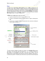
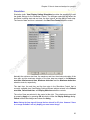
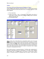
1
ic at io ns S YSTEM S CIENCE A PPLICATIONS , I N C. pp l Environmental Analysis System Sy st em Sc ie n ce A EASy User Manual Version 2005a System Science Applications, Inc. PO BOX 121 Pacific Palisades, CA 90272 www.runeasy.com ic at io ns C OPYRI GHT S Copyrights 2001-2005 System Science Applications, Inc. pp l All rights reserved. ie n ce A Information in this document is subject to change without notice. The materials, content, services and software in this publication are the protected copyright material and the intellectual property of System Science Applications, Inc. unless otherwise noted. No portion of the information contained on this publication may be reproduced without the written consent of System Science Applications, Inc. Sy st em Sc System Science Applications, Inc. PO BOX 121 Pacific Palisades, CA 90272 Tel: 1-800-RUN-EASY Fax: 1-310-123-4567 [email protected] ic at io ns A pp l A BOUT EAS Y ce PRODUCT HIGHLIGHTS st em Sc ie n EASy is an advanced GIS with the capability to view, analyze and store diverse types of environmental data. EASy has been successfully used in a wide range of applications from resource management and oceanography, to pollution studies and coastal monitoring. Unlike other GIS software, EASy has been specifically designed to display data utilizing time, depth and geo-spatial information. This dynamic 3-D capability is vital for studying marine and terrestrial environments with their complex horizontal and vertical structures. Sy EASy's capabilities provide scientists, resource managers, companies and educators with the tools to better interpret and communicate their ideas. Experienced teams work in collaboration with users, customizing EASy to meet needs rapidly and affordably without expensive training. EASy's use in an expanding arena of projects is a testament to its versatility and the experience of our personnel. st em Sy Sc ce ie n A pp l ic at io ns OF ic at io ns T ABLE C ON TENT S pp l Welcome to Easy...........................................................................................................1 Overview: EASy Shortcut guide...................................................................................3 Using this Guide .............................................................................................3 A The two basic operating modes in EASy ........................................................4 A key for viewing or controlling the display data in the project file...................5 ce Building a Project............................................................................................6 ie n Chapter 1: Getting Started............................................................................................7 The EASy Environment ..................................................................................7 About Main menu ...........................................................................................9 Sc Using Toolbar ...............................................................................................10 st em Using Screen cursor commands...................................................................12 Using the File menu......................................................................................13 Chapter 2: How to view and analyze in a project ......................................................15 Using the View menu ..............................................................................................15 About View menu .........................................................................................15 Sy Using Display Settings..................................................................................17 About Display Settings.................................................................17 Birdseye.......................................................................................18 Categories (station data)..............................................................20 Categories (imagery) ...................................................................23 Plots.............................................................................................26 Scenes.........................................................................................30 Settings........................................................................................32 Services.......................................................................................34 Simulation ....................................................................................35 Using Data Graphics ....................................................................................36 About Data Graphics....................................................................36 Plotting data.................................................................................37 About plotting data in EASy .........................................................37 Contours ......................................................................................38 Images.........................................................................................40 Plots.............................................................................................42 Stations........................................................................................43 i ic at io ns Table of Contents Vectors ........................................................................................45 Using Overlays & Overlay sets .....................................................................46 Overlays ......................................................................................46 Using Spatial extents....................................................................................49 pp l Spatial extents .............................................................................49 Using Color Processing ................................................................................51 Color Processing..........................................................................51 A Using GIS options & GIS window .................................................................52 ce GIS options ..................................................................................52 Right clicking on a base or an object to call Ezshape Attributes ......................................................................................................................................56 Right clicking on shape to browse images or audio......................59 ie n Using Image Attributes .................................................................................61 Image Attributes...........................................................................61 Sc Using Legend ...............................................................................................62 Legend.........................................................................................62 Using Palette ................................................................................................63 st em Introduction to the Palette tool......................................................63 Components of the Palette tool dialog..........................................65 Manipulating Existing Palette Posts .............................................69 Using controls in Palette Advanced mode....................................71 Sy Using Statistics .............................................................................................73 Statistics ......................................................................................73 Using Query Settings & Query Results .........................................................74 Query settings..............................................................................74 Query Results ..............................................................................76 Using the Zoom menu .............................................................................................77 Zoom menu ..................................................................................................77 Using the Process menu .........................................................................................79 Browse .........................................................................................................79 Capture Data ................................................................................................82 Simulation Control ........................................................................................85 Chapter 3: How to build or modify a project .............................................................89 Creating a new project..................................................................................89 Using the File Menu......................................................................................90 Services.......................................................................................90 Configuring Services ...................................................90 Import ..........................................................................................93 ii ic at io ns Table of Contents About Import................................................................93 Images ........................................................................94 Preparation for Importing Imagery (Images) ................94 Import a Single Image .................................................97 pp l Import Images from a local directory ...........................99 Importing Images from the Internet............................101 Sensor .......................................................................................104 A Sensor Polling............................................................................104 ce Using the Edit menu ...................................................................................106 Using Database Wizard .............................................................106 About Database Wizard ............................................106 ie n Database Wizard Step 1 - Virtual database files........107 Database Wizard Step 2 - Source File & Connection 109 Database Wizard Step 3 - Measurement name (type)112 Sy st em Sc Database Wizard Step 4 - Measurement value .........114 Database Wizard Step 5 - Measurement units ..........118 Database Wizard Step 6 - Depth ...............................121 Database Wizard Step 7 - Latitude............................124 Database Wizard Step 8 - Longitude.........................127 Database Wizard Step 9 - Station data......................130 Database Wizard Step 10 - Time...............................133 Database Wizard - Finish ..........................................136 Editing Shapes...........................................................................138 Editing Shapes ..........................................................138 Editing Arcshape options...........................................139 Editing Group forms ..................................................139 Editing Member forms ...............................................142 Chapter 4: How to export in a project ......................................................................145 About Export...............................................................................................145 Exporting as an Image................................................................................146 Exporting a Copy ........................................................................................146 Exporting Services......................................................................................147 Exporting Measurement data......................................................................148 Exporting Measurements............................................................................148 Exporting from a selected (clicked) station..................................................150 Chapter 5: How to print in EASy ..............................................................................153 Printing .......................................................................................................153 iii ic at io ns Table of Contents Printing multiple plots onto a page..............................................................155 Chapter 6: EASy reference topics............................................................................157 About Reference Topics .............................................................................157 pp l EASy Services............................................................................................158 List of Selectable EASy Services ................................................................158 Description of Services files *.dll.................................................................160 A EASy Project Files......................................................................................162 ce List of EASy Project Files ...........................................................................162 Databases in EASy.....................................................................................163 About Databases in EASy..........................................................163 ie n List of Databases in EASy..........................................................164 Project Measurement Database.................................................165 About Project Measurement Database ......................165 Sc Tables........................................................................................166 Overview of Project Measurement Database Tables .166 st em List of Project Measurement Database Tables ..........168 Relationships .............................................................................171 Overview of Relational Database ..............................171 Sy Relationships in the Project Measurement Database Tables .........................................................................................................................172 Project GIS Database ................................................................175 About Project GIS Database .....................................175 EASy System Database.............................................................176 About EASy System Database..................................176 Index ..........................................................................................................................177 iv ic at io ns Welcome to Easy Sy st em Sc ie n ce A pp l EASy (Environmental Analysis System) is a geographic information system that is specifically designed for marine and coastal applications; it is powerful yet easy to use (www.RunEASy.com). It runs under Windows operating systems upon PC desktops and upon PC servers. The power of the software is based upon the GIS’s capacity to integrate diverse types of environmental information and models within a 4 dimensional context of space and time. Its power is also based upon the incorporation of interfaces to automate the process of updating information on a server. Components of the geographical information system. The figure also shows the modes of operation, the "Netview" for serving information interactively over the internet and the desktop for the project development 1 st em Sy Sc ce ie n A pp l ic at io ns ic at io ns Overview: EASy Shortcut guide Using this Guide pp l The major aim of this guide is to provide you a convenient starting point to work your way around EASy. EASy has a diverse number of functions and operations which are available for use for any of your projects, and this guide provides a quick reference for them looking up. ce A The design of this guide is to allow you to begin your new project or an existing project every time or at any time from this guide, and call up EASy functions easily to satisfy your project’s needs. ie n Three topics underlie this shortcut guide: 1. The two basic operating modes in EASy; 2. A key for viewing or controlling the display data; and Sc 3. Building a project st em "The two basic operating modes in EASy" gives you an overview of the two modes of operation in EASy, allowing you to quickly carry out any of the 2 modes in a project. Sy "A key for viewing or controlling the display data" outlines the tools (with their shortcut paths) that EASy provides to display or control data in your project. When you are unsure what you may want to do, always start out from this page for ideas and functionalities. "Building a project" provides a roadmap of how you can start a new project from scratch. Beginning your own new project becomes a simple process with this quick roadmap. Always check this topic if you want to do additional materials to your project. With this guide, it is hoped that you can use EASy with ease, and EASy can be a powerful tool for your research needs. 3 Sy st em Sc ie n ce A pp l The two basic operating modes in EASy ic at io ns EASy User Manual 4 ic at io ns Overview: EASy Shortcut guide Sy st em Sc ie n ce A pp l A key for viewing or controlling the display data in the project file 5 ic at io ns EASy User Manual Sy st em Sc ie n ce A pp l Building a Project 6 ic at io ns Chapter 1: Getting Started The EASy Environment Sy st em Sc ie n ce A pp l When EASy is run, a map display of some area on the globe will come up together with an overlaid latitude/longitude scale grid with perhaps some additional blank plot windows depending on the particular default project that was last run. A typical view of the start up screen and the EASy working environment is depicted in the figure below. EASy’s graphical user interface is comprised of several components. The Main Menu and Toolbar provide a user-friendly, means of interacting with the software, linking to and acquiring data, altering settings and views of data, and running application processes. The Messaging Panel, Status Bar and Main Output Window provide users with graphical outputs from and associated textual information about procedures undertaken. These 3 elements are now discussed in further detail. 7 ic at io ns EASy User Manual Messaging Panel and the Status-bar A pp l Information regarding the outcome of operations on data and other such systemrelated feedback is returned by EASy in the Messaging Panel, located at the bottom left of the screen. Depth at the location of the mouse pointer in meters. The distance and orientation of user-defined transect lines in nautical miles and degrees north respectively. System clock time st em The location of the mouse pointer in latitude and longitude coordinates (expressed as degrees: minutes: seconds). Sc ie n ce The Status Bar on the opposite side provides further useful information to users. Progressing from left to right one has: Operation mode Numeric keypad activation status Sy Main Output Window The results of data integration and computation processes undertaken in EASy applications are visualised in a geographical context within the main output window. Spatial data are typically rendered as false color imagery and contours in the horizontal domain, and as vertical contours and depth profile plots along transects and at point locations respectively. The main output window is also where the temporal evolution of spatial data and point location measurements, represented as time series plots and XY graphs of data variables, is observed. The content and precise form that these views take are highly customizable, allowing users to easily choose between plot types, views of actual sampled and simulated data stations, and the level of detail of bathymetric, geographical and associated descriptive textual information displayed via Screen Cursor Commands. 8 ic at io ns Chapter 1: Getting Started About Main menu ce View - display information, create and customize graphical displays, submit spatial queries and raster statistical analysis Zoom - control location and scale of base map Process - choose means of viewing time series—by raster browser, by simulation control panel- or store time series as a sequence of binary files st em Edit - link project to EASy databases or import fields from external database, edit shapefile attributes ie n File - passing information into and out of projects e.g. creating a new project, opening saving changes, opening, importing, exporting, printing Sc A pp l The Main menu contains the key operations for the program including (from left to right): Help - view help file Sy 9 ic at io ns EASy User Manual Using Toolbar pp l Main Toolbar ie n ce A Situated near the top left of the application window and beneath EASy’s pulldown menu system, the Main Toolbar (shown above) provides shortcuts to a range of core operations that users are likely to perform routinely in EASy. These include the opening of a new project file, saving of the current project configuration, printing of screen output, zooming functions, activation of data polling, and acquisition of online help information for EASy. A description of each of the toolbar buttons now follows. Most functions supported by these toolbar shortcuts can also be accessed via the EASy menu system and hot-key combinations. Where available these are indicated for the corresponding item. Sc Note: The main toolbar generally will appear on screen by default, however, this feature is customisable. If deactivated, simply toggle the MAIN TOOLBAR list item of the VIEW menu to on (simply highlight and click on this element to add the checkmark and activate the toolbar appear). st em New button: allows users to setup a new EASy project application. Open a project and replaces the on-screen EASy application with one selected by the user from a pop-up dialogue box with listed project files (.prj file extension). ctrl-O . Sy Menu and hotkey equivalent: /FILE/OPEN Save all currently selected display options and other project configuration information (e.g., map view, plots, contours, palette colors, etc.) in an updated .prj file of the same name, thus replacing the existing project file. Menu and hotkey equivalent: /FILE/SAVE ctrl-S . Print graphics from the main output window on a designated printer via a standard Windows print dialogue box. Menu and hotkey equivalent: /FILE/PRINT ctrl-P . Define a new screen view epicenter. Clicking on this shortcut results in a red cross-hair appearing on screen at the position of the current view epicenter. Move the mouse cursor to the preferred location and left-click to place the new epicenter; the screen view will shift accordingly. Menu and hotkey equivalent: /ZOOM/ZOOM CENTER 10 ctrl-Z . ic at io ns Chapter 1: Getting Started Zoom in by a fixed scaling interval. Magnify and focus on particular areas or features of interest. Menu and hotkey equivalent: /ZOOM/ZOOM IN ctrl-Down . pp l Tip: Hone in and magnify particular areas or features of interest by combined use of the ZOOM CENTER and ZOOM IN tools. ce A Zoom out by a fixed scaling interval for views having broader geographic coverage. Menu and hotkey equivalent: /ZOOM/ZOOM OUT ctrl-Up . st em Sc ie n Window into and focus on specific areas of interest by a custom amount. Press the Zoom Window button, left-click to anchor the uppermost edge of the rectangle, drag the mouse cursor to resize the viewing window over the area or feature of interest, and then release the mouse button for the magnification to take effect. Menu and hotkey equivalent: /ZOOM/ZOOM WINDOW ctrl-W . Refresh screen. Click the Refresh button to update the screen view. Press this button to activate EASy’s remote data polling Sy Poll Button. functionality. Note: Data sources (local/network drive, anonymous ftp site, remote sensor) to be accessed must previously have been specified and appropriate configuration settings made or Run/ Stop Button. simulation. Press this button to start and stop EASy’s Help Button. Provides the user with access to context sensitive online help on all aspects of the EASy software system and associated application development topics. Menu and hotkey equivalent: /HELP/ HELP TOPICS ctrl-A. About EASy. Clicking this button pulls up a window displaying current EASy version number and release date information together with related software copyright information. Menu and hotkey equivalent: /HELP/ ABOUT shift-M. 11 ic at io ns EASy User Manual Using Screen cursor commands Besides the ability to select menu items, enter information, and display screen tips, the mouse cursor can be used to sample many of the objects displayed on the screen: pp l If the mouse command does not yield the desired information, either the format of the object is not compatible or the project requires editing. A 1. a left-click on window then left-click-drag to select region for windowing and statistics ce 2. a single left-click on bathymetric contours yields a depth estimate in the status bar ie n 3. a control-(left-click) on a raster image yields a value for that variable in the status bar 4. a double left-click on a raster image that is a layer of a 3-dimensional field yields a plot of the variable as a function of depth Sy st em Sc 5. a double left-click on a Arcshape or Ezshape will display a form containing its attributes 6. a double left-click on a station yields a form containing a list of measurements, and buttons for plotting depth profiles and time series, exporting selected measurements and a button for linking to related sites 7. a right click anywhere displays a list of Menu commands 8. a shift-click-drag yields a transect (whose distance and heading are indicated in status window) yields: 12 a depth profile if bathymetry is displayed and when View/Data Graphics/Plots/Depth profile is selected pixel values of an underlying 2-dimensional raster image a curtain plot of underlying 3-dimensional field ic at io ns Chapter 1: Getting Started Using the File menu Using the File Menu Sy st em Sc ie n ce A pp l Under the File menu, you can: 13 st em Sy Sc ce ie n A pp l ic at io ns ic at io ns Chapter 2: How to view and analyze in a project Using the View menu About View menu pp l The View menu allows the user to modify the project screen display and select between different available measurement types and forms of data output. The menu is partitioned into four sections, A 1) The first deals with customization of the graphical user interface via toggling of various toolbar shortcut and status bar elements. ce 2) The second group of menu items pertains to the visualization of project data and geographical information in the active EASy application. ie n 3) The third group of items performs a variety of functions mainly related to the configuration for displaying data, the addition of new GIS objects, and the reporting of information from data. Sy st em Sc 4) The last group allows users to extract information quickly from the displayed data with simple, quantitative statistical representations In the View menu, there are several key features: Tabbed menu to choose and customize graphics Menu to choose variables and associated graphics 15 Options window to view vector objects Custom grouping of vector objects Window to choose stations and associated variables ic at io ns EASy User Manual A pp l Note & Tip: Changes made to the active project view will only be maintained for the duration of the current session unless the project file is saved (main toolbar Save shortcut or File/Save or /Save As menu item). Use Save As if the original .prj project file must not to be overwritten. Main Toolbar: Clicking on this list item toggles on (checked) or off the Main Toolbar of EASy . This toolbar provides shortcuts to a range of core operations that users are likely to perform routinely. These include the opening of a new project file, saving of the current project configuration, printing of screen output, zooming functions, activation of data polling, and acquisition of online help information for EASy (See, Using Toolbar for further details). Once removed, functions supported by toolbar shortcuts must be accessed via the EASy menu system. Status Bar: Use this toggle to control whether the Status Bar with associated information will be displayed in the EASy program window. Sy st em Sc ie n ce The functions of the first two items on the View menu is outlined below: 16 ic at io ns Chapter 2: How to view and analyze in a project Using Display Settings About Display Settings ie n ce A pp l The Display Settings (path: View/Display Settings) dialog allows users to configure a number of data display options, and to turn on or off items that are displayed on the screen. Birdseye Categories (Station data, and Imagery) Plots Scenes Settings (for the global EASy environment) Services Simulation Sy st em 1) 2) 3) 4) 5) 6) 7) Sc This dialog has the following seven tabs, each performing a unique set of operations: 17 ic at io ns EASy User Manual Birdseye Sy st em Sc ie n ce A pp l The Birdseye feature (path: View/ Display Settings/ Birdseye) gives users a birdseye view of the area using user-defined scale. The map also displays the zoom center currently set. To select the Birdseye options, select the View menu, and press Display Settings. Under this menu select the Birdseye tab to change your specifications. EASy provides users with the opportunity to define the size, shape and location of the Birdseye view, depending on your project needs. Not only can you set the size of your window, but you can also add a new "birdseye" view by pressing Add, which will add a new birdseye (e.g. Birdseye-2) view to your choices. If you do not want to display the birdseye at all, simply press Delete on all your views and click Apply. Within the Birdseye tab users can edit the size and location of the window by editing the window box. To adjust the location of your Birdseye window within EASy, use the 18 ic at io ns Chapter 2: How to view and analyze in a project pp l first two boxes of the Window control. The first number controls the windows location horizontally from left to right. The default is set at 0, i.e. on the left. To move the window to the right, increase the number to your preference (up to 988 which is all the way to the right). Similarly, the next button dictates the location of the window vertically, where 0 = top of the screen, 623 = the bottom of the screen. A The parameters of the map can be modified to suit user requirements. The last two buttons of the Window control adjust the height and width of the window itself. The height can range from 10 to 510, whilst the width can range from 10 to 324. ie n ce Note: the map itself will remain the same scale regardless of height or width. Modifying the height and the width simply allows users to adjust the extent of the view and the given area. To adjust the Center of your birdseye, you can enter the latitude and longitude, or use the scroll button to select the center by hand. st em Sc Note: Changing the zoom center on the base map does not alter the zoom center in the Birdseye view. It will simply display the zoom center locator at another location in your Birdseye view. Sy Users also have the option to adjust the scaling of the map to fit more or less into the view depending on the focus they require. You can specify the number of feet per pixel by entering a number in manually or by scrolling up and down using the cursor. The maximum range allowed is 599999 and will be extremely zoomed out. The zoom will vary from project to project accordingly depending on your preference. 19 ic at io ns EASy User Manual Categories (station data) Sy st em Sc ie n ce A pp l The Categories (path: View/Display Settings/Categories) dialog provides the tools to edit the legends of imagery and station data. In this example, we describe the scaling of the size legend for blob plots and scaling of the color legend and pixel values for false color imagery of station data. The variable (here "temperature") is chosen in the selection window, and it is then available for editing by pressing the Edit button. Its name in the Category table of the EASy database is then displayed in the Category window, and its properties are then displayed in 3 underlying selection controls. These classifications are found in the Image Format table (Image Format Name field), the Import table (Import Name field), and the Measurement Type table (Measurement Name field) of the project database (See, List of Project Database Tables for a description of the tables). 20 ic at io ns Chapter 2: How to view and analyze in a project A pp l The image’s legend can be turned on and off by pressing the Legend button, and the format of the legend can be modified by entering values in the Values and Height selection controls. Select from Type whether the measurement is a measurement, the depth in ocean, or the elevation on land. In addition, users will see a display of the units of the measurement in Units and the C standard format code for its values in Fmt (e.g. here %6.2f represents 6 characters with 2 decimal places for a floating point number). Sc ie n ce In EASy, colors and value of pixels in images as well as the diameter of blobs and the co-ordinates of vectors are based upon a quasi, 8-bit scale, in which these quantitative properties are sorted into 235 bins whose counts range from 0 to 235. This scale is then used to create legends for image colors, vectors, and blobs as well as converting quasi-8 bit count of a pixel into a value for the associated measurement. This scale is fixed and is displayed in the dialog as the Color Palette Value text near the bottom. (It is also displayed as a list under both the Pixel/Units button and the count-pixel frequency scroll box under Frequency/Percent button in the Palette (path: View/Palette). The counts from the quasi-8 bit scale are converted to measurement values via a function that is displayed in the Function selection control. Sy st em EASy offers options for linear, exponential, logarithm, and power functions in this selection control. In addition the values for the coefficients are displayed and selected in the Offset, Slope, and Const (Note: this is not used in linear function) selection controls below as is a graph of the function. The Color Palette Value scale is in fact displayed as one abscissa of this graph, and below it is a second abscissa, the Source Pixel Value selection controls. The minimum and maximum values of this control are determined by the range in values of the source measurement. In the case of station measurements this range is always set to a true 8-bit scale of 0 to 255, but in the case of Imagery this scale will vary with the type of processing. When station data is imported into the project database a linear conversion of Color Palette Value (counts) to values in legends is assumed and values for the Offset and Slope coefficients are calculated and entered here and into the corresponding fields of the Measurement Type Table. In addition, the minimum and maximum counts of the Source Pixel Value are set, entered into the "Measurement Minimum" and "Measurement Maximum", fields of the Measurement Type Table. They are set automatically when "Project", "Computed" is entered in the Category Format Field of the Category table of the project database. The function is then graphed. 21 ic at io ns EASy User Manual Sy st em Sc ie n ce A pp l When the coefficients of the conversion function and the Source Pixel Value are entered, the values for the minimum and maximum of measurement values will be displayed in the Physical Minimum and Physical Maximum selection controls. Alternatively, if values for Source Pixels Value and the Physical Minimum and Physical Maximum are selected, then values for Offset and Slope will be determined. These values for coefficients and source pixel values will not be updated when additional data are appended to the database. Thus, new values must be entered using the controls available here. 22 ic at io ns Chapter 2: How to view and analyze in a project Categories (imagery) Sy st em Sc ie n ce A pp l The Categories (path: View/Display Settings/Categories) provides the tools to edit the display of a selected imagery and station data. In this example, we describe the scaling of the color legend and pixel values for a new category of imagery that has been imported using the File/ Import/ Imagery dialog. When a new category of imagery has been successfully imported, the name of the image (from the Measurement Name field of the Measurement Type Table of the project database) is chosen in the selection window, and it is then available for editing by pressing the Edit button. Its classification in the Category table of the EASy database is then displayed in the Category window. Its properties are then displayed in the 3 underlying windows, 23 ic at io ns EASy User Manual A pp l Image Format and Import Type are fields in the Category table, and Measurement Type is a field in the Measurement Type Table. The image’s legend can be turned on and off by pressing the Legend button and the format of the legend can be modified by entering values in the Values and Height selection controls. You can select from Type whether the measurement is a measurement (imagery and stations), the depth in ocean, or the elevation on land. In addition you will see a display of the units of the measurement in Units and the C standard format code for its values in Fmt (e.g. here %6.2f represents 6 characters with 2 decimal places for a floating point number). st em Sc ie n ce In the next selection control Function, select the form of the function that transforms the pixel counts of the image file, here called the source pixels to the values of the measurement. Options include linear, exponential, logarithmic, and power. The minimum and maximum counts for the source pixels are selected in Source Pixel selection controls at the abscissa of the graph of the function. On the other hand values for the coefficients of these functions are entered in the controls Offset, Slope, and Constant. Once minimum and maximum counts for the source pixels and the values for Offset, slope, and Constant (not a coefficient in linear function) and are selected, a graph of the relationship is plotted, and the maximum and minimum values for the measurement are displayed in the Physical Minimum and Maximum selection controls. Sy Alternatively, the relationship between source pixel count and measurement value can also be uniquely determined by entering values for the lower and upper limits of measurement values and the lower and upper limits of the source pixel counts. The header of the image file often contains information that describes this function. This information may include the form of the function, the value of its coefficients, the range of source pixel counts, the range of measurement values, and the units of the measurements. The content of the header of an image that is displayed is displayed in the Image Attributes File dialog (path: View/ Image Attributes). It is helpful to consider the conversion of source pixel counts to measurement values as a 2- step process. 1) In the first step the counts of pixels in the image file, the Source Pixels, are transformed into Color Palette counts by binning them into a quasi-8 bit color scale in which pixel counts vary from 0 to 235. This color scale, which is displayed in the abscissa of the graph that is labeled Color Palette, map 1:1 to the pixel counts listed from 10 to 245 that is displayed in the Palette dialog (path: View/Palette). It is the distribution of pixel counts in the Color Palette that determines the distribution 24 ic at io ns Chapter 2: How to view and analyze in a project of colors in the image. The conversion of Source Pixel counts to Color Palette counts is done automatically when one enters the minimum and maximum values of the source pixels in the Source Pixel selection controls at the bottom of the dialog. Sy st em Sc ie n ce A pp l 2) In the second step the counts of pixels scaled to the Color Palette are transformed into the measurement values of the pixels. Values for defining the relationship between source pixel counts and measurement values found in the of the image file header can also be entered into the Measurement Type Table of the project database. In this table the "Measurement Minimum" and "Measurement Maximum" of an image record contains the Minimum and Maximum counts of the Source Pixels. The slope and offset fields are clearly labeled in the table. If entered in the measurement type table, these parameters will appear in the Categories controls. 25 ic at io ns EASy User Manual Plots A pp l The Plots (Path: View/ Display Settings/Plots) option in EASy provides users with the ability to add, modify or delete X-Y graphs. The plots will also change through time during a simulation, displaying the relevant data for that time period. The plots created with this dialog display all station data found in the project database. The dialog is just one of three means of creating plots. Alternatively you can create plots using the Edit/ Project dialog or through the EASy VB API. In EASy there are three types of plots are offered: ce 1) xy plots of measurement value at a give location vs. time, 2) xy plots of measurement values at a give location vs. depth or altitude plots, and Sy st em Sc ie n 3) a plan view or computed images of measurement value (vectors or scalars) at a given depth or altitude The plots currently available for display are viewed in the Available Plots window (see above). They are also listed in the project file, *.prj. To modify the order your plots appear, use the Arrows to the right to move from top to bottom. This just enables users to group together plots which are commonly related by a plot type etc., or however they see fit. To delete a plot, select the one you want to remove and press 26 ic at io ns Chapter 2: How to view and analyze in a project pp l Delete. To create a new plot, press the Add button. The name of the new plot is entered in the Plot Name entry field (e.g. TemperatureFcol Vs Depth). Once you have chosen your name, you can select one of the three plot types you wish to create using the Plot Type pull down (e.g. measurement variable against depth). ce A Note: If the measurement of interest does not appear, to troubleshoot it, you must enter it as a record in the Category Table in your project database under the EASy directory project folder. Minimally, the fields for "Category Name", "Measurement Name", and "Format Type", must be entered into the table. In addition the creation of plots from station data requires that the "Format Type" be either "Project" or "Computed" (See Entering a new category in the project for details.) ie n The 2 selection controls labeled Station and Voyage provide additional options for creating plots. The Station selection control offers 3 options; Sc Station Plots - any station can be selected for display of plots of measurement value vs. depth or time. st em Measurement Plots - the data from all stations will be displayed on an individual plot of measurement value vs. depth or time; finally, if one selects Individual stations - plots for only those stations will be available. Sy The Voyage selection control offers options for creating plots for types of data such as drifters or buoys that are not stored in formats other than the project database. Configuring the axis The controls for the x-axis and y-axis are directly below the Station/Voyage controls. Here users can edit the scaling, modify the range and label the axis accordingly. Note: the boxes will change depending on whether you select a plot for variable versus depth, a false color image plot or through time. The information displayed here will depend upon the plot type: I). Variable versus Depth If you decide to plot a variable versus depth, you can do one of two things; 1). Run your plot using all the depth information plotted together, or 2). You can make plots displaying user-defined depth-strata(s). To do so, select the 27 ic at io ns EASy User Manual minimum and maximum depths for your new strata using the min/max(m) control. pp l Note: Depth profiles will be displayed in meters by default. If you require scaling to be in feet, you will need to change your units to English using Display Settings/Settings tab. In doing so, however, you will modify the global settings of the entire project, thereby converting all your units into English. ie n II). Variable versus Time ce A EASy will access your project database and compute the information, producing an output of the selected data. When using this plot type, the y-axis is automatically labeled "depth" for a profile plot. Sc If you select a variable versus time plot, the x-axis (i.e. the bottom box) will automatically be labeled "time," since it is time series. The measurement name and its corresponding units should be displayed in the axis labels automatically when using this type of plot. st em III). False Color Images Sy By choosing to plot a false color image, the panels will automatically change to become Depth and Image (see below). Here, EASy gives you the ability to create a false color image based on your station data e.g. Conductivity. Select the Scale of the x-axis and y-axis with the x-axis, y-axis selection controls, and enter the measurement units of the y-axis in the text box between the two selection controls. The y-axis is automatically labeled as "Depth" (as in the above figure) for a profile plot or with the measurement name and its units for a time series plot. On the other hand the x-axis is automatically labeled "Time" for a time series or with the measurement name and its units if the plot is a profile. 28 ic at io ns Chapter 2: How to view and analyze in a project When EASy computes your image, it plot a false color image based the station data values within your database. The reach determines the size of the stations that will be sampled. By increasing the reach you will amalgamate any stations that fall within the same area. pp l Modifying the resolution of your image will determine the size of the pixels within your image. A Reserved station plots Sy st em Sc ie n ce Finally, the maximum number of xy plots that can be displayed at one time is selected in the Reserved station plots selection control. We note that all plots and images are updated at each step during the display of a time series with the simulation control panel. In the case of photo images after the execution of the time step the last image recorded. 29 ic at io ns EASy User Manual Scenes Scenes (path: View/Display Settings/Scenes) are groups of data, associated graphics and controls that are pre-selected in order to present coherent theme. pp l By right-clicking on the base map, users can view the scenes currently displayed or available to display from the scenes menu. Sy st em Sc ie n ce A To change the order they appear, highlight the scene you want to move and press either the up arrow to move it up the order, or alternatively down to move it downwards. This simply allows the user to adjust the order scenes are listed when right-clicking on the base map. A new scene is first named by pressing the Add button and then entering the name in the text window. A scene can be removed by first selecting it, and then pressing the 30 ic at io ns Chapter 2: How to view and analyze in a project Remove button. Finally, the settings for a scene can be cleared by selecting the scene and then pressing the Update button. ce A pp l When the buttons to the left of the main selection control are pressed, the options associated with the name of these buttons are displayed in the selection control. If the box to the right of the button is checked, the selections for the scene that has been selected will be implemented. If not checked, the selections for the scene that was previously selected will be implemented. The function of the buttons down the list goes as follows: ie n 1) Blob - allows you to select the scenes’ time series for blobs and stations that will be displayed when the Simulation Control is running the time series. Sc 2) Browse - allows you to select the imagery that will be displayed in the scenes’ Image Browser. 3) Contour - allows you to select the data that will be displayed as contours when the Simulation Control is run. st em 4) Extents - allows you to select the spatial boundary of the home zoom screen. 5) Model - allows you to select the imagery that will be displayed when the Simulation Control runs. 6) Overlays - allows you to select the scenes’ Overlays and Overlay sets from the list found in View/Overlays. Sy 7) Settings - allows you to select the settings (e.g. legends, compass, projection) that will be displayed in the scene. 8) Time - allows you to select start time, end time, and time-step for that scenes’ Simulation Control. 9) XY-Plots - allows you to select the XY plots that will be displayed from the list found in View/Data Graphics/Plots. Tip: To display a particular defined scene, simply right-click on the base map, point your mouse to Scenes and select options from the pull-right menu. And generally, the following tips are noteworthy o Add scenes as the final step in creating projects o Check scene definitions after adding or removing project data o Test each new scene (e.g. view and hide) before saving project o Select a scene (not ‘None’) for NetViewer 31 ic at io ns EASy User Manual Settings Sy st em Sc ie n ce A pp l The Settings tab (path: View/Display Settings/Settings) provides global controls over the base map display. The functions and buttons available in the settings tab are: The Units box controls the global settings for units used. Distances are displayed in either metric or English units. The format of latitude and longitude is selected in the Lat/Lon selection control. At present, EASy has four formats of lat/long. The settings menu controls the display of Legends. Check boxes for Birdseye, Credits, Measurement Legends, Compass, and Scale Bar can be checked appropriately to display or remove legends on screen. 32 ic at io ns Chapter 2: How to view and analyze in a project The Projection of the base map may be in Mercator, Lambert conformal, or Arc Grid lines and grid labels can be displayed or hidden by checking the boxes to the left of Grid Lines and Grid Label buttons. The color of the grid lines and labels are selected by pressing the buttons pp l The Mouse Wheel box provides controls for performance, Cycle, and Wheel limit value The Image Vectors box provides selection controls for the length for the arrow, ce A Arrow length, the size of the arrow head, Arrow head size, and the number and position of the limbs of the arrow head, Arrow head style. The color of the arrow is selected by pressing the Color button. The size, shape, and color of the arrow are displayed in the accompanying figure The Display Size box provides controls for selecting the global settings for ie n items displayed on screen such as, the blob size of spatial extents. Increase or decrease the size of displayed items with the arrows buttons. o The text size for all identifications or Ids (e.g. stations) is selected with Sc Text size scale o The Line Filter control allows adjusting the balance between imagery st em load up speed and resolution. The control can aggregate line segments of imagery to achieve a faster loading speed, but the drawback is the resolution will be decreased. The default is set to 1, which means no aggregation and maintains the highest possible resolution of your imagery The Snap box: function not yet available Sy The Background Colors box allows you to select the colors of the Screen by pressing the Screen button and the colors of xy plots by pressing the XY Plots button 33 ic at io ns EASy User Manual Services Sy st em Sc ie n ce A pp l The Services tab (path: View/ Display Settings/ Services) provides users with the means of displaying Ezshapes and other shapes such as DXF files and WDB files such as bathymetry, coastline, and elevation. In order to display a service, users must have already pre-selected their service or services using the File/Services menu. If your required service is not displayed, or you want to create a service, you must go to the File/Services menu. The files that have been imported into the project are displayed and can be selected in the large text box. The selected file are then be displayed the Display box. Selected polygons are filled by checking Solid fill, and text labels are displayed (if available) by checking IDs. Finally, the distance that a line will be drawn to connect adjacent loci of a polyline is selected with the Reach selection control and the color of the line will be selected from the Palette selection control. 34 ic at io ns Chapter 2: How to view and analyze in a project Simulation Sy st em Sc ie n ce A pp l Simulation (path: View/ Display Setting/ Simulation) provides the opportunity to edit the global settings for the Simulation Control. The changes made here will affect the simulation including start and end time, the time interval, and the delta of each step. The format of date and time is selected in the Date/Time Format selection control. Naturally the minimum start time, the maximum end time, the minimum duration of the time step, and the maximum duration of the time step are entered in the Minimum start time, Maximum end time, Minimum delta time and the Maximum delta time selection controls, respectively. The start time, the end time and the time step in the Simulation Control that is currently available (see View/Display Settings/Scenes tab)are entered in the Default start time, Default end time, and Display delta time selection controls. The units of time are selected in the control at the right. The selections are executed by pressing Apply or by pressing OK which also closes the Display Settings dialog. Cancel cancels the changes and closes the dialog. Note: Altering the time step will change the time interval for XY plots. However if there is no image available it will only display your most recent image. 35 ic at io ns EASy User Manual Using Data Graphics About Data Graphics ce A pp l The Data Graphics (path: View/Data Graphics) control allows users to display data in various presentations, such as in XY-plots or in false color images. Sy st em Sc ie n Refer to the topic, About plotting data in EASy for a description of the display types. The control also provides the selection of particular data sets to display through the filtering options of the Sensors tab and the Voyages tab. 36 ic at io ns Chapter 2: How to view and analyze in a project Plotting data About plotting data in EASy In EASy, data may be viewed as pp l 1) Contours, 2) Images, 3) Stations, A 4) Vectors, and ce 5) Plots (or XY-Plots). Sc ie n Variables available to be viewed via a given graphic are listed in the text box for the tabs found at View/Data Graphics/"tab". st em If a variable in the project files is not listed, select View/Display Settings/Categories to see if it has been entered in the project database and thus available for graphical display. Sy If not listed in Categories, the variable must be first entered in the Measurement table, Image Format, and Category tables of the project database. 37 ic at io ns EASy User Manual Contours Sy st em Sc ie n ce A pp l The Contours (path: View/Data Graphics/Contours tab) dialog lists all data variables (in-situ or remotely sensed measurements and computed values) for which output as a contour plot has been defined in the active application’s project file. The contours may be calculated for a specified variable at a single depth or for the average, minimum or maximum of a variable over a pre-specified depth range. Note: Here we refer to contouring of spatial data in the horizontal rather than vertical dimension. Available vertical contour plot outputs are listed under Plots (path: View/Data Graphics/Plots) tab of the Data Graphics dialog box. Click on and highlight the list item of interest, and press the Apply or OK buttons to plot contours of the selected data variable. Only one variable at a time can be plotted as a contour plot. However, it is possible to undertake spatial data comparisons by plotting a second variable of interest as a false color image. EASy supports the overlaying of contour and false color image plots or indeed any other defined plot types for a given application (e.g. vector, XY plots etc). 38 ic at io ns Chapter 2: How to view and analyze in a project Although selection of data variables for plotting via the Contours dialog can occur at any time, EASy will only plot contours on screen if the project is being run and adequate data exists. If the latter is not true, then the following status message will appear in the EASy Messaging Panel: pp l "No station data defined for computing horizontal contours at current simulation time". Sy st em Sc ie n ce A Note: W hen interpreting contour output, users should bear in mind that what is actually being observed is a field of estimated data values based of spatial interpolations from available empirical measurements. Particular care is required when dealing with sparse spatial data matrices and in the vicinity of measurement boundary zones or in areas with complex coastline geography. Parameters controlling the implementation of contouring algorithms in EASy are defined in the active application’s project file (ezprgrmvb.dat). 39 ic at io ns EASy User Manual Images Sy st em Sc ie n ce A pp l The Images (path: View/Data Graphics/Images tab) dialog allows the selection of data variables for output as false color image plots. All variables (in-situ or remotely sensed measurements and computed values) for which a horizontal measurement field exists can be plotted in this manner. Users can also select images to be displayed during a time series that is called from either the Start/ Stop button or the Simulation Control panel. Variables for which false color plotting has been defined for the active EASy application are presented in the first list-box field. Simply click on and highlight the list item of interest from the dropdown menu, and press the Apply or OK buttons (the former maintains the dialog on screen whereas the latter clears it). Note & Tip: Only one variable at a time can be plotted as a false color image plot. However, it is possible to undertake spatial data comparisons by overlaying a second variable of interest as a horizontal contour plot. 40 ic at io ns Chapter 2: How to view and analyze in a project pp l Selection of data variables for plotting via the Images dialog can occur at any time. However, with the exception of imagery data viewed in false color via Browse mode, EASy will only plot false color plots on screen if the project is being run and adequate data exists. In the absence of sufficient data, the following status message appears in the EASy Messaging Panel: "No station data defined for computing horizontal contours at current simulation time". ce A EASy permits the superposition of multiple (up to four) false color variable plots and provides a mechanism of generating image composites via the three additional listbox fields and the pull-down selection controls on the right. Three options are available in these pull-down selection controls: Normal: the entire image will be shown. ie n Cutin: only the seaside of the image will be shown. Sc Cutout: only the landside of the image will be shown. This capability is only available when the world coast database is displayed at the same time. st em When the Retain images box is checked, images from the previous time step will be displayed until they are replaced by a current image. The remaining portion of the control window can be ignored. Sy Note: False color plot generation is effectively based on EASy’s contouring algorithms. W hen interpreting false color imagery output, users should bear in mind that what is actually being observed is a field of estimated data values based of spatial interpolations from available empirical measurements. Particular care is required when dealing with sparse spatial data matrices and in the vicinity of measurement boundary zones or in areas with complex coastline geography. Parameters controlling the implementation of contouring algorithms in EASy are defined in the active application’s project file (ezprgrmvb.dat). 41 Plots ic at io ns EASy User Manual The Plots (or XY-Plots, path: View/Data Graphics/Plots tab) dialog allows users to graphically display time series of measurements at point locations, pp l dependencies between data at selected stations, and A vertical structure of data along user defined transects. Sy st em Sc ie n ce The Plots dialog presents the user with a listing of available variables for output. Simply click on and highlight the variable(s) of interest from the list box, and press APPLY or OK to plot the graph(s) in the main output window. It is possible to select and display XY-Plots of multiple variables on screen at the same time. Resulting plot windows can be moved and resized as necessary by the user to optimise views. 42 ic at io ns Chapter 2: How to view and analyze in a project Stations pp l The Stations (path: View/Data Graphics/Stations tab) dialog allows users to specify whether, how and when data stations will be plotted on screen. EASy defines 2 types of data stations: A 1) Environmental stations (ENV) are spatially discrete locations (i.e. having a unique set of coordinates) at which in-situ field measurements have been made and recorded in the main project database (core MS Access .mdb file) Sy st em Sc ie n ce 2) Simulation stations (SIM) are spatially discrete locations within a regular lattice of stations superimposed by EASy for computational purposes. The central dialog window provides a complete listing of project stations with their associated ID’s. Environmental stations appear in green whereas listed simulation stations are black. The scrollbar can be used to browse the list. Users can select sets of stations of either type for display by clicking on individual items in the list. Select the mode of environmental and simulated station display by selecting a suitable entry from the dropdown list in the ENV and SIM fields respectively. 43 ic at io ns EASy User Manual None: if stations should not be displayed, Selected: a subset of stations of a given type (highlighted station list elements) is to be plotted on screen. Active: only stations with data for the current time interval of a project run being displayed. A pp l All: plotting the full complement of stations for the entire duration of the project run irrespective of whether stations possess data at a given time step. Sy st em Sc ie n ce Environmental and simulation stations appear as green and blue dots within the main output window respectively. Check the respective boxes in the ENV and SIM fields if output of station ID numbers is required. 44 ic at io ns Chapter 2: How to view and analyze in a project Vectors pp l The Vector (path: View/Data Graphics/Vectors tab) dialog allows a graphical representation of spatial data comprised of directional and magnitude component as Vector plots. A Variables for which such plots are defined in the project files of the active EASy application are listed in the Vectors tab under the View/Data Graphics menu item. Click on and highlight the list item of interest from the listbox. Press Apply or OK as appropriate to display vector output. Sy st em Sc ie n ce It is only possible to select and display one vector variable field at a time on-screen. However, overlaying of vectors and other plot types is supported. 45 ic at io ns EASy User Manual Using Overlays & Overlay sets Overlays st em Sc ie n ce A pp l The Overlays (path: View/ Overlays) window allows users the options to select and configure shape-files for display on base map. In the figure below, the base map, the Overlays window, and the Legend (to turn on the legend, see Legend) are displayed; any applied changes (by pressing Apply) will be shown correspondingly. Sy The overlays box contains a list of all of the overlays available to the user. Each overlay can be defined using its own individual color scheme defined by you to help you recognize that particular feature. To modify the overlay label, left-click on it to highlight and press Line color or Fill color, or simply double click on the line or fill color boxes. This will automatically display a range of colors to choose from. Select the desired color and press OK. 46 ic at io ns st em Sc ie n ce A pp l Chapter 2: How to view and analyze in a project Sy The Shapes box gives users the option of selecting other vector objects, for instance GIS objects, coastlines and bathymetry. To display an overlay, simply highlight the overlay(s) you want display and press Apply or OK. To remove an overlay, deselect it from the list and press Apply. Since some overlays may overlap (e.g. roads will invariably be on land), EASy gives users the opportunity to modify the Order that overlays appear on-screen using the two arrows on the side. To change the order they appear, highlight the overlay you want to move and press either the Up arrow to move it up the order, or alternatively down to move it downwards. By moving an overlay further towards the top of list, it will be displayed earlier by EASy on the map i.e. the overlay at the top will be displayed first, then the second will be displayed and so on. Note: If you are selecting an overlay and it does not seem to be appearing, make sure that there are no other overlays (such as the country or state map) appearing above your overlay. 47 ic at io ns EASy User Manual There are several display options: Select from the Value type scroll for a category of variables that provides a color scale for the selected shapefile. pp l Select from the Value field scroll for the selected shapefile attribute, which provides a value for selecting a color from the color scale (8 bit). Select the selected shapefile attribute to be displayed with the screentip from the Tooltip field scroll. A Select the diameter of a shapefile point from the Point scroll and set the width of a shapefile line with the Line scroll. ie n ce Select the icons of a selected Overlay or Shape using the Icon scroll or Icon File. Sc Another useful feature available using the Overlay menu gives users the opportunity to create sets of Overlays and Shapes known as an Overlay Set. To create an Overlay Set, press the Add button and enter the name of the new set into the window below the Remove button (Set1). st em Similar to the Overlays themselves, Overlay Sets are ordered using the arrow buttons; the bottom layer listed at the top of the list. Overlay sets can be used to quickly display a specific set of overlays, without having to continually select your overlays manually. Sy Tip: It is good to test each new overlay set (e.g. view and hide) before saving project. To display a defined overlay set, right-click on base map, move over cursor to Overlay, and select from the expanded pull-right menu. 48 ic at io ns Chapter 2: How to view and analyze in a project Using Spatial extents Spatial extents Sy st em Sc ie n ce A pp l Spatial extents (path: View/ Spatial extents) allows the display of stations, and station data on top of a base map graphically with points and blobs. Variables are selected for display from selection control by left-clicking on the category so that a dark blue label is superimposed upon it. A selected variable is removed from display by left-clicking on it a second time. More than one variable can be selected for display. If a variable is not listed it must be added to Category Table in your project database in your project folder under the EASy directory. Several options allow a particular type of data to be displayed: All - displays on the base map all stations sampled in time series; Active - displays on base map stations that were sampled during the time-step; Data - displays on the base map stations where the selected variables were sampled during the time step. Blob - creates a blob at the station where the selected variable was sampled. Blobs are of 5 types: 1. presence/absence, 2. counts (number of samples taken), 3. value (value of the measurement- see legend), 49 ic at io ns EASy User Manual 4. count pie (fraction of number of samples taken for a given variable),& 5. value pie (fraction of value of the measurement contributed by a given variable). A pp l Scale the size of station marks + and the size of blobs with the Count/Value scale selection control, respectively. Global rather than variable-specific control of blob sizes is under Display Sizes section of the View/Display Settings/Setting. ie n ce Adjust the size of the + symbol for the data (variables) selected in the Category selection control above with the Station size selection control, and adjust the width of the line defining a blob with the Station width selection control. Sy st em Sc A blob can be a filled with a color selected from the Fill Color button by pressing the Solid button. The color of the blob’s circumference is selected from the Pen Color. 50 ic at io ns Chapter 2: How to view and analyze in a project Using Color Processing Color Processing pp l Color Processing dialog (path: View/Color Processing) allows the modification of algorithms for scaling image values into Palette entries in EASy. ce A Presently, a 256-color palette is supported by EASy for the display of imagery. Consequently, the image values have to be scaled to fit into a 256-color palette. A user can choose between the processing algorithms used in scaling the image values. First, open up the image you want to display from the Browse mode. Then in the first panel, pick from the 4 available algorithms and experiment the best scaling algorithms to use. Press OK to see if the scaling is satisfactory in bringing specific features etc. Sc ie n Color Processing is particularly useful when a source image has its image values located within a small range of pixel values. Thus when the image is displayed with a default palette, for example, Greyscale, the features of the image may not come up with distinctive colors. The Color Processing option provides the ability to spread out the small range of pixel values, while without modifying the original physical values. st em In the second panel, all the images in a category can be forced to follow the same scaling factors set by the first displayed images. Thus, it is possible to first set the scaling factors for 1 image, view it in the main output window, and then check the "Retain image scaling factors" box to apply to all other images. Sy In the last panel, the image quality and load speed trade-off can be selected. For the highest image quality, enter 1 in the scroll box. For the highest load speed, enter 50. 51 ic at io ns EASy User Manual Using GIS options & GIS window GIS options pp l Like Arcshapes, Ezshapes are geometric objects (i.e. vectors: points, lines, rectangles, ellipses and polygons), developed for EASy, which may or may not be labeled with a name. st em Sc ie n ce A When left-clicked, shapes display an attributes form. An attribute form can be created for a shape consisting of many points and for the each point that forms the shape. Ezshapes attributes are edited and created with the GIS Options dialog, which is displayed by either selecting the menu sequence, View/GIS Options, or right-clicking on a shape and selecting GIS Options. Sy The key modules of this dialog provide the following functions: Fixed image height/width determines the dimensions of the Ezshapes’ Attributes Forms. Stretch image provides a tool used to determine an aspect ratio of an image that is to be displayed in the Attribute Form. Hide shapes allows hiding of one or multiple shapes in the Ezshapes. Raster Mode selection control defaults to copy but may be set at Paint, Invert, And, and None. Ezshape editing is activated by pressing the radio button Display/Edit. The button will now be labeled Edit rather than Display. Press OK. 52 ic at io ns ie n ce A pp l Chapter 2: How to view and analyze in a project Sy st em Sc If a new shape is to be created, perform a right-click on the base map and selects one of the shapes to be created from the pop-up menu. The new shape will then be displayed on the screen at an arbitrary location. When a shape is currently selected, it is indicated by its dashed selection rectangle. The center of any label for a shape is indicated by the green circle. The newly created shape is then available for editing. To edit an existing Ezshape, select the shape by left-clicking on it (e.g. a segment of the line). A Select Element textbox allows users to select the feature to be edited, usually either the text label or the shape-choose the shape. The selection rectangle with handles now appears, indicating that the location, geometry, and attributes may now be edited. 53 ic at io ns A pp l EASy User Manual Sy st em Sc ie n ce The shape can be unselected by left-clicking outside of the selection rectangle. A shape can be repositioned by either left-click-hold-drag to the desired location or entering the co-ordinates of the center of the shape in the Ezshape Attributes Form. If a user selects text from the Select Element text box the text label of the shape will be selected, the text can now be repositioned by left-click-hold-drag. The geometry of a shape is changed by left-clicking one of the handles of the dashed, selection rectangle and then by dragging. The geometry can also be changed by selecting a given point of a polygon or polyline. This is done by left-clicking outside the selection rectangle to unselect the shape and then selecting the point by left clicking on it. 54 ic at io ns Chapter 2: How to view and analyze in a project pp l The selection point may then be repositioned. Points can be added to polylines and polygons by first selecting the shape then right-clicking at a location outside the selection rectangle where the point is to be added and selecting Add Point from the pop-up menu. The new point can be dragged to any position, and then unselected by left-clicking. Sy st em Sc ie n ce A The Attributes Form of the shape or the Attributes Form of any point that is part of a shape is edited by selecting the shape and then right-clicking within the selection rectangle, and the Ezshape Attributes Form dialog will appear. Here text labels and multimedia can be entered and edited. After editing, Ezshapes are then activated for display by calling the GIS Options dialog by performing the menu commands via the path, View/GIS Options, or by right-clicking and selecting GIS Options. The Display/Edit radio button is pressed so that it is labeled Display. 55 ic at io ns EASy User Manual Right clicking on a base or an object to call Ezshape Attributes Form Sy st em Sc ie n ce A pp l The Ezshape Attributes Form dialog is an interface for editing the attributes of the selected Ezshape. It is displayed by right-clicking on a selected Ezshape when the Display/Edit button has been set to Edit and the Ezshape has been selected by rightclicking on it. First, select in the first selection control labeled Line Type the type of Ezshape. 56 ic at io ns Sc ie n ce A pp l Chapter 2: How to view and analyze in a project st em Note: The Line Type selection control is not available for Points Ezshape (greyed out). Sy Enters the name of the shape in the selection control labeled by the Line type selected above (e.g. if you create a rectangle, the label for entering text shows "Rectangle"). When the Move button is pressed, the shape is then allowed to be reposition or change its geometry. When the Select button is pressed, the shape attributes are then allowed to be edited. The depth within the water column at which the shape is identified is set in the Depth selection control. Press the Image button to display an Image Browser to search for attributes that will be displayed in the Attributes Form of the selected Ezshape. The types of image attributes are diverse ranging from text files to photographs, motion pictures, databases, and spreadsheets. In addition, users can directly enter a URL (e.g. http://www.runEASy.com) for linking to a website. In the case of databases selection of a database from the browser will display an Ezshape Form Database dialog for selecting the fields and records to be displayed in the Ezshape Form. After the attribute file has been selected its path will be displayed. Press the Audio button to displays an Audio browser to search for attribute files containing audio formated information that will be played when the Attributes Form of 57 ic at io ns EASy User Manual the selected Ezshape is displayed by left-clicking. After the attribute file has been selected, its path will be displayed. A pp l The Point selection control allows users to select an individual point of a shape and then enter a label for that point as well as create an Ezshape Form that will be displayed when the individual point is left-clicked when in display mode. ie n ce The Lat/Lon selection controls display the location of the point selected in the Point selection control above. New co-ordinates can be entered directly. st em Sc The labels position can be adjusted using the 3 selection controls in the Text box. The Angle with respect to the screen, the Azimuth angle with respect to the selected point, and Distance between the label and the selected point are entered here. The label will be displayed if IDs is checked and hidden if not. The label can be connected to the shape and scaled to match zoom within the Edit Shapes (path: Edit/Shapes) dialog. Sy Lastly, adjust the size of a point or a line with the Line width and Point size controls. 58 ic at io ns Chapter 2: How to view and analyze in a project Right clicking on shape to browse images or audio pp l The Look in selection control is the browser for finding the image or audio file to be displayed in the Ezshape Attributes Form. Users can select the format of the image or audio file that is to be displayed in the Ezshape Attributes Form with the Files of type selection control. Only files of the format that is selected here will be displayed in the selection window. ce A Then select from among the files displayed in the selection window (not named) below by left-clicking on the file, an action that displays the name of the selected file in the File name text window. By pressing the Open button, users enter the path to the selected file in the Ezshape Attributes Form dialog, close the browser, and return to the Ezshape Attributes Form dialog. Press Cancel to cancel the selection, close the window, and returns to the Ezshape Attributes Form dialog. Sy st em Sc ie n To call up the Image Browser, use the path: View/GIS Options/rt-click shape/browse images To call up the Audio Browser, use the path: View/GIS Options/rt-click shape/browse audio 59 st em Sy Sc ce ie n A pp l 60 ic at io ns EASy User Manual ic at io ns Chapter 2: How to view and analyze in a project Using Image Attributes Image Attributes Sy st em Sc ie n ce A pp l Image attributes (path: View/Image Attributes) dialog display the associated information, or attributes about the currently displayed imagery. The header of this dialog displayed the Category of the imagery and its Format. There is also the Date/ Time stamp and the unique EASy-assigned Identifier. Data File displays where the imagery is located in the local directory, and the Index File displays the index file in the local directory. The main window of this dialog displays various attributes associated with imagery. EASy provides a quick way to look at these details through this function. 61 ic at io ns EASy User Manual Using Legend Legend pp l The Legend (path: View/Legend) option displays legend information for all previously selected false color image and contour plots (both horizontal and vertical). st em Sc ie n ce A The typical legend for a false color type plot is shown below. Note the descending scale from top to bottom Sy The distinguishing feature of contour plot legends (below) is the boundary line segments between successive intervals. Note also the ascending scale from top to bottom. 62 ic at io ns Chapter 2: How to view and analyze in a project Using Palette Introduction to the Palette tool Sy st em Sc ie n ce A pp l The Palette (path: View/Palette) tool determines the range and distribution of colored pixels seen in an image. Whenever a raster image is called for display, a palette, which is linked to the image, is also called. Thus, a project is likely to have several palettes; each linked to one or more images. Palette has the following features: 1. Allow users to associate particular palettes or color spectra with imagery, modify existing palettes or create new custom palettes. The image palette tool should be used to optimize image color schemes or whenever default palettes do not adequately reveal features of interest. 2. Application is possible at any time, either when browsing through imagery via the image toolbar or when stepping through sequences of images in simulation mode. 3. All palette changes undertaken via the palette dialogue tool are dynamically implemented such that immediate updating (when screen display in Windows Control Panel is set to 256 colors) of any imagery currently displayed on screen occurs. Tip: All changes are local to the current working session unless the project is saved before exiting EASy or opening a different project. If an image is displayed on screen when the palette dialogue box is used (either when in browse or simulation mode), then all imagery of that frame type will hitherto be associated and displayed with the new palette settings during the current working session. If the project is subsequently 63 ic at io ns EASy User Manual pp l saved, then this new palette assignment will apply also for future sessions of the same project. ce A Before you start using this Palette tool, it is strongly recommended that users do not modify existing palette types that are distributed with EASy. Any work entailing modification or creation of new palettes should be done on copies of available palettes with properties most similar to those that are required. Sc ie n To do this, call up a palette from the list of existing types, click the Advanced button of the palette dialogue tool, and then press the Add Palette button below. An exact copy of the currently active palette will be created and listed in the palette type field with a name such as "Color copy". If a different or more descriptive name is desired, then simply edit the contents of this field as appropriate. Sy st em Once all modifications to the working copy have been completed, make sure to save (path: File/Save or File/Save as) the project so that your new palette will be stored and available for future project sessions. Also, if the new palette is to be associated with a particular image type, then call up a sample image of that type and view it with the new palette applied. If the project is then saved, the association between the image and custom palette type will become permanent. Unwanted palettes can be removed from the project by calling up the palette in question and clicking the Delete Palette button. 64 ic at io ns Chapter 2: How to view and analyze in a project Components of the Palette tool dialog Sy st em Sc ie n ce A pp l The various components of the dialogue box from top-down are: 1. A pull-down list of Existing palette types available for selection is located at the very top of the dialogue box. The current palette name ("Color" in this case) is given in the palette field, and the color scheme associated with it will be evident from the color spectrum panel below and any imagery that is displaying on screen. Other existing palette types available for selection include "Greyscale", "Ocean", "Generic", "Rainbow", "Bathymetry" and "Physiography". 65 ic at io ns EASy User Manual pp l 2. Clear Fill checkbox: When a tick appears in the clear fill checkbox boundaries between imagery and plotted coastlines become apparent and are clearly delineated. The discreteness of such boundaries may be obscured if clear fill is off, so it is recommended that users generally toggle this feature on. ie n ce A 3. The Frequency Panel is situated to the left of the color spectrum panel. It lists the frequency distribution of pixel color values of the currently displayed (active) image. Color values represent and translate to geophysical measurements at individual pixels as resolved by the particular sensor from which the image was derived. Color value bins are displayed in ascending order on the left, and range between 0-255 (use the scrollbar control to examine the entire list). The number of image pixels within a particular color interval is given immediately adjacent to the right. st em Sc When the Frequency/Percent button is toggled to "Frequency", a list is displayed of the number of pixels in the image that are binned to the count on the left. When the button is toggled to "Percent" a list is displayed of the percent of the total number of pixels in the image that have been binned to the count on the left. Sy Note: If an image is not being displayed on screen when the image palette tool is called up, the frequency panel will return a list of zeros for the pixel frequency distribution. Tip: Scan through the pixel value frequency distribution to determine the range of color values present in the active image. This information is useful if adjustments to the color scheme associated with a certain image type need to be made. 4. The Color Spectrum Panel illustrates the color spectrum associated with the currently active palette. It facilitates the association of particular color schemes to pixel values in displayed imagery. The spectrum shows the assigned spread of colors over the permissible range of color values. Unfortunately, in the Windows Operating System, the first and last 10 of the 8-bit pixel counts (0-9; 246-255) are unavailable. This truncation of the color scale is shown to the right of the text scroll box. When the Pixel/Units button is toggled to "Pixel" the pixel counts from 10 to 245 are displayed. When the button is toggled to "Unit", the units of the image that is currently displayed appear on the button and the values of the measurement are listed in ascending order. The function to translate pixel counts to measurement values is described in the View/Display Settings/Category (Measurements and Images) dialog. These measurement values for pixels will appear in the status bar when a Ctrl-left-click is performed on an image. 66 ic at io ns Chapter 2: How to view and analyze in a project The Numeric Scale is shown adjacent left of the Spectrum Color Bar. This color bar, labeled Palette, displays the color of a pixel whose counts is indicated on the right when the Pixel/ Units button is toggled to "Pixel". A pp l Note: A color spectrum is defined by the following parameters: the number of posts allocated to the spectrum (at least two), the particular mix of 3 base colors (red, green, blue) assigned to individual posts, and the method chosen for the spread of colors at intermediate values between successive posts. Sy st em Sc ie n ce 5. Posts appear as sets of arrows immediately to the right of the Spectrum Color Bar (in the given palette dialogue figure there are 3 posts). Posts are labeled with their ranks in ascending order from bottom to top. The position of a post relative to the scale and spectrum bars gives a rough indication of the numerical value between 0-225 that will be associated with it. The precise value can be determined by slowly moving the mouse cursor over the post and observing the number displayed in the post’s label in place of its rank. The last selected, or Active post, appears in blue, as opposed to unselected ones, which are colored black. Detailed information on active post settings is available via the four data fields near the top right of the palette dialogue box. The POST field gives the numerical value of the selected post, while the RED, GREEN, and BLUE fields contain values within the range 0-255 that together define the contribution of three base colors to the post’s specific color signature. The higher the value, the larger the effect of that base color, and the more even the spread of values between fields, the more equitable the contribution of these primal colors to the overall color signature of the active post. Use the Insert Post or Remove Post buttons to add or delete Posts. Tip: The color settings of all three posts can be viewed simultaneously via the panel appearing directly beneath the frequency and spectrum panels when the Advanced button is clicked. 6. Additional, extended Advanced mode controls (For details, see Using controls on Advanced mode): Checking the Clear fill box will assign those pixels whose counts exceed the value set in the Land selection control no color, thus making them clear (i.e. see-through). This feature is useful when images that contain clouds are layered on top of one another, thus allowing one to drill down through the layers to seek information about conditions at a location from imagery that is not obscured. Entering a pixel count (0-245 only) in the Upper and Lower selection controls will select the file color of Arcshapes and legends, respectively. 67 ic at io ns EASy User Manual Primary and System boxes should usually not be checked since they affect your computers screen controls. Sy st em Sc ie n ce A pp l Existing color spectra can be modified or new, custom palettes created effortlessly. This may be necessary if particular imagery features of interest are not clearly discernible or if the distribution of image pixel values (as shown in the frequency panel) actually spans a substantially narrower range than the permissible 0-255 range. However, that an image need not be displayed on screen for any palette customizations to be undertaken. Let’s go to the next section to see how such modifications can be implemented. 68 ic at io ns Chapter 2: How to view and analyze in a project Manipulating Existing Palette Posts pp l When the display screen is set to 256 colors with the computer’s control panel, a realtime link is established between the palette and image that are currently displayed. The results of changes in the post will be displayed immediately in the current image. ce A Manipulation of Posts can involve either or both of the following: ie n 1. Alteration of the post position along the spectrum bar and scale (i.e. a change in its associated numeric scale value). Sc This can be achieved either by clicking on a post and dragging it to the desired position, or by performing a singe click to make the particular post active and modifying the associated entry in the POST field to the required scale value (type the number into the field or use the control buttons to adjust the value). st em 2. Changing the mixture of the three base colors that define the active post’s color signature. Sy One way to do this is simply to modify the numerical entries in the RED, GREEN and BLUE data fields. The effects of these changes will be observed immediately on screen (when display screen is set to 256 colors), so users can evaluate the suitability of changes in base color values and make further changes as necessary. But a graphical and perhaps more intuitive means of assigning post colors is available via the Set Color option of the Palette dialog box. Clicking this button brings up the pop-up window shown below. To select one of the colors from the forty-eight available Basic Colors simply double click on the cell with the color of interest to assign it to the currently active post. However, if selection from a greater range of colors is required, then click on the Define Custom Colors >> button. 69 ic at io ns ie n ce A pp l EASy User Manual Sc Note: only the portion to the left of the dashed line will appear by default, the more detailed color spectrum shown in the other half appearing only once the Define Custom Colors >> button [greyed out in this figure] is pushed. st em A complete color spectrum selection window will appear, as shown in the right portion of the Set Colors dialog box in the figure above. Simply move the mouse cursor over a desired color and click to select. Sy A further, more detailed spectrum will appear in the color bar at the far right. Use the mouse to drag the associated pointer up or down until the correct color is reached. When doing this note the changes in the six color property fields below. Color selections as they will be seen in imagery also appear dynamically in the Color/Solid panel of this dialog. In addition to this interactive method of custom color definition, it is possible to manually specify color properties; simply modify color HUE, SATuration, and LUMinosity parameters (value range: 0-255) and specify mixtures of the three primal colors in the respective data fields at the bottom right. Once satisfied with the color selection, click the Add to Custom Colors button, and the newly defined color option will appear in one of the sixteen Custom Color cells beneath the Basic Color panel. To select a custom color for use with your application’s palette, simply click on the cell containing the color of interest and then press the OK button below for the custom color to be assigned to the active post. Tip: After defining custom colors, save the project so that these are available for future project sessions. 70 ic at io ns Chapter 2: How to view and analyze in a project Using controls in Palette Advanced mode ce A pp l The following controls are available when the Advanced button is pressed, and the extended Palette Data dialog is shown. Sc ie n 1. Modify Gradient Method – alters the method used to define the color gradient between successive posts. Typically, colors are set to grade linearly, such that a nice, smooth transition between post endpoint colors is observed. It is, however, possible to define alternative gradient schemes. Sy st em To do so, click the Advanced button if the extended, lower portion of the Palette Data dialog has not already been called up. At the bottom left is a pull-down list box presenting the user with a choice of three gradient definition schemes. LINEAR is the default and will be suitable for the vast majority of applications, but other options available include COMPRESSED and OFFSET. Click to highlight and select the list item of choice. Toggling the adjacent System checkbox to on, adds a narrow band of systemdefined colors to the spectrum bar. Their precise manner of display depends on the gradient method selected, color bands appearing at both top and bottom end of the spectrum bar if OFFSET was selected but only at the top end if a LINEAR gradient is chosen. Note: A single gradient method is defined globally for all posts. It is not possible to define different gradient methods for sets of successive post pairs. 2. Advanced Palette Configuration – Clicking the Advanced button toggles on or off the additional lower portion of the Palette Data dialog tool. Several of the controls and features here, such as the Add/ Delete Palette buttons, gradient list box and associated checkboxes, have been explained in sections above. Here is a description of the remaining Advanced dialog features: 71 ic at io ns EASy User Manual A pp l Post Properties Panel – Sits at the bottom left portion of the Palette Data dialog, this data window contains a comprehensive summary of settings for all posts. Data for each post is given in four columns on a single line, entries being listed in descending post scale value (increasing post rank number) order. From left to right, columns contain the settings for post scale value, and in parentheses those for red, green, and blue base color properties respectively. The currently active post and its associated data are indicated by a horizontal blue highlight bar. It is possible to select active posts by simply clicking on other list elements from within this panel. Sc ie n ce LAND Color Field – This data field permits users to configure the Fill Color of land areas depicted in maps that are output to EASy’s main output window. The default setting of NONE results in land being displayed in dark grey. Enter a value between 0-255 in the Land data field or use the control buttons to the right to increase or decrease the entry incrementally. Sy st em LOWER Color Field – This data field allows users to customize the color of the Latitude/ Longitude Grid that overlies map and other graphical output in the main output window of EASy. The default setting (NONE) plots this grid in black. To change grid colors enter a valid color value (0-255) in the data field or use the associated control buttons. 72 UPPER Color Field – This data field controls the Background Color of EASy’s main output window. By default the data field entry is set to NONE and the background screen color is white. Change background colors by entering a valid color value in the data field or use the associated control buttons. ic at io ns Chapter 2: How to view and analyze in a project Using Statistics Statistics Sc ie n ce A pp l Statistics (path: View/Statistics) allows various information (including a 3Drepresentation) of a selection portion of an image to be displayed in a pop-up window. Choose Statistics under the View Menu. Then click-drag on an image to drag out a selection box that defines the area for displaying statistics. Sy st em Release your mouse click when an area has been selected. A pop-up window appears which displays a number of statistics relating to the current image, including the number of pixels, the mean and the standard deviation on the top bar of the pop-up window. In the center of the screen, a 3-D plot is also produced if Microsoft Excel is installed. Right-click on the 3-D graph to perform additional manipulations in Excel. 73 Using Query Settings & Query Results Query settings ic at io ns EASy User Manual Sy st em Sc ie n ce A pp l Query settings allow simple query to be executed. First, fill the appropriate fields in the following fields: Data type (upper right selection box), the Latitude range, Longitude range, Depth range, Time range, and Data types (equivalent to Measurement names), and press the Query button to get simple spatial statistics. The latitude range and longitude range can also be selected by pressing the Window button, and then drawing a rectangle by left-clicking and then dragging the cursor diagonally over the region. In either case the rectangle will be displayed on the base map. Another window (see below), the Query A Results window, appears after pressing Query, statistics include number of measurements (Count), the minimum value, average, and maximum value. 74 ic at io ns ie n ce A pp l Chapter 2: How to view and analyze in a project Sy st em Sc Up to 4 different queries can be displayed by selecting Query A, B, C, D from the Query Set selection box. A given query can be overridden by pressing the Window button of the Results window and then drawing another rectangle. Select the color of the bounds of a given rectangle by pressing the Color button. 75 ic at io ns EASy User Manual Query Results Sy st em Sc ie n ce A pp l Query Results (path: View/ Query Results) provides users with the opportunity to revisit queries already made, without having to use the Query Settings option. In essence it is simply a shortcut to reach the results quicker. The results displayed are, by default, the last query made using the Query Settings menu. Similar to the Query settings menu, you can view or modify the window color by pressing the color button. The new color of the window will now be automatically displayed on-screen. The window’s size and location can also be modified by pressing window and holding the left mouse button down and dragging a new rectangle. 76 ic at io ns Chapter 2: How to view and analyze in a project Using the Zoom menu Using the Zoom menu A pp l EASy has a full range of GIS tools for focusing on particular features, obtaining broader scale views of the data and panning across the screen. This functionality is accessed through EASy’s Zoom menu or via the corresponding shortcut buttons on the main Toolbar. ce Note: Resulting changes in project views will only be in effect for the duration of the current working session unless the project is saved (File/Save or File/Save As) prior to exiting the application. ie n Zoom Back (ctrl-B): Selection of this menu item allows the user to undo the last zoom-related action or take a step back in a zoom sequence. st em Sc Zoom Center (ctrl-Z) : Select the Zoom Center menu item or toolbar shortcut to define a new view epicenter. Clicking on this item results in a red cross-hair appearing on screen. Simply move the mouse cursor to the preferred location of the new view epicenter and left-click; the screen view will shift accordingly. Zoom Home (ctrl-Home): Select Zoom Center to backtrack to the default project view (the view when the project configuration was last saved). Sy Zoom Image (ctrl-M): Currently disabled. Zoom In (ctrl- Down) : Clicking on the corresponding toolbar button or menu item results in EASy zooming in by a fixed interval. Tip: Users can hone in and magnify particular areas or features of interest by combined use of the Zoom Center and Zoom In features. Tip: Users can perform a fraction of a zoom, or smaller increments of zoom by pressing down Shift and click on Zoom In or Zoom Out. Zoom Out (ctrl-Up) : Use this toolbar button or menu to obtain a broader project view and zoom out by a fixed scaling interval. Tip: Users can perform a fraction of a zoom, or smaller increments of zoom by pressing down Shift and click on Zoom In or Zoom Out. 77 ic at io ns EASy User Manual Sy st em Sc ie n ce A pp l Zoom Window (ctrl-W) : Allows users to window and zoom into specific areas of interest by a custom amount. Simply select the Zoom Window menu item or toolbar shortcut, left-click to anchor the uppermost edge of the rectangle, drag the mouse cursor to resize the zoom view window over the area or feature of interest, and then release the left mouse button for the magnification to take effect. 78 ic at io ns Chapter 2: How to view and analyze in a project Using the Process menu Browse Sc ie n ce A pp l EASy provides users with the opportunity to browse images according to the category, time and type. To browse an image, select Process/ Browse. The Image Toolbar (shown below) typically will not appear on screen by default when a project is loaded. To call up this toolbar and put EASy in imagery browse mode simply toggle on the Image Toolbar list item of the View Menu (i.e. highlight and click this list element to add the checkmark) or alternatively press the Ctrl-I hotkey shortcut. Once activated, the image toolbar will appear between the EASy output window and menu and main toolbar. Shortcuts on the image toolbar are organized according to function as follows: st em A. Image Contrast and Intensity Controls. Group of buttons on the left of the toolbar that permit users to adjust the contrast and color intensity of imagery shown on screen allowing you to accentuate features of interest. Contrast adjustment is achieved via the leftmost button of the group. Repeated clicking on the left half of this button progressively decreases the contrast of displayed imagery, while clicking on the button’s right half has the opposite effect. Apart from changes in the appearance of the image itself, the level of contrast applied is reflected by the extent to which the contrast button appears filled in, a higher proportion of black indicating further reduction in contrast. Sy Intensity adjustment occurs via the group’s central button. Click on the left half of this button to decrease the intensity or brightness of displayed imagery colors; clicking on the button’s right half will have the opposite effect and will result in a larger fraction of the toolbar button itself appearing in yellow. The third and final button of this group resets displayed image background contrast and brightness to default levels. Click this Reset button to undo changes and return to default image settings. B. Image Archive Menu Controls. Series of controls adjacent to the image contrast and intensity buttons allowing the browsing of available imagery according to type. There are four pull-down menus that are hierarchically 79 ic at io ns EASy User Manual organized and allow users to select imagery from listings according to image file format, image category, product date, and product type criteria respectively. The Image Format Menu lists available file types or formats associated with the active project (e.g. image files in .hdf or .bmp formats). Click on the pull-down menu to expand, view and select from the list of available image file formats. Selection of a different image format will result in corresponding changes in the adjacent category, date and product type menus such that only imagery derived from the selected file type will be listed and accessible via the image toolbar menus. The Image Category Menu lists available imagery categories associated with the active project (e.g. image files in .hdf or .bmp formats). Click on the pull-down menu to select imagery data from a particular listed category. Selection of a different category will result in corresponding changes in the adjacent lower level menus such that only imagery derived from the selected file format type and category will be accessible via the image toolbar. Sy st em Sc ie n ce A pp l Note: Understanding this "one-to-many" hierarchical structure of criteria facilitates the selection of available project imagery for non-sequential viewing in browse mode. Progressing from left to right across the menu sequence, the specificity of the selection criteria increases. Relationships between adjacent menu list items are one-to-many in the sense that each project image file type may be associated with multiple image categories, which in turn may contain imagery spanning several days each of which may have multiple product scenes of varying type. Note: By default, imagery will be assigned a category name that is the same as that of the currently open project (.prj file) when ingested. This implies that most applications in EASy will typically have only one image category associated with them. However, it is also possible to set up and ingest imagery into multiple, custom categories during image file importation. These will then appear as a category list in the corresponding image toolbar pull-down menu. The Image Date Menu lists available dates of imagery products associated with the active project that are of the given pre-selected format type and category. This menu permits the viewing of time series of imagery data in a non-sequential manner by simply clicking on the date list element of interest. The default selection in the date field is "NONE", but click the pull-down menu to view and select from the full list of available image dates for browsing. The Frames/Image Type Menu lists available types of standard imagery products or scenes which are associated with the active project and a given set of image format type, category, and date criteria. In the figure above, "SST" is the entry in scene type field, but a full listing of standard product types available for selection 80 ic at io ns Chapter 2: How to view and analyze in a project can be accessed via the pull-down menu. Clicking on a list item of interest results in the selected image frame being displayed immediately in the main output window. At the far right of the image toolbar are located two pairs of Image Increment Control buttons. The former pair allows quick, sequential viewing of scenes that correspond to a given image date, category and format type. Click the down or up buttons as appropriate to go through the list of available standard product types incrementally. The second pair of buttons performs an analogous function but for the list of available image dates. The two sets of buttons are separated by a data field ("1/1" in the figure above) that returns first the order number of the currently selected image and then the total number of images or dates available within the selected category and image file format. Sy st em Sc ie n ce A pp l 81 ic at io ns EASy User Manual Capture Data pp l Particularly when large datasets are involved, the dynamic querying of environmental data from the Access project database, calculation of model data and imagery can slow down its processing and display on screen. The Data Capture feature facilitates the more efficient storage and retrieval of this data for use when running applications in EASy by maintaining the data as internal binary data files. ce A For Input, the Import section of the Capture Data dialog allows users to Clear, Save or Replay data from the project relational database (.mdb file) as an internal binary data file (ezmsprep.dat). Sc ie n Press Clear to delete a previously saved binary data file from the active EASy application. Users should undertake such a purge prior to capturing new data from an updated project database. Once selected, a popup dialogue will appear asking users to confirm prior to deletion of the binary file or cancel the operation. Reading data faster and more efficiently in EASy from the project binary file (when running an application) is possible by checking Replay. st em Note: Replaying of environmental data in this manner will only occur if the data has previously been saved as a binary sequence. But if this has not been done, EASy defaults to accessing data via the project database. Sy Select Save to toggle on or off the storage of project data within the ezmsprep.dat binary file. Then run the entire project using the Simulation Control Panel to actually transfer this data to the binary file. Once the run is complete, uncheck Save within the Data Capture menu to close the file and then select Replay to have EASy read from the binary in subsequent runs. Note &Tip: Users should be aware of potential mismatches that may arise between recently updated project databases and the older captured binary data files. It is advisable that the sequence of Clearing, Saving, and running the application is undertaken to ensure Replaying of the most up to date project data. Simulation: Model or algorithm computations performed at each simulation time step can slow the running of projects considerably. EASy overcomes this problem by allowing the results of previous computations to be saved to a binary data file and efficiently retrieved for viewing in subsequent runs. The Simulation model captures section of the dialog box presents choices identical in type and function as those described for the INPUT section above. 82 ic at io ns Sy st em Sc ie n ce A pp l Chapter 2: How to view and analyze in a project Note &Tip: Users should capture new model data outputs either when new or updated algorithms have been implemented or when further environmental data, to which algorithms are applied, have been introduced. This procedure should also be undertaken when simulation duration and time interval parameters change. Clear purges a previously saved binary data file. Toggling on Replay results in EASy reading the results of model computations as data from a binary file rather than performing the whole set of calculations again during subsequent project runs. In the absence of a calculated data set, EASy defaults to data computation. Save: to toggle on or off the storage of computational results within the ezmsprep.dat binary file. The entire project should be run via the Simulation Control Panel to actually generate and append this calculated data to the binary file. Once the run is complete, uncheck Save within the Model Capture menu to 83 ic at io ns EASy User Manual close the file and then select Replay to have EASy read model results from file during subsequent runs. A pp l Display: this operates very much in the same vein as the Data and Model capture features described above, only that it applies to the capturing of imagery data. Rather than accessing imagery from files with complex file structures and data that slow processing and display, EASy has an internal binary image format that can be used to save and restore imagery sequences on screen in an efficient manner. Submenu items include the following: ce Clear removes image data from a previously saved binary data file. ie n Replay determines whether EASy reads imagery from the default or binary image data file. Sc Note: If the replay feature is set to on but a binary image data is unavailable, EASy will not display any imagery on screen. Sy st em Save toggles on or off the storage of imagery data within the ezmsprep.dat binary file. 84 Note & Tip: Users should be aware of potential mismatches that may arise between available project imagery upon the ingestion of new image files into EASy and existing captured image archives. Periodic updating of binaries is recommended to ensure Replaying of the most up to date project imagery data. ic at io ns Chapter 2: How to view and analyze in a project Simulation Control The Simulation Control (path: Process/Simulation Controls) dialog allows users to: pp l 1) run the project dynamically and view sequences of data outputs in a temporally continuous manner; and Sy st em Sc ie n ce A 2) interactively adjust simulation parameters. Details of the latter together with information pertaining to the current status of the simulation process are given in the Simulation/ Real Time section of the dialog together with controls allowing interactive modification of simulation parameters. All processing undertaken by EASy when in simulation mode (e.g. reading environmental data from the project database and performing model calculations on the fly, displaying/outputting selected results) is based on the temporal windowing of data according to pre-specified time intervals (i.e. Deltas). The current value of the delta parameter as defined for the active project (in the file ezprgrmvb.dat) appears in the Delta field. If necessary, type in a new value or use the up/down arrow control tool to change the simulation delta incrementally, and select appropriate delta time units from the adjacent dropdown list. The values that these delta parameters take will generally be comparable to the time scale and sampling frequency of the data in the associated project database. Note: W hen this control is running, the Browse Images control is inoperative; the reverse is not true. It is important to note, if you are in the midst of a simulation and wish to browse images, the simulation must be Reset for the browser to work. 85 ic at io ns ie n ce A pp l EASy User Manual Sc The dialog controls the sequential display of time series data or time series output from a simulation model. Specifically, it controls the display of both time-dependent station or gridded data as well as time-dependent imagery. The buttons at the bottom are commands for the mode of display: 1. Step executes a single timestep, 2. Run executes a complete sequence of step from start to end, st em 3. Cycle cycles continuously through the series, 4. Stop stops Run and Cycle at the current time, and 5. Reset resets the series to the start time. 6. Apply enables changes that one makes in the time step or Delta. Sy 7. Cancel cancels changes that one makes in the time step or Delta. The left side of the control contains the Start time, Current, and End times of the series. The end time can be set to the real time of the computer’s clock by checking Real Time. The start time, end time, and Delta for the current display are set in the View/ Display Settings/Simulation tab. For each project, these values are defined in the application’s project (ezprgrmvb.dat) file. But users can interactively increment simulation start and end times up or down as appropriate for a particular project run. Simply type in new values in the corresponding fields or use the associated arrow controls, and select appropriate time units from the dropdown list at the top. Note: The minimum start, maximum end, and minimum Delta and maximum Delta are also set in this View/Display Settings/Simulation tab. Additional controls on the time series are set for specific scenes in the View/Display Setting/Scenes tab. The units of time are set in with the upper selection control and the time-step or Delta is selected in the lower selection control. 86 ic at io ns Chapter 2: How to view and analyze in a project EASy can also run the project in a "real time" manner whereby the system clock is used to drive data processing and display updating by EASy. Toggle the Real Time checkbox on to activate this mode of operation. A pp l The present time step of the simulation process is output in both date/time format and delta units across from the Current label in the Simulation/Real Time frame. It is important to note that time in EASy is invariably, and unless running in real mode, an interval rather than a discrete point in time. ce Note: "Current time" is actually the upper bound of the current simulation time interval. ie n The current stage or progress of the simulation is illustrated graphically via the blue and red Progress Bar. The further down towards the end date field the red meniscus is the closer one is to the completion of the simulation process. st em Sc Tip: It is possible to alter screen views and select different data variables and plottypes for inspection at any time during the simulation process. If stepping through the application, simply press the View menu and select the appropriate list item or tab and alter the display settings for the particular data object or screen element desired. If running or cycling through the application, press the Stop button first to pause the simulation and then implement changes in the manner just described. Sy When you check the Retain images button, a current image will be displayed in following time steps until replaced by a new current image. If the box is not checked the image will only be displayed if it is current. At start measurements for the entire series are queried; however after each time step only those measurements recorded at a given location during the time interval are queried. In the case of a plot of variable versus time the start condition displays the entire time series of measurement value as a function of time, and each time step updates a strip chart of values as a function of time. The time step also serves as a means of temporally integrating station or gridded data since all selected data that occurs during a time step will be displayed. In addition, if the control is at start time (or reset), all data will be displayed. In the case of full images after the execution of the time step the last image recorded within that time interval is displayed. In the case interpolated imagery and plots of measurement value vs. depth, the averages of measurement values at a given location (lat, lon, depth) for the entire time series are displayed. However, after each time step the average values for only those measurements at a given location during the time interval are displayed. In the case of blob plots the values that are displayed are selected from the options available in the View/Spatial Extents blob selection control (minimum, maximum, sum, and average). 87 st em Sy Sc ce ie n A pp l ic at io ns Creating a new project ic at io ns Chapter 3: How to build or modify a project pp l This topic will guide you through the basic steps to create an entirely new project with EASy. Follow steps 1-4 to begin a new project: A 1. To begin a new project, open File and click on New. ce 2. Type in a new Project name in the text entry box and press Location for where your project will be stored. ie n 3. Then, select the services required (highlighted with a bar) for the project under the Project Services selection list and then click Create. Additional Services can also be configured or added after a project has been created. Sy st em Sc 4. EASy returns to the original project screen after Create is pressed. The new directory for the project will then be created in the requested directory. Note: To begin working on the new project, access it from File/Open, and select the file name of your project (the project will not be opened until it is accessed). Click Save so that EASy opens up this project next time you execute EASy. EASy automatically sets the last saved project before Exit as the default project to open on the next execution of the program. Once you have opened your project, the window will display a generic map based on your last open project. Basically, EASy uses the last open project as template for the new project. Now, you may begin building up a project by configuring Services and Import data. 89 ic at io ns EASy User Manual Using the File Menu Services Configuring Services Sy st em Sc ie n ce A pp l Services (path: File/Services) allows EASy to bring plug-ins into a project. This modular structure of EASy makes it simple to extend the functionality of the software and link additional database libraries for use with applications. The nature and source of such services are defined and modified for each project via the Configure Services dialog shown here. This dialog basically consists of three panes and associated Add/ Remove buttons used when specifying settings: 1. A list of the available services is provided in the one at the top, 2. While the central field, Service Data Files/ Databases, shows the actual data library or driver files associated with the highlighted service. 3. The bottom pane lists all Available Data Types held within the associated library file of a given database-type service. To better understand how service settings are made, consider the dialog box above. This shows that the active project has four service modules linked to it: 90 ic at io ns Chapter 3: How to build or modify a project 1) WDB II world geographic database which allows graphical display of coastline, political and physical boundary features for the entire globe for use within EASy applications; pp l 2) Data Exchange Format module which allows users to import snapshots of higher resolution coastline and bathymetry data for the area of interest for use with a given project; 3) A driver facilitating output of screen views as .GIF graphics files; and ce A 4) Geographic Information Data module permitting linking to a separate Access database holding descriptive textual information for a project. This is the full complement of service modules currently available for and supported by EASy. Sy st em Sc ie n More modules will become available depending on a project’s specific needs. Or if your project presently does not have all the necessary, existing components associated with it, simply click on the Add button to install and link to a new .dll service file. This is done via the standard Windows file selection dialog (see below), with the relevant files residing in the main EASy program directory. Use the Remove button on the dialog to eliminate a service module from the current application. Some service types give EASy the capacity to read data from additional database libraries. Definition of auxiliary data files that a service module will link to is undertaken via the central Service Data Files/ Databases panel. Here, for example, the highlighted WDB II service links to the specified Wdb.pak data file (see the first figure). It is possible to associate multiple source data files with a given service. Use the panel buttons to Add or Remove service data files as appropriate for a given project. The third panel of the Configure Services dialog lists the Available Data Types for a particular highlighted service data file. In the case of WDB II, the associated data file contains three data types available to EASy: rivers, country and political boundaries. 91 ic at io ns EASy User Manual Note: Installation of a service and linkage where necessary to associated data library files is a necessary but not sufficient condition for graphical output of the data on screen. Selection of data types and their manner of display occurs via View/Display Settings/Services in the main EASy menu under View. Sy st em Sc ie n ce A pp l Tip: A good source of detailed local coastline and bathymetry data for the entire globe, permitting output in a range of formats including DXF, is the NERC GEBCO digital atlas that is available on CD. 92 ic at io ns Chapter 3: How to build or modify a project Import About Import Sc ie n ce A pp l The Import (path: File/Import) submenu allows users to import data into a project. st em The data that can be imported includes: 1. ASCII - for Scalar or vector images 2. Images - for Imagery Sy 3. Sensor - for data obtained from GPS or sensors 93 Images Preparation for Importing Imagery (Images) ic at io ns EASy User Manual pp l Before a new Category (or collection) of imagery can be imported, users must follow steps 1 through 4 to enter a new record in each of 3 tables of the project database: ce A 1. Open up your project database .mdb file (e.g. yourname.mdb) under your project directory with MS Access. ie n Open up the tables in steps 2-4 accordingly: 2. All fields of the Measurement Type Table must be filled. Sy st em Sc Open the Measurement Type table. Microsoft Access automatically produces a blank row at the bottom of the table available for a new field. i. In this row, enter the Sensor Type for your new category (in most cases this will be the default value of 9999). ii. Now enter the Measurement Type in the next column. This number is simply the number that EASy uses to identify the measurement type (typically this will just be the next number in sequence e.g. 1026…1027…1028) iii. The Measurement Name is simply the name which EASy will use for your measurement and is often a more specific name for an individual type, (for example Coastwatch_SST). iv. Next enter the Measurement Unit, (e.g. degC). v. Enter the measurement minimum, maximum, offset and slope. If the pixel values of the new image are all positive, enter values of 0, 0, 0, 0 for the fields Measurement Minimum, Measurement Maximum, Measurement Offset, and Measurement Slope, respectively. If on the other hand, pixel values of the new image include negatives, then enter –1 in the Measurement Minimum field instead of 0. Note: The last four columns are not essential at this point. They can be filled in using View/Display Settings/Categories menu at a later stage. 3. The first 3 fields of the Category Table, "Category Name", "Category Data Format", and "Category Measurement Name". The "Category Import Type" is optional. 94 ic at io ns Chapter 3: How to build or modify a project i. Here you can enter a category name that you want your new category to be defined as. Ideally this should be a simple, over-arching name (e.g. Coastwatch). Next you must enter the category data format that your new category will be (e.g. CWF is the format for Coastwatch). pp l ii. A Note: Your new category MUST be compatible to one of the formats that EASy has available. If it does not appear, then your category cannot be created. Using the scroll menu in the Category Measurement Name column, you should now see the measurement name that you already entered during Step 1 (in this case it was Coastwatch_SST). ie n ce iii. Sc In most cases you can leave the Category Import Type blank. 4. The first 4 fields of the Image Format Table must be filled: "Image Format Name", "Image Format Type", "Image Format Filter", and "Image Format Geo File". Sy st em "Image File Template" is optional. i. Enter the Image Format Name (e.g. Coastwatch). ii. Select the Image format that your new category will take (e.g. CWF); again being sure that your format is compatible with those offered by EASy. At present EASy provides for 40 format types. iii. The Image Format Filter is simply the column that allows EASy to distinguish the Image format by the extension. Like before, there is a consistent format for entering this filter. (so for example: Coast Watch Images (*.cwf)|*.cwf|All Images (*.*)|*.*|| Tip: To save time, simply copy a preexisting category from above and paste it into the new row, but instead enter the image format in brackets, and the new Filter name for your category. iv. Under the image format geo File column, you must enter the appropriate information contained within the index file which would accompany your imagery when you obtained it. This information is readily available online and needs to be known by the User. In this case it would simply be cwf.ndx. Providing these steps have been completed, you should now be able to Import images (path: File/Import/Images) into EASy using your new Category. Select 95 ic at io ns EASy User Manual Sy st em Sc ie n ce A pp l File/Import/ Image/Images tab for importing imagery File/Import/Image/Local tab for importing a batch of imagery. 96 individually or ic at io ns Chapter 3: How to build or modify a project Import a Single Image pp l The Images dialog (path: File/Import/Images/Images tab) is used to import an image file from a local or network drive. It is comprised of several fields, which allow users to specify the precise source and nature of the image file that they will import. The key components of this Configure Import Services dialog are listed as below: A 1. A choice of supported imagery file types is available via the Category selection list. Format shows the file format (e.g. TIFF or BINARY) associated with the selected Category. ce 2. The second list box shows all imagery files that have been imported into the project thus far. Sy st em Sc ie n 3. The path and filename of the associated geo-referencing file associated with this file type should be specified in the Geo-File field at the bottom of the dialogue box. 97 ic at io ns EASy User Manual pp l First, select the Category into which the selected imagery files will be added. This must correspond to the name of the current project file if multiple versions of the .prj files (i.e. and also categories) exist for a given EASy application. The category qualifier allows different sets of images to be associated with different versions of a project. A Note: If imagery is imported into a different category then it will not be displayed when running the currently active version of the project. ie n ce Tip: If an image file is imported into the wrong category simply highlight the file from the list of imported images and then press the Remove button. Then re-import the image file using an appropriate category setting. Sc To import a new image file press the Add button. The standard Windows path and file specification browser dialog appears, allowing users to select an image file and then include it by pressing the Open button. Sy st em The new image file, once imported, will be listed in the second list box of the Configure Import Services dialog. Clicking on a file from this list results in the element being highlighted and some descriptive information about the image being displayed (unique Identifier assigned by EASy when importing the image file pointer into the MS Access project database; image date/time stamp information). A highlighted file can be removed from the project by clicking the Remove button. Click Attributes to read about the image’s associated information, such as the example shown below. 98 ic at io ns Chapter 3: How to build or modify a project Import Images from a local directory pp l Using the Local dialog (path: File/Import/Images/Local tab), users can easily import single or multiple image files from a local or network drive either manually or by routine, automatic polling of sources. Several fields allow users to specify the precise location and nature of the image file(s) that they will import together with information on the manner in which the data will be acquired. Sy st em Sc ie n ce A Import batches of imagery by selecting a category (recorded in the project database) from Category selection box, press Add Dir button and browse to folder that contains images of that category. An obsolete source can be removed from this list by highlighting the directory name and clicking the Remove button. Once the file path is displayed and selected in the display box, press Scan button. This Scan button lists all image files of appropriate type within the highlighted source directory together with associated file status, size date and name information (shown below). An "N" under the status column indicates that the associated file is new while an "O" designates an already imported file. Select a particular list element by clicking on it and repeat for inclusion of multiple new files. Alternatively, press the Select All 99 ic at io ns EASy User Manual Sc ie n ce A pp l button to highlight new image files. Click Add Files button to import all highlighted files from the list into the current project. st em By checking the Sub-dir box, the program is commanded to import the selected category of imagery from subdirectories within the folder (directory) that has been selected. Sy The bottom portion of the Local tab deals with the mode of image file importation. The default is Manual importing of files from the highlighted directory using the Scan tool, but automatic downloading of new images from selected local or network directories at regular, prescribed intervals is also supported. Selection of Prompt from the Polling Type list box provides users with the option to confirm prior to automatic importing events. The interval and time units for Automatic file importing are specified in the two adjacent list boxes. Note: Before clicking the Apply button for polling to take effect, you should ensure that a source directory has been selected. Furthermore, polling of data will only occur if the Poll Button 100 on the Main Toolbar is depressed. ic at io ns Chapter 3: How to build or modify a project Importing Images from the Internet pp l EASy supports the acquisition and import of image files from remote sources i.e. the Internet, via FTP protocols. The Internet (path: File/Import/Images/Internet tab) dialog is used when importing image files either manually or automatically from anonymous FTP sites. ce A A choice of supported imagery file types is available via the Category selection list. Format shows the file format (e.g. TIFF or BINARY) associated with the selected Category. Sy st em Sc ie n A list of FTP data sources for the active project is provided in the central panel of the dialog. A sample FTP address is present by default. Meaningful FTP site addresses will need to be specified by the user. To incorporate a new address, press Add. The address ftp://ftp.site.com is automatically added to the site listing and the FTP Site field immediately below. To select a site from the list simply click on the list item to highlight it. Modify the address entry in the FTP Site field appropriately and click the Apply button to update the changes and new entry. Erroneous or outdated FTP sources can be eliminated from the list by highlighting the address and clicking the Remove button. 101 ic at io ns EASy User Manual pp l Note: Data files are likely to be archived within a subdirectory on the remote FTP site. It is possible to specify complete path information in the Ftp Site field so that EASy jumps to the precise location from which files are to be obtained. If automatic polling of data will be undertaken, users should ensure the provision of complete FTP site and path information. ce A The folder in which all downloaded imagery will be stored should be specified in the Directory field. The default is the location in which the EASy software was installed. Modify this or simply type in additional path information if image files are to be archived in another subdirectory. st em Sc ie n The bottom portion (Polling type, interval, File size, File time) of the Internet dialog is used to define the mode of data file downloading and import. Select a mode of import from the Polling type (Manual, Automatic, Prompt) list box. Manual file acquisition from the highlighted FTP source using the Explore button tool is the default. Users also have the option of Automatic polling of new files at regular intervals from a defined source location. Selection of Prompt from the Polling type list box should be employed if users’ confirmation is required prior to automated importing events. Sy The time Interval and associated units for automated file transfers are specified in the two adjacent list boxes. By default, polled data files are both downloaded and imported into the active project. However, checking the Register images checkbox will result only in the downloading of new files. Note: Compressed image files cannot be imported directly into EASy applications. Tip: The Register images checkbox must be checked when downloading zipped or other compressed files. Once acquired, users should decompress new data files and then proceed to import them via the File/Import/Images/Single tab or File/Import/Images/Local tab. To import FTP files manually, select Manual from the Polling type list box, highlight the desired address from the site list panel, and then click the Explore button. The dialog shown below will appear, but at this stage the central window panel will be empty. The address highlighted in the preceding dialog will be given at the top, but it is possible to choose another FTP site from the list box or edit the current entry in the address field. To record any changes or new address/path information for future sessions, click the Add Site button. Please ensure that the file type and destination path information are correct in the fields at the bottom of the dialog window. Click Connect to contact the specified FTP site. 102 ic at io ns st em Sc ie n ce A pp l Chapter 3: How to build or modify a project Sy Once EASy successfully has established contact, the central panels provide a view of the site’s directory structure and a listing of files of the specified type available within the current folder. If necessary, use the mouse in a manner analogous to navigation within Windows Explorer to browse the directory hierarchy and identify files for downloading. To select files from the file list panel, simply click to highlight individual file items, and then press Import File to start downloading. If the Register images box in the preceding Internet dialog had been left unchecked, then files acquired by FTP will also be imported into the active project. To import FTP files automatically select Automatic or Prompt from the Polling Type listbox, highlight the desired address from the site list panel, set appropriate download interval and file filter parameters, check the Register images box if necessary, and then press Apply or OK. Note: Polling of data will only occur if the Poll Button depressed. on the Main Toolbar is 103 ic at io ns EASy User Manual Sensor Sensor Polling Sy st em Sc ie n ce A pp l The Polling (path: File/ Import/ Senor/ Polling) dialog is designed to configure sensor polling attributes. There are 3 main panels: Sensors, GPS, and Status. 1. Sensors In the top panel, Sensors allows configuration of the sensor source for importing data. A listing of available sensor instrumentation will be given in the Channel/port list boxes. Click to highlight the sensor to be polled. Select appropriate data transfer path settings from port dropdown list fields (None, COM1-4 or LPT1-2). Then in the next selection list box, Station/port, choose from the dropdown list of environmental station ID’s to select the station associated with the remote sensor to be polled. 104 ic at io ns Chapter 3: How to build or modify a project Proceed to the Sampling Rate fields below and specify a sensor sampling or polling frequency together with associated time units. 2. GPS pp l The GPs panel allows the sensor to be configured according to GPS settings such that outputs from GPs files can be utilized immediately once they r polled. 3. Status A The progress of polling operations is reported in the lower Status window. Sy st em Sc ie n ce Click the Start and Stop button to begin and terminate polling of the remote sensor respectively. Reset re-initializes sensor polling configuration options, while Cancel closes the Sensor sampling Options dialog. 105 ic at io ns EASy User Manual Using the Edit menu Using Database Wizard About Database Wizard ce A pp l The Virtual Database Wizard is an effective tool for importing (and appending) station data into the project database. The Wizard utilizes SQL commands and ODBC protocols for selecting fields from an external database and spreadsheet files and then mapping the records from these fields into the project’s database. This function allows users to convert simple tabular information from a spreadsheet like EXCEL into your project database, by mapping the location of 7 key fields within your spreadsheet. st em Sc ie n By default, EASy uses MS ACCESS as its database (*.mdb). Due to the nature of the wizard, you should examine the fields and associated records of the source file (i.e. your spreadsheet) before employing the Wizard. This will allow you to determine the location of the 7 key fields that will be imported as well as the format of data records within these fields. The 7 fields that the Wizard will request are measurement name, measurement value, measurement units, measurement latitude, measurement longitude, measurement time, and measurement station number or name (see also, Project Database). Sy Note: All of these fields are required by EASy to use the database wizard. However if your field data does not have one or two of the fields, (for instance if you have a date but no time, or you don’t have a units table), EASy gives you the option of assigning these fields as a "fixed value" and entering these in at a later date. 106 ic at io ns Chapter 3: How to build or modify a project Database Wizard Step 1 - Virtual database files Sy st em Sc ie n ce A pp l The first dialog box gives you the opportunity to either create a new query to add information to your database or to use a preexisting query to execute. The latter is only relevant when the query for the 7 fields (measurement name, measurement value, measurement units, measurement latitude, measurement longitude, measurement time, and measurement station number or name)is ready and executed, it then can be saved as a *.vdb file and then be loaded for automated importing from the external data file. The first dialog of the wizard is shown here. The paths to many queries that have been saved in the project are shown in the text selection window. Any one can be selected for execution; most likely to append data to the project database. Creating new import settings and adding files 107 ic at io ns EASy User Manual pp l When you first run EASy, there are no import settings currently set up. If you do not have any queries set up, simply select New database import settings from the box and press Next to move to Wizard Step 2. ce A To add a new file to an existing database, press the Add File button. By doing so you a a selected query or all queries can be removed by pressing the Remove File or Remove All buttons. Finally, a selected query or all listed queries can be executed by pressing the Process File or Process All buttons. Sy st em Sc ie n Note: Easiest approach is to create flat file of 7 fields and then import this file with the Wizard. 108 ic at io ns Chapter 3: How to build or modify a project Database Wizard Step 2 - Source File & Connection Sy st em Sc ie n ce A pp l At this stage, if you are creating new import settings, you will be asked to specify the format of your data to be imported and secondly to locate the external file that contains your data i.e. where is the data stored on your local drive that you want to bring into EASy. The ODBC Source File section allows you to find and connect directly to a source data file. In most cases you will simply have to choose your source file, i.e. your spreadsheet, and the format it is currently in. Note: If you are executing a pre-existing import setting, the format and source file information should automatically be displayed. Under the ODBC Source File menu, select the Format of your data using the main window above e.g. Excel 97. The formats currently offered are common data formats such as Excel, Access, Text files, Oracle, and SQL server. If the format of the external source is not listed, the project database ("project name".mdb) must be opened and queries for mapping records must be issued directly. In this case, you will have to 109 ic at io ns EASy User Manual manually enter information directly into your database, or alternatively convert your data into one of the formats supported by EASy. ce A pp l Once the format is selected, press the Source File button to locate where your data is stored on your local drive or network. After selecting the file, the path to the file is displayed in the text window. If the source data file is on a network with login, users will be required to enter the User name, Server, Password, and Database name in the text boxes provided. Using this information, EASy will be able to access the network to retrieve the file. Sc ie n If you are importing data from a text file, you will have to specify the Text delimeter of your data. This is simply the way your data is separated or broken up between entries within the file, and can be in the form of commas, spaces, colons, semi-colons or tabs. st em Note: In most instances, you will not need to specify the text delimeter. Standard spreadsheets are flat sheets and do not require any form of delimeter, e.g. Microsoft Excel and Access do not need users to specify a text delimeter. Sy These entries will be stored in the Virtual Database File (*.vdb) that is created by saving the query at the end of the mapping. This is done using the final stage of the Wizard. After making selections, press Next to proceed to Wizard Step 3. During the next 7 steps, EASy will guide you through the process of mapping your data. In this example we will map records from a source data file that is an EASy ACCESS relational database from a project entitled Mariculture (e.g. "Mariculture.mdb"). The 2 alternatives to the ODBC source file method outlined are; ODBC Connection and ODBC Data Link. To use these two alternatives, press the ODBC Connection and ODBC Data Link buttons. The function of these alternatives are described as below: ODBC Connection By pressing ODBC Connection button instead of the ODBC Source File button, you can map records from source data files using an interface that has been stored in the Windows’ Operating System, specifically, the User DSN and System DSN tabs found in Settings/Control Panel/ Administrative Tools/Data Sources (ODBC). This interface includes information on the user’s name, the location of the server, and the user’s password that are stored in the registry of the user’s computer. 110 ic at io ns Chapter 3: How to build or modify a project ODBC Data Link File Sy st em Sc ie n ce A pp l Selecting the ODBC Data Link File button, you can map records from sources data files using an ODBC Data Link (UDL) file that can be created with Microsoft Explorer and that can be copied to any computer. One calls the browser for finding this file by pressing the Data Link File button that is activated when the ODBC Data Link File button is pressed. 111 ic at io ns EASy User Manual Database Wizard Step 3 - Measurement name (type) A 1) Importing With a Measurement Type Field pp l Having specified the source format and Source file, you can begin to map the fields and associated records from your source to the EASy project database. This step maps the first key field, i.e. the Measurement Type. This (and all of the remaining fields) will be located within the source file using the wizard. The type of source file should already have been selected and is automatically displayed in the Source Type pull-down. There are two ways of importing the measurement Type: Sy st em Sc ie n ce 2) Importing without a Measurement Type Field 1) Importing with a Measurement Type Field If you have a field in a table which is devoted to the Measurement type, you will need to find the containing table. To find the table, use the Source Table pull-down which 112 ic at io ns Chapter 3: How to build or modify a project pp l provides you with a list of the tables within the source database (or sheets in the case of an Excel workbook). Once you have found the correct table containing the measurement information, you can now specify which field within it refers to the measurement type using the Source field scroll down menu (e.g. Measurement Type). ie n ce A With the table located and the field identified within it (containing the measurements), EASy offers users the option of importing any number of measurements to into the project database in one visit to save time. To add a measurement type, simply click on the required measurement type(s) highlighting your selection in blue. Alternatively you can select all the measurements by pressing the Select All button. Sc When you have chosen all the measurement Types you want, press Next to move on to the next step. 2) Importing without a Measurement Type Field st em In some circumstances, it is possible you may not have defined a field within your table devoted entirely to the measurement type e.g. if you only have one measurement type, such as pH. In this case, you can define the Source Type as a Fixed Value. This option allows you to enter a value in the text-entry box (e.g. pH). Sy Note: It is important to remember that this "fixed value" will apply to every measurement within that table. If there are more than one type of measurement (e.g. pH AND Temperature), but still no measurement type field, simply enter this as a fixed value, and this can be configured at a later stage. As the user makes these selections, the current SQL query command displayed in the Source Query text box. In the example shown, the query commands that the source records in the "Measurement Name" field of the "Measurement Type" table be mapped. However for most cases this information requires no editing, unless you want to include additional code. Text can also be appended to any of the measurement types listed in text box by entering it in the Append Text box. Note: you can also edit the query by directly entering SQL commands into the source query text box. Press Next to move on to Wizard Step 4 of the wizard. If errors are noted, you can return to the previous page by pressing Back or cancel the query by pressing Cancel. 113 ic at io ns EASy User Manual Database Wizard Step 4 - Measurement value st em Sc ie n ce A pp l After the SQL command for mapping measurement name from the source data file into the project database has been entered in the query, the remaining 6 fields must be mapped. Mapping from the Source File Sy A. There are two methods of mapping from the source file, depending on what kind of format your data is stored: 1) Mapping using a Relational Database , or 2) Mapping using a Single Flat-file Note: In either case, the W izard will map the value with the measurement type. If you map the wrong field or if they are not related, EASy will not be able to identify the error you made since it can only make a VDB based on your mapping. You can always revisit and map the information again. 1) Mapping using a Relational Database (e.g. Access). If your source file is a relational database, you will need to map linkages between those tables containing records that are to be mapped. In other words, the table containing the records of the Measurement Value (i.e. the current step) must be linked to the table that contains the Measurement Type (which was mapped in Step 114 ic at io ns Chapter 3: How to build or modify a project pp l 3). This is true not only for measurement type and Value, but extends throughout the entire mapping process. Thus the link between tables requires a knowledge and understanding of the linkages which exist within the source Relational Database[IS20] (See Chapter 6 for more information). A The mapping of such linkage with the Wizard is explained below. ce 2) Mapping using a single Flat File (e.g. Excel) Sc ie n An easier approach to mapping from a Relational Database like the one described about, is to import all 7 fields and associated records into a Single Flat File. In this instance, you do not have to be concerned with the linkages between tables as the file is altogether. st em Now that you have identified the Measurement Types from the previous step, you will now need to assign the corresponding Measurement Value. Sy This step allows you to map the Measurement Value, which is displayed in the Required Field box. Note: If you decide you want to modify the order you map information, you can use the Required Field menu to select another field to import. However, eventually you will have to map all 7 records regardless of the order. B. Mapping without a Measurement Value Field In the event there is no Measurement Value field in your data, select Fixed Value using the Source Type pull-down menu (similar to Step 3). This is applicable if you do not have a field designated for measurement value, or if your value is a constant, fixed value for all of your fields. Once you have entered your numerical value, press Next to begin mapping the measurement units. C. Mapping with a Measurement Value field 115 ic at io ns EASy User Manual Mapping Using a Measurement Value in the same table A i. pp l If the records for the Value come from the source data file (e.g."Access 97/2000 (Jet)), simply leave the source Type as it is. The field can either be located within the same table as the measurement type, or it could be within a different table in the same file. The two methods are outlined below: ce If you have a field in your source file that is allocated for measurement values you can use the following steps to map them into your EASy database: st em Sc ie n I. Similar to step 3, you will need to locate the Source Table (A) using the pull down menu as shown above; this will typically be in the same table as your measurement Type field (e.g. Profile99). II. Using the Source field (A) pull-down, select the relevant field which contains your Measurement Value data, in this example above it is labeled "Observation Value." Sy Given you have chosen the correct measurement Value, your measurement type and corresponding value should appear in the Sample Data values window at the bottom of the dialog. If they appear correct, press Next to begin mapping the Measurement Units. ii. Note: The current SQL command is now displayed in the SQL code text-entry box below and can be edited if necessary. Mapping Using a Measurement Value field in a different table It is possible that the Measurement value is within a table that differs from the Measurement Type table that was previously selected. The format of the Source Type is the same for both Source Table A and B as they are linked. Using the Source Table (A) menu, select the table in which your Measurement Values are located. By doing this, you will activate the controls on the righthand side. These controls will be used to find the linkage table that contains your measurement Type that was made in the last step. 116 ic at io ns Chapter 3: How to build or modify a project A pp l The Source Table (B) will now be active. Using the Source Table (B) and Source Field (B) menus, find the field within the appropriate table that you want to link your value to, i.e. the measurement Type. These 2 tables must be linked in order to proceed. The ‘Linkage Fields" box enables you to link the two together. Using the Source from Table A pull down, select the Field which corresponds to your measurement Value, (e.g. 8.26). By doing this, a preview of the source information will appear in the Source Preview for Table A text box below. ie n ce Note: Although the source from table B (i.e. the Measurement Type) should already be selected and displayed, make sure that it is displaying the correct table and corresponding field. If it doesn’t, either select the correct field using the menu items, or press back to check you entered it correctly. st em Sc The table and linkage field of the current mapping are now identified by the Linkage field SQL code below. Again, users can directly modify these SQL commands, although most of the time it is not required. The complete command of the SQL query is displayed in the cumulative SQL code box. Sy Now you can press Next to move onto the next step, i.e. Measurement Units on Wizard Dialog 5 by pressing Next. If errors are noted, return to the previous page by pressing Back or cancel the query by pressing Cancel. 117 ic at io ns EASy User Manual Database Wizard Step 5 - Measurement units st em Sc ie n ce A pp l Mapping the Measurement Units is similar to mapping the Measurement value in Step 4, in that it follows the same format and procedures, except it applies to the Units not the values. Sy A. Mapping without a "Measurement units" Field In the event there is no Measurement Units field in your data, select Fixed Value using the Source Type pull-down menu (similar to steps 3 and 4).This is applicable if you do not have a field designated for measurement units (e.g. pH is Unit less), or if your unit that is constant for all your measurement fields. Once you have entered your Unit, press Next to begin mapping the Depth. B. Mapping with a Measurement units field Like before, if the records for the units come from the source data file (e.g. Access 97/2000 (Jet)), simply leave the source Type as it is. The field can either be located within the same table as the measurement type and/or value, or it could be within another table in the same file. The two methods are outlined below: 118 ic at io ns Chapter 3: How to build or modify a project i. Mapping Using a Measurement units field in the same table pp l If you have a field in your source file that is allocated for measurement units you can use the following steps to map them into your EASy database: A I. Similar to steps 3 and 4, you will need to locate the Source Table (A) using the pull down menu as shown above; this will typically be in the same table as your measurement Type and value field (e.g. Profile99). ie n ce II. Using the Source field (A) pull-down, select the relevant field which contains your Measurement units data. Sc Given you have chosen the correct measurement units, your measurement type and corresponding value should appear in the Sample Data values window at the bottom of the dialog. If they appear correct, press Next to begin mapping the Measurement Units. st em Note: The current SQL command is now displayed in the SQL code text-entry box below and can be edited if necessary. Sy ii. Mapping Using a Measurement units field in a different table. It is possible that the Measurement units field is within a table that differs from the Measurement Type or value table that were previously selected. The format of the Source Type is the same for both Source Table A and B since they are linked. Using the Source Table (A) menu, select the table in which your Measurement Units field is located. By doing this, you will activate the controls on the right-hand side. These controls will be used to find the linkage table that contains your measurement value that was made in the last step. Like Step 4, Source Table (B) will now be active. Using the Source table (B) and Source field (B) menus, find the field within the appropriate table that you want to link your unit to, i.e. the measurement value. These 2 tables must be linked in order to proceed. The ‘Linkage Fields" box enables you to link the two together. Using the Source from Table A pull down, select the field which corresponds to your measurement units, (e.g. degC). By doing this, a preview of the source information will appear in the source preview for Table A text box below. 119 ic at io ns EASy User Manual pp l Note: Although the Source from Table B (i.e. the Measurement Value) should already be selected and displayed, make sure that it is displaying the correct table and corresponding field. If it doesn’t, either select the correct field using the menu items, or press back to check you entered it correctly. ce A The table and linkage field of the current mapping are now identified by the Linkage field SQL code below. Again, users can directly modify these SQL commands, although most of the time it is not required. The complete command of the SQL query is displayed in the cumulative SQL code box. Sy st em Sc ie n Now you can press Next to move onto the next step, i.e. Depth in Step 6. If errors are noted, return to the previous page by pressing Back or cancel the query by pressing Cancel. 120 ic at io ns Chapter 3: How to build or modify a project Database Wizard Step 6 - Depth Sy st em Sc ie n ce A pp l Like Measurement Type, Value and Units in the steps before it, Depth uses exactly the same principles and pattern of locating the field. If you are mapping Depth, you should use one of the two options: 1) Mapping without a Depth Field 2) Mapping with a Depth Field 1) Mapping without a Depth Field In the event there is no Depth field in your data, select Fixed Value using the Source Type pull-down menu (Similar to steps 3, 4 and 5). This is applicable if you do not have a field designated for Depth i.e. if you did not record a depth value, in which case you could just enter 0 into the fixed value box. Once you have entered your depth, press Next to begin mapping the positional information for your data; latitude and Longitude. 2) Mapping with a Depth field 121 ic at io ns EASy User Manual If the records for the depth come from the source data file (e.g. Access 97/2000 (Jet)), simply leave the source Type as it is. The field can either be located within the same table as the measurement type and/or value etc., or it could be within another table in the same file. The two methods are outlined below: Mapping Using a Depth field in the same table pp l i. A If you have a field in your source file that is allocated for Depth you can use the following steps to map them into your EASy database: ce 1. Similar to steps 3, 4 and 5, you will need to locate the Source Table (A) using the pull down menu as shown above; this will typically be in the same table as your measurement units field (e.g. Profile99). ie n 2. Using the Source field (A) pull-down, select the relevant field which contains your Depth data, in this example above it is labeled "Depth." st em Sc Given you have chosen the correct depth field, your measurement type and corresponding value should appear with a new Depth field in the Sample Data values window at the bottom of the dialog. If they appear correct, press Next to begin mapping the Time. Note: The current SQL command is now displayed in the SQL code text-entry box below and can be edited if necessary. Sy ii. Mapping Using a Depth field in a different table. It is possible that the Depth field is within a table that differs from the tables that were previously selected (namely Measurement Type, Measurement Value, and measurement Unit). The format of the Source Type is the same for both Source Table A and B since they are linked. Using the Source Table (A) menu, select the table in which your Depth field is located. By doing this, you will activate the controls on the right-hand side. These controls will be used to find the linkage table that contains your Measurement Units that was made in the last step. Like Step 5, Source Table (B) will now be active. Using the Source table (B) and Source field (B) menus, find the field within the appropriate table that you want to link your depth to, i.e. the measurement unit. These 2 tables must be linked in order to proceed. The ‘Linkage Fields" box enables you to link the two together. Using the Source from Table A pull down, select the field which corresponds to your Depth, (e.g. Depth). By doing this, a preview of the source information will appear in the Source Preview for Table A text box below. 122 ic at io ns Chapter 3: How to build or modify a project pp l Note: Although the Source from Table B (i.e. the Measurement Units) should already be selected and displayed, make sure that it is displaying the correct table and corresponding field. If it doesn’t, either select the correct field using the menu items, or press back to check you entered it correctly. ie n ce A The table and linkage field of the current mapping are now identified by the Linkage field SQL code below. Again, users can directly modify these SQL commands, although most of the time it is not required. The complete command of the SQL query is displayed in the cumulative SQL code box. Sy st em Sc Now you can press Next and begin mapping Latitude in Step 7. If errors are noted, return to the previous page by pressing Back or cancel the query by pressing Cancel. 123 ic at io ns EASy User Manual Database Wizard Step 7 - Latitude st em Sc ie n ce A pp l The 7th step of the dialog asks for the Measurement Latitude. The only additional information that is required by EASy for the Latitude (and for that matter the longitude) is the Field Format. Apart from that, the options remain the same as steps 1-6. Sy Like steps 1-6, Latitude uses exactly the same principles and pattern of locating the field. If you are mapping Latitude, you should use one of the two options: 1) Mapping without a Latitude Field 2) Mapping with a Latitude Field 1) Mapping without a Latitude Field In the event there is no Latitude field in your data, select Fixed Value using the Source Type pull-down menu (similar to steps 3, 4 and 5). This is applicable if you do not have a field designated for Latitude i.e. if you only recorded a single Latitude value, in which case you should enter the value in the fixed value box. Note: Remember to make sure your latitude format is in the same format used by EASy. To change the format, use the Field Format pull down menu and select the nearest format to the one from your records. 124 ic at io ns Chapter 3: How to build or modify a project 2) pp l Once you have entered your Latitude, press Next to begin mapping the Longitude. Mapping with a Latitude field i. ce A If the records for the Latitude come from the source data file (e.g. Access 97/2000 (Jet)), simply leave the Source Type as it is. The field can either be located within the same table as the measurement type and/or value etc., or it could be within another table in the same file. The two methods are outlined below: Mapping Using a Latitude field in the same table ie n If you have a field in your source file that is allocated for Latitude you can use the following steps to map them into your EASy database: Sy st em Sc I. Similar to steps 1-6, you will need to locate the Source Table (A) using the pull down menu as shown above; this will typically be in the same table as your measurement units field (e.g. Profile99). II. Using the Source Field (A) pull-down, select the relevant field which contains your Latitude data, in this example above it is labeled "Latitude." III. Select the Field Format of your Latitude that is appropriate for your data. Note: If your Field Format is not shown, EASy will attempt to match your latitude to one of the four formats offered. Given you have chosen the correct Latitude field, your other mapped fields should appear with a new Latitude field in the Sample Data values window at the bottom of the dialog. If they appear correct, press Next to begin mapping the Longitude. Note: The current SQL command is now displayed in the SQL code text-entry box below and can be edited if necessary. ii. Mapping Using a Latitude field in a different table. It is possible that the Latitude field is within a table that differs from the tables that were previously selected (namely those mapped in steps 1 through 6). The format of the Source Type is the same for both Source Table A and B since 125 ic at io ns EASy User Manual pp l they are linked. Using the Source Table (A) menu, select the table in which your Latitude field is located. By doing this, you will activate the controls on the right-hand side. These controls will be used to find the linkage table that contains your Depth that was made in the last step. ie n ce A Like Steps 4,5 and 6, Source Table (B) will now be active. Using the Source table (B) and Source field (B) menus, find the field within the appropriate table that you want to link your Latitude to. These 2 tables must be linked in order to proceed. The ‘Linkage Fields" box enables you to link the two together. Using the Source from Table A pull down, select the field which corresponds to your Latitude, (e.g. Latitude). By doing this, a preview of the source information will appear in the Source Preview for Table A text box below. st em Sc Note: Although the Source from table B (i.e. the Depth) should already be selected and displayed, make sure that it is displaying the correct table and corresponding field. If it doesn’t, either select the correct field using the menu items, or press back to check you entered it correctly. Sy The table and linkage field of the current mapping are now identified by the Linkage field SQL code below. Again, users can directly modify these SQL commands, although most of the time it is not required. The complete command of the SQL query is displayed in the cumulative SQL code box. Now you can press Next and begin mapping longitude. If errors are noted, return to the previous page by pressing Back or cancel the query by pressing Cancel. 126 ic at io ns Chapter 3: How to build or modify a project Database Wizard Step 8 - Longitude Sy st em Sc ie n ce A pp l The 8th step of the dialog asks for the Measurement Longitude. The options aer the same as the previous step (Latitude) and the rest remains the same as steps 1-6. Like steps 1-6, Longitude uses exactly the same principles and pattern of locating the field. If you are mapping Longitude, you should use one of the two options: 1) Mapping without a Longitude Field 2) Mapping with a Longitude Field 1) Mapping without a Longitude Field In the event there is no Longitude field in your data, Source Type pull-down menu (similar to steps 3, 4, 5, you do not have a field designated for Longitude i.e. Longitude value, in which case you should enter the However this again is not very likely since you would location. select fixed value using the 6 and 7). This is applicable if if you only recorded a single value in the fixed value box. only have one measurement 127 ic at io ns EASy User Manual pp l Note: remember to make sure your Longitude format is in the same format used by EASy. To change the format, use the Field Format pull down menu and select the nearest format to the one from your records. Mapping with a Longitude field ce 2) A Once you have entered your Longitude, press Next to begin mapping the Station data. Mapping Using a Longitude field in the same table st em I) Sc ie n If the records for the Longitude come from the source data file (e.g. Access 97/2000 (Jet)), simply leave the source Type as it is. The field can either be located within the same table as the measurement type and/or value etc., or it could be within another table in the same file. However it is extremely unlikely that your latitude and longitude are in two different tables. Nonetheless, the two methods are outlined below: If you have a field in your source file that is allocated for Longitude you can use the following steps to map them into your EASy database: Sy I. Similar to steps 1-7, you will need to locate the Source Table (A) using the pull down menu as shown above; this will typically be in the same table as your measurement units field (e.g. Profile99). II. Using the Source field (A) pull-down, select the relevant field which contains your Longitude data, in this example above it is labeled "Longitude." III. Select the Field Format of your Longitude that is appropriate for your data. Note: If your Field Format is not shown, EASy will attempt to match your Longitude to one of the four formats offered. Given you have chosen the correct Longitude field, your other mapped fields should appear with a new Longitude field in the Sample Data values window at the bottom of the dialog. If they appear correct, press Next to begin mapping the Station data. 128 ic at io ns Chapter 3: How to build or modify a project Note: The current SQL command is now displayed in the SQL code text-entry box below and can be edited if necessary. Mapping Using a Longitude field in a different table. pp l II) ie n ce A It is possible (although highly unlikely) that the Longitude field is within a table that differs from the latitude table. However in such an event, the format of the Source Type is the same for both Source Table A and B since they are linked. Using the Source Table (A) menu, select the table in which your Longitude field is located. By doing this, you will activate the controls on the right-hand side. These controls will be used to find the linkage table that contains your latitude that was made in the last step. Sy st em Sc Like Steps 4-7, source Table (B) will now be active. Using the source table (B) and source field (B) menus, find the field within the appropriate table that you want to link your Longitude to, i.e. Latitude. These 2 tables must be linked in order to proceed. The ‘Linkage Fields" box enables you to link the two together. Using the Source from Table A pull down, select the field which corresponds to your Longitude, (e.g. Longitude). By doing this, a preview of the source information will appear in the source preview for Table A text box below. Note: Although the source from table B (i.e. the Latitude) should already be selected and displayed, make sure that it is displaying the correct table and corresponding field. If it doesn’t, either select the correct field using the menu items, or press back to check you entered it correctly. The table and linkage field of the current mapping are now identified by the Linkage field SQL code below. Again, users can directly modify these SQL commands, although most of the time it is not required. The complete command of the SQL query is displayed in the cumulative SQL code box. Now you can press Next and begin mapping Station data. If errors are noted, return to the previous page by pressing Back or cancel the query by pressing Cancel. 129 Database Wizard Step 9 - Station data ic at io ns EASy User Manual Sy st em Sc ie n ce A pp l Having entered your measurement information and locations, the next step maps the Station information i.e. your Station ID’s. Like steps 1-8, Stations use exactly the same principles and pattern of locating the field. If you are mapping Station, you should use one of the two options: 1) Mapping without a Stations Field 2) Mapping with a Stations Field 1) Mapping without a Stations Field In the event there is not a Stations field in your data, select Fixed Value using the Source Type pull-down menu (similar to steps 3-8). This is applicable if you do not have a field designated for Stations i.e. if you only recorded at a single Station, in which case you should enter the value in the fixed value box. However this again is not very likely since you would only have one location. Once you have entered your Station, press Next to begin mapping the Time. 2) 130 Mapping with a Stations field ic at io ns Chapter 3: How to build or modify a project pp l If the records for the Stations come from the source data file (e.g. Access 97/2000 (Jet)), simply leave the Source Type as it is. The field can either be located within the same table as the measurement type and/or value etc., or it could be within another table in the same file. The two methods are outlined below: i. Mapping Using a Stations field in the same table A If you have a field in your source file that is allocated for Stations you can use the following steps to map them into your EASy database: ie n ce I. Similar to steps 1-7, you will need to locate the Source Table (A) using the pull down menu as shown above; this will typically be in the same table as your latitude and longitude field (e.g. Profile99). Sc II. Using the Source field (A) pull-down, select the relevant field which contains your Stations data, typically labeled "Stations." st em Given you have chosen the correct Stations field, your other mapped fields should appear with a new Stations field in the Sample Data values window at the bottom of the dialog. If they appear correct, press Next to begin mapping the Time. Sy Note: The current SQL command is now displayed in the SQL code text-entry box below and can be edited if necessary. ii. Mapping Using a Stations field in a different table. It is possible that the Stations field is within a table that differs from the latitude and longitude table. The format of the Source Type is the same for both Source Table A and B since they are linked. Using the Source Table (A) menu, select the table in which your Stations field is located. By doing this, you will activate the controls on the right-hand side. These controls will be used to find the linkage table that contains the file you want to link it to. The Source Table (B) will display the previously mapped table by default ("Depth"). These 2 tables must be linked in order to proceed. The ‘Linkage Fields" box enables you to link the two together. Using the Source from Table A pull down, select the field which corresponds to your Stations, (e.g. stationID). By doing this, a preview of the source information will appear in the source preview for Table A text box below. 131 ic at io ns EASy User Manual pp l Note: Although the Source from table B should already be selected and displayed, make sure that it is displaying the correct table and corresponding field. If it doesn’t, either select the correct field using the menu items, or press back to check you entered it correctly. ie n ce A The table and linkage field of the current mapping are now identified by the Linkage field SQL code below. Again, users can directly modify these SQL commands, although most of the time it is not required. The complete command of the SQL query is displayed in the cumulative SQL code box. Sy st em Sc Now you can press Next and begin mapping Time. If errors are noted, return to the previous page by pressing Back or cancel the query by pressing Cancel. 132 ic at io ns Chapter 3: How to build or modify a project Database Wizard Step 10 - Time Sy st em Sc ie n ce A pp l The final field required by EASy is the temporal data, i.e. when the information was collected. By default EASy requests the Date and Time format (under the Field Format pull-down menu), since both options are available. Like steps 3-9, Time use exactly the same principles and pattern of locating the field. If you are mapping Station, you should use one of the two options: 1) Mapping without a Time Field 2) Mapping with a Time Field 1) Mapping without a Time Field In the event there is not a Time field in your data, select Fixed Value using the Source Type pull-down menu (similar to steps 3-9). This is applicable if you do not have a field designated for Time i.e. if your data was recorded at the same time, in which case you should enter the value in the fixed value box. Once you have entered your Time, pressing Next will take you to the final step of the wizard. 133 ic at io ns EASy User Manual 2) Mapping with a Time field Mapping Using a Time field in the same table A I) pp l If the records for the Time come from the source data file (e.g. Access 97/2000 (Jet)), simply leave the Source Type as it is. The field can either be located within the same table as the measurement type and/or value etc., or it could be within another table in the same file. The two methods are outlined below: ce If you have a field in your source file that is allocated for Time you can use the following steps to map them into your EASy database: ie n I. Similar to steps 1-9, you will need to locate the Source Table (A) using the pull down menu as shown above, (e.g. Profile99). Sc II. Using the Source field (A) pull-down, select the relevant field which contains your Time data, typically labeled "Time." Sy st em Given you have chosen the correct Time field, and the correct Field Format, your other mapped fields should appear with a new Time field in the Sample Data Values window at the bottom of the dialog. If they appear correct, pressing Next will take you to the final step of the wizard. II) Note: The current SQL command is now displayed in the SQL code text-entry box below and can be edited if necessary. Mapping Using a Time field in a different table. It is possible that the Time field is within a table that differs from your other mapped data. The format of the Source Type is the same for both Source Table A and B since they are linked. Using the Source Table (A) menu, select the table in which your Time field is located (since it is different). By doing this, you will activate the controls on the right-hand side. These controls will be used to find the linkage table that contains the file you want to link it to. Using the Source Table (B) pull-down, select the table you wish to link it to. These 2 tables must be linked in order to proceed. The ‘Linkage Fields" box enables you to link the two together. Using the Source from Table A pull down, select the field which corresponds to your Time, (e.g. stationID). By doing this, a preview of the source information will appear in the Source Preview for Table A text box below. 134 ic at io ns Chapter 3: How to build or modify a project pp l Note: Although the Source from Table B should already be selected and displayed, make sure that it is displaying the correct table and corresponding field. If it doesn’t, either select the correct field using the menu items, or press back to check you entered it correctly. ie n ce A The table and linkage field of the current mapping are now identified by the Linkage field SQL code below. Again, users can directly modify these SQL commands, although most of the time it is not required. The complete command of the SQL query is displayed in the cumulative SQL code box. Sy st em Sc Now you can press Next and begin mapping Time. If errors are noted, return to the previous page by pressing Back or cancel the query by pressing Cancel. 135 ic at io ns EASy User Manual Database Wizard - Finish Sy st em Sc ie n ce A pp l The final stage of the wizard provides the commands to select the file format and field formats of the database that will be created or appended by processing the query. The file format is selected from the Output Format selection control. If the file format is not ACCESS the file will not be an EASy project database. If the output is a text or Excel file the field delimiter should be selected from the Field delimiter selection control. You can also select the format of the latitude and longitude values for your database. Simply use the Output lat/lon pull-down menu and select the format you want your output to be displayed in. In addition you can control the radius of the station using the 136 ic at io ns Chapter 3: How to build or modify a project Station radius selection control (in units of feet). The station radius functions as follows: pp l If the position of a station falls with the circumference of a station that has been previously mapped into the export file, then the data from that station will be merged with that of the previous one to yield a hybrid station whose position is the average of the latitudes and longitudes of the two parent stations. ce A This hybrid station can in fact consist of any number of parent stations, and thus becoming an incestuous station. This processing of stations will not occur if stations are named or indexed. st em Sc ie n The name of the data file that will be created can be entered into the text box adjacent to the Output File button or it can be copied from an existing database by pressing the Output File button. By pressing this button, one calls a browser to seek the folder into which the output file is to be saved. When saved, the path is displayed in the text box. If one checks the Append data box, the data will be appended to the database that has been selected. Sy The name of the data file that will be created can be entered into the text box adjacent to the Output File button or it can be copied from an existing database by pressing the Output File button. By pressing this button, you will bring up a browser to locate the folder you want to save the output file to. When saved, the path is displayed in the text box. By checking the Append data box, the data will be appended to the database that has been selected. This is highly recommended since it will append or add your new data to your database and maintain your database. Important: By not checking the append data to the existing output file database option, you will create a brand new database, ONLY containing the information you have selected. Any other information will be erased. The query itself can be named and saved as a Virtual Database File *.vdb in a similar manner by pressing the Save Setting button. Finally, press the Process button at the bottom of the dialog to execute the entire query. 137 ic at io ns EASy User Manual Editing Shapes Editing Shapes Sy st em Sc ie n ce A pp l The Shapes dialog (path: Edit/Shape Properties) gives users a means of editing certain attributes of your shape files. The shape to be edited is first selected in the selection control above. Lines connecting text to shapes can be checked on or off in the Text Connectors box, and the shape can be scaled to zoom by checking the Scale Shape box. The symbol of the shape is shown and can be adjusted on the base map. 138 ic at io ns Chapter 3: How to build or modify a project Editing Arcshape options Editing Group forms group attributes that are common to all shapes of a given group (path: Edit/ArcShape Options/Edit Forms); and member attributes that are specific to a given member of the group of shapes (path: Edit/ArcShape Options/Edit Data) ce A pp l ArcShape Options (path: Edit/ArcShape Options) allows user to modify the attributes to be display for ArcShapes. There are 2 types of attributes for Arcshapes: st em Sc ie n These attributes are displayed in an Attribute Form when left-double-clicking on an Arcshape (See, Screen Cursor Commands), and then selects the Attribute Form from the Select Element Window. Sy In order to edit the group attributes, the Arcshape must first be displayed on the screen (See, Using Overlays). Then select the ArcShape Options control from the Edit menu, select Edit Forms (under Mode), and press OK. After pressing OK, right-click on any member of the Arcshape group to be edited. 139 ic at io ns EASy User Manual Sy st em Sc ie n ce A pp l The Select Element window will next appear in which a user selects the Arcshape to be edited. Select the element to edit, press OK and the EASy Dialogue Display Forms then appears. Then select the Attribute Form to be edited from the Forms selection control. The Attributes Forms are added or deleted and ordered in their appearance in the selection control by using the Add, Delete, Move Up, and Move Down buttons adjacent to the Forms control. Move up an Attribute Form, which you want to display, to the top in the Forms selection. The text box below displays the name of the selected form, where the names of new forms can be entered or edited. The attribute fields of the Attribute Form that is selected above are shown in the Form Fields selection control and are chosen from the Defined Fields option control below. New attributes to be displayed are added by pressing the Add button, and then selecting the attribute from the Defined Fields control. Selected attributes for display can be deleted by pressing the Delete button and ordered by pressing the Move Up or Move Down buttons. The name of an existing Defined field can be displayed as an alias by entering the alias name in the Alias text box. 140 ic at io ns Chapter 3: How to build or modify a project New Defined Fields are added by pressing the Add button to the right of the Defined Fields control. After pressing Add, the Value text box appears; If the new field contains records that are unique to each member of the group, leave the Value text box empty. A If the new field houses a single (global) record common to all members of the group, enter the values of the record in the Value text box. pp l ie n ce The Clean button removes all unused field descriptions to streamline the selection list under the Defined Fields control. Sc After editing attributes or values, press OK. After completing editing, activate the display of attributes (See, Screen Cursor Commands) by selecting the Arcshape Options (path: Edit/Arcshape Options), selecting Display, and pressing OK. st em Certain field names have special properties in EASy. These fields allow a user to browse for and then point to files that are present in the attribute window: (See here to add path to multimedia visual files or links to databases or website URLs) Sy Title is a field whose record is the title of the Attributes Form that appears with a double-left-click on a shapefile. Name is a field whose record is text that will appear at the top in the attribute window. Image is a field whose records is visual multimedia consisting of photographs and motion pictures. Audio is a field whose records are audio. When any of these 4 fields are selected, the Browse button is activated, and when pressed, users can browse for the files to appear in the attributes window. 141 ic at io ns EASy User Manual Editing Member forms ArcShape Options (path: Edit/ArcShape Options) allows user to modify the attributes to be display for ArcShapes. There are 2 types of attributes for Arcshapes: member attributes that are specific to a given member of the group of shapes (path: Edit/ArcShape Options/Edit Data) A group attributes that are common to all shapes of a given group (path: Edit/ArcShape Options/Edit Forms); and pp l st em Sc ie n ce In order to edit the attributes of an Arcshape member, its shape must be displayed on the screen (see, Using Overlays). The attributes of an Arcshape group member are edited within the ArcShape Options selection control whose path is: Edit/Shape Options/Edit Data. Sy After this box has been displayed and Edit Data (Member Attributes Dialogue) been selected, it is activated (and the control closed) by pressing OK. The attributes of a given group member can then be edited by right clicking on the member. Right-clicking on the member will display the Select Element window. Select the Arcshape to be edited by right-clicking on it and pressing OK. Pressing OK will display the EASy Extended Shape Data dialogue window. 142 ic at io ns ie n ce A pp l Chapter 3: How to build or modify a project Sc The Attributes Form to be edited is selected with the Form selection control, and the fields of the selected forms will be displayed in the Fields selection control that is found below. These fields contain records of group attributes; the fields are created and removed within the EASy Dialog Display Forms (See, Editing Group forms) st em The field is selected by left-clicking the name, and the record value or attribute of the selected field is then entered in the Value text box at the bottom. Sy After editing attributes or values, press OK. After completing editing, activate the display of attributes (see, Screen Cursor Commands) by selecting the Arcshape Options (path: Edit/Arcshape Options), selecting Display, and pressing OK. Certain field names have special properties in EASy. These fields allow one to browse for and then point to files that are present in the attribute window: (See here to add path to multimedia visual files or links to databases or website URLs) Title is a field whose record is the title of the Attributes Form that appears with a double-left-click on a shapefile. Name is a field whose record is text that will appear at the top in the attribute window. Image is a field whose records is visual multimedia consisting of photographs and motion pictures. Audio is a field whose records are audio. 143 ic at io ns EASy User Manual Sy st em Sc ie n ce A pp l When any of these 4 fields are selected, the Browse button is activated, and when pressed, a user can browse for the files to appear in the attributes window. 144 About Export ic at io ns Chapter 4: How to export in a project ce A pp l The Export (path: File/Export) selection menu allows users to export data or plots ffrom EASy to other applications. Sy st em Sc ie n Data plots displayed on EASy can be exported in form of an image copy of the plots on the main output windows; while measurement data can be exported from a selected area or from an individual station. Click on the above figure to explore the different export options in EASy. 145 ic at io ns EASy User Manual Exporting as an Image Exporting a Copy pp l The Copy (path: File/ Export/ Copy) command saves a bitmap image of the base map in memory (or on clipboard), which can then be pasted into applications such as Word and PowerPoint. ce A It is similar to the print screen command but differs because the EASy objects are copied rather than all objects that are currently displayed on the computer screen. This option is particularly useful when further formatting of screen images is required prior to formal output. Sy st em Sc ie n Tip: Successive toggling between open W indows applications is achieved by simultaneously pressing the ALT-TAB keys. To transfer graphical output from EASy to graphics software, simply capture the current screen, toggle between applications, and the paste the contents from the clipboard via the paste toolbar button, Edit\Paste menu option or by pressing ctrl-Insert. 146 ic at io ns Chapter 4: How to export in a project Exporting Services st em Sc ie n ce A pp l The Services (path: File/ Export/ Services) command allows the current contents within the base map to a graphics file of a specified format. Upon choosing this submenu item, a list box with a choice of currently supported graphics file formats appears. Sy At present, only export as a GIF file (.gif) or GIS file (.mdb) is possible, so a user should select Gif.dll or Gis.dll from the list and press OK. Then proceed to Save the graphics screen to file using a descriptive filename via the associated dialog box. Note: In the current version of EASy when saving graphics to memory or file only the contents of the base window within the main output frame is captured. Overlying plot and legend windows will not appear. Tip: It is possible to get outputs of both underlying and floating images in the form of a screen dump by pressing ctrl-PrintScreen and then pasting the contents of the clipboard into a graphics package. Note, however, that EASy application borders outside the main output window will also appear. But once pasted into something like Powerpoint, such extraneous elements can easily be removed using the Crop tool available therein. 147 ic at io ns EASy User Manual Exporting Measurement data Exporting Measurements A pp l The Measurements (path: File/ Export/ Measurements) command allows user to export measurement data from all the stations within a selected area. To export measurement data from an individual station, refer to the topic, Exporting from a selected (clicked) station. st em Sc ie n ce 1. To export Measurements, use the path File/ Export/ Measurements Sy The Export Measurement Data dialog box will appear. Notice also on the Birdseye (top-left corner of base map), a yellow box and a green box (on top of each other) will appear, together with the originally displayed red box and the red zoom center cross. You can display these new boxes on the base map by zooming out and re-centering (See, Toolbars for zooming operations). The yellow box marks the geographical extent or the boundary of the stations, where measurement data can be exported. You can use this yellow box as a quick reference to make sure station data are within your expected geographical range. It is not possible to export data in an area outside of this yellow box, since no station data is available beyond this yellow boundary. The green box displays the area selected for station data to be exported. By default, the green box lies on top of the yellow box (i.e. the maximum possible area for exporting). Click Update measurement range to show the most update boundary (i.e. reflecting changes from added or deleted station data). Press OK when an EASy message appears. Once you have updated the range, press Window and click-drag on the base map (within the yellow box) to select the area you want to export. The selected area will be bounded with the green box. Press Apply to verify the settings. 2. Then click Export, to display the Export Options dialog 148 ic at io ns ce A pp l Chapter 4: How to export in a project ie n Choose one or multiple measurement types from Data Types selection list. Selected items are highlighted with a bar. Use Select All or Select None to quickly select and unselect items on the list. Sc The Org pull-down selection allows two organizations of for exporting data: Array and List. The difference between the two is that Array organizes different measurement data into separate columns, while List does not. The Max record allows users to limit the number of records to be exported, which is set to All on default. Sy st em 3. Once all the settings have been selected, click Export to select the location for export and the output file type (.txt, .xls or .mdb). Press Save and wait to finish the sequence for export. 149 Exporting from a selected (clicked) station ic at io ns EASy User Manual pp l Measurement data can also be exported on any individual station besides exporting measurement data within a selected area. To export data from a station, follow these steps: 1. On Base Map, perform a double rt-click on a station or blob Sy st em Sc ie n ce A 2. In Station Window, select variable(s) and press the Export button 3. Select Export Options, enter file name and select format 4. On Export Message, press OK 150 ic at io ns Sy st em Sc ie n ce A pp l Chapter 4: How to export in a project 151 st em Sy Sc ce ie n A pp l ic at io ns ic at io ns Chapter 5: How to print in EASy Printing pp l EASy can print an individual base map or plot, or a combination of base map and plots (See, Printing multiple plots onto a page). To access the Print functions, use the path File/Print Preview or File/Print. ce A Print Preview allows user to preview the items to print and make adjustments before printing. It is recommended for all users to initiate printing from this function. Print (or Cltr-P) allows a quicker way of printing, but user may not visualize the outputs beforehand. Sy st em Sc ie n A Print Report dialog box will pop up when either Print Preview or Print is called from the File Menu. The selection control lists graphs that all currently available for printing. Select (with blue bars) 1 or multiple plots to print by clicking on the listed items. By default, Graphic View is selected with a blue bar. Graphic View prints a base map of your project, depending what you have selected to display on your base map (e.g. transects, shapes etc.) Select (shown with a blue bar) or de-select by clicking on it. The selection list below Graphic View is the same list of items found in View/Data Graphics/Plots tab. Essentially, you can print plots in the same way as you create plots by using View/Data Graphics/Plots tab and drawing a transect line (shift-left-click and drag). Select (with blue bars) 1 or multiple plots to print by clicking on the listed items. 153 ic at io ns EASy User Manual Press Title to modify the font settings and color of the title of a selected plot. Rename the title of a plot by typing in the space with the displayed plot name. Press Apply to update changes. pp l The Orientation selection offers options in printing portrait and landscape. Press Apply to update changes. ie n Adjusting margins and dimensions ce A EASy automatically optimize the placement of plots on a single page starting from left to right and from top to bottom. Check the box Page break to print each selected plot on a separate page. This option is useful to display multiple plots (with Height/ Width (in) values smaller than the default values) at 1 plot per page. Press Apply to update changes. Sy st em Sc Modify the Top/Left margin (in) of a selected plot (the last item selected with a blue bar) to adjust where the plot is printed on a page. Press Apply to update changes. The default is set to 0.5 inch, which means a plot is printed from a 0.5inch off the top left corner. Adjust the Height/Width (in) of a selected plot to adjust the dimensions of a selected plot. Press Apply to update changes. The default (Graphic View: 8.1/ 10.6 in; Other plots: 9.6/ 7.1 in) scales a selected plot to a whole page (largest possible plot size bounded by the default margin). 154 ic at io ns Chapter 5: How to print in EASy Printing multiple plots onto a page A pp l To print multiple plots on a single page, first scale down the Height/Width (in) values in 2 or more selected plots, while, maintaining an appropriate aspect ratio in each plot. Press Apply to after making changes for each selected plot. EASy tries to fit the most number of plots onto a page, according the values entered in Height/ Width (in). Experiment the mixture of values in Height/ Width (in), and as well as the Top/Left margin (in) to generate the best printing size for your plots and the number of plots to show on a page. Sy st em Sc ie n ce Press Apply to update any changes you have made for a selected plot (the last item selected with a blue bar). Press OK to go see a print preview, Cancel to return to the EASy environment. 155 st em Sy Sc ce ie n A pp l ic at io ns ic at io ns Chapter 6: EASy reference topics About Reference Topics pp l This chapter provides a more in-depth, technical discussion of EASy’s functions and database structure. Sy st em Sc ie n ce A Generally, users will find this chapter a handful place to search for answers to know what EASy performs under the background. It is not necessary to understand fully the topics in this chapter to master EASy for your project needs. It is also our intention to expand this chapter eventually to provide a better documentation of EASy’s functionality and also to serve as a technical troubleshoot section. 157 ic at io ns EASy User Manual EASy Services List of Selectable EASy Services pp l EASy provides a list of selectable services for adding into a project. Here, items in black are services applicable globally to any project, while items in brown are available services that are more project-specific. A ArcInfo Shape Data - ArcShape vector and gridded data Bathymetry Data - ASCII bathymetry vectors (.asc and .bth) Coast Data Map - ASCII coast line polygons (.dat) Digital Vector Map - ASCII coast/bathymetry vectors (.dat) ce Project Server - ScalBght service data editor Fish Tracker - Tagged fish tracker and analysis service GIF- GIF file export service Geographic Information Data - GIS shape edit/display service ie n Sc Image Tool Data - Satellite image merge service NetViewer Service - NetViewer server extension st em Changing EASy Services is simple, the following is a brief outline of actions to perform on Services: 1. Select File/Service Add or remove service Add or remove service files Sy 2. Use View/Display Settings/Services to enable and display on screen Additional Services are also available, depending on the specific needs of individual projects. Users may select these Services provided that the corresponding .dll files are available in the EASy directory. Contact our software developers for more information about obtaining these Services .dll files. o Acoustic Service - Acoustic tagged fish analysis service o BioOptical Service - Ocean bio-optical properties model o DODS Service - Reynolds DODS Internet display client o Drifter Service - Drifter, ship, and fish animation service o DXF service - DXF coast/bathymetry vectors (.dxf) o ERIM Service - ERIM satellite ship detection data o EzForms Service - NetViewer interactive forms and reports o o LIDAR Service - Aerial sub-surface properties detection system Mariculture Service - Fish farm analysis sytem o NVODS Service - SCCWRP DODS Internet display client o OBIS Service - OBIS Internet display client 158 ic at io ns Chapter 6: EASy reference topics ScalBght Service - Ocean properties modeling service WDB Service - Coast, political, and river vector displays Sy st em Sc ie n ce A pp l o o 159 ic at io ns EASy User Manual Description of Services files *.dll pp l The Services (.dll) files that are used in or by EASy are described below for programming references. ArcShape.dll: ArcInfo Shape Data - ArcShape vector and gridded data (*) o Bath.dll: Bathymetry Data - ASCII bathymetry vectors (.asc and .bth) o Coast.dll: Coast Data Map - ASCII coast line polygons (.dat) o DVM.dll: Digital Vector Map - ASCII coast/bathymetry vectors (.dat) o EzProject.dll: Project Server - ScalBght service data editor o FishTracker.dll: Fish Tracker - Tagged fish tracker and analysis service (*) o Gif.dll: GIF- GIF file export service o Gis.dll: Geographic Information Data - GIS shape edit/display service o ImageTool.dll: Image Tool Data - Satellite image merge service (*) o NetService.dll: NetViewer Service - NetViewer server extension o BioOptical.dll: Kiefer algorithms for estimation of bio-optical parameters at depth (*) o ParseAscii.dll: Service for importing ascii data into the EZ project database o DODS.dll: Service for connecting to DODS data providers and plotting imagery data (*) o NVODS.dll: Service for connecting to Opendap/DODS data providers and plotting station data (*) o Acoustic.dll: Service for displaying tag array data from a relational database (*) o Drifter.dll: Service to animate objects with data from ASCII files (*) o FishTag.dll: Service to animate fish tag data and XY plotting from binary files (*) o Erim.dll: ERIM satellite data reading service (*) o Lidar.dll: LIDAR satellite data reading service (*) o Ezforms.dll: Service for setting up Netviewer webforms o Obis.dll: OBIS DiGIR portal mapping service (*) o Hopas.dll: Hydrolite inversion algorithm service (*) o Mariculture.dll: Subordinate farm/plankton model(*) o Wdb.dll: Display World Data Bank 2 coastline data o EZflow.dll: 3D fluid dynamics (dispersion) model (*) o EZFunc.dll: Subordinate service to EZflow & Ezimage (*) Sy st em Sc ie n ce A o 160 service to Ezflow - Bioenergetics fish ic at io ns Chapter 6: EASy reference topics EZimage.dll: Subordinate service to BioOptics - satellite image reading and displaying service for models (*) o EzWizard.dll: Extension to VStudio6 VB used for creating model services (skeletal service templates). (*) EzService.dll: Provides a COM interface to EASy (necessary for all VB services (shown by *) NetServer.dll: ISAPI extension to IIS (not an EZ service, but used by Netviewer) A pp l o Sy st em Sc ie n ce Note: (*) denotes all the services that require EzService.dll as a COM interface to EASy. 161 ic at io ns EASy User Manual EASy Project Files List of EASy Project Files pp l When a new project is created in EASy, a corresponding project folder and project files will be generated under the EASy directory (e.g. C:\Easy35). The following files are found under the EASy directory and your project folder (e.g. MyProject). MyProject.prj – Stores current project settings MyProject.mdb – Project database EzPrgmVb.dat – ScalBght model settings INSOLS86.dat – ScalBght model data ie n A MyProjectGis.mdb – Project GIS database ce Sy st em Sc Advanced tip: You can see a complete listing of these files using W indows Explorer. To examine or edit the contents of many of the text files mentioned above (e.g. .prj, .dat) simply associate the file-type (ie. extension) with any text viewing/editing application (e.g. W ordPad, Visual Studio) if an association does not already exist and then double click on the item to open it. Double clicking on .mdb files automatically runs MS ACCESS with the selected database file loaded. 162 ic at io ns Chapter 6: EASy reference topics Databases in EASy About Databases in EASy ce A pp l Databases are developed and maintained within the widely used Microsoft ACCESS database management software system. A generic EASy project database structure exists that has been designed to accommodate diverse types of oceanographic and earth observation data and permit their interrogation, integration and output by EASy dynamically and efficiently. All project databases must conform to the specific database architecture that will now be described in detail. Although some familiarity with MS ACCESS and database principles more generally is assumed, the following section provides a brief introduction or review of key principles of relational databases. ie n Tip: It is recommended that users open and study one of the sample project databases (.mdb files) distributed with the EASy CD as an accompaniment to the discussion below. Sy st em Sc Tip & Note: Use a copy of an available EASy database as a template for the development of new project databases of your own (simply replace existing data appropriately with data for the new application). Either when browsing project databases or modifying them, users should be careful not to inadvertently alter the existing structure of the EASy database or the default properties of data fields in the various constituent tables. 163 ic at io ns EASy User Manual List of Databases in EASy pp l EASy Databases are developed and maintained within the widely used Microsoft ACCESS database management software system. A generic EASy project database structure exists that has been designed to accommodate diverse types of oceanographic and earth observation data and permit their interrogation, integration and output by EASy dynamically and efficiently. Example (.mdb) 1. Project Measurement Database MyProject.mdb 2. Project GIS Database MyProjectGIS.mdb Location Purpose Project Folder Quantitative measurement data, spatial/ temporal Project Folder EASy GIS data, multimedia, static spatial point/ line/ polygon data EASy root directory (e.g. C:\EASy35) System data, URL/ Webcam links Sc ie n ce Database A Here is the list of databases kept by EASy for EASy to perform its functions properly. st em 3. EASy System Database EASy.mdb Sy Tip & Note: Use a copy of an available EASy database as a template for the development of new project databases of your own (simply replace existing data appropriately with data for the new application). Either when browsing project databases or modifying them, users should be careful not to inadvertently alter the existing structure of the EASy database or the default properties of data fields in the various constituent tables. 164 ic at io ns Chapter 6: EASy reference topics Project Measurement Database About Project Measurement Database A pp l The Project Measurement Database is the key database for a project. It holds the main portion of data, including measurement data sets and imagery data. Amending the database can be carried out using EASy’s functions from the main menu (File/Import and Edit/Database Wizard) or editing the database manually with MS Access. The latter method is particularly useful and faster when a user is familiar with MS Access and relational structure of EASy. Sy st em Sc ie n ce The detailed tables and relational structure of the database will be discussed in the following topics. 165 ic at io ns EASy User Manual Tables Overview of Project Measurement Database Tables pp l Central to EASy project databases are generally sixteen or so tables, each containing thematically discrete and hierarchically distinct sets of information organized in three broad categories: Sy st em Sc ie n 3) Other standalone tables ce A 1) Survey data tables, 2) Imagery data tables - home to information for the handling and polling of various types of project imagery data by EASy, and EASy system information relating to the project, and Tables contain sets of data fields that are thematically discrete and of the same hierarchical level in terms of the kinds of data that they hold. For example, in an EASy project database the Voyage Table contains only information about individual survey events or cruises. The Station Table is also thematically discrete as it contains all the details about individual stations visited. These tables are thus also self-contained in that no other table contains any information needed to characterize either voyages undertaken or sampling stations visited. Such modular structure is important because it facilitates clear understanding of hierarchical relationships (See topic, Relationships in the EASy Project Database tables) between data. The Station table is the second of several levels of distinct groups of information required to completely define the context in which individual 166 ic at io ns Chapter 6: EASy reference topics pp l measurements were obtained; information in the Voyage table was the first and thus the most general. Modular structure is also important because information flow relationships between data become explicit. Relational structures ensure that data in all tables at all levels can be linked in terms of a common field or combinations of a small number of identifier columns. This in turn facilitates elimination of duplicate data, reduces risk of data entry errors and ensures more efficient data querying and storage. Sy st em Sc ie n ce A Tables within the three categories are described in the next topic. 167 ic at io ns EASy User Manual List of Project Measurement Database Tables Tables can be organized into 1. Survey data tables, Survey Data tables Sc ie n ce A 1) pp l 2. Imagery data tables and 3. Other standalone tables The following is the list of data tables in a project database: Voyage table – contains information pertaining to cruises or surveys during which in situ data stored in the project database were collected. Station table – information completely characterizing the position and nature of all unique sampling "Stations" (spatially discrete locations at which sampling was undertaken). Sensor table – holds information about specific sensors deployed at sampling stations. Format table – maintains information on the sequence of data output and storage from a sensor package. Sample table – contains information pertaining to individual sensor deployment or sampling events. Measurement table – holds all readings taken during individual sampling events with associated data on sampling depth, date/time, and measurement type. Measurement Type table – lists the full range of measurement types represented in the project database together with associated information on physical units. Sy st em 2) 168 Imagery Data tables ic at io ns Sy st em Sc ie n ce A pp l Chapter 6: EASy reference topics The following is the list of imagery data tables in a project database. Sources table – maintains information pertaining to the polling of image data (local source directories, polling frequency and method) according to image type. Internet table – lists remote ftp site addresses for polling of data from remote source according to data type and format. Category table – contains the essential imagery information such as its data format Image table – contains file pointer and image type information for all ingested project imagery. Note: The Image table will be core to EASy databases only if the associated project employs image data. 169 ic at io ns EASy User Manual Image Format table – holds file filter and georeference file path/pointer information for all image types. pp l 3) Other standalone tables Notice that the Scene table, Credit table, Source table, and System table are discrete tables, which have no relationships with any other tables. Scene table – stores the information for a particularly scene when a user adds a scene via the View/Display Settings/Scenes tab Credit table – houses the credit information for such as the creditor icon file path for the data in your project System table – contains counter for ingested project imagery and also EASy system information ie n ce A Sy st em Sc Note & Tip: Although changes to the above structure is generally not recommended, the addition of new fields or tables is not a problem if it helps users to better organize and understand their data. W hen resolving data on the fly, EASy looks in tables for fields whose names have been hardcoded as queries into its software. Structural modifications that do not involve modifications to key elements of the project database referenced by EASy when querying data can be accommodated. 170 ic at io ns Chapter 6: EASy reference topics Relationships Overview of Relational Database pp l Tables described above are only one of the two major components of an EASy project database. Connecting these tables requires relationships or linkages between them. In essence, EASy project databases are relational databases, where linkages are specified to connect these different tables. Sc ie n ce A Relational databases offer powerful methods for the efficient organization, storage, maintenance, integration, processing and interrogation of large, complex data sets. These properties arise fundamentally from two types of logical constructs that are central to the structure and function of relational database systems: Tables and the Relationships that connect them. Such constructs permit the complete mapping of hierarchical linkages of varying complexity between multiple data elements of differing type. In addition to making properties and dependencies of data sets explicit, implementation of such constructs effectively reduces data redundancy, database size, and the possibility of errors while promoting faster querying of data sets by allowing the software to focus only on smaller, more manageable subsets of data that are of relevance. We have already provided a detailed discussion of EASy project database tables. Now, let’s take a look at the relationships in EASy. Sy st em Three types of Relationships between discrete sets of data or tables exist: one-to-one (1:1), one to many (1:M), or many to many (M:M). Only the former two types are used in EASy project databases. A 1:1 relationship means that each record (row) in one table is linked to a single record in its associated table. In theory, data in tables linked by a 1:1 could actually easily be incorporated in a single large table. But different tables linked by a 1:1 should be chosen if the information in each is thematically different and/or to minimize occurrence of null or duplicate entries. A 1:M relationship means that each record in the higher level table is linked to multiple rows of entries in the lower level table. Linkage between tables occurs typically via some numeric identifier (ID) field that often is indexed to facilitate processing by the database software. The latter process can be taken a step further if (and only if) a field (or more often, a combination of fields) uniquely characterizes a record by assigning it as the primary key for the table. Fields that function as table linkage IDs are necessary features of database design, while indexes significantly enhance database performance and should thus be included. Primary keys are special kinds of index fields that are not a feature of all relational databases but are used in MS ACCESS. Although it may not always be possible to set up a primary key for a table because the uniqueness criterion is not met, one should try to do so where possible for ACCESS databases. 171 ic at io ns EASy User Manual Relationships in the Project Measurement Database Tables Relationships that exist in the project database tables are described in: 1) Survey Data Tables Relationships in Survey Data Tables ie n ce A 1) pp l 2) Imagery Data Tables st em Sc Individual rows of data in the Voyage table are related to anything from one to several data entries in the Station table. A single cruise generally will visit a series of stations although it could only result in the coverage of a single station - the 1:M relationship covers all these possibilities. The linkage between the two tables occurs via the common ID field Voyage Number Note: The precise definition of what constitutes a "Station" is important. Only unique stations should appear in the Station table (i.e. there must be no duplicate lat/lon coordinate data pairs). Sy At each station at least one sensor/gear will be deployed. The Station and Sensor tables are thus linked directly by a 1:M relationship via the Station Number field. Linkage of Voyage and Sensor tables occurs indirectly via mediation of the Voyage Number and Station Number fields of the Station table. Output from a range of sensors or gears (e.g. different makes of CTD used on different cruises) can have the same kind of format, but conservatively each may have a different output data format. These dependencies are captured by the 1:M relationship between the Sensor and Format tables that is implemented via the Record Type identifier field. The same applies for the Measurement Type table. A temperature measurement, for example, may be made by several different thermal sensors; it will be important to have a record of the particular sensor used if each has a different level of accuracy or sensors were calibrated in a different manner. Thus Sensor and Measurement Type fields are related by a 1:M via the Sensor Type ID field. Each sensor/gear used at a station in turn will require at least one deployment (i.e. potentially multiple sampling times). As such, Sensor and Sample tables must be linked by a 1:M via the Sensor Name field. 172 ic at io ns Chapter 6: EASy reference topics A pp l Each station deployment in turn can result in either a single measurement that is entered in the Measurement table or a whole series of readings (of varying measurement type and/or at different depths and times). Linkage between Sample and Measurement tables is thus a 1:M and occurs via the Sample Number field. It is important to understand that whether you have a single temperature reading or entire temperature depth profile at a given station the associated Sample Number will correspond to the given station’s Station Number identifier (i.e. Sample Number = Station Number). EASy queries and resolves sample data maintained in the Measurement table by associated station/location and date information. Sc ie n ce The Measurement table contains a record of all the diverse measurements that comprise the project dataset. EASy supports a total of 10,000 records in the Measurement table per unique station across time. Rather that duplicating descriptive information pertaining to the measurements (e.g. units used, names etc.) throughout this massive table (with all the inefficiencies, extra storage space and risks of error that this would entail), such information is compartmentalized instead in the Measurement Type table with just a link to the Measurement table via a simple integer identifier code (Measurement Type ID field). These two tables are linked by a 1:M because there will definitely multiple instances of the same measurement type in the table containing the actual physical measurements. Relationships in Imagery Data Tables Sy st em 2) 173 ic at io ns EASy User Manual To understand how the imagery data tables are related, it must first be realized that Measurement Type table is a crucial integrating table for both survey data and imagery data. ce A pp l Then tracing back from the Image table, a set of imagery is related to the Measurement Type table via the identifier Measurement Type and Image Name. The identifiers Image Format and Image Category relate the set of imagery to the Category table and Image Format table. Information on imagery file filter and georeference path pointer information for all image types supported by a project is stored within the Image Format table, which is linked by a 1-to-Many (1:M) relationship with the Image table via the common Image Format identifier field. ie n Then basically, a set of imagery is specified: measurement type or nature; category, and format the set of imagery belongs to. Sc The Internet table is related to several tables since this table stores the information for importing imagery. Consequently, the Internet table is related to Category table, and Measurement Type table, again specifying the nature and category of the information being imported from the Internet. Then ultimately, the Internet table has to relate to the Image table to record the imagery information being imported. Sy st em Finally, the Sources table is related to the Category table in order to supply settings in configuring the original sources for imagery, such as the polling interval or units. 174 ic at io ns Chapter 6: EASy reference topics Project GIS Database About Project GIS Database Sy st em Sc ie n ce A pp l The Project GIS Database holds the Points, Lines, and Shape tables which the data for a GIS object is stored. It is possible to interactively assign GIS object specification via GIS tools in EASy via the path View/GIS options. This way, EASy writes GIS object data to project GIS Database. Of course, alternatively, a user can manually add new rows of data in these tables directly via MS Access. 175 ic at io ns EASy User Manual EASy System Database About EASy System Database Sy st em Sc ie n ce A pp l The EASy System Database contains auxiliary information such as system data, URL/ webcam links which a project or EASy requires. Normally, editing data within the tables in this database is unnecessary. 176 ic at io ns Index A D Data Graphics 40 Database Wizard - Finish 144 About10, 17, 18, 40, 56, 66, 98, 112, 155, 165, 168, 170, 180, 181Dialog114, 116, 119, 122, 126, 132 Database Wizard About Database Wizard 112 Database Wizard Step114, 116, 119, 122, 126, 132 168 About Import 98 165 98 Importing Basic 64 Description of Services files *.dll 61 Sc Base Right clicking 98 Database Wizard Step 9 - Station data138 Databases 170 ie n Audio B st em Basic operating modes Birdseye Browse 61 4 4 20 64, 83 Display data controlling Display Settings E Easy Welcome EASy Browse images 64 EASy Database shape Building 64 6 EASy Environment Sy Project Building a Project C Capture Data Categories Color Processing Components Palette tool dialog Connection Contours Controlling display data 141 129 Database Wizard Step 8 - Longitude 135 ce About Reference Topics ASCII Database Wizard Step 10 - Time Database Wizard Step 6 Depth A About Databases pp l A key for viewing or controlling the display data in the project file 5 6 6 EASy System Database Editing Shapes Editing group forms 87 22, 25 55 71 Existing Manipulating 167 5 5 18 1 1 4, 7, 168, 170 170 7 181 147 147 148 75 75 Export 155 Exporting 155 Copy F 155 116 42 File Menu 15 71 5 5 Files G 5, 114, 168 Copy 155 GIS options 56 Exporting Creating 155 95 GIS window I 66 Image Attributes 66 new project 95 177 ic at io ns EASy User Manual Image Parameters 66 Images 44, 64, 66, 99, 105, 107 onto Palette Import Palette Advanced mode Import Images 105 Importing ASCII 98, 102, 105 98 107 68 68 Components 71 Plots 28, 40, 46, 164 Posts Preparing for Importing Images Printing 132 Legend List of Project Database Tables M 67 173 Sc ie n Latitude 10 st em Manipulating Existing 68 71 ce Introduction Palette tool L Main menu Introduction Palette tool dialog 102 Internet 68, 71 A Single image Palette tool 77 pp l 98, 99, 102, 105 164 68, 71, 75, 77 75 75 Measurement Database Tables171, 173, 177 75 99 164 multiple 164 Project Building 5, 6, 146, 171, 173, 177 6 Project GIS Database 180 Project Measurement Database Q 170 Query Results 82 Query settings R 79 132 119 Measurement units 126 Overview 175 Measurement value 122 Relationships 177 Measurements119, 122, 126, 132, 157, 171, 173, Right 177 Member forms 152 Right clicking 61, 64 61 Sy Measurement latitude Measurement name Modes 4, 77 Multiple 164 Printing N 164 Relational Database 175 base 61 Right clicking on shape S 64 Scenes 32 14 New 95 Screen cursor commands New project 95 Selected Creating O 95 Sensor Polling Sensors Object 61 Services Overlays 51 Services Option Window Overview Relational Database 171, 175 175 P Page 178 Settings Shape Window Shapefile options 164 Shapes 159 111 51, 111 37, 96, 156, 165 96 18, 35, 79 94 148 64, 94, 147 ic at io ns Index browse images Editing 64 147 Simulation 39, 90 Simulation Control 90 U Using 3, 11, 14, 15, 51, 53, 77, 82 Using this Guide V 3 102 102 Vectors View Source File 116 View menu 17 View/Data graphics/Sensors 51 53 22, 48, 53, 159 78 View/Data graphics/Voyages Viiewing Plots ce Stations Statistics A Spatial extents pp l Single image Import 79 ie n Status window T Welcome Easy Z Zoom menu 51 40 114 1 1 82 Sy st em Sc Tables 171, 173, 177 The two basic operating modes in EASy 4 Toolbar 11 Virtual database files W 50 5, 40 179