1
Documentation update for PEARL 3.3.3 F. van den Berg A. Tiktak D. van Kraalingen A.M.A. van der Linden J.J.T.I. Boesten April 2006 Contents 1 2 3 Bugs FOCUS_PEARL_2.2.2 solved in FOCUS_PEARL_3.3.3 ....................................... 3 Bugs FOCUS_PEARL_1.1.1 solved in FOCUS_PEARL_2.2.2 ....................................... 4 Additions and Changes to manual FOCUS_PEARL 1.1.1 ................................................ 5 3.1 → Chapter 2: Model description................................................................................ 5 3.2 → Chapter 3: Model parameterization....................................................................... 6 3.3 → Chapter 4: User’s guide for the command line version of PEARL....................... 6 3.4 → Chapter 5: User’s Guide for the PEARL User Interface..................................... 10 3.5 Literature .................................................................................................................. 14 4 Sensitivity analysis........................................................................................................... 15 4.1 Literature .................................................................................................................. 15 5 Model testing.................................................................................................................... 17 5.1 Literature .................................................................................................................. 18 6 Appendix 1 The PEARL_3.3.3 input file – Expert users ................................................... 19 -2- 1 Bugs FOCUS_PEARL_2.2.2 solved in FOCUS_PEARL_3.3.3 In FOCUS_PEARL_2.2.2 occasionally a run failure occurred for substances (parents or metabolites) with Freundlich exponents exceeding 1.0. The subroutine for the calculation of the time step in PEARL has been improved, so this error will no longer occur. Furthermore, the calculation of the temperature-dependency of the sorption coefficient contained an error. Whether the molar enthalpy of sorption was set to zero or not, all calculations were performed with a sorption coefficient that was no function of temperature. This error has been eliminated, so the temperature-dependency of the sorption coefficient is now taken into account. -3- 2 Bugs FOCUS_PEARL_1.1.1 solved in FOCUS_PEARL_2.2.2 In FOCUS_PEARL_1.1.1 the values of the parameters HLIM3U and HLIM3L were interchanged inside the model (so a bug); in FOCUS_PEARL_2.2.2 this bug has been corrected. See the manual for the definition of these parameters. The bug in the graph of pressure head with depth has been removed. -4- 3 Additions and Changes to manual FOCUS_PEARL 1.1.1 This section describes the changes and the additions for the update of the FOCUS_PEARL_1.1.1 manual (Tiktak et al., 2000) to be used in combination with FOCUS_PEARL_3.3.3. 3.1 → Chapter 2: Model description In Figure 2 the name of the file ‘RunId.Apo’ is not correct. The name of the file is ‘RunId.pfo’. 3.1.1 → Section 2.3.3 Potential transpiration and potential evaporation The extinction coefficient for global solar radiation, κ (-), has been replaced by the product of a coefficient for direct global radiation κdir (-) and a coefficient for diffuse global radiation, κdif (-). See Equations 6.25 and 6.26 in Van Dam et al. (1997). 3.1.2 → Section 2.3.5 Evaporation of water from the soil surface A second method can be used to calculate the reduction of the evaporation of water from bare soil, i.e. the method described by Black (1969): ∑E a = β t dry in which: β = empirical coefficient (cm d-0.5) tdry = time after significant amount of rainfall (d) 3.1.3 → Section 2.5.7 Partitioning over the three soil phases The effect of temperature on sorption coefficients can be specified via an adsorption enthalpy: − ∆H s 1 1 − K F ,e = K F ,e,r exp R T Tr in which: KF,e,r = the Freundlich coefficient at reference temperature Tr (K) ∆Hs = molar enthalpy of sorption (J mol-1) In FOCUS_PEARL_3.3.3 the default value for the sorption enthalpy is zero and this gives the same calculated sorption coefficients as FOCUS_PEARL_1.1.1. -5- 3.2 → Chapter 3: Model parameterization 3.2.1 → Section 3.2.6 Freundlich equilibrium sorption The effect of soil temperature on the sorption coefficient can be taken into account (see above, user manual section 2.5.7). 3.3 → Chapter 4: User’s guide for the command line version of PEARL 3.3.1 → 4.2.4 Section 1: Simulation control In FOCUS_PEARL_3.3.3, an additional parameter is available to specify the number of years in the warming-up period. Two parameters that are used in SWAP: specification of the number of iterations and the tolerance in the procedure to calculate the groundwater level. The parameter ‘AcceptDefaults’ has been removed. 3.3.2 → 4.2.6 Section 2: Soil properties and soil profile In FOCUS_PEARL_3.3.3, the user has the possibility to consider hysteresis in the description of the water retention curve. Therefore, in the table with the Van Genuchten parameters, a column has been added with values for the parameter alpha of the wetting part of the curve , i.e. AlphaWet. The parameter Alpha in this table has been renamed to AlphaDry. When considering hysteresis, the user has also to specify the minimum pressure head to switch from the drying to the wetting part of the curve. 3.3.3 → 4.2.7 Section 3: Weather and irrigation data In FOCUS_PEARL_3.3.3 three more parameters can be specified in the input file. These parameters are: • FacPrc: Correction factor for precipitation (-) • DifTem: Correction for temperature (degrees Celsius) • FacEvp: Correction factor for evapotranspiration (-) These factors can be used to scale-up or scale-down the data on precipitation, air temperature and evapotranspiration in the file with meteorological data. The default value for FacPrc and FacEvp is set to 1.0 and the default value for DifTem is set to 0.0. -6- 3.3.4 → 4.2.8 Section 4: Boundary and initial conditions of the hydrological model In FOCUS_PEARL_3.3.3, an additional drainage option is available, i.e. ‘extended drainage’. If this option is selected then for each drainage level considered the following parameters should be specified: • SysDra Drainage system • RstDra Drainage resistance (d) • RstInf Infiltration resistance (d) • DistDra Distance between drains or channels (m) • WidthDra Bottom width of drain system (m) • ZDra Bottom of drain system (m) • ZGwlInfMax Depth at which infiltration is maximal (m) • OptSurDra Option to consider rapid subsurface drainage If OptSurDra set to ‘Yes’ then the following parameters should be specified: • RstSurDraDeep Maximum resistance of rapid subsurface drainage (d) • RstSurDraShallow Minimum resistance of rapid subsurface drainage (d) • OptSrfWat Option to consider surface water system If OptSrfWat set to ‘Yes’ then the following parameters should be specified: • SrfWatLevWinter Winter surface water level (m) • SrfWatLevSummer Summer surface water level (m) • SrfWatSupCap Surface water supply capacity (m d-1) If the option ‘Basic’ is selected then for each drainage level considered the following additional parameters should be specified: • RstInf Infiltration resistance (d) • ZSurWat: Depth of the surface water table (m) 3.3.5 → 4.2.9 Section 5: Compound properties In FOCUS_PEARL_3.3.3, an additional option is available to set the value for the half-life of the compound in the soil. The value for the half-life can be specified in the pearl input file, or it can be set to depend on organic matter content, clay content and pH (Tiktak et al., 2003). This option is not available in the GUI of FOCUS_PEARL_3.3.3. Two more parameters have been added to describe the temperature dependency of the sorption coefficient, namely the molar enthalpy of sorption and the temperature at which the sorption coefficient was obtained. 3.3.6 → 4.2.13 Section 9: Control of daily output In FOCUS_PEARL_3.3.3, the amount of water in the soil and the phreatic storage capacity can be written to the output file. 3.3.7 → 4.4.3 Importing data in Excel The selrec tool has been replaced by the sdwin tool. Using this tool, records with the same identifier can be selected and exported to an Excel file. This tool has much more possibilities, and it is also used when using the GUI. The sdwin32.exe tool is in the bin directory. Below follows a brief explanation of this tool: -7- sdwin32 uses a small configuration file (or setfile). This file contains lines with selection criteria as follows: <datafile_name> <Column_X> <Column_Y> <Column_with_LookUpString> <LookUpString> A maximum number of 9 datapairs can be used. For clarification the following example is given (see the format of the output files of PEARL): 2.out 1 4 3 Theta This means that the X data are taken from column 1, the Y data are taken from column 4, and the datafile is 2.out. Only lines with Theta in the third column will be selected (Note: selection is case sensitive). If the X-data are in the same column for all data-series, you can replace the value of Column_X with ! (except for the first data-series): 2.out 1 4 3 Theta 2.out ! 5 3 Theta 2.out ! 6 3 Theta gives the following results (only first part of file shown) 0.000 4.500 11.500 18.500 25.500 32.500 0.2971 0.3039 0.2766 0.2757 0.2824 0.3399 0.2910 0.3049 0.2824 0.2794 0.2860 0.3405 0.2860 0.3071 0.2941 0.2885 0.2939 0.3399 sdwin32 must be called from the command line with the following arguments: sdwin32 setfile -o outputfile 3.3.8 → 4.5.1 Annual balances The flux of each drainage system is now included in the annual water balance (see Table 10). -8- Table 1 Terms of the annual water balance Field 1. 2. 3. 4. 5. 6. 7. 8. 9. 10. 11. 12. 13. 14. 15. 16. 17. Water balance term Net storage change of water in the soil profile Precipitation flux Irrigation flux Seepage flux at the lower boundary of the system Evaporation flux of intercepted water Actual soil evaporation flux Actual transpiration flux Total flux of lateral drainage to field drains and ditches Flux of lateral drainage to primary system Flux of lateral drainage to secondary system Flux of lateral drainage to tertairy system Flux of lateral drainage to tube drains Flux of lateral drainage to surface drainage system Flux of water in run-off Evaporation of ponded water Potential soil evaporation flux Potential transpiration flux Unit m a-1 m a-1 m a-1 m a-1 m a-1 m a-1 m a-1 m a-1 m a-1 m a-1 m a-1 m a-1 m a-1 m a-1 m a-1 m a-1 m a-1 Acronym DelLiq Prc Irr FlvLea EvpInt SolAct TrpAct Dra Dra_1 Dra_2 Dra_3 Dra_4 Dra_5 Run EvpPnd SolPot TrpPot Table 2 Terms of the mass balance of compounds in the soil profile. This balance applies to three different layers, i.e. the tillage layer, the FOCUS target layer and the entire soil profile. See further text. Field 1. 2. 3. 4. 5. 6. 7. 8. 9. 10. 11. 12. 13. 14. 15. 16. Term of mass balance (kg ha-1 a-1) Areic mass of compound applied to the soil Areic mass change of compound in the layer Areic mass change of compound in the equilibrium domain Areic mass change of compound in the non-equilibrium domain Areic mass of compound transformed Areic mass of compound formed Areic mass of compound taken-up by plant roots Areic mass of compound drained from the soil system Areic mass of compound drained from the primary system Areic mass of compound drained from the secondary system Areic mass of compound drained from the tertiary system Areic mass of compound drained from the tube drains Areic mass of compound drained from the surface drains Areic mass of compound deposited Areic mass of compound volatized Areic mass of compound leached from the target layer Acronym AmaAppSol DelAma DelAmaEql DelAmaNeq AmaTra AmaFor AmaUpt AmaDra AmaDra_1 AmaDra_2 AmaDra_3 AmaDra_4 AmaDra_5 AmaDep AmaVol AmaLea Hysteresis of water retention in soil can be simulated (but is switched off for FOCUS scenarios). -9- 3.4 → Chapter 5: User’s Guide for the PEARL User Interface 3.4.1 → Section 5.1: Overview of the PEARL database The new GUI uses an Interbase database and installs Interbase on subdirectories within the tree of subdirectories of the PEARL package; thus the new GUI can work without Microsoft Access. 3.4.2 → Section 5.6 The main form The main form consists of five tabs, i.e. a scenario tab, a simulation control tab, an output control tab, a SWAP hydrological module tab and a run status tab (See Figure 1; FOCUS_PEARL_1.1.1. Manual Figure 21). Figure 1 The main form of the PEARL user interface On the ‘SWAP hydrological module’ tab, the user has to specify the option to consider hysteresis or not and the minimum pressure head to switch drying/wetting (cm). This option is switched off for FOCUS scenarios. A facility has been added to generate an overview report of all runs in a project. After clicking on the button 'Reports', the user has to specify whether only the run selected is reported or all runs in the same project (project summary). - 10 - An archive option for runs has been added. After clicking on ‘Runs’ on the menu bar at the top of the main screen, the user can select ‘Archive selected run’. Next the user has to specify the drive and the directory where the files should be stored. → Section 5.7.1 The locations form 3.4.3 A ‘Copy’ button has been added to copy a location. 3.4.4 → Section 5.7.1 The soil form The depth dependence of transformation and sorption parameters can be specified for each substance, so this dependency can be different for the parent and the metabolites (See Figure 2; FOCUS_PEARL_1.1.1. Manual Figure 23). Figure 2 The Soil profiles form - 11 - → Section 5.8.2 The crop and development stage form 3.4.5 In FOCUS_PEARL_3.3.3. the user has also to specify the depth of the virtual tensiometer and the critical pressure head for irrigation (See Figure 3; FOCUS_PEARL_1.1.1. Manual Figure 27). Both parameters are needed when using the SWAP irrigation option that calculates the irrigation amount based on prevailing soil moisture conditions. Figure 3 The crops form 3.4.6 → Section 5.9.1 Editing individual compounds On the ‘Freundlich sorption’ tab, the user has also to specify the temperature (K) at which the Kom value has been measured as well as the molar enthalpy of sorption (kJ mol-1). 3.4.7 → Section 5.10 Editing application schemes The forms for editing application schemes has been graphically improved (See Figure 4; FOCUS_PEARL_1.1.1. Manual Figure 31). - 12 - Figure 4 The application schemes form 3.4.8 → Section 5.11 Editing irrigation schemes On the ‘Irrigation scheme’ form the user can select two more options: 1) Surface irrigation, irrigation depth calculated by the model and 2) Sprinkler irrigation, irrigation depth calculated by the model. Moreover, a facility has been added to import irrigation data. 3.4.9 → Section 5.12.2 The detailed output options form In the category ‘PEARL Concentrations’ on the ‘Detailed output options form’, the user can now select the concentrations in the drainage water to each drain level (primary system, secondary system, etc). In the category ‘PEARL Soil Balance’ the areic masses drained to each drainage level can be selected for output. In the category ‘SWAP Soil Fluxes’ the water fluxes to each drainage level can be selected for output. - 13 - Another improvement in FOCUS_PEARL_3.3.3 is that output for all calculation nodes can be automatically generated. This facilitates making graphs of concentration and moisture profiles (See Figure 5; FOCUS_PEARL_1.1.1. Manual Figure 32). Figure 5 Output control 3.5 Literature Black, T.A., Gardner W.R. and Thurtell, G.W., 1969. The prediction of evaporation, drainage, and soil water storage for a bare soil. Soil Sci. Soc. Am., 33, 655-660. Dam, J.C. Van, Huygen, J., Wesseling, J.G., Feddes, R.A., Kabat, P., Van Walsum, P.E.V., Groenendijk, P. and Van Diepen, C.A., 1997. SWAP version 2.0, Theory. Simulation of water flow, solute transport and plant growth in the Soil-Water-Atmosphere-Plant environment. Report 71. Department of Water Resources, Wageningen Agricultural University. Technical Document 45. DLO Winand Staring Centre, Wageningen. Kroes, J.G., Van Dam, J.C., Huygen, J. and R.W. Vervoort, 2002. User’s Guide of SWAP version 2.0. Alterra-rapport 610, 137 pp. Wageningen, the Netherlands. Tiktak, A., Van den Berg, F., Boesten, J.J.T.I., Van Kraalingen, D., Leistra, M. and Van der Linden, A.M.A., 2000. Pesticide Emission at Regional and Local scales: Pearl version 1.1 User Manual. RIVM report 711401008, Alterra report 28. Tiktak, A., Van der Linden, A.M.A. and Boesten, J.J.T.I., 2003. The GeoPEARL model. Model description, applications and manual - 14 - 4 Sensitivity analysis FOCUS_PEARL_3.3.3 considers two conservation equations for the pesticide in the soil system, one for the equilibrium domain and one for the non-equilibrium domain (See Leistra et al. (2001) for the description of symbols): * ∂ceq ∂t = − Rs − ∂J p , L ∂z − ∂J p , g ∂z − Rt − Ru , p − Rd , p * ∂c ne = Rs ∂t (Eq. 1) (Eq. 2) In most pesticide studies, non-equilibrium sorption is not considered, so the first term on the right-hand side of Eq. 1 can be omitted. Secondly, most of the pesticides are non-volatile, so for these compounds the transport in soil through the gas phase is much smaller that the transport through the liquid phase. Thirdly, lateral drainage is not considered in the first-tier leaching assessments at the EU-level (FOCUS groundwater scenarios), so Eq. 1 can be simplified to: * ∂ceq ∂t =− ∂J p , L ∂z − Rt − Ru , p (Eq. 3) Eq. 3 is equal to the conservation equation used in the precursors of the PEARL model (PESTLA and PESTRAS) to describe the leaching of pesticide in the soil system. Therefore, a sensitivity analysis for FOCUS_PEARL_3.3.3 with the simplifications mentioned above would give the same results as a sensitivity analysis for PESTLA 1.1 and PESTRAS 3.1. The sensitivity of calculated leaching to the parameters in the conservation equation used in PESTLA 1.1 has been assessed by Boesten (1991). His results show that the most sensitive parameters are: • the half-life of the substance in the soil system • the coefficient for sorption on organic matter • the exponent in the Freundlich sorption equation Similar sensitivity studies on pesticide behaviour in soil using Eq. 3 have been reported using the PESTRAS model by Tiktak et al. (1994) and Swartjes et al. (1993). 4.1 Literature Boesten, J.J.T.I., 1991. Sensitivity analysis of a mathematical model for pesticide leaching to groundwater, Pest. Sci. 31, 375-388. Leistra, M., van der Linden, A.M.A., Boesten, J.J.T.I., Tiktak, A. & Van den Berg, F. 2001. PEARL model for pesticide behaviour and emissions in soil-plant systems. Descriptions - 15 - of the processes in FOCUS PEARL v 1.1.1. Alterra-Rapport 013, RIVM report 711401009. Tiktak, A., Swartjes, F.A., Sanders R. and Janssen, P.H.M., 1994. Sensitivity analysis of a model for pesticide leaching and accumulation. In: J. Grasman and G. van Straten (eds.). Predictability and non-linear modelling in natural sciences and economics. Kluwer Academic, Dordrecht, the Netherlands, pp. 471-484. Swartjes, F.A., Sanders, R., Tiktak, A. and Van der Linden, A.M.A., 1993. Modelling of leaching and accumulation of pesticides: Module selection by sensitivity analysis. In: A.A.M. Del Re, E. Capri, S.P. Evans, P. Natali, and M. Trevisan (Eds.). Proceedings IX Symposium Pesticide Chemistry: Mobility and Degradation of Xenobiotics. p. 167-181. - 16 - 5 Model testing To date, FOCUS_PEARL_3.3.3 has not been tested against measurements in field experiments. Because the concepts to describe the processes affecting the fate of the pesticide in the soil have not changed in the development from FOCUS_PEARL_1.1.1 to FOCUS_PEARL_3.3.3, the outcome of testing FOCUS_PEARL_1.1.1 as described below is valid for FOCUS_PEARL_3.3.3 too. Bouraoui et al. (2003) have tested FOCUS_PEARL_1.1.1 to describe the behaviour of pesticides in soil using measurements from field experiments in Vredepeel (NL) and Lanna (S). In the Vredepeel field experiment, KBr, bentazon and ethoprophos were applied to a sandy soil (gley podzol) with no subsurface drainage. The model was tested using a stepwise approach (Vanclooster et al., 2003). The moisture content profiles were used to calibrate the soil hydrological parameters. Using the calibrated soil physical parameters, accurate model predictions were obtained for the bentazone and ethoprophos content profiles in the soil. For the Lanna field experiment, KBr and bentazone were applied on a silty clay soil with a drainage system. The VanGenuchten parameters n and α were calibrated using measured moisture content profiles. The dispersion length was calibrated to give a better description of the Bromide content profile. On average, the computed drain water flow was 13% less than measured. The underprediction of the drain water fluxes might be caused by the occurrence of preferential flow in the field soil, as this type of transport cannot be simulated by PEARL. The predicted concentration profile of bentazone agrees reasonably with the measurements, whereas the concentrations in the drainwater were underpredicted at times and this is probably due to the effect of preferential flow. Scorza and Boesten (2005) have tested FOCUS_PEARL_1.1.1 against the results of a field experiment on a cracking clay soil at Andelst (NL). In this field experiment, KBr, the mobile pesticide bentazone and the moderately sorbing pesticide imidacloprid were applied to the bare soil. The model was tested using a stepwise approach (Vanclooster et al., 2003). Calibration of the soil hydrological parameters was necessary to obtain a good description of the soil moisture profiles. The dispersion length was calibrated to obtain a good description of the bromide transport in the soil. The concentrations of bentazone in the drainwater and groundwater were described reasonably well by the model. The bulk movement of imidacloprid in the soil was overestimated by the model and the concentrations of imidacloprid in drainwater was underestimated. This indicates that FOCUS_PEARL_1.1.1 cannot be used for accurate simulation of pesticide transport in cracking clay soils. Vanclooster et al. (2003) have tested FOCUS_PEARL_1.1.1 against the results of field experiments in Bologna (I) and Brimstone (UK). In the Bologna field experiment, aclonifen and ethoprophos were applied to a loamy soil. Calibration of the soil hydrological parameters was needed to improve the description of the soil moisture profiles. The limited movement of both aclonifen and ethoprophos was reasonably described by the model. However, this experiment was not suitable to test pesticide leaching to groundwater. In the Brimstone field experiment, isoproturon was applied in different years to a cracking heavy clay soil. The soil hydrological parameters were calibrated using measured soil moisture content profiles. The average moisture content corresponded well to those measured, but at different occasions there were large differences, presumably due to the occurrence of preferential flow. Measured - 17 - concentrations of isoproturon occurred several weeks earlier than predicted by PEARL, indicating that preferential flow is an important process for this particular soil.. 5.1 Literature Bouraoui, F., Boesten, J.J.T.I., Jarvis, N. and Bidoglio, G., 2003. Testing the PEARL model in the Netherlands and in Sweden. Proceedings XII symposium Pesticide Chemistry, Piacenza, Italy. Scorza Júnior, R.P. & Boesten, J.J.T.I., 2005. Simulation of pesticide leaching in a cracking clay soil with the PEARL model, Pestic. Management Sci., in press. Vanclooster, M., Pineros-garcet, J.D., Boesten J.J.T.I., van den Berg, F., Leistra, M., Smelt, J. H., Jarvis, N., Burauel, P., Vereecken, H., Wolters, A., Linnemann, V., Fernandez, E., Trevisan, M., Capri, E., Klein, M., Tiktak, A., van der Linden A.M.A., De Nie, D., Bidoglio G., Bouraoui, F., Jones, A., Armstrong, A., 2003. Effective approaches for assessing the predicted environmental concentrations of pesticides: a proposal supporting the harmonised registration of pesticides in Europe, Final Report August 2003, 158 pp. - 18 - 6 Appendix 1 The PEARL_3.3.3 input file – Expert users This appendix gives a listing of the extended PEARL_3.3.3 input file. This file is intended to be used by expert users. Differences in the input file of PEARL_3.3.3 compared with PEARL_1.1.1 are set in bold face. *----------------------------------------------------------------------------------------* Input file for Pearl 3.3.3 * * This file is intended to be used by expert users. * Figures between brackets refer to constraints (maximum and minimum values). * * Pearl e-mail address: [email protected] * * (c) RIVM/MNP/Alterra April-2006 *---------------------------------------------------------------------------------------* * * * * * * * * * * Goto section: Section 0: Run identification and FOCUS version Section 1: Control section Section 2: Soil section Section 3: Weather and irrigation data Section 4: Boundary and initial conditions of hydrological model Section 5: Compound section Section 6: Management section Section 7: Initial and boundary conditions of pesticide fate model Section 8: Crop section Section 9: Output control *---------------------------------------------------------------------------------------* Section 0: Run identification *---------------------------------------------------------------------------------------FOCUS HAMBURG HAMB-S_Soil HAMB-WCEREALS pest FOCUS_EXAMPLE No No OptReport Location SoilTypeID CropCalendar SubstanceName ApplicationScheme DepositionScheme IrrigationScheme Type of report (No, FOCUS, DutchRegistration) Location identification Soil identification Crop calendar Substance name Application scheme Deposition scheme Irrigation scheme *---------------------------------------------------------------------------------------* Section 1: Control section * Description *---------------------------------------------------------------------------------------FOCUS CallingProgram Release type 3 ModelVersion Version number of the model 3 GUIVersion Version number of the GUI 3 DBVersion Version number of the database * Time domain 01-Jan-1901 31-Dec-1926 6 1.d-4 1 TimStart TimEnd InitYears AmaSysEnd DelTimPrn * SWAP control No Automatic 1.d-5 0.2 0.001 1.0 10000 RepeatHydrology OptHyd DelTimSwaMin (d) DelTimSwaMax (d) ThetaTol (m3.m-3) GWLTol (m) MaxItSwa Repeat weather data: Yes or No OnLine, OffLine, Stationary, Only, Automatic Minimum time step in SWAP [1d-8|0.1] Maximum time step in SWAP [0.01|0.5] Tolerance in SWAP [1e-5|0.01] Tolerance for groundwater level Maximum number of iterations in SWAP Other OptDelTimPrn Option to set output interval Begin time of simulation [01-Jan-1900|-] End time of simulation [TimStart|-] Number of years in warming-up period Stop criterion - ignored if zero [0|-] Print time step [0|-] - zero is automatic (kg.ha-1) (d) - 19 - Yes OptScreen Option to write output to screen *---------------------------------------------------------------------------------------* Section 2: Soil section * Description *---------------------------------------------------------------------------------------* The soil profile * Specify for each horizon: * Horizon thickness (m) * The number of soil compartments [1|500] * Nodes are distributed evenly over each horizon table SoilProfile ThiHor NumLay (m) 0.3 12 0.1 4 0.2 8 0.2 4 0.2 4 3.5 35 end_table * Basic soil parameters * Specify for each soil horizon: * Mass content of sand, expressed as a fraction of the mineral soil * Mass content of silt, expressed as a fraction of the mineral soil * Mass content of clay, expressed as a fraction of the mineral soil * Organic matter mass content * pH. pH measured in 0.01 M CaCl2 is preferred (see theory document) table horizon SoilProperties Nr FraSand FraSilt FraClay CntOm pH (kg.kg-1) (kg.kg-1) (kg.kg-1) (kg.kg-1) (-) 1 0.683 0.245 0.072 0.026 -99 2 0.67 0.263 0.067 0.017 -99 3 0.962 0.029 0.009 0.0034 -99 4 0.998 0.002 0 0 -99 5 1 0 0 0 -99 6 1 0 0 0 -99 end_table * * * * * * * * * * (kg.kg-1) (kg.kg-1) (kg.kg-1) (kg.kg-1) (-) [0|1] [0|1] [0|1] [0|1] [1|13] Parameters of the Van Genuchten-Mualem relationships (B1 + O1) Specify for each soil horizon: The saturated water content (m3.m-3) [0|0.95] The residual water content (m3.m-3) [0|0.04] Parameter AlphaDry (cm-1) [1.d-3|1] Parameter AlphaWet (cm-1) [1.d-3|1] Parameter n (-) [1|5] The saturated conductivity (m.d-1) [1.d-4|10] Parameter lambda (l) (-) [-25|25] New Staring Series - not used for standard scenario table horizon VanGenuchtenPar Nr ThetaSat ThetaRes AlphaDry AlphaWet n KSat (m3.m-3) (m3.m-3) (cm-1) (cm-1) (-) (m.d-1) 1 0.391 0.036 0.0149 0.0298 1.468 2.016 2 0.37 0.03 0.0126 0.0252 1.565 2.736 3 0.351 0.029 0.0181 0.0362 1.598 2.448 4 0.31 0.015 0.0281 0.0562 1.606 2.448 5 0.31 0.015 0.0281 0.0562 1.606 2.448 6 0.31 0.015 0.0281 0.0562 1.606 2.448 end_table Input OptRho Calculate or Input * If RhoOpt = Input: table horizon Rho (kg.m-3) [100|2000] 1 1500.0 2 1600.0 3 1560.0 4 1620.0 5 1600.0 6 1600.0 end_table * End If No 0.2 OptHysteresis PreHeaWetDryMin (cm) l (-) 0.5 0.5 0.5 0.5 0.5 0.5 Option to include hysteresis Minimum pressure head to switch drying/wetting - 20 - * Maximum ponding depth and boundary air layer thickness (both location properties) 0.002 ZPndMax (m) Maximum ponding depth [0|1] 0.01 ThiAirBouLay (m) Boundary air layer thickness [1e-6|1] * Soil evaporation parameters Boesten OptSolEvp 1.0 FacEvpSol 0.79 CofRedEvp 0.01 PrcMinEvp (-) (cm1/2) (m.d-1) Option to select evaporation reduction method "Crop factor" for bare soil [0.5|1.5] Parameter in Boesten equation [0|1] Minimum rainfall to reset reduction * Parameter values of the functions describing the relative diffusion coefficients MillingtonQuirk OptCofDifRel MillingtonQuirk, Troeh or Currie * If MillingtonQuirk: 2.0 ExpDifLiqMilNom 0.67 ExpDifLiqMilDen 2.0 ExpDifGasMilNom 0.67 ExpDifGasMilDen (-) (-) (-) (-) Exponent Exponent Exponent Exponent * If Troeh: 0.05 1.4 0.05 1.4 CofDifLiqTro ExpDifLiqTro CofDifGasTro ExpDifGasTro (-) (-) (-) (-) * If Currie: 2.5 3.0 2.5 3.0 CofDifLiqCur ExpDifLiqCur CofDifGasCur ExpDifGasCur (-) (-) (-) (-) in in in in nominator of equation denominator of eqn nominator of equation denominator of eqn [0.1|5] [0.1|2] [0.1|5] [0.1|2] Coefficient Exponent in Coefficient Exponent in in Troeh equation Troeh equation in Troeh equation Troeh equation [0|1] [1|2] [0|1] [1|2] Coefficient Exponent in Coefficient Exponent in in Currie equation Currie equation in Currie equation Currie equation [0|-] [1|-] [0|-] [1|-] * End If * Dispersion length of solute in liquid phase [0.5Delz|1] Table horizon LenDisLiq (m) 1 0.05 2 0.05 3 0.05 4 0.05 5 0.05 6 0.05 end_table *---------------------------------------------------------------------------------------* Section 3: Weather and irrigation data * Description *---------------------------------------------------------------------------------------HAMB-M Input 52.0 10.0 MeteoStation OptEvp Lat Alt Maximum 7 (!!) characters. Evapotranspiration: Input, Penman or Makkink Latitude of meteo station [-60|60] Altitude of meteo station [-400|3000] (m) * Initial lower boundary soil temperature [-20|40] * Upper boundary temperature is read from meteo file 5.3 TemLboSta (C) * Irrigation section No OptIrr * Options for OptIrr are: * No: no irrigation * Surface: Surface irrigation, irrigation depth spec. by user * Surface_Auto: Surface irrigation, irrigation depth calc. by model * Sprinkler: Sprinkler irrigation, irrigation depth spec. by user * Sprinkler_Auto: Sprinkler irrigation, irrigation depth calc. by model defscen IrrigationData Name of file with irrigation data * Irrigation data have to be provided in a file Station.irr (e.g. debilt.irr); * Maximum number of characters in filename is 7. * If RepeatHydrology is set to Yes, the first year is required only - 21 - * Format of the file should be as below: * table IrrTab (mm) * 01-Aug-1980 10.0 * end_table 1.0 FacPrc (-) 0.0 DifTem (C) 1.0 FacEvp (-) Correction factor for precipitation Correction for temperature Correction factor for evapotranspiration *---------------------------------------------------------------------------------------* Section 4: Boundary and initial conditions of hydrological model * Section 4a: Lower boundary flux conditions * Description *---------------------------------------------------------------------------------------* Initial condition -200 ZGrwLevSta (cm) Initial groundwater level [-5000|0] * Choose one of the following options: * GrwLev Flux Head FncGrwLev Dirichlet ZeroFlux FreeDrain Lysimeter FncGrwLev OptLbo Lower boundary option * LboOpt = GrwLev (groundwater level boundary condition) * Read from LowerBoundaryFile (RunId.bot) [RunId] * table GrwLev (cm) Groundwater level [-|0] * 01-Jan-1901 -100.0 * 31-Dec-1926 -100.0 * end_table * LboOpt = Flux (flux lower boundary condition) -0.250 FlvLiqLboAvg (m.a-1) Average annual lower boundary flux [-1|1] 0.10 FlvLiqLboAmp (m) Amplitude of lower-boundary flux [0|0.5] 01-Oct DayFlvLiqLboMax Day of maximum flux [01-Jan|31-Dec] * LboOpt = Head (head lower boundary condition) Elliptic OptShapeGrwLev Elliptic, Parabolic, Sinusoidal, NoDrains -1.1 HeaDraBase (m) Drainage base to correct GrwLev [-100|0] 500.0 RstAqt (d) Resistance of aquitard [0|1e4] -1.4 HeaAqfAvg (m) Mean hydraulic head of aquifer [-10|10] 0.2 HeaAqfAmp (m) Amplitude of aquifer hydraulic head [0|10] 01-Apr TimHeaAqfMax (d) Day with maximum head [01-Jan|31-Dec] * LboOpt = FncGrwLev (flux boundary condition - flux is a function of groundwater level) -0.01 CofFncGrwLev (m.d-1) Coefficient in Q(h) relationship [-1|1] -1.4 ExpFncGrwLev (m-1) Exponent in Q(h) relationship [-100|100] * LboOpt = Dirichlet (pressure head boundary condition) table h (m) Pressure head [-1e4|1e4] 01-Jan -1.0 31-Dec -1.0 end_table *---------------------------------------------------------------------------------------* Section 4b: Local drainage fluxes to ditches and drains *---------------------------------------------------------------------------------------No OptDra No, Basic or extended drainage module No OptSurDra Option to consider surface drainage 0 NumDraLev Number of drainage levels (0|5) * If OptDra set to ‘Basic’ parameters below should be specified for each drainage level: 1 SysDra_1 Drainage system 100.0 RstDra_1 (d) Drainage resistance [10|1e5] 100.0 RstInf_1 (d) Infiltration resistance 20.0 DistDra_1 (m) Distance between drains or channels [1|1e6] 1.5 ZDra_1 (m) Bottom of drain system [0|10] Drain TypDra_1 Type of drain system: Drain or Channel 1.5 ZSurWat_1 (m) Channel water level (if TypDra_1 = Channel; otherwise dummy values) - 22 - * If OptDra set to ‘Extended’ parameters below should be specified for each drainage level: 1 SysDra_1 Drainage system 100.0 RstDra_1 (d) Drainage resistance [10|1e5] 100.0 RstInf_1 (d) Infiltration resistance 20.0 DistDra_1 (m) Distance between drains or channels [1|1e6] 1.0 WidthDra_1 (m) Bottom width of drain system 1.5 ZDra_1 (m) Bottom of drain system [0|10] 1.5 ZGwlInfMax_1 (m) Depth at which infiltration is maximal Yes OptSurDra Option to consider rapid subsurface drainage * If OptSurDra set to ‘Yes’ then the following parameters should be specified: 30 RstSurDraDeep (d) maximum resistance of rapid subsurface drainage [1e-3|1e4]] 10 RstSurDraShallow(d) minimum resistance of rapid subsurface drainage [1e-3|1e4]] No OptSrfWat Option to consider surface water system * If OptSrfWat set to ‘Yes’ then the following parameters should be specified: 1.0 SrfWatLevWinter (m) Winter surface water level 1.0 SrfWatLevSummer (m) Summer surface water level 0.0 SrfWatSupCap (m.d-1) Surface water supply capacity *---------------------------------------------------------------------------------------* Section 5: Compound section * Description *---------------------------------------------------------------------------------------* Compounds. First compound is the parent pesticide, the others are metabolites. table compounds pest end_table 200.0 MolMas_pest (g.mol-1) Molar mass [10|10000] * Transformation table (parent-daughter relationships) * The "end" substance is the final transformation product * Condition: Sum of rows should be 1 (see theory document) table FraPrtDau (mol.mol-1) end_table * * * * * * * * * * Example for a pesticide with two daughters, named "met1" and "met2": Line 1: pest is transformed into met1 (25%), met2 (70%) and undefined end products (5%) Line 2: met1 is transformed into met2 (16%) and undefined end products (84%) Line 3: met2 is transformed into undefined end products only (100%) table FraPrtDau (mol.mol-1) pest met1 met2 end 0.00 0.25 0.70 0.05 pest 0.00 0.00 0.16 0.84 met1 0.00 0.00 0.00 1.00 met2 end_table * Transformation rate parameters Input OptDT50_pest 50.0 DT50Ref_pest (d) 20.0 TemRefTra_pest (C) 0.70 ExpLiqTra_pest (-) OptimumConditions OptCntLiqTraRef_pest 1.0 CntLiqTraRef_pest (kg.kg-1) 54.0 MolEntTra_pest (kJ.mol-1) * table horizon FacZTra hor pest 1 1.00 2 0.95 3 0.74 4 0.33 5 0.00 6 0.00 end_table Option for DT50: Input or Calculate Half-life time [1|1e6] Temperature at which DT50 is measured [5|30] Exponent for the effect of liquid [0|5] OptimumConditions or NonOptimumConditions Liq. content at which DT50 is measured [0|1] Molar activation energy [0|200] Factor for the effect of depth [0|1] (-) * Freundlich equilibrium sorption pH-independent OptCofFre_pest 1.0 ConLiqRef_pest (mg.L-1) 0.9 ExpFre_pest (-) pH-dependent, pH-independent, CofFre Reference conc. in liquid phase [0.1|-] Freundlich sorption exponent [0.1|1.3] * If pH-independent (use the coefficient for sorption on organic matter): 70.00 KomEql_pest (L.kg-1) Coef. eql. sorption on org. matter [0|1e9] - 23 - * If pH-dependent 374.7 7.46 4.6 0.0 (use pKa value and coefficient for sorption on organic matter): KomEqlAcid_pest (L.kg-1) Coef. for eql. sorption on om - acid [0|1e9] KomEqlBase_pest (L.kg-1) Coef. for eql. sorption on om - base [0|1e9] pKa_pest (-) Coef. for influence of pH on sorption [0|14] pHCorrection (-) pH correction [-2|1] * If CofFre (specify the depth dependence and the coefficient for equilibrium sorption): 1.0 KSorEql_pest (L.kg-1) Coef. for equilibrium sorption [0|1e9] 0.0 MolEntSor_pest (kJ.mol-1) 20.0 TemRefSor_pest (C) table horizon FacZSor hor pest 1 1.00 2 0.17 3 0.04 4 0.03 5 0.00 6 0.00 end_table (-) Factor for the effect of depth [0|1] * End If * Gas/liquid partitioning 0.0 PreVapRef_pest 20.0 TemRefVap_pest 100.0 MolEntVap_pest 33.0 SlbWatRef_pest 20.0 TemRefSlb_pest 40.0 MolEntSlb_pest (Pa) (C) (kJ.mol-1) (mg.L-1) (C) (kJ.mol-1) Saturated vapour pressure [0|2e5] .. measured at [0|40] Molar enthalpy of vaporisation [-200|200] Solubility in water [1e-9|1e6] .. measured at [0|40] Molar enthalpy of dissolution [-200|200] * Non-equilibrium sorption 0.00 CofDesRat_pest (d-1) 0.5 FacSorNeqEql_pest (-) Desorption rate coefficient [0|0.5] CofFreNeq/CofFreEql [0|-] * Uptake 0.5 Coefficient for uptake by plant [0|10] FacUpt_pest (-) * Canopy processes Lumped OptDspCrp_pest Lumped or Specified * If Lumped: 1.d6 DT50DspCrp_pest (d) Half-life at crop surface [1|1e6] * If Specified: 1.d6 1.d6 1.d6 DT50PenCrp_pest DT50VolCrp_pest DT50TraCrp_pest (d) (d) (d) Half-life due to penetration [1|1e6] Half-life due to volatilization [1|1e6] Half-life due to transformation [1|1e6] FacWasCrp_pest (m-1) Wash-off factor [1e-6|0.1] * End If 1.d-4 * Diffusion of solute in liquid and gas phases 4.3d-5 CofDifWatRef_pest (m2.d-1) Reference diff. coeff. in water [10e-5|3e-4] 0.43 CofDifAirRef_pest (m2.d-1) Reference diff. coeff. in air [0.1|3] 20.0 TemRefDif_pest (C) Diff. coeff measured at temperature [10|30] *---------------------------------------------------------------------------------------* Section 6: Management section * Description *---------------------------------------------------------------------------------------1.0 1 ZFoc DelTimEvt (m) (a) Depth of Focus target layer [0.1|Z(N)-1] Repeat interval of events [NoRepeat|1|2|3] * Event table: - 24 - * Column 1: Date * Column 2: Event type: AppSolSur, AppSolInj, AppSolTil, AppCrpUsr, AppCrpLAI * If Event = AppSolSur (soil surface application): * Column 3: Dosage (kg/ha) [0|-] * If EventType = AppCrp (application to the crop canopy): * Column 3: Dosage (kg/ha) [0|-] * Column 4: Optional: Fraction of dosage applied to the crop canopy (-) [0|1] * End If table Applications 01-Emg-01 AppSolSur 1.0 end_table * Tillage table - can be empty table TillageDates end_table *---------------------------------------------------------------------------------------* Section 7: Initial and boundary conditions of pesticide fate model * Description *---------------------------------------------------------------------------------------* Initial conditions Concentration in equilibrium domain [0|-] * If using metabolites, ConSysEql should be specified for all metabolites table interpolate CntSysEql (mg.kg-1) z pest 0.0000 0.000 5.0000 0.000 end_table * Initial conditions Concentration in non-equil. domain [0|-] * If using metabolites, ConSysNeq should be specified for all metabolites table interpolate CntSysNeq (mg.kg-1) z pest 0.0000 0.000 5.0000 0.000 end_table * Upper boundary flux table FlmDep (kg.ha-1.d-1) 01-Jan-1980 0.0 31-Dec-1989 0.0 end_table [0|-] *---------------------------------------------------------------------------------------* Section 8: Crop section * Description *---------------------------------------------------------------------------------------Yes RepeatCrops Repeat crop table: Yes or No * Emergence and harvest date of crop. * Note: Length of growing season must be constant for one crop * If reapeat crops: Specification of year not required table Crops 01-Nov-1901 10-Aug-1902 WCEREALS1 end_table * Crop cycle fixed or variable (calculated from temperature sum) Fixed OptLenCrp Fixed or Variable * If OptLenCrp = Variable: 0.0 TemSumSta_WCEREALS1 0.0 TemSumEmgAnt_WCEREALS1 0.0 TemSumAntMat_WCEREALS1 (C) (C) (C) * End If - 25 - Start value of temperature sum [-10|20] Sum from emergence to anthesis [0|1e4] Sum from anthesis to maturity [0|1e4] * * * * * * * Crop parameters as a function of development stage Column 1: Development stage: 0 = emergence; 1 = harvest Column 2: LAI: Leaf Area Index Column 3: FacCrp: Crop factor Column 4: ZRoot: Rooting depth Column 5: HeightCrp: Crop height LAI FacCrp ZRoot HeightCrp table CrpPar_WCEREALS1 0.0 0.0 1.0 0.0 0.655 0.1 1.0 0.2 0.755 3.8 0.74 1.1 1.0 3.8 0.74 1.1 end_table (-) (m2.m-2) (-) (m) (m) [0|1] [0|12] [0|2] [0|10] [0|10] (-) (-) [0|1] [0|1] 0.0 0.0 0.0 0.0 * Root density table (first column is relative depth) * Column 1: Relative depth 0 = soil surface; 1 = DepRoot * Column 2: Root density distribution Table RootDensity_WCEREALS1 0.00 1.00 1.00 1.00 end_table * Crop water use 0.0 -1.0 -500.0 -900.0 -16000.0 HLim1_WCEREALS1 (cm) HLim2_WCEREALS1 (cm) HLim3U_WCEREALS1 (cm) HLim3L_WCEREALS1 (cm) HLim4_WCEREALS1 (cm) 70.0 0.39 1.0 0.2 -100.0 1.d-4 RstEvpCrp_WCEREALS1 (s.m-1) CofExtDif_WCEREALS1 (-) CofExtDir_WCEREALS1 (-) ZTensioMeter_WCEREALS1 (m) PreHeaIrrSta_WCEREALS1 (cm) CofIntCrp_WCEREALS1 (cm) Anaerobiosis point Wet reduction point Dry reduction point Dry reduction point Wilting point [-100|0] [-1000|0] [-10000|0] [-10000|0] [-16000|0] Min. canopy resistance [0|1000] Constant in Braden eq for interception [0|1] *---------------------------------------------------------------------------------------* Section 9: Output control * Description *---------------------------------------------------------------------------------------* First, specify * DaysFromSta : * DaysFrom1900 : * Years : DaysFromSta No Yes the time format in the output file: Print number of days since start of simulation Print number of days since 1900 Print years DateFormat Format of time column in output file OptDelOutFiles PrintCumulatives table VerticalProfiles end_table * Format of the ordinary output - use FORTRAN notation: * e is scientific notation, g = general is general notation * Then follow the number of positions * Then the number of digits g12.4 RealFormat Format of ordinary output * Second, specify the nodal heights for which output is requested table OutputDepths (m) 0.05 0.1 0.2 0.3 0.4 0.5 0.75 1.0 2.0 end_table * Finally, specify for all variables whether output is wanted (Yes or No) * As Pearl can potentially generate large output files, it is recommended to minimise * the number of output variables - 26 - * Section I : Output from the SWAP model, version 2.0.9e * General variables Yes print_GrwLev Yes print_LAI No print_ZRoot No print_FacCrpEvp No print_FraCovCrp No print_AvoLiqErr No print_StoCap No print_AvoLiqSol No print_ZPnd Groundwater level (m) Leaf Area Index (m2.m-2) Rooting depth (m) Crop factor (-) Soil cover (-) Water balance error (m) Phreatic storage capacity (m3.m-2) Amount of water in soil Ponding depth (m) * State variables Yes print_Tem No print_Eps Yes print_Theta No print_PreHea Soil temperature (C) Volumic air content (m3.m-3) Volumic soil water content (m3.m-3) Soil water pressure head (m) * Volumic volume rates (m3.m-3.d-1) Yes print_VvrLiqDra Yes print_VvrLiqUpt Volumic volume rate of drainage Volume flux of water uptake * Volume fluxes (m3.m-2.d-1) Yes print_FlvLiq Yes print_FlvLiqPrc No print_FlvLiqIrr Yes print_FlvLiqLbo No print_FlvLiqEvpIntPrc No print_FlvLiqEvpIntIrr Yes print_FlvLiqEvpSol No print_FlvLiqEvpSolPot Yes print_FlvLiqTrp No print_FlvLiqTrpPot No print_FlvLiqDra_1 No print_FlvLiqDra_2 No print_FlvLiqDra_3 No print_FlvLiqDra_4 No print_FlvLiqDra_5 No print_FlvLiqGrw Volume flux of vertical soil water flow Volume flux of precipitation Volume flux of water in irrigation Volume flux of water leaching from the soil system Evaporation flux of intercepted rainfall Evaporation flux of intercepted irrigation Volume flux of evaporation from the soil surface Idem, potential Volume flux of transpiration by plant roots Idem, potential Volume flux of drainage to level 1 Volume flux of drainage to level 2 Volume flux of drainage to level 3 Volume flux of drainage to level 4 Volume flux of drainage to level 5 Volume flux groundwater recharge * Section II : Output from the PEARL model * Remark: All fluxes are averages over the print interval *-------------------------------------------------------* Time step No print_DelTimPrl Average time-step during the print interval (d) * Mass balance (kg.m-2) Yes print_AmaEqlPro Yes print_AmaEqlTil Yes print_AmaEqlFoc Yes print_AmaNeqPro Yes print_AmaNeqTil Yes print_AmaNeqFoc Yes print_AmaSysPro Yes print_AmaSysTil Yes print_AmaSysFoc Yes print_AmaAppSol Yes print_AmaDraPro Yes print_AmaForPro Yes print_AmaTraPro Yes print_AmaUptPro Yes print_AmaDra_1 Yes print_AmaDra_2 Yes print_AmaDra_3 Yes print_AmaDra_4 Yes print_AmaDra_5 Yes print_AmaErrPro Areic Areic Areic Areic Areic Areic Areic Areic Areic Areic Areic Areic Areic Areic Areic Areic Areic Areic Areic Areic mass in equilibrium domain of profile mass in equilibrium domain of tillage layer mass in equilibrium domain of focus layer mass in non-eql. domain of profile mass in non-eql. domain of tillage layer mass in non-eql. domain of focus layer mass of pesticide in the system mass of pesticide in the tillage layer mass of pesticide in the focus layer mass applied to the soil system mass of lateral discharge mass of formation mass of pesticide transformation mass of pesticide uptake mass of drainage to level 1 mass of drainage to level 2 mass of drainage to level 3 mass of drainage to level 4 mass of drainage to level 5 numerical mass error * Pesticide concentrations (kg.m-3) and contents (kg.kg-1) Yes print_ConLiq Concentration in liquid phase No print_ConGas Concentration in gas phase No print_ConSysEql Concentration in equilibrium domain No print_ConSysNeq Concentration in non-equilibrium domain Yes print_ConSys Concentration in the soil system No print_CntSorEql Mass content at soil solid phase - 27 - Yes Yes Yes Yes Yes Yes Yes Yes print_ConLiqSatAvg print_ConLiqLbo print_ConLiqDra print_ConLiqDra_1 print_ConLiqDra_2 print_ConLiqDra_3 print_ConLiqDra_4 print_ConLiqDra_5 * Pesticide mass fluxes (kg.m-2.d-1) Yes print_FlmLiq No print_FlmGas No print_FlmSys Yes print_FlmLiqLbo No print_FlmLiqInf Yes print_FlmGasVol Avg. conc.in liq. phase between 1-2 m Concentration in percolate Concentration in drainage water Concentration in drainage water, system Concentration in drainage water, system Concentration in drainage water, system Concentration in drainage water, system Concentration in drainage water, system 1 2 3 4 5 Pesticide mass flux in liquid phase Pesticide mass flux in gas phase Total pesticide mass flux (FlmLig+FlmGas) Accumulated mass flux at the lower boundary Accumulated mass flux of pesticide infiltration Accumulated mass flux of pesticide volatilisation * Canopy interaction *------------------Yes print_AmaCrp Areic mass of pesticide at the canopy No print_AmaAppCrp Areic mass of pesticide applied to the canopy No print_AmrDspCrp Areic mass rate of pesticide dissipation No print_AmaHarCrp Areic mass rate of pesticide removal by harvest No print_AmrWasCrp Areic mass rate of pesticide wash-off No print_FlmDepCrp Areic mass rate of pesticide deposited on canopy *---------------------------------------------------------------------------------------* End of Pearl input file *---------------------------------------------------------------------------------------- - 28 -