1
Winbugs
Introduction
This document is intended to introduce some basic information about Winbugs. We hope by
reading this introductory report, users can have a first look at this statistical software and get
familiar with Winbugs in a short time. Most of the examples used in the report and function
codes are coming from the user’s manual of Winbugs.
What is Winbugs
WinBUGS is statistical software for Bayesian analysis using Markov chain Monte Carlo (MCMC)
methods. It is based on the BUGS (Bayesian inference Using Gibbs Sampling) project started in
1989. It runs under Microsoft Windows.
Winbugs has some specialty in the following area
•
•
Its ability to fit complex statistical models using MCMC methods.
Its flexibility to program, two different ways to specify model
− DoodleBUGS: Direct graphics
− BUGS language
Interface of Winbugs
WinBUGS has an option of a graphical user interface, the standard ‘point-and-click’ windows
interface. Using this interface, some of the functions can be done by pull-down command.
However, most of the time, model fitting must be done by using command-lines. This means
some coding work. Generally speaking, Winbugs is not entry level statistical software and it
requires some knowledge of programming. If the user has some background or experience
using R or S-plus, it will be easier for user to get familiar with Winbugs.
Graph in Winbugs
Plotting is not the best part of Winbugs. Compared with some other statistical software, it is
relatively inconvenient to draw some simple graphics. It doesn’t have simple command to do
some basic graphs. Meanwhile, it could not do some complicated graphing either.
General properties for plotting
Generating graphs are usually done by using the scatterplot option from the Inference-Compare
menu. When the user have already finished the plot, one thing WinBUGS graphics can do is it
has a set of basic properties that can be modified using the Plot Properties dialog box.
Remember user must have finished the plot first.
This is opened as follows:
First, focus the relevant plot by left-clicking on it; then select Object Properties... from the Edit
menu. Alternatively, right-clicking on a focused plot will reveal a pop-up menu from which
Properties... may equivalently be selected. The Plot Properties dialogue box comprises a "tabview" and two command buttons, namely Apply and Special.... The tab-view contains five tabs
that allow the user to make different types of modification.
The Apply command button applies the properties displayed in the currently selected tab to the
focused plot. And Special... opens any special property editors that have been designed so that
the user may further interact with specific types of plot.
The Margins tab displays the plot's left, right, top and bottom margins in mm. The left and
bottom margins are used for drawing the y- and x-axes respectively. The top margin provides
room for the plot's title and the right margin is typically used for plots that require a legend.
(Note that top margins (and hence titles) are always inside the plotting rectangle.
The user may specify new minimum and maximum values for either or both axes using the Axis
Bounds tab
Some advantage of Winbugs graphics is it has the All Plots tab. The idea behind the All Plots
tab is to allow the user to apply some or all of the properties of the focused plot to all plots of the
same type in the same window.
The user should first configure the focused plot in the desired way and then decide which of the
plot's various properties are to be applied to all plots. It is easy to make mistakes here and
there is no undo option. It is suggested by the user manual that the best advice for users who
go wrong is to reproduce the relevant graphics window via the Sample Monitor Tool or the
Comparison Tool.
Some functions in Winbugs
As we mentioned before, Winbugs is specially designed for Bayesian inference using Gibbs
sampling. Thus, it is not surprising that some simple and basic statistical functions can not be
easily done by Winbugs. It is quite possible for users to spend some time before they can figure
out how to implement some functions. The user manual provides some first step introduction
and there are some good examples with Winbugs. However, if the user do not doing MCMC, it
is better to use other software to do the basic functions, that is much easier than learning this
new one.
Let us look at some example functions.
Linear Regression
We use the heights and weights dataset to fit a linear regression model. This example can be
found in the file regression.odc and loaded from the File menu. The Winbugs code is as follows:
#----MODEL Definition---------------model
{
for(i in 1:N) {
height[i] ~ dnorm(mu[i],tau)
mu[i] <- beta0 + beta1* weight[i]
}
beta0 ~ dnorm(0,1.0E-6)
beta1 ~ dnorm(0,1.0E-6)
#---------prior 1
tau ~ dgamma(1.0E-3,1.0E-3)
sigma2 <- 1.0/tau
#---------prior 2
#tau <- 1.0/(sigma*sigma)
#sigma ~ dunif(0,1000)
#sigma2 <- sigma*sigma
}
#----Initial values file---------------------------list(beta0 = 0, beta1 = 0, tau = 1)
#list(beta0 = 0, beta1 = 0, sigma = 1)
#----Data File---------------------------------list(N= 10, height=c(169.6,166.8,157.1,181.1,158.4,165.6,166.7,156.5,168.1,165.3),
weight =c(71.2,58.2,56.0,64.5,53.0,52.4,56.8,49.2,55.6,77.8))
When specifying the parameters to be sampled users need to input each of three parameters in
turn and click on the set button.
Histograms
In Winbugs, histogram is not an independent command. It exists under the density button. Also,
it is affected by the type of variables.
When the density button on the Sample Monitor Tool is pressed, the output depends on whether
the specified variable is discrete or continuous .If the variable is discrete then a histogram is
produced whereas if it is continuous a kernel density estimate is produced instead.
The specialized property editor that appears when Special... on the Plot Properties dialogue box
is selected also differs slightly depending on the nature of the specified variable. In both cases
the editor comprises a numeric field and two command buttons (apply and apply all) but in the
case of a histogram the numeric field corresponds to the "bin-size" whereas for kernel density
estimates it is the smoothing parameter.
QQ plot
QQ plot is not the same name in Winbugs. Here it is called “caterpillar” plots (for the `QQ plot')
can be produced in Winbugs using the appropriate options from the Inference-Compare menu.
Produce plots of residuals versus covariates and fitted values as well (use the scatterplot option
from the Inference-Compare menu).
The caterpillar plot property editor looks like below
Random effect Model
For each of the N observations we say the outcome is Bernoulli , and specify the logit og the
probability, which depends on the x's and a random effect u. For each of the M groups we
specify the random effect as normally distributed. We then specify the prior of each coefficient
and the hyper prior of the precision.
model {
# N observations
for (i in 1:N) {
hospital[i] ~ dbern(p[i])
logit(p[i]) <- beta0 + beta1*loginc[i] + beta2*distance[i] +
beta3* educ1[i] + beta4*educ3[i] + u[group[i]]
}
# M groups
for (j in 1:M) {
u[j] ~ dnorm(0,tau)
}
# Priors
beta0 ~ dnorm(0.0,1.0E-6)
beta1 ~ dnorm(0.0,1.0E-6)
beta2 ~ dnorm(0.0,1.0E-6)
beta3 ~ dnorm(0.0,1.0E-6)
beta4 ~ dnorm(0.0,1.0E-6)
# Hyperprior
tau ~ dgamma(0.001,0.001)
}
Sample size calculation
There is no sample size calculation function in Winbugs. However, we can use Winbugs to
calculate power.
The data we use is
• list(prop1=.25, prop2=.35, size1=250,size2=150, N=100,alpha.val=1.96)
Read in data
Data files are entered as lists (or can be embedded as sub documents). From previous
examples we can notice that this method of data input is quite tedious. Output is listed in a
separate window but can be embedded in the compound document to help maintain a paper
trail of the analysis. Any part of the compound document can be folded out of sight to make the
document easier to work with. Data can be expressed in list structures or as rectangular tables
in plain text format; however, WinBUGS cannot read data from an external file.
Data Manipulation and transformations
We suggest doing data manipulation or transformation before using Winbugs. Since Winbugs is
not designed to do usual statistical analysis (it is especially for sampling), it is convenient to
finish the entire data step before start to exam the model. Of course, it is also possible to try
various transformations of dependent variables within a model description.
Some simple transformation can be done directly. We use square root for example. The BUGS
language permits the following type of structure to occur:
for (i in 1:N) {
z[i] <- sqrt(y[i])
}
We emphasize that this construction is only possible when transforming observed data with no
missing values.
Formatting of data
Data can be S-Plus format for data in arrays, in rectangular format. Missing values are
represented as NA. All variables in a data file must be defined in a model, even if just left
unattached to the rest of the model.
WIinBUGS reads data into an array by filling the right-most index first, whereas the S-Plus
program fills the left-most index first. Hence WinBUGS reads the string of numbers c(1, 2, 3, 4,
5, 6, 7, 8, 9, 10) into a 2 * 5 dimensional matrix in the order
[i, j]th element of matrix
value
[1, 1]
1
[1, 2]
2
[1, 3]
3
.....
..
[1, 5]
5
[2, 1]
6
.....
..
[2, 5]
10
For example, consider the 2 * 5 dimensional matrix
1
6
2
7
3
8
4
9
5
10
will then produce the following data file
list(M = structure(.Data = c(1, 2, 3, 4, 5, 6, 7, 8, 9, 10), .Dim=c(5,2))
Edit the .Dim statement in this file from .Dim=c(5,2) to .Dim=c(2,5). The file is now in the correct
format to input the required 2 * 5 dimensional matrix into WinBUGS.
Smoothing
Smoothing is an option in Winbugs. There are radio buttons that are used to specify whether
the reference line (if it is to be displayed) should be linear or whether an exponentially weighted
smoother should be fitted instead. In the case where a linear line is required, its intercept and
gradient should be entered in the two numeric fields to the right of the linear radio button (in that
order). If a smoother is required then the desired degree of smoothing should be entered in the
numeric field to the right of the smooth radio button. To save unnecessary redrawing of the plot
as the various numeric parameters are changed, the Redraw line command button is used to
inform WinBUGS of when all alterations to the parameters have been completed.
From previous listing of functions we may notice some basic functions which used a lot in
statistics like nested variable, random effect, chi-squared testing, factor analysis could not be
done by using Winbugs (at least we could not find the command to do these directly).
More sophisticated programming
Gibbs Sampling
As we discussed before, when doing basic functions, Winbugs is not a good choice. But it is
designed for Gibbs sampling, here is the advantage.
Go to the model menu and select Update. A small dialog called the Update Tool will pop up.
Often analysts start with a 'burn in' run intended to discard the first few hundred samples. If you
want to do this enter 500 or 1000 on the updates box and click on "update". The status bar will
read "updating".
Now go to the Inference menu and select Samples... A small dialog called the Sample Monitor
Tool will pop up. Under node type each of the parameters you want to monitor and click set. for
example you must type beta0, beta1, .. eta. Remember to click on set after each one. WinBUGS
will now store the sampled values of each parameter. Note that you can specify a beginning
iteration, so this is another way of discarding a burn in. A window will pop up with graphs that
can show the values of all parameters as they are generated. Now go to the update tool, select
1000 and click on "update". Click on "history" on the Sample Monitor Tool to get the complete
trace. Click on "stats" on the Sample Monitoring Tool to see statistics on the nodes you have
monitored.
Conclusion
Winbugs is designed for more sophisticated programming tasks. Choose Winbugs wisely when
you need it. We assume most of Winbugs information can be found in the user manual
document and examples with Winbugs. But when users have questions and could not find the
answers, try to use the BUGS project online will be a good choice. Discussion with the project
members can help a lot.