1
7
WinBUGS
WinBUGS = Bayesian inference Using Gibbs Sampling
WinBUGS is a computer program aimed at making MCMC available to applied researchers. Its interface is fairly easy to use, and it can also be called from programs such as R. WinBUGS is free and
can be found on the website:
http://www.mrc-bsu.cam.ac.uk/bugs/winbugs/contents.shtml
OpenBUGS program, found at: http://mathstat.helsinki./openbugs/
Given a likelihood and prior distribution, the aim of WinBUGS is to sample model parameters from
their posterior distribution. After the parameters have been sampled for many iterations, parameter
estimates can be obtained and inferences can be made.
For a given project, three les are used:
1. A program le containing the model specication.
2. A data le containing the data in a specic (slightly strange) format.
3. A le containing starting values for model parameters (optional).
File 3 is optional because WinBUGS can generate its own starting values. There is no guarantee that
the generated starting values are good starting values, though.
Advice for new users:
1. Step through the simple worked example in the tutorial.
2. Try other examples provided with this release (see Examples Volume 1 and Examples Volume 2).
3. Edit the BUGS language to t an example of your own.
Users should already be aware of the background to bayesian Markov chain Monte Carlo methods.
The current Metropolis MCMC algorithm is based on a symmetric normal proposal distribution, whose
standard deviation is tuned over the rst 4000 iterations in order to get an acceptance rate of between
20% and 40%. All summary statistics for the model will ignore information from this adapting phase.
(You'll notice if the 'adapting' box in 'Update Tool'-window is ticked or not).
Strong recommendation: the rst step in any analysis should be the construction of a directed graphical model. Briey, this represents all quantities as nodes in a directed graph, in which arrows run
into nodes from their direct inuences (parents). The model represents the assumption that, given its
parent nodes pa[v], each node v is independent of all other nodes in the graph except descendants of
v, where descendant has the obvious denition. (If the descendants of v contain data values, then in
the posterior distribution v would depend on these data too, but otherwise it depends on its parents
only if their values are given).
1
Nodes in the graph are of three types.
1. Constants are xed by the design of the study: they are always founder nodes (i.e. do not have
parents), and are denoted as rectangles in the graph. They should be specied in a data le. (Although
simple data could be assigned within model specication).
2. Stochastic nodes are variables that are given a distribution, and are denoted as ellipses in the graph;
they may be parents or children (or both). Stochastic nodes may be observed in which case they are
data, or may be unobserved and hence be parameters, which may be unknown quantities underlying a
model, observations on an individual case that are unobserved say due to censoring, or simply missing
data.
3. Deterministic nodes are logical functions of other nodes.
Quantities are specied to be data by giving them values in a data le, in which values for constants
are also given.
7.1 Structure of the model
The syntax and form of a model in WinBUGS follows (nearly) directly from the structure of the required densities in the Bayes formula. Therefore, understanding of the product rule and bayes formula,
as well as other basic theorems of probability calculus is as essential as understanding grammatical
rules and structure of sentences natural languages. We need a conditional distribution of data, and a
prior. And these can consist of several conditional distributions. The whole structure is convenient to
draw as a Directed Acyclic Graph (DAG).
The joint posterior density is always fully specied when all these necessary parts are dened. Therefore, WinBUGS is a declarative language, as opposed to procedural programming languages. (This
is important to remember). In a procedural language the following code could be valid:
X := 1;
Y := 1;
Z := X+Y;
but the following would not compute:
Z := X+Y;
X := 1;
Y := 1;
In WinBUGS, the order of these statements would not matter, because in WinBUGS the logical
structure is dened which can be written out in any order, as long as all the quantities are dened
somewhere and their combination denes a valid model.
In WB, we dene a chain of conditional distributions that was obtained from the product rule when
writing the Bayes formula. Each variable v ∈ V in the model can be a 'child node' that is conditionally
dependent on its 'parent nodes':
2
π(V ) =
Y
π(v | parents{v}),
v∈V
and the last variables in this chain have no further parents, i.e. their conditional distribution does not
depend on any further variables - it is the prior distribution. The whole structure species a bayesian
model. A simple example (assuming data x, y, n, m) could be:
model{
x ~ dbin(px,n)
y ~ dbin(py,m)
px ~ dbeta(a,b)
py ~ dbeta(a,b)
a ~ dexp(1)
b ~ dexp(1)
}
or a linear model (assuming data x, y ):
model{
for(i in 1:N){
y[i] ~ dnorm(mu[i],tau)
# huom: tau = 1/sigma^2
mu[i] <- alpha + beta * (x[i]-mean(x[]))
}
alpha ~ dnorm(0,0.0001); beta ~ dnorm(0,0.0001)
tau ~ dgamma(0.001,0.001)
}
list(N=5,x=c(1,2,3,4,5),y=c(1,3,3,3,5))
Full models are often easier to picture graphically as a Directed Acyclic Graph (DAG). In the binomial
model above this would be:
¶ ³
α, β
µ ´
¡
@
ª³
@
R
¶¡
¶³
px
py
µ´
µ´
?³
?³
x
µ´
y
µ´
A DAG gives the necessary structure for a valid bayesian model as well as for a valid WB code. (The
exception is that in WB we can also dene Gibbs sampling algorithm directly using 'full conditionals').
A DAG is made of nodes and arrows. In WinBUGS syntax the dierent node types ((1) constant
(data), (2) random or (3) deterministic) have specic coding. Constants are dened either within the
3
code or separately as a list, but because they represent data, it is recommendable to give them as part
of the data listing rather than part of the model denition code. Random nodes are dened by stating
what their conditional distribution is (coded '∼'). Deterministic nodes are always logical functions of
some other nodes (coded '←').
Since cycles are not allowed in a DAG, then how to dene models where some variable has some
feedback into itself? For example, the size of a population drives population growth which again
determines the population size. The question is: what is the probability model for this? It is a model
of a stochastic process. The variables need to be indexed with respect to time, so that the conditional
distribution of Xt+1 depends on Xt , and this can be written as a DAG without cycles. Alternatively,
(but this can be more complicated), we could try to solve the conditional probability distribution for
the whole set of values X1 , . . . , Xt , given some other parameters of the model. But if the X variables
are unknown, their simulation might require block updating which is not possible in WinBUGS which
is based on single site updating algorithms (unless there are extensions available). In General, Gibbs
sampling theory allows block updating.
Models can be dened in WB either by writing the corresponding WB code, or by drawing the DAG
using doodle-BUGS. Once the 'doodle' is dened, the corresponding WB code is automatically generated. But the opposite is not possible: a picture of a DAG cannot be generated from winBUGS code,
you need to draw it elsewhere. But the WB language is much more versatile than doodle-BUGS, so it
is best to learn to write WB codes, and do drawing of DAGs elsewhere.
7.1.1
Example: dierent codes, same model
p ~ dbeta(1,1)
x ~ dbin(p,n)
p ~ dbeta(a,b)
a <- x+1 ; b <- n-x+1
p ~ dunif(0,1)
pr <- exp(logfact(n)-logfact(x)-logfact(n-x)+x*log(p)+(n-x)*log(1-p))
one ~ dbern(pr); one <- 1
z ~ dnorm(0,1)
p <- phi(z)
x ~ dbin(p,n)
4
p ~ dunif(0,1)
for(i in 1:x){
result[i] ~ dbern(p); result[i] <- 1
}
for(j in x+1:n){
result[j] ~ dbern(p); result[j] <- 0
}
7.1.2
Ask the posterior
Once we can simulate from the posterior with WB, we can derive answers to several questions, or
'queries', that depend on the unknown parameters described by the posterior. For example, in comparing two populations with unknown prevalences p1 and p2 , we might be interested in the following
probabilities:
P (p1 > p2 | data),
P (|p1 − p2 | > c | data),
P (p1 /p2 > 1 | data),
P (p21 + p22 > c | data)
The last example could be related to e.g. genetical application in which pi would be the prevalence
of allele i in Hardy-Weinberg equilibrium. The classical statistical approach of hypothesis testing
concerning parameters and their transformations is replaced in bayesian context by computation of
these probabilities. For example, the posterior density of | p1 −p2 | could be visualized as the simulated
empirical distribution from WB, but we could also compute P (| p1 − p2 |> c | data) as an answer to
the question if the absolute dierence is larger than c. This could be done by the following code, using
step-function:
model{
for (i in 1:2){
x[i] ~ dbin(p[i],n[i])
p[i] ~ dbeta(1,1)
}
Pabsdiff <- step( abs(p[1]-p[2])-c)
}
Here, Pabsdiff is an indicator variable (remember from the preliminaries). When we compute the
average of this indicator over the MCMC simulation i = 1, . . . , N we get an approximation of the
required probability:
N
1 X
Ii ≈ E(I) = 1 × P (I = 1) + 0 × P (I = 0) = P (I = 1)
N i=1
Asking for prediction:
We might also need a prediction for a forthcoming variable xnew in some forthcoming sample of size
m1 , under unknown prevalence p1 . This could be computed simply by adding the following:
xnew[1] ∼ dbin(p[1],m[1])
5
In the example of linear regression, we could ask for a prediction of y6 at the next point x6 . This could
be achieved by adding one more step in the loop by setting N + 1 instead of N , and by adding NA in
the data list in place of y[6].
7.2 Data structures
Anything that is not an unknown (random) quantity in the model, has to be xed value, i.e. given as
data or constant. The whole data set is listed separately from the model code, for example:
list(x=4,
y=c(3.5,7.2,9.1),
z=structure(
.Data=c(7,3,5,1,8,2),
.Dim=c(2,3)))
which denes a scalar x, vector y and a matrix z of size 2 × 3. Data matrices can also be dened in
this form:
z[,1] z[,2] z[,3]
7
3
5
1
8
2
END
so that rst index of z needs to be left empty, and there must be an empty line after END. You can
avoid much trouble if you always check carefully that you have indexed your data correctly. There are
no useful tools for checking data inconsistencies within WinBUGS. When data variables have been
dened and assigned, there should be a conditional distribution for them in the code. For example, if
variable y is given as data, then we might have a model directly for it:
y ~ dnorm(mu,tau)
Alternatively, we might be interested in modeling some transformation of this variable, which could
be done as:
yy <- log(y)
yy ~ dnorm(mu,tau)
Of course, we might have calculated the transformed y already beforehand, and then use that as data.
Note that the previous use of transformations within the code is actually against the idea in WB
syntax which prohibits multiple denitions of the 'same thing'. Indeed, very often you will see error
messages: 'multiple denition of x'.
If data are in some other format in some other software, you have to nd out how to make it in WB
format. There are some tools that can be used for converting data:
http://www.mrc-bsu.cam.ac.uk/bugs/weblinks/webresource.shtml
For example, for Matlab, some tools are also at:
http://www.cs.ubc.ca/ murphyk/Software/MATBUGS/matbugs.html
6
7.3 Indexing and looping
Indexing of variables is an ecient way of simplifying and shortening WB code. You just need to be
careful in that the indexing is correct. For example:
for(i in 1:3){ y[i] ~ dnorm(mu,tau)
}
It is also possible to dene a distribution of a vector variable:
y[1:3] ~ dmnorm(mu[1:3],tau[1:3,1:3])
Here, it is sucient to specify the indexes on the left hand side for y , whereas µ and τ could be written
in the form mu[] and tau[,] which would include the whole vector or matrix. Also, sums could be
dened over the whole vector:
s <- sum(theta[])
s2 <- sum(eta[,1])
In setting the limits for a loop for(i in 1:3), it is useful to dene the limit(s) by a constant: for(i
in 1:L), L<-3, or list(L=3). For easier editing of new model versions, all constants should be dened
together with data - in a single place. It is also convenient to use nested looping:
for(i in 1:I){
for(j in 1:J){
y[i,j] ~ dpois(mu[i,j])
log(mu[i,j]) <- mu0 + mu1*x1[i] + mu2*x2[j] + e[i,j]
}
}
The most frequent coding errors with loops are forgetting the braces, "}", or wrong position of the
braces, or forgetting the indexing, or wrong indexing. Often this results to an error message: "multiple
denition of..."
The range of indexing cannot be random. The following approach might be useful in such case:
for(i in 1:N){
ind[i] <- 1 + step(i-K - 0.01)
y[i] ~ dnorm(mu[ind[i]],1)
}
Here, variable K is unknown, K ∈ {1, . . . , N}, and it controls which variables yi are modelled as
N (µ1 , 1). (Can be useful in changepoint-problems).
7
7.3.1
Example: change point estimation
Assume data about monthly accidents yi . This can be modeled using Poisson distribution, with
parameter µ1 before the change point and µ2 after the change point. Prior distribution for the location
of the change point could be discrete uniform 1/N , where N is the number of months. The model
assumes that µ1 applies at least to the rst month, and that it could also apply to the last month, in
which case there would not be a change point at all.
model{
for(i in 1:N){
y[i] ~ dpois(mu[ind[i]])
ind[i] <- 1 +step(i-K-0.01)
pk[i] <- 1/N
}
K ~ dcat(pk[]); mu[1] ~ dgamma(0.01,0.01); mu[2] ~ dgamma(0.01,0.01)
}
An example with real data: coal mining accidents in Britain 1851-1962. (Carlin et al: Hierarchical
Bayesian Analysis of Changepoint Problems. Appl. Statist. (1992). 41, No. 2, pp.389-405). Did
improvement in technology and safety practices have an actual eect of the rate of serious accidents?
When did the change actually occur? This could be modeled using the following code.
model{
for(year in 1:N){
T[year] <- year+1850
D[year]~dpois(mu[year])
log(mu[year])<-b[1]+step(year-changeyear)*b[2]
}
for(j in 1:2){b[j]~dnorm(0,0.0001)}
actual<-changeyear+1850
changeyear ~ dunif(1,N)
mu1 <- exp(b[1])
mu2 <- exp(b[1]+b[2])
}
list(D=c(4, 5, 4, 1, 0, 4, 3, 4, 0, 6,
3, 3, 4, 0, 2, 6, 3, 3, 5, 4,
5, 3, 1, 4, 4, 1, 5, 5, 3, 4,
2, 5, 2, 2, 3, 4, 2, 1, 3, 2,
1, 1, 1, 1, 1, 3, 0, 0, 1, 0,
1, 1, 0, 0, 3, 1, 0, 3, 2, 2,
0, 1, 1, 1, 0, 1, 0, 1, 0, 0,
0, 2, 1, 0, 0, 0, 1, 1, 0, 2,
2, 3, 1, 1, 2, 1, 1, 1, 1, 2,
4, 2, 0, 0, 0, 1, 4, 0, 0, 0,
1, 0, 0, 0, 0, 0, 1, 0, 0, 1,
0, 0),N=112)
8
7.4 Logical expressions
Long expressions can be too long for WinBUGS. You would then get the error message: "logical
expression too complex". This can be avoided only by using additional variables:
a <- g + t + g*u + 7*pow(w,s)
b <- r + sqrt(h) - inprod(z[],zz[]) + e/p
c <- a+b
instead of writing the whole expression as a one-liner. Some useful logical functions in WinBUGS are:
abs(e)
equals(e1,e2)
step(e)
exp(e)
log(e)
inprod(v1,v2)
inverse(v)
max(e1,e2)
min(e1,e2)
ranked(v,s)
mean(v)
sum(v)
sd(v)
phi(e)
pow(e1,e2)
sqrt(e)
Note: there is no function for computing a product. But the summation can be used for doing this,
by taking logarithms: ab = exp(log(ab)) = exp(log(a) + log(b)).
Note: these logical functions calculate a deterministic value that must be assigned to some variable,
"←", and those variables must not have an assigned value as data, nor initial value.
Sometimes we need to have IF-THEN -structures, but these are not part of WinBUGS syntax in the
same way as in procedural languages. Remember, WinBUGS is a declarative language. Therefore, if
we need something like this:
if y = 1 then x ∼ N (µ1 , 1)
else x ∼ N (µ2 , 1),
it has to be coded as:
x[1] ~ dnorm(mu[1],1)
x[2] ~ dnorm(mu[2],1)
z <- equals(y,1)*x[1] + (1-equals(y,1))*x[2]
This shows how to dene mixture distributions by setting y as a Bernoulli-variable. The Bernoulli probability would correspond to weight of the rst mixture component, N(µ1 , 1). Also step-function could
be used. Moreover, multiple logical choices could be implemented by using categorical-distribution:
9
a ~ dcat(p[])
z ~ dnorm(mu[a],1)
7.4.1
Example: hypothesis of two models
If the alternative hypotheses can be described as alternative models: M1 : N (0, 1) and M2 : N (3, 1)
(with no other choices, so P (M1 ) = 1 − P (M2 )) and observed data consists of z = 1, then the posterior
probability of each hypothesis can be modeled as:
model{
a ~ dcat(p[])
p[1] <- 0.5; p[2] <- 0.5
z ~ dnorm(mu[a],1)
mu[1] <- 0; mu[2] <- 3
z <- 1
P1 <- equals(a,1)
}
By computing the average of P1 over the simulation, we can approximate the posterior probability:
P (M1 | z) =
P (z | M1)P (M1)
.
P (z | M1)P (M1) + P (z | M2)P (M2)
This can also be interpreted as a classication problem. The observation z belongs to either 'class', so
that the simulated average of P1 is an approximation of the posterior probability of belonging to class
1.
7.5 Irregular data structure
Original data are often not in the form of a regular n × m matrix, but in the form of a ragged array.
For example, dierent individuals can contribute a dierent number of measurements. Such data could
be augmented by symbols of missing data "NA":
list(A=structure(
.Data=c(7,NA,NA,
9,6,3,
2,NA,5),
.Dim=c(3,3)))
Alternatively, we could code the data as a single vector, and use auxiliary indexing:
list(A=c(7,9,6,3,2,5),
person=c(1,2,2,2,3,3))
In the model, we can then use nested indexing to pick the right data value for the right model
expression:
A[i] ~ dnorm(mu[person[i]],tau)
10
If the augmentation by NAs was used, WB will interpret these as missing data, and it will automatically sample these values as any other unknown quantities in the model. In other words: we will get a
posterior distribution for the missing values. (Actually, this will be either prior or posterior predictive
distribution). It is also possible to use oset-variables, but that technique is more prone to coding
errors than the other two approaches.
7.6 Distributions
A list of all available distributions (and also logical functions) is found from the Help-menu. It may
be noted that the list is not exhaustive catalogue of all distributions. Usually it is sucient also
when some other distributions are needed, because some distributions are related to each other so that
random variables of one distribution can be transformed to random variables of another.
Sometimes, problems occur in special situations. For example, if a binomial distribution becomes
dened with N = 0. This could happen when the data contain a list of sample sizes in a surveillance
scheme and sometimes there have been no samples at all. The error can be avoided by removing such
'data' because there would be no loss of information. Another problem might occur if the binomial
N is being estimated. In this case, initial value should be larger than zero, although the resulting
posterior will cover also zero. There are some minor dierences between dierent versions of WB
which may result in dierent behaviour in extreme or unusual situations.
As a special case of distributions, censored observations may need to be modeled. This means that
instead of an exact observation of X , we only know that X > L. Then, instead of the conditional
density
π(X | parameters)
we need the conditional probability:
P (X > L | parameters)
These are frequently used in survival modeling where the observations are often censored from right
X > L or left X < H , or both L < X < H . In WB, this can be implemented using I-function. For
example, with normal density:
x ~ dnorm(mu,tau)I(low,)
y ~ dnorm(mu,tau)I(,high)
z ~ dnorm(mu,tau)I(low,high)
Here, the limits low and high are not allowed to depend on the parameters to be estimated, mu and
tau. The same can be written using 'one's trick'. For example:
x ~ dnorm(mu,tau)
one <- 1
one ~ dbern(pr)
pr <- step(x-L)
11
Here, 'one' is an instrumental bernoulli-variable which is dened as 'observed data' telling that X > L.
Truncated distribution modeling is dierent from censored data. For example, a truncated normal
distribution N(µ, τ ) over the interval [5, ∞] has a probability density that has the same functional
form as the original density, apart from a dierent normalizing constant:
R∞
5
1
π(x | µ, τ ) dx
which depends on the unknown parameters µ and τ . If these parameters are to be estimated, the
normalizing constant is not constant with respect to these parameters, and we need to include the
correct truncated model somehow. In principle, customized own distributions can be dened in WB
using 'zero's trick':
C <- 10000
for (i in 1:N){
zeros[i] <- 0
phi[i] <- -log(L[i])+C
zeros[i] ~ dpois(phi[i])
}
where C needs to suciently large so that phi would be always positive. The trick is based on observing
that the probability of 'zero' in a Poisson model is P (0) = exp(−λ), i.e. λ = − log(P (0)). When we
replace the probability P (0) as the self dened probability of data point x[i], given here as L[i], the
required probability model is obtained in lieu of the 'probability of zero'. If the variable X is discrete,
then − log(L) is automatically positive. Constant C is only needed if X is continuous and L represents
the values of density function that can be larger than one. Then, − log(L) might not be automatically
positive. Alternatively, own distributions could be implemented using 'one's trick':
C <- 10000
for (i in 1:N){
ones[i] <- 1
p[i] <- L[i]/C
ones[i] ~ dbern(p[i])
}
where C has to be enough large so that p < 1. Again, if L is directly a probability (not a value of
density function), then this works automatically without constant C.
In both tricks, the data are a set of numbers {x1 , . . . , xN } so that the self dened distribution gives
the probabilities (or probability densities) Li for each data point, and this can be written out as an
expression.
Posterior for Dirichlet parameters: Suppose as part of a model there are J probability arrays
p[j, 1:K], j = 1, ..., J , where K is the dimension of each array and sum(p[j, 1:K]) = 1 for all j .
We give each of them a Dirichlet prior:
p[j, 1:K] ~ ddirch(alpha[])
12
and we would like to learn about alpha[]. However, in WinBUGS the parameters alpha[] of a Dirichlet distribution cannot be stochastic nodes. The trick is to note that if delta[k] ∼ dgamma(alpha[k],
1), then the vector with elements delta[k] / sum(delta[1:K]), k = 1, ..., K , is Dirichlet with parameters alpha[k], k = 1, ..., K . So the following construction should allow learning about the
parameters alpha[]:
for (k in 1:K){
p[j, k] <- delta[j, k] / sum(delta[j,])
delta[j, k] ~ dgamma(alpha[k], 1)
}
A prior can be put directly on the alpha[k]'s.
7.7 Graphics
Graphics in WB is very basic and there are no attempts to develop more sophisticated graphical tools
within WB since there are many other more advanced software already. It is best to take the MCMC
sample out from WB and then process the graphics elsewhere. The histogram plots in WB can be
modestly edited, though. ('properties').
7.8 Scripts
It may be convenient to run WB using scripts. In this way, we can avoid mouse clicking all the steps
in every simulation. The script is a series of commands written in the specic le script.odc. This
le could be for example:
display('log')
check('C:/kurssi/koemalli.odc')
data('C:/kurssi/koemallindata.odc')
compile(3)
gen.inits()
update(500)
set(parameter)
update(1000)
history(parameter)
gr(parameter)
coda(parameter,C:/kurssi/output)
quit()
The model code would be written in the le koemalli.odc. The script is run by running the le
backbugs.exe. The specied series of tasks is then done, and the results are written in les, le
names starting with 'output'.
13
7.9 More resources
First aid can be sought here:
• Example codes (Help → examples Vol I & II (& Vol III in OpenBUGS)).
• Help → User manual.
• WB FAQ:
http://www.mrc-bsu.cam.ac.uk/bugs/faqs/contents.shtml
• WB mailing list archives:
http://www.jiscmail.ac.uk/lists/bugs.html
If nothing helps, you can try WB mailing list.
If you want to use Linux instead of Windows, the open-bugs version could be used:
http://mathstat.helsinki.fi/openbugs/
Moreover, there are some extensions as downloadables. For example, GeoBUGS is a special package
for spatial modelling that is already included in WB1.4.1. (Menu: map).
WB development interface provides more downloadable extensions, such as Reversible-Jump MCMC.
http://www.winbugs-development.org.uk/
By using WBDev, it is possible to build your own 'hardwired' WB functions and distributions, that
would otherwise run too slowly if coded as part of the model denition code.
Finally: Always document your WinBUGS code properly! There can never be too many comment
lines within the code. Just like with any other programming, after 6 months you will not remember
clearly what xzpred2 is. If the model is going to be used by you or anyone else after a longer time,
make sure the code is readable and understandable. After all, it is the mathematical model that should
be uniquely and clearly dened. There can be many dierent WinBUGS implementations for the same
model, and the implementation of computer code alone is not a sucient documentation of the model.
14