Download the network free stochastic simulator

NFsim
the network free stochastic simulator v.1.11
last updated Oct 2012
http://emonet.biology.yale.edu/nfsim
michael sneddon1,2
justin hogg3
james faeder3
thierry emonet1,2,4
1
Interdepartmental Program in Computational Biology and Bioinformatics, Yale University
2
Department of Molecular, Cellular and Developmental Biology, Yale University
3
Department of Computational Biology, University of Pittsburgh School of Medicine
4
Department of Physics, Yale University
NFsim is released under the
GNU General Public License v3.
NFsim
the network free stochastic simulator
Contents
1
overview
3
2
getting started
5
3
working with BioNetGen
7
4
running simulations
11
5
getting results
15
6
functionally defined rate laws
17
7
distribution of rates reactions
22
8
fine tuning your simulations
26
9
walking your simulation step by step
34
10
building NFsim locally
35
11
developers
37
Appendix
a1
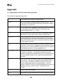
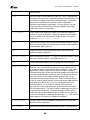
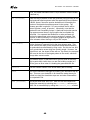
comprehensive list of command line arguments
38
a2
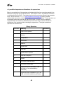
predefined operators and functions for expressions
41
2
NFsim
the network free stochastic simulator
1 overview
NFsim is a generalized biochemical reaction simulator designed to efficiently handle systems
with a very large state space. If this makes sense to you, skip down to the getting started
chapter to try your hand at using NFsim. If you don’t know why you need NFsim, keep reading.
Traditional stochastic or ODE simulation methods require every possible reaction and molecular
species to be explicitly enumerated. For many biochemical systems, this is not a problem.
However, for biochemical systems that exhibit high degrees of combinatorial complexity, as we’ll
explain below, this becomes a major problem indeed. Let’s think about why.
Imagine you have a biochemical reaction system where molecule A can bind to molecule B.
You would then have a simple reaction network consisting of just two reactions:
A + B → A.B
and A.B → A + B
Fine. Now imagine you want to add an additional set of reactions where A can be either
phosphorylated or dephosphorylated. This could be written as:
A → Ap and Ap → A
But wait! You can’t just add the phosphorylation reaction alone! You also have to consider the
phosphorylation reactions when A is bound to B. To consider all the possibilities of the system,
you need to define the following four reactions as well:
Ap + B → Ap.B
A.B → Ap.B
and Ap.B → Ap + B
and Ap.B → A.B
Suddenly, adding two phosphorylation reactions means that you actually have to write down
four additional reactions. If you consider that many signaling systems involve dozens of
interacting molecules in different states, you can see that the complexity of the system becomes
a real problem. That’s why researchers began developing rule-based modeling languages like
the BioNetGen Language (BNGL). Instead of requiring the modeler to specify all reactions,
languages like BNGL only require you to specify reaction rules. For the A and B system
above, with phosphorylation, this would amount to only two reaction rules and could be written
in BNGL as:
A(bSite) + B(aSite) <-> A(bSite!1).B(bSite!1)
A(p~UNPHOS) <-> A(p~PHOS)
In BNGL, we specify molecules by their name and use components of those molecules (as in
‘bSite’, ‘aSite’, and ‘p’) as binding sites that can connect molecules together or as states that
can have a value (as in phosphorylated or not). The details of the language are discussed
elsewhere (http://bionetgen.org), but the idea is simple: the user only has to provide the rules,
and the computer will figure out the rest.
Although the rule-based approach works great for many systems, most simulators (including
standard BioNetGen simulators) still rely on generating all possible reactions from the list of
3
NFsim
the network free stochastic simulator
reaction rules. So, the full reaction network is enumerated. For our A and B example here, this
isn’t a problem because a computer can easily generate and handle 4 extra reactions. For
polymerization, aggregation, or clustering type systems, however, there may be millions, billions
or even an infinite number of possible reactions! In this case, traditional simulators just don’t cut
it. This problem is known generally as combinatorial complexity.
NFsim (aka the Network-Free Stochastic Simulator) works differently than traditional simulation
techniques. It treats each molecule in the system as a separate object that can be connected to
other molecules. Then, by propagating rules directly, the full set of possible reactions (the
reaction network) never has to be enumerated. That’s why we call it Network-Free. NFsim only
keeps track of the state of the system that actually exists, not every possible configuration. This
makes simulating systems with a large reaction network and a high degree of combinatorial
complexity not only possible, but fast as well.
Of course, NFsim shouldn’t be used in every situation. Because molecules are treated as
distinct objects in NFsim, there is an extra computational overhead in storing and maintaining
those objects. The overhead is insignificant when you’re trying to simulate very large systems,
but it does make simulations of simple systems slower than ODEs or other standard stochastic
methods. That’s why we’ve fully integrated NFsim with BioNetGen’s existing capabilities.
BioNetGen already offers efficient simulation of rule-based models using either ODE’s or
Gillespie’s stochastic simulation algorithm. Now, you can write a single model file and choose
exactly how you want to simulate it.
4
NFsim
the network free stochastic simulator
2 getting started
Step 1: download and install NFsim and a free Perl interpreter
NFsim has been tested on a variety of platforms, including Windows (XP, Vista, Windows 7),
Mac (OS X 10.5+ Intel), and Linux. You can download the current version of NFsim from the
NFsim website (http://emonet.biology.yale.edu/nfsim/download/). The full distribution includes a
compatible version of BioNetGen, source code, analysis tools, documentation, and a few
example models.
Once you have downloaded the compressed NFsim file, unzip / untar / install the file to a
directory of your choice. NFsim is a self contained program, so uninstalling NFsim is as easy as
deleting that directory. We recommend that you choose a directory with no spaces in its name
to avoid problems with running the program from the command prompt.
To run BioNetGen, you will need a Perl interpreter. A Perl interpreter usually comes standard in
Linux and Mac operating systems, but not in Windows. If you are running Windows or do not
have a Perl interpreter, you can download ActivePerl, a free interpreter that is available here:
http://www.activestate.com/Products/activeperl/ . Note that you may have to reload your PATH
variable after you install Perl, which you can easily do by logging out then logging back in.
Step 2: open a command line window
NFsim runs from the command line, which gives you more flexibility in running simulations. So
the next step is to open a command line window.
To open a command line window in Windows XP, click on the Start menu, go to Start->run,
and enter ‘cmd’, In Windows Vista and Windows 7, click on the Start menu and enter ‘cmd’
directly into the start menu command bar. In Mac, search for the terminal program, generally
found under Applications->Utilities->terminal. Finally, in Linux, you should already
know how to open the command line, but if not you can usually find it under Applications>System Tools->terminal.
Step 3: test Perl and BioNetGen
With a command line window open, you can now test that your Perl interpreter and BioNetGen
that came with NFsim was installed properly. In the command line window, first test Perl by
typing:
perl -v
You should see the version number of your Perl installation. If you do not, then Perl is not
working or was not installed properly, and you will not be able to run BioNetGen. Please try
reinstalling your Perl interpreter.
5
NFsim
the network free stochastic simulator
Now, make sure BioNetGen is working. First, change directories to location where the
BioNetGen program is located, inside the directory where you installed NFsim, using the cd
command:
cd [install path]/NFsim_vX.XX
where [install_path] is the location where you installed NFsim and X.XX is the version of
NFsim you downloaded. Now, run BioNetGen by entering:
perl BNG2.pl -v
If you see the version of BioNetGen printed, BioNetGen and Perl are working correctly.
Step 4: run NFsim
Now you can run your first NFsim model. If you look in the models directory of the NFsim
installation, you will find a file named simple_system.bngl. This is a BNGL model file that
specifies a simple binding and phosphorylation reaction. You can open the file in any text editor
to see what a BNGL file looks like, and see comments that tell explain the basic parts of the file.
Now try running this model from the command line. While you are still in the BNG directory of
your NFsim installation, enter the command:
perl BNG2.pl models/simple_system.bngl
If NFsim is running properly, you will see messages appear in the command line window that
informs you that the simulation ran. If you encounter an error saying that the NFsim executable
could not be found, and you have an older computer or an operating system that we have not
built a binary for, then you should try to rebuild NFsim for your particular computer architecture
which is relatively simple to do (see Chapter 10: building NFsim locally).
Step 5: visualize your results
After you run the simulation, NFsim will output a file called simple_system_nf.gdat in the
models directory. You can open this file in any text editor you like or load the results into a
program like Matlab (see Chapter 5: getting results). However, with the NFsim installation, we
have also included a simple Java program named PhiBPlot developed to visualize the results
of gdat files. If you have Java installed, you can run PhiBPlot in Windows by double clicking
on the file PhiBPlot.jar in the NFtools/PhiBPlot/ directory, or from the command line
with:
cd [install path]/NFsim_vX.XX
java –jar NFtools/PhiBPlot/PhiBPlot.jar
If the command above does not work, make sure that you have Java installed and visible on
your systems path variable. Then, in PhiBPlot you can choose to load the
simple_system_nf.gdat file and plot the simulation output.
6
NFsim
the network free stochastic simulator
3 working with BioNetGen
NFsim was designed so that models are specified in an extended form of the BioNetGen
Language using .bngl files. The .bngl files can be read and processed by the BioNetGen
program which will create an XML encoded form of your model. This XML format can then be
read into NFsim and simulated. Here we discuss the basic features of a BioNetGen model
specification file. For more advanced BioNetGen features and a complete BioNetGen model
specification file guide as well as graphical tools for creating BNGL files, see the BioNetGen
website: http://bionetgen.org. More advanced NFsim features can be found later in this manual.
Once you have written your BNGL model file, you can simulate the model in a variety of ways
(see Chapter 2: getting started and Chapter 4: running simulations).
a. representation of Molecules and Complexes in BNGL
In BNGL, proteins and other biomolecules are represented as structured objects called
Molecules. Each Molecule may contain any number of Components that represent structural or
functional elements of the protein, such as protein domains and phosphorylation sites.
Components are allowed to have internal states that may, for example, represent a
conformational state or a posttranslational modification of a domain. In BNGL, one can define a
protein S that has a phosphorylation site Y, a binding domain SH2, and a catalytic domain Kin,
as
S(Y~U~P,SH2,Kin~inact~act)
where the Components of S are listed in parentheses together with the possible internal states
of each Component. Internal states are denoted by a list of strings each preceded by ‘~’. Here,
the Y Component may be in either the U state or the P state representing the unphosphorylated
and phosphorylated forms, and the Component Kin may be in either the inact or the act state
representing inactive and active states of the kinase domain. The Component SH2 does not
have any internal states.
Molecules may bind to other Molecules through Components to form complexes. For instance,
a dimeric receptor complex can be defined as
R(DD!1,Y1~U,Y2~U).R(DD!1,Y1~U,Y2~U)
where the two receptors are bound through the link between the dimerization domain (DD) of
each receptor. The ‘.’ is used to group Molecules into a complex. Components linked through
a bond are indicated by an ‘!’ followed by the index number of the bond. Here, a bond with
index 1 links the DD Components of the receptors. Bond indices can be arbitrarily chosen by the
user and are local to the complex in which they are used. Bonds between Components of the
same Molecule are also allowed.
7
NFsim
the network free stochastic simulator
b. structure and syntax of a BNGL file
A BNGL model file for NFsim is comprised of a set of input blocks, each of which begins with
the line begin [blockname] and ends with the line end [blockname]. The set of input
blocks includes: parameters, molecule types, seed species, observables,
functions, and reaction rules.
The parameters block is used to declare numerical parameters that designate initial Molecule
numbers and rate constants. Each parameter is declared on a separate line with the parameter
name followed by the parameter value. Parameters can be either single numeric values or
arbitrary mathematical expressions that reference other parameters already defined. For
example:
begin parameters
FreeReceptorCount
RateFactor
kOn
...
end parameters
500
10
0.3*RateFactor
The molecule types block is used for the declaration of Molecules. This block is optional,
but highly recommended because it allows more comprehensive error checking and reduces the
likelihood of unintended user mistakes in model specification. Each Molecule Type is declared
on a separate line. For example, an input block that defines a receptor, R, and signaling protein,
S, might look like
begin molecule types
R(DD,Y~U~P)
S(Y~U~P,SH2,Kin~inact~act)
end molecule types
The seed species block is used for the declaration of the molecular species that are initially
present in the system. Note that any Component that has an associated state variable must be
in a defined state. Each species is declared on a separate line followed by its initial count,
which may be a defined parameter or arbitrary mathematical formula. Note that in NFsim,
molecules are treated as separate objects, so decimal values in the number of species are not
supported. Parameters that are used to define initial species counts will be rounded down to
the nearest whole integer value. For example, we can define three initial molecular species, a
free receptor, a receptor dimer, and a free signaling protein as
begin seed species
R(DD,Y1~U,Y2~U)
FreeReceptorCount
R(DD!1,Y1~U,Y2~U).R(DD!1,Y1~U,Y2~U)
250
S(Y~P,SH2,Kin~inact)
1000
end seed species
8
NFsim
the network free stochastic simulator
The observables block is used for declaring variables that count the number of Molecules in a
system that match a pattern. Observables are useful for defining the output of a model and
introducing rate laws defined as mathematical expressions of the time-dependent state of the
system. An example of an Observable definition is
begin observables
Molecules
PhosRec
...
end observables
R(Y1~P)
which gives the total number of Receptors that are phosphorylated at the Y1 Component at any
time during the simulation. The Molecules keyword indicates that the Observable will count a
Molecule every time it matches the pattern. BNGL also allows users to define Species
Observables that count the number of complexes that have at least one Molecule matching the
pattern. For instance, a Species Observable will count a dimer of two phosphorylated
receptors only once.
The functions block is used for defining mathematical expressions that reference defined
parameters and Observables of the system. The functions block is a new feature of BNGL
that was introduced to support functions in NFsim. Therefore, if the functions block is used
in a model, it can only be simulated with NFsim. Below we demonstrate the declaration of a
simple function named ActivationFunc that references the Observable pattern named
PhosRec defined earlier, and constant parameters n and Kd that can be defined in the
parameters block.
begin functions
ActivationFunc()= (PhosRec^n) / (Kd^n + PhosRec^n)
...
end functions
Once declared, functions can be used as the rate law for reaction rules. In this case,
ActivationFunc is a global function because it counts the total number of phosphorylated
receptors in the system. NFsim also supports local functions which are evaluated separately for
each molecular complex and require a slightly different syntax. For a complete description of
the definition and usage of global and local functions, see Chapter 6: functionally defined
rate laws.
Finally, at the heart of BNGL is the reaction rules block used to define the reaction events
that can occur in the system. Each Rule is declared on a separate line. The two basic types of
transformation operations that are typically defined in Rules are: (1) change Molecule
connectivity by making or breaking a bond and (2) change the internal state of Components.
Other operations, such as Molecule synthesis, degredation, and incrementing the numerical
internal state value of a Component are not discussed here. Below is an example reaction
rules block that defines a dimerization rule with a binding operation and phosphorylation rule
with an internal state change operation.
begin reaction rules
R(DD) + R(DD) -> R(DD!1).R(DD!1) kOnDimer
R(DD!+,Y1~U) -> R(DD!+,Y1~P) kPhos
9
NFsim
the network free stochastic simulator
...
end reaction rules
These Rules illustrate a number of important elements of BNGL syntax. The first Rule states
that two receptors with unbound DD Components (underlined) can dimerize by forming a bond
between the DD Components with second order kinetic rate kOnDimer. Notice that the Y1 and
Y2 Components are not defined in the rule. When Components are not defined, they do not
affect the rate of the rule. In other words, this rule applies to all receptors with unbound DD
Components regardless of the internal or binding state of Y1 and Y2. The power of BNGL lies in
this aspect of Rules: only the minimal conditions for the event to occur need to be explicitly
defined, thus eliminating the need for the user to enumerate every possible combination.
The second Rule defines the phosphorylation of Y1 Component (underlined) by changing the
internal state of Y1 from U to P with first order kinetic rate kPhos. In this Rule there is the added
constraint that the DD Component must be bound for the reaction to occur indicated by the ‘!+’
following the DD Component. Notice again the omission of the Y2 Component of R, which
means that the Rule is applied regardless of the state of the Y2 Component.
In any particular Rule, multiple internal state changes or binding and unbinding operations can
be applied to arbitrarily large molecular complexes. Although the rules shown here are
irreversible, BNGL also permits the definition of reversible reactions by defining a Rule with the
double headed arrow, ‘<->’, and providing a second rate constant or functional rate law.
10
NFsim
the network free stochastic simulator
4 running simulations
a. running from BioNetGen
The easiest way to run an NFsim simulation is to directly invoke NFsim through BioNetGen.
Just place the following command at the end of your BNGL model specification file:
simulate_nf{suffix=>nf,t_end=>[sim_length],n_steps=>[output_steps]};
Then, run BioNetGen with the BNGL file from the command line as you normally would (see
Chapter 2: getting started). The suffix parameter tells BioNetGen how to name the output file.
The simulation length and output steps tell NFsim how long and when to output the observables
of the system. So if you wanted to run your simulation for 100 seconds, and output 50 times (or
once every two seconds), you would enter:
simulate_nf{suffix=>nf,t_end=>100,n_steps=>50};
At each output step, the counts of every Observable will be written to a .gdat file (see Chapter
5: getting results). When you run NFsim in this way, BioNetGen automatically generates the
XML file needed by NFsim for you, and searches in the [install_path]/bng/bin directory
for the correct NFsim executable.
If you are familiar with BioNetGen already, then you will recognize that this is similar syntax to
running a stochastic or ODE simulation in BioNetGen. Note, however, that NFsim does not
store all model details after a simulation. Therefore, NFsim ignores the BioNetGen action
keywords such as setConcentration, saveConcentrations, and
resetConcentrations.
NFsim also accepts a number of command line arguments to fine tune your simulation that are
listed in Appendix a1 and described through this user manual. You can pass any of these
extra parameters to NFsim from BioNetGen by setting the param argument in the simulate_nf
command. For instance, if you wanted to turn on verbose output (with the NFsim command line
argument –v) as well as setting the universal traversal limit to be 3 (NFsim argument –utl),
you can write:
simulate_nf({suffix=>nf,t_end=>100,n_steps=>50,param=> “-v –utl 3”});
b. running from a BNG XML file
You don’t need to always invoke NFsim from BioNetGen. Instead, you can run NFsim directly
using an XML file that was generated by BioNetGen. This allows you to call NFsim directly from
a shell script, for instance, without having to run BioNetGen. Often this provides more flexibility
and efficiency when you have to run multiple simulations. First, you do have to run BioNetGen
11
NFsim
the network free stochastic simulator
once in order to generate an XML file that NFsim can read. To do so, add the following
command to the end of your BNGL file:
writeXML();
This command will produce an XML encoding of your model. Just run the BNGL file as you
normally would using BioNetGen (see Chapter 3: working with BioNetGen). You can also call
BioNetGen with the –xml flag as:
perl Perl/BNG2.pl –xml [BNGL_file_name]
Assuming you are in the NFsim installation directory. This command will also create an xml file.
Once you have an XML file, you can run NFsim directly from the command prompt. To do this,
again from the base installation directory, run the command:
bin/NFsim_[version] –xml [BNG_XML_file_name]
where [version] is the executable version of NFsim that is specific to your operating system.
You can look in the bng/bin directory for the set of NFsim executables, and select the one that
matches your computer. Note that if you are running NFsim from windows, you must be sure to
add the .exe file extension when you run NFsim.
When you run NFsim from the command line directly, you must pass in additional parameters to
tell NFsim how long to simulate and how often to generate output. There is a complete list of
parameters in Appendix a1, but for easy reference, here are the basic parameters that you will
most often use.
-xml
used to specify the input xml file to read. the xml
file must be given directly after this flag.
-o
used to specify the output file name, which is given
directly after this flag.
-sim
used to specify the length (in seconds) of a
simulation when running an xml file. Fractional
seconds are valid. For instance, you could use: -sim
525.50
-oSteps
used to specify the number of times throughout the
simulation that observables will be outputted. Must
be an integer value. Default is to output once per
simulation second.
12
NFsim
the network free stochastic simulator
c. running from Matlab using the runBNG function
With NFsim, we have also provided a Matlab function that can run BioNetGen directly from
Matlab using the included function "runbng", which is available in the NFtools directory. To
run BioNetGen in Matlab, open Matlab and change the current Matlab directory to the root
directory of your NFsim installation. Once you are in the correct directory, add the NFsim tools
directory to your Matlab path so that you can call the runbng function by entering:
addpath(‘NFtools/’);
Then, you can run BioNetGen, and NFsim if it is called from the model file, as:
[data,varNames,consoleOutput,figureHandles] = . . .
runbng('pathToDirectory','bngl_file_name');
This will run BioNetGen on the given BNGL file located at the specified path. For instance, to
run BioNetGen on the example model 'simple_system.bngl' in the 'models' directory, you would
enter:
runbng('models','simple_system.bngl');
The first time you run this function, you will have to provide the installation path of NFsim so that
the function can identify the necessary executable files. Then, this function will run the model
specified and plot any results that are generated in GDAT files. If there is only one GDAT
output file created, it will return the data and variable names from that file as 'data' and
'varNames'. If there are multiple GDAT files, 'data' and 'varNames' will be cell arrays where
each cell contains the output of a given GDAT file. (note: you can use the iscell function in
Matlab to determine if the returned variable is a cell array or not).
The function also returns the ‘consoleOutput’ of the run (which includes basic information
about what BioNetGen and the simulation are doing) and ‘figureHandles’ which stores an
array of handles to all the figures generated so you can change them and set any figure
properties you need.
d. running from an RNF script
NFsim can run from an RNF (Run NF) script that is easy to learn, but powerful because you can
change parameters mid-simulation. It is one of the more advanced ways to run NFsim, but is
ideal for large projects that require multiple revisions and runs.
There is an example RNF script in the models directory of your installation named
example.rnf. This is the best place to learn about the structure and commands of an RNF
script, and documentation on the RNF format can be found in that script file.
13
NFsim
the network free stochastic simulator
To run an RNF script, first create an RNF file according the specifications in example.rnf. Then
use the NFsim argument when running the file. For instance, to run an RNF file from within
BioNetGen
bin/NFsim_[version] –rnf [RNF_file_name]
use the NFsim argument when running the file. For instance, to run the example.rnf file,
change directories to the models directory, and run NFsim as:
../bin/NFsim_[version] –rnf example.rnf
In Windows, make sure you add the .exe file extension, and use backslashes instead of forward
slashes. Even though Windows will often interpret forward slashes correctly, when searching
for an executable file, it requires backslashes. Therefore, you will have to run the file in
Windows as:
..\bin\NFsim_[version] –rnf example.rnf
Note that when you run an RNF file that specifies an XML model (as in example.rnf), the
path to the XML file is interpreted as relative to your current path, not the location of the RNF
file. Thus, if you run example.rnf from the main NFsim installation directory instead of from
the models directory, NFsim will be unable to find the XML file simple_system.xml.
14
NFsim
the network free stochastic simulator
5 getting results
A simulation is only as good as the results it can output. NFsim provides two main options for
extracting results which are both described below.
a. basic Observables and output
Observables are the typical method of getting output from an NFsim simulation. All you have to
do is define the set of Observables you want to watch during the simulation in the BNGL model
file, and run that file with BioNetGen and NFsim. NFsim will automatically generate an output
file with the name [model_name]_nf.gdat. GDAT files are simple ASCII text files where the
count of each Observable at every output step is given in a simple table format. These text files
can be opened in any standard text editor. To set the number of times that NFsim produces
output during a simulation, use the –oSteps command line flag or set it in the
simulate_nf(…) call in BioNetGen (see Chapter 4: running simulations).
GDAT files can be easily opened and graphed in any other program, from Matlab and
Mathematica to Excel. In Matlab, the easiest way to read in the results is by using the function
tblread. Simply call it in Matlab as:
[data,headerNames] = tblread(‘[model_name]_nf.gdat’);
And the results will be available in a two-dimensional matrix named data.
In some cases, you will have a lot of information to write to a file. When you are running
simulations with many Observables with many output steps or if you have to thousands of
output files to generate, you will find that reading an ASCII text file can take time. Additionally,
ASCII text files take up a lot of room on your hard disk. NFsim offers a way to get around this
by outputting the results in a binary format. To output your results to a binary file instead of an
ASCII GDAT file, use the NFsim command line parameter –b.
The binary file will be saved with the same name as the GDAT file, except with the extension
.dat. The binary file is saved as a long list of numbers that are should be 8 bytes long. When
outputting to binary format, NFsim will also generate a header text file that provides you with the
header names of each column.
You can write your own program to read the binary file, or you can use the provided
readNFsimBinary.m function in the NFtools directory. To run the function, change the
current directory in Matlab to the installation directory of NFsim. Once you are in the correct
directory, add the NFsim tools directory to your Matlab path so that you can call the function by
entering:
addpath(‘NFtools/’);
Then you can call the function as:
15
NFsim
the network free stochastic simulator
[data,varNames] = readNFsimBinary([binary_file_name]);
This function will return the data and header names in the same style as tblread.
b. dump System state
Sometimes the default set of observables is not enough to get the results you need. This is
especially true of the types of systems that NFsim is very good at simulating. For instance, if
you want to simulate receptor aggregation, you would probably like to know what the average
aggregate size is. However, you can’t easily write a BNGL observable to capture this.
To solve this problem, we built functionality to dump the complete state of the system at
particular time steps in a binary format so that any observable, no matter how complex, can be
calculated and analyzed after the simulation has run. You can tell NFsim to dump the state of
the system using the –dump flag. The dump flag is designed so that you can tell it when and
where to dump the output. Call the dump flag as:
–dump “[1:1:10;25;50]->dumpDir/”
The string given to the dump flag tells NFsim the times to output the complete state of the
system and the directory to place all the files that are generated. You can specify and directory
for this use, but be careful because there will be a lot of files. You can specify the output times
in a Matlab style format where the times are delimited by semicolons, and output times can be
arrays in the form start:step:end. For instance, in the above example, the state of the
system will be dumped at times 1,2,3,4,5,6,7,8,9,10,25, and 50.
Then, you can write your own program to process the file or use our included set of Matlab
scripts to read the data into Matlab. The Matlab scripts also include some basic functionality to
look at average aggregate sizes or the average value of local functions evaluated on different
complexes throughout the system. The set of Matlab scripts, along with additional
documentation on their usage, can be found in the NFtools/NFanalyzeDump directory.
16
NFsim
the network free stochastic simulator
6 functionally defined rate laws
NFsim permits the definition of both local and global Functions allowing you to build
approximations, cooperativity, non-linear reaction rates, and conditional rules into your model.
This feature has also been added to the BioNetGen Language so that functions are easy to
define and use in rules. Here we discuss the definition and usage of global functions that
depend on the state of the entire system. The next chapter on distribution of rates reactions
(or DOR reactions) will discuss how to use local Functions to influence reaction rates according
to local context.
Note that although functions can be used to define the Michaelis-Menten approximation, like in
BNG, NFsim supports the MM keyword to quickly define the quasi-steady-state MichaelisMenten approximation in rate laws. The usage of the MM function is identical to that of BNG.
Namely, use the function in place of a rate as: MM(kcat,Km), where kcat and Km are the
corresponding parameters of the Michaelis-Menten approximation. Note that NFsim does not
support the SAT keyword that is available in BNG. In all cases, as it is more accurate, use the
MM keyword instead.
a. defining global functions in BNGL
Global Functions are defined in terms of constant parameters or Observables of the system.
The typical Observables in a model, which are used for output, can be thought of as global
Observables because they are computed over every molecule or complex throughout the entire
system. Because functional definitions depend on Observables, the Observables block must be
declared in the BNGL file before the functions block.
The syntax for defining global functions is as follows:
begin parameters
k1 20
k2 0.5
end parameters
begin observables
Molecules Ap A(p~phos)
Molecules Btot B()
end observables
begin functions
testFunc() = k2*(Ap+Btot)/k1
end functions
Notice how we define testFunc() as a mathematical expression of the Observables and
parameters in the system. Global functions cannot take any arguments. Arguments to
functions are reserved for local functions that are described in chapter 7. NFsim does not
currently allow functions to be defined in terms of other functions, although when declaring a
17
NFsim
the network free stochastic simulator
rule, the rule can include an expression referencing multiple functions. Furthermore, functions
cannot explicitly reference the current simulation time.
A number of mathematical operators and predefined functions can be used in expressions, and
include the standard operations you might expect. For a complete listing, see Appendix a2.
b. using global functions in rate laws
Once global functions are defined, they can be used to influence the rate of any rule in the
system. For instance, we can define a state change of A that occurs with the rate given by the
testFunc() function.
begin reaction rules
A(m~0) -> A(m~2) testFunc()
end reaction rules
We can also use additional mathematical expressions to control the rate when the rule is
declared. For example, the following is valid BNGL and will be processed as expected:
begin reaction rules
A(m~0) -> A(m~2) (k1*testFunc())+testFunc()^2
end reaction rules
An important aspect of functional rate laws to keep in mind is that, like normal rate constants,
the combinatorial terms are automatically factored into the propensity of the rule. In other
words, rate terms and functions are defined in terms of the macroscopic, per site rate, as
opposed to the total macroscopic propensity. To illustrate, consider the following model:
begin functions
testFunc2() = 50
end functions
begin reaction rules
A(m~0) -> A(m~2) testFunc2()
end reaction rules
In this model, the combinatorial term of reactant A is factored in for you, so that the total
propensity of the rule is = 50*|A(m~0)|, where |A(m~0)| is the number of molecules that
match the pattern A(m~0). The model above will have the same behavior as this model:
begin reaction rules
A(m~0) -> A(m~2) 50
end reaction rules
However, the automatic inclusion of the combinatorial term is not always desirable. In some
cases, for instance with the Michaelis-Menton approximation, the propensity of the rule may
18
NFsim
the network free stochastic simulator
depend on a higher order term of the reactant numbers. To provide maximal flexibility in these
cases, the TotalRate keyword is available that allows you to take FULL control of the
macroscopic propensity term. To use this keyword, simply define your rule as:
begin functions
testFunc2() = 50
end functions
begin reaction rules
A(m~0) -> A(m~2) testFunc2()
end reaction rules
TotalRate
By activating this keyword, the total propensity will be defined completely by the expression you
give. Therefore, the propensity of the rule defined above will be simply 50, regardless of the
number of reactants there that exist in the system. When using this syntax, be careful because
it is easy to write a model that is not biochemically correct.
When using the TotalRate keyword, it is often necessary to refer to the number of reactants in
the system and use that number in an expression. One way to do this is to define an
Observable that tracks the reactant. This approach, however, is prone to error because you can
change the reactant pattern without changing the Observable pattern. NFsim provides a better
and computationally more effecient method to handle these situations. NFsim has a built in
function called reactant_N() where N can be either 1 or 2 depending on the reactant you are
referencing. This function returns the number of reactants that match either the first or second
reactant pattern. This syntax is currently not part of standard BNGL syntax, so to use this built
in function, you have to declare the reactant_N() functions in the functions block. For
example, this is how you would declare a propensity that is defined in terms of the squared
number of reactants:
begin functions
testFunc2() = 50
reactant_1()
end functions
begin reaction rules
A(m~0) -> A(m~2) (reactant_1()^2)*testFunc2()
end reaction rules
TotalRate
To give another example for the bi-molecular reaction case:
begin functions
testFunc2() = 50
reactant_1()
reactant_2()
end functions
begin reaction rules
A(m)+B(a) -> A(m!1).B(a!1)
(reactant_1()^2)*reactant_2()*testFunc2() TotalRate
end reaction rules
19
NFsim
the network free stochastic simulator
c. outputting the value of global functions
The value of global functions can always be recalculated at any of the output steps by using the
values of the Observables at that step and reevaluating the same function yourself. But to
make things easier, and to make sure NFsim is doing what it’s told, there is a command line flag
that tells NFsim to output the value of each global function at every step into the default .gdat
output file. When calling NFsim, just call it as:
./NFsim_[version] […other parameters…] –ogf
where ogf stands for “Output Global Functions”. Then take a look at your .gdat file. This is
useful for making sure NFsim is evaluating exactly how you think it should.
c. using conditional expressions in functions
A very useful feature of all functions is that they can include conditional expressions. Here is a
brief overview of how to add conditional expressions into your functions and some of the typical
reasons for doing so.
Conditional expressions allow the function to be evaluated completely differently based on some
condition. The way to add this ability is to use an if statement in your function. The best way
is to start with an example, so here you go:
begin observables
Molecules TimerCount Timer(t~ON)
end observables
begin functions
testFunc3() = if(TimerCount>1000,50,0)
reactant_1()
end functions
begin reaction rules
Timer(t~OFF) -> Timer(t~ON) 1
A(m~0) -> A(m~2) reactant_1()*testFunc3()
end reaction rules
In the above example, we define an Observable that counts the number of Timer molecules in
the ON configuration. We then define a function that checks if the TimerCount Observable
exceeds 1000. If the TimerCount Observable is greater than 1000, then the function
evaluates to 50. Otherwise, the function evaluates to 0. This way, we can selectively turn on a
reaction (say where A changes its m state) only when the Timer molecule observable exceeds
1000. The expressions inside the if statement can be as complicated as you want. You can
20
NFsim
the network free stochastic simulator
even nest if statements inside of each other to get arbitrarily complex logic in your rules.
Finally, keep in mind that BNGL now supports logical and / or expressions, as && and ||
respectively, to detect complex conditions. For example, the following is valid:
testFunc3() = if(TimerCount>1000||TimerCount<100,50,0)
And will set the function to 50 if the TimerCount is either above 1000 or less than 100.
Conditional expressions can be useful in a variety of contexts. One situation where it proves to
be useful is if we ever want to conserve the bulk concentration of some molecule in solution, but
we don’t want to model the entire cell, say. We can do this by selectively turning on a molecule
generation function whenever the number of that molecule in solution drops below the
concentration. Another useful case is if we want to turn on a set of reactions only after some
conditions are met. For instance, if we don’t want to simulate the cell division reactions until we
have grown to a certain size, or if we don’t want to turn on metabolic reactions until a particular
sugar to be metabolized is produced.
21
NFsim
the network free stochastic simulator
7 distribution of rates reactions
Global functions with conditional expressions are very powerful, but are still not enough to
adequately describe behavior like cooperativity. The problem arises out of combinatorial
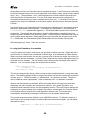
complexity. In current BNGL and other rule-based modeling languages, for every possible rate
of a reaction or chemical transformation, a separate rule must be written. For instance, if
molecule A can be phosphorylated at 3 sites, and each possible phosphorylation state causes A
to bind B with a distinct rate, then you would normally have to write out all combinations of A:
A(p~0,b)
A(p~1,b)
A(p~2,b)
A(p~3,b)
+
+
+
+
B(a)
B(a)
B(a)
B(a)
->
->
->
->
A(p~0,b!1).B(a!1)
A(p~1,b!1).B(a!1)
A(p~2,b!1).B(a!1)
A(p~3,b!1).B(a!1)
rate0
rate1
rate2
rate3
Of course this is time consuming and prone to error if there are many more states that A can
exist in. Sometimes, enumerating all the states is not even possible, for instance, if you have a
polymer forming and the elongation depends on the length of the polymer. Then, for every
single length polymer that can form, you need to write a slightly different rule with a different
rate. This gets you back to the problem that NFsim was designed to solve.
However, in most cases, you can simply write a function that describes very well how the rate
changes according to some property, say the length of the polymer or the phosphorylation state
of the molecule. That function might be as simple as: rate of elongation = length of polymer * k.
This is a function that cannot refer to just global Observables, the way global functions are
defined, because the length of the polymer is not a global Observable! It is different for every
single polymer you are simulating. However, NFsim and BNGL provide a framework for
describing such systems in a straightforward way. We call this syntax local Functions because
these functions reference variables that are local to individual molecules or molecule
aggregates. Reactions that call local functions are referred to as Distribution of Rates
Reactions because reaction will have a distribution of rates depending on the value of the local
variables.
a. defining local functions in BNGL
Local functions can be defined as follows:
begin observables
Molecules Ap A(p~phos)
Molecules Am0 A(m~0)
Molecules Btot B()
end observables
begin function
localTestFunc(x) = (Ap(x)+Btot)/20
localTestFunc2(x,y) = Am0(x)*(Ap(y)+Btot)/20
end function
22
NFsim
the network free stochastic simulator
Observables used by local Functions can be declared as before. Local Functions are identified
by the fact that they accept one or more arguments of an arbitrary name, which we have named
here x and y. The arguments x and y that are passed into functions defines the scope over
which the function is evaluated over. For now, think about the scope as a small group of
connected molecules that you want to evaluate the function over. If a function is not given an
argument, the scope is considered to be the entire system, and the function becomes a global
Function.
In a local Function, any Observable that is required to be evaluated over a local scope must be
passed the appropriate scope argument. For example, the Observable Ap as referenced in
localTestFunc(x) is passed the argument x. Such Observables are said to be local to the
scope given. That means that the number of times the Observable is matched in the local
scope is counted, instead of over the entire system. Unlike functions, Observables can only be
given a single scope argument. Observables that are not provided with a scope, such as the
Btot Observable, are evaluated like global Observables over the entirety of the system.
Still following along? Good. Then let’s move on.
b. using local functions in a reaction
Local Functions only become useful once you use them to define a rate law. Rules that use a
local Function in a rate law are considered, in NFsim lingo, as a Distribution of Rates reaction.
When you use a local function in a rate law, you now have to declare the scope over which you
want the local function evaluated. Currently, NFsim supports two scopes, although this may be
extended in future releases. The first scope involves all molecules connected to the marked
Molecule. You can use this scope in a local function as follows:
begin reaction rules
%c::A(m~0) -> %c::A(m~2) localTestFunc(c)
end reaction rules
This rule is interpreted just like any other, except we have marked molecule A using the syntax
above. This marking signals NFsim to compute the scope over the set of molecules connected
in some way to A. The percent label (%) indicates that c is a pointer to a scope. The name c
can be whatever name is appropriate. Here we arbitrarily use c to represent a complex.
When a rule like the above is declared, NFsim will create the local Function and evaluate it
separately over each complex that contains an A reactant. As in global Functions, your
expression takes complete control over the propensity function. The local Function assigns the
propensity for a given reactant set to undergo the reaction; consequently, the Function should
not include terms that compute the overall population reaction rate. The overall rate is
automatically calculated by summing the local rates over all possible reactant sets.
The second scope that can be defined is over a SINGLE molecule. To define the scope of a
local function over a single molecule, instead of the entire connected complex, you can define
the reaction rule as:
A%mol(m~0) -> A%mol(m~2) localTestFunc(mol)
23
NFsim
the network free stochastic simulator
In this case, the local function will be evaluated over the single molecule A, and ignore
everything that A is connected to. This functionality is useful in certain situations.
When using local Functions in your models, there are a couple important items to keep in mind.
First, local Functions do make NFsim run slower as the local Function must be evaluated over
each connected complex and explicitly remembered. Second, the scope of local Functions can
only be defined over a single reactant per rule (for an exception, see 7.c). Even though local
Functions can accept multiple scopes, the scopes must all be found in a SINGLE reactant. This
is because it is practically impossible to efficiently simulate a rule that depends functionally on
both reactants in a local way. To do so would require computing the local Function over each
pair of reactants. For just 100 molecules in each reactant of a bi-molecular rule, this amounts to
calculating the function for 10,000 pairs. Therefore, we don’t allow it and the following rule will
not work, at least in the way that you would like it to:
%c1::A(b) + %c2::B(a) -> %c1::A(b!1).%c2::B(a!1) localTestFunc2(c1,c2)
However, to reiterate, you can indeed define a function that has multiple scopes, as in:
%c::A%mol(m~0) -> %c::A%mol(m~2) localTestFunc(c,mol)
This would evaluate the first scope, c, as the set of molecules connected to A, and the second
scope, mol, as the molecule A only.
c. local functions defined over two reactants
In the general case, the scope of a local Function is restricted to a single reactant. But there is
one special case implemented that bypasses this restriction (v1.11+). A local function may be
defined over two reactants if the rate function can be factored into a product where each term
depends on only one reactant, i.e. 𝑓 𝑥, 𝑦 = 𝑔 𝑥 ⋅ ℎ(𝑦). This special type of local function is
accessed with the special rate law FunctionProduct(“g(x)”,“h(y)”).
Let’s illustrate a function product with an example. Consider an aggregation model with two
molecule types, A and B. When an aggregate grows larger than five A molecules, the aggregate
will become immobile. We want to exclude immobile aggregates from further aggregation, so
our binding rule must assign a zero rate to any pair that includes an immobilized aggregate. We
can accomplish this using the FunctionProduct rate law:
begin molecule types
A(b,b,b)
B(a,a)
end molecule types
begin observables
# count A molecules in aggregate
molecules Atot A()
end observables
24
NFsim
the network free stochastic simulator
begin functions
# return 1 if u is mobile, 0 otherwise
mob(u) = if( Atot>5, 0, 1 )
end functions
begin reaction rules
# bind A and B, only if both are mobile
%x:A(b) + %y:B(a) FunctionProduct(“kp*mob(x)”,“mob(y)”)
end reaction rules
There is a possibility that a future release of NFsim will extend local functions to sums over
functions of single reactants, i.e. 𝑓(𝑥, 𝑦) = 𝑔(𝑥) + ℎ(𝑦).
25
NFsim
the network free stochastic simulator
8 fine tuning your simulations
NFsim provides you with a number of advanced options for running and optimizing your
simulations and extracting exactly the output that you need. Often your simulation can be sped
up by employing one of the performance tweaks mentioned below. There are also some more
tricky syntactical features of BioNetGen that have special relevance to how simulations are run.
These are also discussed in this chapter.
a. on-the-fly Observables
By default, observables are calculated on-the-fly. This means that at each simulation step, all
Observables in the system are updated. This calculation of Observables is essential for
accurately updating the rates of reactions that depend on those Observables. See the chapter
on functionally defined rate laws. Therefore, if you use functionally defined rate laws,
Observables will always be calculated on the fly. In general, however, this calculation is not
necessary. You do not need the value of Observables at every simulation step; you only need
Observables when you actually output the Observables!
NFsim provides the option to recalculate the Observables only when you need them. This is
useful when the number of simulation steps between each output step is greater than the
number of molecules in the system. This may or may not be true for your simulation, so you
should try turning on or off this option to see which is more efficient. To turn off on the fly
computations of observables, call NFsim as:
./NFsim […other parameters…] –notf
where notf stands “Not On-The-Fly”.
b. universal traversal limits
Although it is activated by default to an acceptable value, you can often speed your simulations
significantly by using this tweak. In NFsim, each molecule is treated as a separate software
object. When a reaction is fired, a particular molecule may bind another, unbind, or change its
state. When a molecule is updated, all molecules it is connected to may also need to get
updated. By default, NFsim will update as many molecules as necessary based on the size of
the largest reactant pattern in the rule-set. Sometimes however, based on the structure of the
reactant patterns, this is not necessary. Only the nearest neighbors to the reaction center
(molecule which is being updated) in a large aggregate need to be updated.
With the universal traversal limit, you can set the distance neighboring molecules have to be to
the site of the reaction. To set the universal traversal limit, call NFsim as:
./NFsim […other parameters…] –utl [integer]
where the integer is the limit you want to set. When NFsim then searches for neighboring
molecules that might have to be updated, it will only search to that depth.
26
NFsim
the network free stochastic simulator
The lower you set the universal traversal limit, the less molecules will be checked and the faster
your simulation will go. However, be careful as NFsim does not double check your limit. If you
set the limit too low, and not all molecules are correctly being updated, then you will either run
into a simulation error or your results will be incorrect. Setting the limit to the number of
molecules in your largest reactant pattern is usually high enough. Another way to double check
is to run simulations with a traversal limit and without to see if you are missing any updates.
By default, the traversal limit is set to the size of the largest reactant pattern, which is
guaranteed to produce correct results because NFsim will always find the changes that apply to
every reactant pattern in the system. In many cases, this provides enough speedup and you
will not have to worry about directly setting the traversal limit. In other cases, however you may
have a very large pattern, but the maximal number of bonds you need to traverse to make sure
that pattern can always be matched is low. This will happen, for instance, when many
molecules are connected to a single hub molecule. In these cases, setting the traversal limit
yourself can produce significant speedups.
c. aggregate bookkeeping
NFsim by default tracks individual molecule agents, not complete molecular complexes. This is
useful and makes simulations very fast, but is not always appropriate. For example, in some
systems it is necessary to block intra-molecular bonds from occurring to prevent unwanted ring
formation. However, to check for intra-molecular bonding events, complete molecular
complexes must be traversed. NFsim, however, provides an aggregate bookkeeping system for
molecular complexes that form by assigning each connected aggregate a unique id. Then, it
becomes easy to check if any two molecules are connected. The trade-off is that there is an
overhead involved with maintaining the bookkeeping system with a cost that depends on the
size of the molecular complexes that can form.
The standard behavior of BioNetGen is to assume complex bookkeeping so that intra-molecular
bonds are kept separate from inter-molecular bonds. For instance, in a reaction rule like:
A(b) + B(a) -> A(b!1).B(a!1)
kOn
BioNetGen will only allow binding reactions between a molecule ‘A’ and molecule ‘B’ if ‘A’ and
‘B’ are on separate complexes. In NFsim, however, this is not enforced and any ‘A’ molecule
would be able to bind any ‘B’ molecule regardless of which complex they are on. In many
cases, this is ok and is the desired behavior. In other cases, you might want to use
BioNetGen’s default behavior, in which case you will have to turn on aggregate bookkeeping.
Aggregate bookkeeping is also necessary for computing Species Observables, which are
Observables evaluated only once per connected complex. This is useful when you want to
query your system for the number of complexes that contain at least one type of molecule or
other pattern. For more information on Species Observables, consult the documentation from
the BioNetGen website.
To turn on aggregate bookkeeping, simply run NFsim as:
27
NFsim
the network free stochastic simulator
./NFsim […other parameters…] –cb
where ‘cb’ stands for complex bookkeeping.
d. restricting the number of molecule agents
In many biochemical systems, Molecules are dynamically created and destroyed. In NFsim,
whenever a Molecule is created or destroyed, a new agent must be added or removed from the
simulation. Each molecule agent must remember its current state, so requires a small amount
of memory. Therefore there is an inherent limit, based on your machine, on the number of
molecules you can create in memory. Depending on your operating system, when this limit is
reached your computer will start using the hard-disk to store memory making your computer run
incredibly slow occasionally to the point of freezing. To prevent your computer from running out
of memory in case you accidentally create too many molecules, NFsim sets a default limit of
100,000 molecules of any particular Molecule Type from being created. If the limit is exceeded,
NFsim just stops running gracefully, thereby potentially saving your computer.
In some cases, however, you may in fact want more than 200,000 molecules of a given type
and you may have more than enough memory to store several million agents. In that case, you
can change the agent limit restriction by running NFsim as:
./NFsim […other parameters…] –gml [limit]
where the flag gml stands for the global molecule limit (per MoleculeType). You might even
want to set the limit lower than 200,000 so that you can make sure you are not generating many
more molecules than you expect.
e. connected-to syntax
The BioNetGen Language allows you to declare that two molecules are connected, without
explicitly giving the bond path between those molecules. For instance, you can define a pattern
as:
A().B()
to match all times where A and B are connected by some path. This syntax is powerful as it
allows you to overcome the combinatorial complexity of having to specify every single
combination of bonds where A is connected to B. Some systems require this syntax to be
specified correctly. However, the connected-to syntax is also incredibly dangerous. Consider
the actual molecule complex instance here:
B(a,a!1).A(b!1,b!2).B(a!2,a!3).A(b!3,b)
In this case, the pattern A().B() will be able to map onto this complex four times, once for
every time you can find a unique A and B in the complex. Therefore, when you have patterns
that use the connected-to syntax, NFsim will have to look for all combinations that match. This
28
NFsim
the network free stochastic simulator
can make your simulation run very slow depending on the pattern and the molecular complexes
that form in your system. So if you are just using this syntax as a shortcut because you don’t
want to write out the bonds, don’t! If you are using it because you genuinely cannot express all
the combinations that the two molecules might be connected, then by all means, go ahead.
While on the subject of the connected-to syntax, there are a few caveats worth mentioning in
the way rules are interpreted. First, consider the following reaction rule:
A(p~U).B() -> A(p~P).B()
kPhos
In such a rule, the only molecule that is being transformed is A. The molecule B is only
providing context for the rule. In other words, the rule can be read as “A can be phosphorylated
when it is in some complex with B with rate kPhos”. Therefore, it doesn’t matter how many B’s
are connected to A, so long as we have one. Thus, a complex that looks like this:
A(p~U,b!1,b!2).B(a!1).B(b!2)
as expected, A will be phosphorylated with rate kPhos, even though there are two places where
B can match. These type of “context” checks are actually performed relatively quickly be
NFsim. NFsim simply searches, in the same way that molecules are traversed during updates,
for the first B molecule it can find. Once it finds one, the B molecule gets mapped and the
search is over. Even in very large aggregates, if the B molecule is nearby, the search will be
over quickly.
On the other hand, consider the following rule:
A(p~U).B(p~U) -> A(p~P).B(p~P)
kPhos
In this case, both A and B molecules are updated by the rule, and A and B are on separate sides
of the operator, essentially in disjoint sets. The rule is interpreted as “every pair A and B
occurring in a complex where both are unphosphorylated, they can both be phosphorylated with
rate kPhos”. This case is trickier for NFsim to handle because instead of searching until a
single B is found, all matching A().B() pairs must be returned. NFsim will do this, if you ask,
but it will affect the rate of the reaction in perhaps a surprising way. Consider the complex:
A(p~U,b!1,b!2).B(p~U,a!1).B(p~U,a!2)
Because B in the reactant pattern can be mapped onto this complex twice, and B itself has a
site that is being transformed by the rule, the rule will effectively be fired on molecule A twice as
fast. This is because A will be mapped twice for this rule, and therefore will be phosphorylated
at a rate 2*kPhos. Each of the B’s are mapped only once, and so only get phosphorylated with
rate kPhos. You have to be careful that this is the behavior you want, particularly when large
complexes exist. If there was a complex with many connected A’s and B’s and this rule was in
the model, then the rate of phosphorylation might occur much faster than expected, not to
mention NFsim will run much slower.
So again, be careful with connected-to syntax and make sure you know what you’re doing!
29
NFsim
the network free stochastic simulator
f. integer state values
The BioNetGen Language was originally designed to use only strings as state values. This
means that if you have a state that can have a range of numbers between 0 and 100, then each
state from 0 to 100 is individually named and you can not write a rule that simple increments
that state. You need a rule for every state transition, such as 0->1, 1->2, 2->3 etc. This is
tedious and not really necessary. In NFsim, states can hold integer values and are stored
internally as integers. Therefore it is very easy to simply increment the value of a state
internally. However, the difficulty is working within the BioNetGen Language in a compatible
way. To do so, we have developed a simple syntax that operates in BioNetGen and is available
only to NFsim (and not BioNetGen’s ODE or SSA simulator) to allow integer state values.
To define an integer state value, simply define a molecule with the minimum and maximum
integer state that you want, and the special PLUS and MINUS state. Molecule components
defined in this way are parsed automatically as having integer state values that can have a
range of values from the minimum to the maximum numbers declared. If you add the extra
integer states between the min and max value, that will work too. For example, to add a state
called int that has integer values, declare your molecule as:
A(int~1~100~PLLUS~MINUS)
Then you can define an increment or decrement rule as:
A(int~?) -> A(int~PLUS) kPlus
A(int~?) -> A(int~MINUS) kMinus
Now the difficulty is that in BioNetGen, there is no NOT operator in molecule patterns. In other
words, you can never define the maximum or minimum value that the state can be incremented
to. Even though you had defined the range to be 1 to 100 in the molecule declaration, NFsim
does not track this. This is a problem, if, for instance, you want the number to range between 1
and 100 only without going over. The best way to get around this is by using a local Function
that uses the scope of a single Molecule (see Chapter 7: distributions of rates reactions for
more details). There are a variety of ways to define such a function, but here is one example
that would limit the value of a state to between 1 and 100.
begin observables
Molecules Amax A(int~100)
Molecules Amin A(int~1)
end observables
begin functions
ratePlus(x) = if(Amax(x)==1,0,kPlus)
rateMinus(x) = if(Amin(x)==1,0,kMinus)
end functions
begin reaction rules
A%mol(int~?) -> A%mol(int~PLUS) ratePlus(mol)
A%mol(int~?) -> A%mol(int~MINUS) rateMinus(mol)
end reaction rules
30
NFsim
the network free stochastic simulator
This works by defining a local Function that is evaluated only over the scope of the single
Molecule A. If it is found that the molecule matches the observable, then the molecule is either
at the max or min value, and the rate is set to zero. If the molecule does not match, then the
rate kPlus or kMinus is used instead and correctly increments or decrements the state.
One last note: NFsim currently does not handle negative integer values, so just don’t use them
or create a situation where they may be used, as you are not guaranteed to get correct results
for negative values. This is somewhat of a historical constraint, as negative valued states are
used internally to flag other things for the simulator, and cannot be mapped to state labels that
were originally used exclusively.
g. parameter scanning and estimation
NFsim comes packaged with a set of Matlab-based parameter scanning and estimation scripts
that you can modify for your own modeling needs. In general, parameter estimation of
stochastic models is an open research challenge in systems biology and it is not always clear
how best to do so. Still, depending on the data and the model, it is possible to run fitting
routines with NFsim to constrain model parameters. These included scripts demonstrate how.
The Matlab scripts are located in the NFsim installation under NFtools/NFparamScan. There
you will find a function that allows you to run an NFsim simulation on any model with a set of
modified parameters (runNFsimOnce.m), a script that allows parameter scanning on any
NFsim model (runParameterScan.m) and a set of parameter estimation scripts that operate
on the trivalent-ligand, bivalent-receptor (TLBR) system, but that can be easily modified for
other applications or models (runTLBRfit.m and evaluateTLBRparams.m).
The scripts are well documented, so just open them up in Matlab and follow the instructions for
modifying them. The example fitting routine on the TLBR model uses Matlab’s nonlinear, leastsquares fitting method that is available from the Optimization toolbox, so you will need the
Optimization toolbox for this script to work. Although you can modify the script to use other
optimization routines that come with the standard set of Matlab functions, you should try to
acquire the optimization toolbox for its wider range of options and better fitting capabilities.
h. complex-scoped local functions
Local functions may be evaluated on two different scopes: a single molecule or an entire
complex. Evaluation of complex-scoped local functions can be expensive since NFsim must
search over all connected molecules to find local functions influenced by a reaction event. To
avoid this this expense, complex-scoped evaluation may be disabled with the -nocslf
command line switch. Before using this switch, be sure that the model does not require
complex-scoped evaluation. If complex-scoped evaluation is disabled in a simulation that
requires such, then the simulation results will be flawed!
31
NFsim
the network free stochastic simulator
Take note that the universal transversal limit (UTL) will influence the accuracy of complexscoped local functions. The effects of a reaction event can influence a complex-scoped local
function that is far removed from the reaction site. Choosing the correct UTL requires care.
When a reaction fires, NFsim gathers molecules near the reaction site, up to a distance given by
the UTL. NFsim checks the molecule type of each molecule and determines if there is an
influence on local function evaluation. If so, then all connected molecules are searched for
complex-scoped local functions to update. To ensure accuracy, the UTL must be large enough
that if a complex contains a molecule type that influences a local function, then the distance
between a reaction site and the closest instance of that molecule type must be less than or
equal to the UTL. It's wise to compare simulation results with different UTL values.
Discrepancies between the simulation results may indicate that the smaller UTL was insufficient.
i. population variables
Since NFsim represents each molecule as an individual object, systems with large molecule
counts will require a lot of memory. If memory availability becomes a problem, it may be
possible to reduce memory usage by representing simple species as population variables.
Population variables may be declared in the molecule types block by adding the population
keyword after the molecule type name. Molecule types with the population keyword will be
represented as discrete-valued population variables rather than individual objects. Population
molecule types are not permitted to have components, and consequently cannot participate in
bonds or undergo state changes. Population species can be synthesized, deleted, and
referenced in global functions.
For example, a ligand species with large population may be designated as a population variable
by adding the keyword population following the molecule type definition:
begin molecule types
Lig() population
...
end molecule types
If your model is already formulated as a rule-based model, it may be tedious to reformulate with
population variables. Fortunately, there's an easier solution. BioNetGen 2.2.0+ and later
includes the action generate_hybrid_model, which transforms a rule-based model into a
hybrid particle/population model. The hybrid model will have kinetics identical to the original
model and can be simulated with NFsim 1.11+.
Before generating the hybrid model, you must declare the population species in a population
maps block appended to the model file.
32
NFsim
the network free stochastic simulator
# original model goes here
...
begin population maps
Lig(rec) -> FreeLig
...
end population maps
klump
# actions
generate_hybrid_model()
Each line of the block declares one species that will be treated as a population. Each line
begins with a species graph, followed by a unidirectional arrow, then a name for the population
variable, and finally a lumping parameter. Each line may be thought of as a rule that matches a
species graph and transforms it to a population count. The lumping parameter determines the
rate of converting un-lumped particles into population counts. The value of the lumping
parameter can affect memory reduction, but will not influence the simulation accuracy. If in
doubt, set to a value that is large compared to rate of reactions in the system. It is generally
sufficient to use the same lumping parameter for all population species.
The hybrid model is constructed when the action generate_hybrid_model() is executed.
This action determines all interactions between population variables and the particle objects and
then writes the transformed model to the file [model]_hybrid.bngl. Complete
documentation of this action may be found at http://bionetgen.org.
33
NFsim
the network free stochastic simulator
9 walking your system step by step
When you are actively working on a modeling project, (or trying to debug NFsim) it can be
useful to see exactly what you are simulating. Often times, you might be simulating something
completely differently than you expected. NFsim has a feature that allows you to look at your
simulation at each simulation step and identify the molecules that exist, their current
configuration, and the reaction that just fired. This feature is called The Walker because it lets
you walk your simulation step by step.
To launch The Walker, simply add the –walk flag when you call NFsim. You can use any other
parameters that NFsim takes as well, but note that parameters that control the simulation and
equilibration times will be ignored.
For example, running this will launch the walker on the simple_system.xml model:
./NFsim_[version] –xml simple_system.xml -walk
The Walker acts like a command line debugger and provides a variety of options. You will be
able to equilibrate or simulate for a given amount of time, output the molecules that exist,
identify the reactions and observables that exist, and even walk with the simulation during each
Gillespie step.
When you run the Walker, you will be presented with a menu that allows you to choose what
you want to do. Select the option you want by entering the correct number for the given option
and hit enter. The Walker is easy to use and can be very helpful, but don’t take our word for it –
go try it for yourself!
34
NFsim
the network free stochastic simulator
10 building NFsim locally
It is often useful to build and compile code directly on your own computer. This tends to
optimize the program for your particular processor which generally means the program will run
faster. The full NFsim distribution comes with all the necessary source code and makefiles to
build the complete NFsim executable from scratch.
In order to compile and build NFsim, you will need to obtain a copy of the make program and the
gcc compiler. If you are a Linux user, you should have both make and gcc. If you have a Mac,
you may also have the tools set up. If not, take a look at Xcode
(http://developer.apple.com/tools/xcode/) in order to get the developer tools for your Mac that
you need. However, if you are a developer cursed with a Windows operating system, you will
have to take some extra steps.
a. getting a c++ compiler on windows
To get make and gcc on Windows, we highly recommend that you use MinGW
(http://www.mingw.org). It is a set of utilities that allow you to run a minimal set of Linux style
commands in a windows environment. The commands provided by MinGW include all the tools
you will need to build and compile NFsim. If you have used or are using Cygwin, you might
already have some of the necessary utilities as well. You can use Cygwin if you like. However,
we strongly suggest that you do not use Cygwin to compile NFsim because the resulting
executable will run twice as slow and will require the cygwin.dll to run.
MinGW can be a bit tricky to install. You can find reasonably good instructions at the MinGW
website here: http://www.mingw.org/node/24. After installing MinGW, be sure to also install
MSYS which adds additional tools to your MinGW installation. You can find details about
installing MSYS here: http://www.mingw.org/wiki/MSYS.
After you have successfully installed MinGW and MSYS, you will have to tell windows where to
find the make and gcc programs at the command prompt. To do this, you have to adjust the
windows PATH variable. This will work on both Windows XP and Vista.
1) Right click on ‘My Computer’ (either from the desktop or the start menu) and click on
‘properties’. Navigate to the Advanced System Options in Vista and go to the
‘Advanced’ tab. In XP, you can go directly to the ‘Advanced’ tab. Then click on the
‘Environment Variables’ button. Be careful here – changing some of these variables
may make your system unstable.
2) Look under the User variables and select, or create, the ‘PATH’ variable. Then click on
‘Edit’. This will bring up a window where you can edit the variable value. To this value,
add the MinGW/bin and the MSYS/bin directory to the path. Be sure to include the
complete directory path. For example, if you choose the standard install location, this
would be located at c:/MinGW/bin and c:/MSYS/bin. Be sure to separate each
directory with a semicolon. Once you have done this, accept all the changes and close
the windows.
3) To see if it worked, open a command prompt window (go to start->run, then type cmd)
and type both make and gcc. Both should return you some sort of message saying you
35
NFsim
the network free stochastic simulator
have no targets for make or no input files for gcc. If instead you get something that says
it doesn’t recognize the command, then try, try again.
If you installed MinGW and MSYS successfully, you will soon discover that you can not only
compile, build and make your own c/c++ software, but you can also use a number of linux
commands at the prompt (which, in our opinion, are much more powerful than dos commands!)
that let you move, copy, rename, and delete files with the greatest of ease. Enjoy!
b. compiling and building NFsim
Once you have a copy of make and gcc working on your computer and on your path, you can
compile NFsim. If you want to test your make and gcc installation, simply open a command
prompt window (in windows, go to Start->run, and enter ‘cmd’) and type either make or gcc. If
some message appears from make or gcc, then you’re ready to go. If instead your computer
told you that it cannot find the command, then go back and make sure make and gcc are
installed and on the current path.
Then, while in the command prompt, just cd to the
[Install_Path]/NFsim_vX.XX/NFcode/ directory, type:
make
and NFsim will compile. You will be given a new executable (named NFsim) that is
automatically placed in the [Install_Path]/NFsim_vX.XX/bin directory. To remake
NFsim, go to the same directory and type:
make clean
This will undo all that hard work that make and gcc just did. Typing make again will redo it.
Depending on the speed of your computer, building NFsim can take some time. That’s ok
though because you should only have to do it once.
To recompile the Network code (that is the run_network executables which run the SSA or
ODE simulations), enter the Network/Network3 directory and type make. This will build the
network code and place a run_network executable in the Network/bin directory, which you
can then move to the main bin directory. Note that Network3 does not currently support onthe-fly simulation, so if you need this capability, you should compile the Network2 code instead,
which is also included. To tidy up, you can also type make clean.
If you want to actually make changes to the code, take a look in the
[Install_Path]/NFsim_vX.XX/NFcode/src directory, whip out your old C++ reference
book and see the chapter for developers.
36
NFsim
the network free stochastic simulator
11 developers
NFsim is an open source project and we encourage you to take the time to learn the code and
make your own improvements, tweaks, and adjustments. While we cannot guarantee support,
feel free to send us your technical questions through the feedback page on the NFsim website
(http://emonet.biology.yale.edu/nfsim). If you have specific requests for features that you would
like to see, feel free to contact us with your needs as well.
The source code is packaged with the full distribution of NFsim, and this is the best way to begin
development. You can develop, compile, build and test the code in any environment you want,
but we strongly suggest you consider using Eclipse (http://www.eclipse.org) as your IDE.
Eclipse is an excellent and free development environment. It was originally designed for Java,
but it works great for C/C++ and has plug-in support for many other languages (including a nice
XML viewer). NFsim was originally developed in Eclipse, and you’ll notice that all the makefiles
in the ‘bin’ directory have been automatically generated using Eclipse. To use Eclipse with
NFsim, you will need the CDT set of plugins for Eclipse (http://www.eclipse.org/cdt). The
instructions for downloading and installing Eclipse and setting up a project in Eclipse from
existing source code can be found on their website.
Alternatively, you can check out the code directly from the NFsim SVN repository which is now
available publicly here: https://code.google.com/p/nfsim
The best way to familiarize yourself with the code is to begin with the simple system example
(located in the src/NFtest/simple_system directory). This file is heavily documented and will
allow you to hard code your own model and show you the basic data structures and utilities that
exist in NFsim. Try building your own system, and as you do, begin learning the basic data
structures and functionality of the classes in the src/NFcore directory. Finally, once you begin to
work with the code, you will find it useful to have the extended developer documentation that is
available online: http://emonet.biology.yale.edu/nfsim/pages/support/devDoc/NFsimDoc.html.
And if you do happen to create the next amazing simulator with unheard of capabilities using
our code base, please let us know! We will definitely be interested and we’ll want to talk!
37
NFsim
the network free stochastic simulator
Appendix
a1 comprehensive list of command line arguments
Command line arguments can either
-b
Set the default NFsim output to a binary format.
-bscb
Block same complex binding throughout the entire system. This
prevents intra-molecular bonds from forming, but requires complex
bookkeeping to be turned on.
-cb
Turn on complex (aka, aggregate) bookkeeping, which is necessary
for computing Species type Observables and blocking same
complex binding with the –bscb flag.
-csv
Sets the output format of text GDAT files to an equivalent commadelimited file. This is useful in some cases for parsing output.
-nocslf
Disable evaluation of complex-scoped local functions. This option
may reduce simulation run-time for some models, but be aware that
results will be flawed if this option is used with a model that requires
complex-scoped evaluation.
-dump
Flag that tells NFsim how and where to dump the complete state of
the system. This is useful for aggregation or polymerization systems
where you have to run post-simulation analysis to track, for instance,
single polymer subunits or average aggregate sizes.
-eq [time]
Equilibrate the system for a set time before the simulation begins for
the amount of time given. This operates exactly like a normal
simulation, except that the simulation time is set to zero immediately
after the equilibration phase and no output during equilibration is
generated.
-gml
Global molecule limit, per Molecule Type, that is allowed before an
error is thrown. This option is designed so that simulations stop
before too many molecules are created, use up all your system
memory, and possibly crash your operating system. This can
happen, for instance, if there is a molecule generation rule that is not
functioning the way you think it should. The default value is
100,000.
-help
Display a useful help message.
-logo
Use this flag for all your simulations if you like to admire NFsim as
38
NFsim
the network free stochastic simulator
much as we do.
-notf
Sets the output of Observables to be Not On The Fly, meaning that
Observable counts are not maintained throughout the simulation, but
are instead recomputed just before simulation output. Setting this
option allows simulations to run faster if there is significant
simulation time between output steps. It cannot be set if you are
using functions as functions rely on having updated Observable
counts at any point in a simulation.
-o [filename]
Set the name of the output file, which can include the output file
location, to the given filename. If there are spaces in the filename,
be sure to enclose the filename with double quotes. The default
filename is “[model_name]_nf.gdat”
-oec
“Output Event Counter” will write the accumulated number of events
(even null events) that have fired during the course of the simulation
to the standard .gdat output file.
-ogf
Output the value of global functions at each output step to the
specified or default output file.
-oSteps [steps]
Used in conjunction with the –sim flag, this sets the number of times
you want to produce output. The default value is 10.
-rnf
Invoke a simulation from an RNF (Run Network Free) script file.
-rtag [r1,r2…rN]
“Reaction Tag” - Use this flag to tag one or more reaction rules in
the system for output to the console during simulation. Each time a
tagged Rule is used to generate an event, an output message is
generated listing the id of the rule that fired together with unique IDs
of the molecules that were updated by the rule. Molecules that are
part of the context of the reactant pattern are not listed, nor are
molecules that were created by the rule. Rules are identified by a
unique ID number, which typically counts rules in the order that they
were listed in the BNGL file. If you are unsure what the ID of a
particular reaction is, run NFsim in verbose mode (using the -v
flag), and at the end of the simulation, all reactions are listed with
their corresponding ID. This flag is useful for debugging a model or
for single molecule tracking. Generally this flag is used in a linux
environment where the standard output of NFsim can be piped to a
file that can be filtered for particular events using grep, and used for
further analysis. By default, no reactions are tagged.
-seed [integer]
Provide a seed to NFsim’s random number generator so you can
reproduce exact trajectories.
-sim [time]
Simulate the system for the given amount of time. If this flag is not
39
NFsim
the network free stochastic simulator
given, the default simulation time is 10 (in whatever units the model
is defined in).
-ss [filename]
When this flag is passed, NFsim will generate a text file listing all the
final molecular species present after the specified NFsim simulation
in BNGL format, where the species declaration is followed by the
number of that particular species present in the system. The
filename provided is optional: if it is not provided, the file will be
named ‘[system_name]_nf.species’. Importantly, note that the
species are not necessarily unique! A particular molecular species
may appear several times in the list where the bond labels are
permuted. It is expected that BioNetGen or other software will
perform the appropriate unique species analysis if needed. The
purpose of this functionality is to support restarts through BNG in
future releases without having to rely on RNF scripts.
-utl [limit]
Set the Universal Traversal Limit to the given integer value. This
value controls the depth of the molecule traversal when searching
for molecules that are affected by firing a rule. Set this too low, and
you’ll get simulation errors which are usually caught. However, the
higher this is set, the slower NFsim will run. By default, the traversal
limit is set to the size of the largest pattern in the model, which will
always allow correct results.
-v
Set verbose output, so that extra text is spit out while NFsim runs.
This is particularly useful when you are first building a model or if
NFsim gives an error when it is reading the generated XML file.
-version
Print the version number of the NFsim binary that is running.
-walk
Turn on the simulation debugger by walking your simulation step by
step. This runs your simulation in an interactive mode where you
control how large the simulation steps are and when Observables
are outputted to file.
-xml [filename]
Tell NFsim which XML file to run. XML files can be created from
BioNetGen manually by including the writeXML(); call into your
BNGL file or automatically by calling the simulate_nf(); method.
40
NFsim
the network free stochastic simulator
a2 predefined operators and functions for expressions
Below is a complete list of the operators and mathematical functions currently accepted in the
BioNetGen Language and handled by NFsim. See chapters 6 and 7 for additional information
on defining functions in BNGL. Remember that functions can also be defined in the parameter
block. NFsim uses the muParser (http://muparser.sourceforge.net) library to handle
mathematical expressions, which include some operators not listed below. Those operators can
be manually inserted into the XML file that NFsim reads. However, only the operators
supported below are handled by BioNetGen and have been tested. We also include the
precedence of the operators when evaluating the expressions. The higher precedence
operators are evaluated first.
Binary Operators
Operator
Meaning
Precedence
^
raise X to the power Y
5
/
division
4
*
multiplication
4
-
subtraction
3
+
addition
3
>
greater than
2
<
less than
2
>=
greater than or equal to
2
<=
less than or equal to
2
==
equals
2
!=
not equals, traditional style
2
~=
not equals, matlab style
2
&&
logical AND (note: converted to “and” in
the XML so it can be handled by
muParser)
1
||
logical OR (note: converted to “or” in the
XML so it can be handled by muParser)
1
41
NFsim
the network free stochastic simulator
Predefined Functions
Function
Meaning
sin(X)
the sine of X, where X is in radians
cos(X)
the cosine of X, where X is in radians
exp(X)
raise e to the power X
log(X)
the natural logarithm of X (note that muParser
interprets log(x) as log base 10. but never
fear, because NFsim internally converts
log(x) to the natural log for muParser so that
results are consistent between the parameter
block of BNGL and NFsim.
abs(X)
the absolute value of X
sqrt(X)
the square root of X
if(X,Y,Z)
if the condition X evaluates to true, then give
the value Y, else give the value Z. Zero values
are interpreted as false, and positive values
are interpreted as true.
42