1
Table of Contents
iii
TABLE OF CONTENTS
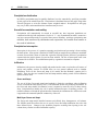
PREFACE .......................................................................................................................................................... vii
1
OVERVIEW.................................................................................................................................................1
INTRODUCTION ...................................................................................................................................................1
HISTORY .............................................................................................................................................................1
DESCRIPTION ......................................................................................................................................................2
PROCESS SIMULATED ..........................................................................................................................................2
APPLICATIONS ....................................................................................................................................................7
MODELING PROCESS ...........................................................................................................................................7
2
WATERSHED DELINEATION AND GRID CONSTRUCTION ......................................................10
INTRODUCTION .................................................................................................................................................10
OBTAINING DEM DATA FOR WATERSHED DELINEATION .................................................................................10
WATERSHED DELINEATION ...............................................................................................................................11
GRID SIZES........................................................................................................................................................13
CONSTRUCTING A GRID ....................................................................................................................................14
EDITING THE GRID TO CORRECT ELEVATION ERRORS ......................................................................................14
CONCLUSIONS ...................................................................................................................................................15
3
BUILDING A BASIC GSSHA SIMULATION ......................................................................................16
INTRODUCTION .................................................................................................................................................16
BASIC MODEL INPUTS .......................................................................................................................................16
4
ADDITIONAL MODELING CAPABILITIES ......................................................................................24
INTRODUCTION .................................................................................................................................................24
OVERLAND FLOW ROUTING OPTIONS ...............................................................................................................24
INFILTRATION ...................................................................................................................................................25
5
ASSIGNING PARAMETER VALUES TO INDIVIDUAL GRID CELLS .........................................28
INTRODUCTION .................................................................................................................................................28
INDEX MAPS .....................................................................................................................................................28
MAPPING TABLES .............................................................................................................................................30
ASSIGNING UNIFORM PARAMETERS ..................................................................................................................31
ASSIGNING SPATIALLY DISTRIBUTED PARAMETERS .........................................................................................31
6
CHANNEL ROUTING .............................................................................................................................38
INTRODUCTION .................................................................................................................................................38
LINKS AND NODES ............................................................................................................................................38
DEFINING STREAM NETWORKS WITH FEATURE LINES ......................................................................................39
LINK TYPES.......................................................................................................................................................42
SMOOTHING THE PROFILE .................................................................................................................................45
TROUBLE SHOOTING CHANNEL ROUTING PROBLEMS .......................................................................................47
iv
7
GSSHA Primer
SPATIALLY AND TEMPORALLY VARYING RAINFALL .............................................................48
INTRODUCTION .................................................................................................................................................48
TEMPORALLY VARYING, SPATIALLY UNIFORM RAINFALL ...............................................................................48
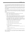
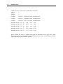
TEMPORALLY VARYING MULTIPLE-GAGE RAINFALL .......................................................................................48
8
LONG-TERM SIMULATIONS ...............................................................................................................51
INTRODUCTION .................................................................................................................................................51
GLOBAL PARAMETERS ......................................................................................................................................51
INFILTRATION MODEL.......................................................................................................................................52
EVAPOTRANSPIRATION MODEL .........................................................................................................................52
HYDROMETEOROLOGICAL DATA ......................................................................................................................54
RAINFALL DATA ...............................................................................................................................................56
9
MODELING THE UNSATURATED ZONE WITH RICHARDS’ EQUATION ...............................57
INTRODUCTION .................................................................................................................................................57
GLOBAL PARAMETERS ......................................................................................................................................57
DISTRIBUTED PARAMETERS ..............................................................................................................................59
SOIL DEPTH AND DISCRETIZATION....................................................................................................................61
10
MODELING TWO-DIMENSIONAL, SATURATED, LATERAL GROUNDWATER FLOW...62
DESCRIPTION ....................................................................................................................................................62
GLOBAL PARAMETERS ......................................................................................................................................62
DISTRIBUTED PARAMETERS ..............................................................................................................................63
BOUNDARY CONDITIONS ..................................................................................................................................64
11
SEDIMENT EROSION AND TRANSPORT .....................................................................................66
INTRODUCTION .................................................................................................................................................66
OVERLAND SEDIMENT ROUTING .......................................................................................................................66
CHANNEL SEDIMENT ROUTING .........................................................................................................................67
12
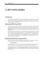
RUNNING GSSHA ...............................................................................................................................68
INTRODUCTION .................................................................................................................................................68
RUNNING GSSHA FROM WMS.........................................................................................................................68
RUNNING GSSHA FROM COMMAND LINE ........................................................................................................68
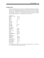
PROJECT FILE ....................................................................................................................................................69
13
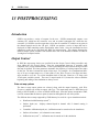
POSTPROCESSING.............................................................................................................................70
INTRODUCTION .................................................................................................................................................70
OUTPUT CONTROL ............................................................................................................................................70
VISUALIZING RESULTS ......................................................................................................................................72
REFERENCES .....................................................................................................................................................76
Table of Contents
v
Figures
Figure 1. An automatically delineated watershed boundary....................................................................... 12
Figure 2. The finite difference grid............................................................................................................. 14
Figure 3. GSSHA Job Control dialog. ........................................................................................................ 17
Figure 4. GSSHA Precipitation dialog........................................................................................................ 19
Figure 5. Example of a temporal convergence study.................................................................................. 23
Figure 6. The Index Map dialog ................................................................................................................. 29
Figure 7. The GSSHA Index Map Table Editor ......................................................................................... 30
Figure 8. Polygon coverage overlaid on a finite difference grid ................................................................ 37
Figure 9. Polygon IDs from a coverage that has been mapped to the grid cells; the grid has
been cell-fill colored according to the index map ID for each cell ............................................. 37
Figure 10. Changing diagonal stream arcs to orthogonal stream arcs. ....................................................... 40
Figure 11. Straightening small bends in the stream arcs............................................................................. 40
Figure 12. Modifying the junction location of a stream arc........................................................................ 40
Figure 13. Deleting small stream spurs....................................................................................................... 41
Figure 14. Adjusting stream arcs along cell edges...................................................................................... 41
Figure 15. Reassigning stream connections at an invalid junction. ............................................................ 41
Figure 16. The Feature Arc Attributes dialog ............................................................................................. 42
Figure 17. The stream network as a set of feature objects in WMS. .......................................................... 43
Figure 18. The (Link, Node) numbers for a stream network ...................................................................... 43
Figure 19. The Streambed Elevation smoothing editor .............................................................................. 46
Figure 20. Annual variation in canopy resistance when seasonal resistance is selected............................. 53
Figure 21. GSSHA representation of the unsaturated zone. ....................................................................... 58
Figure 22. Water retention curves, water content vs. negative pressure head ............................................ 60
Figure 23. The WMS Data Browser. .......................................................................................................... 72
Figure 24. Multiple Gage Plots................................................................................................................... 74
Figure 25. Flow depth mapped and magnified on the 2-D grid. ................................................................. 75
vi
GSSHA Primer
Tables
Table 1. Process and Approximations Techniques in the GSSHA Model..................................................... 3
Table 2. The different link types that can be used in GSSHA. .................................................................... 39
vii
Preface
The work described in this report was authorized by Headquarters, U.S. Army Corps of Engineers
(USACE). Funding for this report was provided by the Hydrologic Systems Branch, Coastal and
Hydraulics Laboratory (CHL), U.S. Army Engineer Research and Development Center (ERDC),
Vicksburg, MS. At the time of preparation, Mr. Earl Edris was Chief, Hydrologic Systems Branch, CHL,
ERDC.
This report was prepared by Dr. Charles W. Downer, CHL, ERDC, and Dr. E. James Nelson and
Mr. Aaron Byrd, Environmental Modeling Research Laboratory (EMRL), Brigham Young University
(BYU), Provo, UT.
This report was prepared under the general supervision of Mr. Edris. The report was reviewed by
Ms. Moira Fong, CH-HW, and Mr. Ryan Harrell, EMRL, BYU. Mr. Tom Richardson was Director of
CHL.
At the time of publication, Dr. James R. Houston was ERDC Director, and COL John W. Morris III,
EN, was Commander and Executive Director.
This report should be cited as follows:
Downer, C. W., Nelson, E. J., and Byrd, A. (2002). “Primer: Using Watershed
Modeling System (WMS) for Gridded Surface Subsurface Hydrologic Analysis
(GSSHA) Data Development—WMS 6.1 and GSSHA 1.43C,” ERDC/CHL TR-02-XX,
U.S. Army Engineer Research and Development Center, Vicksburg, MS.
The contents of this report are not to be used for advertising, publication,
or promotional purposes. Citation of trade names does not constitute an
official endorsement or approval of the use of such commercial products.
Overview
1
1 OVERVIEW
Introduction
This document is a primer for use of the Watershed Modeling System (WMS) interface with the
physically based, distributed-parameter hydrologic model Gridded Surface Subsurface
Hydrologic Analysis (GSSHA). The primary purpose of this primer is to describe how the WMS
interface is used to develop inputs and analyze output from the GSSHA model. This primer also
provides a brief description of the GSSHA model, including the overall model formulation,
processes that can be simulated, and input formats for files not supported by WMS.
Along with the WMS ‘how-to’ information, the primer provides hints on appropriate values to use
in a GSSHA simulation, potential problem areas, and trouble shooting suggestions. However, this
primer is not meant to be a substitute for the GSSHA User’s Manual (Downer and Ogden in
preparation), which should be consulted for specific information on the GSSHA model. Many of
the concepts used in the GSSHA model are complex, and an in-depth knowledge of the processes
involved and the solution methods available are critical for successful application of the model. It
is highly recommended that users obtain and read the GSSHA User’s Manual before attempting to
use the GSSHA model. In addition, many of the procedures outlined in this primer are described
in greater detail in the WMS Help File (Nelson 2001).
Users should be aware that the GSSHA model is always in development and is constantly being
improved, refined, and updated with new ideas. Typically, linkage with the WMS interface is the
last task completed in new model developments, after development, implementation, and testing
of the new feature in GSSHA are complete. Therefore, WMS may not support new developments
in the GSSHA model. Some files that the GSSHA model uses, such as the rainfall and
hydrometeorological data files for long-term simulations, are not supported by the WMS interface.
Files that WMS does not support are pointed out in the primer and also in the user’s manual. This
primer is meant to be used with WMS 6.1 (Nelson 2001) and GSSHA 1.43c (Downer and Ogden
in preparation).
History
The GSSHA model is a significant reformulation and enhancement of the CASC2D model (Ogden
and Julien 2002). The CASC2D runoff model originally began with a two-dimensional (2-D)
overland flow routing algorithm developed and written in a programming language (APL) by
Prof. P. Y. Julien, Colorado State University. The overland flow routing module was converted
from APL to FORTRAN by Dr. Bahram Saghafian, then at Colorado State University, with the
addition of Green & Ampt infiltration and explicit diffusive-wave channel routing (Julien and
Saghafian 1991; Saghafian 1992; and Julien, Saghafian, and Ogden 1995). The FORTRAN code
was reformulated, significantly enhanced, and rewritten in the C programming language by
Dr. Saghafian at the U.S. Army Construction Engineering Research Laboratories. This version,
named r.hydro.casc2d, was part of the Geographic Resources Analysis Support
2
GSSHA Primer
System/Geographic Information System (GRASS)/(GIS) for hydrologic simulations (Saghafian
1993). Work began in 1995 to reformulate CASC2D with the addition of continuous simulation
capabilities and ability to interface with the Watershed Modeling System graphical user interface
developed by the Environmental Modeling Research Laboratory (EMRL) at Brigham Young
University (BYU). This version, known as CASC2D for WMS, is distinguished from its
predecessors by the addition of a number of new capabilities, numerous improvements and bug
fixes, and a more stringent copyright. Johnson (1997) added overland sediment transport.
Development of the CASC2D model for WMS by the Department of Defense (DoD) ended with
version 1.18b, which has been the working distributed hydrologic model for the DoD (Downer
et al. 2002a). CASC2D Ver. 1.18b is linked with WMS 5.1 as described by (BYU 1997a and
1997b).
While developed from the CASC2D model, the GSSHA model is inherently different in that it
extends the capability of the model to simulate runoff mechanisms other than infiltration excess.
Also, input of parameters for the GSSHA model is significantly different from the methods
employed for CASC2D. The GSSHA model is backwards compatible with CASC2D Ver. 1.18b
data sets. CASC2D Ver. 1.18b, and thus GSSHA, is not necessarily compatible with prior
versions of CASC2D data sets. Also, WMS no longer supports the CASC2D input format, which
is based on providing parameter values for every grid cell through a number of floating point
GRASS ASCII format maps. When trying to utilize old CASC2D data sets, make sure they
conform to the standards described in the GSSHA User’s Manual.
Description
GSSHA is a physically based, distributed-parameter, structured grid, hydrologic model that
simulates the hydrologic response of a watershed subject to given hydrometeorological inputs.
Major components of the model include spatially and temporally varying precipitation, snowfall
accumulation and melting, precipitation interception, infiltration, evapotranspiration, surface
runoff routing, unsaturated zone soil moisture accounting, saturated groundwater flow, overland
sediment erosion, transport and deposition, and in-stream sediment transport. In GSSHA, each
process has its own time-step and an associated update time. During each time-step, the update
time of each process selected by the user is checked against the current model time. When they
coincide, the process is updated, and updated information from that process is transferred to
dependent processes. The update time or time-step of dependent processes may be modified as
part of the process update. This formulation permits the efficient simultaneous simulation of
processes that have dissimilar response times, such as overland flow, evapotranspiration (ET),
and lateral groundwater flow. This scheme also allows an integrated solution of processes
coupled through boundary conditions and flux exchanges.
Process Simulated
GSSHA is a process-based model. Hydrologic processes that can be simulated and the methods
used to approximate the processes with the GSSHA model are listed in Table 1. For several
processes, there are multiple solution methods. A brief description of the processes and solution
methods is presented. To obtain detailed information about the processes and methods, please
refer to the GSSHA User’s Manual (Downer and Ogden in preparation).
Overview
Process
Description
Precipitation distribution
Thiessen,
3
Inverse distance square weighted
Snowfall accumulation
and melting
Energy balance
Precipitation interception
Two-parameter emphirical
Overland water retention
Specified depth
Infiltration
Green & Ampt (G&A),
Multi-layered Green & Ampt,
Green & Ampt with Redistribution (GAR),
One-dimensional (1-D) vertical Richards’ equation (RE)
Overland flow routing
2-D lateral diffusive wave
Explicit,
Alternating Direction Explicit (ADE),
Alternating Direction Explicit with PredictionCorrection (ADE-PC)
Channel routing
1-D longitudinal, explicit, up-gradient, diffusive wave
Evapotranspiration
Deardorff (1977)
Penman-Monteith with seasonal canopy resistance
Soil moisture in the
Vadose zone
Bucket,
Lateral saturated
groundwater flow
2-D vertically averaged
Stream/groundwater
interaction
Darcy’s law
Exfiltration
Darcy’s law
Overland sediment
erosion
Kilinc and Richardson (1973) equation
Channel sediment routing
Yang’s method
1-D vertical Richards’ equation (RE)
Table 1. Process and Approximations Techniques in the GSSHA Model. (G&A – Green and
Ampt (1911), GAR – Green and Ampt with Redistribution (Ogden and Saghafian 1997), RE
– Richards’ equation (Richards 1931), ADE – alternating direction explicit, ADE-PC –
alternating direction explicit with prediction-correction (Downer et al. 2002b)
4
GSSHA Primer
Precipitation distribution
In GSSHA, precipitation may be spatially distributed over the watershed by specifying a number
of rain gages in the rainfall input file. Precipitation is distributed between the gages using either
Thiessen polygons or an inverse distance square weighted method. Precipitation at each gage
may vary in time, and nonuniform time increments may be used.
Snowfall accumulation and melting
Precipitation will automatically be treated as snowfall any time long-term simulations are
conducted and the dry bulb temperature is below 0 (C. Any accumulated snowfall is treated as a
one-layer snowpack that melts as a result of heat sources including: nonfrozen precipitation, net
radiation, heat transferred by sublimation and evaporation, and sensible heat transfer as
the result of turbulence.
Precipitation interception
Interception is the process of vegetation capturing precipitation and preventing it from reaching
the land surface. Interception is modeled in GSSHA using an empirical two-parameter model that
accounts for an initial volume of water that vegetation can hold plus the fraction of precipitation
captured after the initial volume of water has been satisfied. The fate of intercepted water is not
accounted for in GSSHA. The rainfall intercepted by vegetation is assumed to evaporate.
Infiltration
Infiltration is the process whereby rainfall and ponded surface water seep into the soil because of
gravity and capillary suction. In GSSHA there are two general methods used to simulate
infiltration. These are the Green and Ampt (1911) model and the Richards’ equation (1931)
models. There are also two extended Green and Ampt models, making a total of four infiltration
options to chose from.
Green and Ampt
The use of all the Green and Ampt based methods is limited to conditions where infiltration
excess, or Hortonian runoff (Horton 1933), is the dominant stream flow producing mechanism. In
the Green and Ampt model of infiltration, water is assumed to enter the soil as a sharp wetting
front. Precipitation on initially dry soil is quickly infiltrated because of capillary pressure. As
rainfall continues to fall and the ground becomes saturated, the infiltration rate will decrease until
it approaches the saturated hydraulic conductivity of the soil.
Multi-layer Green and Ampt
The Green and Ampt model described assumes an infinitely deep, homogeneous, soil column.
The GSSHA model also allows the user to specify Green and Ampt infiltration into soils with
three defined layers. Changes in the hydraulic properties resulting from layering in the soil
column always results in reduced infiltration capacity.
Overview
5
Green and Ampt with redistribution
When conducting long-term simulations, the Green and Ampt infiltration with redistribution
(GAR) can be used (Ogden and Saghafian 1997). With GAR, multiple sharp wetting fronts can
be simulated, and the water is redistributed in the soil column during nonprecipitation periods.
Richards’ equation
Richards’ equation is currently the most complete method to compute soil water movement
including hydrologic fluxes such as infiltration, actual evapotranspiration (AET), and
groundwater recharge. The use of Richards’ equation is not limited to Hortonian runoff
calculations. Richards’ equation is a partial differential equation (PDE) that is solved using finite
difference techniques. In GSSHA three soil layers, each with independent parameters for each
soil type and layer, are specified. Because the Richards’ equation is highly nonlinear, finding a
solution can be difficult and time-consuming when Richards’ equation is used to simulate the
highly transient conditions often found in hydrology, such as sharp wetting fronts and fluctuating
water table. The GSSHA model employs powerful, mass conserving methods of solving the
Richards’ equation and has been capable of simulating both soil moistures and associated
hydrologic fluxes when the proper spatial discretization is employed (Downer 2002).
Overland flow routing
Water on the soil surface that neither infiltrates nor evaporates will pond on the surface. It can
also move from one grid cell to the next as overland flow. The overland flow routing formulation
is based on a 2-D explicit finite volume solution to the diffusive wave equation. Three different
solution methods are available: point explicit, alternating direction explicit (ADE), and ADE
with prediction-correction (ADE-PC). Through a step function, a depression depth may be
specified. No water is routed as overland flow until the depth of water in the cell exceeds the
depression depth. This depression depth represents retention storage resulting from
microtopography.
Channel routing
When channel routing is specified, overland flow that reaches a user-defined stream section
enters the stream and is routed through a 1-D channel network until it reaches the watershed
outlet. Channel routing in GSSHA is simulated using an explicit solution of the diffusive wave
equation. This simple method has several internal stability checks that result in a robust solution
that can be used for subcritical, supercritical, and transcritical flows.
Evapotranspiration
Evapotranspiration (ET) is the combined effect of evaporation of water ponded on the soil surface
and contained in the soil pores, as well as the transpiration of water from plants. GSSHA uses
evapotranspiration to track soil moisture conditions for long-term simulations.
Evapotranspiration can be modeled using two different techniques, the Deardorff (1977) and
Penman-Monteith (Monteith 1965 and 1981). The Deardorff method is a simplified method used
for formulations involving only bare soil. The Penman-Monteith method is a more sophisticated
method used for vegetated areas.
6
GSSHA Primer
Soil moisture in the vadose zone
During long-term simulations, the soil moisture in the unsaturated, or vadose, zone can be
simulated with one of two methods: a simple fixed soil volume accounting method (Senarath
et al. 2000) (bucket method), or simulation of soil moisture movement and hydrologic fluxes
using Richards’ equation (Downer 2002). Evaporative demand is supplied to either method by
the ET calculations.
Lateral saturated groundwater flow
Where groundwater significantly affects the surface water hydrology, saturated groundwater flow
may be simulated with a finite difference representation of the 2-D, lateral, saturated groundwater
flow equations. The saturated groundwater finite difference grid maps directly to the overland
flow grid. The saturated groundwater zone resides below the unsaturated zone, which may be
represented with either the GAR model or the Richards’ equation model. When simulating
saturated groundwater flow, the additional processes of stream/channel interaction and
exfiltration may occur.
Stream/groundwater interaction.
When both saturated groundwater flow and channel routing are being simulated, water flux
between the stream and the saturated groundwater can be simulated. By specifying that both
overland flow and saturated groundwater flow grid cells containing stream network nodes be
considered as river flux cells, water will move between the channel and the groundwater domain
based upon Darcy’s law.
Exfiltration.
Exfiltration is the flux of water from the saturated zone onto the overland flow plane. You may
have seen a seep at a change in slope on a hillside. This seepage is exfiltration. Exfiltration
occurs when the water table elevation exceeds that of the land surface. Fluxes to the land surface
are computed using Darcy’s law.
Overland sediment erosion
Sediments on the overland flow plane can be eroded, transported, and deposited using the soil
erosion model developed by Kilinc and Richardson (1973), modified by Julien (1995) and
implemented in CASC2D by Johnson (1997). Cell to cell sediment discharge by means of
overland flow is a function of the hydraulic properties of the flow, the physical properties of the
soil, and surface characteristics. Sediment transport is computed for three grain sizes: sand, silt,
and clay. Conservation of sediment mass is used to determine what portion of sediment in a grid
cell is deposited and what portion stays in suspension. The suspended sediment may be
transported from one cell to another. If there is insufficient sediment in suspension, previously
deposited sediment is used to satisfy the erosion demand. Insufficient previous deposition results
in the erosion of the surface.
Channel sediment routing
When both channel routing and overland-flow sediment routing are simulated, sediment routing
in the channel can also be simulated. The present version of GSSHA employs Yang’s (1973)
method for routing of sand-size total load in stream channels. The routing formulation works
Overview
7
only with trapezoidal cross sections. Silt and clay size fractions are transported with the flow as
wash load. Any gains or losses of wash load, such as deposition or erosion of silts and clays
within the channels, are neglected.
Applications
GSSHA accounts for the following conditions that may be encountered when simulating
watershed hydrology:
1. Spatial variability of soil textures, land use, and vegetation that may affect parameter
values needed to simulate important hydrologic processes.
2. Spatial and temporal variability of precipitation.
3. Snowfall accumulation and melting.
4. Drainage network of arbitrary shape and cross sections.
5. Effect of soil moisture on infiltration and runoff.
6. Effect of water table on soil moisture, infiltration, and runoff.
7. Gaining and losing streams.
8. Hortonian runoff.
9. Saturated source areas.
10. Exfiltration.
11. Overland sediment movement.
12. In-stream sediment movement.
It has been verified that GSSHA, and/or the methods taken from CASC2D and employed in
GSSHA, can be used to simulate the following types of hydrologic variables:
1. Stream discharge in Hortonian basins (Doe and Saghafian 1992; Ogden et al. 2000;
Senarath et al. 2000; Downer et al. 2002a)
2. Stream discharge in non-Hortonian and mixed runoff basins. (Downer 2002; Downer
et al. 2002b)
3. Soil moistures in Hortonian basins. (Downer 2002).
4.
Sediment discharge in Hortonian basins (Johnson 1997)
Modeling Process
Application of GSSHA requires the creation of a variety of input files and grid data (or maps).
GSSHA has been coupled with WMS in an attempt to minimize the time required to create the
needed inputs. WMS is also intended to aid in model conceptualization and analysis of results.
The basic parts of the modeling process are watershed delineation and grid construction, selection
of processes to model, parameter assignment, channel routing assignment, running the model, and
postprocessing. The GSSHA User’s Manual (Downer and Ogden in preparation) provides
detailed information on the modeling process.
8
GSSHA Primer
Grid construction
GSSHA is a finite difference based model and requires a 2-D grid representation of the watershed
being modeled. Construction of this grid is the first step in the development of a GSSHA model.
WMS has a variety of tools that can be used for watershed delineation and grid generation from
digital elevation data as well as data exported from the GRASS or Arc/Info GISs.
Process selection
Once the grid is constructed, the processes to be simulated must be selected based on the needs of
the study. The processes to be simulated are selected. It is best to start with a simple model with
few processes and proceed to build more complicated models with several processes. The
GSSHA User’s Manual (Downer and Ogden in preparation) should be consulted for more
information on which processes are appropriate for which studies.
Model parameter assignment
Once the grid has been created and processes selected, model parameters governing the execution
of GSSHA must be assigned. Model parameters include global variables such as simulation time
and time-step, as well as the distributed parameters needed to simulate processes such as
interception, infiltration, and overland flow routing. WMS facilitates global parameter assignment
with dialog boxes and distributed-parameter assignment with the use of index maps and the
mapping tables.
Channel routing
Larger watersheds normally require that the 1-D channel routing option in GSSHA be used. The
channel routing method is an explicit diffusive-wave approximation. The channel network is
described with a series of channel links and computational nodes. A link is a channel segment, or
other internal boundary condition, such as a weir, comprised of two or more computational nodes.
WMS feature arcs are used to create the channel links and assign cross-sectional parameters to the
links. In order to couple the channel routing with surface runoff, GSSHA must know which grid
cells “contain” stream nodes. When WMS creates the appropriate input files, grid cells beneath
the stream arcs are identified as stream cells and their connectivity is written to link and node map
files. WMS has several tools for creating, numbering, and assigning parameters to the channel
links and nodes.
Running GSSHA
Once all necessary input for a GSSHA simulation has been prepared, the GSSHA model is run.
GSSHA is a stand-alone program that can be executed from the command line or through the
WMS interface.
Postprocessing
Results from successful GSSHA simulations may be viewed in WMS. The optional output created
by GSSHA can include time series of maps of a number of variables including: surface water
depth, infiltration rate, cumulative infiltrated depth, spatially varied rainfall, soil moistures,
groundwater heads, and others. Time series data of several variables, such as soil moisture or
groundwater head, may be output at selected points in the grid. Time series output of discharge,
Overview
9
depth, and sediment concentration can be produced at selected nodes in the channel network.
WMS has capabilities to contour, shade, and animate the results for the entire 2-D grid.
Additionally, 2-D plots of any result variable versus time can be generated for any location in the
grid. Postprocessing techniques are used to help the user determine if a solution is reasonable or
if further model modification is necessary.
10
GSSHA Primer
2 WATERSHED DELINEATION
AND GRID CONSTRUCTION
Introduction
The primary input files for a GSSHA rainfall/runoff simulation are the 2-D finite difference grid
and its’ accompanying surface elevations. The grid is a rectangular area that covers the extents of
the watershed. Individual cells whose centroid are within the watershed boundary are flagged as
“active” (a value of “1” in the watershed mask), and cells outside the boundary are flagged as
“inactive” (a value of “0” in the watershed mask). WMS can be used to automatically delineate a
watershed boundary from digital elevation data and then construct a finite difference grid with the
appropriate active and inactive flags set for individual cells.
In this chapter you will learn where to locate digital elevation data that can be used for automated
basin delineation and assignment of surface elevations for the finite difference grid. You will
also learn the basic processes used by WMS to delineate the watershed boundary and construct a
grid.
Obtaining DEM Data for Watershed Delineation
The United States Geological Survey (USGS) has converted their topographic maps into digital
elevation model (DEM) files. These files represent the land surface as a matrix (grid) of elevation
values at a given space (resolution) apart. The most commonly used maps are the 1:24,000 series
that are commonly found in a 30-m resolution, with many areas now being converted to a 10-m
resolution. In addition, the 1:250,000 map series has also been converted into 3 arc-second
(approximately 90 m) resolution DEMs. Both DEM classes have been distributed by the USGS
for a number of years. More recently free downloads are available from the World Wide Web
(www). Many other local, state, and Federal agencies warehouse and deliver these DEM
products. The EMRL at BYU has developed a single website that contains links to some of the
most common and easy to use websites for free downloading of DEM data. This website is
hosted at:
http://www.emrl.byu.edu/gsda
In addition to DEM data, this site also contains resources for locating, downloading, and
preparing land use, soil textural classification, and image data. Each topic contains basic
information, frequently asked questions, and detailed instructions for obtaining and preparing the
data to be used in WMS.
Grid Construction
11
DEM File Formats
The USGS has two different file formats. Historically, quadrangle map DEMs have been stored
in a single file using what is often referred to as the “USGS Format.” In recent years, the Federal
Geographic Data Committee (FGDC) has developed standards for sharing spatial data and most
DEMs have been converted to this format, referred to as the “SDTS Format.” WMS can import
either format, but the old-style USGS format is a little easier to work with. The SDTS is a format
defined for vector as well as raster (grid) data. Multiple files are required to define the elevation
grid with the STDS format. In the case of DEMs, many of these required files are blank or small.
The USGS DEMs often are named with a “. dem” extension while the SDTS DEM files will
contain a “. ddf” extension. When reading the SDTS DEM, any of the “.ddf” files may be
specified for the file. WMS will automatically extract the needed information from the various
files.
Besides the two USGS file formats, the Arc/Info ASCII grid is another commonly used format by
many GIS systems. If you are trying to obtain data stored in Arc/Info grid files, you must have
the grid converted to ASCII, as the binary file format is proprietary to Environmental Systems
Research Incorporated (ESRI) and unreadable by WMS. WMS also supports the DTED and
GRASS grid file formats.
Watershed Delineation
While it is possible to manually create a grid and set the active and inactive regions, it is not
recommended. Since the DEM (or other elevation data) will be used to assign elevations to the
grid cells, it is good practice to use the elevation data to automatically create a watershed
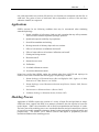
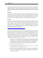
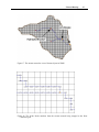
boundary. You can then use that boundary (a polygon, as shown in Figure 1) to construct a grid
that covers the watershed extents and automatically assigns cells within the boundary as active,
and cells beyond as inactive.
12
GSSHA Primer
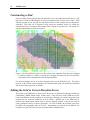
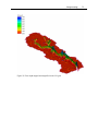
Figure 1. An automatically delineated watershed boundary through the use of a digital elevation
file and the program TOPAZ. The streams shown were also automatically created by WMS
WMS provides three methods of automated watershed delineation. An overview of each is given
here. A broader overview can be found in the WMS reference file under the Introduction chapter,
with more detailed instructions in the individual chapters. The simplest and best way to create
the watershed boundary from the DEM. Additional methods can be employed if you do not have
access to the required DEM data.
Basin delineation with DEMs
DEM data can be used in WMS to automatically delineate basin boundaries and define stream
networks. Typically a USGS DEM (multiple quadrangles can be tiled together) is imported.
Any gridded elevation data set can be used providing it is in one of the formats readable by WMS.
The United States Department of Agriculture (USDA) program TOPAZ (Martz and Garbrecht
1992) is launched from WMS to define flow directions and flow accumulations for each DEM
cell. This information is used to trace and convert the stream networks and basin boundaries to
lines and polygons of the WMS drainage coverage. The polygon and stream network shown in
the Figure 1 were delineated in WMS using this method. More details about basin delineation
with DEMs can be found in the WMS help file (Nelson 2001).
Grid Construction
13
Basin delineation with TINs
Triangulated Irregular Networks (TINs) can also be used to delineate a watershed boundary that
will be used for GSSHA models. A TIN is another form of elevation data, but rather than be
organized as a grid, rows and columns of elevations with equal spacing between, it is a network
of triangles formed from scattered elevation points. TIN data are much less common than DEM
data and slightly more complicated to work with. When using the TIN method for watershed
delineation in WMS, you should convert the resulting boundaries and stream network to feature
objects using the “Drainage Data-> Feature Objects command. Details on the use of TINs for
automated watershed delineation can be found in the WMS help file.
Basin delineation with feature objects
If you have an existing watershed boundary and stream network already defined in a GIS or CAD
environment, then it is possible to import these data in WMS as a drainage coverage and use the
imported feature arcs directly to create the GSSHA grid and channel data. However, elevation
data are still required to interpolate surface elevations to the resulting GSSHA grid. When using
an existing watershed boundary, you should use caution because, unlike the DEM method where
the boundaries and streams are defined directly from the elevations, the streams and boundary of
the imported data may not coincide with the interpolated elevation data. This can result in
elevation errors in overland flow grid cells and channel nodes, leading to numerical instability in
the GSSHA model. The elevations in the resulting grid may need to be edited on a cell by cell
basis. Further details on the use of feature objects are provided in the WMS Help File.
Grid Sizes
In general, the higher the resolution (smaller grid cells), the more accurate the solution will be.
While theoretically the number of grid cells that can be used for GSSHA modeling is unlimited,
there are some practical limitations. In order to define all model parameters, approximately
3,500 bytes of memory are required for each grid cell. This means that one megabyte of RAM is
required for each 300 grid cells of a GSSHA simulation. In addition to the amount of memory,
the time to display and work with the model inside of WMS and the time required for the GSSHA
simulation to run will increase.
The issue of appropriate grid sizes has not been adequately answered to date. Several research
papers address the range of applicability of the diffusive wave form of the equations of motion
that are used for overland flow routing in GSSHA. However, the picture is complicated by the
difficulty in including the effects of microtopography on runoff routing. Given this fact, the use
of any physically based routing technique is merely an approximation of reality. GSSHA has
been successfully used with grid sizes ranging from 30 to 1,000 m (~100 ft to 3,280 ft).
However, experience by the GSSHA developers has shown that grid sizes smaller than 200 m
(660 ft) produce more robust calibrations. Downer et al. (2002b) discuss how grid size should be
sufficiently small to capture the essential features in the study watershed. In general, the
philosophy of distributed hydrology is that “smaller is better” provided that the problem remains
computationally feasible and the quality of the data warrants the use of small grid sizes.
14
GSSHA Primer
Constructing a Grid
Once a boundary feature polygon has been defined by one of the methods described above, a 2-D
grid can be created in WMS using the Create Grid command in the Feature Objects menu. WMS
will then prompt you for the grid size and fill the interior of the rectangle that just bounds the
watershed. Each grid cell is flagged as being inside the watershed (active) or outside the
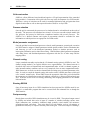
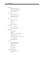
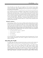
watershed (inactive) according to the location of the centroid of each grid cell. The results of a
typical grid generation are shown in Figure 2.
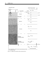
Figure 2. The finite difference grid covers the extents of the watershed. Each grid cell is flagged
to indicate whether it is inside or outside the watershed. Elevations for the cells inside the
watershed are then interpolated from the background DEM
For more information on how to use this command, please see the WMS Help File. This grid is
the heart of the GSSHA model and defines the watershed mask (grid cells within the watershed)
and elevation map required to run GSSHA.
Editing the Grid to Correct Elevation Errors
The quality of the DEM plays a major role in the success of distributed hydrologic simulations.
Unfortunately, DEMs almost always contain errors. Large flat areas in the DEM may be the
result of the limited vertical resolution of elevation data. Routing over such flat areas can create
problems for the numerical techniques used in GSSHA. Artificial pits in the DEM may be
artifacts of the interpolation scheme used to rasterize digitized contours, or may be the result of
coarse resolution in areas of concave topography. As a rule of thumb, the user must cross check
the DEM with topographic maps of the area. Interpolating elevations from the DEM at one
resolution to a grid with cells of coarser resolution induces additional error.
Grid Construction
15
One way to discover potential errors in the grid elevations is to run GSSHA with a relatively short
time-step, uniform rainfall, and simulating just the overland flow. Infiltration, channel routing
and all other model options are turned off. If the simulation terminates normally, overland depth
maps can be examined to determine where water accumulates on the overland flow plane and
whether the topographic map of the area justifies such accumulation. Alternatively, if the model
crashes at a certain location (whose address is printed on the screen as well as at the bottom of
discharge file) the user must double-check the grid elevations for problems. This process is
described in detail in the next chapter. Some manual editing of the grid elevations is almost
always necessary to impose actual drainage trends and correct obvious errors in the elevations.
Manual editing is done in WMS by selecting individual grid cells and manually typing in a new
elevation in the edit window.
Nonsmoothed grid elevations result in the need for short computational time-steps and can lead to
numerical instability problems when running GSSHA. Properly smoothed grid elevations,
particularly those with coarser grid space resolution, allow use of longer time-steps while
maintaining the stability of the model. Once overland flow is working satisfactorily, other
processes such as infiltration and channel routing can be incrementally added to the simulation.
Conclusions
The basic process used in WMS to create a grid is to first delineate the watershed boundary and
streams from a DEM and convert the results to a bounding polygon for the watershed. This
bounding polygon is then “filled” with grid elements of the appropriate size for the planned
simulation, and elevations for grid cell centers are interpolated from the original DEM. WMS
provides multiple options or creating the bounding polygon, but the recommended method is to
use a DEM. WMS supports both USGS file formats as well as Arc/Info ASCII grid files.
The size of grid cells used for a GSSHA simulation will vary depending on the area of the
watershed and objectives of the simulation, as well as computing resources. Inevitably some of
the grid cells will need to have elevations adjusted to create more “natural” and numerically
stable overland flow. The need to edit grid cells is most easily identified by running a basic
simulation to examine areas on the grid that pond excessively. Setting up and running a basic
simulation is the content of the next chapter.
16
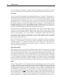
GSSHA Primer
3 Building a Basic GSSHA Simulation
Introduction
A complete GSSHA simulation may include temporally and spatially varying rainfall for multiple
events over an extended period, distributed roughness parameters, infiltration modeling with
distributed parameters, channel routing, and saturated groundwater flow with stream interaction.
However, such a simulation is built in pieces, not all at once. A simple simulation is constructed,
problems are corrected, and then additional processes or inputs are added, one at time. The key is
to successfully build a simple simulation, and then build upon your success.
The most basic simulation is built through four steps:
1. Assigning elevations to each cell, as described in Chapter 2.
2. Assigning the values of a limited number of global parameters.
3. Describing the uniform rainfall event.
4. Assigning uniform value of overland flow roughness.
Once this simple simulation works, processes or complexities, as described in the following
chapters, are added. The information in this primer is presented in the order that complexities
should be added. The new simulation, with added complexity, should be tested before adding
more complexity to the simulation. This process of building a simulation is described in detail in
the GSSHA User’s Manual.
Basic Model Inputs
Global parameters
The global parameters of a simulation refer to the input control and other parameters not assigned
on a cell-by-cell basis; e.g., the numerical method for computing overland flow, the computational time-step and total simulation time, and whether to activate certain model options such as
channel routing, long-term simulations, infiltration, evapotranspiration, groundwater interaction,
etc.
The Basic Simulation
17
To have WMS allocate the memory required for development and storage of GSSHA model
parameters, you must first initialize a simulation. This is usually done when creating a grid,
because WMS prompts the user whether or not to do so. However, the simulation parameters can
be initialized or deleted using the identified buttons in the GSSHA Job Control Parameters
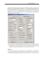
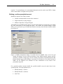
dialog. Data necessary to run a GSSHA simulation are determined based on the settings in the
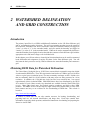
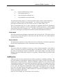
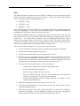
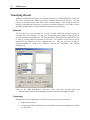
GSSHA Job Control Parameters dialog (Figure 3). A better description of the various options is
provided in the next several sections.
Figure 3. GSSHA Job Control dialog in WMS. This dialog is used to select model options and
global parameters needed by GSSHA. The Output Control dialog, accessible from the Output
Control button in the lower left-hand corner, is used to indicate the desired time-series maps
that GSSHA can output, such as the depth of water on the overland flow plane.
Total time
The total time parameter sets the total simulation time for a model in minutes. If the falling limb
of the discharge hydrograph is of particular interest, the total simulation time must be set to a
value greater than total rainfall duration plus the expected recession time. The total time is used
18
GSSHA Primer
only for single-event simulations. During long-term simulations, the total time is not used
because the simulation time is determined from the rainfall and hydrometeorological input files.
Time-step
The time-step ('t) is the duration of the computational time-step, in seconds. The time-step is a
critical variable in determining the wall clock execution time for a simulation. Typical time-steps
for GSSHA simulations range from 20 sec up to 5 min. For particularly hard problems, the timestep may need to be very short, 10 sec, 5 sec, or even less. One second (1 sec) is the smallest
permissible time-step. The overall model time-step must be less than, and integer divisible into
the smallest increment of time in the rainfall file. For example, for 1-min rainfall data the
maximum time-step is also 1 min. Other permissible values would be 30, 20, 10, 5, 2, and 1 sec.
If saturated groundwater flow is being simulated, then the overall model time-step must also be
equal to or less than, and integer divisible into, the groundwater time-step.
The general rule for overland routing is that shorter time-steps must be used for higher intensity
storms, finer horizontal grid resolution (grid spacing, 'x), steeper watershed slopes, larger
watershed areas, and smoother surfaces. Stability of the explicit routing routines depends in part
upon the Courant number. The Courant number is a dimensionless number that expresses the
wave celerity, water velocity for steady flows, over the model celerity, 't/'x. For model
stability, the Courant number must be less than 1.0; that is, water should not move more than one
grid cell during a single time-step.
Shorter time-steps must be used when backwater effects are significant, which occurs mainly in
flat areas. If the time-step is too long, the surface water depth in flat areas may show a
checkerboard pattern, i.e., oscillations are observed in the water surface level. In such cases, the
time-step should be decreased and the simulation repeated. Alternately the flat areas can be
removed by editing the elevations.
Outlet information
When channel routing is not specified, information about which cell represents the watershed
outlet and the slope of the land surface at the outlet must be defined. The outlet location is input
as the row and column (I and J indices). The user must ensure that the outlet described by its row
and column is within the active area of the watershed mask. The bed slope is equal to the tangent
of the angle that is made between the bed profile at the outlet and the horizontal plane. This slope
is used to calculate the outflow overland discharge at the outlet based on a normal depth
boundary condition. When channel routing is specified, the outlet of the catchment is defined by
the location of the stream network, and the grid cell that contains the outlet need not be specified.
Units
The units flag in WMS is used to identify whether the grid dimensions and elevations are in feet
or meters. GSSHA is entirely formulated in metric units. When English units are specified, the
grid dimensions and elevations are converted to metric inside of GSSHA. For instance, the UTM
coordinate system uses meters for the X,Y coordinates. The user should verify that the elevation
(Z) coordinates are also in meters. It is not possible to use a mixed unit system in GSSHA. The
grid size and elevation data must be in the same unit system. When using UTM coordinates, the
units flag should be set to metric. The State-Plane coordinate system, on the other hand, uses feet
for the X,Y dimensions. The elevation values in State-Plane maps should also be in feet, and the
units flag should be set to English to inform GSSHA that the conversion from feet to meters is
The Basic Simulation
19
required. To avoid problems, it is recommended that metric units be used to run GSSHA. Output
units of either Metric or English can be specified.
Defining a uniform precipitation event
Rainfall can input in one of three formats:
x Uniform constant rainfall over the entire watershed.
x Single temporally varying rain gage.
x Multiple, temporally varying rain gages.
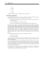
All rainfall types in GSSHA must be tied to a specific point in time by specifying the year, month,
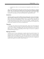
day, hour, and minute of each rainfall data point. The GSSHA Precipitation dialog in WMS
allows you to specify the type of rainfall and enter the necessary data associated with the rainfall
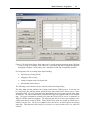
type (Figure 4).
Figure 4. GSSHA Precipitation dialog. Accessible from the GSSHA menu in the 2-D grid
module, this dialog is used to define precipitation events. WMS currently supports only the
capability to simulate a single-gage event or uniform precipitation. Precipitation patterns that
include multiple gages and/or multiple events must be developed in a text editor external to
WMS. See the GSSHA User’s Manual for more information on the format of the
precipitation input file
For a spatially uniform constant rainfall, the specified rainfall covers the entire basin for the
specified period. The input parameters are:
x Rainfall Intensity - (mmh-1).
x Rainfall Duration - (minutes).
x Start Time.
20
GSSHA Primer
1. Year
2. Month
3. Day
4. Hour
5. Minute
Temporally and spatially varied precipitation is discussed in Chapter 7.
Describing overland flow
The computational method used to compute overland flow is selected in the GSSHA Job Control
Parameters dialog from Overland flow sim. Three methods are available.
x Explicit – original point explicit method developed for CASC2D, as described by Julien
and Saghafian (1991).
x ADE – alternating direction explicit (Downer 2002).
x ADE-PC – alternating direction explicit with prediction-correction (Downer 2002).
The default value is Explicit. The ADE and ADE-PC methods are described in the GSSHA
User’s Manual. Generally, the ADE method is recommended. The ADE method will usually out
perform the original Explicit method, and a larger time-step may be used without affecting the
hydrograph shape. The ADE-PC method is the most robust and may be employed when
particularly difficult conditions are encountered. The ADE-PC method will often work when the
other two methods will not. The additional computations in the ADE-PC method make it
significantly slower than the other two methods, which require about the same wall clock time.
Some experimentation may be required to determine which method will work best for a particular
problem.
The following inputs are required in overland flow simulations in GSSHA.
x Land surface elevation.
x Land surface roughness.
The grid cell land surface elevations (determined from the DEM, as discussed in Chapter 2) and
the surface roughness comprise the minimum input parameters that must be defined for a GSSHA
surface runoff simulation.
The surface roughness represents the overland Manning’s roughness coefficient n. These values
can be spatially distributed using an index map defined from vegetation cover and/or land use.
Values of overland roughness coefficients based on vegetation coverage are presented by Engman
(1986) and Ree, Wimberly, and Crow (1977), and summarized in the GSSHA User’s Manual
(Downer and Odgen in preparation).
By using Manning’s resistance equation, it is assumed that the overland flow is turbulent flow
over rough surfaces. Manning’s roughness coefficients are dimensionless. Assignment of
parameter values to every grid cell is discussed in Chapter 5.
The Basic Simulation
21
Verifying the basic model
For every new GSSHA model a basic simulation with uniform roughness should be run to
determine the overall quality of overland flow. The minimum parameters that must be defined to
run a basic simulation are surface roughness and rainfall. As described above, the time-step, total
time, and outlet information must also be defined. The required steps are described below.
1. In the GSSHA Job Control Parameters dialog, make sure that all optional processes
(routing, sediment, infiltration, etc.) are turned off. Enter a value for total simulation
time in minutes (a few hours) and a small time-step in seconds (5 to 10 sec). In the
GSSHA Job Control Parameters dialog, select Output Control, toggle on Surface depth
under the Data Set Map Options. Toggle on the ASCII map Type. Input a Write
Frequency (time-steps) such that maps of surface depth are written out every 15 to
30 min, about 90 to 180 time-steps.
2. For the uniform rainfall event, enter an intensity of 10 to 50 mmhr-1 and a duration of
1 to 2 hr (60 to 120 min).
3. Assign a uniform overland roughness coefficient, as described in Chapter 4, with a value
of 0.05.
4. Save the project and run GSSHA.
The model should run to completion and produce a hydrograph at the outlet. If the model runs
but does not produce flow at the outlet, then either increase the total time of your simulation, your
rainfall duration, or your rainfall intensity and rerun the model. Do this until there is output. The
model may or may not run to completion as flow is produced.
If the model does run to completion, use the methods described in Chapter 13, Postprocessing, to
view the outlet hydrograph and the overland flow depth maps. These maps are useful for locating
problem areas in the watershed and comparing areas of ponded water to independent topographic
data. If water is ponded on the watershed at the end of the simulation (ponded water shows up as
blue areas on the overland flow depth maps), compare these locations to topological maps and
ensure that the ponded areas correspond to real depressions. If these areas should drain, you may
have to go back and do more smoothing on the DEM or manually edit the values of elevation in
the affected grid cells, as discussed in Chapter 2. Even if the ponding areas correspond to natural
depressions, you may still wish to smooth the DEM or edit the grid elevations to drain these
areas, as computation of overland flow with significant backwater effects requires a small timestep. Experience has shown that DEM smoothing has minimal effect on streamflow predictions.
If the overland flow routine crashes, information on problem areas will be printed to the screen
and also to the run summary file. If the overland flow module will not run you can try to change
the overland flow routing method to ADE-PC, reduce the time-step, or decrease the uniform
rainfall intensity or duration. If the model will not run with a small time-step and the very stable
ADE-PC overland flow routine, the depth maps should be consulted to identify potential
problems in the watershed. The DEM may be smoothed using algorithms in the WMS software,
or the elevations in the grid may also be manually edited. The information provided by GSSHA
will tell you where to target editing of grid cell elevations. Zoom in on these identified problem
areas; turn on the color fill contours, and display the grid cell elevations. You may have to
remove flat spots, dams, or depressions that are causing the overland flow model to crash. If
water is ponding along the edge of the watershed, these cells will either have to be removed from
the grid or raised in elevation. Another potential solution to making the overland flow module
22
GSSHA Primer
run is to increase the grid size, which will reduce the Courant number and smooth the elevations
in the model.
Determining an appropriate time-step
A good way to determine the appropriate time-step for a given problem is to conduct a temporal
convergence study. Select from the study period a rainfall event of the highest rainfall intensity,
or the one that produces the maximum discharge. Select a short time-step, 5 to 20 sec, and
simulate the event. Write out the discharge hydrograph at small intervals, equal to the time-step.
Increase the time-step and repeat. Continue increasing the time-step until the program crashes
during execution. At this point, the upper limit of the time-step for your problem has been
reached. Look at the hydrographs produced using the various time-steps. If the hydrograph
begins to oscillate, normally near the peak, the time-step is too large. Eliminate any simulations
that produce oscillations in the hydrograph.
There should now be a set of hydrographs produced by various time-steps. As the time-step is
increased, the hydrograph shape may begin to change. A primary theory of the finite difference
method is that the model results converge on the solution as the time-step decreases. Therefore,
the hydrograph with the smallest time should be treated as the “correct” answer, and the other
hydrographs should be judged against it. A simple visual comparison of the hydrographs is
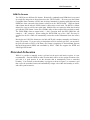
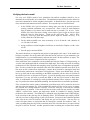
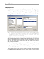
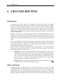
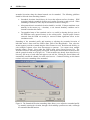
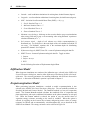
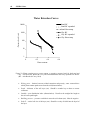
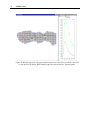
usually sufficient. Figure 5 shows the hydrographs produced from a test case with time-steps of
10, 150, 180, and 210 sec. At 150 sec, the hydrograph is significantly shifted from the 10-sec
simulation. At 180 sec, oscillations appear. At 210 sec, the oscillations cause the model to crash.
All these time-steps are too large. The simulation time-step may also be judged by the peak
discharge, time of peak, and discharge volume information from the summary file. To decrease
wall clock execution time, select the largest time-step that produces results equal to, within an
acceptable error level, the results with the smallest time-step.
The Basic Simulation
23
Figure 5. Example of a temporal convergence study. The hydrograph produced by the 10-sec
time-step can be considered the most correct because it has the shortest time-step. The
210-sec time-step hydrograph crashed partway through the run. The 180-sec time-step, shows
the oscillations that will be produced by a time-step too close to the limiting or crashing timestep. The 150-sec time-step appears normal, but when judged against the 10-sec time-step, the
significant difference in peak time is observed, making the 150-sec time-step also
inappropriate
24
GSSHA Primer
4 ADDITIONAL MODELING
CAPABILITIES
Introduction
As described in Chapter 1, there are many modeling options in GSSHA beyond the basic overland
flow model described in Chapter 3. This chapter summarizes and describes the additional
modeling options in GSSHA. More detailed descriptions of some modeling options are offered in
following chapters, as needed. The processes GSSHA simulates to predict streamflow may
include overland flow, spatially and temporally varied rainfall, infiltration, and channel routing.
It is typical to use the long-term model to conduct simulation calibration or to simulate extended
events. Modeling of the unsaturated zone with Richards’ equation and saturated groundwater
modeling may be required in areas where infiltration-excess runoff is not the predominate streamflow producing mechanism. Sediment routing is an additional capability used in studies
specifically designed to compute sediment loads.
Overland Flow Routing Options
GSSHA offers several optional processes that can be selected along with the basic overland flow
routing described in Chapter 3. These optional processes are selected in the GSSHA Job Control
Parameters dialog box under Surface Flow. Toggle on the desired options and then supply the
needed inputs as described below. The optional processes are:
x Interception.
x Initial Depth.
x Area Retention.
x Retention Depth.
Interception
Interception is defined in GSSHA using two distributed parameters: an interception coefficient
(b) and a storage capacity (a). The interception rate (i) is expressed as:
i(t) = r(t)
while I <= a
i(t) = b * r(t)
while I > a
Additional GSSHA Capabilities
25
where:
r(t)
denotes rainfall intensity at time t
a
is the storage capacity, m
b
is the interception coefficient, ms-1
I
is the cumulative interception depth
The interception storage capacity, a, must be specified in units of meters, and the interception
coefficient, b, must be in units of meters#seconds-1. For a table of storage capacity and
interception coefficient values, see Gray (1970), section 4.6, or Bras (1990), p 233.
These two parameters may vary in space, depending on vegetation and land use distributions.
The storage capacity parameter, as well as interception coefficient parameter, is usually created
from an index map of the vegetation cover. Typically, interception is not simulated in GSSHA;
the effects of interception are included in the surface retention and infiltration parameters.
Initial depth
This value represents the beginning overland depth value in the grid cells. This feature is rarely
used, since the overland flow plane is usually dry prior to the first storm event. Initial depths are
specified in units of meters.
Area reduction
This dimensionless fraction is used to reduce the area over which there is infiltration opportunity
after the end of rainfall because of flow concentration in micro-topography.
Retention
This feature allows the simulation of storage as a result of micro-topography. If the depth of
water in a grid cell is less than the retention depth, no overland flow is routed. This feature has
the effect of increasing the amount of infiltration. The retention depth is specified with the
Mapping Table tied to index maps of land use or vegetation. Retention depth is specified in units
of millimeters.
Infiltration
GSSHA provides two basic methods and four different options for simulating infiltration. The
two basic methods are the Richards’ equation, described in Chapter 9, and the Green and Ampt
method (1911), as described below. Selection of Richards’ equation over one of the Green and
Ampt methods actually results in the model operating quite differently, most notably during longterm simulations (Chapter 8). There are three Green and Ampt methods; basic Green and Ampt
(1911), Green and Ampt with Redistribution (GAR) (Ogden and Saghafian 1997), and multilayer Green and Ampt (Downer and Odgen in preparation). The multi-layer Green and Ampt
model is not currently supported by WMS, and the user is referred to the GSSHA User’s Manual
for more information on this option.
In the Job Control dialog, one of four choices can be specified:
26
GSSHA Primer
x No infiltration.
x Green & Ampt.
x Infiltration redistribution.
x Richard’s infiltration.
If no infiltration method is specified, then no parameters need be defined. If Green & Ampt is
chosen, then grid parameters of soil hydraulic conductivity, porosity, wetting front suction head
(capillary head), and initial moisture content must be defined. If the infiltration with
redistribution option is chosen, the pore distribution index and residual saturation must also be
defined. Selection of Richards’ equation requires the user to specify both global parameters and
distributed grid cell parameters, as described in Chapter 9.
Green & Ampt infiltration
In the Green and Ampt model of infiltration, water on an overland flow grid cell resulting from
precipitation, overland flow, or other sources is assumed to enter the soil as a sharp wetting front.
The soil behind the front is assumed to be saturated. The soil ahead of the front is assumed to be
at some uniform initial moisture. The wetting front is drawn into the soil because of gravity and
soil capillary pressure. As the front moves into the soil column, the effect of the soil capillary
head is reduced and infiltration slows, approaching the value of the saturated hydraulic
conductivity.
Four soil property parameters are required for each cell:
x Saturated hydraulic conductivity (cmhr-1).
x Wetting front suction head or capillary head (cm).
x Porosity - fraction of voids in the soil (dimensionless).
x Initial moisture content - initial fraction of water in the soil (dimensionless).
The first three parameters may be assigned based on an index map of soil textures. As the land
use may also affect these parameters, it is typical to create a composite land use/soil texture index
map to assign these parameters. In the absence of measured field data, the parameters may be
estimated based on the soil textural classification. Tables of parameters can be found in Rawls,
Brakensek, and Saxton (1982) and are summarized in the GSSHA User’s Manual (Downer and
Ogden in preparation). Assignment of these parameters based on soil textural classification
typically requires that one, some, or all of these parameters be adjusted during calibration.
The initial moisture content must be less than or equal to the porosity and should be greater than
the residual water content. Estimation of the initial soil moisture is based on antecedent conditions in the watershed. The Green and Ampt method is highly sensitive to the value of initial
moisture. Accurate initial moisture estimates are required. Initial moisture estimates may be
determined from field measurements, satellite measurements, or may be provided by the GSSHA
model when long-term simulations are conducted (Chapter 8). Senarath et al. (2000) demonstrate
the dangers of using initial moisture as a calibration parameter in single event calibrations.
Redistribution
When GAR is selected for modeling infiltration, soil pore water is redistributed during periods of
no or low-intensity rainfall, and infiltration capacity recovers for the next burst of storm intensity.
Additional GSSHA Capabilities
27
The technique used for hiatus and posthiatus stages is based on the method by Smith, Corradine,
and Melone (1993) with minor modifications (Ogden and Saghafian 1997). In this model, the
Green & Ampt equation is used for posthiatus stage, so the four Green & Ampt parameters must
be specified. In addition, the pore size distribution index (dimensionless) and residual saturation
(dimensionless) are required. Without field measurements, values for these parameters may also
be estimated bases on soil textural classifications and assigned from literature values, e.g. Rawls,
Brakensek, and Saxton (1982) and summarized in the GSSHA User’s Manual (Downer and
Ogden in preparation).
Richards’ infiltration
When Richards’ equation is specified for simulation of infiltration, the movement of water in the
soil is explicitly solved using Richards’ equation (Richards 1931). Detailed soil moisture profiles
are calculated in each overland grid cell with infiltration calculated as a by-product of the
solution. Richards’ equation requires many of the same parameters described above, in addition
to global parameters related to the solution techniques used in the model. Richards’ equation and
the proper assignment of parameters are described in detail in Chapter 9.
Channel routing options
One-dimensional channel routing can be coupled with overland flow routing by turning on the
channel routing option. A channel network, complete with geometric cross sections and other
parameters, must be defined. Details of defining channel routing parameters for GSSHA using
WMS are discussed in Chapter 6.
Long-term simulations
Long-term simulations can be used to simulate multiple rainfall events that occur over an
extended time period. The effects of wetting and drying of the soils in the watershed are
simulated. Long-term simulations require many additional inputs as detailed in Chapter 8.
Subsurface
Subsurface simulations can be performed to simulate the lateral flow of saturated groundwater
movement and interactions with surface water. The 2-D free surface equation (Pinder and
Bredehoeft 1968) is solved using finite difference techniques (Trescott and Larson 1977; Downer
2002). Selecting this option requires the assignment of appropriate boundary conditions and
parameters to define the groundwater media. Details of simulating saturated groundwater are
discussed in Chapter 10.
Soil erosion
Soil erosion and sediment transport can be simulated on the overland flow plane using the Kilinc
Richardson equation (Kilinc and Richardson 1973). Selecting overland soil erosion requires that
appropriate soil parameters be defined for each grid cell. Channel sediment routing can also be
simulated if both the overland flow sediment routing option and channel routing options are
specified. Yangs’ method (Yang 1973) is used to route sand as bed load. Silt and clay are routed
as wash load (Ogden 2000). Details for setting up soil erosion and sediment transport simulations
are discussed in Chapter 11.
28
GSSHA Primer
5 ASSIGNING PARAMETER
VALUES TO INDIVIDUAL GRID
CELLS
Introduction
As described in the preceding chapters, the simulation of many processes requires that parameter
values be assigned to every cell in the active watershed grid. GSSHA can accept parameter values
for every cell as a specified uniform value, as a GRASS ASCII map with a different value for
every cell, or as tabled values referenced to index maps. In WMS, parameters are assigned to cells
by using the mapping tables and index maps. Index maps are maps that assign integer ID values
to every cell in the active watershed area. Index maps for distributed parameters are usually
based on soil texture, land use, and vegetation classifications. Parameter values are assigned to
each cell based on its index number. A table of parameter values is created for each process and
assigned an index map.
Index Maps
An index map is an array of integer values (one for each grid cell) that represent unique IDs for
the different spatially distributed properties being defined. The typical maps (although not
restricted to) are derived from:
x A land use (land cover or vegetation cover) coverage.
x A soil texture coverage.
x A combination of land use and soil type coverages where all the combinations of land use
and soil texture are determined with an ID created for each unique pair of overlapping
polygons.
The Index Maps dialog is used to create and manage different index maps used in WMS. This
dialog is shown in Figure 6.
Model Parameter Assignment
29
Figure 6. The Index Map dialog. Index maps can be created through generating unique IDs from
a GIS coverage or coverages, such as land use, or the entire map may be assigned a single ID
through the Constant->Array button. Also, individual cell IDs may be manually modified
Several options exist for creating index maps including:
x Importing an existing grid file.
x Mapping a GIS coverage.
x Setting a constant value for all grid cells.
x Interpolating from a data set.
The following sections describe the key elements of the Index Maps dialog.
The Index Maps window contains a list of maps created for the GSSHA project. A new map can
be created using the Add Map button, and the Rename Map button can be used to give it a more
meaningful name. The Copy Map and Delete Map buttons can also be used to add or delete maps
from the list. The Import button allows a GRASS ASCII grid to be imported and used as an index
map. The Import command is primarily used when the GRASS GIS is used as a companion to
WMS for GSSHA model development. The imported grid must be of the same resolution as the
GSSHA grid already created in WMS. Unless both of these grids are created in GRASS, this is
unlikely to be the case. The Export command can be used to save an ASCII grid of the selected
index map. This function is most useful if you wish to view the grid with ArcView or other GIS
software.
30
GSSHA Primer
Mapping Tables
Mapping tables are used to relate index map IDs to parameter values. The required values
depend on which simulation options are selected. The most basic value is surface roughness, but
if infiltration, evapotranspiration, or other options are defined then the parameters for each of
those options will also need to be defined. The mapping table editor, shown in Figure 7, is
accessible by selecting the Mapping Tables… command from the GSSHA menu, or by using the
Edit Mapping Tables… button in the index map dialog.
Figure 7. The GSSHA Index Map Table Editor. Each active process should be assigned an index
map, and parameter values assigned to the generated IDs. The index maps along with the
mapping tables provide the means to quickly and easily distribute the spatially varied
parameters across the 2-D finite difference grid
The GSSHA Index Map Table Editor, shown in Figure 7, allows you to select a process, generate
table IDs for that process, and define the parameter values for the IDs of the table. If you try to
select a process (evapotranspiration, for example) that has not been enabled in the Job Control
dialog, you will be prompted to turn on that option if you wish to define parameter values for the
IDs. Each active process must be associated with an index map, assigned from the Assigned
index map drop-down combo box.
The Generate IDs from map button will generate a new table ID from each unique ID in the map.
You can also Add or Delete a given ID using the appropriate buttons. To define parameter values
for a given ID, you should select that ID from the ID window. Edit the corresponding values for
that process by selecting the appropriate line in the Selected ID Property window and change the
value in the edit field just below it.
You can export a table for later use if you have a certain set of parameter values that correspond
to a standard classification system of soils or land use. This table can then be imported for use in
the development of other GSSHA models.
Model Parameter Assignment
31
Assigning Uniform Parameters
Uniform values are assigned from the Index Maps command in the GSSHA menu. Using this
dialog, a new index map can be created, and then the Constant to Array button used to assign a
single ID number to every cell in the active grid. This uniform index map may then be assigned
to any given process. The uniform index map could be assigned for overland roughness in the
following manner. Select the Edit Mapping table button. Select Roughness from the process list
and the uniform index map from Assigned index map. ID numbers may be automatically
generated from the index map by selecting the Generate IDs from map button. Alternatively,
hitting the Add ID button will also generate IDs, but in a numerically sequential order. Parameter
values for each ID are entered by selecting the ID number under ID and then filling in the
information in the Selected ID property table, which will be Surface roughness in this example.
Select Done when finished.
Assigning Spatially Distributed Parameters
One of the greatest assets of distributed hydrologic models like GSSHA is the ability to spatially
distribute the parameters for processes, such as overland flow and infiltration, over the watershed.
Assigning values, grid cell by grid cell, is tedious and makes all but the simplest and smallest
models impossible. Using WMS, GIS coverages (layers) representing land use and soil texture
can be used to assign model parameter values to groups of grid cells sharing the same
characteristics.
The basic process of assigning spatially distributed parameters consists of the following steps:
1. Import a GIS coverage for land use, soil texture, or vegetation type (generally this should
be in the ArcView shapefile format).
2. Map the land use, soil texture, or vegetation ID to the grid cells using a spatial overlay
operation.
3. Define parameter values (e.g., surface roughness, hydraulic conductivity, etc.) for the
unique ID numbers.
A given soil texture/land use (STLU) index map can be used to assign multiple parameters. Since
most of the grid cell parameters can be referenced to either land use or soil properties, a given
simulation generally requires only a single index map of each. A combination land use and soil
texture index map makes it possible to relate a parameter value to the combination of land use and
soil texture (for example infiltration or erosion). Once the index maps are defined, parameter
values are assigned to the IDs of the index maps. The combination of the index maps, with ID
numbers, and the mapping tables, with the parameter values, are used by GSSHA to internally
assign parameter values to each grid cell.
Locating GIS data
The ability to locate and obtain relevant land use and soil texture data is an important part of
assigning parameter values to a GSSHA simulation. The World Wide Web is an excellent
resource for obtaining data and the WMS developers have created a web site summarizing the key
nation-wide (US) data available for download.
This web site, maintained at
http://www.emrl.byu.edu/gsda, is updated on a periodic basis. It should be noted that the gsda
web site references data sources are maintained and distributed on a nation-wide basis. More
32
GSSHA Primer
accurate (higher resolution and more recent) data are often available from local government
agencies and universities, so it is wise to check for alternative data sources. Elevation data in
either USGS Format or Arc/Info ASCII grid, as described in Chapter 2, should be requested.
Vector coverages representing land use and soil texture should be requested in ArcView shapefile
format.
Elevation
Elevation data are essential for delineating the watershed and establishing the initial elevations in
the finite difference grid. The gsda web site contains many excellent sources of elevation data
throughout the United States and related territories. The WMS reference manual contains more
detailed information on importing, displaying, and manipulating DEM data. Chapter 2 of this
primer discusses the use of a DEM to delineate a watershed and establish the numerical grid.
Land use
The USGS provides land use classifications for the entire United States at 1:250,000 scale. These
data are available from the USGS directly, but in a format called GIRAS, not directly readable by
WMS. Arc/Info is required to convert the GIRAS data to a form useable by WMS. The
Environmental Protection Agency (EPA), as part of the BASINS program, has converted the
GIRAS files to ArcView shapefiles. These data can be downloaded from the EPA, as directed on
the gsda web site, and used directly in WMS. A list of land use code descriptions can be read
from the Appendix at the following USGS site:
http://edcwww.cr.usgs.gov/glis/hyper/guide/1_250_lulc
A link to this location can also be found in the gsda web site.
The land use maps downloaded from the EPA site are organized by the USGS 1:250,000 maps.
These maps are generally large relative to the size of the watershed being modeled and can tax
WMS’s memory resources. It is suggested that you use ArcView or other GIS software to clip out
the region of interest. For example: after delineating the basin as described in Chapter 2, export
the basin boundary polygon as a shape file. You can then use the GeoProcessing extension
within ArcView to clip out the land use that covers the area of interest. You can also simply make
a bounding box that is bigger than the watershed and use it to clip out the desired data. The
following lists some details for using ArcView to do this.
x Follow the links on the EMRL gsda website to the EPA basins data and download the
required data for your watershed. These data will include both the USGS Land Use/Land
Cover data on the 1:250,000 map scale and the Natural Resources Construction Service
(NRCS) Statsgo soil data clipped by watershed Hydrologic Unit Classification (HUC).
x From your delineated watershed in WMS, export the basin boundary as a shapefile.
x Load the basin boundary shapefile into ArcView.
x Load the land use data downloaded for your watershed (often there are multiple
1:250,000 map sheets for a given HUC) into ArcView.
x The land use data are in geographic (lat/lon) coordinates, while your boundary is likely in
Universal Transverse Mercator (UTM) or some other planimetric coordinate system.
You will need to “project” one or the other data sets so that they are consistent. The
following is recommended.
Model Parameter Assignment
33
o
ArcView contains tools for projecting shapefiles. The latest version 8.0 has a
projection wizard, but there is also a simple tool in the sample extensions called
the “projector.” This extension will add a little button to your macros.
o
Using the ArcView projection tools, change the land use data from geographic
coordinates to the coordinate system of your watershed.
o
If your watershed overlaps multiple land use maps, you will need to project all of
them.
o
While it is possible to use the WMS coordinate conversion (projection) tools, this
method requires two conversions. First, the boundary must be converted to
geographic coordinates before exporting. The land use and soil data must also be
converted from geographic to your working coordinate system after importing.
In ArcView only one conversion is required.
x Make sure the geoprocessing wizard extension is on in ArcView.
x Using the Clip command in the geoprocessing wizard, clip the land use data using the
watershed boundary polygon.
x If you have multiple land use maps, you will need to clip both and then merge the results
(or merge the maps before clipping).
x The clipped land use file can now be imported to WMS as a Land Use type coverage
where the LU_CODE attribute is mapped as the WMS Land Use data.
x Make an index table with matching attributes for the GSSHA model based on the
LU_CODE parameters. The EMRL gsda website includes a link to the USGS land use
information describing the different land use codes. That index table is reproduced here:
Classification codes 1 Urban or Built-Up Land
11 Residential
12 Commercial Services
13 Industrial
14 Transportation, Communications
15 Industrial and Commercial
16 Mixed Urban or Built-Up Land
17 Other Urban or Built-Up Land
2 Agricultural Land
21 Cropland and Pasture
22 Orchards, Groves, Vineyards, Nurseries
23 Confined Feeding Operations
24 Other Agricultural Land
34
GSSHA Primer
3 Rangeland
31 Herbaceous Rangeland
32 Shrub and Brush Rangeland
33 Mixed Rangeland
4 Forest Land
41 Deciduous Forest Land
42 Evergreen Forest Land
43 Mixed Forest Land
5 Water
51 Streams and Canals
52 Lakes
53 Reservoirs
54 Bays and Estuaries
6 Wetland
61 Forested Wetlands
62 Nonforested Wetlands
7 Barren Land
71 Dry Salt Flats
72 Beaches
73 Sandy Areas other than Beaches
74 Bare Exposed Rock
75 Strip Mines, Quarries, and Gravel Pits
76 Transitional Areas
77 Mixed Barren Land
8 Tundra
81 Shrub and Brush Tundra
82 Herbaceous Tundra
83 Bare Ground
84 Wet Tundra
85 Mixed Tundra
9 Perennial Snow and Ice
91 Perennial Snowfields
92 Glaciers
Model Parameter Assignment
35
Soils
The Natural Resources Conservation Service (NRCS), formerly the Soil Conservation Service
(SCS), has created a comprehensive set of soil coverages. These can be found at three different
scales. From least detailed to most detailed they are:
x NATSGO - nation
x STATSGO - state
x SSURGO - county
The STATSGO data have been compiled in ArcView shapefile format by watershed units (large
basins) for distribution as part of the EPA BASINS program. Detailed information for
downloading STASGO data is provided on the gsda web site.
The NRCS also distributes the files on a state-by-state basis. The state files are very large. For
many states the files are too big to read into WMS without clipping, as suggested in the Land Use
section above. A secondary table containing various soil classification information must be
joined to the polygons using ArcView prior to using in WMS. The name of this table is
“comp.dbf” and should be joined with the polygons based on the MUID field name (present in
both the feature attribute table of the polygons and the “comp.dbf” file).
The necessary details for using ArcView to process the soils data follows:
x From your delineated watershed in WMS, export the basin boundary as a shapefile.
x Load the basin boundary shapefile into ArcView.
x Load the soils data downloaded for your watershed into ArcView.
x The soils data are in geographic (lat/lon) coordinates, while your boundary is likely in
UTM or some other planimetric coordinate system. You will need to “project” one or
the other data sets so that the two types of data are in consistent coordinates. Follow the
instructions above in the land use section to do this for the soils as well.
x You must now link the attribute table for soils to the features.
o
Open the table “statsgoc.dbf” (included with the Basins data).
o
Select the MUID field from this table.
o
Open the feature attribute table for your soils.
o
Select the MUID field and choose the Join command (this will append the
attributes in “statsgoc.dbf” to the soils feature attributes).
o
Do this before clipping so that the clipped soils file will contain all of the
attributes describing the soils.
x Make sure the geoprocessing wizard extension is on in ArcView.
x Using the Clip command in the geoprocessing wizard, clip the soils data using the
watershed boundary polygon.
x Unlike the land use data, there is not a single Soils Code. You now need to “reclassify”
based on a soil attribute. The best attribute for “linking” soil properties is probably the
Surftex value. This will have values like SIL (silt) LSIL (loamy silt), etc.
36
GSSHA Primer
x Create a new field for soil attributes that is of type number and name it something like
SOILID.
x Examine the set of different soil values and then for each one do the following:
o
Run a query to select all soil polygons of the given type.
o
Select the new field (SOILID).
o
Use the calculator to set an integer ID value (you can go 1, 2, 3, or 10, 20, 30,
etc.)
x Save your table with edits.
x Import this clipped, reclassified soil table into WMS. Make sure to import the soil as a
NEW coverage that is of type Soil Type.
o
Manually map the new field (SOILID) to be the SCS Soil attribute in WMS.
o
Make an Index map based on your soil types with the appropriate GSSHA
parameters.
Always check for the availability of SSURGO data from local NRCS offices or other local
agencies that disseminate GIS data. These data are often available near regions of higher
population and land development and provide greater resolution of soil texture data.
Consistent Coordinate Systems
In order to accurately overlay your land use and soil data with the grid, all of these data must be
in the same coordinate system. The data coordinate system depends on the standard of the
agency that disseminates data. Some data are in geographic coordinates (latitude-longitude),
some in UTM, and a few others in different coordinate systems. Areas and distances cannot be
computed directly from geographic coordinates. Although any planimetric (X,Y) coordinate
system can be used, it is recommended that you convert all data to the UTM coordinate system.
Converting coordinates can be done using ArcView or other GIS software, or using WMS. If
using WMS first complete the WMS tutorial to learn how to convert data to different coordinate
systems. Information about coordinate systems is also available in the on-line WMS help.
Mapping to the Grid
GIS coverages are used to assign spatially varying grid parameters by mapping the points, arcs,
and polygons of a GIS coverage to an index map of unique land use, soil texture, or land use/soil
texture IDs. A series of mapping tables that relate the parameter values of the IDs can then be
developed. Assigning the GIS coverage IDs to the grid cells is accomplished by selecting the
GIS coverage you wish to generate the index map from and then choosing the GIS data ->
Selected Index button. Figures 8 and 9 illustrate how the IDs from a land use (or soil texture)
coverage are mapped to the finite difference grid.
Once an index map has been created, the individual parameters are assigned for each ID (five in
the example shown in Figures 8 and 9) through a mapping table, as described above.
Model Parameter Assignment
37
Figure 8. Polygon coverage overlaid on a finite difference grid. Five different polygons are
shown, as classified by their ID numbers. These ID numbers can be mapped to an index map.
Also, combinations of coverages, such as soil type and land use coverages, may be mapped to
an index map, with a unique ID being created for each combination of polygons that cover a
grid cell
Figure 9. Polygon IDs from a coverage that has been mapped to the grid cells; the grid has been
cell-fill colored according to the index map ID for each cell
38
GSSHA Primer
6 CHANNEL ROUTING
Introduction
A strength of the GSSHA model is the capability to couple surface runoff with channel
hydraulics. Channel flow is simulated as a 1-D finite volume system of links and nodes. Channel
networks are defined in WMS using feature arcs to create the channel links. WMS automatically
maps the vector streams to the grid cells in order to prepare the input necessary for GSSHA to
simulate the interaction between overland and channel flow. Each segment of the channel
network must be assigned cross-sectional parameters, and hydraulic structures may be placed at
any point in the network.
WMS has several tools for creating, assigning attributes, and numbering the links and nodes.
How these tools can be used to easily create the necessary data for channel routing is the focus of
this chapter. The next section discusses the “nuts and bolts” of the input parameters required by
GSSHA. This is followed by a detailed discussion on how to build the proper channel files using
WMS.
Besides the identification of grid cells containing the stream channels and the definition of their
cross-sectional parameters, several physical constants and simulation parameters for the channel
routing algorithms must be defined. All of these parameters are defined in the GSSHA Job
Control dialog of WMS as discussed in Chapter 3.
Channel routing is defined by selecting the Explicit routing method. If no channel routing is
defined, only surface runoff calculations are performed. If the Explicit method is defined, then
the following parameters must also be set:
x Node length - the distance between computational stream channel nodes. This value is
typically equal to the grid cell dimension, but may be increased to the distance from one
corner to the opposite corner of a cell, since channels often move diagonally across the
grid. The value of the node length specified will be applied to all links in the network.
One valid option is to specify the node length as the product of the average channel
sinuosity in the network and the overland flow grid size.
x Routing time-step - the computational time-step in seconds. At present this value must
be equal to the time-step used for overland flow routing.
Links and Nodes
Channels in GSSHA are represented with a series of links and nodes. A node is the basic
computational element in channel routing. A link is a channel segment comprised of two or more
computational nodes. Any internal boundary condition, such as a weir, is also considered a link
with only two nodes, one node upstream of the internal link and one downstream. All internal
boundary conditions contain two nodes, while fluvial (natural or man-made channels) reaches
Channel Routing
39
may contain two or more nodes. The possible link types are presented in Table 2. Currently
WMS does not support a fluvial link with dual side slope trapezoidal cross section.
Description
# Parameters per
cross section
# Nodes
Fluvial link, trapezoidal cross section
5
>= 2
Fluvial link, trapezoidal cross section, sediment transport
6
>= 2
Fluvial link, trapezoidal cross section, subsurface parameters
7
>= 2
Fluvial link, dual side slopes trapezoidal cross section
6
>= 2
Look-up table (break point) cross sections
2
>= 2
Look-up table (break point) cross sections, subsurface parameters
4
>= 2
Overflow Weir
8
2
Table 2. Different link types that can be used in GSSHA. WMS supports all but the fluvial, dualsided trapezoidal cross section link
Information on the links and nodes is contained in three files, a text file referred to as the channel
input file, and two GRASS ASCII maps, the link and nodes maps. The link and nodes maps are
used to relate the position of channel links and nodes to overland flow and saturated groundwater
cells. WMS creates these three files from the information entered as the feature arc attributes.
The details of these three files are contained in Appendix A of the GSSHA User’s Manual
(Downer and Ogden in preparation). In the link map, each node in a link is numbered with same
link number. In the nodes map, each node in the different links is numbered 1 through the total
number of nodes. General properties of links and nodes maps are:
x Looped reaches cannot be simulated.
x Streams may run only in orthogonal directions from cell to cell, not diagonally.
x Link types cannot be mixed within a link.
Defining Stream Networks with Feature Lines
Link and node maps are set up and automatically numbered in WMS using feature objects. Rather
than specify which grid cell is part of the stream, a feature arc representing the stream is created.
Stream feature arcs can be defined using any combination of the tools and import options
available in WMS, but typically they will be defined from the results of the stream runoff
characteristics computed by TOPAZ and generated during the initial delineation of the watershed
from the digital elevations. When using the arcs computed by TOPAZ, make sure that the stream
network created does not violate the following rules:
40
GSSHA Primer
x Stream arcs should not pass through cell corners (Figure 10).
Figure 10. Changing diagonal stream arcs to orthogonal stream arcs
x Stream arcs should not exit and then re-enter the same cell (Figure 11).
Figure 11. Straightening small bends in the stream arcs
x Two stream arcs should not exist in the same grid cell. The only exception is where there
is a channel junction (Figure 12).
Figure 12. Modifying the junction location of a stream arc
x Stream spurs smaller than a cell width cannot be simulated in GSSHA. Usually, they are
inconsequential to the overall watershed response and should be deleted. If they are
necessary, reduce the grid size so that they pass through more than one cell (Figure 13).
Channel Routing
41
Figure 13. Deleting small stream spurs
x Stream arcs cannot pass along the edges of cells. They must be moved to one side or the
other. Otherwise, WMS is likely to incorrectly define the cells that make up the channel
(Figure 14).
Figure 14. Adjusting stream arcs along cell edges
x A link may have only two upstream links, not three. The third stream can usually be
adjusted to connect one cell up or down to the downstream link with negligible
consequences (Figure 15).
Figure 15. Reassigning stream connections at an invalid junction
42
GSSHA Primer
Often, dlg files showing the stream location are available. These can be imported into WMS and
converted to feature objects or displayed in the background and used as a template for manually
constructing the stream arcs. When manually creating stream arcs, all feature lines should be
constructed from downstream to upstream.
Link Types
Once the arcs are defined, the link types and their associated parameters are assigned to the
feature arcs and nodes. WMS will automatically assign nodes at the junction of stream sections as
Link Breaks when the Renumber Links option is chosen. Since the stream network is generated
using feature arcs and a GSSHA coverage, the Renumber Links option is located under the GSSHA
menu in the Map Module. Link Breaks desired at other locations must be assigned manually by
selecting a feature node (you may have to convert a feature vertex to a node if a node does not
exist in a location where you wish to add a link break) and defining that node as a link break
using the Attributes command in the Feature Objects menu. If there is no vertex at the desired
location, then you must create one. Arcs can be assigned as streams by selecting the arc and then
defining it as a stream under the Attributes menu. Two general types of streams can be created,
Trapezoidal and Break Point Cross Section, as shown in the Feature Arc Attributes dialog in
Figure 16.
Figure 16. The Feature Arc Attributes dialog is used to assign both the type and physical
parameters of the stream channel
Once the stream network is complete, the Renumber Links command can be used to automatically
renumber the stream arcs according to the rules required by GSSHA. Each time a new branch is
created, or the stream network is edited in any way, the links should be renumbered. Link and
node maps are created when a GSSHA project is saved. Cells inherit the link number, type, and
associated parameters of the overlying stream arc. An example of a stream arc, and how grid
stream cells are located with it, is shown in Figures 17 and 18.
Channel Routing
43
Figure 17. The stream network as a set of feature objects in WMS
Figure 18. The (Link, Node) numbers from the stream network being mapped to the finite
difference grid
44
GSSHA Primer
Fluvial streams
There are two basic types of stream cross sections that can be defined under the feature line
Attributes menu, Trapezoidal and Break Point. Cross sections are defined by selecting feature
arcs using the select feature arc tool while in the Feature Line Module. While in the Map
Module, and with the links or links selected, select Attributes under the Feature Object menu.
Trapezoidal and break point cross sections can then be defined in Feature Arc Type dialog box.
Trapezoidal cross sections.
Trapezoidal cross sections are defined by:
x Bottom width (m).
x Channel depth (m).
x Side slope (change in X with a change in Y of 1).
x Manning’s N - Manning’s roughness coefficient, n (dimensionless).
Break point cross sections.
Look-up tables or break point cross sections are used when actual field surveyed cross-sectional
data are available. After selecting Break point cross section arc, click on Define Cross section
parameters. From here you can import, create, or edit values in the look up table, and then assign
look up tables to stream sections.
The parameters in the look-up table are:
Depth (m)
Area (m2)
Top width (m) Conveyance (AR2/3/n)
These values may be entered directly into the table, imported from a separate program, or
computed from the cross section. To create a new table, select New; a dialog box will appear
asking for the number of increments in the table. The default value is 8. Any number of segments
in the table can be specified. The number of segments should be commensurate with the size of
the cross section. Too large a change in the look up table values may cause GSSHA to crash. If
in doubt, increase the number of values in the table.
To construct a table from measured points from the cross section, select Compute Parameters
from Cross section… at the bottom of the dialog box. Another dialog box appears asking for the
type of units to use, English or Metric, and the value for Manning’s n. This value is used to
compute the conveyance. The default value is 0.01. After selecting a unit system and assigning a
Manning’s n, an X,Y series editor appears. Surveyed points are entered with this editor.
Surveyed X,Y points may be imported using the Import button on the right-hand side of the
editor, or values may be entered manually for each point under X and Y at the left-hand side of the
screen. Values of X must increase with successive points. Values of X and Y may be positive or
negative. As values are typed into the editor, points appear on the screen to the right. The
location of these points may be adjusted by selecting the Select Data Point tool (three dots with
an arrow in the center) and then clicking and dragging the point to the desired location.
Additional points may be added by selecting the Add Data Points tool (the three dots below the
Select Data Point tool) and clicking on a point inside the X,Y Screen. Additional cross sections
may be created by clicking on New and defining the points as described above. You will want to
provide a meaningful name for each channel cross section and corresponding table. Once all the
points are entered select OK, and the Table Parameters will automatically be computed.
Channel Routing
45
Once all the tables are created, tables can be assigned to a link by selecting the link, selecting
Attributes under Feature Objects, toggling on Break point cross section arc, selecting Define
Cross section Parameters, and then selecting the name of the table from the list that appears on
the left-hand side of the dialog box.
Smooth transitions in channel cross-sectional properties between all connecting fluvial links often
play a vital role in the success of simulations. Abrupt changes in cross sections can lead to
numerical mass conservation errors. It may be necessary to create transition links between
measured break point and trapezoidal cross sections when adjoining links vary greatly in cross
section. It may also be necessary to assign different channel cross sections within a link. In WMS
this can be done by breaking a single link in to two or more links and assigning different cross
sections to each of these links. Sometimes it is necessary to provide a different cross section for
every node in a link or along the entire channel. To do this, the channel input file will have to be
manually edited. Users should consult the GSSHA User’s Manual for more information on the
format of the channel input file.
Hydraulic structures
Internal boundary conditions, such as weirs, are defined at nodes along the feature arc network.
Internal boundaries are given a unique link number and parameters are defined for these nodes in
the same way as they are defined for the feature arcs. These internal boundary conditions
represent point features of the channel network. To add an internal boundary condition, select the
feature point at the proper location. You may need to add a new feature node or convert a feature
vertex to a feature node by selecting the feature vertex, and then selecting vertex<->node under
the Feature Objects menu. Under the Feature Objects menu select Attributes and then toggle on
weir. The input values required for a weir are:
x Free flowing discharge coefficient - typical 0.9
x Flooded coefficient - typical 0.8
x Crest width (m)
x Crest elevation (m)
The crest elevation of the weir must be greater than the elevation of the upstream node. You may
request a discharge hydrograph at this location by toggling on GSSHA hydrograph location.
Select OK when done.
Smoothing the Profile
The channel input file contains the channel bed elevation at each node, which constructs the
longitudinal profile of the deepest portion of each channel (thalweg) in the drainage network.
Ideally, you will use surveyed cross sections and thalweg profiles of the channel network.
However, extensive surveys are often impossible for the entire drainage networks of large
watersheds. In lieu of an extensive survey, there are existing tools for extracting channel
topology from digital elevation data. If the channel network is extracted from the digital terrain
data, smoothing of the channel thalweg must be performed to produce physically realistic
longitudinal profiles because of errors inherent in any digital data. The algorithm developed by
Ogden (Ogden, Saghafian, and Krajewski 1994) has been embedded in WMS so that the
46
GSSHA Primer
streambed elevations along the channel network can be smoothed. The following guidelines
should be followed when smoothing channels:
x Streambed elevations should always be lower than adjacent surface elevations. WMS
recognizes both the streambed elevation and a surface elevation at each grid cell. When
smoothing of channels is done, only the streambed elevation is changed.
x Abrupt transitions in streambed elevation should be avoided. If abrupt transitions occur
naturally in the stream (e.g., a headcut), a weir internal boundary condition can be
inserted to simulate this feature.
x Topographical maps of the watershed can be very useful in detecting obvious errors in
the DEM that cause unusual features in the stream profile. Unusual profile features
extracted from the DEM can usually be removed without significant effects on the
simulation results.
Smoothing of the streambed profile and inputting or adjusting the streambed elevation of
individual nodes is done under the GSSHA menu, while in the Map Module. First, select the
stream segment you wish to smooth using the Select Feature Arc tool. Hold down the shift key to
select multiple segment; select from downstream to upstream. You cannot select multiple
branches along a stream. Next, under the GSSHA menu, select Smooth Stream Cells. The
Streambed Elevation Smoothing dialog will appear, showing the stream bottom elevation in blue
and the ground elevation in red (Figure 19). If the stream has not already been edited, the two
lines may fall on top of each other and appear as one red line. Clicking the Smooth button will
automatically smooth the channel, but with varied success. Continued clicking on this button
results in successive smoothing of the streambed.
Figure 19. The Streambed Elevation smoothing editor allows you to adjust the streambed profile
by manually entering the elevation, through a click-and-drag operation on a node, or through
the automated Smooth function
Channel Routing
47
In addition to using the Smooth option, the elevation of individual nodes can be adjusted by
selecting the node with the Select Feature Point tool. The selected node can be moved by holding
down the mouse button and dragging and dropping the node at the desired elevation. The exact
elevation for the node can also be typed in at the bottom of the display in the Elevation box.
Typically, it is necessary to manually move points into an approximate shape and then use the
Smooth feature to smooth out remaining irregularities.
Even when the thalweg of the stream is surveyed, it is unlikely that the elevation of every
computational node in the stream will be known. In this case, you may wish to continue using
the smoothing algorithm, yet fix the known points. If the known points fall at the end of arc
lengths, select the arcs between known points, then select the Smooth Stream Cells. You may
then input the elevations of the end points and Smooth between these points. Alternatively, if
there are no nodes at the known locations, then you may wish to create another generic feature
line whose endpoints correspond to the known locations. You can then use this arc to smooth the
stream cells and then discard the generic arc after smoothing is completed.
Trouble Shooting Channel Routing Problems
The explicit diffusive wave scheme employed in GSSHA naturally diffuses, or smoothes, the
water surface profile between sharp transitions. The scheme also contains a number of internal
stability checks and will typically run on a properly prepared channel network. As discussed
above, essential to a properly prepared channel network are smooth transitions between channel
cross sections and thalweg elevations.
Problems typically arise when cross sections change abruptly, the thalweg elevation changes
abruptly, there are regions of adverse slope in the channel section, or the channel thalweg is
above the overland cell elevation. These situations should be eliminated from the beginning. If
regions of adverse slope (slope is in the general upstream direction) really exist in the channel
network, then it may be possible to include them in the channel network.
Once a problem occurs during channel routing, the task of the user then is to identify the location
of the problem. When channel instability occurs, usually because of negative depths caused by
oscillations, the model ceases execution and prints warning statements identifing the problem
cells. The user should look at the node/link pairs involved and try to identify the problem. The
problem can typically be corrected by smoothing the channel thalweg and/or increasing the
number of channel cross sections, or reducing the depth increment in look-up tables. If a surveyed
longitudinal profile is causing the trouble, it may be necessary to reduce the channel time-step or
do some minimal smoothing of the profile.
48
GSSHA Primer
7 SPATIALLY AND TEMPORALLY
VARYING RAINFALL
Introduction
The ability to assign uniform rainfall over the entire watershed is maintained largely as a troubleshooting feature and is mostly used in initial model development. Real watersheds are modeled
with temporally and spatially varying rainfall. As briefly described in Chapter 3, all precipitation
inputs are created in WMS by selecting Precipitation from the GSSHA Menu while in the 2-D
Grid module. This will bring up the GSSHA Precipitation dialog box. How to assign temporally
varying rainfall for one or more gages is described below.
Temporally Varying, Spatially Uniform Rainfall
Temporally varying, spatially uniform rainfall can be assigned by toggling on the Single Gage
Rainfall button. A single-gage rainfall produces a time series of rainfall for the entire watershed.
The time series is specified by clicking Define Event and entering the time series with the X,Y
data series editor. A single rain gage event can also be constructed in the same manner as
described below, where spatially and temporally varying rainfall simulations are discussed in
more detail. For a single temporally varying rain gage, the maximum number of rainfall data
points in the time series is limited to 1,500. Larger rainfall events can be modeled by GSSHA but
cannot be brought into WMS for manipulation. These rainfall files, as well as multiple rain gage
files, can be constructed with an editor outside of WMS, and then this file can be named as the
rainfall file when saving the GSSHA project file.
Temporally Varying Multiple-Gage Rainfall
To assign rainfall data from recorded gages, toggle on Multiple-Gage Rainfall, and select a
method of distributing the rainfall, by either Thiessen polygons or Inverse distance weighted.
WMS does not currently support the file GSSHA required for temporally varying multiple rain
gage input. If you select View Event File, WMS will automatically put you in an editor to create
or edit the necessary file. The default editor is Microsoft Notepad. The file may also be created
separately from WMS with any appropriate software.
The rainfall file consists of storm event header information, a description of each rain gage, and
then cards with a time and value for each rainfall data point. For long-term simulations with
multiple rain events, the single-event format is repeated for each additional event.
At the top of the file is a description of the event. This is followed by the number of rain data
points in the rain time series. The next line specifies the number of rain gages. This is followed
Precipitation
49
by a series of four-column lines containing the easting, northing, gage name, and the time series
name for each rain gage. Rain gages need not be located within the watershed of study. If a gage
falls in a different UTM zone to the left of the zone the watershed is in, then negative values can
be entered.
Rain gages located well outside the watershed under analysis generally provide poor rainfall
estimates. The instantaneous correlation distance for convective rainfall is typically on the order
of a few kilometers. Use caution when using data from rain gages further than a few kilometers
from the catchment.
The remaining lines at the bottom of the rain gage file reflect the temporal variation of rainfall
intensity. The number of columns per line equals the number of rain gages, each being separated
by space. The number of lines in this lower portion is equal to number of rainfall periods
(NRPDS).
Each rainfall file must have the following cards:
x EVENT – simple description string of the event, must be set in double quotations.
x NRGAG - number of rainfall gages to follow (integer value).
x NRPDS - number of rainfall data points to follow (integer value).
x COORD - coordinate, easting and northing of gage, one card for each gage (NRGAG),
must have an identifying string in double quotations, and need not have the same number
or locations of gages for different storm events when multiple events are simulated.
x GAGES, RADAR, RATES, ACCUM - rainfall data point. The number of these cards
must be NRPDS. Each card specifier should be followed by Year, Month, Day, Hour,
Minute, and then one value of rainfall (decimal format) for each NRGAG. The proper
card name depends on the type of rainfall entered. The four types are:
1. GAGES - rainfall accumulation (mm) over the last time period.
2. RADAR -rainfall rate (mmhr-1) for the last time interval.
3. RATES - rainfall rate (mmhr-1) for the next time interval.
4. ACCUM - cumulative amount of rainfall up until that time period (mm).
Some guidelines for use are:
1. Specified rainfall types cannot change within a storm event.
2. The time interval can be any value, but there must be a rainfall value for each
NRGAG.
3. Separate values with spaces or tabs.
4. Names of events and gages are NOT optional and must be in double quotation marks,
as shown below.
The proper format is shown below. For this example there are three gages and five rainfall data
points. The GSSHA User’s Manual should be consulted for additional information on
constructing rainfall files.
50
GSSHA Primer
EVENT “Event of 30 June 1995- rainfall stops on July 1st”
NRGAG
3
NRPDS
5
COORD
205150.0
4750212.0 “center of radar pixel #1”
COORD
205045.0
4750104.0 “center of radar pixel #2”
COORD
205320.0
4751173.0 “center of radar pixel #3”
RADAR 1995 06 20 22 56
0.00
0.00
0.00
RADAR 1995 06 20 23 18
10.75
2.25
5.80
RADAR 1995 06 20 23 39
21.16
1.80
41.50
RADAR 1995 06 20 23 57
12.13
20.90
20.70
RADAR 1995 07 01 00 09
11.71
16.50
2.30
Within GSSHA, the values of rainfall at the gages are interpolated to the grid cells. Either
Thiessen polygons or inverse distance-squared interpolation are used. For RADAR type rainfall
inputs, Thiessen polygons should be selected.
Long-term Simulations
51
8 LONG-TERM SIMULATIONS
Introduction
The GSSHA predecessor, CASC2D, was originally developed as an episodic model, and
GSSHA can still be used to simulate single events with a specified simulation time. However,
Senarath et al. (2000) showed the pitfalls of calibrating distributed parameter models like
CASC2D to single events. CASC2D was subsequently modified to be able to simulate
multiple rainfall events over an extended period. Typically, GSSHA is run in the long-term
simulation mode.
There are no restrictions on the duration of the simulation or the number of rainfall events
that can be simulated. Annual simulations have been successfully performed for a variety of
watersheds. The only requirement is that hydrometeorological and rainfall data be available
for the simulation period.
How GSSHA operates during a long-term simulation depends on the model options selected.
When GAR is used to calculate infiltration, GSSHA operates in a dual mode. During rainfall
events, GSSHA performs in the normal episodic rainfall/runoff mode. Once a user specified
minimum discharge is reached on the recession limb of the hydrograph, the rainfall/runoff
model is stopped and soil moisture calculations begin. At this point, GSSHA performs hourly
evapotranspiration and soil moisture calculations until another precipitation event begins. If
saturated groundwater calculations are chosen, then saturated groundwater and infiltration are
calculated on a continual basis. See the GSSHA User’s Manual for more information.
When Richards’ equation is chosen as the infiltration option, Richards’ equation is
continually solved so that infiltration, evapotranspiration, soil moisture accounting, and
groundwater recharge are calculated whether or not rainfall events are occurring. When a
rainfall event does occur, precipitation distribution, interception, retention, overland flow,
and channel routing are initiated, assuming these processes have been selected for simulation.
These processes continue as long as there is rainfall. After rainfall ceases, overland and
channel flow continue until water on the overland flow plane and channels ceases to flow. As
the decision is based on process conditions, any process may begin or end at any time. The
minimum flow criteria discussed above is still used to describe events, but it is used for
accounting purposes only and is not used to stop the execution of any processes.
Global Parameters
Global parameters for long-term simulations are defined by selecting Job Control from the
GSSHA menu, while in the 2-D Grid module. This produces the GSSHA Job Control
Parameter dialog box. Check Long-term Simulation and press the Edit Parameters... button
and assign the following values in the Continuous Simulation dialog box.
52
GSSHA Primer
x Latitude – used in radiation calculations for missing data, decimal format (degrees).
x Longitude – used in radiation calculations for missing data, decimal format (degrees).
x GMT – deviation from Greenwich Mean Time (GMT) (+/- h), e.g.
1. Pacific Standard Time is -8.
2. Mountain Standard Time is -7.
3. Central Standard Time is -6.
4. Eastern Standard Time is -5
x Minimum event discharge –discharge on the recession limb to stop event simulations
when using GAR and to stop event accounting when using Richards’ equation to
calculate infiltration (m3s-1).
x Soil moisture depth – depth of soil column over which evapotranspiration is
distributed (m). For GAR, this is the total depth of the soil column from which ET
can occur. For Richards’ equation, this is the maximum depth for distributing
potential ET demand. See Chapter 9.
x Hydrometeorological (HMET) Data File - name of hydrometeorological data file.
x HMET Format - format of hydrometeorological data file. Toggle on either.
1. Samson.
2. Surface Airways.
3. WES.
See the following discussion of Hydrometeorological Data.
Infiltration Model
When long-term simulations are conducted, the infiltration type, selected in the GSSHA Job
Control Parameters dialog box, must be either Infiltration redistribution (GAR) or Richards’
infiltration. The necessary parameters for modeling infiltration with GAR are discussed in
Chapter 4. A discussion of Richards’ equation is presented in Chapter 9.
Evapotranspiration Model
When performing long-term simulations, a method to model evapotranspiration is also
selected in the GSSHA Job Control Parameter dialog box. The two methods available are
Deardorff Method and Penman Method. The Deardorff method is a bare-soil evaporation
model. The Penman Monteith method calculates the combined effect of evaporation and
plant transpiration, and requires additional information on the plant community in each grid
cell. When the Penman method is selected, the option to vary the entered values of
vegetation canopy resistance according to the season is available. When this option is
selected, by toggling on the Seasonal Resist button, midgrowing season values of canopy
resistance are entered and are automatically varied throughout the year as described in the
GSSHA Users Manual. The canopy resistance varies as shown in Figure 20.
Long-term Simulations
53
Figure 20. Annual variation in canopy resistance when seasonal resistance is selected
Depending on the method of ET selected, the following distributed parameters are input
through the mapping tables as described in Chapter 5. Values may be assigned based on field
measurements, or from land use and vegetation information. Literature values based on land
use, snow cover, and vegetation characteristics are compiled in the GSSHA User’s Manual.
Deardorff
x Land surface albedo – fraction of radiation reflected back to the atmosphere, range
0.0 to 1.0.
x Wilting point water content – water content below which plants can no longer
transpire (dimensionless). The value varies between the residual water content and
the porosity.
Penman-Monteith
x Land surface albedo - fraction of radiation reflected back to the atmosphere
(dimensionless), range 0.0 to 1.0.
x Wilting point water content – water content below which plants can no longer
transpire (dimensionless). The value varies between the residual water content and
the porosity.
x Vegetation height (m).
x Vegetation transmission coefficient – direct solar radiation penetrating the vegetation
canopy and reaching the ground, range 0.0 - 1.0.
x Canopy stomatal resistance– resistance of the canopy to transpiration at noon (sm-1).
54
GSSHA Primer
Hydrometeorological Data
Hourly values of the following hydrometeorological data must be specified for the long-term
simulation period:
x Barometric Pressure (in Hg)
x Relative Humidity (%)
x Total Sky Cover (%)
x Wind Speed (kts)
x Dry Bulb Temperature (oF)
x Direct Radiation (Whm-2)
x Global Radiation (Whm-2)
The needed data can be obtained from a variety of sources including the National Climatic
Data Center (NCDC) and commercial vendors (such as Earth Info). All seven parameters are
contained in data sets referred to as Surface Airways data by most sources. These data are
used to perform evapotranspiration calculations.
Because of the variety of data sources, GSSHA will read the data in a variety of formats.
These are:
x SAMSON, Surface Airways, and U.S. Army Engineer Research and Development
Center/WES. The SAMSON format is developed for the NCDC historical database of
Surface Airways data called SAMSON. These data files may be purchased from the
NCDC in the form of a CD, which contains all historical data from 1961-1990.
x If more recent data are required, they can also be purchased from the NCDC in the
Surface Airways format. These file formats contain numerous data parameters in
addition to the seven required inputs above.
x All sources of data can be transferred to the WES format containing only the data
required by the model. A sample of the ERDC/WES format is shown below.
Examples of the other formats can be found in the GSSHA User’s Manual.
WES formatted data
The HMET_WES format contains the following numbers in columns 1 through 11:
1. Year (4 digit)
2. Month
3. Day
4. Hour
5. Barometric pressure
(inches Hg)
No Data (ND) = 99.999
6. Relative humidity
percent
ND=999
7. Total sky cover
percent
ND=999
Long-term Simulations
8. Wind speed
knots
ND=999
9. Dry bulb temperature
degrees F
ND=999
10. Direct radiation
Watt hour per meter squared
ND=9999.99
11. Global radiation
Watt hour per meter squared
ND=9999.99
55
and appears in the following format.
1995
4 14 23 29.625
86 100 000
53 9999.9 9999.9
1995
4 15
0 29.625
83 100 003
53 9999.9 9999.9
1995
4 15
1 29.615
90
52 9999.9 9999.9
80 003
The type of hydrometeorological data and the name of the hydrometeorological data file are
selected in the Continuous Simulation dialog box.
WMS supports none of the
hydrometeorological input data formats, and the hydrometeorological data must be assembled
in software external to WMS. It is highly recommended that hydrometeorological data be
converted to the WES format before use in the GSSHA model.
Missing data
In the case of missing data, the ND code, as described above, should be entered in the data
set. One line of data is required for each hour of the simulation. Do not skip hours or leave
blank values in a line. If no data are present, enter the Year, Month, Day, Hour, and the
appropriate ND code for each missing variable for each missing hour. Upon encountering the
ND codes, GSSHA fills in missing data in the following way:
x In the case of missing pressure, total sky cover, wind speed, and dry bulb
temperature, the last recorded readings are used until actual data resumes.
x For parameters with a strong diurnal pattern, such as air temperature, relative
humidity, and global and direct radiation, missing hourly values are replaced with the
last good value at the same time of day. For extended no data periods, the last values
from the last good day of measurements are repeated until actual data resumes.
It is important that the hydrometeorological data set begin with at least one full day of
complete data; no ND codes may be present.
Many stations have no radiation data. If no radiation data are available, GSSHA will calculate
radiation based on the latitude and longitude of the watershed and the time of day. The
latitude/longitude and time deviation from GMT is specified in the Continuous Simulation
dialog box.
56
GSSHA Primer
Rainfall Data
The Rainfall data file for long-term simulations is comprised of a series of single storm
events, as described in Chapter 7. An example of a two-storm long-term rainfall file is shown
below. The GSSHA User’s Manual (Downer and Ogden in preparation) should be consulted
for additional information on constructing rainfall files.
EVENT “Event of 30 June 1995- rainfall stops on July 1st”
NRGAG
3
NRPDS
5
COORD
205150.0
4750212.0 “center of radar pixel #1”
COORD
205045.0
4750104.0 “center of radar pixel #2”
COORD
205320.0
4751173.0 “center of radar pixel #3”
RADAR 1995 06 20 22 56
0.00
0.00
0.00
RADAR 1995 06 20 23 18
10.75
2.25
5.80
RADAR 1995 06 20 23 39
21.16
1.80
41.50
RADAR 1995 06 20 23 57
12.13
20.90
20.70
RADAR 1995 07 01 00 09
11.71
16.50
2.30
EVENT “Event of 4 July 1995- new raingage network data”
NRGAG
4
NRPDS
7
COORD
204555.0
4751268.0 “location of raingage #1”
COORD
205642.0
4750491.0 “location of raingage #2”
COORD
205921.0
4750330.0 “location of raingage #3”
COORD
206170.0
4749611.0 “location of raingage #4”
GAGES 1995 07 04 09 47
0.0
0.0
0.0
0.0
GAGES 1995 07 04 10 01
38.0
2.0
0.0
0.0
GAGES 1995 07 04 10 16
16.0
14.0
3.0
0.0
GAGES 1995 07 04 10 35
19.0
20.0
16.0
8.0
GAGES 1995 07 04 10 49
14.0
0.0
26.0
16.0
GAGES 1995 07 04 11 01
8.0
42.0
21.0
22.0
GAGES 1995 07 04 11 13
0.0
19.0
9.0
9.0
As shown in this example, it is possible to change the location and number of gages among
storm events, as well as the type of rainfall. However, rainfall types cannot be mixed within
a rainfall event.
Modeling the Vadose Zone
57
9 MODELING THE UNSATURATED
ZONE WITH RICHARDS’ EQUATION
Introduction
Modeling of the unsaturated zone is a key addition of the GSSHA model. Richards’ equation is
currently the most complete method to simulate soil water movement in the unsaturated zone.
When Richards’ equation is solved in GSSHA to calculate soil moistures and soil water
movement, infiltration, actual evapotranspiration, and groundwater recharge are also calculated as
part of an integrated solution. Because most soil water movement is in the vertical direction, a
1-D representation of the soil column is employed to simulate the unsaturated zone. The GSSHA
representation of the soil column is shown in Figure 21. As shown in this figure, when using
Richards’ equation to represent the unsaturated zone, the soil column is subdivided in to three
layers: A, B, and C horizons. Parameters must be specified for each of these three layers. Unlike
the Green and Ampt based models of infiltration, Richards’ equation is a partial differential
equation that must be solved numerically. Therefore, each of the soil layers must be subdivided
into cells. The user must specify the cell size of each layer, along with the hydraulic properties of
the soil.
To use Richards’ equation, several global and distributed parameters must be set. The global
parameters are related to the numerical solution of Richards’ equation. The distributed
parameters describe the soil and are similar to the parameters used in the Green and Ampt
approaches.
Richards’ equation is selected from the GSSHA Job Control Parameters dialog under the
Infiltration options.
Global Parameters
The global parameters for Richards’ equation are set from the GSSHA Job Control Parameters
dialog under the Infiltration options. With Richard’s infiltration toggled on, hit the Edit
Parameters... button to access the global parameter list. The global parameters are:
x Weight – Fraction between 0.0 and 1.0 (dimensionless). This is the weighting factor
used to calculate inter-cell hydraulic conductivities when using an arithmetic mean to
calculate the inter-cell hydraulic conductivities. Use 1.0 for forward weighting, 0.0 for
backwards, and 0.5 for central. The default value is 1.0
58
GSSHA Primer
Figure 21. GSSHA representation of the unsaturated zone
Modeling the Vadose Zone
59
x DTHETA Max – Fraction between 0.0 and the porosity of the soil (dimensionless), the
maximum allowable water content change in any finite difference cell during a single
time-step. Typical range is between 0.002 and 0.030 (Belmans, Wesseling, and Feddes
1983). The default value is 0.025.
x C Option – Brooks or Havercamp sets the curves used to define the relationships between
water content and soil suction, pressure, and water content and hydraulic conductivity.
An example of the curves for a typical clay and sand are shown in Figure 22. The user is
referred to the GSSHA User’s Manual for more detailed information on this topic. The
default value is Brooks.
x K Option – (Arithmetic or Geometric) method used to calculate inter-cell hydraulic
conductivities.
x Upper Option – method used to determine the hydraulic conductivity at the soil surface
during ponded water conditions; the options are Normal, Green Ampt, and Average.
Normal specifies that the normal cell-centered value of hydraulic conductivity be used,
Green Ampt specifies that the saturated hydraulic conductivity of the soil in the cell be
used, and Average specifies that an average of the two be used. The default value is
Normal. For more information, see the GSSHA User’s Manual.
x Max Iteration – the maximum number of iterations each time-step to determine water
capacity and hydraulic conductivity. The typical range is 1 to 10 iterations. The default
value is 1.
x Max Num – integer value, maximum number of cells in any unsaturated soil column.
Distributed Parameters
As with all distributed parameters, the distributed parameters for the Richards’ equation are
assigned using index maps and the mapping tables as described in Chapter 5. Assignment of
parameters with Richards’ equations differs from the other processes in that for each different soil
type in the index map, three soil layers must be defined. Parameters and discretization must also
be assigned for all three layers. The parameters that must be defined depends on which option is
used to define the PCS curves, Brooks or Havercamp. The Havercamp formulation is best if
laboratory data are available to fit the needed parameters as detailed below (Figure 22). Testing
by Downer (2002) showed that the Havercamp equations could best define the soil behavior. If
no detailed data exist, as is typical, then the Brooks and Corey (1964) method may be used and
the parameters needed for the Brooks and Corey model can either be measured or estimated from
soil textures and literature sources such as Rawls, Brakensiek, and Saxton (1982).
Parameters for the Richards’ equation are assigned in the GSSHA Mapping Table Editor. For the
Brooks and Corey method, the following parameters are assigned for each of the three layers.
x Hydraulic Conductivity –saturated hydraulic conductivity of the soil (cmhr-1) describes
the rate water will enter the soil under unit head and saturated conditions.
x Porosity - volume of voids/total volume of soil, fraction between 0.0 to 1.0
(dimensionless).
x Residual saturation –water content of air dry soil, fraction
(dimensionless).
between 0.0 to 1.0
GSSHA Primer
Water Retention Curves
Sand BC
Sand BC expanded
Sand Havercamp
Clay BC
Clay BC expanded
Clay Havercamp
10000
-Pressure head (cm)
60
1000
100
10
1
0
0.2
0.4
0.6
Water content
Figure 22. Water retention curves, water content vs. negative pressure head, for both sand and
clay. The Havercam, Brooks & Corey and extended Brooks and Corey equations are shown.
(BC – after Brooks & Corey 1964)
x Wilting point – fraction between residual saturation and porosity, water content below
which plants cannot uptake water from the soil (dimensionless).
x Depth – thickness of the soil layer (cm). Should be rounded up or down to nearest
centimeter.
x Lambda – pore distribution index (dimensionless). Describes the straight line length to
the soil water path length.
x Bubbling pressure – pressure at which air enters the soil column (cm). Must be negative.
x Delta Z – vertical cell size of the layer (cm). Should be evenly divisible into the depth of
the layer.
Modeling the Vadose Zone
61
For the Havercamp method, the following parameters must be specified for each of the three
layers. Parameters from the Havercamp method must be determined from field or laboratory
testing.
x Hydraulic Conductivity –saturated hydraulic conductivity of the soil (cmhr-1) describes
the rate water will enter the soil under unit head and saturated conditions.
x Porosity - volume of voids/total volume of soil, fraction between 0.0 to 1.0
(dimensionless).
x Residual saturation –water content of air dry soil, fraction
(dimensionless).
between 0.0 to 1.0
x Wilting point – fraction between residual saturation and porosity, water content below
which plants cannot uptake water from the soil (dimensionless).
x Depth – thickness of the soil layer (cm). Should be rounded up or down to nearest
centimeter.
x Alpha – factor fitted from field or laboratory data.
x Beta – factor fitted from field for laboratory data.
x AHAV – factor fitted from field for laboratory data.
x BHAV - factor fitted from field for laboratory data.
x Delta Z – vertical cell size of the layer (cm). Should be evenly divisible into the depth of
the layer.
Soil Depth and Discretization
The soils in the unsaturated zone need to be defined down to a depth that includes the active
region of the soil, where the water content experiences large changes in value. This should
include the root zone. Typically, soil surveys describe the A, B, and C soil horizons of soils in
the study region. In lieu of field measurements, these surveys provide information on the
appropriate thicknesses of each of the soil layers for the Richards’ equation model. While
Downer (2002) showed that the GSSHA model is not sensitive to the depth of the soil layer, it is
best to err on the conservative side and make the soil columns deeper than necessary. As this will
increase the computation time, it may be useful to experiment with the soil layer depths to reduce
the amount of soil being simulated, if possible. When the saturated zone is the lower boundary,
the area between the defined soil column and the water table will be assigned the parameters used
in the third, C, layer, and the cells will be the size specified in the WMS subsurface parameters
dialog found in the job control options.
The other big consideration in application of Richards’ equation is the cell discretization.
Essentially, the smaller the cells the better the answer, but the longer the simulation time. Very
small cells, 1 cm or less, will typically be required in the top 10 cm of the soil column (van Dam
and Feddes 2000; Downer 2002). Much larger cells may be used at depth in the soil column.
Increases in the cell size between layers should be gradual.
62
GSSHA Primer
10 MODELING TWO-DIMENSIONAL,
SATURATED, LATERAL
GROUNDWATER FLOW
Description
Two-dimensional, saturated, lateral groundwater movement may be simulated in GSSHA. The
purpose of simulating 2-D, lateral groundwater movement is to provide the effects of saturated
groundwater on surface water processes, such as influences on soil moisture, infiltration, and ET,
location of saturated source areas and seeps, and stream/groundwater interactions. The saturated
groundwater modeling option is intended to be used in conjunction with Richards’ equation
modeling of the unsaturated zone. When 2-D saturated groundwater is coupled to the Richards’
equation, the 1-D unsaturated model sits on top of the moving water table, which becomes the
lower boundary condition for the unsaturated zone solver (Figure 21). The unsaturated model
provides recharge (positive or negative) to the unsaturated zone.
When conducting long-term simulations (Chapter 8), it is also possible to use the GAR model of
infiltration to provide estimates of groundwater recharge for the 2-D lateral groundwater solution.
However, this option does not provide many of the advantages of coupling Richards’ equation to
the 2-D lateral groundwater model, such as the effect of groundwater on soil moistures in the
unsaturated zone. This approach is intended for simple problems and where a more qualitative
result is acceptable, and has been applied as such. Downer et al. (2002b).
Global Parameters
Global parameters for 2-D saturated flow modeling are specified by toggling on Subsurface in the
GSSHA Job Control Parameters dialog. This produces the Subsurface Parameters dialog box
where the following parameters may be specified.
x Time-step – groundwater model time-step (s). Typically the groundwater time-step may
be much larger than the overall model time-step, typical values are 300 - 1,200 sec. The
groundwater time-step must be equal to or larger than the overall model time-step, and
the overall model time-step must be integer divisible into the groundwater model timestep. During rainfall events, the groundwater model time-step is temporarily changed to
the overall model time-step, and then changed back at the end of channel routing and
overland flow routing. This switching is handled internally.
x LSOR direction – The solution technique currently used to solve the 2-D groundwater
free surface flow equations is line successive over relaxation (LSOR) (for example
Tannehill, Anderson, and Pletcher 1997). When LSOR is applied, the solution is either
Saturated Groundwater Flow
63
by rows or by columns. The solution should be aligned with the principal direction of
saturated groundwater flow. The options are either Vertical or Horizontal, which
indicates that your principal direction of flow is in the vertical direction, along the y axis,
or in the horizontal direction, along the x axis.
x LSOR convergence – LSOR is an iterative method. The user must supply a convergence
criteria. The criterion is in meters of groundwater head or depth. The default value, 10-5,
is typically sufficient for a good solution. Stricter criteria may lead to slower solutions,
or nonconvergence.
x Relaxation – The relaxation coefficient is used to project the current solution out into the
future in an attempt to speed up convergence. A value of 1.0, the default, indicates no
projection. Values greater than 1.0 indicate that projections into the future are desired.
Values up to 1.5 may speed the groundwater model solution. Typically, a value of about
1.2 provides the fastest solution. Increasing the relaxation coefficient to greater than 1.0
can result in nonconvergence of the solution. If this happens, the relaxation coefficient
should be reduced. It is sometimes necessary to reduce the relaxation coefficient to less
than 1.0 to obtain convergence of the solution.
x Leakage rate – this is the leakage rate (cmhr-1) through the bottom of the aquifer. This is
a uniform value that is applied to every cell in the grid. The default value is 0.0.
x Define initial moisture – when this option is toggled on, it means you wish to use the
values of initial moisture of cells in the unsaturated zone as entered in the mapping table.
Otherwise, the default, initial soil moistures in the unsaturated zone are assumed to be the
water contents that correspond to soil pressures in equilibrium with the saturated
groundwater elevation.
Distributed Parameters
Unlike many of the other distributed parameters assigned to each cell, distributed groundwater
modeling parameters are not assigned using the mapping tables and index maps. All distributed
parameters for the groundwater model are assigned with the Continuous Maps... dialog, selected
in the GSSHA menu. The values for the continuous maps may be imported as GRASS or Arc/Info
gridded data, may be assigned a constant value, may be assigned from an index map, or may be
manually entered using the spreadsheet in the Continuous Maps dialog box.
To import any required data, select Import, toggle on the gridded data type, GRASS ASCII grid
file or Arc/Info grid file, and then select the name of the file to be imported. To assign values
using an index map, select Index Map -> Array, and select the name of the index map you wish to
use. The Reclassify Options may then be used to assign all the necessary groundwater parameters
from the assigned Index map or maps. The Constant -> Array option may also be used to assign
a uniform value of any parameter. Finally, any and all of the values of parameters may be entered
or edited manually in the spreadsheet. The distributed parameters that must be entered are:
x Aquifer bottom – elevation of the aquifer bottom (m).
x Water table – initial values of groundwater elevation (m).
x GW hydraulic conductivity – value of horizontal hydraulic conductivity in the saturated
zone (cmhr-1).
x GW porosity – value of porosity of the saturated media, fraction of voids (dimensionless).
64
GSSHA Primer
Boundary Conditions
Solution of the 2-D, lateral flow, saturated groundwater equations requires that boundary
conditions be assigned to every cell in the grid. A boundary condition map must be created that
assigns an integer value representing the boundary condition to every cell.
Boundary conditions are assigned from the Map Module. The coverage is set to GSSHA
Boundary Condition from the Coverages dialog box under the Feature Objects menu. Boundary
conditions are established from feature points or arcs. The points or arcs are created over the grid
cells to assign a boundary, and the type of boundary condition is selected from Attributes ...
under Feature Objects menu. The option of which type of boundary conditions can be assigned
as Attributes... depends on whether a feature node or arc is selected.
The following boundary conditions can be assigned:
x No-flow
x Regular infiltration cell (no special boundary condition)
x Specified head
x Dynamic flux, well (not currently active in GSSHA)
x Stream cell with calculated flux between stream node and groundwater cell
x Stream cell with a specified head
x Static flux (well)
No-flow
This boundary type is typically assigned along the watershed boundary or along portions of the
watershed boundary. This boundary condition represents a region where no lateral groundwater
flow is permitted. When no-flow arcs are located along the watershed boundary, this is referred
to as a groundwater divide. All cells not within the active watershed are no-flow boundary cells.
No-flow boundaries are assigned with feature arcs.
General
The general type specifies that the cell is a regular infiltration cell, indicating no special boundary
is desired. The general boundary condition is the default option. General boundaries can be
assigned with either feature nodes or arcs.
Constant head
A constant head boundary indicates that the groundwater level in that cell remains constant for
the duration of the simulation. The value for the head boundary is taken from the initial values
assigned with the water table map (See above). Specified heads are normally applied along the
watershed boundary where known values of head exist. They may be assigned with either a
feature node or arc.
Saturated Groundwater Flow
65
Dynamic well
This boundary indicates that a dynamic, temporally varying, pumping well exists in the cell.
They may be assigned with feature nodes. This option is not currently supported by GSSHA.
Flux river
This boundary condition indicates that the cell contains a stream node and the flux between the
stream node and saturated groundwater below the stream node be calculated based on Darcy’s
law, as described by McDonald and Harbaugh (1988), allowing an exchange of water between
the stream and groundwater during every groundwater update. These boundaries are assigned
with feature arcs.
When assigning flux river boundaries to a cell, the thickness of the bed material, M river (m), and
the hydraulic conductivity of the bed material, K river (cmhr-1), must be assigned to the stream
network as Attributes... to the GSSHA coverage. Only trapezoidal stream sections may be
specified as flux river boundaries.
Head river
Another possible boundary condition for cells containing stream nodes is a head boundary
condition, head river. This boundary condition indicates that for the purposes of the saturated
groundwater simulations, the cell will behave as a constant head cell and will not be updated
during the saturated groundwater calculations. The value of the head in the cell is set to be the
elevation of the water surface in the stream node above the cell. In this case, the stream cell
influences the groundwater calculations, but the groundwater calculation does not influence the
stream calculations.
Static well
A static well boundary means that the cell will have a source/sink term of constant rate, m3d-1.
These boundaries are assigned with feature nodes. Select, or create and select, the node where
the static pumping well is to be located. Select Feature Objects -> Attributes. Select static well
from the drop down list and type in the pumping rate in the box labeled Pumping rate.
Groundwater extractions have a positive sign; injections have a negative sign.
66
GSSHA Primer
11 SEDIMENT EROSION AND
TRANSPORT
Introduction
In GSSHA soil erosion, transport and deposition may be simulated on the overland flow plane,
and within the stream network, sediment transport may also be simulated if the channel routing
option has been selected.
Overland Sediment Routing
Description
Currently, GSSHA uses the soil erosion model developed by Kilinc and Richardson (1973),
modified by Julien (1995), as implemented in CASC2D by Johnson (1997). Sediment discharge
by means of overland flow is a function of the hydraulic properties of the flow, the physical
properties of the soil, and surface characteristics. The modified Kilinc and Richardson equation
is used to determine the sediment transport from one overland flow grid cell to the next.
Sediment transport is computed for three grain sizes: sand, silt, and clay. Conservation of mass
of sediment is used to determine what portion of sediment in a grid cell is deposited and what
portion stays in suspension. The suspended sediment may be exported from one cell to the next.
If there is insufficient sediment in suspension, previously deposited sediment is used to satisfy the
erosion demand. If there is insufficient previous deposition, then the surface is eroded. See
Johnson (1997) for details related to the numerical formulation. Sediment transport as a result of
erosion under simulated rainfall is assumed to be related to a number of different variables, which
can generally be assigned from index maps related to land use and soil textural classification.
Parameters
To model overland sediment erosion, toggle on Soil erosion in the GSSHA Job Control
Parameters dialog box. If desired, select Edit Parameters to assign optional global parameters as
described below.
x Sand size – average size of sand particles (mm); default value is 0.25 mm
x Silt size – average size of silt particles (mm); default value is 0.016 mm
x Clay size – average size of clay particles (mm); default value is 0.001 mm
x Water temp. – temperature of water on the overland flow plane ((C); default value is
20 (C
Sediment Erosion and Transport
67
Use the index maps and mapping table, as described in Chapter 5, to define the following
required distributed parameters.
Soil erosion properties
The soil erosion properties are dimensionless fractional factors with values between 0.0 and 1.0.
x Soil erodibility – universal soil loss equation (USLE) soil erodibility index
x Sand percentage – fraction of the soil that is sand for that cell
x Silt percentage – fraction of the soil that is silt for that cell
Soil erosion factors
The soil erosion factors are dimensionless fractional factors with values between 0.0 and 1.0
x Crop management – USLE crop management factor
x Conservation practice – USLE conservation practice factor
Channel Sediment Routing
Description
The present version of GSSHA employs Yang’s (1973) method for routing of sand-size total load
in stream channels. The bed is allowed to erode, but the banks do not. The routing formulation
works only with trapezoidal cross sections. Wash load (silt and clay size fractions) is transported
with the flow. Any gains or losses of wash load, such as deposition or erosion of silts and clays
within the channels, are neglected.
Parameters
Parameters for channel sediment routing are assigned to the stream arcs in the GSSHA map
coverage by selecting the stream arcs and then Attributes .... In the Feature Arc Type dialog box,
toggle on Erodable trapezoidal channel. In addition to the normal parameters required for stream
routing with trapezoidal channels, as defined in Chapter 6, you must define the Max. Erosion
value. The maximum erosion is the maximum depth of erosion (m) of the channel section
assigned to the arc.
68
GSSHA Primer
12 RUNNING GSSHA
Introduction
GSSHA can be executed from WMS, or from the command line, once all of the necessary data
to run a GSSHA simulation have been defined and a project file saved. The project file,
which specifies all parameters, mapping files, and other input and output files, is the only
direct input required to run GSSHA.
Running GSSHA from WMS
You can launch the GSSHA model directly from WMS by choosing the Run GSSHA
command from the GSSHA menu. WMS will expect that the current executable for GSSHA is
named GSSHA.exe and that it resides in the same directory as the WMS executable. If WMS
cannot find the GSSHA.exe file, then you will be prompted to locate the file separately using
a file browser.
WMS passes the current project file to GSSHA, and you have the opportunity to let WMS
write the project file prior to launching GSSHA. If you have already saved the project file
and no changes have been made since saving, it is not necessary to write the project file
again. If you have made modifications to your simulation since last saving the project file,
you should turn on the toggle box to write the project file before running GSSHA so that all
changes are saved to the project file.
Running GSSHA from Command Line
GSSHA can also be run from the command line using the project file as the sole commandline argument. For example, from a command prompt window you would type:
gssha simulate.prj
where simulate.prj is the name of the project file saved from WMS and resides in the same
directory as GSSHA.exe. You may also use the Start -> Run command from Windows.
If the project file is not in the same directory as GSSHA.exe, you must enter the full path
name to the project file (i.e., C:\mysimulations\simulate.prj) in order for GSSHA to run
successfully. Often it is best to copy the GSSHA.exe file to the directory where the project
has been saved.
Running GSSHA
69
Project File
The project file definition is made up of a series of cards followed by parameter(s) (usually a
file name) related to that card. For example, the watershed mask is defined on a single line
using the card WATERSHED_MASK followed by the name of the file containing the
watershed mask. The project file informs GSSHA which simulation options (e.g., overland
flow, infiltration, long-term, etc.) to perform along with all of the necessary parameters
required for the desired options. An example project file is shown below:
CASC2DPROJECT
WMS 6.1
WATERSHED_MASK
FLINE
METRIC
GRIDSIZE
ROWS
COLS
TOT_TIME
TIMESTEP
OUTROW
OUTCOL
OUTSLOPE
MAP_FREQ
HYD_FREQ
MAP_TYPE
CHAN_EXPLIC
SED_POROSITY
ELEVATION
DEPTH
CHANNEL_INPUT
LINKS
NODES
DIS_PROFILE
WAT_SURF_PROFILE
OVERTYPE
GREEN_AMPT
MAPPING_TABLE
MATERIALS
SUMMARY
OUTLET_HYDRO
OUTLET_SED_FLUX
PRECIP_UNIF
RAIN_INTENSITY
RAIN_DURATION
START_DATE
START_TIME
bear2.msk
bear2.map
30.000000
61
76
480
5
41
74
0.001000
360
180
2
0.400000
bear2.ele
bear2.dep
bear2.cip
bear2.lks
bear2.nod
bear2.qpf
bear2.wpf
ADE
bear2.cmt
bear2.mat
bear2.sum
bear2.hyd
bear2.sed
20.000000
120
1994 1 1
12 0
For a complete description of all the cards and their related parameter(s), see the GSSHA
User’s Manual (Downer and Ogden in preparation).
70
GSSHA Primer
13 POSTPROCESSING
Introduction
GSSHA can produce a variety of outputs for the user. GSSHA automatically outputs a run
summary file, which has the extension .sum, and an outlet hydrograph file, which has the
extension .hyd. GSSHA can also output time series data for a number of variables at any point in
the channel network and in the 2-D grid. GSSHA can produce a series of maps that can be
displayed in WMS containing surface depth and/or other results. Once the simulation has been
completed, results can be read back into WMS for postprocessing. This chapter discusses the
different output options available from GSSHA and a few of the methods available in WMS for
viewing these computed results.
Output Control
In WMS the output map choices are specified from the Output Control dialog accessible only
from within the Job Control dialog. Since the computational time-step is generally small
compared to the overall simulation time, a value representing the time between saving of results
data may be defined. This time parameter determines the frequency of writing output raster maps
or data sets. The time is measured in units of time-steps. For example: for a computational timestep of 10 sec to output maps every 15 min (900 sec), the Write Frequency for maps (and timesteps) would be set to 90. For a total simulation time of 200 min, a data set of 15 maps, each
15 min apart, would be created. There are 15 maps instead of 13, because the values at both the
beginning and ending of the simulation are always saved.
Data set map options
The data set map output options are selected, along with the output frequency, with Write
Frequency, and the type of map to output, with Type. The output maps can be a WMS data set in
binary or ASCII format, or a series of GRASS ASCII maps. Since this primer accompanies WMS,
it will be assumed that the data set option is turned on throughout the rest of the primer.
The different data set maps supported by WMS that may be saved for a given simulation include:
x Distributed rainfall intensity (mmh-1)
x Surface depth (m) - displays channel depth in channel cells if channel routing is
performed
x Cumulative infiltration depth (m) – (infiltration must be turned on for the simulation)
x Surface soil moisture - soil volumetric water content
x Infiltration rate (cmh-1) - infiltration must be turned on for the simulation
Postprocessing
71
x Channel depth (m)
x Channel discharge (m3s-1)
x Volume of suspended sediments (m3)
x Maximum sediment flux (m3s-1)
x Net sediment volume (m3)
x Groundwater head (m)
Additional maps may be created by specifying the appropriate cards in the project file, as
described in the GSSHA User’s Manual.
Time series data
Time series data from a single channel node or grid cell can be output for a variety of model
results.
Channel results at nodes.
Output from individual channel nodes can be requested anytime channel routing is specified. In
the Output Control dialog, check the set the Hydrograph write frequency in time-steps. You may
also choose to output the data using the Strict Julian date, and you may choose to Suppress
printing output to the screen. Choosing not to output your hydrograph to the screen can
significantly reduce run times.
To select the nodes to output time series data, select the grid cells containing the nodes of interest
with the Select a Grid Cell tool. This is done while in the 2-D grid module. Under the GSSHA
menu, select Cell properties and assign the cell as either a Hydrograph cell or Sediment location
by checking the appropriate box.
Time series data of depth at any specific node, not currently supported by WMS, can also be
output as described in the GSSHA User’s Manual (Downer and Ogden in preparation).
Results at grid cells.
While WMS does not currently support output of time series data at individual grid cells, GSSHA
does have the ability to output the following information at any cell in the 2-D grid. See the
GSSHA User’s Manual for more information.
x Soil moisture
x Groundwater head (m)
x Overland discharge (m3 s-1)
72
GSSHA Primer
Visualizing Results
WMS has several different ways to view resulting data sets of a GSSHA simulation. These data
sets can be read back into WMS via the Import command from the Data Browser. The data
browser is accessed from the Data menu of the 2-D grid module. After a data set has been
imported, individual time-steps may be contoured, animation sequences of the entire (or part)
simulation created, and/or a 2-D plot of the data created at any grid location.
Data sets
The Data Browser, shown in Figure 23, is used to control which data set and time-step are
currently active for contouring. It is also used for importing and exporting of data sets and to
view key information about data sets. The data calculator (in the same menu as the browser) may
be used to perform numerical operations on data sets. For example, a new data set can be
generated as the difference of two computed data sets. This new data set can then be
contoured/animated to visualize the difference between two simulations with differing
parameters, etc.
Figure 23. The WMS Data Browser. The data set time series files, the index maps, and
continuous maps can be read in and mapped as the current data set through this dialog
Contouring
Turning on the contour option allows any data set to be contoured. Contours can be:
x Single colored isolines
x Variations from dark to full intensity of a specified color (based on magnitude) as isolines
or color-filled
Postprocessing
73
x Variations from a blue-to-red color ramp (based on magnitude) as either isolines or color
filled
Also, cell fill contouring fills the entire grid cell with the same color according to its computed
function value. The Contour Options dialog can be used to control all of the different available
options. The Color Ramp Options is used to specify the coloring scheme of contours and whether
or not a legend of values is drawn in the upper left portion of the graphics window. More
information on contouring can be found in the WMS Reference Manual (Nelson 2001).
Animations
Animation sequences are created in WMS’s Film Loop dialog using a series of saved images.
Prior to running an animation, the Setup dialog should be brought up so that the size of images,
number of time-steps, and other display parameters can be set. Upon exiting the Setup dialog, an
image for each time-step of the animation is created. After all images have been created, they can
be played back using the VCR-like controls of the Film Loop dialog. Animation files may be
saved as AVI files so that subsequent runs do not require the setup process but can simply be read
into the Film Loop dialog or run in any movie playing software.
Gage plots
A virtual gage can be placed at any location of the grid and a 2-D plot of the current output data
vs. time created. Data for selected gages are plotted in the hydrograph window. Several different
options exist for defining and displaying these plots and are accessible from the Gage Plot
Manager dialog. An example of gage plotting is shown in Figure 24; as shown, it is possible to
plot more than one gage at a time.
Mapping to elevations
An effective way to view any resulting data is to map the result as the grid cell elevations. The
results can then be viewed in three dimensions with the “higher” grid cells representing large
magnitude results of the mapped data set. Obviously, the grid must be viewed from an oblique
projection in order to see variations in elevation. The rotate tool can be used to locate the best
viewing position. Typically the magnification factor must be increased in order to exaggerate the
function value differences as elevations, as shown in Figure 25.
74
GSSHA Primer
Figure 24. Multiple gage plots. The gages should be placed over the cell(s) for which a data value
vs. time plot is to be drawn. When multiple gages are selected they are plotted together
Postprocessing
Figure 25. Flow depth mapped and magnified on the 2-D grid
75
76
GSSHA Primer
References
Bras, R. L. (1990). Hydrology: An introduction to hydrologic science. Addison-Wesley,
Reading, MA, 643.
Belmans, C., Wesseling, J. G., and Feddes, R. A. (1983). “Simulation model of the water
balance of a cropped soil: SWATRE,” J. Hydrol. 63, 271-286.
Brigham Young University (BYU). (1997a). Watershed Modeling System WMS Version 5.0
reference manual. Brigham Young University, Provo, UT.
__________. (1997b). Primer, Using WMS for CASC2D data development, for use with
CASC2D 1.17 and WMS 5.0. Brigham Young University, Provo, UT.
Brooks, R. H., and Corey, A. T. (1964). Hydraulic properties of porous media, Hydrology
Papers, 3, Colorado State University, Fort Collins, CO.
Deardorff, J. W. (1977). “A parameterization of ground surface moisture content for use in
atmospheric prediction models,” J. Appl., Meteor. 16, 1182-1185.
Doe, W. M., and Saghafian, B. (1992). “Spatial and temporal effects of army maneuvers on
watershed response: The integration of GRASS and a 2-D hydrologic model.” Proc. 7th
Annual GRASS Users Conference. National Park Service Technical Report
NPS/NRG15D/NRTR-93/13, Lakewood, CO, 91-165.
Downer, C. W. (2002). “Identification and modeling of important stream flow producing
processes in watersheds,” Ph.D. diss., University of Connecticut.
Downer, C. W., and Ogden, F. L. “GSSHA User’s Manual,” U.S. Army Engineer Research and
Development Center (in preparation), Vicksburg, MS.
Downer, C. W., Ogden, F. L., Martin, W., and Harmon, R. S. (2002a). “Theory, development,
and applicability of the surface water hydrologic model CASC2D,” Hydrol. Pro. 16, 255275.
Downer, C. W., James, W., Byrd, A., and Eggert, G. (2002b). “Gridded surface subsurface
hydrologic analysis (GSSHA) model simulation of hydrologic conditions and restruction
scenarios for the judicial Ditch 31 Watershed, Minnesota,” Water Quality Technical Note
AM-12, U.S. Army Engineer Research and Development Center, Vicksburg, MS.
Engman, E. T. (1986). “Roughness coefficients for routing surface runoff,” ASCE, Journal of
Irrigation and Drainage Engineering.112(1), 39-52.
Gray, D. M. (1970). Handbook on the principles of hydrology. National Research Council of
Canada, Water Information Center Inc., Water Research Building, Manhasset Isle, Port
Washington, NY.
Green, W. H., and Ampt, G. A. (1911). “Studies of soil physics: 1. Flow of air and water through
soils,” J. Agric. Sci. 4, 1-24.
Horton, R. E. (1933). “The role of infiltration in the hydrologic cycle, American Geophysical
Union,” Transactions 14, 446-460.
Johnson, B. E. (1997). “Development of a storm event based two-dimensional upland erosion
model,” Ph.D. diss., Dept of Civil Engineering, Colorado State University, Fort Collins,
CO.
References
77
Julien, P. Y. (1995). Erosion and sedimentation. Press Syndicate of the University of
Cambridge, New York, NY.
Julien, P. Y., and Saghafian, B. (1991). A two-dimensional watershed rainfall-runoff model User’s manual, Center for Geosciences, Colorado State University, Fort Collins, CO, 66.
Julien, P. Y., Saghafian, B., and Ogden, F. L. (1995). “Raster-based hydrologic modeling of
spatially-varied surface runoff,” Water Resources Bulletin, AWRA, 31(3), 523-536.
Kilinc, M., and Richardson, E. V. (1973). “Mechanics of soil erosion from overland flow
generated by simulated rainfall,” Hydrology Papers No. 63, Colorado State University,
Fort Collins, CO.
Martz, L. W., and Garbrecht, J. (1992). “Numerical definition of drainage network and
subcatchment areas from digital elevation models,” Computers and Geosciences 18(6),
747-761.
McDonald, M. G., and Harbaugh, A. W. (1988). “A modular three-dimensional finite-difference
ground-water flow model, Book 6, Chapter A1,” Techniques of Water-Resources
Investigations of the United States Geological Survey, U.S. Geological Survey.
Monteith, J. L. (1965). “Evaporation and environment,” Symp. Soc. Exp. Biol. XIX, 205-234.
__________. (1981). “Evaporation and surface temperature,” Q. J. R. Meteorol. Soc. 107, 1-27.
Nelson, E. J. (2001). “WMS Ver. 6.1 HTML Help Document,” Environmental Modeling
Research Laboratory, Brigham Young University, Provo, UT.
Ogden, F. L. (2000). CASC2D Reference manual, version 2.0, Department of Civil and
Environmental Engineering, University of Connecticut.
Ogden, F. L., and Julien, P. Y. (1994). “Runoff model sensitivity to radar-rainfall resolution,”
J. of Hydrology 158, 1-18.
___________. (2002). “CASC2D: A two-dimensional, physically-based, hortonian, hydrologic
model,” mathematical models of small watershed hydrology and applications, ISBN 1887201-35-1, V. J. Singh and D. Freverts, eds., Water Resources Publications, Littleton,
CO, 972.
Ogden, F. L., Saghafian, B., and Krajewski, W. F. (1994). “GIS-based channel extraction and
smoothing algorithm for distributed hydrologic modeling.” Proc. Hydraulic Engineering
`94, ASCE Hydraulics Specialty Conference, G. V. Cotroneo and R. R. Rumer, eds.,
August 1-5 1994, Buffalo, NY, 237-241.
Ogden, F. L., and Saghafian, B. (1997). “Green and ampt infiltration with redistribution,” J. Irr.
and Drain. Engr. 123, 386-393.
Ogden, F. L., Sharif, H. O., Senarath, S. U. S., Smith, J. A., Baeck, M. L., and Richardson, J. R.
(2000). Hydrologic analysis of the Fort Collins, Colorado, flash flood of 1997,”
J. Hydrol. 228, 82-100.
Pinder, G. F., and Bredehoeft, J. D. (1968). “Application of a digital computer for aquifer
elevations,” Wat. Resour. Res. 4, 1069-1093.
Ponce, V. M. (1989). Engineering Hydrology Principles and Practices. ISBN 0-13-277831-9,
Prentice Hall, Englewood Cliffs, NJ, 640.
Rawls, W. J., Brakensiek, D. L., and Miller, N. (1983). “Green-Ampt infiltration parameters
from soils data,” ASCE J. Hyd. Engr. 109(1), 62-70.
78
GSSHA Primer
Rawls, W. J., Brakensiek, D. L., and Saxton, K. E. (1982). “Estimation of soil water properties,”
Trans. of ASAE. 1316-1320.
Ree, W. O., Wimberley, F. L., and Crow, F. R. (1977). “Manning n and the overland flow
equation.” Trans. of the ASCE. 89-95.
Richards, L. A. (1931). “Capillary conduction of liquids in porous mediums,” Physics 1, 318333.
Saghafian, B. (1992). Hydrologic analysis of watershed response to spatially varied infiltration,
Ph.D. diss., Civil Engr. Dept., Colorado State University, Fort Collins, CO.
__________. (1993). “Implementation of a distributed hydrologic model within Geographic
Resources Analysis Support System (GRASS).” Proceedings of the Second International
Conference on Integrating Environmental Models and GIS, Breckenridge, CO.
Senarath, S. U. S., Ogden, F. L., Downer, C. W., and Sharif, H. O. (2000). “On the calibration
and verification of two-dimensional, distributed, Hortonian, continuous watershed
models,” Wat. Resour. Res. 36(6), 1495-1510.
Smith, R. E., Corradini, C., and Melone, F. (1993). “Modeling infiltration for multistorm runoff
events,” Water Resources Research 29(1), 133-144.
Tannehill, J. C., Anderson, D. A., and Pletcher, R. H. (1997). Computational fluid mechanics
and heat transfer, 2nd ed., Taylor and Francis, Washington, DC.
Trescott, P. C., and Larson, S. P. (1977). “Comparison of iterative methods of solving twodimensional groundwater flow equations,” Wat. Resourc. Res. 13(1), 125-136.
van Dam, J. C., and Feddes, R. A. (2000). “Numerical simulation of infiltration, evaporation, and
shallow groundwater levels with the Richards equation, J. Hydrol. 233, 72-85.
Yang, C. T. (1973). “Incipient motion and sediment transport,” J. Hydr. Div. ASCE, 99,
No. HY10:1679-1704.