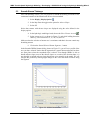
1
v. 10.0 WMS 10.0 Tutorial Spatial Hydrologic Modeling – Developing a GSSHA Model using the Hydrologic Modeling Wizard Learn how to setup a basic GSSHA model using the WMS interface Objectives Step through the hydrologic modeling wizard to build a basic GSSHA model. Run the model through the GSSHA analysis engine. Read the GSSHA results and view an animation of the results. Prerequisite Tutorials Watershed Modeling – DEM Delineation Required Components Data Drainage Map Hydrology 2D Grid GSSHA Page 1 of 17 Time 30-60 minutes © Aquaveo 2015 1 Contents 1 2 3 Contents ............................................................................................................................... 2 Introduction ......................................................................................................................... 2 Watershed Delineation using the Hydrologic Modeling Wizard .................................... 2 3.1 Project Filename ........................................................................................................... 2 3.2 Define Project Bounds ................................................................................................. 3 3.3 Watershed Data by Reading Files ................................................................................ 3 3.4 Compute Flow Directions and Accumulations ............................................................. 4 3.5 Choose Outlet Location ................................................................................................ 4 3.6 Delineate Watershed .................................................................................................... 5 4 Select Model ......................................................................................................................... 6 5 Define and Smooth Streams ............................................................................................... 6 5.1 Define Channel Geometry ............................................................................................ 6 5.2 Redistribute Vertices .................................................................................................... 7 5.3 Smooth Stream Thalwegs ............................................................................................. 8 6 Create 2D Grid .................................................................................................................... 9 7 Job Control .......................................................................................................................... 9 8 Define Land Use and Soil Data ........................................................................................ 10 9 Hydrologic Computations ................................................................................................ 10 9.1 Create Index Maps ..................................................................................................... 10 9.2 Define Model Parameters using Index Map Tables ................................................... 11 9.3 Additional Model Parameters ..................................................................................... 12 10 Define Precipitation .......................................................................................................... 12 11 Clean Up Model ................................................................................................................. 13 12 Run GSSHA ....................................................................................................................... 13 13 Post-processing and Visualization ................................................................................... 13 13.1 Outlet Hydrograph ..................................................................................................... 14 13.2 Summary File ............................................................................................................. 14 13.3 Grid Depth Contours .................................................................................................. 14 13.4 Stream Depth Contours .............................................................................................. 15 13.5 Creating an Animation Film Loop ............................................................................. 16 14 Conclusion.......................................................................................................................... 17 2 Introduction Gridded Surface Subsurface Hydrologic Analysis (GSSHA) is a physically based, distributed parameter, hydrologic model developed by the Engineering Research and Development Center of the Army Corps of Engineers. A detailed user’s manual and additional GSSHA tutorials can be found at www.gsshawiki.com. In this tutorial we will create a GSSHA model using data for Park City, UT and the Hydrologic Modeling Wizard. 3 Watershed Delineation using the Hydrologic Modeling Wizard 3.1 Project Filename 1. Close all instances of WMS Page 2 of 17 © Aquaveo 2015 WMS TutorialsSpatial Hydrologic Modeling – Developing a GSSHA Model using the Hydrologic Modeling Wizard 2. Open WMS 3. Click on the Hydrologic Modeling Wizard button at the bottom of the WMS window The Hydrologic Modeling Wizard will guide you through the modeling process. You can follow each step from the beginning or jump in and out at any step as needed. All of the WMS menus/tools work while the wizard is open. 4. Click on the Browse button to specify the path location and set a file name for the project 5. Locate the Hydrologic Models folder in the files for this tutorial. If needed, download the tutorial files from www.aquaveo.com. 6. Browse to folder spatial\WMS\ 7. For the File name enter “ParkCity.wms” and click Save 8. Click on the Save button in the Hydrologic Modeling Wizard 9. Click Next > to advance to the next step 3.2 Define Project Bounds 1. Under Project projection system, select Define… 2. Select the Global Projection option 3. In the Select Projection dialog set: Projection to UTM Zone to 12 (114°W - 108°W – Northern Hemisphere) Datum to NAD83 Planar Units to METERS 4. Select OK 5. Set the Vertical Projection to NAVD 88 (US) 6. Set the Vertical Units to Meters 7. Select OK 8. Click Next > to advance to the next step 3.3 Watershed Data by Reading Files 1. Click on the File | Open button 2. Locate the folder spatial\ RawData\ParkCity\ (all file folders referenced below are relative to this location) 3. In the \DEM\ file folder open “ned_35172081.hdr” 4. Select OK to import the NED GridFloat DEM WMS reads the projection data that comes with the DEM and converts the DEM projection to the project projection system specified in section 3.2. Page 3 of 17 © Aquaveo 2015 WMS TutorialsSpatial Hydrologic Modeling – Developing a GSSHA Model using the Hydrologic Modeling Wizard 5. Click on the File | Open button 6. In the \Luse\ file folder open “salt_lake_city.shp” 7. Click on the File | Open button 8. In the \SSURGO_Soil\Joinedsoil\ folder open “SSURGO_Soil.shp” 9. Turn off the display of all GIS Layers in the Project Explorer Now you should be able to see the DEM contours behind the modeling wizard in the WMS main window. 10. Click Next > to advance a few steps. Note that you have now read a DEM, Land use data, and soil data. These are the basic requirements of a GSSHA model. 3.4 Compute Flow Directions and Accumulations All GSSHA input files require metric units. WMS writes GSSHA input according to the model units rather than the computational units. This means that any of the options for computational units are valid because they are used for display purposes only. 1. Set the computational units for sub-basin areas to Square Miles 2. Set the computational units for distances to Feet 3. Select Compute TOPAZ TOPAZ uses the DEM data to compute flow directions and accumulations, which are used to infer the stream locations. 4. Click Close when TOPAZ terminates 5. Set the Min flow accumulation threshold to 0.2 mi^2 6. Click on the Apply to Display button 7. Click Next > to advance to the next step 3.5 Choose Outlet Location 1. Choose the Create Outlet Point tool in the Hydrologic Modeling Wizard 2. Click on the outlet location in the WMS graphics window using Figure 3-1 as a guide (you can use the middle scroll button of mouse to zoom in or out) 3. Click Next > to advance to the next step Page 4 of 17 © Aquaveo 2015 WMS TutorialsSpatial Hydrologic Modeling – Developing a GSSHA Model using the Hydrologic Modeling Wizard Figure 3-1: DEM Contours and Streams delineated from DEM 3.6 Delineate Watershed 1. Click on the Delineate Watershed button Your watershed will look somewhat like Figure 3-2 Figure 3-2: Delineated Watershed Page 5 of 17 © Aquaveo 2015 WMS TutorialsSpatial Hydrologic Modeling – Developing a GSSHA Model using the Hydrologic Modeling Wizard 2. Save your WMS project by selecting File | Save in the main WMS window 3. Click Next > to advance to the next step 4 Select Model 1. Set the model to be GSSHA 2. Click on the Initialize Model Data button 3. Click Next > to advance to the next step 5 Define and Smooth Streams All the streams defined so far in GSSHA are generic and they do not have any defined shape or geometry. Also, because of anomalies in the DEM elevations, some stream bed elevations will not decrease between upstream and downstream cells when the 2D grid is created. This “stream smoothing” problem creates issues when running a GSSHA simulation. In this step, we will define the channel cross section and roughness properties and we will also check and smooth the channel bottom. After you define the channel data and smooth streams, WMS assigns the smoothed stream elevations to the 2D grid wherever streams intersect 2D grid cells. This prevents you from having adverse slopes between grid cells on the 2D grid. 5.1 Define Channel Geometry For this example, we will assume that all the stream segments have the same cross section. You may enter different cross sections for individual stream arcs by selecting them and following the same procedure outlined in this section. 1. Select Display | Display Options 2. In the DEM Data tab toggle off the options for Stream and Flow Accumulation 3. Select OK 4. Turn off the display of the DEM ned_35172081 (Converted) in the Project Explorer 5. In the hydrologic modeling wizard, choose the Select feature line branch tool 6. Click on stream segment #1 as shown in Figure 5-1 (you may need to use the scroll bar on the mouse to zoom in) 7. Click on the Set Selected Arc Attributes… button 8. In the yellow All row of the spreadsheet: Change the Type to Trapezoidal channel Page 6 of 17 © Aquaveo 2015 WMS TutorialsSpatial Hydrologic Modeling – Developing a GSSHA Model using the Hydrologic Modeling Wizard For Manning’s n enter 0.025 For Depth (m) enter 1.0 For Bottom width (m) enter 3.0 For Side slope (H:V) enter 1.45 1. Select OK Figure 5-1: GSSHA stream segments 5.2 Redistribute Vertices Before smoothing the streams, it is a good idea to redistribute the vertices on the streams because GSSHA requires a constant computational length between vertices along the 1-D streams. Also, we will make the spacing similar to the grid resolution. 1. Click on the Redistribute Vertices on All Streams… button 2. For Spacing enter 90.0 3. Toggle on the option to Use Cubic Spline 4. Select OK Page 7 of 17 © Aquaveo 2015 WMS TutorialsSpatial Hydrologic Modeling – Developing a GSSHA Model using the Hydrologic Modeling Wizard 5.3 Smooth Stream Thalwegs After redistributing vertices, you will proceed to smooth the thalweg elevations of the continuous branches of the channel until all have been smoothed. 1. Select Display | Display Options 2. In the Map Data tab toggle on the option for Adverse Slopes 3. Select OK Notice that streams with adverse slopes are displayed using the color defined in the display options. 4. In the hydrologic modeling wizard, choose the Select Feature Arc tool . 5. Select stream arc #1 as shown in Figure 5-1 and while holding down the shift key, select stream arcs #3, #7, #9, #14, and #15. Make sure that the selection of stream arcs is continuous and that it does not contain any branching streams. 6. Click on the Smooth Selected Stream Segments… button. In the Smooth GSSHA Streams dialog, shown in Figure 5-2, you will see a profile of the arcs you have selected. Notice that the segment has a general downward trend, but there are some places where the streambed slope is adverse. Even though GSSHA is able to handle adverse slopes, most of the adverse slopes are a result of the elevation data; it is not desirable to include adverse slopes that do not exist naturally in the model. We will mitigate this problem by making slight changes to the vertex and node elevations along the segment. Figure 5-2: GSSHA Stream Editor Page 8 of 17 © Aquaveo 2015 WMS TutorialsSpatial Hydrologic Modeling – Developing a GSSHA Model using the Hydrologic Modeling Wizard 7. Click the Interpolate Stream Elevations button as many times as needed to generate a smooth stream segment with no uphill flow. 8. Select OK. If uphill flow cannot be eliminated in this manner, you can edit individual points by selecting a point on the plot (hover directly over the point on the plot and move it up or down), then dragging the point to a new position or editing the Stream elevation value. Be especially careful to make sure the nodes next to the outlet are not adverse. You can zoom into individual points by clicking and dragging a box around section of the plot. It is also possible to pan in any direction by moving the scroll bars along the sides of the plot. Right-clicking on the plot will give you a menu with several choices, including options to output data from the plot, set display options, and frame the plot to its maximum extents. Once the stream segment you have selected is smooth, select a new stream segment with an adverse slope or combination of segments to smooth. Repeat the smoothing process outlined in steps 4 through 8 until there are no stream segments with an adverse slope. Your streams are now ready for use in the GSSHA model. 9. After you have finished correcting the inverse slopes on your streams by smoothing all your stream segments, click Next > to advance to the next step. 6 Create 2D Grid Now that you have smoothed your streams, you are ready to create a 2D grid. When you create the grid, WMS assigns the smoothed stream elevations to the 2D grid wherever streams intersect 2D grid cells. 1. Make sure that the Enter cell size option is selected. 2. For the X-dimension enter a cell size of 90 meters (the Y-dimension is automatically set to the same value as the X-dimension). 3. Click on the Create 2D Grid button. 4. Select OK to interpolate elevations for each grid cell from the background DEM (Make sure Interpolate GSSHA Coverage Streams is selected). 5. Click Yes to delete the existing background DEM. 6. Click Next > to advance to the next step. 7 Job Control 1. Set the Starting date to 01/01/2008 2. Set the Starting time to 12:00:00 PM 3. Set the Ending date to 01/03/2008 4. Set the Ending time to 12:00:00 PM 5. Set the Time interval to 10 sec 6. Click on the Set Job Control Data button Page 9 of 17 © Aquaveo 2015 WMS TutorialsSpatial Hydrologic Modeling – Developing a GSSHA Model using the Hydrologic Modeling Wizard 7. Click Next > to advance to the next step 8 Define Land Use and Soil Data Since you have already read land use and soil shapefiles, you are ready to convert these to feature data in the map module, which will be used to develop hydrologic input parameters. 1. Verify that “salt_lake_city.shp” is set to a Land Use shapefile type. 2. Make sure that “SSURGO_Soil.shp” is set to a Soil Type shapefile type. 3. Click on the Create Coverages… button. 4. Select Next > in the GIS to Feature Objects Wizard. Notice that WMS automatically set the LUCODE in the shapefile to be mapped to the Land use parameter in WMS. 5. Select Next > 6. Select Finish 7. Repeat the same mapping process for the soil shapefile WMS automatically maps HYDGRP to SCS soil type, TEXTURE to Texture, KSAT to Hydraulic conductivity, MOISTURE to Initial moisture, FIELDCAP to Field capacity, and WILTINGPT to Wilting point. 8. Click Next > in the Hydrologic Modeling Wizard to advance to the next step 9 Hydrologic Computations 9.1 Create Index Maps 1. Click on the Compute Index Mapping Tables… button 2. For Input coverage (1) choose Land Use and set the Coverage attribute to Id 3. Enter an Index map name of “Land Use” 4. Click on the Coverages -> Index Map button 5. For Input coverage (1) choose Soil Type and set the Coverage attribute to Texture 6. Enter an Index map name of “Soil Type” 7. Click on the Coverages -> Index Map button 8. Toggle on the Input coverage (2) option so that you can create a combined index map based on both land use and soil type coverages 9. For Input coverage (2) choose Land Use and set the Coverage attribute to Id Page 10 of 17 © Aquaveo 2015 WMS TutorialsSpatial Hydrologic Modeling – Developing a GSSHA Model using the Hydrologic Modeling Wizard 10. Enter an Index map name of “Combined” 11. Click on the Coverages -> Index Map button 12. Select Done in the GSSHA Maps dialog You should see three index maps on the data tree under the 2D Grid Data. The GSSHA Map Table Editor dialog will automatically appear. You will now need to define the index mapping parameters. 9.2 Define Model Parameters using Index Map Tables 1. Switch to the Roughness tab (it is usually selected by default). 2. For the Using index map field select Land Use. 3. Click on the Generate IDs button. IDs for each of the land use type polygons that overlay the 2D grid are generated and displayed. 4. Now switch to the Infiltration tab. 5. Select Yes to turn the infiltration option on. 6. In the Job Control Dialog, select the Green & Ampt with soil moisture redistribution option. 7. Select OK. 8. For the Using index map field select Combined. 9. Click the Generate IDs button. This will generate a unique ID for all possible combinations of land use and soil type data within the watershed. 10. Switch to the Initial Moisture tab. 11. For the Using index map field select Soil Type. 12. Click on the Generate IDs button. 13. Click on the Import table… button at the bottom part of the GSSHA Map Table Editor. 14. Browse to the spatial folder. 15. Open the file gssha.cmt NOTE: This table has typical values for the watershed parameters based on standard soil type and land use classification. Importing this table will populate model input parameters with the values in the file. Model input parameters should always be verified. One important thing to remember is that the values from the table are not absolute and the modeler needs to take ownership of them and adjust as necessary for the specific conditions of a given area. Generally these values are best estimated either by field measurement or by model calibration. Values obtained from this table should only be used as an initial estimate of the corresponding parameters. 16. Switch back to the Roughness tab. Page 11 of 17 © Aquaveo 2015 WMS TutorialsSpatial Hydrologic Modeling – Developing a GSSHA Model using the Hydrologic Modeling Wizard Notice the preliminary values for roughness that were entered based on the land use data. Enter a suitable number for any entry with a zero value. 17. Switch to the Infiltration tab. The values listed in this spreadsheet are based on soil texture only. Notice that the index map contains a land use and soil type for each index map ID. One would expect the infiltration values for sand in an agricultural area to be different from the infiltration value for sand in a residential area. Similarly, loam in a forest environment will have different infiltration values than loam in an industrial area. Based on your knowledge of how land use affects infiltration properties of the soil, make suitable adjustments to the default parameters. 18. Look at the land use IDs and adjust Hydraulic conductivity, Capillary head, porosity etc. as necessary. 19. Switch to the Initial Moisture tab. 20. If you want to adjust the values for initial moisture, enter these values here (make sure that the values you enter here are smaller than the values for porosity in the Infiltration tab). 21. Select Done in the GSSHA Map Table Editor dialog. 9.3 Additional Model Parameters 1. Click on the Edit Parameters… button on the modeling wizard to open the GSSHA Job Control Parameters dialog. 2. For Channel routing computation scheme choose Diffusive Wave. 3. Click on the Output Control button. 4. Under the Gridded data sets data, toggle on the Cumulative infiltration depth and Infiltration rate options. 5. Under Link / Node data sets toggle on the Channel Depth and Channel flow options. 6. Change the Write frequency of these datasets to 15 min. 7. Change the Hydrograph Write frequency to 5 minutes. 8. Set the Hydrograph Output units to be English (all computations in GSSHA are performed using metric units, but the outlet hydrograph will be automatically converted from m3/s to cfs). 9. Select OK to close the GSSHA Output Control dialog. 10. Select OK to close the GSSHA Job Control Parameters dialog. 11. Click Next > in the Hydrologic Modeling Wizard to advance to the next step. 10 Define Precipitation 1. Click on the Define Precipitation… button. 2. For Rainfall event(s) select Hyetograph. Page 12 of 17 © Aquaveo 2015 WMS TutorialsSpatial Hydrologic Modeling – Developing a GSSHA Model using the Hydrologic Modeling Wizard 3. Click on the Define Distribution… button. 4. In the XY Series Editor change the Selected Curve to typeI-24hour. This is the temporal distribution of an SCS Type I - 24 hour storm. 5. Select OK. 6. Enter an Average Depth of 63.5 mm. 7. Select OK. 8. Click Next > to advance to the next step. 11 Clean Up Model You are done defining most of the parameters and components required for the model. 1. Click on the Clean Up Model button. 2. Select OK. 3. Click Done to close the model checker. 4. Click Close when CleanDam is finished running in the Model Wrapper. 5. Click on the Save button to save the GSSHA project file. 6. Browse to the spatial\GSSHA\ directory. 7. Enter “ParkCity.prj” and select Save. 8. Select Close to close the Hydrologic Modeling Wizard. 12 Run GSSHA 1. In the 2D Grid module select GSSHA | Run GSSHA 2. Toggle off the Suppress screen printing option 3. Select OK The discharge at each time step is displayed in the model wrapper. 4. Click Close when the simulation is complete and WMS will read in the solution files 13 Post-processing and Visualization This section of the tutorial describes different methods of viewing and visualizing GSSHA model results. GSSHA outputs multiple solution files including an outlet hydrograph file, a summary file, and solution data sets, which appear in two separate folders in the WMS Project Explorer. All 2D grid data sets are displayed in the Solution folder that is part of the GSSHA model in the 2D Grid Data section of the Project Explorer. The link/node data sets that GSSHA outputs when channel routing occurs appear in a different Solution folder in the 2D Scatter Data section of the Project Explorer. Page 13 of 17 © Aquaveo 2015 WMS TutorialsSpatial Hydrologic Modeling – Developing a GSSHA Model using the Hydrologic Modeling Wizard 13.1 Outlet Hydrograph 1. Choose the Select hydrographs tool. 2. Double click on the hydrograph icon that is displayed next to the outlet grid cell. This opens the runoff hydrograph in a plot window. If desired, you can export the time series data for the hydrograph by right-clicking on the hydrograph plot window and selecting Export/Print…. 3. Close the hydrograph plot window by clicking on the X in the upper right corner of the window. 4. Select Display | Display Options… . 5. In the 2D Grid tab toggle OFF the display of everything except Cells and Contours. 6. In the Hydrologic Modeling tab toggle OFF the display of Hydrograph Icons. 7. Select OK. 13.2 Summary File 1. In the 2D Grid Data folder of the Project Explorer expand the ParkCity GSSHA model folder, if necessary. 2. Expand the Solution folder under the ParkCity GSSHA model, if necessary. 3. Double-click on the Summary File in the Solution folder. 4. If prompted to select an editor, click OK. Look through the summary file. It is good to check things like the mass balance and the volume remaining on the surface to know that GSSHA is simulating the processes correctly. 5. Close the summary file when you are done viewing it. 13.3 Grid Depth Contours 1. Toggle OFF the Coverages folder in the Project Explorer. 2. Right-click on the “depth” data set in the Solution folder in the Project Explorer and select Contour Options…. 3. Change the Contour Method to Color Fill. 4. Click on the Legend… button. 5. Toggle on the option to Display legend. 6. Select OK. 7. Select OK. 8. Click on the first time step shown in the Properties window. Page 14 of 17 © Aquaveo 2015 WMS TutorialsSpatial Hydrologic Modeling – Developing a GSSHA Model using the Hydrologic Modeling Wizard Use the down arrow key (on the keyboard) to cycle through the time steps and view the overland flow depth. In this particular model overland flow depth values first become evident approximately 10 hours after the start of the simulation at 10:00 am on 01/01/2008. Skip ahead to this time step to view depth values. 13.4 Stream Depth Contours 1. Select the Stream depth data set in the ParkCity (GSSHA) solution folder under the 2D Scatter Data folder in the Project Explorer 2. Select Display | Display Options 3. In the general options, turn off Auto z-mag and set the Z-magnification to 1.0. 4. In the Scatter Point tab toggle OFF the Symbols option and toggle ON the Contours option 5. Change the Radius to 30 6. Set the Z magnification to 100 (this only applies to the link/node stream depth contours) 7. Select OK 8. Use the Rotate tool to position the grid so that it appears similar to Figure 13-1 Figure 13-1: Rotated watershed 9. Click on the first time step shown in the Properties window Use the down arrow key (on the keyboard) to cycle through the time steps and view the channel flow depth. In this particular model channel flow depth values first become evident approximately 10 hours after the start of the simulation at 10:00 am on 01/01/2008. Skip ahead to this time step to view depth values. Notice the changing bar diagrams. These bars represent the flood wave magnitude along the stream at each time step. Page 15 of 17 © Aquaveo 2015 WMS TutorialsSpatial Hydrologic Modeling – Developing a GSSHA Model using the Hydrologic Modeling Wizard Figure 13-2 shows the overland flow depth contours changing simultaneously with the flood wave bar diagrams. This gives a clearer idea of the natural process of overland flow. Figure 13-2: Grid and Stream Depth Contours 13.5 Creating an Animation Film Loop These processes can also be visualized in a film loop. WMS creates two types of file loops. One type is the standard .avi (movie) file and the other type can be viewed in Google Earth so that the flood animation is displayed over a Google Earth image. 1. Select Display | View | Plan View . 2. Right-click on the “depth” data set in the Solution folder of the Project Explorer and select Contour Options…. 3. Change the Contour Method to Normal Linear. 4. Select OK. 5. In the 2D Grid module select Data | Film Loop…. 6. Choose the Create New Filmloop option. 7. For Type select the Scalar/Vector Animation option and click Next >. 8. Toggle on the Scalar Data Set option. 9. Change the simulation run time to run from 9:00 PM to 11:30 PM. 10. For Number of Frames enter 30. 11. Click Next >. 12. Click Finish (do not change the clock options). WMS will take some time to create the film loop. It will automatically begin playing once it is completely saved. If Google Earth is installed, Google Earth will start and the Page 16 of 17 © Aquaveo 2015 WMS TutorialsSpatial Hydrologic Modeling – Developing a GSSHA Model using the Hydrologic Modeling Wizard movie will appear in the correct geographic location. If Google Earth is not installed, the AVI file will run in a movie player. If the data seems somewhat jumpy while scrolling through the time steps (or making a movie) this is because output time step is too large. 14 Conclusion In this exercise you learned how to set up a basic GSSHA model, including channel routing, using the Hydrologic Modeling Wizard. The wizard guides you through the processes of delineating a watershed, creating a 2D grid, entering GSSHA job control data, defining and smoothing streams, and developing hydrologic input parameters. Options for post-processing GSSHA model results were also introduced. Page 17 of 17 © Aquaveo 2015