Download OFGT User Manual

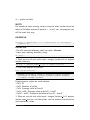
Open Foris Geospatial Toolkit
USER MANUAL
Food and Agriculture Organization of the United Nations
Viale delle Terme di Caracalla, 00153 Rome, Italy
Version 1.25.4 October 2013
Contents
1 Introduction
1.1 About this manual . . . . . .
1.2 What is OFGT? . . . . . . .
1.3 The great potential of OFGT
1.4 First time users . . . . . . .
.
.
.
.
.
.
.
.
.
.
.
.
.
.
.
.
.
.
.
.
.
.
.
.
.
.
.
.
.
.
.
.
.
.
.
.
.
.
.
.
.
.
.
.
.
.
.
.
.
.
.
.
.
.
.
.
.
.
.
.
.
.
.
.
.
.
.
.
.
.
.
.
.
.
.
.
5
5
5
6
6
2 License
6
3 Installation of Open Foris Geospatial Toolkit
3.1 Linux: debian-based distributions (Ubuntu, Debian, etc.) . . .
3.2 Linux: rpm-based systems (PCLinuxOS, RedHat, SuSE, etc.)
3.3 Mac OS-X: Lion . . . . . . . . . . . . . . . . . . . . . . . .
3.4 Windows Cygwin installation . . . . . . . . . . . . . . . . . .
7
7
7
8
9
.
.
.
.
.
.
.
.
4 Get Info
11
5 Update the tools
11
6 Uninstallation
11
7 OFGT- Tools documented
12
General Tools
7.1 CsvToPolygon.py . . . . . . . . . . . . . .
7.2 genericCsvToPolygon.py . . . . . . . . . .
7.3 genericGEkml2csv.bash . . . . . . . . . .
7.4 GExml2csv.bash . . . . . . . . . . . . . .
7.5 oft-addattr.py . . . . . . . . . . . . . . .
7.6 oft-addpct.py . . . . . . . . . . . . . . . .
7.7 oft-admin-mask.bash . . . . . . . . . . . .
7.8 oft-bb . . . . . . . . . . . . . . . . . . .
7.9 oft-classvalues-compare.bash - To be tested
7.10 oft-classvalues-plot.bash - To be tested . .
7.11 oft-combine-masks.bash . . . . . . . . . .
7.12 oft-compare-overlap.bash - To be tested .
7.13 oft-crop.bash . . . . . . . . . . . . . . . .
7.14 oft-cuttile.pl . . . . . . . . . . . . . . . .
7.15 oft-filter . . . . . . . . . . . . . . . . . .
7.16 oft-gengrid.bash . . . . . . . . . . . . . .
7.17 oft-getcorners.bash . . . . . . . . . . . . .
12
12
14
17
19
20
23
26
28
30
33
36
41
45
47
51
54
56
User Manual
.
.
.
.
.
.
.
.
.
.
.
.
.
.
.
.
.
.
.
.
.
.
.
.
.
.
.
.
.
.
.
.
.
.
.
.
.
.
.
.
.
.
.
.
.
.
.
.
.
.
.
.
.
.
.
.
.
.
.
.
.
.
.
.
.
.
.
.
.
.
.
.
.
.
.
.
.
.
.
.
.
.
.
.
.
.
.
.
.
.
.
.
.
.
.
.
.
.
.
.
.
.
.
.
.
.
.
.
.
.
.
.
.
.
.
.
.
.
.
.
.
.
.
.
.
.
.
.
.
.
.
.
.
.
.
.
.
.
.
.
.
.
.
.
.
.
.
.
.
.
.
.
.
.
.
.
.
.
.
.
.
.
.
.
.
.
.
.
.
.
.
.
.
.
.
.
.
.
.
.
.
.
.
.
.
.
.
.
.
.
.
.
.
.
.
.
.
.
.
.
.
.
.
.
2
7.18
7.19
7.20
7.21
7.22
oft-polygonize.bash . . . . .
oft-sample-within-polys.bash
oft-shptif.bash . . . . . . .
oft-sigshp.bash . . . . . . .
PointsToSquares.py . . . .
.
.
.
.
.
.
.
.
.
.
.
.
.
.
.
.
.
.
.
.
.
.
.
.
.
.
.
.
.
.
.
.
.
.
.
.
.
.
.
.
.
.
.
.
.
.
.
.
.
.
.
.
.
.
.
.
.
.
.
.
.
.
.
.
.
.
.
.
.
.
.
.
.
.
.
.
.
.
.
.
.
.
.
.
.
.
.
.
.
.
.
.
.
.
.
.
.
.
.
.
58
60
63
65
69
Image Manipulation
7.23 multifillerThermal.bash . . . . . .
7.24 oft-calc . . . . . . . . . . . . . .
7.25 oft-chdet.bash . . . . . . . . . .
7.26 oft-clip.pl . . . . . . . . . . . . .
7.27 oft-combine-images.bash . . . . .
7.28 oft-gapfill . . . . . . . . . . . . .
7.29 oft-ndvi.bash . . . . . . . . . . .
7.30 oft-prepare-images-for-gapfill.bash
7.31 oft-reclass . . . . . . . . . . . .
7.32 oft-shrink . . . . . . . . . . . . .
7.33 oft-stack . . . . . . . . . . . . .
7.34 oft-trim . . . . . . . . . . . . . .
7.35 oft-trim-maks.bash . . . . . . . .
.
.
.
.
.
.
.
.
.
.
.
.
.
.
.
.
.
.
.
.
.
.
.
.
.
.
.
.
.
.
.
.
.
.
.
.
.
.
.
.
.
.
.
.
.
.
.
.
.
.
.
.
.
.
.
.
.
.
.
.
.
.
.
.
.
.
.
.
.
.
.
.
.
.
.
.
.
.
.
.
.
.
.
.
.
.
.
.
.
.
.
.
.
.
.
.
.
.
.
.
.
.
.
.
.
.
.
.
.
.
.
.
.
.
.
.
.
.
.
.
.
.
.
.
.
.
.
.
.
.
.
.
.
.
.
.
.
.
.
.
.
.
.
.
.
.
.
.
.
.
.
.
.
.
.
.
.
.
.
.
.
.
.
.
.
.
.
.
.
.
.
.
.
.
.
.
.
.
.
.
.
.
.
.
.
.
.
.
.
.
.
.
.
.
.
.
.
.
.
.
.
.
.
.
.
.
.
.
.
.
.
.
.
.
.
.
.
.
.
.
.
70
71
72
78
80
81
83
88
91
94
99
99
101
103
Statistics
7.36 oft-ascstat.awk .
7.37 oft-avg . . . . .
7.38 oft-countpix.pl .
7.39 oft-crossvalidate
7.40 oft-extr . . . . .
7.41 oft-his . . . . .
7.42 oft-mm . . . . .
7.43 oft-segstat . . .
7.44 oft-stat . . . . .
.
.
.
.
.
.
.
.
.
.
.
.
.
.
.
.
.
.
.
.
.
.
.
.
.
.
.
.
.
.
.
.
.
.
.
.
.
.
.
.
.
.
.
.
.
.
.
.
.
.
.
.
.
.
.
.
.
.
.
.
.
.
.
.
.
.
.
.
.
.
.
.
.
.
.
.
.
.
.
.
.
.
.
.
.
.
.
.
.
.
.
.
.
.
.
.
.
.
.
.
.
.
.
.
.
.
.
.
.
.
.
.
.
.
.
.
.
.
.
.
.
.
.
.
.
.
.
.
.
.
.
.
.
.
.
.
.
.
.
.
.
.
.
.
.
.
.
.
.
.
.
.
.
.
.
.
.
.
.
.
.
.
.
.
.
.
.
.
.
.
.
.
.
.
.
.
.
.
.
.
105
106
108
111
113
117
121
127
129
134
Classification
7.45 oft-cluster.bash . . . . . . . .
7.46 oft-kmeans . . . . . . . . . .
7.47 oft-nn - To be tested . . . . .
7.48 oft-nn-training-data.bash . . .
7.49 oft-normalize.bash . . . . . .
7.50 oft-prepare-image-for-nn.bash
7.51 oft-unique-mask-for-nn.bash .
.
.
.
.
.
.
.
.
.
.
.
.
.
.
.
.
.
.
.
.
.
.
.
.
.
.
.
.
.
.
.
.
.
.
.
.
.
.
.
.
.
.
.
.
.
.
.
.
.
.
.
.
.
.
.
.
.
.
.
.
.
.
.
.
.
.
.
.
.
.
.
.
.
.
.
.
.
.
.
.
.
.
.
.
.
.
.
.
.
.
.
.
.
.
.
.
.
.
.
.
.
.
.
.
.
.
.
.
.
.
.
.
.
.
.
.
.
.
.
.
.
.
.
.
.
.
.
.
.
.
.
.
.
137
138
142
146
151
154
156
158
User Manual
.
.
.
.
.
.
.
.
.
.
.
.
.
.
.
.
.
.
.
.
.
.
.
.
.
.
.
.
.
.
.
.
.
.
.
.
.
.
.
.
.
.
.
.
.
.
.
.
.
.
.
.
.
.
3
Segmentation
160
7.52 oft-clump . . . . . . . . . . . . . . . . . . . . . . . . . . . . . . 161
7.53 oft-seg . . . . . . . . . . . . . . . . . . . . . . . . . . . . . . . 163
Projection
166
7.54 oft-getproj.bash . . . . . . . . . . . . . . . . . . . . . . . . . . 167
User Manual
4
1
Introduction
1.1
About this manual
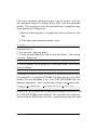
The user manual is developed to help getting into spatial analysis using the Open
Foris Geopsatial Toolkit. It gives basic explanations of how OFGT functions. It is
not attempted to explain the theoretical background on how to do geo-spatial
analysis using remote sensing or GIS, but rather will guide you through hands-on
examples for each tool, next to some general areas, such as the installation.
Further, the manual will link to relevant man pages and other documentation.
In addition, the user manual is written in a way that it can be understood by people who are experienced Windows or Mac users, but have not
used Linux or OFGT much before. Sources and documentation for OFGT
can be obtained here: http://km.fao.org/OFwiki/index.php/Open_Foris_
Geospatial_Toolkit
1.2
What is OFGT?
OFGT - Open Foris Geospatial Toolkit is a a collection of prototype commandline utilities for processing of geographical data. The tools can be divided into
stand-alone programs and scripts and they have been tested mainly in Ubuntu
Linux environment although can be used with other linux distros, Mac OS, and
MS Windows (Cywgin) as well. Most of the stand-alone programs use GDAL
libraries and many of the scripts rely heavily on GDAL command-line utilities.
The OFGT project started under the Open Foris Initiative to develop, share
and support software tools and methods for multi-purpose forest assessment,
monitoring and reporting. The Initiative develops and supports innovative, easyto-use tools needed to produce reliable, timely information on the state of forest
resources and their uses. The command-line tools aim to simplify the complex
process of transforming raw satellite imagery for automatic image processing to
produce valuable information. These tools contain radiometric harmonisation,
image segmentation and image arithmetic, as well as image statistics, feature
extraction and other image processing analysis.
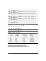
Overview of OFGT versions currently available
• OFGT 1.25.4 - continuously updated
• OFGT 1.0 -
User Manual
5
1.3
The great potential of OFGT
The toolkit comes to its own when dealing with large data sets:
• First of all the processing itself takes a fraction of time than with
conventional software.
• And second, automatised data processing makes applications repeatable, which is of high advantage for many projects.
• All tools and methods developed under the Initiative are open-source.
1.4
First time users
First time users, the terminal is your friend: The Open Foris Geospatial Toolkit
tutorial is aiming to provide straight forward guidelines and examples to help first
time users to familiarise themselves with the Open Foris Geospatial Toolkit. This
includes the installation of Ubuntu, various geospatial tools and, in particular,
the installation and application of the Open Foris Geospatial Toolkit. You do not
need to be an expert, we just would like you to be curious to try things out. Do
not be afraid of using the command-line! We know that the terminal window is
for many users a barrier of being afraid ruining everything and having to start
from scratch. These days the terminal is not exclusively for advanced computer
enthusiasts. Give it a try and just start playing around following the tutorials and
instructions you can find in the wiki.
2
License
Open Foris Geospatial Toolkit is released under GNU GPLv3 license.
User Manual
6
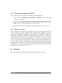
3
Installation of Open Foris Geospatial Toolkit
The Open Foris Geospatial Toolkit comes with an installer which is frequently
updated. It is named OpenForisToolkit.run. To run the installer please use the
Terminal.
3.1
Linux: debian-based distributions (Ubuntu, Debian,
etc.)
The installer has been tested with various Ubuntu Linux versions and it should
work with other Debian based distros as well.
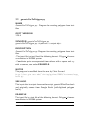
1. First make sure that you have installed all the necessary gdal and gsl libraries
and tools. If you do not have them download and install them by using
following commands:
sudo
sudo
sudo
sudo
sudo
sudo
sudo
sudo
sudo
sudo
sudo
apt−g e t
apt−g e t
apt−g e t
apt−g e t
apt−g e t
apt−g e t
apt−g e t
apt−g e t
apt−g e t
apt−g e t
apt−g e t
install
install
install
install
install
install
install
install
install
install
install
gcc
g++
g d a l −b i n
l i b g d a l 1 −dev
l i b g s l 0 −dev
libgsl0ldbl
python−g d a l
python−g d a l
perl
python−s c i p y
python−t k
2. Then download the OpenForisToolkit.run installer
wget h t t p : // f o r i s . f a o . o r g / s t a t i c / g e o s p a t i a l t o o l k i t / r e l e a s e s /
Op en Fori sTool k i t . run
sudo chmod u+x O p e n F o r i s T o o l k i t . r u n
sudo . / O p e n F o r i s T o o l k i t . r u n
3. To accept the license terms type 1 and hit enter.
3.2
Linux: rpm-based systems (PCLinuxOS, RedHat, SuSE,
etc.)
Open Foris Toolkit is tested on and we recommend PCLinuxOS. Always ensure
that your system is fully updated: Open Synaptic, click Reload to get a current
file list, click Mark All Upgrades, click Apply.
User Manual
7
1. If you do not have gdal and gsl libraries and tools installed, install them via
Synaptic:
• Open Synaptic, click Reload, click Search, then search for the following
packages and and mark them for installation: libgdal-devel, gdal, gdalpython, prom, gsl-devel, gsl-progs
• Click Apply to install them
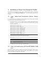
2. Download the OpenForisToolkit.run installer
wget h t t p : // f o r i s . f a o . o r g / s t a t i c / g e o s p a t i a l t o o l k i t / r e l e a s e s /
Op en Fori sTool k i t . run
Make the installer executable open a Terminal and enter the command:
chmod u+x O p e n F o r i s T o o l k i t . r u n
Install OpenForisToolkit, enter the command:
s u −c ’ . / O p e n F o r i s T o o l k i t . r u n ’
3.3
Mac OS-X: Lion
1. Download wget, make it executable, and copy it into the system: open a
Terminal and enter the command:
chmod a+x wget ; sudo cp wget / u s r / b i n /
2. Download and install the latest version of the gsl-framework and gdalcomplete from kyngchaos:
3. Download the OpenForisToolkit.run installer
wget h t t p : // f o r i s . f a o . o r g / s t a t i c / g e o s p a t i a l t o o l k i t / r e l e a s e s /
Op en Fori sTool k i t . run
4. Making the installer executable open a Terminal and enter the command:
chmod u+x O p e n F o r i s T o o l k i t . r u n
5. Amend the $PATH environment for the installation, enter the command:
E x p o r t PATH=/ L i b r a r y / Frameworks /GSL . f r a m e w o r k / Programs : $PATH
6. Install OpenForisToolkit, enter the command:
sudo . / O p e n F o r i s T o o l k i t . r u n
User Manual
8
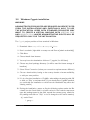
3.4
Windows Cygwin installation
WARNING
ADMINISTRATIVE PRIVILEGES ARE REQUIRED IN ORDER TO PERFORM THE INSTALLATIONS AND EVENTUALLY ALSO TO USE
THE APPLICATION. USERS WITH STANDARD PRIVILEGES MAY
WANT TO CREATE A VIRTUAL MACHINE WITH VIRTUAL BOX
AND UBUNTU 12.04 WHERE ADMINISTRATIVE RIGHTS WILL BE
REQUESTED ONLY FOR THE INSTALLATION.
The Cygwin project provides a Linux terminal in Windows.
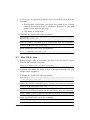
1. Download either setup-x86.exe or setup-x86 64.exe
2. Run it as admin (right-click on setup.exe and Run as [admin credentials])
3. Click Next
4. Choose Install from Internet
5. You may leave the destination folder as C:\cygwin (for All Users)
6. Choose any local package directory (it will be used for future storage of
installers)
7. Select Direct Connection (unless your connection requirements are different)
8. Choose a download site, basing on site country domain or known availability,
or add your own preferite
9. If it is a first time installation of CygWin, acknowledge the warning with OK
or click on ’Skip’ to activate them (if you already have CygWin installed,
you could skip the installation or check how the installation may affect the
existing version)
10. During the installation, ensure to flag the following options under the Bin
column (use the Search field for a faster retrieval of the needed components:
type the package name in the field, expand the correct group, search for
the package and click on ”Skip” to see it changed to the version number)
(a) under Devel
i. gcc-g++
User Manual
9
ii. make
(b) under Net
i. wget
(c) under Libs
i.
ii.
iii.
iv.
gsl
gsl-apps
gsl-devel
gsl-doc
11. Click Next
12. Flag ”Select required packages” and click Next to resolve the related
dependencies
13. Click Next
14. The installation may take some time
15. Choose whether or not to create a Desktop and a Start Menu icon
16. Click Finish
To compile the Open Foris Geospatial Toolkit you need to compile GDAL manually.
1. Download the installer from the gdal official repository (e.g. gdal-1.10.1.tar.gz)
2. Save it in your CygWin home folder (e.g. C:\cygwin\home or C:\cygwin64\home)
or in another destination of your choice
3. Run CygWin (NOTE: FOR INSTALLATION, RUN CYGWIN AS
ADMIN; Right click on Start >(All) Programs >CygWin >CygWin
Terminal and Run as [admin credentials])
4. Install GDAL using the following commands (the last two can take some
time to complete)
cd [ f o l d e r c o n t a i n i n g g d a l − 1 . 1 0 . 1 . t a r . gz ] ( e . g . cd C : / c y g w i n /
home , mind t h e s i m p l e s l a s h )
t a r −x v z f g d a l − 1 . 1 0 . 1 . t a r . gz
cd g d a l − 1 . 1 0 . 1
./ configure
make
make i n s t a l l
User Manual
10
Now you can install OpenForis. Still in CygWin, run the following commands:
wget h t t p : // f o r i s . f a o . o r g / s t a t i c / g e o s p a t i a l t o o l k i t / r e l e a s e s /
Op en Fori sTool k i t . run
chmod u+x O p e n F o r i s T o o l k i t . r u n
. / Op en Fori sTool k i t . run
4
Get Info
After the first installation, you can check the current version info with the
command:
sudo o f t −i n f o . b a s h
5
Update the tools
Update to the latest version use follwoing command:
sudo o f t −u p d a t e . b a s h
6
Uninstallation
You can also uninstall all the tools. To do that, enter the command:
sudo o f t − u n i n s t a l l . b a s h
User Manual
11
7
OFGT- Tools documented
GENERAL TOOLS
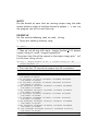
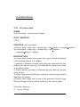
7.1
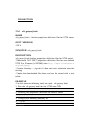
CsvToPolygon.py
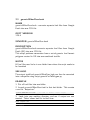
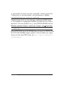
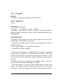
NAME
CsvToPolygon.py - converts CSV file from GExml2csv.bash into a
shapefile
OFGT VERSION
1.25.4
SYNOPSIS CsvToPolygon.py
CsvToPolygon.py <input.csv><output.shp>
DESCRIPTION
CsvToPolygon.py is written in Python and creates shapefile polygons
from a text file.
- The program is modified form the one by Chris Garrard:
http://www.gis.usu.edu/~chrisg/python/2009/lectures/ospy_
hw2a.py
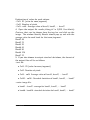
-The input is a text file of the following format: Polygon id, land
cover class, land cover subclass, tree cover class, resolution of the
image in GE (Google Earth), year and month of image in GE. After
the ”:” mark there are corner coordinates in WGS84 system. - This
input data can be output from another script, GExml2csv.bash and
originally derives from a training data collection tool created for GE.
User Manual
12
EXAMPLE
For this exercise following tools are used: CsvToPolygon.py
Open your working directory using
cd /home / . . .
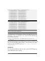
An example of the beginning of input data is following:
106,OWL,OWL Open,2,Coarse,2002/1:-5.47450324983224 32.54081338469396,5.47450324983224
32.5417154317423,-5.47540856036825 32.5417154317423,-5.47540856036825
32.54081338469396
107,Grassland,Grassland Bushed,1,Coarse,2002/1:-5.47456561893842
32.63108751846197,-5.47456561893842 32.63198971163985,-5.47547080384603
32.63198971163985,-5.47547080384603 32.63108751846197
108,Bushland,Bushland Thicket,2,Medium,2002/10:-5.47461439045748
32.72136258245697,-5.47461439045748 32.72226491949511,-5.47551944746972
32.72226491949511,-5.47551944746972 32.72136258245697
This is how you run the command:
p y t h o n CsvToPolygon . py i n p u t d a t a . c s v o u t p u t . shp
User Manual
13
7.2
genericCsvToPolygon.py
NAME
GenericCsvToPolygon.py - Program for creating polygons from text
files
OFGT VERSION
1.25.4
SYNOPSIS genericCsvToPolygon.py
genericCsvToPolygon.py <input.csv><output.shp>
DESCRIPTION
GenericCsvToPolygon.py Program for creating polygons from text
files.
- The input file is a text file of the following format: Polygon id:corner
coordinates in WGS84 system
- Coordinate pairs are separated from others with a space and x,y
with a comma, see under EXAMPLE:
NOTES
The program is modified form the one by Chris Garrard:
http://www.gis.usu.edu/~chrisg/python/2009/lectures/ospy_
hw2a.py
SEE ALSO
This input data is output from another script, genericGEkml2csv.bash
and originally comes from Google Earth (self-digitized polygon
kml’s).
EXAMPLE
The input file is a text file of the following format: Polygon id:corner
coordinates in WGS84 system
User Manual
14
Bushland1 :38.99408253760913 , −11.04146530113384 ,0
38.99380823486723 , −11.04205402821617 ,0
38.99380826389991 , −11.04206992654894 ,0
38.99382544867113 , −11.04261044223288 ,0
38.9938254776416 , −11.04262634062336 ,0
38.99415014990515 , −11.04300732377466 ,0
38.9941664064954 , −11.04303909164155 ,0
38.99466885692982 , −11.04319717791531 ,0
38.99473365203311 , −11.04319706202726 ,0
38.99479844656671 , −11.0431969461398 ,0
38.99515464117336 , −11.04310091874687 ,0
38.99518697983437 , −11.04306906417552 ,0
bushland2 :39.00340243948988 , −11.04234996851613 ,0
39.00296537982829 , −11.04267663255115 ,0
39.00290506714792 , −11.04270636631092 ,0
39.00271044958266 , −11.04355103802362 ,0
39.00271058813281 , −11.04362510127527 ,0
39.00308922316352 , −11.04433543402553 ,0
39.0031345553759 , −11.04436497858972 ,0
39.00316485086498 , −11.04442417551431 ,0
39.00373863444808 , −11.04457127447502 ,0
39.00378391140981 , −11.04457119324793 ,0
Then run the actual command:
g e n e r i c C s v T o P o l y g o n . py i n p u t . c s v o u t p u t . shp
The output shp is in geographic WGS84, but does not carry that
information. You can transform it e.g. into UTM 36S WGS84 with
the following command:
o g r 2 o g r − s s r s EPSG : 4 3 2 6 − t s r s EPSG : 3 2 7 3 6 p r o j o u t p u t . shp
o u t p u t . shp
Where EPSG:4326 stands for WGS84 (source system) and EPSG:32736
for UTM 36S WGS84 (target system). You can select any target
system and find the EPSG code, see http://spatialreference.
org/ref/epsg/
EXAMPLE
For this exercise following tools are used: genericCsvToPolygon.py,
genericGEkml2csv.bash, ogr2ogr
User Manual
15
This script performs conversion from a set of generic .kml format polygons created in Google Earth (GE) into one combined
textfile. This textfile can then be converted into a shapefile using
script genericCsvToPolygon.py
• How to create polygons in Google Earth and save them as .kml
files
• Then open your working directory using
cd /home / . . .
The procedure is:
1. Put the kml’s into one folder
2. Launch genericGEkml2csv.bash in that kml-folder. This creates
a csv file ”output.csv”
genericGEkml2csv . bash
3. Launch genericCsvToPolygon.py in the same folder, with parameters as follows:
g e n e r i c C s v T o P o l y g o n . py o u t p u t . c s v o u t p u t . shp
The shapefile name can be as you wish (e.g. settlements168063.shp).
The shapefile is in geographic WGS84, but does not carry that information. You can transform it e.g. into UTM 36S WGS84 with the
following command - Input: output.shp; Output: proj output.shp:
o g r 2 o g r − s s r s EPSG : 4 3 2 6 − t s r s EPSG : 3 2 7 3 6 p r o j o u t p u t . shp
o u t p u t . shp
Where EPSG:4326 stands for WGS84 (source system) and EPSG:32736
for UTM 36S WGS84 (target system). You can select any target system and find the EPSG code, see http://spatialreference.org/ref/epsg/
User Manual
16
7.3
genericGEkml2csv.bash
NAME
genericGEkml2csv.bash - converts separate kml files from Google
Earth into one CSV file.
OFGT VERSION
1.25.4
SYNOPSIS genericGEkml2csv.bash
DESCRIPTION
genericGEkml2csv.bash converts separate kml files from Google
Earth (GE) into one CSV file.
This script performs conversion from a set of generic .kml format
polygons created in GE into one combined textfile.
NOTES
All kml files need to be in one folder from where the script needs to
be launched
SEE ALSO
The output textfile of genericGEkml2csv.bash can then be converted
into a shapefile using script genericCsvToPolygon.py.
EXAMPLE
1. Put all kml files into one folder
2. Launch genericGEkml2csv.bash in that kml-folder. This creates
a csv file ”output.csv”
genericGEkml2csv . bash
// no need t o d e f i n e i n p u t o u t p u t
3. Look into your working directory and see if output.csv was
created. Take a closer look at its first lines:
head o u t p u t . c s v
User Manual
17
3. Conversion of output.csv into a shapefile: Launch genericCsvToPolygon.py in the same folder, with parameters as follows:
g e n e r i c C s v T o P o l y g o n . py o u t p u t . c s v o u t p u t . shp
The shp name can be as you wish (e.g. settlements168063.shp).
4. The shapefile is in geographic WGS84, but does not carry that information. You can transform it e.g. into UTM 36S WGS84 with the
following command (Input: output.shp; Output: proj output.shp).
o g r 2 o g r − s s r s EPSG : 4 3 2 6 − t s r s EPSG : 3 2 7 3 6 p r o j o u t p u t . shp
o u t p u t . shp
Where EPSG:4326 stands for WGS84 (source system) and EPSG:32736
for UTM 36S WGS84 (target system). You can select any target
system and find the EPSG code, see http://spatialreference.
org/ref/epsg/
User Manual
18
7.4
GExml2csv.bash
NAME
GExml2csv.bash - converts xml files from Google Earth training data
collection tool into one CSV file.
OFGT VERSION
1.25.4
SYNOPSIS GExml2csv.bash
DESCRIPTION
GExml2csv.bash converts single files originating from Google Earth
(GE) training data collection tool into a combined CSV file.
NOTES
The script is to be launched in a directory containing the target xml’s
EXAMPLE
For this exercise following tools are used: GExml2csv.bash
Open your working directory where you stored you xml files using
cd /home / . . .
hen simply run following command:
GExml2csv . b a s h
User Manual
19
7.5
oft-addattr.py
NAME
oft-addattr.py - adds one integer attribute in a shape file.
OFGT VERSION
1.25.4
SYNOPSIS oft-addattr.py
oft-addattr.py <shapefile><JoinAttrName><NewAttrName><textfile>
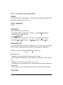
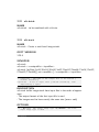
DESCRIPTION
oft-addattr.py adds one integer attribute in a shape file:
oft-addattr.py reads a space separated text file and uses the first
and second columns to construct a lookup table which is used to add
a new attribute in an existing shapefile. Each time the value in the
first column is found in the JoinAttributeName field of the shapefile,
the value in the second column is added in the field NewAttrName.
In case the corresponding value is not present in the textfile, the
NewAttrName value for that record becomes -9999.
NOTES
The values need to be in integer!
EXAMPLE
-For this exercise following tools are used: oft-addattr.py
- You might have created it already in exercise in the OFGT wikipedia
’How to create and export polygons from Google Earth (GE)’.
- Open your working directory using
cd /home / . . .
- The first lines of the attribute table of landuse.shp look like this:
1 red
2 green
User Manual
20
3 orange
5 pink
6 red
7 blue
8 orange
9 green
10 o r a n g e
- In this exercise we create a space separated text file as a lookup
table. You can create it in any text editor, such as gedit or kate
and save the file as lookup.txt in your working directory.
Note: The first column contains the ID linking the lookup table to
your shapefile and the second column contains the values you want
to add to the new column of your shapefile.
1 11
2 22
3 33
4 44
5 55
6 66
8 88
9 99
10 1000
- Now run the script in the command line.
Each time the value in the first column of lookup.txt is found in the
JoinAttributeName of the landuse.shp, field in our case called id.
The value in the second column is added in the field NewAttrName,
here called newcol. Note: The values need to be in integer! How
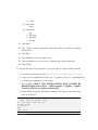
to change the data type in QGIS see further down.
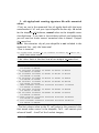
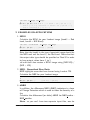
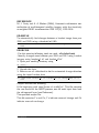
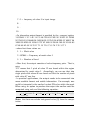
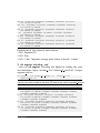
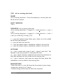
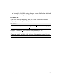
o f t −a d d a t t r . py
l a n d u s e . shp i d n e w c o l l o o k u p . t x t
- Load landuse.shp in QGIS and look at your attribute table. You
should now find the new column called newcol with it values.
- Take a look at the ID 7. The newcol value in landuse.shp is -9999.
This is due to the fact that there was no value 7 in the first column
of the lookup table. In that case the corresponding value is not
present in the lookuptable, therefore the newcol value for that record
becomes -9999.
User Manual
21
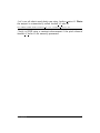
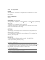
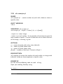
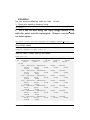
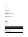
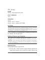
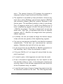
Figure 1: Attribute table of landuse.shp containing the new column called newcol
with values.
HOW TO CHANGE THE DATA TYPE OF THE VALUES
IN THE ATTRIBUTE TABLE IN QGIS
Add plugin Table Manager:
1. Click on the top bar’Plugins’ ->click ’Fetch Python Plugins’.
2. Type in the filter ’Manager’ ->then you should find ’Table
Manager - Manages the attribute table structure’.
3. Install it. Close and re-open QGIS.
4. On top bar click ’Plugin’ ->click ’Manage Plugins’ ->tick box
for ’Table Manager’.
5. On top bar click ’Plugin’ ->you should now see ’Table’ somewhere under ’Manage Plugins’, click it and the option ’Table
Manager’ can be chosen.
6. From there you can edit your attribute table, add a new colum
and choose the data type.
User Manual
22
7.6
oft-addpct.py
NAME
oft-addpct.py - adds pseudo color table to an image.
OFGT VERSION
1.25.4
SYNOPSIS oft-addpct.py
oft-addpct.py <inputfile><outputfile>
DESCRIPTION
oft-addpct.py adds a pseudo color table to an image keeps the
original values of the image, but ensures that classes are shown in
pre-defined colors, no matter which application is used to open the
image.
After defining the first line, the command will ask for the text
file containing the color table:
Give LUT file name: <colortable>
Where:
- <inputfile>is an image file
- <outputfile>is an image file (if it is the same as <inputfile>,
<inputfile>will be overwritten)
- <colortable>is a text file with 4 or 5 columns containing the color
table in the following format:
• 1st column: class value
• 2nd - 4th column: RGB values
• optional: 5th column for alpha, if not set, it is assumed to be
255
• Important: The <colortable>must NOT contain any empty
lines!
User Manual
23
• see Wikipedia for more information on RGBA color space.
The <colortable>could look like this:
1
2
3
4
103 51 1 255
254 0 0 255
0 0 254 255
0 255 0 255
EXAMPLE
- For this exercise following tools are used: oft-addpct.py
- Create the colortable for the file images/forestc.tif. If you do not
know which classes are present in images/forestc.tif, you could use
oft-stat with images/forestc.tif both as input and mask file. The
first column of the mask file shows all present classes (besides 0).
Create a text file called txt/coltable.txt, with the first column
indicating all possible classes. It could look like this:
1 0 0 0 0
44 122 122 0 255
33 103 51 1 255
55 4 253 255 255
22 122 0 122 255
11 255 0 0 255
4 122 122 122 255
3 255 255 0 255
2 200 200 200 255
6 0 255 0 255
Important: Make sure that the text file does not contain any empty
lines.
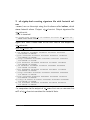
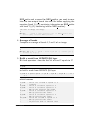
- Run oft-addpct.py:
o f t −a d d p c t . py i m a g e s / f o r e s t c . t i f
results/forestcolor . tif
- The command will ask you about the colortable file:
G i v e LUT f i l e name
Enter the path to your color table file and hit enter:
txt / coltable . txt
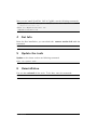
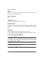
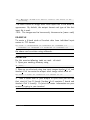
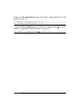
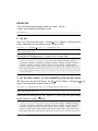
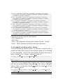
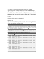
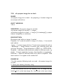
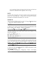
- You can visualize the result in QGIS:
qgis results / forestcolor . t i f
User Manual
24
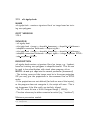
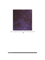
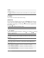
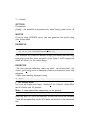
Figure 2: Example of using oft-addpct.py to define the colour table.
User Manual
25
7.7
oft-admin-mask.bash
NAME
oft-admin-mask.bash - this script prepares a mask of administrative
areas within a satellite image.
OFGT VERSION
1.25.4
SYNOPSIS oft-admin-mask.bash
oft-admin-mask.bas <mask for Landsat image><administrative
area image>[ID of wanted administrative area]
DESCRIPTION
- If no ID is given the script just clips and re-projects (if needed) the
admin image to match the Landsat image mask
- If an ID is given, the admin area with this ID is added to the base
mask and other areas are set to 0
- The input administrative image does not need to be of the same
size and projection (script utilises oft-clip.pl for clipping and reprojecting)
EXERCISE
- For this exercise following tools are used: oft-admin-mask.bash,
oft-shptif.bash
- Open your working directory using
cd /home / . . .
- In a first step we need to prepare an image with administrative areas
using oft-shptif.bash. For exercise purpose we simply use landuse.shp
as an input for hypothetical admin areas. Output: landuse raster.tif
o f t −s h p t i f . b a s h l a n d u s e . shp l a n d s a t t 1 . t i f l a n d u s e r a s t e r . t i f
landuse
User Manual
26
- Let’s run oft-admin-mask.bash now using landuse raster.tif. Note:
the output is automatically called landsat t1 adm.tif.
o f t −admin−mask . b a s h l a n d s a t t 1 . t i f l a n d u s e r a s t e r . t i f
- Verify in QGIS using a contrast enhancement if the pixel values of
landsat t1 adm.tif are correctly processed.
User Manual
27
7.8
oft-bb
NAME
oft-bb - is a a bounding box calculator t.
OFGT VERSION
1.25.4
SYNOPSIS oft-bb
oft-bb [-um maskfile] <inputfile><value>
DESCRIPTION
oft-bb studies every pixel of the input file and reports minimum
and maximum pixels coordinates of pixels having the given value.
The minimum coordinates are 1,1. - <inputfile>is an image file
- <value>is the value you want to query
- -um use mask file. It will consider only pixels which have mask
value >0
EXERCISE
- For this exercise following tools are used: oft-bb, gdal translate
- Open your working directory using
cd /home / . . .
- Find the bounding box of the Forest tree cover file forestc.tif with
value ”33”
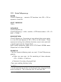
o f t −bb i m a g e s / f o r e s t c . t i f 33
- It should provide the following result :
Band 1 BB ( xmin , ymin , xmax , ymax ) i s 1408 1740 1713 1964
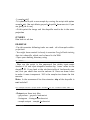
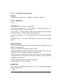
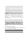
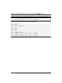
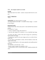
- You can visualize the result by subsetting the image to these extents
using gdal translate
g d a l t r a n s l a t e −s r c w i n 1408 1740 305 224 i m a g e s / f o r e s t c . t i f
r e s u l t s / bb 33 . t i f
User Manual
28
The parameters for the size of the box are calculated as xmax-xmin
and ymax-ymin
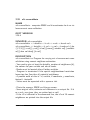
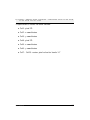
Visualize the results
q g i s images / f o r e s t c . t i f
r e s u l t s / bb 33 . t i f
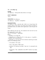
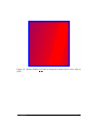
Figure 3: Example of using oft-bb output bb 33.tif.
User Manual
29
7.9
oft-classvalues-compare.bash - To be tested
NAME
oft-classvalues-compare.bash - creates comparison plots of classes
based on result of previous script oft-classvalues-plot.bash.
OFGT VERSION
1.25.4
SYNOPSIS oft-classvalues-compare.bash
oft-classvalues-compare.bash <class1><class2>
oft-classvalues-compare.bash <class1><class2>[class3] [class4] [class5]
DESCRIPTION
oft-classvalues-compare.bash This script is meant to be used after
script oft-classvalues-plot.bash. It plots 2-5 classes in the same
figure and the distinction of classwise point clouds can be evaluated.
- It is launched in the folder containing classwise plots and text files
produced by the above mentioned script.
OPTION
Additional classes that can be plotted in the same figure:
Parameters:
- [class3]
- [class4]
- [class5]
SEE ALSO
Look at oft-classvalues-plot.bash, which computes input data for
this tool
EXAMPLE
User Manual
30
- For this exercise following tools are used: oft-classvalues-plot.bash
- Input data deriving from exercise oft-classvalues-plot.bash
- Change your working directory to the one of the previous exercise
oft-classvalues-plot.bash:
cd /home / . . .
- Use oft-classvalues-compare to create a comparison plot of band2
and band3.
Output to be found in folder plots LT52 CUB00.tif bands 3 4 created after running oft-classvalues-plot.bash.
Output: Comparison1 3.png
o f t −c l a s s v a l u e s −compare . b a s h 1 3
User Manual
31
- Now compare band1, band2 and band3; Output: Comparison1 2 3.png
o f t −c l a s s v a l u e s −compare . b a s h 1 2 3
User Manual
32
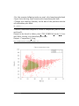
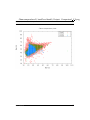
7.10
oft-classvalues-plot.bash - To be tested
NAME
oft-classvalues-plot.bash - creates scatterplots of pixels within training classes (given in a shapefile).
OFGT VERSION
1.25.4
SYNOPSIS oft-classvalues-plot.bash
oft-classvalues-plot.bash <input image><shapefile basename>
<shapefile class fieldname><image band for x-axis><image band
for y-axis>
DESCRIPTION
oft-classvalues-plot.bash This script creates scatterplots of image
grey values in different classes of training data. Also figures of class
means and standard deviations are provided.
- Training areas need to be in shapefiles.
- The figures of class means and std’s for both required bands are
created in the launching folder (.png format).
- It also puts the class means and standard deviations into text files.
- Pixel-by-pixel values are stored in a separate text file.
- The pixel plots are created in a folder named plots imagename band1 band2.
They are for all classes, .png image files. And same as text files.
NOTES
Make sure that you have installed GNUPLOT.
SEE ALSO
A further script oft-classvalues-compare.bash can then be used to
compare up to 5 classes in one view.
User Manual
33
EXAMPLE
- For this exercise following tools are used: oft-classvalues-plot.bash Input data: download for this exercise the Landsat imagery landsat t1.tif
and the shapefile: landuse.shp
- Open your working directory using
cd /home / . . .
- First of all make sure that you have installed textbfGNUPLOT.
Further information on Gnuplot and Ubuntu. If you don’t have
Gnuplot type in your terminal:
sudo apt−g e t i n s t a l l g n u p l o t // p r e s s ’ e n t e r ’
- Run oft-classvalues-plot.bash with input: satellite image k shapefile
k Attribute column for ID in this case name k band3 k band4; Input
image: landsat t1.tif, input shapefile: landuse.shp; Note: the output
is automatically processed.
o f t −c l a s s v a l u e s −p l o t . b a s h l a n d s a t t 1 . t i f l a n d u s e name 3 4
Output:
1. pixelvalueslandsat t1.tif bands 3 4.txt:
head p i x e l v a l u e s l a n d s a t t 1 . t i f b a n d s 3 4 . t x t
Column 1-6: Pixel ID, X , Y , class (from attribute name), pixelvalue bandnr3,
pixelvalue bandnr4
1.00
2.00
3.00
4.00
5.00
771870.00
771900.00
771930.00
771960.00
771990.00
−2402010.00
−2402010.00
−2402010.00
−2402010.00
−2402010.00
6.00
6.00
6.00
6.00
6.00
22.00
22.00
23.00
22.00
21.00
47.00
53.00
55.00
55.00
53.00
2. classvalues landsat t1.tif band 3.txt:
head c l a s s v a l u e s l a n d s a t t 1 . t i f b a n d 3 . t x t
Column 1-3: classvalue, bandnr3 , std
User Manual
34
7 27.224344 2.480986
13 2 8 . 9 4 5 9 4 6 1 . 6 7 9 2 0 5
8 28.140811 2.322499
9 29.036641 2.258223
12 2 7 . 8 7 9 4 6 4 1 . 2 8 8 0 4 9
11 2 7 . 4 2 3 6 9 5 1 . 1 9 9 9 3 3
3. classvalues landsat t1.tif band 4.txt
head c l a s s v a l u e s l a n d s a t t 1 . t i f b a n d 3 . t x t
Column 1-3: classvalue, bandnr4 , std
7 48.176611 2.622561
13 4 5 . 3 8 5 7 4 9 1 . 5 2 5 1 8 9
8 49.842482 2.397968
9 52.786260 3.513642
12 4 9 . 9 4 3 4 5 2 2 . 2 3 2 3 5 0
11 4 8 . 7 7 9 1 1 6 1 . 1 7 2 8 8 5
4. Folder plots landsat t1.tif bands 3 4 contains the classes to be
used for oft-classvalues-compare.bash.
User Manual
35
7.11
oft-combine-masks.bash
NAME
oft-combine-masks.bash - combines several masks (raster and shapefiles) to one mask file
OFGT VERSION
1.25.4
SYNOPSIS oft-combine-masks.bash
oft-combine-masks.bash <input1><input2>.... <nodata>
oft-combine-masks.bash <input1><input2>.... <nodata>[EPSG
code]
DESCRIPTION
oft-combine-masks.bash is a UNIX bash script that allows the user
to use both mask images and mask shapefiles as input and the script
combines them into one mask file.
- The first inputfile is the base and it must be an image not shapefile
- The following input files will be written on only if there is nodata
(user-defined value)
- The extent is defined by the first input image
- If the projection is not given by the user, all files are assumed to
be in same projection
- Concerning the shapefiles, the last field is assumed to be the one
containing the mask values
- At least 2 files and nodata value are needed
OPTION
The projection can be defined by the user.
Parameters:
[EPSG code]
User Manual
36
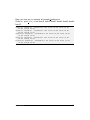
EXAMPLE
- For this exercise following tools are used: oft-combine-masks.bash,
oft-calc, gdal rasterize - Open your working directory using
cd /home / . . .
STEP 1: CREATE MASKS
- To run oft-combine-masks.bash we need to create some mask files.
To do so, we burn the attribute values of the column mask from
the shapefile landuse.shp into the raster forestc.tif :
g d a l r a s t e r i z e −b 1
forest . tif
−a mask
− l l a n d u s e l a n d u s e . shp f o r e s t c . t i f
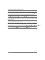
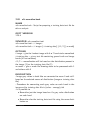
- Verify in QGIS if your pixel values of forestc.tif match the polygon
values of landuse.shp.
- Note: if the raster output is black, click on it’s Properties ->Style
->Colour Map and chose Pseudo Colour
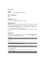
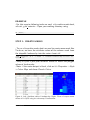
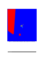
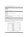
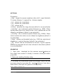
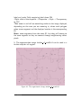
Figure 4: Left: Attribute table of landuse.shp. Right: Zoom of output raster
forestc.tif in QGIS using the colourmap Pseudocolour.
User Manual
37
- Forestc.tif is the base raster to create some masks files by
extracting those pixels that contain values which were previously in
the shapefile and then burned into the raster:
o f t −c a l c f o r e s t c . t i f mask1 . t i f
1
#1 55 = 0 1 ?
// I f t h e p i x e l v a l u e s i s 55 i n f o r e s t c . t i f , t h e n
g i v e i t i n mask1 . t i f t h e v a l u e 1 , o t h e r w i s e 0
o f t −c a l c f o r e s t c . t i f mask2 . t i f
1
#1 11 = 0 2 ?
// I f t h e p i x e l v a l u e s i s 11 i n f o r e s t c . t i f , t h e n
g i v e i t i n mask2 . t i f t h e v a l u e 2 , o t h e r w i s e 0
o f t −c a l c f o r e s t c . t i f mask3 . t i f
1
#1 33 = 0 3 ?
// I f t h e p i x e l v a l u e s i s 33 i n f o r e s t c . t i f , t h e n
g i v e i t i n mask3 . t i f t h e v a l u e 3 , o t h e r w i s e 0
o f t −c a l c f o r e s t c . t i f mask4 . t i f
1
#1 44 = 0 4 ?
// I f t h e p i x e l v a l u e s i s 44 i n f o r e s t c . t i f , t h e n
g i v e i t i n mask4 . t i f t h e v a l u e 4 , o t h e r w i s e 0
o f t −c a l c f o r e s t c . t i f mask5 . t i f
1
#1 22 = 0 5 ?
// I f t h e p i x e l v a l u e s i s 22 i n f o r e s t c . t i f , t h e n
g i v e i t i n mask5 . t i f t h e v a l u e 5 , o t h e r w i s e 0
- Again, check in QGIS if the masks contain the extracted value for
the same location of the corresponding polygon in landuse.shp.
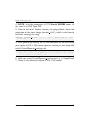
- In the final step we run the command oft-combine-masks.bash.
Note that output file is automatically processed called combinedmask.img
o f t −combine−masks . b a s h mask1 . t i f mask2 . t i f mask3 . t i f mask4 . t i f
mask5 . t i f 0
User Manual
38
STEP 2: COMBINE MASKS USING RASTER AND SHAPEFILE
- Run oft-combine-masks.bash: Input: mask1.tif, mask2.tif, mask3.tif,
mask4.tif, mask5.tif and the additional shapefile clouds.shp In the
shapefile the values of the last column are picked up for processing;
output is automatically processed: combined-masks.img
textbfNOTE: copy your combined-mask.img output from the first
exercise as it will be overwritten running oft-combine-masks.bash
again.
c o m b i n e m a s k s . b a s h mask1 . t i f mask2 . t i f mask3 . t i f mask4 . t i f mask5
. t i f c l o u d s . shp 0 // t h e 0 d e f i n e s n o d a t a v a l u e s t o be 0
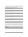
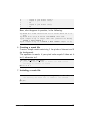
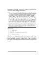
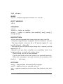
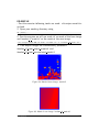
- Verify in QGIS if combined-masks.img contains all mask values,
and if the additional polygon of clouds.shp has the values 99 (look
into attribute table of clouds.shp under the last column).
User Manual
39
Figure 5: Combined masks including the larger polygon from clouds.shp.
User Manual
40
7.12
oft-compare-overlap.bash - To be tested
NAME
oft-compare-overlap.bash - This script compares overlapping areas
of 2 images and produces between-band correlations.
OFGT VERSION
1.25.4
SYNOPSIS oft-compare-overlap.bash
oft-compare-overlap.bash <image1.img><image2.img><mask1.img>
<mask2.img><grid spacing>[EPSG:img1]
- Give the spacing in metres (1000 = 1 km)
- Give the last parameter in format EPSG:32637 (replace number
with your own, this is for UTM 37 N)
DESCRIPTION
- Meant for evaluation of the brdf correction of 2 images, but other
imagery can be compared as well
- The second image is projected to the same projection as the first,
if the projections differ
- In that case, user gives the projection of first image ad EPGS code.
And both images need to have a projection defined (although it
differs)
- Similar number of bands must exist
- Masks must be given for both images to exclude cloud/shadow
areas
- They must be of same size and in same projection as their corresponding images
- Only areas where mask has value 2 are used in comparison (you
may give a mask full of 2 if needed)
- User gives the spacing of the sampling points as well
User Manual
41
EXAMPLE
- For this exercise following tools are used: oft-compare-overlap.bash,
oft-calc, gdal translate, oft-trim-mask.bash
- Open your working directory using
cd /home / . . .
- Convertlandsat t1.tif into 6 bands as both need to have same nr
of bands. Output: landsat t1 6bands.tif
g d a l t r a n s l a t e l a n d s a t t 1 . t i f l a n d s a t t 1 6 b a n d s . t i f −b 1 −b 2 −
b 3 −b 4 −b 5 −b 6
- Create mask for landsat t1 6bands.tif ;
automatic output:landsat t1 6bands mask.tif
o f t −t r i m −mask . b a s h l a n d s a t t 1 6 b a n d s . t i f
- NOTE: the mask value to be used is 2, so conversion of mask from
value 1 to 2: input: landsat t1 6bands mask.tif ; output: mask1.tif
o f t −c a l c l a n d s a t t 1 6 b a n d s m a s k . t i f mask1 . t i f
1
#1 1 = 0 2 ?
- Create mask for landsat t2 ; automatic output: landsat t2 mask.tif
o f t −t r i m −mask . b a s h l a n d s a t t 2 . t i f
- Convert mask value to 2: landsat t2 mask.tif ; output: mask2.tif
o f t −c a l c l a n d s a t t 2 m a s k . t i f mask2 . t i f
1
#1 1 = 0 2 ?
- Run oft-compare-overlap.bash
o f t −compare−o v e r l a p . b a s h l a n d s a t t 1 6 b a n d s . t i f l a n d s a t t 2 . t i f
mask1 . t i f mask2 . t i f
1000
- Output: img12mask12 sed.txt printed on screen:
head i m g 1 2 m a s k 1 2 s e d . t x t
3 2 9 . 0 0 7 3 2 2 8 5 . 0 0 −2447885.00 1 0 0 . 0 0 3 1 6 6 . 0 0 2 . 0 0 2 . 0 0 1 0 0 . 0 0
3166.00 2.00 2.00 100.00 3166.00 53.00 25.00 27.00 48.00
71.00 131.00 53.00 25.00 27.00 48.00 71.00 131.00 100.00
3166.00 66.00 60.00 66.00 88.00 98.00 69.00 66.00 60.00 66.00
88.00 98.00 69.00
User Manual
42
3 3 0 . 0 0 7 3 2 2 8 5 . 0 0 −2446885.00 1 0 0 . 0 0 3 1 3 3 . 0 0 2 . 0 0 2 . 0 0 1 0 0 . 0 0
3133.00 2.00 2.00 100.00 3133.00 54.00 25.00 27.00 48.00
71.00 128.00 54.00 25.00 27.00 48.00 71.00 128.00 100.00
3133.00 61.00 53.00 51.00 100.00 77.00 49.00 61.00 53.00
51.00 100.00 77.00 49.00
3 3 1 . 0 0 7 3 2 2 8 5 . 0 0 −2445885.00 1 0 0 . 0 0 3 1 0 0 . 0 0 2 . 0 0 2 . 0 0 1 0 0 . 0 0
3100.00 2.00 2.00 100.00 3100.00 56.00 25.00 29.00 53.00
73.00 128.00 56.00 25.00 29.00 53.00 73.00 128.00 100.00
3100.00 67.00 61.00 66.00 95.00 89.00 65.00 67.00 61.00
66.00 95.00 89.00 65.00
3 3 2 . 0 0 7 3 2 2 8 5 . 0 0 −2444885.00 1 0 0 . 0 0 3 0 6 6 . 0 0 2 . 0 0 2 . 0 0 1 0 0 . 0 0
3066.00 2.00 2.00 100.00 3066.00 46.00 19.00 17.00 40.00
41.00 124.00 46.00 19.00 17.00 40.00 41.00 124.00 100.00
3066.00 55.00 44.00 36.00 80.00 53.00 25.00 55.00 44.00
36.00 80.00 53.00 25.00
3 3 3 . 0 0 7 3 2 2 8 5 . 0 0 −2443885.00 1 0 0 . 0 0 3 0 3 3 . 0 0 2 . 0 0 2 . 0 0 1 0 0 . 0 0
3033.00 2.00 2.00 100.00 3033.00 46.00 20.00 18.00 39.00
45.00 124.00 46.00 20.00 18.00 39.00 45.00 124.00 100.00
3033.00 56.00 43.00 35.00 81.00 56.00 26.00 56.00 43.00
35.00 81.00 56.00 26.00
3 3 4 . 0 0 7 3 2 2 8 5 . 0 0 −2442885.00 1 0 0 . 0 0 3 0 0 0 . 0 0 2 . 0 0 2 . 0 0 1 0 0 . 0 0
3000.00 2.00 2.00 100.00 3000.00 48.00 20.00 18.00 36.00
42.00 125.00 48.00 20.00 18.00 36.00 42.00 125.00 100.00
3000.00 55.00 43.00 35.00 77.00 54.00 27.00 55.00 43.00
35.00 77.00 54.00 27.00
User Manual
43
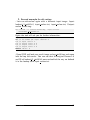
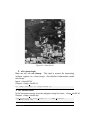
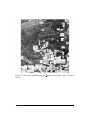
Figure 6: Output of oft-compare-overlap.bash visualized in QGIS.
User Manual
44
7.13
oft-crop.bash
NAME
oft-crop.bash - crops a raster image to the extent of a certain pixel
value.
OFGT VERSION
1.25.4
SYNOPSIS oft-crop.bash
oft-crop.bash <input-img><output-img>[ value / -all ] [ nodatavalue ]
OPTION
- [ value / -all ]: [value] = is the value of the inputfile it should be
cropped to -all = if image should be cropped to every unique pixel
value; output will be named accordingly
- [nodata-value]: for this value no cropping will be done; if not
provided, it is assumed to be 0 (only applicable for option -all)
DESCRIPTION
- Oft-crop.bash crops a raster image to the extent of a certain pixel
value. This can be useful when, for example, one wants to produce
a separate raster image for every district of a country.
- Input image is a raster image with unique pixel values for each
region of interest.
- In the output image, the value for the region of interest is kept.
All other pixels are set to 0.
- The user can choose to either:
• do the cropping for one single pixel value
• do the cropping for all occurring pixel values besides the nodatavalue. The nodata-value can be specified with the [nodata]option. If not specified, it is assumed to be 0. In this case,
User Manual
45
output files will carry the value they have been cropped to in
their name.
EXAMPLE
- For this exercise following tools are used: oft-crop.bash, gdal rasterize
- Open your working directory using
cd /home / . . .
- You will need for this exercise the file landuse.shp, digitized manually with QGIS
- Create a raster file that has the landuse class attribute of the
landuse.shp file
g d a l r a s t e r i z e −a n e w c o l − l l a n d u s e − t r 30 30 s h a p e f i l e s / l a n d u s e
. shp r e s u l t s / l a n d u s e . t i f
- Extract one particular class (in that case the zone that has the
label 2000)
o f t −c r o p . b a s h r e s u l t s / l a n d u s e . t i f
User Manual
r e s u l t s / l u c l a s s . t i f 2000
46
7.14
oft-cuttile.pl
NAME
oft-cuttile.pl - Cuts image tiles on the basis of a given list of locations
OFGT VERSION
1.25.4
SYNOPSIS oft-cuttile.pl
oft-cuttile.pl <coord list><CRS file><input dir><output basename>
OPTIONS
- <coord ist>is a text file containing the coordinates of the center
of the tiles. It must arranged as id x y
- <CRS file>is a text file containing the projection definitions of
the dataset in PROJ4 format.
- <input dir>is the directory containing the image. Image must be
in geotiff format, extension must be .TIF with capitals.
- <output basename>is the base name of the tiles that will be
generated
DESCRIPTION
oft-cuttile.pl Cuts image tiles on the basis of a given list of locations.
1. converts the point locations into the projection of the image,
2. cuts a set of 20 km x 20 km tiles around the locations
3. converts the tiles to the coordinate system of the points (20 km
x 20 km)
EXAMPLE
- For this exercise following tools are used: oft-cuttile.pl, gdal translate,
cs2cs
- Open your working directory using
User Manual
47
cd /home / . . .
1. First, we need to convert the imagery into .TIF format. You
can use the gdal translate function to convert your input imagery
from any gdal supported format to TIF using the option [-of GTiff]
input.your format output.TIF
g d a l t r a n s l a t e −o f G T i f f i m a g e s / l a n d s a t t 1 . t i f
l a n d s a t t 1 . TIF
results/
2. In the next step we take a closer look at our additional input
data coordinates.txt and proj.txt
- coordinates.txt is a space separated text file: col1: ID, col2: X,
col3: Y coordinates
gedit results / coordinates . txt
Then copy paste the following list and save your file.
1
2
3
4
767360
755310
781072
789936
−2415219
−2378377
−2379346
−2440150
- proj.txt must contain one line with the projection definition of the
tiles coordinates and one line with the projection definition of the
imagery. Here it is UTM zone 20, for both, with the following proj4
format:
+ i n i t =e p s g : 3 2 6 2 0 +p r o j=utm +z o n e =20 +datum=WGS84 +u n i t s=m +
n o d e f s + e l l p s =WGS84
Create the file
gedit results / proj . txt
Paste the projection definition twice, as two separate lines. Save
proj.txt
+ i n i t =e p s g : 3 2 6 2 0 +p r o j=utm +z o n e =20 +datum=WGS84 +u n i t s=m +
n o d e f s + e l l p s =WGS84
+ i n i t =e p s g : 3 2 6 2 0 +p r o j=utm +z o n e =20 +datum=WGS84 +u n i t s=m +
n o d e f s + e l l p s =WGS84
User Manual
48
NB: If you do not have it, you can get the PROJ4 format of an
image by using the function cs2cs
c s 2 c s −v + i n i t =e p s g : 3 2 6 2 0
- If you don’t know the EPSG code of your image use gdalinfo for
your imagery:
g d a l i n f o l a n d s a t t 1 . TIF
5. Now we run the actual script to create the tiles in the terminal.
Output: Tiles
cd r e s u l t s
oft −c u t t i l e . p l c o o r d i n a t e s . t x t p r o j . t x t . T i l e s
User Manual
49
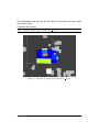
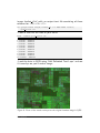
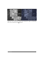
Figure 7: The four tiles overlayed on base image, displayed with differing band
composition to base imagery.
User Manual
50
7.15
oft-filter
NAME
oft-filter - moving window filters
OFGT VERSION
1.25.4
SYNOPSIS oft-filter
oft-filter [-ot Byte/Int16/UInt16/UInt32/Int32/Float32/Float64/CInt16/CInt32
/CFloat32/CFloat64] [-h] [-x xdim] [-y xdim] [-c const] [-n nodata]
[-f filter][-v] <-i inputfile><-i inputfile>
OPTIONS
- [-x dim] Window size in x-direction (default=3)
- [-y dim] Window size in y-direction (default=3)
- [-c const] Constant used to multiply the resulting value
- [-n value] Input NoData value, ignored in calculation (Def. from
infile)
- [-v] Verbose
- [-f filter] Type of statistics to be computed (default=1):
0: mean
1: standard deviation
2: variance
3: skewness
4: rank
5: coefficient of variation: 100*std/mean
DESCRIPTION
oft-filter The program computes local statistics on values of a raster
within the zones of a moving window.
1. converts the point locations into the projection of the image,
User Manual
51
2. cuts a set of 20 km x 20 km tiles around the locations
3. converts the tiles to the coordinate system of the points (20 km
x 20 km)
EXAMPLE
- For this exercise following tools are used: oft-filter
- Open your working directory using
cd /home / . . .
- In the first exercise we want to create the standard deviation
for the moving window using the default window size and default
statistics (without defining -f). The output image is called std.tif:
o f t − f i l t e r − i l a n d s a t t 1 . t i f −o s t d . t i f
- Now we go through an example calculating the coefficient of
variation (100*std/mean) using the option -f 5. Output: coe var.tif
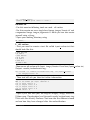
o f t − f i l t e r − i l a n d s a t t 1 . t i f −o c o e v a r . t i f −f 5 .
Calculation of the mean using the option -f 0. Output: mean.tif
o f t − f i l t e r − i l a n d s a t t 1 . t i f −o mean . t i f −f 0
Load your computed rasters in QGIS and verify your output statistics
using Identify Results.
User Manual
52
Figure 8: Example of the computed mean.tif
User Manual
53
7.16
oft-gengrid.bash
NAME
oft-gengrid.bash - generates a systematic grid over a raster image.
OFGT VERSION
1.25.4
SYNOPSIS oft-gengrid.bash
oft-gengrid.bash <input img><DX><DY><-output>
DESCRIPTION
oft-gengrid.bash generates a grid of points over an image (text
file), with user-defined spacing in x and y directions. Output is a
text file with the coordinates of the points. - Generates a text file
with 3 entries for each point: ID Xcoord Ycoord - <input img>is a
georeferenced input image
- <DX>is the distance between the points in X direction
- <DY>is the distance between the points in Y direction
- Prints the average, RMSE and bias on screen.
- Saves original value, estimate and difference in an output file. If id
or x and y are given, they are printed out as well.
- If the id is indicated in the command line, the id’s of 10 nearest
neighbours are printed into the output file.
EXAMPLE
- For this exercise following tools are used: oft-gengrid.bash
- Open your working directory using
cd /home / . . . / OFGT−d a t a
- Run the command line for generating the grid of 1000 x 1000
m distance between the points in X and Y directions on the input
User Manual
54
image landsat t1.tif with an output text file consisting of three
columns for <ID><X><Y>:
o f t −g e n g r i d . b a s h i m a g e s / l a n d s a t t 1 . t i f 1000 1000 r e s u l t s /
grid points . txt
- Look at the first ten lines of your result:
head
results / grid points . txt
1 730785 −2456134
2 730785 −2455134
3 730785 −2454134
4 730785 −2453134
5 730785 −2452134
6 730785 −2451134
7 730785 −2450134
8 730785 −2449134
9 730785 −2448134
10 730785 −2447134
- Load the data in QGIS using ’Add Delimited Text Layer’ and see
if it overlays on your Landsat image.
Figure 9: Zoom of the result overlayed on the original Landsat image in QGIS.
User Manual
55
7.17
oft-getcorners.bash
NAME
oft-getcorners.bash - gets the coordinates of corners of a raster
image or OGR vector layer .
OFGT VERSION
1.25.4
SYNOPSIS oft-getcorners.bash
oft-getcorners.bash <inputfile>[ -ul lr /-min max ]
OPTION
Where: <inputfile>is a GDAL raster layer or OGR vector layer
-ul lr = ulx uly lrx lry (default)
-min max = xmin ymin xmax ymax (ulx lry lrx uly)
DESCRIPTION
oft-getcorners.bash outputs the corner coordinates for a GDAL raster
layer or OGR vector layer.
The user can choose the order of the output:
- ulx: upper left x-coordinate
- uly: upper left y-coordinate
- lrx: lower right x-coordinate
- lry: lower right y-coordinate
EXAMPLE
- For this exercise following tools are used: oft-getcorners.bash
- Open your working directory using
cd /home / . . . / OFGT−d a t a
1. Run the oft-getcorners.bash:
o f t −g e t c o r n e r s . b a s h i m a g e s / l a n d s a t t 1 . t i f
User Manual
56
2. You should get the following output:
Not an OGR v e c t o r l a y e r
U s i n g GDAL r a s t e r l a y e r
Output i n o r d e r u l x u l y l r x l r y
7 2 9 2 8 5 . 0 0 0 −2352885.000 8 1 9 2 8 5 . 0 0 0 −2457885.000
User Manual
57
7.18
oft-polygonize.bash
NAME
oft-polygonize.bash - a wrapper for gdal polygonize.
OFGT VERSION
1.25.4
SYNOPSIS oft-polygonize.bash
oft-polygonize.bash <input.img><output.shp>
EXAMPLE
- For this exercise following tools are used: oft-polygonize.bash
- Open your working directory using
cd /home / . . . / OFGT−d a t a
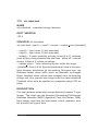
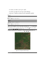
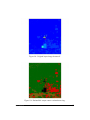
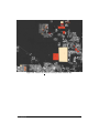
1. Let’s run oft-polygonize.bash using the input image landsat t1.tif
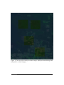
to create the output oft-polygonize.shp
o f t −p o l y g o n i z e . b a s h l a n d s a t t 1 . t i f o f t −p o l y g o n i z e . shp
2. Take a look at your shapefile in QGIS on go on propertiesof the
.shp ->Labels ->tick Display Labels, set Field Containing Label to
DN ->Press OK. The DN of each polygon in oft-polygonize.shp
should be the same as the pixel value of landsat t1.tif for the same
location.
User Manual
58
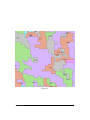
Figure 10: Zoomed view of oft-polygonize.shp.
User Manual
59
7.19
oft-sample-within-polys.bash
NAME
oft-sample-within-polys.bash - samples pixels within polygons and
generates training data for k-nn.
OFGT VERSION
1.25.4
SYNOPSIS
oft-sample-within-polys.bash
oft-sample-within-polys.bash <image><shapefile basename>
<shapefile class fieldname>
<size of sample>
oft-sample-within-polys.bash <image><shapefile basename>
<shapefile class fieldname><size of sample>[-sample only]
DESCRIPTION
oft-sample-within-polys.bash samples pixel values from an image
within areas determined by training data polygons (shapefile).
Output is named sample shapefile basename.txt
Specifications:
- Sample size (nbr of pixels) is given by the user
- The sample is distributed within classes in relation to class frequencies
- Output is a text file to be used e.g. in k-nn
- A histogram is also printed out, sample size per class is shown in
last column
- The image and the shapefile need to be in the same projection
OPTIONS
User Manual
60
- [-sample only]
- It is possible to pick a new sample by running the script with option
-sample only (do not delete greyvals shapefile basename.txt if you
are going to re-run)
- At this point the image and the shapefile need to be in the same
projection
OTHERS
Also look at oft-knn
EXAMPLE
- For this exercise following tools are used: oft-oft-sample-withinpolys.bash
- You might have created it already in exercise Google Earth training
data into shapefile, which can be found in the Wiki
- Open your working directory using
cd /home / . . .
- Now run the script in the command line within input-raster
landsat t1.tif and input-shapefile landuse.shp; ’name’ refers to the
shapefile ID. If you look at the attribute table of landuse.shp you
see, that you could also use the column id. Here we chose name
to make it more transparent. 100 is the sample size chosen for this
exercise.
Note: In the commmand line the extension .shp of the shapefile is
not included!
o f t −sample−w i t h i n −p o l y s . b a s h l a n d s a t t 1 . t i f l a n d u s e name 100
- Output are three text files:
- greyvalues - greyvals landuse.txt
- histogram - histogramlanduse.txt
- sample output - sample landuse.txt
User Manual
61
Here you can see an excerpt of sample landuse.txt
Order is: pixel id x y class band1 band2 band3 band4 band5 band6
band7:
1 0 5 5 7 . 0 0 7 7 2 6 5 0 . 0 0 −2404770.00 5 . 0 0 5 3 . 0 0 2 6 . 0 0 2 8 . 0 0 5 4 . 0 0
81.00 131.00 39.00
9 4 7 8 8 . 0 0 7 7 3 4 9 0 . 0 0 −2431680.00 1 . 0 0 5 1 . 0 0 2 4 . 0 0 2 5 . 0 0 4 5 . 0 0
65.00 127.00 33.00
2 0 1 5 3 6 . 0 0 7 7 4 7 5 0 . 0 0 −2439390.00 1 . 0 0 5 4 . 0 0 2 5 . 0 0 2 7 . 0 0 5 0 . 0 0
71.00 130.00 35.00
8 8 5 3 1 . 0 0 7 7 1 4 5 0 . 0 0 −2431110.00 1 . 0 0 4 7 . 0 0 2 1 . 0 0 1 8 . 0 0 3 7 . 0 0
48.00 126.00 21.00
1 2 3 3 7 4 . 0 0 7 7 4 1 5 0 . 0 0 −2433990.00 1 . 0 0 5 4 . 0 0 2 4 . 0 0 3 0 . 0 0 3 5 . 0 0
75.00 132.00 42.00
User Manual
62
7.20
oft-shptif.bash
NAME
oft-shptif.bash - Rasterizes a shapefile to the resolution of a reference image.
OFGT VERSION
1.25.4
SYNOPSIS oft-shptif.bash
oft-shptif.bash <shapefile><raster reference><raster output>[fieldname]
input files:
- shapefile that is supposed to be rasterized
- reference raster image - the shapefile will be rasterized to the same
extent and resolution of this image
OPTION
- [fieldname]: the fieldname of the attribute of the shapefile that is
supposed to be rasterized
- If no fieldname is specified, every polygon will be assigned an
arbitrary, but unique ID.
EXAMPLE
- For this exercise following tools are used: oft-shptif.bash
- Open your working directory using
cd /home / . . . / OFGT−d a t a
1. We are going to rasterize the shapefile landuse.shp with landsat t1.tif
as a reference image. We are interested in the landuse specified in
the shapefile, so we choose landuse as field name.
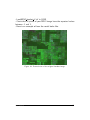
2. Run oft-shptif.bash:
o f t −s h p t i f . b a s h s h a p e f i l e / l a n d u s e . shp i m a g e s / l a n d s a t t 1 . t i f
r e s u l t s / raster landuse . t i f landuse
User Manual
63
3. Open the output results/raster landuse.tif in QGIS, or use it for
further calculations. For all areas without landuse information in
the shapefile, value 0 will be recorded in the output image.
User Manual
64
7.21
oft-sigshp.bash
NAME
oft-sigshp.bash - creates a signature file of an image based on training area polygons.
OFGT VERSION
1.25.4
SYNOPSIS
- oft-sigshp.bash
- oft-sigshp.bash <image><shapefile basename><shapefile id fieldname>
<shapefile coverclass fieldname><output sigfile>
- oft-sigshp.bash <image><shapefile basename><shapefile id fieldname>
<shapefile coverclass fieldname><output sigfile><image projection EPSG>
<shp projection EPSG>
DESCRIPTION
oft-sigshp.bash creates a signature file of an image, e.g. Landsat,
based on training area polygons in shapefile format. This file can
be used in knn-classification with stand alone program oft-nn.
NOTE: do not put .shp into the second parameter (basename)!
- The training areas and the image must be in the same projection
OR you may give the projections in the command line as EPSG
codes.
- If the projections are not defined (for both or one of the inputs),
or the program does not recognize it, the script will warn. This is
not dangerous if the files really are similarly aligned.
- The ID’s must fit into a 16-bit Unsigned image ( 65500).
- The class values may be either numerical or verbal (e.g. ”bushland”)
Minimum parameters needed:
1 = imagefile
2 = shapefile
User Manual
65
3 = f i e l d name s t o r i n g i d s i n s h a p e
4 = f i e l d name s t o r i n g n u m e r i c c l a s s v a l u e s i n s h a p e
5 = ouput s i g n a t u r e f i l e n a m e
OPTIONS
Parameters:
6 = p r o j e c t i o n o f image f i l e
7 = projection of s h a p e f i l e
OTHERS
This script can also be used after oft-nn.
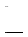
EXAMPLE
- For this exercise following tools are used: oft-sigshp.bash - Open
your working directory using
cd /home / . . .
The script oft-sigshp.bash is able to create a signature file for both
data types, numerical and factorial, depending on the stored data
in your shapefile. In the next steps we will lead you through an
example exercises for each data type:
Figure 11: Attribute table of polyN20.shp.
User Manual
66
1. oft-sigshp.bash creating signature file with numerical
values
- First, we run in the command line oft-sigshp.bash with the input
rasterlandsat t1.tif and your input shapefile landuse.shp. id stands
for the shapefile id fieldname; newcol refers to the shapefile coverclass fieldname. If you look at the attribute table of yourlanduse.shp
you will see that under newcol numerical data is stored. Output:
sig newcol.txt.
Note: the extension .shp of your shapefile is not included in the
command line - only the basename!
- Run in terminal:
o f t −s i g s h p . b a s h l a n d s a t t 1 . t i f l a n d u s e i d n e w c o l s i g n e w c o l . t x t
EPSG : 3 2 6 2 0 EPSG : 3 2 6 2 0
- Lets take a look at the first lines of our output sig newcol.txt:
head s i g n e w c o l . t x t
1 11 5 2 . 0 9 7 3 1 7 2 3 . 6 9 6 4 6 3 2 4 . 9 1 9 7 1 1 4 5 . 3 2 1 7 5 3 6 5 . 4 2 7 7 8 5
129.033459 32.060358
2 22 5 4 . 1 5 7 1 5 9 2 5 . 3 4 8 8 3 2 2 8 . 1 7 6 5 6 1 4 8 . 8 0 5 2 7 8 7 2 . 4 6 8 1 5 8
129.166550 34.397944
4 44 5 3 . 8 6 4 4 1 9 2 5 . 2 3 1 6 4 2 2 7 . 9 3 2 2 4 3 5 1 . 4 1 1 3 6 1 7 1 . 9 5 7 9 7 3
129.559346 33.277298
5 55 5 4 . 3 6 7 8 3 5 2 5 . 7 3 4 6 5 9 2 8 . 4 5 3 1 3 6 5 3 . 7 2 5 8 9 3 7 4 . 1 9 0 1 5 5
130.886716 36.174309
6 66 5 0 . 9 8 7 6 3 3 2 3 . 0 4 4 8 9 2 2 3 . 4 5 2 3 1 2 5 2 . 6 5 5 0 9 1 6 5 . 8 6 1 4 2 6
128.754701 29.121125
7 −9999 5 2 . 9 2 6 0 1 4 2 4 . 3 5 3 2 2 2 2 7 . 2 2 4 3 4 4 4 8 . 1 7 6 6 1 1 7 7 . 2 7 6 8 5 0
132.054893 38.276850
8 88 5 4 . 1 3 3 6 5 2 2 5 . 2 1 4 7 9 7 2 8 . 1 4 0 8 1 1 4 9 . 8 4 2 4 8 2 7 4 . 9 8 5 6 8 0
131.004773 37.408115
9 99 5 4 . 7 7 2 5 1 9 2 5 . 9 6 1 8 3 2 2 9 . 0 3 6 6 4 1 5 2 . 7 8 6 2 6 0 7 8 . 0 3 5 1 1 5
130.658015 39.607634
10 1000 5 1 . 5 8 8 7 2 3 2 3 . 1 3 4 3 2 8 2 4 . 2 5 5 3 9 0 4 5 . 4 8 7 5 6 2 6 8 . 2 0 8 9 5 5
130.310116 33.121061
11 1111 5 3 . 2 3 6 9 4 8 2 4 . 6 4 4 5 7 8 2 7 . 4 2 3 6 9 5 4 8 . 7 7 9 1 1 6 6 8 . 9 4 3 7 7 5
131.594378 33.905622
- The first column refers to the ID, col2 refers to the numerical data
that stored under newcol in the shapefile, Col3 - col9 contain pixel
values of band1 - band7 of the Landsat imagery.
User Manual
67
2. oft-sigshp.bash creating signature file with factorial values
- second, we run the script using the id column called colour, which
stores factorial values. Output: sig colour.txt. Output signature file:
sig colour.txt.
- Run in terminal:
o f t −s i g s h p . b a s h l a n d s a t t 1 . t i f l a n d u s e i d c o l o u r s i g c o l o u r . t x t
EPSG : 3 2 6 2 0 EPSG : 3 2 6 2 0
Again let’s take a closer look at the first lines of the output file
sig colour.txt:
head s i g c o l o u r . t x t
1 red 52.097317 23.696463 24.919711 45.321753 65.427785
129.033459 32.060358
2 green 54.157159 25.348832 28.176561 48.805278 72.468158
129.166550 34.397944
4 orange 53.864419 25.231642 27.932243 51.411361 71.957973
129.559346 33.277298
5 pink 54.367835 25.734659 28.453136 53.725893 74.190155
130.886716 36.174309
6 red 50.987633 23.044892 23.452312 52.655091 65.861426
128.754701 29.121125
7 blue 52.926014 24.353222 27.224344 48.176611 77.276850
132.054893 38.276850
8 orange 54.133652 25.214797 28.140811 49.842482 74.985680
131.004773 37.408115
9 green 54.772519 25.961832 29.036641 52.786260 78.035115
130.658015 39.607634
10 o r a n g e 5 1 . 5 8 8 7 2 3 2 3 . 1 3 4 3 2 8 2 4 . 2 5 5 3 9 0 4 5 . 4 8 7 5 6 2 6 8 . 2 0 8 9 5 5
130.310116 33.121061
11 r e d 5 3 . 2 3 6 9 4 8 2 4 . 6 4 4 5 7 8 2 7 . 4 2 3 6 9 5 4 8 . 7 7 9 1 1 6 6 8 . 9 4 3 7 7 5
131.594378 33.905622
- In comparison to the output of sig newcol.txt we can now see that
col2 of sig colour.txt contains the factorial data.
User Manual
68
7.22
PointsToSquares.py
NAME
PointsToSquares.py - converts XY-locations into 100 x 100 m
squares in a kml-file.
OFGT VERSION
1.25.4
SYNOPSIS
PointsToSquares.py
PointsToSquares.py <infile><outfile><UTM zone number><ID><Xfield><Y-field>
DESCRIPTION
PointsToSquares.py Conversion of user-defined plot centre points
in a text file into squares of 100 x 100 m in kml format. These
squares are training data collection locations, meant to be used with
a specific tool made for Google Earth.
Input textfile projection needs to be UTM South WGS84 zones.
Output kml is in latlon WGS84.
EXAMPLE
- For this exercise following tools are used: PointsToSquares.py,
gdalinfo
• Either use your own .txt file consisting of three columns:
<ID><X-field><Y-field>or
• Generate it by using oft-gengrid.bash
- Open your working directory using
cd /home / . . .
3. In this exercise we use the .txt file derived from oft-gengrid.bash
called training.txt. This is how the first 10 rows look like:
User Manual
69
head t r a i n i n g . t x t
4. NOTE, that the projection is UTM South WGS84 zones. In
our case it is UTM Zone 20S.
5. How to find out? Before running oft-gengrid.bash, check the
projection of the input image (landsat t1.tif ), which is the base to
calculate training.txt using
gdalinfo
l a n d s a t t 1 . t i f // p a r t o f o u t p u t : PROJCS [ ”WGS 84 / UTM
z o n e 20S”
5. After generating training.txt run the command line for calculating
your points to 100 x 100x meter squares, creating an kml outputfile
called Points2Squares training.kml :
P o i n t s T o S q u a r e s . py t r a i n i n g . t x t P o i n t s 2 S q u a r e s t r a i n i n g . kml 20 1
2 3 // 20 r e f e r s t o o u r UTM Zone , n r 1−3 r e f e r t o t h e c o l u m n s
i n our input f i l e t r a i n i n g . t x t
6. Load your result Points2Squares training.kml e.g. in GoogleEarth
7. Check if the individual square is 100 x 100 meter!
User Manual
70
IMAGE MANIPULATION
7.23
multifillerThermal.bash
NAME
multifillerThermal.bash - is a script which utilizes several Landsat
scenes to build a multi-temporal image composite using the warmest
pixel -method.
OFGT VERSION
1.25.4
SYNOPSIS
multifillerThermal.bash
multifillerThermal.bash <anchor><filler1><filler2>... <filler n>
DESCRIPTION
The aim is to have one good image so called anchor with as few
problematic areas as possible and then another which is from same
season (as close a date as possible) and has clouds in different
locations so called filler.
EXAMPLE
- For this exercise following tools are used: multifillerThermal.bash
- Open your working directory using
cd /home / . . .
- Then run
m u l t i f i l l e r T h e r m a l . bash anchor . t i f
User Manual
filler . tif
71
7.24
oft-calc
NAME
oft-calc - is a raster image calculator.
OFGT VERSION
1.25.4
SYNOPSIS oft-calc
oft-calc <input><output>
oft-calc <input><output>[-um maskfile] [-inv] [-of format] [-Z/M/Q/C/L/X/M]
oft-calc <input><output>[-ot Byte/Int16/UInt16/UInt32/Int32/Float32/Float64/
CInt16/CInt32/CFloat32/CFloat64]
DESCRIPTION
oft-calc based on an input raster file, oft-calc creates an output
raster file as result of a simple calculation between the original bands.
The bands used for the calculation must be all stacked in the input
raster file.
After defining the first line, following parameters will be asked:
1. Number of output bands
2. Input postfix equations
Band 1 : The equation for output band 1 has to be specified. The
input bands are referred to with #. The implemented operators
between input bands include:
+
−
/
∗
=
<
>
!
?
M
m
addition
subtraction
division
multiplication
equals to
l e s s than
l a r g e r than
not equal to
i f clause
maximum o f two v a l u e s
minimum o f two v a l u e s
User Manual
72
B
e
c
r
ˆ
e
x
bit l e v e l operator
natural logarithm
p i x e l column c o o r d i n a t e
p i x e l row c o o r d i n a t e
power
natural logarithm
base −e e x p o n e n t i a l f u n c t i o n
OPTION
Parameters:
-inv the notation of the equations has changed in version 2.0. In
case you want to use the old notations, please use the -inv option.
-of format. Any GDAL output format can be specified. If not specified, output format will be tif.
-ot output data type. If not specified, output data type will be the
same as input data type. -[-ot Byte/Int16/UInt16/UInt32/Int32/Float32/Float64]
- output data type
-[Z/M/Q/C/L/X/M] - try to speed up the processing by reading n
lines at the time.
Z=2000 M=1000 Q=500 L=50 X=10
-um mask. If a raster file is provided as a mask, only pixels with
value different than 0 in the mask will be used for the calculation.
NOTE
The notation of the equations has changed in version 2.0. In case
you want to use the old notations, please use the -inv option.
EXAMPLE
For this exercise following tools are used: oft-calc
1. EXAMPLES: OPERATORS
1. Addition
Simple band addition: band1 + band2
o f t −c a l c i n i m a g e o u t i m a g e // h i t r e t u r n a f t e r d e f i n i n g t h i s
line
User Manual
73
2 // t h i s number d e f i n e s t h e number o f bands y o u r o u t i m a g e
w i l l h av e ; h i t r e t u r n a g a i n
#1 #2 + // t y p e y o u r c l a u s e and h i t r e t u r n . Now o u t i m a g e
s h o u l d be i n p r o c e s s !
2. Division
band1 / band2
o f t −c a l c i n i m a g e o u t i m a g e
2
#1 #2 /
3. Equals to
if pixel value of band1 equals 0 then set it to 0, otherwise to 1
o f t −c a l c i n i m a g e o u t i m a g e
1 // i f ( ? ) band1 = 0 (#1 0 =) t h e n 0 o t h e r w i s e 1 ( 1 0 )
#1 0 = 1 0 ?
4. Boolean
You can also use boolean larger than operator to determine if
#1 >#2
o f t −c a l c i n i m a g e o u t i m a g e
2
#1 #2 >
5. The usage of the IF clause
if band1 ¿ 50, output=1 else output=0. This also creates
also a simple mask containing 1 for pixels of interest and 0 for
background
o f t −c a l c i n i m a g e o u t i m a g e
1
#1 50 > 0 1 ?
// i f ( ’ ’ ? ’ ’ ) band1 > 50 ( ’ ’#1 50 > ’ ’) t h e n 1
o t h e r w i s e 0 ( ’ ’ 0 1 ’ ’ ) i f band1 + band2 = 2 , o u t p u t=1
e l s e o u t p u t=0
o f t −c a l c i n i m a g e o u t i m a g e
1
#1 #2 + 2 = 0 1 ? // i f ( ’ ’ ? ’ ’ ) band1 + band2 ( ’ ’#1 #2 + ’ ’)
= 2 ( ’ ’ 2 = ’ ’) t h e n 1 o t h e r w i s e 0 ( ’ ’ 0 1 ’ ’ ) i f band1 > 50
o r band2 > 5 0 , o u t p u t=1 e l s e o u t p u t=0
User Manual
74
o f t −c a l c i n i m a g e o u t i m a g e
1
#1 50 > #2 50 > 0 1 ? 1 ? // i f band1 > 50 ( ’ ’#1 50 > ’ ’)
t h e n 1 ( ’ ’ 1 ? ’ ’ ) o t h e r w i s e i f band2 > 50 ( ’ ’#2 50 > ’ ’)
then 1 o t h e r w i s e 0 ( ’ ’0 1 ? ’ ’)
2. EXAMPLES ON APPLICATIONS
1. NDVI
Calculate the NDVI for your Landsat image (band3 = Red
band, band4 = NIR Band)
o f t −c a l c −o t F l o a t 3 2 i n i m a g e o u t i m a g e
1
#4 #3 − #4 #3 + / // ( b4−b3 ) / ( b4+b3 )
Note that the band4 in the input layerstack image should be
the NIR band and the band 3, the Red band. Note also that
the output data type should be specified as Float32 in order
to have output values from -1 to 1
oft-ndvi.bash also creates a NDVI image using (NIR-VIS) /
(NIR + VIS) .
2. NBR - Normalised Burn Ratio
NBR highlights areas that have burned using Landsat TM.
Calculate the NBR for your Landsat image:
o f t −c a l c i n i m a g e o u t i m a g e
1
#4 #7 − #4 #7 + /
// ( b4−b7 ) / ( b4+b7 )
3. dNBR
In addition, the differnence NBR (dNBR) technique is a form
of Change Detection which is used to index the severity of a
fire
Calculate the differenced (or delta) dNBR for NBR prefire NBR postfire:
Note: as you can’t have two separate input files, one for
User Manual
75
NBR prefire and a second for NBR postfire, you need to combine the two output bands into one file before applying the
equation (band 1 (#1) containing information on NBR prefire
and band 2 (#2) containing info on NBR postfire):
o f t −c a l c i n i m a g e o u t i m a g e
1
#1 #2 −
// band 1 (#1) c o n t a i n s i n f o on N B R p r e f i r e and
band 2 (#2) c o n t a i n s N B R p o s t f i r e
4. Average of bands
Compute an average of bands 1,2 and 3 of an image:
o f t −c a l c i n i m a g e o u t i m a g e
1
#1 #2 + #3 + 3 / // band1 + band 2 (#1 #2 +) + band3 (#3 +)
d i v i d e d by 3 ( 3 / )
5. Build a mask from LEDAPS QA layer
Bit level operators: does the first bit of band 2 equals to 1?
1 #2 B
to build a mask from LEDAPS QA layer:
1 #1 B 0 2 #1 B 4 #1 B + 8 #1 B + 9 #1 B + 12 #1 B + < 2 1 ?
1 ?
which becomes
1 #1 B
0
2 #1 B
4 #1 B
+
8 #1 B
+
9 #1 B
+
12 #1 B
+
<
User Manual
:
:
:
:
:
:
:
:
:
:
:
:
i f b i t one o f band 1 e q u a l s t o 1
constant
i f b i t 2 o f band 1 e q u a l s t o 1
i f b i t 4 o f band 1 e q u a l s t o 1
sum up t h e p r e v i o u s two t e r m s
i f b i t 8 o f band 1 e q u a l s t o 1
sum up p r e v i o u s two t e r m s
i f b i t 9 o f band 1 e q u a l s t o 1
sum up p r e v i o u s two t e r m s
i f b i t 12 o f band 1 e q u a l s t o 1
sum up p r e v i o u s two t e r m s
i f p r e v i o u s term i s s m a l l e r t h a n
76
2
1
?
1
?
:
:
:
:
:
output 2 ( i f c l a u s e f a l s e )
output 1 ( i f c l a u s e true )
if
output 1 ( i f c l a u s e true )
if
Now, what happens in practice, is the following:
1 ) Check b i t 1 and r e c o r d 0 i f i t s i s f a l s e and 1 i f i t i s
true
2 ) Check b i t s 2 , 4 , 8 , 9 and 12 and r e t u r n t h e i r sum
3 ) i f o u t p u t o f 2 ) i s l a r g e r t h a n z e r o ( s e c o n d l i n e a bo ve )
return 1 else return 2
4) i f output of 1) i s 1 return 1 e l s e return output of 3)
6. Creating a mask file
Create a simple mask containing 1 for pixels of interest and 0
for background:
The equation in words: if your pixel value equals 0 then set it
to 0, otherwise to 1
o f t −c a l c i n i m a g e o u t i m a g e
1 // n o t e t h a t h e r e we want t o d e f i n e o u r mask c a l l e d
o u t i m a g e t o c o n s i s t o f 1 band
#1 0 = 1 0 ?
7. Including a mask file
o f t −c a l c −um i n m a s k i n i m a g e o u t i m a g e
// h e r e t h e o p t i o n
−um d e f i n i n g t h e mask f i l e i s added t o t h e command
2
#1 #2 +
User Manual
77
7.25
oft-chdet.bash
NAME
oft-chdet.bash - automated change detection.
OFGT VERSION
1.25.4
SYNOPSIS oft-chdet.bash
oft-chdet.bash <input1><input2><output><nodata value>[threshold]
- <input1>- Input raster 1 (with extension).
- <input2>- Input raster 2 (with extension).
- <output>- A raster consisting of binary values (0 or 1) indicating
pixels of likely change between the two dates. Values of 1 indicate
change. Values of 0 indicate no-change.
- <nodata value>- Value indicating no-data within the image.
- [threshold] - Default 0.99. Specifies the threshold value of the cumulative frequency distribution (of the resulting Chi-square layer...see
Reference below) above which pixels are identified as changed.
Higher threshold values indicate more stringent limits for detecting
changes and, thus, produce less changed area than lower thresholds.
Threshold values must be specified as a proportion using 0.XX notation.
DESCRIPTION
This tool performs automated change detection between 2 input
images. The script uses the Iteratively Re-weighted Multivariate
Alteration Detection (MAD) algorithm (Canty and Nielsen, 2008).
Input imagery must have the same format, extent, resolution, number of bands and type of data.
User Manual
78
REFERENCE
M. J. Canty and A. A. Nielsen (2008), Automatic radiometric normalization of multitemporal satellite imagery with the iteratively
re-weighted MAD transformation RSE 112(3), 1025-1036.
EXAMPLE
To automatically find changes between a landsat image from year
2000 and 2005 using a threshold of 0.85:
o f t −c h d e t . b a s h l a n d s a t 0 0 . t i f l a n d s a t 0 5 . t i f c h a n g e 0 0 0 5 . t i f 0
0.85
EXERCISE
- For this exercise following tools are used: oft-chdet.bash
- Identify changed areas between year 2000 and 2012 using Landsat
imagery using landsat t1.tif and landsat t2.tif
1. Open your working directory using
cd /home / . . .
2. Unpack the data
3. Now we run oft-chdet.bash to do the automated change detection
using the input Landsat data
o f t −c h d e t . b a s h l a n d s a t t 1 . t i f l a n d s a t t 2 . t i f c h a n g e 0 0 1 2 . t i f 0
0.85
Output includes the following:
A file beginning with imad-[name of outfile].tif. This file contains
the raw results of the IMAD process, one for each input band and
the chi-squared layer (see Reference).
The specified output file:
This file contains 1’s and 0’s; 1’s indicate areas of change and 0’s
indicate areas of no change.
User Manual
79
7.26
oft-clip.pl
NAME
oft-clip.pl - subsets an input image using the extent, pixels size and
projection of a reference image.
OFGT VERSION
1.25.4
SYNOPSIS oft-clip.pl
oft-clip.pl <reference><input><output>
DESCRIPTION
oft-clip.pl The straight forward tool oft-clip.pl subsets an input
image using the extension, pixel size and projection of the reference
image.
EXERCISE
-For this exercise following tools are used: oft-clip.pl
1. Use for this exercise the MODIS imagery vcf-2010.tif and the
Landsat imagery clip landsat t1.tif
2. Open your working directory using
cd /home / . . . / OFGT−Data
3. Reproject, clip and resample the MODIS image (resolution 230
m, lat/long) to the projection, extent and pixel size of the Landsat
tile (resolution 30m, UTM 35)
o f t − c l i p . p l i m a g e s / l a n d s a t . t i f i m a g e s / v c f −2010. t i f
clip . tif
r e s u l t s / vcf−
4. Visualize the results in QGIS
q g i s images / l a n d s a t t 1 . t i f
User Manual
r e s u l t s / vcf −c l i p . t i f
80
7.27
oft-combine-images.bash
NAME
oft-combine-images.bash - combines 2 images into one.
OFGT VERSION
1.25.4
SYNOPSIS oft-combine-images.bash
oft-combine-images.bash <-a first image><-b second image><-m
first image mask><-s second mask>
-a First image = Better image, whose area is used whenever possible
-b Second image = Image to be used elsewhere
-m First image mask = 0/1 mask indicating bad areas on first image
with 0
-s Second mask = 0/1 mask indicating bad areas on second image
with 0
DESCRIPTION
- Can be used to merge same-day Landsat images (adjacent) or two
gapfill results (stack)
- Takes as input the images and their masks
- Masks for same-day can be prepared with oft-trim-mask.bash and
for gapfill with oft-prepare-images-for-gapfill.bash
- All ok areas are taken from image 1, and image 2 is used elsewhere
- Also produces a mask that indicates ok areas of the resulting
combined image with 1
- All material needs to be in same projection
- Works with 6 or 7 band images
EXERCISE
- For this exercise following tools are used: oft-combine-images.bash,
gdal translate, trim
User Manual
81
- Open your working directory using
cd /home / . . . / OFGT−Data
- In a first step we need to adjust the nr of bands of landsat t1.tif
(7 bands) to the nr of bands of our second image (6 bands):
g d a l t r a n s l a t e l a n d s a t t 1 . t i f l a n d s a t t 1 6 b a n d s . t i f −b 1 −b 2 −b
3 −b 4 −b 5 −b 6
- Then we need to prepare our mask files for each landsat image
using oft-trim
o f t −t r i m −mask . b a s h l a n d s a t t 2 . t i f
o f t −t r i m −mask . b a s h l a n d s a t t 1 . t i f
Now we can run oft-combine-images.bash. The output is automatically processed, in this case it is called stack landsat t1 6bands landsat t2.tif
o f t −combine−i m a g e s . b a s h −a l a n d s a t t 1 6 b a n d s . t i f −b l a n d s a t t 2
. t i f −m l a n d s a t t 1 m a s k . t i f −s l a n d s a t t 2 m a s k . t i f
User Manual
82
7.28
oft-gapfill
NAME
oft-gapfill - regression based gap and cloud filler.
OFGT VERSION
1.25.4
SYNOPSIS oft-gapfill
oft-gapfill <-um maskfile><input><output>
oft-gapfill <-um maskfile><input><output>[-la nbrLargeAreaWindows] [-nolocal] [-smooth] [-pm] [-da] [-sd sampling density] [-ws
WindowSize]
DESCRIPTION
oft-gapfill fills the gaps in an input image using locally built regression models. The models can be built
1. separately for every gap pixel using a local model built using its
adjacent pixels or
2. for a given number of Large Area subsets or
3. using both of these methods
- In the case 2), the option -la followed by the number of requested
Large Area (LA) subsets in X direction should be given. The total
number of LA subsets is the square of the given parameter. If the
user wants to use only Large Area models, the option -nolocal should
be used.
- Maskfile, inputfile and outputfile are all required inputs. They may
be in any of the formats understood by GDAL.
- The input image is a stack of the Anchor image and the Filler
image. The output values for Anchor are computed using Filler and
the model. The input image bands should be organized as follows:
User Manual
83
• band 1 to nbr bands/2 = Anchor image
• bands nbr bands/2 + 1 to nbr bands = Filler image
- The mask file shows the locations of the gaps, areas which are
suitable for collecting training data, and areas which should not be
processed. The mask values are as follows:
1 = f i l l t h e s e p i x e l s ( u n u s a b l e d a t a i n a nc h o r , good d a t a i n
filler )
2 = c o l l e c t t r a i n i n g d a t a f o r r e g r e s s i o n model ( good d a t a i n
both images )
3 = do n o t h i n g , i . e . , u s e t h e o r i g i n a l v a l u e s ( 2 c a s e s : good i n
a n c h o r , bad i n f i l l e r OR non−good i n b o t h i m a g e s )
0 = do n o t h i n g ( image m a r g i n s )
OPTIONS
1. -la (nbrLargeAreaWindows) = number of LA windows in X direction. The total number of LA windows will be the square of this
parameter.
2. -da (do4allpixels) = use to built model to predict output value
for every pixel of the anchor using the built models and the values
of the Filler.
3. -sd (sampling density) = sampling density used to build the
LargeArea model. Value two, for example, would force the algorithm
to collect every other valid pixel within the scene to be used in
building the model.
4. -ws (WindowSize) = size of the neighbourhood from which the
data for local model construction is collected
NOTE
The input image can be produced from 2 image stacks (for instance, 2 Erdas imagine composites consisting of 7 bands). The
script stack2images.bash produces the composite. It can also be
produced from HDF-images that are stored in folders. The script
stack2images hdf.bash is for that purpose.
User Manual
84
The model may be very sensitive to outliers. Therefore it is important that the mask value 2 is present only in location where both
Anchor and Filler have valid data.
IMPORTANT: The stack and the mask must have been
reprojected to the same geographical window and they do
must have the same number of rows and cols
EXAMPLE
o f t − g a p f i l l − l a 2 − n o l o c a l −s d 5 −ws 13 −um mymask . img
my14bandimage . img f i l l e d . img
The program performs 2 passes over the image:
- Pass1: collect the data to build the model
- Pass2: fill the gaps with Large Area models.
EXERCISE
- For this exercise following tools are used: oft-gapfill, gdal translate,
oft-stack, oft-calc
- Open your working directory using
cd /home / . . .
- As oft-gapfill only allows even number of bands, first, we need to
adjust the number of bands of landsat t1.tif (7 bands) landsat t2.tif
(6 bands):
g d a l t r a n s l a t e l a n d s a t t 1 . t i f l a n d s a t t 1 6 b a n d s . t i f −b 1 −b 2 −b
3 −b 4 −b 5 −b 6
- oft-gapfill takes as input an image stack of the anchor (landsat t2.tif )
and the filler (landsat t1.tif ):
o f t −s t a c k −o s t a c k . t i f l a n d s a t t 2 . t i f l a n d s a t t 1 6 b a n d s . t i f
- Gapfilling with mask of the scan-line using a simple mask created
with oft-calc in two steps:
Rules:
User Manual
85
• if band 1 or band 6 are 0 put 1 (fill)
• if band 7 or band 12 are 0 put 3 (do nothing)
• else put 2 (collect training data for regression models)
Step 1:
o f t −c a l c s t a c k . t i f tmp . t i f
Step 2 :
#1 0 = #6 0 = + 0 > 2 1 ?
#7 0 = #12 0 = + 0 > 2 3 ?
Step 2:
o f t −c a l c s t a c k . t i f tmp . t i f
Step 2 :
#1 0 = #6 0 = + 0 > 2 1 ?
#7 0 = #12 0 = + 0 > 2 3 ?
Now, use oft-gapfill to fill the areas indicated as ”1” in the mask:
o f t − g a p f i l l − l a 1 − n o l o c a l −pm −s d 2 −um s i m p l e m a s k . t i f s t a c k .
tif filled la1 sd2 simplemask . tif
Output automatically processed: filled la1 sd2 simplemask.tif
Figure 12: Original Landsat image.
User Manual
86
Figure 13: Landsat imager after gap fill
User Manual
87
7.29
oft-ndvi.bash
NAME
oft-ndvi.bash - computes ndvi images.
OFGT VERSION
1.25.4
SYNOPSIS oft-ndvi.bash
oft-ndvi.bash <input><output><R band><NIR band>
<input><output><R band><NIR band>[mask]
DESCRIPTION
oft-ndvi.bash creates an NDVI image using (NIR-VIS) / (NIR +
VIS).
- Input data is an image stack. User gives the location of Red and
NIR band (in regular Landsat TM/ETM 3 and 4)
- Number of bands is not restricted
OPTIONS
- [mask] - include a mask image into this process by using this option
EXAMPLE
- For this exercise following tools are used: oft-ndvi.bash
- Open your working directory using
cd /home / . . .
- Run the command line for calculating the NDVI for your satellite image where landsat t1.tif is your input image and NDVI landsat t1.tif
will be your NDVI output image. The numbers <3>and <4>refer
to the band numbers for the VIS and NIR bands.
o f t −n d v i . b a s h l a n d s a t t 1 . t i f
User Manual
. . / r e s u l t s / NDVI landsat t1 . t i f 3 4
88
- LoadNDVI landsat t1.tif in QGIS
- Check that all pixels of your NDVI image have the expected values
between -1 and 1.
- Here is an example of how the result looks like:
Figure 14: Zoomed view of the original Landsat image.
User Manual
89
Figure 15: Zoomed view of the NDVI-result using the ’freak out’ colour map in
QGIS.
User Manual
90
7.30
oft-prepare-images-for-gapfill.bash
NAME
oft-prepare-images-for-gapfill.bash - prepares images and masks for
oft-gapfill
OFGT VERSION
1.25.4
SYNOPSIS oft-prepare-images-for-gapfill.bash
oft-prepare-images-for-gapfill.bash <-a anchor><-f filler><-m anchor mask><-s second mask (filler)>
oft-prepare-images-for-gapfill.bash <-a anchor><-f filler><-m anchor mask><-s second mask (filler)>[-n ndvi threshold]
-a Anchor = Better image, whose gaps are to be filled
-f Filler = Filler image
-m Anchor mask = 0/1 mask indicating bad areas on anchor image
with 0
-s Second mask = 0/1 mask indicating bad areas on filler image
with 0
OPTIONS
-n ndvi threshold = If images differ a lot, NDVI can be used to select
only vegetated areas for mask
Values like 0.4 or 0.5 are useful at some location on the world, check
your particular situation yourself!
DESCRIPTION
oft-prepare-images-for-gapfill.bash
- Takes the anchor and filler images as input
- Also their 0/1 masks indicating clouds and gaps are needed
- NDVI can be used to threshold areas with low vegetation off from
User Manual
91
the models
- At this point, bands 3 and 4 are used for NDVI computation
- Otherwise, nbr of bands is not fixed, but must be equal in the
input images
- All material needs to be in same projection
EXAMPLE
- For this exercise following tools are used: oft-prepare-images-forgapfill.bash
- Open your working directory using
cd /home / . . .
- As landsat t1.tif and landsat t2.tif differ in their number of bands
we need to exclude band 7 from landsat t1.tif by carrying out
following procedure:
g d a l t r a n s l a t e l a n d s a t t 1 . t i f l a n d s a t t 1 6 b a n d s . t i f −b 1 −b 2 −b
3 −b 4 −b 5 −b 6
Let’s run oft-prepare-images-for-gapfill.bash using following input:
o f t −p r e p a r e −images −f o r − g a p f i l l . b a s h −a l a n d s a t t 1 6 b a n d s . t i f −f
l a n d s a t t 2 . t i f −m l a n d s a t t 1 m a s k . t i f −s l a n d s a t t 2 m a s k . t i f
Two output images mask are automatically processed: gapmask landsat t1 6bands land
and goodarea mask landsat t1 6bands landsat t2.tif
Figure 16: gapmask landsat t1 6bands landsat t2.tif
User Manual
92
Figure 17: goodarea mask landsat t1 6bands landsat t2.tif
User Manual
93
7.31
oft-reclass
NAME
oft-reclass - is a reclassification program.
OFGT VERSION
1.25.4
SYNOPSIS
oft-reclass
oft-reclass <inpufile>
oft-reclass [OPTIONS] <inpufile>
DESCRIPTION
oft-reclass changes pixel values to alterenative values given in a text
file .
The maxval parameter is used to allocate memory for the reclassification table. If it is not given in the command line, it will be asked
interactively.
The reclassification text file should consist of records with input
value (column 1) and one or more space separated output values.
Thus, the structure could be:
1
2
3
4
255
0 0
125
0 0
255 255
0
100 16
112
The program asks, how many output values the user wants to
produce for each input band. With the given example reclassification
file, the user could produce a 3 band RGB image from a single band
input file.
OPTIONS
−um
<m a s k f i l e >
User Manual
94
−o i <o u t p u t i m a g e >
−maxval <maximum p i x e l v a l u e i n i n f i l e >
EXAMPLE
- For this exercise following tools are used: oft-reclass
- For this exercise we use a single band image images/forestc.tif and
a segmented image images/segments.tif which you can also create
yourself using oft-seg.
- Open your working directory using
cd /home / . . .
1. oft-reclass
- First you need to create a text file called input reclass.txt that
should look like this:
1 255 255 255
2 0 100 0
3 125 100 16
4 0 0 112
5 0 225 0
6 225 0 0
99 200 0 200
- Now we run oft-reclass with Input: image/forestc.tif and text/input reclass.txt;
Output: results/reclassforestc.img :
o f t −r e c l a s s −o i r e s u l t s / r e c l a s s f o r e s t c . img
t x t images / f o r e s t c . t i f
txt / input reclass .
- Then tool will ask you then for further information:
I n p u t r e c l a s s f i l e name ? : t x t / i n p u t r e c l a s s . t x t
Nbr o f o u t bands p e r i n p u t c h a n n e l ? : 3
Col of i n p u t v a l u e ? : 1
Col of output v a l u e 1 : 2
Col of output v a l u e 2 : 3
Col of output v a l u e 3 : 4
NODATA v a l u e ? : 0
- Open QGIS and load your the original imagery image/forestc.tif
(Colour map: Pseudocolour) and the result results/reclassforestc.img.
Click with the Identify Features Tool over the the different classes
and see how they have changed after the reclassification:
User Manual
95
Figure 18: Original input image forestc.tif.
Figure 19: Reclassified output raster reclassforestc.img.
User Manual
96
2. Second example for oft-reclass
- Lets run oft-reclass again with a different input image: Input:
landsat t1 min50.tif, input reclass.txt, input reclass.txt; Output:
reclass min50.img:
o f t −r e c l a s s −o i r e c l a s s m i n 5 0 . img
txtlandsat t1 min50 . t i f
input reclass .
Again the tool will ask you for further information:
I n p u t r e c l a s s f i l e name ? : i n p u t r e c l a s s . t x t
Nbr o f o u t bands p e r i n p u t c h a n n e l ? : 3
Col of i n p u t v a l u e ? : 1
Col of output v a l u e 1 : 2
Col of output v a l u e 2 : 3
Col of output v a l u e 3 : 4
NODATA v a l u e ? : 0
- Open QGIS and load your result image reclass min50.img and zoom
into the top left corner. You can see that the original classes 1-6
and 99 of landsat t1 min50.tif were reclassified the way we defined
it in the lookup table input reclass.txt.
User Manual
97
Figure 20: Zoom into the top left corner of our final result reclass min50.img.
User Manual
98
7.32
oft-shrink
NAME
oft-shrink - to be combined with oft-trim.
7.33
oft-stack
NAME
oft-stack - Create a muti-band image stack.
OFGT VERSION
1.25.4
SYNOPSIS
oft-stack
oft-stack <-o outputfile><inputfiles>
oft-stack [-ot Byte/Int16/UInt16/UInt32/Int32/Float32/Float64/CInt16/CInt32/
CFloat32/CFloat64] [-um <maskfile>] <-o outputfile><inputfiles>
−o o u t p u t f i l e − The name o f t h e o u t p u t f i l e t o be c r e a t e d (
include extension ) .
i n p u t f i l e s − A s e t of i n p u t f i l e s ( i n c l u d e e x t e n s i o n ) , each
s e p a r a t e d by a s p a c e .
DESCRIPTION
oft-stack builds image stack from input files in the order of appearance.
- The output format of the first input file is used.
- The images need to have exactly the same size (rows x cols)
OPTIONS
−o t − O p t i o n a l . The o u t p u t image t y p e . By d e f a u l t , t h e f i r s t
i n p u t image t y p e i s u s e d .
User Manual
99
−um − O p t i o n a l . A mask f i l e u s e d t o r e s t r i c t t h e e x t e n t o f t h e
processing .
- oft-stack builds an image stack from input files in the order of
appearance. By default, the output format and type of the first
input file is used.
- N.B.: The images need to have exactly the same size (rows x cols)
EXAMPLE
To create a 6-band stack of Landsat data from individual input
rasters in .TIF format.
o f t −s t a c k −o l a n d s a t 7 b a n d . t i f l a n d s a t b 1 . t i f l a n d s a t b 2 . t i f
landsatb3 . t i f landsatb4 . t i f landsatb5 . t i f landsatb7 . t i f
the above can be written using wildcards...
o f t −s t a c k −o l a n d s a t 7 b a n d . t i f l a n d s a t ∗ . t i f
EXERCISE
For this exercise following tools are used: oft-stack
1. Open your working directory using
cd /home / . . .
2. Now we run oft-stack using two input images landsat t1.tif and
landsat t2.tif to create the output stack image called stack.tif :
o f t −s t a c k −o s t a c k . t i f l a n d s a t t 1 . t i f l a n d s a t t 2 . t i f
3. Take a closer look at your output in QGIS and you will see
that stack.tif has 13 bands (landsat t1.tif contains 7 bands and
landsat t2.tif 6 bands). Or print the raster information on your
screen by typing in your terminal
gdalinfo stack . t i f
User Manual
100
7.34
oft-trim
NAME
oft-trim - erosion filter producing binary output.
OFGT VERSION
1.25.4
SYNOPSIS
oft-trim
oft-trim -um <maskfile><inputfile><outfile>
oft-trim [-ws WindowSize] [-origval] -um <maskfile><inputfile><outfile>
DESCRIPTION
oft-trim analyses the content of the spatial neighbourhood of each
pixel. If all the pixels within the window are less or equal to zero,
output is zero. Else, output is one.
OPTIONS
Parameter:
-um = maskfile
-ws = window size
-origval = original value
EXERCISE
For this exercise following tools are used: oft-trim
1. Open your working directory using
cd /home / . . .
2. Lets run oft-trim with the input file landsat t1.tif with the option
-ws set to 3 to create the output file trim.tif :
o f t −t r i m
User Manual
−ws 3 l a n d s a t t 1 . t i f t r i m . t i f
101
3. Verify in QGIS that all the values of your output image are all
trimmed to 1.
User Manual
102
7.35
oft-trim-maks.bash
NAME
oft-trim-maks.bash - This script makes a 0/1 mask of a 6 or 7 band
(Landsat) image .
OFGT VERSION
1.25.4
SYNOPSIS
oft-trim-maks.bash
oft-trim-maks.bash <image>
DESCRIPTION
oft-trim-maks.bash
- detects the margins and Landsat 7 missing scanlines, and trims
the edges
- accepts 6 or 7 band image
- all values ¡= 0 are considered nodata
- Note: the output of oft-trim-maks.bash can be furhter used for
oft-combine-images.bash
EXERCISE
For this exercise following tools are used: oft-trim-mask.bash
1. Open your working directory using
cd /home / . . .
2. Lets run oft-trim-mask.bash using landsat t2.tif. Automatically
processed output: landsat t2 mask.tif :
o f t −t r i m −mask . b a s h l a n d s a t t 2 . t i f
3. Verify in QGIS your our result if the mask pixel values are 1 or 0.
User Manual
103
Figure 21: Original image landsat t2.tif with visible gaps in QGIS
User Manual
104
Figure 22: Output landsat t2 mask.tif using the Pseudo-colour colour map in
QGIS
User Manual
105
STATISTICS
7.36
oft-ascstat.awk
NAME
oft-ascstat.awk - computes basic statistics for a space separated
text file.
OFGT VERSION
1.25.4
SYNOPSIS oft-ascstat.awk
oft-ascstat.awk <input file
textgreater
DESCRIPTION
oft-ascstat.awk computes basic statistics for a given input file or
stdin.
Please not that the data must be provided as space separated!
EXAMPLE
1.For this exercise following tools are used: oft-ascstat.awk
2. Open your working directory using
cd /home / . . .
3. The script oft-ascstat.awk computes basic statistics for our
space separate input file sample landuse.txt:
head s a m p l e l a n d u s e . t x t
10557.00
81.00
94788.00
65.00
7 7 2 6 5 0 . 0 0 −2404770.00 5 . 0 0 5 3 . 0 0 2 6 . 0 0 2 8 . 0 0 5 4 . 0 0
131.00 39.00
7 7 3 4 9 0 . 0 0 −2431680.00 1 . 0 0 5 1 . 0 0 2 4 . 0 0 2 5 . 0 0 4 5 . 0 0
127.00 33.00
User Manual
106
2 0 1 5 3 6 . 0 0 7 7 4 7 5 0 . 0 0 −2439390.00 1 . 0 0 5 4 . 0 0 2 5 . 0 0 2 7 . 0 0 5 0 . 0 0
71.00 130.00 35.00
8 8 5 3 1 . 0 0 7 7 1 4 5 0 . 0 0 −2431110.00 1 . 0 0 4 7 . 0 0 2 1 . 0 0 1 8 . 0 0 3 7 . 0 0
48.00 126.00 21.00
1 2 3 3 7 4 . 0 0 7 7 4 1 5 0 . 0 0 −2433990.00 1 . 0 0 5 4 . 0 0 2 4 . 0 0 3 0 . 0 0 3 5 . 0 0
75.00 132.00 42.00
9 7 3 4 5 . 0 0 7 7 6 2 2 0 . 0 0 −2431950.00 1 . 0 0 5 2 . 0 0 2 3 . 0 0 2 4 . 0 0 4 2 . 0 0
60.00 131.00 30.00
1 9 9 0 4 1 . 0 0 7 7 3 1 9 0 . 0 0 −2439120.00 1 . 0 0 5 1 . 0 0 2 3 . 0 0 2 3 . 0 0 5 2 . 0 0
58.00 130.00 28.00
1 4 4 2 7 6 . 0 0 7 7 5 8 6 0 . 0 0 −2435400.00 1 . 0 0 4 9 . 0 0 2 2 . 0 0 2 1 . 0 0 4 5 . 0 0
59.00 125.00 30.00
1 8 0 9 6 1 . 0 0 7 7 2 6 8 0 . 0 0 −2437890.00 1 . 0 0 4 9 . 0 0 2 1 . 0 0 2 1 . 0 0 3 6 . 0 0
61.00 126.00 28.00
1 8 5 3 8 6 . 0 0 7 7 2 4 1 0 . 0 0 −2438190.00 1 . 0 0 4 9 . 0 0 2 1 . 0 0 1 8 . 0 0 4 3 . 0 0
51.00 126.00 22.00
Explanation of the columns: pixel id x y class band1 band2 band3
band4 band5 band6 band7
4. Lets run oft-ascstat.awk
o f t −a s c s t a t . awk s a m p l e l a n d u s e . t x t
Result is printed on screen:
Col
Min
1
4923
2
736440
3
−2448000
4
1.0
5
44.00
6
19.0
7
16.0
8
34.0
9
42.0
10 1 2 4 . 0
Max
220664.0
787020.0
−2403090
25.0
69.0
37.0
48.0
62.0
103.0
136.0
Avg
116318.43
771921.0
−2431097.6
2.844444
53.455556
24.82
27.02
46.74
69.455
129.43
Std
6345.83
798.10
1035.67
0.519269
0.491606
0.383203
0.691350
0.711611
1.450889
0.252272
Explanation of the columns same as before: pixel id x y class band1
band2 band3 band4 band5 band6 band7
And of course the interesting lines are line 4-11.
User Manual
107
7.37
oft-avg
NAME
oft-avg - computes zone/segment averages and standard deviations.
OFGT VERSION
1.25.4
SYNOPSIS oft-avg
oft-avg -i <input>-o <output>-um <maskfile>
oft-avg -i <input>-o <output>-um <maskfile>[-std]
oft-avg -i <input>-o <output>[-ot Byte/Int16/UInt16/UInt32/Int32
/Float32/Float64] [-h help]
DESCRIPTION
- oft-avg computes zone/segment averages and standard deviations.
- It produces two output files: an output image and a text file.
- You need to give at least the input image file (-i option), the output
image (-o) and the maskfile (-um).
- In the output image, each pixel gets assigned the average/standard
deviation for the zone/segment it belonged to.
- The output format in the text file is: ID number pixels avgband1
...avgbandN.
OPTION
Parameters:
[-std] - The program computes and prints out also the std’s (as
extra bands in the output image and extra columns in the text file)
[-ot Byte/Int16/UInt16/UInt32/Int32/Float32/Float64] - output
data type
[-h help]
User Manual
108
NOTE
For the benefit of users that are running scripts using the older
version based on order of datafiles instead of options -i, -o and -um,
the program can still be used that way
EXAMPLE
For this exercise following tools are used: oft-avg
1. Open your working directory using
cd /home / . . .
2. Now we run oft-avg with input: images/landsat t1.tif, output:
results/oftavg.tif, mask: images/segments.tif
The output text file will be named as the output image plus ”.txt”
(in this case oftavg.tif.txt).
o f t −avg − i i m a g e s / l a n d s a t t 1 . t i f −o r e s u l t s / o f t a v g . t i f −um
images / segments . t i f
3. Print the first 10 lines of the output text file in terminal:
head r e s u l t s / o f t a v g . t i f . t x t
1 135 4 9 . 0 5 1 8 5 2 2 0 . 0 8 1 4 8 1 1 8 . 3 7 0 3 7 0 3 6 . 7 8 5 1 8 5 4 6 . 6 7 4 0 7 4
126.059259 20.192593
2 54 4 9 . 3 5 1 8 5 2 2 0 . 3 7 0 3 7 0 1 8 . 4 0 7 4 0 7 3 7 . 5 0 0 0 0 0 4 6 . 5 5 5 5 5 6
125.925926 19.870370
3 76 4 8 . 5 7 8 9 4 7 1 9 . 8 2 8 9 4 7 1 7 . 7 1 0 5 2 6 3 6 . 6 5 7 8 9 5 4 3 . 8 8 1 5 7 9
125.907895 18.881579
4 194 4 9 . 0 0 5 1 5 5 2 0 . 0 7 7 3 2 0 1 8 . 2 6 8 0 4 1 3 7 . 5 3 0 9 2 8 4 6 . 0 0 0 0 0 0
125.670103 19.721649
5 221 4 9 . 0 9 0 4 9 8 2 0 . 1 7 6 4 7 1 1 8 . 5 7 4 6 6 1 3 7 . 5 4 2 9 8 6 4 7 . 5 6 5 6 1 1
125.728507 20.339367
6 82 4 8 . 8 7 8 0 4 9 2 0 . 3 0 4 8 7 8 1 8 . 6 9 5 1 2 2 3 7 . 2 4 3 9 0 2 4 8 . 0 9 7 5 6 1
125.597561 20.780488
7 53 4 8 . 8 8 6 7 9 2 2 0 . 0 5 6 6 0 4 1 8 . 3 3 9 6 2 3 3 7 . 2 0 7 5 4 7 4 5 . 6 9 8 1 1 3
125.698113 19.396226
8 120 4 8 . 9 9 1 6 6 7 2 0 . 2 1 6 6 6 7 1 8 . 5 8 3 3 3 3 3 6 . 9 0 8 3 3 3 4 7 . 2 0 0 0 0 0
126.041667 20.283333
9 154 4 8 . 9 8 0 5 1 9 1 9 . 9 9 3 5 0 6 1 8 . 3 8 9 6 1 0 3 2 . 4 7 4 0 2 6 4 5 . 0 0 0 0 0 0
125.987013 20.337662
10 150 4 9 . 5 4 0 0 0 0 2 0 . 2 2 0 0 0 0 1 8 . 8 5 3 3 3 3 3 2 . 2 6 0 0 0 0 4 7 . 2 3 3 3 3 3
125.973333 21.433333
User Manual
109
Explanation of values for each column:
- Col1: ID (value for zone/segment)
- Col2: Number of pixels
- Col3 - col9: Average value of band1, band2, ... band7
4. Open the output file results/oftavg.tif in QGIS. Use Identify
Features that can be chosen form the top bar and click on the
image. The window Identify Results should pop up and with the
average value for each band for that zone/segment:
Band1 49
Band2 21
Band3 20
Band4 41
Band5 50
Band6 126
Band7 22
5. If you also choose to output standard deviations, the format of
the output files will be as follows:
- text file:
• Col1: ID (value for zone/segment)
• Col2: Number of pixels
• Col3 - col9: Average value of band1, band2, ... band7
• Col10 - col16: Standard deviation of band1, band2, ... band7
- raster image file:
• band1 - band7: average for band1, band2, ... band7
• band8 - band14: standard deviation for band1, band2, ... band7
User Manual
110
7.38
oft-countpix.pl
NAME
oft-countpix.pl - counts number of pixel with, below or above a
specific value.
OFGT VERSION
1.25.4
SYNOPSIS oft-countpix.pl
oft-countpix.pl <input><value>[-b/-v/-a [band]]
<input>is a raster image
<value>is an real number. If not precised, oft-countpix.pl gives the
total number of pixels. If value is below the min or above the max
of the image, a warning is given
OPTION
-v = count all pixels with value value (default)
-b = count all pixels below value
-a = count all pixels above value
[band] = number of the band. Default is Band 1
DESCRIPTION
oft-countpix.pl counts the number of pixels within an image with
(default), below or above (options) a specific value .
EXAMPLE
For this exercise following tools are used: oft-avg
Open your working directory using
cd /home / . . .
User Manual
111
Usage of oft-countpix.pl using the input image forestc.tif with
pixel value of 33
f t −c o u n t p i x . p l i m a g e s / f o r e s t c . t i f 33
o f t −c o u n t p i x . p l i m a g e s / f o r e s t c . t i f 33 −a
Usage of oft-countpix.pl using the input image landsat t1.tif with
value 50, counting all pixels below, in band 4
o f t −c o u n t p i x . p l i m a g e s / l a n d s a t t 1 . t i f 50 −b 4
User Manual
112
7.39
oft-crossvalidate
NAME
oft-crossvalidate - computes RMSE and bias estimates for k-nn via
leave-one-out cross-validation.
OFGT VERSION
1.25.4
SYNOPSIS oft-crossvalidate
oft-crossvalidate <-i datafile><-k val><-v col><-bands val>
oft-crossvalidate <-i datafile><-k val><-v col><-bands val>[-dw
{1/2/3}] [-x col] [-y col] [-id col] [-norm] [-mindist val] [-maxdist
val] [-dem col thres] [-lu col]
DESCRIPTION
oft-crossvalidate is a Program for carrying out a leave-one-out crossvalidation using nearest neighbour estimation.
- You need to give at least the datafile, number of neighbours (k),
the column for your variable and nbr of bands.
- Bands must be located after all other variables.
- Program is terminated if the spatial neighbourhood restriction
leaves too few (less than k) potential neighbours
- A possible order of data is: id, variable, x-coordinate, y-coordinate,
feature1...featureN.
- Values must be separated with a space or tab.
- Prints the average, RMSE and bias on screen.
- Saves original value, estimate and difference in an output file. If id
or x and y are given, they are printed out as well.
- If the id is indicated in the command line, the id’s of 10 nearest
neighbours are printed into the output file.
User Manual
113
OPTION
Parameters:
- [-dw] - weight the nearest neighbour data with 1=equal (default),
2=inverse distance, 3=squared inv. distance weights.
- [-x] - column for x-coordinate
- [-y] - column for y-coordinate
- [-id] - column for id
- [-norm] - normalize the image features (default is no normalization
- [-mindist] - use a minimum spatial distance (e.g. 1000). Observations closer than that, based on the x and y-coordinates are not
allowed as neighbours (default is no restriction)
- [-maxdist] - use a maximum spatial distance (e.g. 50000). Observations outside that radius are not allowed as neighbours (default is
no restriction)
- [-dem] - column and threshold value (e.g. 1000) for restriction of
neighbours in vertical direction (default is no restriction)
- [-lu] - column used for stratification of the data. If given, separate
RMSEs are computed for each class indicated in the column (default
is no stratification)
EXAMPLE
1. Input data: download for this exercise sample landuse.txt.
You might have created it already in exercise oft-sample-withinpolys.bash.
2. Open your working directory using
cd /home / . . .
3. The script oft-crossvalidate prints the average, RMSE and bias
on screen using the input data file sample landuse.txt. Lets take a
closer look at the input file (space or tab separate):
head s a m p l e l a n d u s e . t x t
User Manual
114
1 0 5 5 7 . 0 0 7 7 2 6 5 0 . 0 0 −2404770.00 5 . 0 0 5 3 . 0 0 2 6 . 0 0 2 8 . 0 0 5 4 . 0 0
81.00 131.00 39.00
9 4 7 8 8 . 0 0 7 7 3 4 9 0 . 0 0 −2431680.00 1 . 0 0 5 1 . 0 0 2 4 . 0 0 2 5 . 0 0 4 5 . 0 0
65.00 127.00 33.00
2 0 1 5 3 6 . 0 0 7 7 4 7 5 0 . 0 0 −2439390.00 1 . 0 0 5 4 . 0 0 2 5 . 0 0 2 7 . 0 0 5 0 . 0 0
71.00 130.00 35.00
8 8 5 3 1 . 0 0 7 7 1 4 5 0 . 0 0 −2431110.00 1 . 0 0 4 7 . 0 0 2 1 . 0 0 1 8 . 0 0 3 7 . 0 0
48.00 126.00 21.00
1 2 3 3 7 4 . 0 0 7 7 4 1 5 0 . 0 0 −2433990.00 1 . 0 0 5 4 . 0 0 2 4 . 0 0 3 0 . 0 0 3 5 . 0 0
75.00 132.00 42.00
9 7 3 4 5 . 0 0 7 7 6 2 2 0 . 0 0 −2431950.00 1 . 0 0 5 2 . 0 0 2 3 . 0 0 2 4 . 0 0 4 2 . 0 0
60.00 131.00 30.00
1 9 9 0 4 1 . 0 0 7 7 3 1 9 0 . 0 0 −2439120.00 1 . 0 0 5 1 . 0 0 2 3 . 0 0 2 3 . 0 0 5 2 . 0 0
58.00 130.00 28.00
1 4 4 2 7 6 . 0 0 7 7 5 8 6 0 . 0 0 −2435400.00 1 . 0 0 4 9 . 0 0 2 2 . 0 0 2 1 . 0 0 4 5 . 0 0
59.00 125.00 30.00
1 8 0 9 6 1 . 0 0 7 7 2 6 8 0 . 0 0 −2437890.00 1 . 0 0 4 9 . 0 0 2 1 . 0 0 2 1 . 0 0 3 6 . 0 0
61.00 126.00 28.00
1 8 5 3 8 6 . 0 0 7 7 2 4 1 0 . 0 0 −2438190.00 1 . 0 0 4 9 . 0 0 2 1 . 0 0 1 8 . 0 0 4 3 . 0 0
51.00 126.00 22.00
Explanation of the columns: pixel id x y class band1 band2 band3
band4 band5 band6 band7
4. Lets run oft-crossvalidate defining our inputfile with -i in front,
number of neighbours -k 10, -v defines the column of the variable
we want use - only to exemplify the tool we use column 1 containing
the IDs as our input data has no additional column with values,
-bands defines the number of bands, -x defines to look up the x
coordinates in column 2 and -y defines to look up the y coordinates
in column 3:
o f t −c r o s s v a l i d a t e − i
2 −y 3
s a m p l e l a n d u s e . t x t −k 10 −v 1 −bands 7 −x
Result is printed on screen:
k=10
n o r m a l i z e =0
RMSE=
62255.181
B i a s=
1367.027
Avg = 1 1 6 3 1 8 . 4 3 3
Further, and output file sample landuse.txt out is created:
head s a m p l e l a n d u s e o u t
User Manual
115
772650.000
773490.000
774750.000
771450.000
774150.000
776220.000
773190.000
775860.000
772680.000
772410.000
−2404770.000
−2431680.000
−2439390.000
−2431110.000
−2433990.000
−2431950.000
−2439120.000
−2435400.000
−2437890.000
−2438190.000
10557.00
94788.00
201536.00
88531.00
123374.00
97345.00
199041.00
144276.00
180961.00
185386.00
103566.30
128938.00
110055.80
127395.30
102471.90
123907.80
105271.30
130783.50
127426.40
126411.20
−93009.30
−34150.00
91480.20
−38864.30
20902.10
−26562.80
93769.70
13492.50
53534.60
58974.80
Explanation of the columns: x, y, pixel id, estimate, difference (col3
- col4).
User Manual
116
7.40
oft-extr
NAME
oft-extr - extracts pixel values from an image into a text file.
OFGT VERSION
1.25.4
SYNOPSIS oft-extr
oft-extr [-nomd] [-mm] [-avg] [-var] [-ws n] [-o outfile] <pointfile><imgfile>-um <maskfile>
DESCRIPTION
- oft-extr computes zone/segment averages and standard deviations.
- It produces two output files: an output image and a text file.
- You need to give at least the input image file (-i option), the output
image (-o) and the maskfile (-um).
- In the output image, each pixel gets assigned the average/standard
deviation for the zone/segment it belonged to.
- The output format in the text file is: ID number pixels avgband1
...avgbandN.
OPTION
-nomd = do not print metadata
-mm = extract min and max values
-avg = extract average values
-var = extract variances
-ws n = size (n) of extraction window (odd)
-o outfile = output file name
Please note that the default behaviour is to extract window’s center
pixel values.
User Manual
117
EXAMPLE
For this exercise following tools are used: oft-extr
1. Open your working directory using
cd /home / . . .
1. Let’s run oft-extr using the input image landsat t1.tif
with the point text file training.txt. Output: extr.txt with
no extra option:
o f t −e x t r −o e x t r . t x t t x t / t r a i n i n g . t x t i m a g e s / l a n d s a t t 1 . t i f
You will be asked
X−c o o r d . column i n i n p u t f i l e ? : 2
Y−c o o r d . column i n i n p u t f i l e ? : 3
Now we take a closer look at our result:
head e x t r . t x t
1.00
7 3 0 7 8 5 . 0 0 −2456134.00
50.00
24.00
24.00
51.00
29.00
2 . 0 0 7 3 0 7 8 5 . 0 0 −2455134.00
59.00
27.00
34.00
132.00
46.00
3 . 0 0 7 3 0 7 8 5 . 0 0 −2454134.00
57.00
28.00
33.00
131.00
44.00
4 . 0 0 7 3 0 7 8 5 . 0 0 −2453134.00
55.00
26.00
29.00
129.00
34.00
5 . 0 0 7 3 0 7 8 5 . 0 0 −2452134.00
60.00
28.00
35.00
129.00
45.00
6 . 0 0 7 3 0 7 8 5 . 0 0 −2451134.00
47.00
19.00
18.00
124.00
20.00
7 . 0 0 7 3 0 7 8 5 . 0 0 −2450134.00
46.00
19.00
17.00
123.00
18.00
8 . 0 0 7 3 0 7 8 5 . 0 0 −2449134.00
59.00
28.00
33.00
129.00
43.00
User Manual
3441.00
65.00
52.00
128.00
50.00
3408.00
47.00
82.00
50.00
3374.00
50.00
82.00
50.00
3341.00
52.00
72.00
50.00
3308.00
54.00
87.00
50.00
3274.00
37.00
47.00
50.00
3241.00
38.00
44.00
50.00
3208.00
60.00
84.00
118
9 . 0 0 7 3 0 7 8 5 . 0 0 −2448134.00
66.00
34.00
42.00
130.00
56.00
1 0 . 0 0 7 3 0 7 8 5 . 0 0 −2447134.00
52.00
23.00
21.00
127.00
27.00
50.00
3174.00
57.00
98.00
50.00
53.00
3141.00
61.00
Explanation of values for each column:
- Col1: pixel ID
- Col2: x-coordinates
- Col3: y-coordinates
- Col4: pixel col coordinate
- Col5: pixel row coordinate
- Col6 - Col7: center pixel value for bands 1-7
2. Exercise using option -mm and -ws:
o f t −e x t r −ws 3 −mm −o extr mm . t x t t r a i n i n g . t x t l a n d s a t t 1 . t i f
head extr mm . t x t
1.00
7 3 0 7 8 5 . 0 0 −2456134.00
50.00
3441.00
52.00
24.00
24.00
51.00
65.00
128.00
29.00
50.00
23.00
24.00
46.00
64.00
128.00
28.00
52.00
24.00
25.00
53.00
70.00
129.00
32.00
2 . 0 0 7 3 0 7 8 5 . 0 0 −2455134.00
50.00
3408.00
59.00
27.00
34.00
47.00
82.00
132.00
46.00
56.00
27.00
33.00
46.00
80.00
131.00
44.00
59.00
31.00
39.00
49.00
90.00
132.00
53.00
3 . 0 0 7 3 0 7 8 5 . 0 0 −2454134.00
50.00
3374.00
57.00
28.00
33.00
50.00
82.00
131.00
44.00
54.00
27.00
29.00
48.00
77.00
130.00
41.00
58.00
29.00
36.00
52.00
82.00
131.00
44.00
4 . 0 0 7 3 0 7 8 5 . 0 0 −2453134.00
50.00
3341.00
55.00
26.00
29.00
52.00
72.00
129.00
34.00
52.00
24.00
27.00
48.00
68.00
128.00
31.00
58.00
27.00
32.00
54.00
80.00
129.00
41.00
5 . 0 0 7 3 0 7 8 5 . 0 0 −2452134.00
50.00
3308.00
60.00
28.00
35.00
54.00
87.00
129.00
User Manual
119
45.00
56.00
27.00
31.00
51.00
76.00
129.00
36.00
60.00
30.00
37.00
60.00
90.00
129.00
48.00
6 . 0 0 7 3 0 7 8 5 . 0 0 −2451134.00
50.00
3274.00
47.00
19.00
18.00
37.00
47.00
124.00
20.00
45.00
19.00
17.00
37.00
45.00
124.00
18.00
49.00
20.00
19.00
38.00
48.00
125.00
21.00
7 . 0 0 7 3 0 7 8 5 . 0 0 −2450134.00
50.00
3241.00
46.00
19.00
17.00
38.00
44.00
123.00
18.00
46.00
19.00
17.00
37.00
40.00
123.00
17.00
49.00
20.00
18.00
39.00
46.00
124.00
21.00
Explanation of values for each column:
- Col1: pixel ID
- Col2: x-coordinates
- Col3: y-coordinates
- Col4: pixel x coordinated
- Col5: pixel y coordinates
- Col6 - Col12: min values for bands 1-7
- Col13 - Col19: max values for bands 1-7
- Col20 - Col26: center pixel values for bands 1-7
3. Exercise using option -csv and -ws:
o f t −e x t r −ws 3 −c s v −o e x t r 3 . t x t t r a i n i n g . t x t l a n d s a t t 1 . t i f
head e x t r 3 . t x t
1.000000 ,730785.000000 , −2456134.000000 ,50.000000 ,3441.000000 ,...
2.000000 ,730785.000000 , −2455134.000000 ,50.000000 ,3408.000000 ,...
3.000000 ,730785.000000 , −2454134.000000 ,50.000000 ,3374.000000 ,...
4.000000 ,730785.000000 , −2453134.000000 ,50.000000 ,3341.000000 ,...
5.000000 ,730785.000000 , −2452134.000000 ,50.000000 ,3308.000000 ,...
6.000000 ,730785.000000 , −2451134.000000 ,50.000000 ,3274.000000 ,.
User Manual
120
7.41
oft-his
NAME
oft-his - computes image histogram by segments.
OFGT VERSION
1.25.4
SYNOPSIS oft-his
oft-his -i <infile>-o <outfile>
oft-his -i <infile>-o <outfile>[-um maskfile] [-hr/-compact][-maxval
val]
OPTIONS
− i = s p e c i f y i n p u t image f i l e
−o = s p e c i f y o u t p u t t e x t f i l e
−um = s p e c i f y mask f i l e
−h r = u s e human r e a d a b l e o u t p u t f o r m a t
−compact = u s e compact o u t p u t f o r m a t
−maxval = g i v e maximum i n p u t v a l u e
−h = p r i n t o u t more h e l p
DESCRIPTION
- oft-his extracts histograms for the different bands of an input
image to an output text file.
- You need to give at least the input image file -i option and the
output file -o
- Typically, you also give a mask file -um. Each mask value gets own
histogram, except 0 which is treated as nodata
- If no mask file is given, a common histogram is computed for whole
image
- Maximum input value needs to be given to allocate enough memory
for the histogram table. If the maxval parameter is not given in the
command line, it will be asked. For example, for a 8 Bit Landsat
image, the maximum value parameter would be 255. - The output
format is: mask value, frequency of mask value and number of band.
User Manual
121
The rest of the columns values are frequencies for each image pixel
value.
NOTES
For the benefit of users running scripts using the older version based
on order of datafiles instead of options -i, -o and -um, the program
can still be used that way.
Example with typical parameter setting:
o f t −h i s − i i n p u t . img −o h i s t o g r a m . t x t −um mask . img −h r −maxval
255
The output file will contain nbr bands lines for every input mask
value. The output format is: mask value, frequency of mask value
and number of band; the rest of the columns values are frequencies
for each image pixel values. For example, in the following output:
1 657846 1 0 0 0 0 0 0 0 0 0 0 0 0 1 0 0 0 0 0 0 0 0 0 0 0 0 0 0
0 0 0 0 0 0 0 0 0 0 0 0 0 0 0 0 0 0 0 1 5 205 2166 10162
29145 70813 136848 145398 117541 82955 40937 14060 4255 1618
707 345 208 140 103 83 48 42 15 17 13 6 3 2 0 3 1 0 0 0 0 0 0
0 0 0 0 0 0 0 0 0 0 0 0 0 0 0 0 0 0 0 0 0 0 0 0 0 0 0 0 0 0
0 0 0 0 0 0 0 0 0 0 0 0 0 0 0 0 0 0 0 0 0 0 0 0 0 0 0 0 0 0 0
0 0 0 0 0 0 0 0 0 0 0 0 0 0 0 0 0 0 0 0 0 0 0 0 0 0 0 0 0 0
0 0 0 0 0 0 0 0 0 0 0 0 0 0 0 0 0 0 0 0 0 0 0 0 0 0 0 0 0 0 0
0 0 0 0 0 0 0 0 0 0 0 0 0 0 0 0 0 0 0 0 0 0 0 0 0 0 0 0 0 0
0 0 0 0 0 0 0 0 0 0 0 0 0 0 0 0 0 0 0 0
1. 1 = Mask value
2. 657846 = Frequency of mask value 1
3. 1 = Number of band
4. 0 = frequency of value 0 in input image
5. 0 = frequency of value 1 in input image
6. 0 = frequency of value 2 in input image
User Manual
122
7. 0 = frequency of value 3 in input image
8. .
9. .
10. .
- An alternative output format is provided by the -compact option
1 657846 1 12 1 46 1 47 5 48 205 49 2166 50 10162 51 29145
52 70813 53 136848 54 145398 55 117541 56 82955 57 40937 58
14060 59 4255 60 1618 61 707 62 345 63 208 64 140 65 103 66 83
67 48 68 42 69 15 70 17 71 13 72 6 73 3 74 2 76 3 77 1
- where first three values are
1. 1 = Mask value
2. 657846 = Frequency of mask value 1
3. 1 = Number of band
- After that, the output consists of value-frequency pairs. That is,
entry
12 1 means that 1 pixel of value 12 was found within the region
determined by mask value 1. Accordingly, we can see that also
single pixels with values 46 was found and that the number of pixels
with value 47 was five.
- In practical applications, the output needs to be converted into
more readable format and usable information. For example, one
could be interested in the median Landsat DN value within the mask.
When using -hr option to produce the output the median could be
computed using awk and the following equation:
awk ’ { o b s p o i n t = ( $2 − $4 ) /2} { i f (NR == 1 ) { f o r ( i =5 ; i < NF ;
i ++) {sum=sum+$ i ; i f ( sum >= o b s p o i n t ) { p r i n t i −4; e x i t }}}}
’ his1 . txt
Note: that here we exclude background value (0) from the computation.
User Manual
123
EXERCISE
- For this exercise following tools are used: oft-his
- Open your working directory using
cd /home / . . .
1. oft-his
Lets run a oft-his with Input: landsat t1.tif, Ouptut: histogram.txt,
when asked set the maximum input value to 255:
o f t −h i s
− i l a n d s a t t 1 . t i f −o
histogram . txt
head h i s t o g r a m . t x t
Extraction of histogram.txt - output is all in one line:
1 10500000 0 0 0 0 0 0 0 0 0 0 0 0 0 0 0 0 0 0 0 0 1 0 0 0 0 0 0
1 1 2 1 1 4 2 3 5 2 5 8 7 5 176 1576 12371 114959 758774
1773981 2035039 1918290 1222961 558651 332962 287434 320286
311067 217529 180595 138396 93221 57114 38722 32169 25924
18311 12510 9783 7020 5022 3874 3116 2294 1647 1193 848 632
408 284 185 163 134 72 73 41 16 11 8 10 4 5 7 10 4 6 2 2 0 2
1 2 3 0 1 2 2 2 1 0 1 0 1 1 1 1 0 1 1 3 1 1 0 1 2 1 0 0 0 2 0
1 2 1 0 1 0
2. oft-his with option -hr for readability (one line per band
2.1 Lets run a oft-his with Input: landsat t1.tif, Ouptut: histogram hr.txt,
again, the maximum input value to 255
o f t −h i s
− i l a n d s a t t 1 . t i f −o
h i s t o g r a m −h r . t x t −h r
head h i s t o g r a m −h r . t x t
Extraction of histogram hr.txt- output is 7 lines (for each band one),
which makes it more readable
1 10500000 1 0 0 0 0 0 0 0 0 0 0 0 0 0 0 0 0 0 0 0 0 1 0 0 0 0 0
0 1 1 2 1 1 4 2 3 5 2 5 8 7 5 176 1576 12371 114959 758774
1773981 2035039 1918290 1222961 558651 332962 287434 320286
311067 217529 180595 138396 93221 57114 38722 32169 25924
18311 12510 9783 7020 5022 3874 3116 2294 1647 1193 848 632
408 284 185 163 134 72 73 41 16 11 8 10 4 5 7 10 4 6 2 2 0 2
User Manual
124
1 2 3 0 1 2 2 2 1 0 1 0 1 1 1 1 0 1 1 3 1 1 0 1 2 1 0 0 0 2 0
1 2 1 0 1 0 0 0 0 0 1 1 0 0 0 0 1 0 0 1 0 0 0 0 1 0 0 0 1 0
0 0 0 0 0 0 0 2 0 0 1 1 0 0 0 0 1 0 1 0 0 0 1 0 0 0 0 0 0 1 0
0 0 0 0 0 0 0 1 0 0 0 0 0 0 0 0 0 1 0 1 0 0 0 0 0 0 0 0 0 0
0 1 0 0 0 0 0 0 0 0 0 0 0 0 0 0 0 0 0 0 0 0 0 0 0 0 0 1 0 0 0
0 0 0 0 0 2
1 10500000 2 0 1 1 0 3 2 0 2 3 2 3 0 3 3 2 26 646 8742 191086
2508329 4562947 718031 338584 429870 487321 333295 255746
231077 161926 99078 52656 37538 26630 15925 11265 8864 6682
4744 3055 2146 1396 847 494 320 232 190 105 60 29 16 12 6 6 2
3 3 0 5 3 1 3 0 2 0 1 0 1 0 0 1 2 1 0 0 0 0 0 0 0 1 1 0 1 0
0 0 0 0 1 0 0 0 0
Explanation:
- 1 = Image value - 10500000 = Frequency of image value 1 - 0 =
Number of band - 0 = frequency of value 1 in input image - 0 =
frequency of value 2 in input image - 0 = frequency of value 3 in
input image - ... - 1 = frequency of value 20 in input image //1
pixel with value 20 - ... - 4 = frequency of value 32 in input image
//4 pixels with value 32
2.2 Calculation of median Landsat DN value using AWK
For this we are using the output histogramm hr.txt from 2.1 as the
input:
awk ’ { o b s p o i n t = ( $2 − $4 ) /2} { i f (NR == 1 ) { f o r ( i =5 ; i < NF ;
i ++) {sum=sum+$ i ; i f ( sum >= o b s p o i n t ) { p r i n t i −4; e x i t }}}} ’
histogram hr . txt
The output is printed in the terminal: in our case the median DN
values is 48.
3. oft-his with option -compact
Lets run a oft-his with Input: landsat t1.tif, Ouptut: histogram compact.txt,
again, the maximum input value to 255
o f t −h i s
− i l a n d s a t t 1 . t i f −o
h i s t o g r a m c o m p a c t . t x t −compact
head h i s t o g r a m c o m p a c t . t x t
User Manual
125
Extraction of histogram compact.txt - output is 7 lines (for each
band one), which makes it more readable
1 10500000 1 20 1 27 1 28 1 29 2 30 1 31 1 32 4 33 2 34 3 35 5
36 2 37 5 38 8 39 7 40 5 41 176 42 1576 43 12371 44 114959 45
758774 46 1773981 47 2035039 48 1918290 49 1222961 50 558651
51 332962 52 287434 53 320286 54 311067 55 217529 56 180595
57 138396 58 93221 59 57114 60 38722 61 32169 62 25924 63
18311 64 12510 65 9783 66 7020 67 5022 68 3874 69 3116 70
2294 71 1647 72 1193 73 848 74 632 75 408 76 284 77 185 78
163 79 134 80 72 81 73 82 41 83 16 84 11 85 8 86 10 87 4 88 5
89 7 90 10 91 4 92 6 93 2 94 2 96 2 97 1 98 2 99 3 101 1 102
2 103 2 104 2 105 1 107 1 109 1 110 1 111 1 112 1 114 1 115
1 116 3 117 1 118 1 120 1 121 2 122 1 126 2 128 1 129 2 130 1
132 1 138 1 139 1 144 1 147 1 152 1 156 1 165 2 168 1 169 1
174 1 176 1 180 1 187 1 196 1 206 1 208 1 220 1 246 1 255 2
1 10500000 2
26 16 646
22 338584
28 161926
1 1
17
23
29
2 1 4 3 5 2 7 2 8 3 9 2 10 3 12 3 13 3 14 2 15
8742 18 191086 19 2508329 20 4562947 21 718031
429870 24 487321 25 333295 26 255746 27 231077
99078 30 52656 31
Explanation:
1. 1 = image value
2. 10500000 = Frequency of image value 1
3. 1 = Number of band
After that, the output consists of value-frequency pairs. More
detailed: the pair 20 1 means that 1 pixel of value 20 was found
within the region determined by image value 1. Also a single pixel
with value 27 was found and the number of pixels with value 28 was
again 1.
User Manual
126
7.42
oft-mm
NAME
oft-mm - computes minimum and maximum values for each band
of the input file .
OFGT VERSION
1.25.4
SYNOPSIS oft-mm
oft-mm [-um maskfile] <input>
DESCRIPTION
For the input image, the command provides inline minimum and
maximum values per band.
OPTION
[um maskfile] - zero values in the maskfile will be excluded in the
calculation (maskfile extent must match inputfile extent)
EXAMPLE
o f t −mm i n p u t . t i f
EXERCISE
For this exercise following tools are used: oft-mm, grep
1. Open your working directory using
cd /home / . . .
2. Now we run oft-mm with input: images/landsat t1.tif
o f t −mm i m a g e s / l a n d s a t −t 1 . t i f
3. The output will be printed in the terminal:
argc 2
D r i v e r : G T i f f / GeoTIFF
S i z e i s 3 0 0 0 , 3500
Corner Coordinates :
User Manual
127
Upper L e f t ( 7 2 9 2 8 5 . 0 0 0 , − 2 3 5 2 8 8 5 . 0 0 0 )
Lower L e f t ( 7 2 9 2 8 5 . 0 0 0 , − 2 4 5 7 8 8 5 . 0 0 0 )
Upper R i g h t ( 8 1 9 2 8 5 . 0 0 0 , − 2 3 5 2 8 8 5 . 0 0 0 )
Lower R i g h t ( 8 1 9 2 8 5 . 0 0 0 , − 2 4 5 7 8 8 5 . 0 0 0 )
Center (774285.000 , −2405385.000)
Done
Band 1 min = 2 0 . 0 0 0 0 0 0
Band 1 max = 2 5 5 . 0 0 0 0 0 0
Band 2 min = 1 . 0 0 0 0 0 0
Band 2 max = 2 5 5 . 0 0 0 0 0 0
Band 3 min = 1 . 0 0 0 0 0 0
Band 3 max = 2 0 8 . 0 0 0 0 0 0
Band 4 min = 8 . 0 0 0 0 0 0
Band 4 max = 2 5 5 . 0 0 0 0 0 0
Band 5 min = 5 . 0 0 0 0 0 0
Band 5 max = 2 5 5 . 0 0 0 0 0 0
Band 6 min = 1 1 2 . 0 0 0 0 0 0
Band 6 max = 1 9 5 . 0 0 0 0 0 0
Band 7 min = 1 . 0 0 0 0 0 0
Band 7 max = 2 5 5 . 0 0 0 0 0 0
DoneClose
4. If you are only interested in the min and max values for a certain
band, you can use the grep command. Example for band 1:
o f t −mm i m a g e s / l a n d s a t t 1 . t i f | g r e p ”Band 1 ”
Band 1 min = 2 0 . 0 0 0 0 0 0
Band 1 max = 2 5 5 . 0 0 0 0 0 0
User Manual
128
7.43
oft-segstat
NAME
oft-segstat - output segments shape and spectral statistics in a text
file.
OFGT VERSION
1.25.4
SYNOPSIS
oft-segstat
oft-segstat <maskfile><input><output>
oft-segstat [-std] [-shape] <maskfile><input><output>
DESCRIPTION
oft-segstat Extracts segment level shape (size, bounding box, #
edge pixels) and spectral (averages and standard deviations) to a
text file.
- Mask file is an image consisting of pixels with integer values. Pixels
having value 0 are not processed. For all other mask values the
statistics are reported separately.
The output: The basic usage outputs the following space separated
columns:
1 Segment ID
2 Size
3 − (3+n ) Segment a v e r a g e s p i x e l v a l u e s f o r a l l n i n p u t image
bands
OPTIONS
-std = adds standard deviations for all input bands in the end of
each record. -shape = changes the output format to follwoing:
1
2
3
4
Segment ID
Size
# of neighbours
xmin
User Manual
129
5
6
7
8
9
xmax
ymin
ymax
# edge p i x e l s
− ( 9 + n ) Segment a v e r a g e s p i x e l v a l u e s f o r a l l n i n p u t image
bands
OTHERS
This script can also be used after oft-seg.
EXERCISE
For this exercise following tools are used: oft-segstat For this exercise we use the Landsat imagery landsat t1.tif, landuse.shp. Further
you need to run oft-seg in a first step to calculated the segmentation
file landsat t1.tif.
2. Open your working directory using
cd /home / . . .
1. oft-segstat
- Now we run oft-segstat with Input: landsat t1.tif, landsat t1 min50.tif ;
Output: segstats.txt:
o f t −s e g s t a t l a n d s a t t 1 m i n 5 0 . t i f l a n d s a t t 1 . t i f s e g s t a t s . t x t
The tool will ask you now to define the NoData value which we will
set to 0:
P l e a s e g i v e NODATA v a l u e : 0
t y p e t h e number 0
// i n t h i s s t e p you o n l y need t o
- Lets take a look at the first 10 lines of our result segstats.txt:
head s e g s t a t s . t x t
49 60 4 9 . 1 8 3 3 3 3 2 0 . 3 6 6 6 6 7 1 8 . 8 8 3 3 3 3 3 6 . 8 0 0 0 0 0 4 7 . 8 6 6 6 6 7
126.500000 20.700000
89 56 4 7 . 7 1 4 2 8 6 2 0 . 0 5 3 5 7 1 1 8 . 4 2 8 5 7 1 3 7 . 1 2 5 0 0 0 4 9 . 0 3 5 7 1 4
125.571429 20.660714
26 132 4 9 . 3 1 0 6 0 6 2 0 . 2 9 5 4 5 5 1 8 . 6 5 1 5 1 5 3 5 . 8 4 0 9 0 9 4 6 . 8 6 3 6 3 6
126.833333 20.257576
User Manual
130
220 54 5 1 . 2 0 3 7 0 4 2 2 . 6 2 9 6 3 0 2 3 . 6 6 6 6 6 7 3 8 . 5 9 2 5 9 3 5 8 . 7 7 7 7 7 8
131.370370 28.685185
231 132 5 6 . 4 1 6 6 6 7 2 7 . 3 2 5 7 5 8 3 4 . 6 0 6 0 6 1 4 3 . 4 0 9 0 9 1 8 2 . 6 3 6 3 6 4
134.871212 45.454545
236 55 4 6 . 2 0 0 0 0 0 1 9 . 2 7 2 7 2 7 1 6 . 2 9 0 9 0 9 4 1 . 9 6 3 6 3 6 3 9 . 9 2 7 2 7 3
124.654545 15.000000
7 53 4 8 . 8 8 6 7 9 2 2 0 . 0 5 6 6 0 4 1 8 . 3 3 9 6 2 3 3 7 . 2 0 7 5 4 7 4 5 . 6 9 8 1 1 3
125.698113 19.396226
52 105 4 9 . 5 8 0 9 5 2 2 0 . 8 6 6 6 6 7 1 9 . 6 6 6 6 6 7 3 8 . 1 6 1 9 0 5 5 3 . 9 9 0 4 7 6
126.361905 22.847619
114 51 4 6 . 9 6 0 7 8 4 1 9 . 4 7 0 5 8 8 1 6 . 2 3 5 2 9 4 4 1 . 2 9 4 1 1 8 3 7 . 7 2 5 4 9 0
124.764706 15.039216
138 55 4 5 . 6 9 0 9 0 9 1 9 . 2 7 2 7 2 7 1 6 . 0 5 4 5 4 5 4 0 . 6 7 2 7 2 7 4 0 . 0 3 6 3 6 4
123.563636 14.909091
Explanation of the values of each column:
- Col1: Segment ID
- Col2: Size
- Col3 - Coln: Segment average pixel values of band3 - bandn
2. oft-segstat including -std
- Lets run oft-segstat including the option of adding the standard deviation: Input: landsat t1.tif, landsat t1 min50.tif ; Output:
segstats std.txt:
o f t −s e g s t a t −s t d l a n d s a t t 1 m i n 5 0 . t i f
segstats std . txt
landsat t1 . t i f
- Again, lets take a look at the first 10 lines of our result segstats std.txt:
head s e g s t a t s s t d . t x t
49 60 4 9 . 1 8 3 3 3 3 2 0 . 3 6 6 6 6 7 1 8 . 8 8 3 3 3 3 3 6 . 8 0 0 0 0 0 4 7 . 8 6 6 6 6 7
126.500000 20.700000 0.000000 0.000000 0.000000 0.000000
0.000000 0.000000 0.000000
89 56 4 7 . 7 1 4 2 8 6 2 0 . 0 5 3 5 7 1 1 8 . 4 2 8 5 7 1 3 7 . 1 2 5 0 0 0 4 9 . 0 3 5 7 1 4
125.571429 20.660714 0.000000 0.000000 0.000000 0.000000
0.000000 0.000000 0.000000
26 132 4 9 . 3 1 0 6 0 6 2 0 . 2 9 5 4 5 5 1 8 . 6 5 1 5 1 5 3 5 . 8 4 0 9 0 9 4 6 . 8 6 3 6 3 6
126.833333 20.257576 0.000000 0.000000 0.000000 0.000000
0.000000 0.000000 0.000000
220 54 5 1 . 2 0 3 7 0 4 2 2 . 6 2 9 6 3 0 2 3 . 6 6 6 6 6 7 3 8 . 5 9 2 5 9 3 5 8 . 7 7 7 7 7 8
131.370370 28.685185 0.000000 0.000000 0.000000 0.000000
0.000000 0.000000 0.000000
User Manual
131
231 132 5 6 . 4 1 6 6 6 7 2 7 . 3 2 5 7 5 8 3 4 . 6 0 6 0 6 1 4 3 . 4 0 9 0 9 1 8 2 . 6 3 6 3 6 4
134.871212 45.454545 0.000000 0.000000 0.000000 0.000000
0.000000 0.000000 0.000000
236 55 4 6 . 2 0 0 0 0 0 1 9 . 2 7 2 7 2 7 1 6 . 2 9 0 9 0 9 4 1 . 9 6 3 6 3 6 3 9 . 9 2 7 2 7 3
124.654545 15.000000 0.000000 0.000000 0.000000 0.000000
0.000000 0.000000 0.000000
7 53 4 8 . 8 8 6 7 9 2 2 0 . 0 5 6 6 0 4 1 8 . 3 3 9 6 2 3 3 7 . 2 0 7 5 4 7 4 5 . 6 9 8 1 1 3
125.698113 19.396226 0.000000 0.000000 0.000000 0.000000
0.000000 0.000000 0.000000
52 105 4 9 . 5 8 0 9 5 2 2 0 . 8 6 6 6 6 7 1 9 . 6 6 6 6 6 7 3 8 . 1 6 1 9 0 5 5 3 . 9 9 0 4 7 6
126.361905 22.847619 0.000000 0.000000 0.000000 0.000000
0.000000 0.000000 0.000000
114 51 4 6 . 9 6 0 7 8 4 1 9 . 4 7 0 5 8 8 1 6 . 2 3 5 2 9 4 4 1 . 2 9 4 1 1 8 3 7 . 7 2 5 4 9 0
124.764706 15.039216 0.000000 0.000000 0.000000 0.000000
0.000000 0.000000 0.000000
138 55 4 5 . 6 9 0 9 0 9 1 9 . 2 7 2 7 2 7 1 6 . 0 5 4 5 4 5 4 0 . 6 7 2 7 2 7 4 0 . 0 3 6 3 6 4
123.563636 14.909091 0.000000 0.000000 0.000000 0.000000
0.000000 0.000000 0.000000
Explanation of the values of each column:
- Col1: Segment ID
- Col2: Size
- Col3 - Col9: Segment average pixel values of band3 - band9
- Col10 - Col16: standard deviation value for each band
3. oft-segstat including option -shape
- For this exercise we want to create in a first step a mask file that is
needed to define which pixels of the satellite image will be included
in the calculation. In this case we exclude all pixels that were 0.
Input: landsat t1.tif, Output: landsat t1 mask.tif :
o f t −c a l c
l a n d s a t t 1 . t i f LT52 CUB00 mask . t i f // c r e a t e mask same
d i m e n s i o n same l o c a t i o n
1
#1 0 = 1 0 ?
- Now we run the segmentation statistic not with the segmentation file we created before using oft-seg, but using a shapefile
instead: Input: landuse.shp, landsat t1 mask.tif, landsat t1.tif Output: segstats shp.txt
o f t −s e g s t a t −s h a p e l a n d u s e
segstats shp . txt
User Manual
landsat t1 mask . t i f landsat t1 . t i f
132
- Again, lets take a look at our result segstats shp.txt:
head s e g s t a t s s h p . t x t
1 10500000 0 0 2999 0 3499 6000 4 8 . 7 4 2 1 2 0 2 1 . 0 3 2 8 9 1 1 9 . 8 4 8 1 0 0
41.126436 50.192329 126.019212 21.810292
Explanation of the values of each column:
C o l 1 : Segment ID
Col2 : S i z e
Col3 : # of n e i g h b o u r s
C o l 4 : xmin
C o l 5 : xmax
C o l 6 : ymin
C o l 7 : ymax
C o l 8 : # edge p i x e l s
C o l 9 : Segment a v e r a g e p i x e l v a l u e s o f band1
C o l 1 0 : Segment a v e r a g e p i x e l v a l u e o f band2
C o l n : Segment a v e r a g e p i x e l s v a l u e d o f bandn
User Manual
133
7.44
oft-stat
NAME
oft-stat - computes segment statistics in a text file.
OFGT VERSION
1.25.4
SYNOPSIS
oft-stat
oft-stat -i <infile>-o <outfile>
oft-stat -i <infile>-o <outfile>[-um maskfile] [-mm] [-noavg] [nostd] [-h help]
DESCRIPTION
oft-stat extracts segment level image statistics into a text file.
- Computes image statistics at segment level and outputs a text file.
- The output format in the text file is: ID #pixels avgband1 ...avgbandN stdband1 ...stdbandN
- You need to give at least the input image file (-i option) and the
output file (-o)
- Normally, you give also a maskfile (-um ¡maskfile¿) which is an
image consisting of pixels with integer values:
- Pixels having value 0 are not processed.
- For all other mask values the statistics are reported separately.
- When the -um option is not used, statistics are a summary of all
pixels in
the image
OPTIONS
-noavg = program does not compute the averages
-nostd = program does not compute the std’s
-mm = program computes and prints out also minimum and maximum
User Manual
134
-h = prints out help
NOTE
For benefit of users running scripts using the older version based on
order of datafiles instead of options -i, -o and -um, the program can
still be used that way.
EXAMPLE
o f t −s t a t − i i m a g e s / i n p u t . t i f −o r e s u l t s / s t a t s . t x t −um i m a g e s /
segments . t i f
EXERCISE
- For this exercise following tools are used: oft-stat
- Open your working directory using
cd /home / . . .
1. Now we run oft-stat with input: images/landsat-t1.tif, output:
results/stats.txt:
o f t −s t a t − i i m a g e s / l a n d s a t t 1 . t i f −o r e s u l t s / s t a t s . t x t
2. Print the output in terminal:
less results / stats . txt
1 10500000 4 8 . 7 4 2 1 2 0 2 1 . 0 3 2 8 9 1 1 9 . 8 4 8 1 0 0 4 1 . 1 2 6 4 3 6 5 0 . 1 9 2 3 2 9
126.019212 21.810292 3.532883 2.776924 5.170575 6.554972
13.140675 2.275625 8.220984
Explanation of values for each column:
- Col1: ID
- Col2: Number of pixels
- Col3: Average value of band1
- Col4 - col9: Average value of band2 - band7
- Col10 - col16: Standard deviation of band1 - band7
3. Now we run oft-stat with input: images/landsat- 1.tif, output:
results/stats mm.txt, and the option -mm to produce also minimum
and maximum values:
User Manual
135
o f t −s t a t − i i m a g e s / l a n d s a t t 1 . t i f −o r e s u l t s / stats mm . t x t −mm
4. Print the output in terminal:
less results / stats . txt
1 10500000 2 0 . 0 0 0 0 0 0 1 . 0 0 0 0 0 0 1 . 0 0 0 0 0 0 8 . 0 0 0 0 0 0 5 . 0 0 0 0 0 0
112.000000 1.000000 255.000000 255.000000 208.000000
255.000000 255.000000 195.000000 255.000000 48.742120
21.032891 19.848100 41.126436 50.192329 126.019212 21.810292
3.532883 2.776924 5.170575 6.554972 13.140675 2.275625
8.220984
Explanation of values for each column:
- Col1: ID (in this case one as no mask file has been given)
- Col2: Number of pixels
- Col3: Minimum value of band1
- Col4 - col9: Minimum value of band2 - band7
- Col10 - col16: Maximum value of band1 - band7
- Col17 - col23: Average value of band1 - band7
- Col24 - col30: Standard deviation of band1 - band7
5. Now we run oft-stat with input: images/landsat t1.tif, output:
results/stats mask.txt; optional mask: images/segments.tif :
o f t −s t a t − i i m a g e s / l a n d s a t −t 1 . t i f −o r e s u l t s / s t a t s m a s k . t x t −um
images / segments . t i f
6. Print the first 10 lines of the output in terminal:
head r e s u l t s / s t a t s m a s k . t x t
49 60 4 9 . 1 8 3 3 3 3 2 0 . 3 6 6 6 6 7 1 8 . 8 8 3 3 3 3 3 6 . 8 0 0 0 0 0 4 7 . 8 6 6 6 6 7
126.500000 20.700000 0.929583 0.551321 0.640224 1.054450
1.890804 0.504219 1.046382
89 56 4 7 . 7 1 4 2 8 6 2 0 . 0 5 3 5 7 1 1 8 . 4 2 8 5 7 1 3 7 . 1 2 5 0 0 0 4 9 . 0 3 5 7 1 4
125.571429 20.660714 1.073893 0.553325 0.598700 1.280092
1.747354 0.499350 0.977507
26 132 4 9 . 3 1 0 6 0 6 2 0 . 2 9 5 4 5 5 1 8 . 6 5 1 5 1 5 3 5 . 8 4 0 9 0 9 4 6 . 8 6 3 6 3 6
126.833333 20.257576 0.989507 0.490188 0.552370 0.799136
1.763812 0.481199 1.088603
220 54 5 1 . 2 0 3 7 0 4 2 2 . 6 2 9 6 3 0 2 3 . 6 6 6 6 6 7 3 8 . 5 9 2 5 9 3 5 8 . 7 7 7 7 7 8
131.370370 28.685185 2.870669 2.139444 4.374023 2.375333
9.681078 0.957518 6.804061
User Manual
136
231 132 5 6 . 4 1 6 6 6 7 2 7 . 3 2 5 7 5 8 3 4 . 6 0 6 0 6 1 4 3 . 4 0 9 0 9 1 8 2 . 6 3 6 3 6 4
134.871212 45.454545 1.644058 1.207459 2.153490 1.689458
4.386434 2.786021 3.416090
236 55 4 6 . 2 0 0 0 0 0 1 9 . 2 7 2 7 2 7 1 6 . 2 9 0 9 0 9 4 1 . 9 6 3 6 3 6 3 9 . 9 2 7 2 7 3
124.654545 15.000000 1.145038 0.449467 0.533081 0.961550
0.939948 0.479899 0.769800
7 53 4 8 . 8 8 6 7 9 2 2 0 . 0 5 6 6 0 4 1 8 . 3 3 9 6 2 3 3 7 . 2 0 7 5 4 7 4 5 . 6 9 8 1 1 3
125.698113 19.396226 1.049915 0.534037 0.586495 0.947841
1.169893 0.463470 0.967543
52 105 4 9 . 5 8 0 9 5 2 2 0 . 8 6 6 6 6 7 1 9 . 6 6 6 6 6 7 3 8 . 1 6 1 9 0 5 5 3 . 9 9 0 4 7 6
126.361905 22.847619 0.988209 0.555855 0.780368 0.951960
2.100802 0.482856 1.089998
114 51 4 6 . 9 6 0 7 8 4 1 9 . 4 7 0 5 8 8 1 6 . 2 3 5 2 9 4 4 1 . 2 9 4 1 1 8 3 7 . 7 2 5 4 9 0
124.764706 15.039216 0.937247 0.542326 0.789639 0.807319
1.201306 0.428403 0.847603
138 55 4 5 . 6 9 0 9 0 9 1 9 . 2 7 2 7 2 7 1 6 . 0 5 4 5 4 5 4 0 . 6 7 2 7 2 7 4 0 . 0 3 6 3 6 4
123.563636 14.909091 1.051854 0.449467 0.890655 1.155575
1.439697 0.739460 0.866511
The output is basically the same as in step 4. However, now average
and standard deviation are not given for the whole image, but for
each zone/segment value of the mask file (exception: value 0 that
is not processed).
Explanation of values for each column:
- Col1: ID (in this case one as no mask file has been given)
- Col2: Number of pixels
- Col3: Average value of band1
- Col4 - col9: Average value of band2 - band7
- Col10 - col16: Standard deviation of band1 - band7
7. Depending on the purpose, you can now try the different options:
-mm if you want to compute minimum and maximum values as
well
-noavg if you do not want to output the average
-nostd if you do not want to compute the standard deviation.
The output will always be in the following order:
ID, number of pixels, [minimum if -mm is chosen], [maximum if
-mm is chosen], average, standard deviation.
If the input image has several bands, the parameters are given for
all bands.
User Manual
137
CLASSIFICATION
7.45
oft-cluster.bash
NAME
oft-cluster.bash - clusters raster images.
OFGT VERSION
1.25.4
SYNOPSIS oft-cluster.bash
oft-cluster.bash <input.img><output.img><nbr clusters><sampling density%>
oft-cluster.bash <input.img><output.img><nbr clusters>...
...<sampling density%>[mask]
DESCRIPTION
oft-cluster.bash clusters input image into a given number of clusters.
The clustering process is as follows:
1) generate a systematic sample using the given sample density and
covering the area of input.img. For more details, please have a look
at oft-gengrid.bash
2) extract spectral (or other) information for every point of the grid
using oft-extr
3) cluster the grid points into given number of clusters using k-means
algorithm oft-kmeans
4) classify each image pixel in one of the generated clusters using
NN classification with Euclidean distance in the feature space
The mask values are:
0 = do not classify
User Manual
138
1 = classify
OPTION
Parameters:
[mask] - use maskfile and process only areas having mask value >0
NOTES
If you’re using LEDAPS input, you can generate the mask using
trim ledaps.bash
EXAMPLE
c l u s t e r . b a s h LT51650672009351JSA00 stack . img 50 c l a s s e s 1 0 p e r c e n t .
img 50 10 mask LT51650672009351JSA00 . img
This example will create an output image (50classes10percent.img)
were every pixel has been assigned a class from 0 to 50 except the
pixels of value 0 in the mask image.
EXERCISE
- For this exercise following tools are used: oft-cluster.bash, oftclump, gdal polygonize to compute clusters and convert them into
polygons.
- Open your working directory using
cd /home / . . .
1. oft-cluster.bash
Let’s run oft-cluster with Input: landsat t1.tif ; Output: cluster50.tif
for 50 classes and 10 percent
Note: it takes some time computing, so be patient.
o f t −c l u s t e r . b a s h a n d s a t t 1 . t i f c l u s t e r 5 0 . t i f 50 10
Load the result in QGIS and see that all the pixel values are between
1 and 50 corresponding to the 50 classes we defined in the command
line.
User Manual
139
Figure 23: Cluster50.tif
2. oft-clump.bash
Now we will run oft-clump. This tool is meant for separating
uniform regions in a class image. Get detailed information under
oft-clump:
Input: cluster50.tif
Output: clump clus50.tif
o f t −clump c l u s t e r 5 0 . t i f c l u m p c l u s 5 0 . t i f
3. oft-cluster.bash
In the last step we want to create polygons using the Input: clump clus50.tif
Output: clump clus50.shp
g d a l p o l y g o n i z e . py c l u m p c l u s 5 0 . t i f −f ” ESRI S h a p e f i l e ”
c l u m p c l u s 5 0 . shp
User Manual
140
Figure 24: Left: Zoom into the cluster image Cluster50.tif. Right: Corresponding
zoom into the shapefile clump clus50.shp.
User Manual
141
7.46
oft-kmeans
NAME
oft-kmeans - for kmeans clustering
OFGT VERSION
1.25.4
SYNOPSIS oft-kmeans
oft-kmeans -i <infile>-o <outfile>
oft-kmeans -i <infile>-o <outfile>[OPTIONS]
DESCRIPTION
oft-kmeans carries out unsupervised classification with k-means algorithm.
- By default, the program asks user to input two parameters:
1. input text file
2. number of classes
The input text file is a collection of signatures from the input file.
- It contains at minimum the greyvalues of each band
- It can be done with oft-gengrid.bash and oft-extr
- The program uses it to establish the cluster centres and proceeds by assigning
each pixel the Class ID of the closest cluster
centre. **The proximity of the
cluster centres is computed using
Euclidean distance in the spectral feature
space.
- If the -auto option is used, the program divides the data automatically and the number of clusters is not requested.
- If the -aw option is used, the programs asks user to provide weight
for each of the input bands.
OPTIONS
- [-ot] - { Byte/Int16/UInt16/UInt32/Int32/Float32/Float64}
- [-um] - specify mask band
User Manual
142
- [-auto] - automated division of data
- [-aw] - ask weights for input bands
- [-h] - print out more help
NOTES
For the benefit of users running scripts using the older version based
on order of files instead of option -i, the program can still be used
that way.
EXAMPLE
- For this exercise following tools are used: oft-kmeans, oft-gengrid.bash,
oft-extr
- Open your working directory using
cd /home / . . .
- The exercise is divided into two step: first we prepare the input
signature text file which is need for textitoft-kmeans, then we will
run the classification tool itself:
1. Creation of input signature text file
- We want to generate a grid of points over our image landsat t1.tif
using oft-gengrid.bash with user-defined spacing in x and y directions, in this case 5000 x 5000 m distance between the points in X
and Y directions. The output file gengrid.txt contains information
on the created grid: ID x y
o f t −g e n g r i d . b a s h l a n d s a t t 1 . t i f 5000 5000 g e n g r i d . t x t
head g e n g r i d . t x t
1
2
3
4
5
6
7
8
730785
730785
730785
730785
730785
730785
730785
730785
−2456134
−2451134
−2446134
−2441134
−2436134
−2431134
−2426134
−2421134
User Manual
143
9 730785 −2416134
10 730785 −2411134
- To extract the values from our input image landsat t1.tif f for those
pixels that lay on our grid we created in the previous step we run
oft-extr. Output: my extr.txt
o f t −e x t r −o m y e x t r . t x t g e n g r i d . t x t
landsat t1 . t i f
head m y e x t r . t x t
1 . 0 0 7 3 0 7 8 5 . 0 0 −2456134.00
51.00 65.00 128.00 29.00
2 . 0 0 7 3 0 7 8 5 . 0 0 −2451134.00
37.00 47.00 124.00 20.00
3 . 0 0 7 3 0 7 8 5 . 0 0 −2446134.00
53.00 57.00 127.00 26.00
4 . 0 0 7 3 0 7 8 5 . 0 0 −2441134.00
34.00 43.00 124.00 19.00
5 . 0 0 7 3 0 7 8 5 . 0 0 −2436134.00
34.00 44.00 125.00 19.00
6 . 0 0 7 3 0 7 8 5 . 0 0 −2431134.00
36.00 51.00 128.00 23.00
7 . 0 0 7 3 0 7 8 5 . 0 0 −2426134.00
53.00 85.00 136.00 45.00
8 . 0 0 7 3 0 7 8 5 . 0 0 −2421134.00
34.00 45.00 126.00 19.00
9 . 0 0 7 3 0 7 8 5 . 0 0 −2416134.00
35.00 47.00 125.00 20.00
1 0 . 0 0 7 3 0 7 8 5 . 0 0 −2411134.00
35.00 45.00 125.00 18.00
50.00 3441.00 52.00 24.00 24.00
50.00 3274.00 47.00 19.00 18.00
50.00 3108.00 52.00 23.00 22.00
50.00 2941.00 49.00 20.00 17.00
50.00 2774.00 47.00 20.00 18.00
50.00 2608.00 51.00 21.00 20.00
50.00 2441.00 62.00 29.00 38.00
50.00 2274.00 48.00 21.00 18.00
50.00 2108.00 49.00 20.00 19.00
50.00 1941.00 49.00 20.00 18.00
2. Unsupervised classification - oft-kmeans
- Now we run oft-kmeans with Input:landsat t1.tif and Output:
my kmeans.tif
o f t −kmeans −o my kmeans . t i f − i l a n d s a t t 1 . t i f
The program will ask you for:
I n p u t s i g n a t u r e f i l e name ? : m y e x t r . t x t
Number o f c l u s t e r s ? : 25
c h o o s e 25 c l u s t e r s
// For t h i s e x a m p l e we
- Load your result my kmeans.tif in QGIS:
User Manual
144
Figure 25: shows the classified image my kmeans.tif with pixel values between 1
and 25.
User Manual
145
7.47
oft-nn - To be tested
NAME
oft-nn - is a nearest neighbour classifier.
OFGT VERSION
1.25.4
SYNOPSIS
oft-nn
oft-nn <-i input image><-o output image/-or output text file>
oft-nn<-i input image><-o output image/-or output text file>[OPTIONS]
OPTIONS
−h = h e l p
−o t { Byte / I n t 1 6 / U I n t 1 6 / U I n t 3 2 / I n t 3 2 / F l o a t 3 2 / F l o a t 6 4 / C I n t 1 6 /
CInt32 / CFloat32 / CFloat64 } = d e f i n e output type
−um <m a s k f i l e > = o n l y a r e a s h a v i n g mask v a l u e l a r g e r t h a n 0 a r e
processed
−dem <d e m f i l e > = u s e g i v e n dem and v e r t i c a l d i s t a n c e r u l e s
prompted by t h e program
− h r u l e s = u s e h o r i z o n t a l d i s t a n c e r u l e s ( prompted by t h e program
) to r e s t r i c t the search i n h o r i z o n t a l d i r e c t i o n
−segme = u s e s e g m e n t s i n t h e mask f i l e . I f t h i s o p t i o n i s used ,
t h e p r o c e s s i n g i s done a t t h e segment l e v e l .
−s p e e d = a p p r o x i m a t e k−nn , a s k s f o r s p e e d p a r a m e t e r .
Experimental .
−o r < o u t p u t t x t f i l e > = s a v e w e i g h t s f o r t r a i n i n g d a t a r e c o r d s
for l a t e r c a l c u l a t i o n s of large area s t a t i s t i c s
−aw = a s k w e i g h t s f o r t h e i n p u t bands
−dw {1/2/3} = w e i g h t t h e n e a r e s t n e i g h b o r d a t a w i t h 1=e q u a l , 2=
i n v e r s e d i s t a n c e , 3= i n v e r s e d i s t a n c e s q u a r e d ( d e f a u l t )
weights
−norm = n o r m a l i z e t h e image f e a t u r e s and t h e t r a i n i n g d a t a
f e a t u r e s t o mean 0 and s t d 1 ( d e f a u l t i s no n o r m a l i z a t i o n ) .
−l u <image> = u s e g i v e n l a n d u s e image f o r s t r a t i f i c a t i o n o f t h e
r e f e r e n c e data .
NOT IMPLEMENTED YET −adm <image> = u s e g i v e n a d m i n i s t r a t i v e
b o r d e r s t o c o l l e c t w e i g h t s f o r f i e l d p l o t s by
a d m i n i s t r a t i v e u n i t ( e . g . c o u n t y ) . T h i s e n a b l e s you t o compute
s t a t i s t i c s f o r e a c h adm . u n i t s e p a r a t e l y .
User Manual
146
DESCRIPTION
oft-nn carries out nearest neighbour estimation or classification of
an image.
- oft-nn classifies or estimates an output value for every image analysis unit using given training data set and k nearest neighbour
algorithm. Nearest neighbours are determined based on Euclidean
distances in the feature space.
- In a classification, the output is the class having the largest sum of
weights. In estimation, the output value is computed as straight
or weighted average of the k nearest neighbours.
- You need to give at least the input image file (-i option) and the
output image (-o option) OR the output text file (-or option)
- NOTE: the program will ask for the datafile, number and location
of target variables, nbr of neighbours (k) and data type (continuous
or class). Other parameters are asked when needed, if you use
extra options specified under OPTIONS.
- Last columns of the training data set are used as the feature
space. In other words, if the input image has four bands, last four
columns of the training data set should correspond to the values for
training observations.
- In cases of -dem or -lu you need to have a corresponding column
in your field data text file (prompted by the program).
- In case of dem is used, we use absolute difference: if you want to
reject observations >500 m above or below the target pixel, give
500
- In case of -norm, the normalization parameters are computed from
the field data.
NOTE: you may also normalize your features (image and training
data) BEFORE using oft-nn, Just be sure that the values come
from the same distribution.
- In case of -or the output text file contains the target variable and
collected weight for each training data observation.
User Manual
147
- If the -lu option is given, only observations from the same land use
category/class will be used for estimation.
EXERCISE
- For this exercise following tools are used: oft-nn, oft-sigshp.bash
1. You will need for this exercise the following data: textitlandsat t1.tif
and textitlanduse.shp which was digitized manually in QGIS
2. Create the signature file using oft-sigshp.bash
cd /home / . . . / OFGT−Data
o f t −s i g s h p . b a s h i m a g e s / l a n d s a t t 1 . t i f
newcol t x t / s i g l a n d u s e . t x t
s h a p e f i l e s / landuse id
3. Take a look at the input signature file sig landuse.txt:
more t x t / s i g l a n d u s e . t x t
14 4 5 4 . 8 7 2 2 6 3
129.021898
15 4 5 8 . 6 3 5 8 4 2
131.054293
16 4 5 8 . 2 1 7 1 0 1
130.169673
17 1 5 4 . 8 4 0 0 0 0
132.413333
18 2 5 4 . 1 7 2 6 0 8
131.336773
19 3 5 5 . 1 9 8 9 9 0
131.734343
20 2 5 7 . 2 6 9 8 7 4
133.120293
21 5 5 5 . 2 7 7 7 4 5
128.934234
22 4 5 4 . 1 3 0 5 2 6
134.662105
23 4 5 4 . 9 6 0 0 9 4
129.531690
24 1 5 7 . 8 0 2 0 7 7
132.198839
25 3 5 8 . 2 9 8 0 0 9
132.243467
26.561314
33.874453
29.131097
47.649746
29.102204
43.795925
25.463590
42.431795
25.085366
37.128518
26.094949
36.209091
26.903766
41.883891
26.597769
36.727540
24.966316
45.390526
26.014085
34.167840
27.928833
43.640501
28.367690
45.336790
28.113869 58.320438 75.259854
35.067535 50.379166 86.387111
34.695057 54.351035 82.787575
29.768205 43.720000 80.614359
28.419325 48.404315 74.633208
30.674747 49.970707 76.598990
31.171548 42.291841 78.776151
29.771580 56.949501 76.772754
29.842105 42.627368 85.372632
28.808685 54.773474 75.338028
34.113622 48.773060 83.804520
33.835545 48.340315 82.241186
Explanation of columns:
col 1:
col 2:
User Manual
ID o f t h e p o l y g o n
landuse c l a s s of the polygon
148
c o l 3 −9: p i x e l v a l u e s o f band1−band7 o f t h e L a n d s a t i m a g e r y
4. Now run oft-nn with
o f t −nn − i i m a g e s / l a n d s a t t 1 . t i f −o r e s u l t s / my knn . t i f
Following variables will be asked:
I n p u t s i g n a t u r e f i l e name ? : s i g l a n d u s e . t x t
Number o f k ? : 5
Nbr o f o u t p u t v a r i a b l e s ? : 1
Cols of 1 output vars in s i g f i l e ?
Output v a r 1 : 2 // Here we d e f i n e c o l 2 where t h e i n f o r m a t i o n on
l a n d u s e −c l a s s e s i s s t o r e d i n s i g l a n d u s e . t x t
C l a s s / Other = (0/1) ? : 1
5. Load your result my knn.tif in QGIS:
You can see the polygons labelled corresponding to their landuseclass on top of our result my knn.tif, of which the pixel values vary
between 1-5 (eg 1.78283) as there are 5 landuse-classes (1,2,3,4,5).
User Manual
149
Figure 26: Result my knn.tif overlayed with landuse.shp.
User Manual
150
7.48
oft-nn-training-data.bash
NAME
oft-nn-training-data.bash - Script for preparing a training data text
file for oft-nn analysis
OFGT VERSION
1.25.4
SYNOPSIS oft-nn-training-data.bash
oft-nn-training-data.bash <-i image.tif><-f field data.txt><-x col><y col>
oft-nn-training-data.bash <-i image.tif><-f field data.txt><-x col><y col>[-m mask.tif] [-d dem] [-l lu]
-i = give the landsat image where grey values are to be picked
for the field plot locations
-f = give the field data text file
-x = give the column where x-coordinate resides in the text file
-y = give the column where y-coordinate resides in the text file
OPTIONS
-m = give a mask with values 0 and 1, where 0 tells that ”this
location is not to be picked if a field plot falls here”
-d = give a digital elevation model file from which the elevations at
field plot locations are to be added to the training data
-lu = give a land-use, land cover etc image file from which this
information is to be added to the training data
DESCRIPTION
- Picks field data in a text file based on the extent of given image
- Image may contain 6 or 7 bands
- Extracts image values based on field data locations
User Manual
151
- If a mask is given, pixels with mask value 0 are dropped
- At this point the materials must to be in the same projection
- The text file is preserved as such. Image grey values are added to
the end of each row. If lu and/or dem are given, they appear between
the original field data and grey values (lu before dem in case of both)
NOTES
Checking of the result is obligatory!!!!
EXAMPLE
- For this exercise following tools are used: oft-nn-training-data.bash
- Open your working directory using
cd /home / . . .
- The script oft-nn-training-data.bash extracts image values based
on field data locations using input image landsat t1.tif and for the
field data we are using training.txt.
o f t −nn−t r a i n i n g −d a t a . b a s h − i l a n d s a t t 1 . t i f −f
2 −y 3
t r a i n i n g . t x t −x
Let’s take a closer look at our output values for nn
head v a l u e s f o r n n
1 730785
51.00
2 730785
47.00
3 730785
50.00
4 730785
52.00
5 730785
54.00
6 730785
37.00
7 730785
38.00
8 730785
60.00
9 730785
57.00
−2456134 1 . 0 0
65.00 128.00
−2455134 2 . 0 0
82.00 132.00
−2454134 3 . 0 0
82.00 131.00
−2453134 4 . 0 0
72.00 129.00
−2452134 5 . 0 0
87.00 129.00
−2451134 6 . 0 0
47.00 124.00
−2450134 7 . 0 0
44.00 123.00
−2449134 8 . 0 0
84.00 129.00
−2448134 9 . 0 0
98.00 130.00
User Manual
730785.00
29.00
730785.00
46.00
730785.00
44.00
730785.00
34.00
730785.00
45.00
730785.00
20.00
730785.00
18.00
730785.00
43.00
730785.00
56.00
−2456134.00 5 2 . 0 0 2 4 . 0 0 2 4 . 0 0
−2455134.00 5 9 . 0 0 2 7 . 0 0 3 4 . 0 0
−2454134.00 5 7 . 0 0 2 8 . 0 0 3 3 . 0 0
−2453134.00 5 5 . 0 0 2 6 . 0 0 2 9 . 0 0
−2452134.00 6 0 . 0 0 2 8 . 0 0 3 5 . 0 0
−2451134.00 4 7 . 0 0 1 9 . 0 0 1 8 . 0 0
−2450134.00 4 6 . 0 0 1 9 . 0 0 1 7 . 0 0
−2449134.00 5 9 . 0 0 2 8 . 0 0 3 3 . 0 0
−2448134.00 6 6 . 0 0 3 4 . 0 0 4 2 . 0 0
152
10 730785 −2447134 1 0 . 0 0 7 3 0 7 8 5 . 0 0 −2447134.00 5 2 . 0 0 2 3 . 0 0 2 1 . 0 0
53.00 61.00 127.00 27.00
- Explanation of values for each column:
• Col1: pixel ID
• Col2: x-coordinates
• Col3: y-coordinates
• Col4: pixel ID
• Col5: x-coordinates
• Col6: y-coordinates
• Col7 - Col13: center pixel value for bands 1-7
User Manual
153
7.49
oft-normalize.bash
NAME
oft-normalize.bash - Script for preparing a training data text file for
oft-nn analysis
OFGT VERSION
1.25.4
SYNOPSIS oft-normalize.bash
oft-normalize.bash <-i image>
oft-normalize.bash <-i image>[-t training data] [-f 1/2 ] [-m mask]
OPTIONS
-i image = give the Landsat image with 6 or 7 bands to be normalized
-t training data = give a text file containing ground truth and image
bands (in last columns)
-f 1/2 = normalization will be based on the distribution present in
the image (1) or the training data file (2)
-m mask = give a mask file showing areas to be processed with 1
and others with 0
DESCRIPTION
- Image grey values in both files are converted to mean 0 and std 1
based on the selected source of distribution (image or training data
file)
- Procedure for converting each grey value on each band in the
image and/or training data file is (value - average)/std
- It is possible to
• Normalize just the image based on it’s grey value distribution
on each band
• Normalize also the training data text file using the same distribution or
User Manual
154
• Normalize both files using the grey value distribution obtained
from the training data file
EXAMPLE
- For this exercise following tools are used: oft-normalize.bash
- Open your working directory using
cd /home / . . .
- Let’s run a simple exercise using landsat t1.tif as the only input:
o f t −n o r m a l i z e . b a s h − i l a n d s a t t 1 . t i f
Output: landsat t1 norm.tif and stat landsat t1.txt
- Now we run it including the training data option values for nn:
o f t −n o r m a l i z e . b a s h − i l a n d s a t t 1 . t i f −f v a l u e s f o r n n
User Manual
155
7.50
oft-prepare-image-for-nn.bash
NAME
oft-prepare-image-for-nn.bash - for preparing a Landsat image for
nn-analysis with oft-nn
OFGT VERSION
1.25.4
SYNOPSIS oft-prepare-image-for-nn.bash
oft-prepare-image-for-nn.bash <-i image>
oft-prepare-image-for-nn.bash <-i image>[-b baseimage] [-p projection] [-s shapefile] [-a attribute]
DESCRIPTION
Re-projects and shifts an image if needed
Prepares a 0/1 mask of nodata in image, all values ¡= 0 are considered nodata
- Image = Landsat image with 6 or 7 bands to be prepared for oft-nn
- Baseimage = Image already in correct grid, meaning pixel size
and pixel locations - Target projection in EPSG, e.g. EPSG:32736 Shapefile = additional mask areas to be added to the base mask, e.g.
clouds - If target projection is given, also shapefile is re-projected Attribute = name of attribute field to be used in shapefile. Field
must contain 0 in regions to be masked off
EXAMPLE
- For this exercise following tools are used: oft-prepare-image-fornn.bash
2. Open your working directory using
cd /home / . . .
2. For this exercise we will use landsat t1.tif as image file and
landsat t2.tif as the base image file, landuse.shp is the input shapeUser Manual
156
file of which we define landuse as the attribute to be used:
o f t −p r e p a r e −image−f o r −nn . b a s h − i l a n d s a t t 1 . t i f −b l a n d s a t t 2 .
t i f −s l a n d u s e . shp −a l a n d u s e
3. The output image is automatically processed: landsat t1 mask.tif
4. Check in QGIS the values of your output-mask
Figure 27: Output of oft-prepare-image-for-nn.bash is landsat t1 mask.tif
User Manual
157
7.51
oft-unique-mask-for-nn.bash
NAME
oft-unique-mask-for-nn.bash - creates a unique mask for oft-nn analysis.
OFGT VERSION
1.25.4
SYNOPSIS oft-unique-mask-for-nn.bash
oft-unique-mask-for-nn.bash <-m mask of base image><-s mask
of new image>
DESCRIPTION
Unique means here, that same pixel is not classified from several
images.
It is needed in 2 cases:
1. take an adjacent image into account or
2. use the new image to fill a cloud etc. on nn-classified base image
- As input you need a mask of the main image and a preliminary
mask of the new image
- A preliminary mask for the new image can be run with oft-trimmask.bash
- If you need to add clouds or water, do that before or after this
unique mask script
- The new image must be in the same projection and gridding (pixel
locations)
- In all masks, 0=do not use, 1=use
- To take several images into account, re-run
- Script produces also an accumulated mask, showing common ok
areas
User Manual
158
EXAMPLE
- For this exercise following tools are used: oft-unique-mask-fornn.bash
2. Open your working directory using
cd /home / . . .
2. For this exercise we will use mask.tif as mask of the base image
and landsat t2 mask.tif as the mask of the new image:
o f t −u n i q u e −mask−f o r −nn . b a s h −m mask . t i f −s l a n d s a t t 2 m a s k . t i f
3. Two output images are automatically processed:
landsat t2 mask unique mask.tif and
landsat t2 mask accumulated mask.tif
Figure 28: Mask of base image: mask.tif
Figure 29: Mask of new image: landsat t2 mask.tif
User Manual
159
Figure 30: Output: landsat t2 mask unique mask.tif
User Manual
160
SEGMENTATION
7.52
oft-clump
NAME
oft-clump - connected component labeling.
OFGT VERSION
1.25.4
SYNOPSIS oft-clump
oft-clump <-i input><-o output>
oft-clump <-i input ><-o output>[-b band] [-um maskile] [-h help]
DESCRIPTION
oft-clump Add spatial coherency to existing classes by combining
adjacent similar classified areas.
- Oft-clump is meant for separating uniform regions in a class imag
- You may obtain such a class image by using e.g. oft-cluster.bash,
oft-kmeans or oft-nn.
- The program looks for similar and adjacent class values in the input
image and gives each area an own id.
OPTION
Parameters:
- [-b band] - use determined band of the image
- [- um maskfile] - use maskfile and process only areas having mask
value >0
- [-h help] - opens the help manual in the terminal
NOTES
User Manual
161
- For the benefit of users running the script using the older version,
where the datafiles are based on the file order instead of options -i
and -o, the program can still be used that way.
- After clumping: pixels with identical class values, but are not
spatially connected, will have different id
EXAMPLE
- For this exercise following tools are used: oft-clump
- Open your working directory using
cd /home / . . .
- To run the oft-clump we use the Input: landsat t1.tif, Output:
clump.tif :
o f t −clump l a n d s a t t 1 . t i f clump . t i f
User Manual
162
7.53
oft-seg
NAME
oft-seg - Image segmentation tool.
OFGT VERSION
1.25.4
SYNOPSIS
oft-seg
oft-seg <input><output>
oft-seg <input><output>[OPTIONS]
OPTIONS
−aw = a s k w e i g h t s
−automin = u s e a u t o m a t i c a l l y computed minimum d i s t a n c e t h r e s h o l d
−4n = D e s c r i b e s t h e p i x e l c o n n e c t i v i t y . D e f a u l t i s −8n .
−automax = u s e a u t o m a t i c a l l y computed maximum d i s t a n c e t h r e s h o l d
−um m a s k f i l e = u s e mask / i n i t i a l segment f i l e
If -4n is indicated, the neighbourhood is reduced to consider only
top, bottom, left and right pixels.
Additional Options upon Execution
−Min . segment s i z e ? : Minimum segment s i z e
−Min . s p e c . d i s t . btw s e g s ? : Not a s k e d i f
a bo ve .
−Max . s p e c . d i s t . btw s e g s ? : Not a s k e d i f
a bo ve .
−Use s i z e w e i g h t i n g ? : 0 i n d i c a t e s no s i z e
use s i z e weighting .
in pixels .
−automin i s s p e c i f i e d
−automax i s s p e c i f i e d
weighting , 1 i n d i c a t e s
DESCRIPTION
oft-seg region merging segmentation.
• oft-seg uses a simple iterative region merging algorithm to
merge each segment with its spectrally nearest adjacent segUser Manual
163
ment. The spectral distance (D) between the segments is
computed using all input bands and Euclidean distance.
• The algorithm is controlled by three parameters: minimum segment size in pixels (MinSize), and minimum required (MinDist)
and maximum allowed (MaxDist) spectral distances in the
feature space. The conditional merging is done in two phases.
First, all segments which are 1) smaller than MinSize and 2)
have a neighbouring segment to which the spectral distance is
<MaxDist are merged. This step is iterated until no such segments exist. After that, all segments which have an adjacent
segment with D <MinDist are merged with their spectrally
nearest neighbour.
• In addition, the user can choose to weight the distance computation with the size (pixels) of the neighbouring segment.
• The tool can also compute the MinDist and MaxDist thresholds
automatically. To do that, use -autominand/or -automax
options. Otherwise the tool will ask for user input.
• If you do not want to use MinDist or MaxDist parameters or
size weighting, reply 0 when the parameter is asked.
• If the given MinSize is 0, an image with unique labels for every
pixel is produced.
• If a mask is given, initial segments are read from the mask.
• To do a hierarchical segmentation, the user should run the
first iteration without a mask. In the subsequent iterations the
resulting output of the previous segmentation step should be
fed to the process using -um option.
• In case the input image is large and computing resources are low,
an alternative method can be used. The initial segmentation
User Manual
164
can be produced using oft-cluster.bash oft-clump and the final
removal of undesired small segments with oft-seg.
NOTE
A further tool oft-segstat can then be used to extract segment level
shape (size, bounding box, # edge pixels) and spectral statistics
(averages and standard deviations) to a text file.
EXAMPLE
- For this exercise following tools are used: oft-seg, gdal polygonize.py
1. Open your working directory using
cd /home / . . .
2. Now we run oft-seg to do the hierarchical segmentation with
Input: landsat t1.tif ; Output: landsat t1 min50.tif
o f t −s e g l a n d s a t t 1 . t i f l a n d s a t t 1 . t i f m i n 5 0 . t i f
The tool will ask you now further details which we will define in this
exercise as followed:
P l e a s e g i v e NODATA v a l u e : 0
Min . segment s i z e ? : 50
Min . s p e c . d i s t . btw s e g s ? : 0
Max . s p e c . d i s t . btw s e g s ? : 0
Use s i z e w e i g h t i n g ? : 0
3. In the next step we create a shapefile where pixels of the same
value, with other words of the same segment, combined into one
polygon. Input: landsat t1 min50.tif, Output: landsat t1 min50.shp
g d a l p o l y g o n i z e . py l a n d s a t t 1 m i n 5 0 . t i f −f ” ESRI S h a p e f i l e ”
l a n d s a t t 1 m i n 5 0 . shp
4. Open your file landsat t1 min50.tif in QGIS and overlay it with
landsat t1 min50.shp
- Right click of the shapefile ->Properties ->Label ->tick display
User Manual
165
label and under Field containing label chose DN
- Right click of the shapefile ->Properties ->Style ->Transparency
eg 50%
- Now zoom in and will see something similar to the image displayed,
depending on the area you are zooming in, where each polygon
refers to one segment and the displayed number is the corresponding
ID.
Note: some segments have the same ID, but they still belong to
the same segment as they are connect through neighbouring corner
pixels.
5. The segmentation image landsat t1 min50.tif can be used in a
further step for oft-segstat.
Figure 32: The segmentation image landsat t1 min50.tif
User Manual
166
PROJECTION
7.54
oft-getproj.bash
NAME
oft-getproj.bash - fetches projection definition files for UTM zones.
OFGT VERSION
1.25.4
SYNOPSIS oft-getproj.bash
DESCRIPTION
oft-getproj.bash fetches projection definition files for UTM zones:
- Downloads OGC WKT projection definition files for user-defined
UTM S or N zones (in WGS84) from http://spatialreference.
org/ref/epsg/
- Creates directory ∼/ogcwkt if does not exist, otherwise uses the
existing
- Copies the downloaded files there and can be viewed with a text
editor
EXAMPLE
- For this exercise following tools are used: oft-getproj.bash
1. Run the oft-getproj.bash for the UTM zone 20N
o f t −g e t p r o j . b a s h 20N
2. Fetching the projection definition for several zones:
o f t −g e t p r o j . b a s h 21N 22N 25N 31S
3. Change your working directory to:
cd ˜/ ogcwkt
User Manual
167
4. Here you can find the downloaded projection definition file for
the UTM zone 20N (WGS84 UTM 20N.ogcwkt). Open it with any
text editor program, such as gedit:
PROJCS [ ”WGS 84 / UTM z o n e 20N” ,GEOGCS [ ”WGS 84 ” ,DATUM[ ”WGS 1984” ,
SPHEROID [ ”WGS 84 ” , 6 3 7 8 1 3 7 , 2 9 8 . 2 5 7 2 2 3 5 6 3 ,AUTHORITY [ ”EPSG” , ”
7030 ” ] ] ,
AUTHORITY [ ”EPSG” , ” 6326 ” ] ] ,
PRIMEM [ ” G r e e n w i c h ” , 0 ,
AUTHORITY [ ”EPSG” , ” 8901 ” ] ] ,
UNIT [ ” d e g r e e ” , 0 . 0 1 7 4 5 3 2 9 2 5 1 9 9 4 3 2 8 ,
AUTHORITY [ ”EPSG” , ” 9122 ” ] ] ,
AUTHORITY [ ”EPSG” , ” 4326 ” ] ] ,
UNIT [ ” m e t r e ” , 1 ,AUTHORITY [ ”EPSG” , ” 9001 ” ] ] ,
PROJECTION [ ” T r a n s v e r s e M e r c a t o r ” ] ,
PARAMETER[ ” l a t i t u d e o f o r i g i n ” , 0 ] ,
PARAMETER[ ” c e n t r a l m e r i d i a n ” , −63] ,
PARAMETER[ ” s c a l e f a c t o r ” , 0 . 9 9 9 6 ] ,
PARAMETER[ ” f a l s e e a s t i n g ” , 5 0 0 0 0 0 ] ,
PARAMETER[ ” f a l s e n o r t h i n g ” , 0 ] ,
AUTHORITY [ ”EPSG” , ” 32620 ” ] ,
AXIS [ ” E a s t i n g ” ,EAST ] ,
AXIS [ ” N o r t h i n g ” ,NORTH ] ]
User Manual
168
Figure 31
User Manual
169