Download Robot Motion

Robot Motion
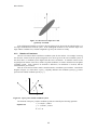
NOTE: distance and total angle change (for variance) are approximations.
3.5
Picking from a Distribution
In the sampling method, we are often confronted with the problem of picking from a particular
distribution. Here we discuss a method for picking from a distribution, based on its cumulative
distribution. Any time we can form the cumulative distribution, this method is applicable.
For a random variable X with density function f X (x ) , the cumulative distribution is defined as
P( X ≤ y ) , that is, the probability that the random variable is less than a value x. From the definition of
probability density, we can write:
y
P( X ≤ y ) =
∫f
X
( x)dx
(3-8)
−∞
We can use the cumulative distribution to define a picking strategy, based on uniform sampling.
Suppose we pick some large number N of samples from X. First note that for any probability a, aN of the
samples should have values taken from the beginning of the distribution f X (x ) up to the point where it
integrates to the probability a. In terms of the cumulative distribution, aN of the samples should be less
than or equal to x a , where
P (X ≤ x a ) = a
(3-9)
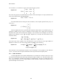
How can we pick the set N? Suppose we start by picking from a uniform distribution in the interval
[0,1]. Let the value picked be called a. Then, we find the x a that satisfies Equation 3-2, and use this
value as a member of N. If we pick the entire set N in this way, it will satisfy Equation 3-2, in the limit of
large N.
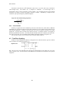
For a standard normal distribution ( N 0,1 ), the cumulative distribution can be found using the error
function. For any value x, the cumulative distribution is:
PN 0 ,1 ( x) =
2) +1
erf ( x
2
(3-10)
To find the value x a that satisfies a = PN 0 ,1 ( x a ) , we have to compute the inverse of the cumulative
distribution. There are several ways to do this, the most common being some variant of Gauss-Newton
iteration. For our purposes, a simple table-driven strategy will be good, because it can also be used for
picking from discrete sample distributions.
In the table method, we pre-compute a table of value of the cumulative function P. Generally, we
will pick entries in the table based on where there are high values of the PDF underlying the cumulative
distribution. For the standard normal function, values from –5 to 5 should suffice, since that is where most
of the probability mass is distributed.. The table can be as fine-grained as required; a reasonable size is
100 entries.
Given a value for a, which is between 0 and 1, the table is searched using recursive binary search.
The middle entry is compared with a, and if it is higher, the search proceeds with the lower half of the
table. If it is lower, the search continues with the upper half. Eventually two successive entries that
21