Download INFORMATIK

INFORMATIK
BERICHTE
352 – 7/2009
Efficient k-Nearest Neighbor Search on
Moving Object Trajectories
Ralf Hartmut Güting, Thomas Behr, Jianqiu Xu
Fakultät für Mathematik und Informatik
Postfach 940
D-58084 Hagen
Efficient k-Nearest Neighbor Search on
Moving Object Trajectories
Ralf Hartmut Güting, Thomas Behr, Jianqiu Xu
Database Systems for New Applications,Mathematics and Computer Science
University of Hagen, Germany
{rhg,thomas.behr,jianqiu.xu}@fernuni-hagen.de
July 25, 2009
Abstract
With the growing number of mobile applications, data analysis on large sets of historical moving objects trajectories becomes increasingly important. Nearest neighbor search is a fundamental
problem in spatial and spatio-temporal databases. In this paper we consider the following problem:
Given a set of moving object trajectories D and a query trajectory mq, find the k nearest neighbors
to mq within D for any instant of time within the life time of mq. We assume D is indexed in a
3D-R-tree and employ a filter-and-refine strategy. The filter step traverses the index and creates a
stream of so-called units (linear pieces of a trajectory) as a superset of the units required to build
the result of the query. The refinement step processes an ordered stream of units and determines the
pieces of units forming the precise result.
To support the filter step, for each node p of the index, in preprocessing a time dependent coverage
function Cp (t) is computed which is the number of trajectories represented in p present at time t.
Within the filter step, sophisticated data structures are used to keep track of the aggregated coverages
of the nodes seen so far in the index traversal to enable pruning. Moreover, the R-tree index is
built in a special way to obtain coverage functions that are effective for pruning. As a result, one
obtains a highly efficient k-NN algorithm for moving data and query points that outperforms the two
competing algorithms by a wide margin.
Implementations of the new algorithms and of the competing techniques are made available as
well. Algorithms can be used in a system context including, for example, visualization and animation
of results. Experiments of the paper can be easily checked or repeated, and new experiments be
performed.
1 Introduction
Moving objects databases have been the subject of intensive research for more than a decade. They allow
one to model in a database the movements of entities and to ask queries about such movements. For some
applications only the time-dependent location is of interest; in other cases also the time dependent extent
is relevant. Corresponding abstractions are a moving point or a moving region, respectively. Examples
of moving points are cars, air planes, ships, mobile phone users, or animals; examples of moving regions
are forest fires, the spread of epidemic diseases and so forth.
Some of the interest in this field is due to the wide-spread use of cheap devices that capture positions,
e.g. by GPS, mobile phone tracking, or RFID technology. Nowadays not only car navigation systems,
but also many mobile phones are equipped with GPS receivers, for example. Vast amounts of trajectory
data, i.e., the result of tracking moving points, are accumulated daily and stored in database systems
[13, 34, 28].
There are two kinds of such databases. The first kind, sometimes called a tracking database, represents a set of currently moving objects. One is interested in continuously maintaining the current
1
positions and to be able to ask queries about the positions as well as the expected positions in the near
future. This approach was pioneered by the Wolfson group [36, 40]. With this approach, a cab company
can find the nearest taxi to a passenger requesting transportation.
The other kind of moving objects database represents entire histories of movement [24, 16], e.g.
the entire set of trips of the vehicles of a logistics company in the last day or even month or year. For
moving points such historical databases are also called trajectory databases. The main interest is in
performing complex queries and analyses of such past movements. For the logistics company this might
result in improvements for the future scheduling of deliveries. For zoologists, the collected movement
information of animals (equipped with a radio transmitter) can be used to analyse their behavior.
There has been a lot of interest in research to support such analyses, for example in data mining
on large sets of trajectories [22], on discovering movement patterns such as flocks or convoys traveling
together [23, 28], on finding similar trajectories to a given one [19], to name but a few. Of course,
indexing and query processing techniques (see [29]) play a fundamental role in supporting such analyses.
In this paper we consider the problem of computing continuous nearest neighbor relationships on a
historical trajectory database. Nearest neighbor queries are, besides range queries, the most fundamental
query type in spatial databases. With the advent of moving objects databases, also time dependent
versions have been studied. One can distinguish four types of queries:
• static query vs. static data objects (i.e., the classical nearest neighbor query)
• moving query vs. static data objects (e.g. maintain the five closest hotels for a traveller)
• static query vs. moving data objects (e.g. observe the closest ambulances to the site of an accident)
• moving query vs. moving data objects (e.g. which vehicles accompanied president Obama on his
trip through Berlin)
Furthermore, one can consider these query types in a tracking database which leads to the notion
of a continuous query, maintaining the result online while entities are moving. This is most interesting
for consumer applications. But one can also consider these queries in the context of analysing historical
trajectories which is the case studied in this paper.
Note that the last of the four query types is the most difficult and general one. It includes all other
cases, as a static object can be represented as a moving object that stays in one place. We will handle this
case.
The precise problem considered is the following. We call the data type representing a complete
trajectory moving point or mpoint, for short [24, 16]. Let d(p, q) denote the Euclidean distance between
points p and q. Let mp(i) denote the position of moving point mp at instant i.
Definition 1 [TCkNN-query] A trajectory-based continuous k-nearest neighbor query is defined as follows: Given a query mpoint mq and a relation D with an attribute mloc of type mpoint, return a subset
D 0 of D where each tuple has an additional attribute mloc0 such that the three conditions hold:
1. For each tuple t ∈ D0 , there exists an instant of time i such that d(t.mloc(i), mq(i)) is among the
k smallest distances from the set {d(u.mloc(i), mq(i))|u ∈ D}.
2. mloc0 is defined only at the times condition (1) holds.
3. mloc0 (i) = mloc(i) whenever it is defined.
In other words, the query selects a subset of tuples whose moving point belongs at some time to the k
closest to the query point and it extends these by a restriction of the moving point to the times when it
was one of the k closest.
2
This query type has been considered in the literature [18, 21] with a further parameter, a query time
interval. However, our definition covers this case as well, since one can easily compute the restriction of
the query trajectory to this time interval first.
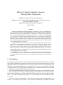
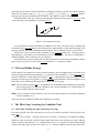
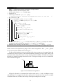
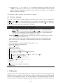
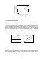
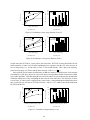
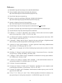
An example of a TCkNN query is shown in Figure 1. To enable easy interpretation of the figure, we
assume that all objects only change their x-coordinate and the y-coordinate is fixed to y0 .
Figure 1: Example of a TCkNN query
Besides the query object mq, there are five moving data objects {o1 , . . . , o5 }. We set k = 2, that
means, we search for the two nearest neighbors. As shown in the figure, the result changes with time.
For example, between t0 and t1 , the result is the set {o1 , o2 } and between t1 and t2 , the result changes to
{o2 , o3 }.
TCkNN queries on the one hand are natural from a systematic point of view as they are the dynamic
version of a fundamental problem in spatial databases. They also have many applications, especially
in discovering groups of entities traveling together with a query object. Some examples are mentioned
in [18, 20]. Further, an efficient solution to this problem might be used as a stepping stone for solving
data mining problems such as discovering flock or convoy patterns. Traffic jams are another example of
groups of vehicles staying close to each other for extended periods of time.
So far, there exist two approaches for handling TCkNN queries [18, 20]. Both use R-tree like structures for indexing the data trajectories, i.e. in [18] a 3D-R-tree is used and in [20] a TB-tree [32] is
utilized. They are discussed in more detail in Section 2.
Our contributions are the following:
• We offer the first filter-and-refine solution, in the form of two different algorithms and query processing operators, called knearestfilter and knearest . The first traverses an index to produce an
ordered stream of candidate units (pieces of movement), the second consumes such an ordered
stream. Both together offer a complete solution. However, knearest can also be used independently. This is important for queries that restrict candidate nearest neighbors by other conditions
so that the index cannot be used.
• We offer a solution that employs novel and highly sophisticated pruning strategies in the filter
step. A fundamental idea is to preprocess coverage functions for each node of the index that
describe how many moving objects are present in the nodes subtree for any instant of time. This is
supported by special techniques to build an R-tree and by efficient data structures and algorithms
to keep track of pruning conditions.
• We provide a thorough experimental comparison which demonstrates that our algorithm is orders
of magnitude faster than the two competing algorithms for larger databases and larger values of k.
• For the first time, such algorithms are made publicly available in a system context and so can be
used for real applications. The S ECONDO system is freely available for download. A new plugin
3
technology exists that makes it easy for readers of this paper to add a nearest neighbor module
(plugin) to an existing S ECONDO installation. All algorithms can then be used in the form of
query processing operators; they can be applied to any data sets that are available in the system or
that users provide; the results can easily be visualized and animated.
• We also provide scripts for test data generation and for the execution of experiments. In this way
easy experimental repeatability is provided. Besides repeating the experiments shown in the paper,
readers can change parameters, explore other data sets, build indexes in other ways, and hence
study the behaviour of these algorithms in any way desired, with relatively little effort. Indeed,
we would like to promote such a methodology for experimental research and view this paper and
implementation as a demonstration of it.
The remainder of this paper is structured as follows. Section 2 surveys related work, especially the
two algorithms solving the same problem as this paper. In Section 3 we briefly describe the representation
of trajectories. Section 4 outlines the filter-and-refine strategy. After that, the filter step is described in
detail in Section 5. First, we give an overview of the basic idea and expose arising subproblems. The
next subsections show how these problems can be solved. Then, the refine step is presented in Section
6. The results of an experimental evaluation comparing our approach with both existing approaches are
shown in Section 7. Section 8 explains how the algorithms can be used in the context of the S ECONDO
system and how experiments can be repeated. Finally, Section 9 concludes the paper and gives directions
for future work.
2 Related Work
There are several types of kNN queries. The most simple case is that both the query point and the data
points are static. The first algorithm for efficient nearest neighbor search on an R-tree was proposed
by [35] using depth-first traversal and a branch-and-bound technique. An incremental algorithm was
developed in [25]. Again, an R-tree is traversed. Here a priority queue of visited nodes ordered by
distance to the query point is maintained. The incremental technique is essential if the number of objects
needed is not known in advance, e.g. if candidates are to be filtered by further conditions. Because in
this case all involved objects are static, also the result is a fixed set of objects.
The first algorithm for CNN (Continuous Nearest Neighbor) queries was proposed in [37]. It handles
the case that only the query object is moving, while the data objects remain static. Here the basic
idea is to issue a query at each sampled or observed position of a query point, trying to exploit some
coherency between the location of the previous and the current query. This algorithm suffers from the
usual problems of sampling. If there are too few sample points, the result may be inaccurate. On the
other hand, many sampling points lead to an increase in computation time without any guarantee for a
correct result.
An improved algorithm was proposed by [39]. Here an algorithm searches the R-tree only once to
find the k nearest neighbors for all positions along a line segment, without the need of sampling points.
There exists a lot of work related to Continuous k Nearest Neighbor queries [38, 27, 33, 31, 42, 41, 9,
26]. In all these approaches tracking databases are assumed and the task is online maintenance of nearest
neighbors for a moving query point, in some cases also for moving data points. For each of these objects
only the current and near future position is known. Index structures like the TPR-tree are used [33, 9]
which indexes current and near future positions; in some cases simple grid structures are employed to
support high update rates [41, 42]. In [9] also reverse nearest neighbor queries are addressed. Iwerks et
al. [27] also support updates of motion vectors.
Note that all this work is fundamentally different from the problem addressed in this paper because
only the current motion vector is known. In contrast, we are considering historical trajectory databases.
In this case, the data set is not only a vector for each moving object, but a complete trajectory, and there
4
is no need to process pieces of a trajectory in a particular order (e.g. in temporal update order). Instead,
the set of trajectories can be organized and traversed in any way that is suitable.
A few works have considered the case of historical trajectory databases and we consider these next
in some detail.
In [21], Gao et al. propose two algorithms for a query point and for a query trajectory, respectively,
on a set of stored trajectories. In contrast to our algorithm, the result is static, i.e. they return the ids
of the k trajectories which ever come closest to the query object during the whole query time interval.
In contrast, our approach will report the k nearest neighbors at any instant for the lifetime of the query
object.
In [18] several types of NN-queries on historical data are addressed. The types depend on whether
the query object is moving or not and whether the query itself is continuous or not. One of the types
corresponds to the TCkNN query defined in Section 1. The authors represent trajectories as a set of
line segments in 3D space (2D + time). The segments are indexed by an R-tree like structure (e.g. 3D
R-Tree, TB-tree or STR-tree). The algorithm is formulated for the special case k = 1 and then extended
to arbitrary values of k. The nodes of the tree are traversed in depth first manner. If a leaf is reached,
the contained line segments are inserted into a structure named nearest containing the distance curves
between the already inserted segments and the segments coming from the query point. Entries whose
minimal distance to the query object is greater than the maximal distance stored in nearest are ignored.
Other segments are inserted extending existing entries if applicable. For a non-leaf node, all children
are checked whether they can be pruned (minimal distance is larger than the maximal distance stored
in nearest during the time interval covered by the node). For an arbitrary k, a buffer of k nearest
structures is used.
In this paper we traverse the tree in breadth first manner. Besides the tree, we determine in preprocessing and store the time dependent number of data objects present in a node’s subtree1 . This allows
pruning nodes using only information of nodes at the same level of the tree reducing the number of nodes
to be considered.
[20] extends the approach of [21] to continuous queries, hence, also to the TCkNN problem. The
entries stored in a TB-tree are inserted into a set of k lists l1 . . . lk . These lists contain distance functions
with links to the corresponding units. For each instant the distance value in list li is smaller or equal
to the distance value in list li+1 . Thus, for each instant the list li contains the distance to the current
i-th neighbor or ∞ if no distance is stored for this instant. The maximum distance stored in a list li is
called P runedist(i). Thereby all objects whose minimum distance is greater than P runedist(k) can be
pruned. The main algorithm traverses a TB-tree in best first manner. A priority queue sorted by minimum
distance contains non-processed nodes of the tree. The queue is initialized with the root of the tree. If
the top element of the queue is a node, it is removed and its entries are inserted into the queue ignoring
those non overlapping the query time interval and those with minDist > P runedist(k). Unit entries
are inserted into the set of lists. The process is finished when the minimum distance of the top entry of
the queue is greater than P runeDist(k) or the queue is exhausted. So, pruning is based on disjoint time
intervals or information from the trajectory entries. A more detailed description is given in Section 7.3.
In contrast, our approach allows pruning using also information of nodes on higher levels of the tree.
Because the refinement step of our algorithm can be used separately, it is possible to combine it with
other filter steps, for example if a query contains additional filter conditions.
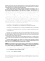
3 Representation of Trajectories
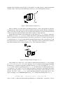
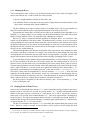
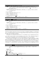
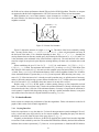
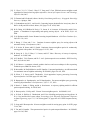
Figure 2 shows the trajectories of two moving points in 3D space. We use the sliced representation [16]
to represent the trajectory of a moving object. A trajectory T =< u1 , u2 , . . . , un > is a sequence of
so-called units. Each unit consists of a time interval and a description of a linear movement during this
1
Actually, we use a simplified version of this moving integer.
5
time interval. The linear movement is defined by storing the positions at the start time and the end time
of the unit. We denote a unit as u = (p1 , p2 , t1 , t2 ), where p1 , p2 ∈ R2 and t1 , t2 ∈ instant. Within a
trajectory, time intervals of distinct units are disjoint. The sequence of units is ordered by time.
In the data model of [24, 16], a trajectory corresponds to a data type moving(point), or mpoint. There
is also a data type corresponding to a unit called upoint.
t
y
x
Figure 2: Two trajectories in space
A set of trajectories can be represented in a database in two ways. The first is to use a relation with
an attribute of type mpoint. Hence each moving object is represented in a single tuple consisting of the
trajectory together with other information about the object. This is called the compact representation.
Second, one can use a relation with an attribute of type upoint. In this case, a moving object is
represented by a set of tuples, each containing one unit of the trajectory. The object is identified by a
common identifier. This is called the unit representation.
In the following we assume that the set D of data trajectories is stored in unit representation, and the
query trajectory is given as a value of the mpoint data type, i.e., a sequence of units.
4 Filter-and-Refine Strategy
We now describe our approach to evaluate a spatio-temporal k-nearest neighbor query. We assume a set
of data moving points in unit representation, i.e., a relation R with an attribute mloc of type upoint. This
relation is indexed by a spatio-temporal (3D) R-tree R mloc containing one entry for each unit. Further
parameters are the query moving point mq of type mpoint, and the number k of nearest neighbors to be
found. We use the well-known filter-and-refine strategy with the two steps:
Filter Traverse the R-tree index R mloc to determine a set of candidate units containing at least all parts
of the moving points of R that may contribute to the k nearest neighbors of mq. Return these as a
stream of units ordered by unit start time.
Refine Process a stream of units ordered by start time to determine the precise set of units forming the
k nearest neighbors of mq.
These two steps are explained in detail in the following two sections.
5 The Filter Step: Searching for Candidate Units
5.1 Basic Idea: Pruning by Nodes with Large Coverage
Obviously the goal of the filter step must be to access as few nodes as possible in the traversal of the
index R mloc.
We proceed as follows. Starting from the root, the index is traversed in a breadth-first manner.
Whenever a node is accessed, each of its entries (node of the next level or unit entry in a leaf) is added to
a queue Q and to a data structure Cover explained below. The Cover structure is used to decide whether
a node or unit entry can be pruned. The entries in Cover and Q are linked so that an entry found to be
6
prunable can be efficiently removed from Q. The question is by what criterion a node can be pruned.
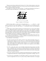
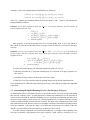
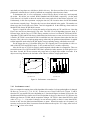
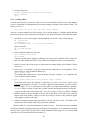
Consider a node N that is accessed and the query trajectory mq. See the illustration in Figure 3.
Figure 3: Nodes and query trajectory mq
Node N contains a set of unit entries representing trajectories. In fact, each segment of a trajectory
is represented as a small 3D box, but we have nevertheless drawn the trajectories directly. Furthermore,
node N looks like a leaf node. However, if it is an inner node of the R-tree, we may still consider the set
of units or trajectories represented in the entire subtree rooted in N in the same way.
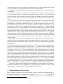
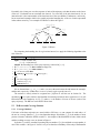
Suppose that at any instant of time within node N s time interval [N .t1 , N.t2 ] at least n trajectories
are present in N and n ≥ k. Let M be a further node and M s time interval be included in N s time
interval. Furthermore let the minimal distance between the xy-projection of M and the xy-projection of
mq (restricted to [M.t1 , M.t2 ]) be larger than the maximal distance between the xy-projection of N and
the xy-projection of mq (restricted to [N.t1, N.t2]). Then node M and its contents can be pruned as
they cannot contribute to the k nearest neighbors of mq. This is illustrated in Figure 4.
Figure 4: Pruning criterion of Lemma 1, k = 5
More formally, for a node K let box (K) denote its spatiotemporal bounding box, i.e., the rectangle
[K.x1 , K.x2 , K.y1 , K.y2 , K.t1 , K.t2 ]. For a trajectory u let box (u) denote its spatiotemporal bounding
box and let u[t1 , t2 ] denote its restriction to the time interval [t1 , t2 ]. For a 3D rectangle B = [x1 , x2 , y1 ,
y2 , t1 , t2 ] let Bxy denote its spatial projection [x1 , x2 , y1 , y2 ] and Bt denote its temporal projection [t1 ,
t2 ], respectively. For a node K, let CK (t) denote the number of trajectories represented in the subtree
rooted at K present at instant t. CK (t) is a function from time into integer values, called the coverage
function. Let C(K) = mint∈[K.t1 ,K.t2] CK (t) be called the (minimal) coverage number of K. For a
(hyper-) rectangle r in a d-dimensional space Rd let points(r) denote all enclosed points of Rd , i.e,
points(r) = {(x1 , . . . , xd ) | r.b1 ≤ x1 ≤ r.t1 , . . . , r.bd ≤ xd ≤ r.td }
where r.bi and r.ti denote the bottom and top coordinates of r in dimension i, respectively. For two
7
rectangles r and s their minimal and maximal distances are defined as
mindist (r, s) = min{d(p, q)|p ∈ points(r), q ∈ points(s)}
maxdist (r, s) = max {d(p, q)|p ∈ points(r), q ∈ points(s)}
where d(p, q) denotes the Euclidean distance between two points p and q. Then we can formulate the
pruning condition as follows.
Lemma 1 Let M and N be nodes of the R-tree R mloc, mq the query trajectory, and k the number of
nearest neighbors desired. Then
C(N ) ≥ k
boxt (M ) ⊆ boxt (N )
mindist (boxxy (M ), boxxy (mq[boxt (M )]) >
maxdist (boxxy (N ), boxxy (mq[boxt (N )])
⇒ M can be pruned.
∧
∧
More generally, several nodes together may serve to prune another node M if for any instant of
time within M s time interval the sum of their coverages exceeds k and they are all closer to the query
trajectory.
Lemma 2 Let S be a set of nodes of the R-tree R mloc, S(t) = {s ∈ S|t ∈ boxt (s)} the nodes of S
present at time t, and M ∈
/ S another node. Let mq be the query trajectory, and k the number of nearest
neighbors desired.
P
∀t ∈ boxt (M ) : s∈S(t) C(s) ≥ k
(∀s ∈ S :mindist(boxxy (M ), boxxy (mq[boxt (M )]) >
∧
maxdist (boxxy (s), boxxy (mq[boxt (s)]))
⇒ M can be pruned.
To realize this pruning strategy, the following subproblems need to be solved:
• Efficiently determine the xy-projection bounding box of a restriction of the query trajectory to a
time interval.
• Determine coverage numbers for the nodes of the R-tree index.
• Define the Cover data structure needed for pruning and provide an efficient implementation.
These subproblems are addressed in the following subsections. After that, the complete filter algorithm
is described.
5.2 Determining the Spatial Bounding Box for a Partial Query Trajectory
As mentioned in Section 3, the query trajectory is represented basically as an array of units with distinct
time intervals, ordered by time. A simple approach to compute the bounding box for the restriction to
some time interval (called the restriction bounding box) is to search the unit containing the start time of
the interval using a binary search. For the (sub-) unit the bounding box is computed. Then the sequence
of units is scanned until the end of the interval is reached. The union of the bounding boxes of all visited
units yields the final result. Here the union of two rectangles is defined as the smallest enclosing rectangle
of the two arguments. If the interval is long, a lot of units must be processed. For example, if the time
interval covers the lifetime of the query trajectory, all units have to be visited.
To enable efficient computation of a restriction bounding box we compute at the beginning of the
filter step an alternative representation of the query trajectory, called a BB-tree (bounding box tree).
8
Essentially it is a binary tree over the sequence of units of the trajectory such that the units are the leaves
of the tree. Each node has an associated time interval. For a leaf this is the unit time interval, for an
internal node it is the concatenation of the time intervals of the two children. Furthermore, each node p
has an associated rectangle which is the spatial projection bounding box of the set of units represented
in the subtree rooted in p. An example of a BB-tree is shown in Figure 5.
([t0 , t6 ],
S6
i=1 ri )
([t0 , t4 ], r1 ∪ r2 ∪ r3 ∪ r4 )
([t0 , t2 ], r1 ∪ r2 )
([t4 , t6 ], r5 ∪ r6 )
([t2 , t4 ], r3 ∪ r4 ) ([t4 , t5 ], r5 ) ([t5 , t6 ], r6 )
([t0 , t1 ], r1 ) ([t1 , t2 ], r2 ) ([t2 , t3 ], r3 ) ([t3 , t4 ], r4 )
Figure 5: BB-tree
For computing the bounding box for a given time interval, we apply the following algorithm to the
root of the tree:
Algorithm 1: get box(n, t1 , t2 )
Input: n - node of a bbox-tree;
[t1 , t2 ] - a time interval.
Output: the bounding box of the query trajectory, restricted to [t1 , t2 ]
1 if t1 > n.t2 ∨ t2 < n.t1 then return an empty box;
2 if t1 ≤ n.t1 ∧ t2 ≥ n.t2 then return n.r ;
3 if n is an inner node then
4
return get box(n.left) ∪ get box(n.right) ;
5
6
7
8
else
let u be a copy of n.u;
restrict u to [t1 , t2 ];
return bbox(u);
We use the notations n.t1 , n.t2 , n.r, and n.u to access the start instant, the end instant, the rectangle,
and the unit, repectively. Furthermore, we use n.left and n.right to get the sons of n.
The structure is closely related to a segment tree [14] that we will also use in Section 5.4. The
algorithm get box is quite similar to the algorithm for inserting an interval into a segment tree. It is well
known that the time complexity is O(log n) where n is the number of leaves of the tree (units of the
query trajectory). The BB-tree can be built in linear time.
5.3 3D R-tree and Coverage Number
5.3.1
Coverage Numbers
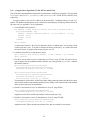
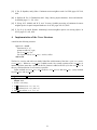
If all units of the data trajectories are stored within a 3D R-tree, we can compute for each node n of
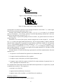
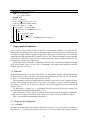
the tree its coverage function Cn (t), a time dependent integer. Recall that Cn (t) is the number of units
present at instant t within the subtree rooted in n. An example of the distribution of units within a node
and the resulting coverage curve are shown in Figure 6.
In Section 5.1 we have seen that for pruning only one number C(n), the minimal coverage number, is
used. This would be 1 in Figure 6. Now it is easy to see that due to boundary effects only a small number
9
N
Unit
u8
u7
u6
u5
u4
u3
u2
u1
6
5
4
3
2
1
t0 t1 t2 t3 t4 t5 t6 t t0 t1 t2 t3 t4 t5 t6 t
(a) units on time
(b) coverage function
Figure 6: Coverage Function
of units will be present at the beginning or end of a node’s time interval. Hence if we use simply the
minimum of the coverage function, no good pruning effect can be achieved. On the other hand, within a
reduced time interval, e.g. from t1 to t5 , a large minimal coverage could be observed.
The idea is therefore to use instead of one coverage number three of them, by splitting a node’s
time interval into three parts, namely two small parts at the beginning and end with small coverage
numbers, and a large part in the middle with a large coverage number. In Figure 6 we could use
([t0 , t1 ], 1), ([t1 , t5 ], 5), ([t5 , t6 ], 2).
We introduce an operator to compute from the coverage function the three numbers, called the hat
operator (because the shape of the curve reminds of a hat). Technically it takes an argument c of type
moving integer or mint, describing the coverage function, and returns an mint r with the following
properties:
• deftime(r) = deftime(c)
• ∀t ∈ deftime(r) : r(t) ≤ c(t)
• r consists of three units at most
• the area under curve r is the maximum of all possible areas fulfilling the first three conditions
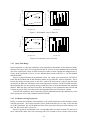
An application of the hat operator is shown in Figure 7.
N
N
6
5
4
3
2
1
6
5
4
3
2
1
t0 t1 t2 t3 t4 t5 t6 t
t0 t1 t2 t3 t4 t5 t6 t
(b) result of hat
(a) coverage curve
Figure 7: Application of the hat operator
Intuitively it is good for pruning if a large coverage number is obtained over a long time interval.
The goal is therefore to maximize the area of the “middle” unit of the result which is the product of these
quantities. Using a stack, the simplification of the curve can be done in linear time with respect to the
10
Algorithm 2: hat(c)
Input: c - an mint (moving integer) describing a coverage function
Output: a reduced mint with only three units
1 let s be a stack of pairs < t, n >, initially empty;
2 let int area = 0;
3 extend c by a pseudo unit <[c.t2 , c.t2 + 1], 0]>;
/* ensures that all entries are popped from stack at the end
4 for each unit u in c do
5
if s is empty then s.push(< u.t1 , u.n >) else
6
if s.top().n < u.n then s.push(< u.t1 , u.n >) else
7
tend = u.t1 ;
8
while s.top().n > u.n do
9
< tstart , cn >= s.top(); s.pop();
10
if area == 0 then
11
area = (tend − tstart ) × cn;
12
< t1 , t2 , n >=< tstart , tend , cn >;
13
14
15
16
17
18
19
20
*/
else
newarea = (tend − tstart ) × cn;
if newarea > area then
area = newarea;
< t1 , t2 , n >=< tstart , tend , cn >;
s.push(< tstart , u.n >)
Now the middle unit is < t1 , t2 , n >. Scan the units before t1 and after t2 to compute the minimal
coverages first and last for the time intervals [c.t1 , t1 ] and [t2 , c.t2 ], respectively;
return the mint consisting of the three units ([c.t1 , t1 ], f irst), ([t1 , t2 ], n), and ([t2 , c.t2 ], last);
number of units of the original moving integer. This is shown in Algorithm 2. Here c.t1 and c.t2 denote
the start and end of the definition time of moving int c.
The idea of this algorithm is to process the units of the given coverage curve in temporal order and
to maintain on a stack a sequence of units with monotonically increasing coverage values. When a unit
is encountered that reduces the current coverage, then the potential candidates for middle units ending at
this point are examined by taking them from the stack. The largest rectangle seen so far is maintained.
This is illustrated in Figure 8.
Cov.
a
b
c
u
t
Figure 8: Stack maintained in Algorithm 2
In Figure 8, when unit u is encountered, the last three stack entries a, b, and c with higher coverage
values than that of u are popped from the stack, and for each of them the size of the respective rectangle
is computed. Start time, end time, and coverage of the largest rectangle so far are kept.
11
5.3.2
Building the R-tree
This section describes how an R-tree over the data point units can be built, which will support k-NN
queries in an efficient way. A node of the R-tree can be pruned if
• there are enough candidates available in other nodes, and
• the minimum distance of the node to the query point is higher than the maximum distance of the
query point to each node in the current candidate set.
The first condition can be achieved with a small set of candidate nodes if the coverage numbers are
high. The second condition requires a good spatial distribution of the nodes of the R-tree.
Experiments have shown that if we fill the R-tree either by the standard insertion algorithm or by a
bulkload [11, 12] using z-order [30], for example, only the spatial distribution of the nodes will be good.
But the coverage numbers will be very small and a large candidate set is required.
However, by using a customized bulkload algorithm for filling the R-tree, we can achieve some
control over the distribution of the R-tree nodes. The bulkload works as follows: It receives a stream of
entries (bounding box and a tuple id) and puts them into a leaf of the R-tree until either the leaf is full or
the distance between the new box and the current bounding box of the leaf exceeds a threshold. When
this happens, the leaf is inserted into a current node at the next higher level and a new leaf is started. In
this way, the tree is built bottom-up.
This bulkload algorithm itself does not care about the order of the stream. So by changing the order,
the structure of the R-tree is affected. For example, if we sort the units by their starting time, temporally
overlapping units are inserted into the same node and the coverage number is very high. But this order
ignores spatial properties and so the nodes will have many and large overlappings in the xy-space.
To get both, high coverage numbers and good spatial distribution, we do the following. We partition
the 3D space occupied by the units into cells, using a regular grid. The spatial partition (or cell size) is
chosen in such a way that within a cell, at each instant of time, on the average about p units are present.
Then the temporal partition is chosen such that within a cell enough units are present to fill on the average
about r nodes of the R-tree. A stream of units to be indexed is extended by three integer indices x, y, t
representing a spatiotemporal cell containing the unit2 , hence has the form < unit, tupleid, x, y, t >.
The stream is then sorted lexicographically by the four attributes < t, x, y, unit > where the order
implied by the fourth attribute is unit start time. In this way, a subsequence of units belonging into one
cell is formed and these are ordered by start time. Such subsequences are packed by the bulkload into
about r nodes of the R-tree, resulting in nice hat shapes as desired in Section 5.3.1.
We do not yet have a deep theory for the choice of numbers p and r. In our experiments, p = 15 and
r = 6 have worked quite well.
5.4 Keeping Track of Node Covers
In this section we describe the data structure Cover used to control the pruning of nodes or unit entries.
Suppose a node N of the R-tree is accessed, its coverage number3 is n = 8, and its minimal and maximal
distance to the query trajectory, restricted by N 0 s time interval, are d1 and d2 , respectively. Assume a
further node M is accessed whose minimal distance is d3 . This can be represented in a 2D diagram as
shown in Figure 9. The edge for the minimal distance of node N is called the lower bound, denoted N −
and drawn thin, the edge for the maximal distance is called the upper bound, denoted N + and drawn fat.
As discussed before, if k ≤ 8, M can be pruned.
The idea is to maintain a data structure Cover representing this diagram during the traversal of the
R-tree. Whenever a node is accessed, its lower bound is used as a query to check whether this node
2
containing one of its corner points, for example
In this section, for simplicity we assume a node has a single coverage number instead of the three coverages computed by
the hat operator. The modification to deal with three numbers is straightforward.
3
12
Figure 9: Representing node coverages, one node
Figure 10: Representing node coverages, many nodes
can be pruned. If it cannot be pruned, its lower and upper bounds are entered into Cover, and its upper
bound is also used to prune other entries from Cover.
An upper or lower bound is represented as a tuple b = ([t1 , t2 ], d, c, lower) where [t1 , t2 ] is the time
interval, d the distance, c the coverage, and lower a boolean flag indicating whether this is the lower
bound. We also denote the coverage as C(b) = b.c.
Whereas Figure 9 represents the pruning criterion of Lemma 1, the general situation of Lemma 2 is
shown in Figure 10.
When node M is accessed, first a query with the rectangle below its lower bound M − is executed
on Cover to retrieve the upper bounds intersected by it. The set of upper bounds U found is scanned in
temporal order, keeping track of aggregated coverage numbers, to determine whether M can be pruned.
Let Cmin be the minimal aggregate coverage of bounds in U . If k ≤ Cmin , M can be pruned. If M
cannot be pruned, it is inserted into Cover. If k ≤ C(M ) + Cmin , a second query with the rectangle
above the upper bound M + is executed, retrieving the lower bounds contained in it. All nodes to which
these lower bounds belong, are pruned.
From this analysis, we extract the following requirements for an efficient implementation of the data
structure Cover:
1. It represents a set of horizontal line segments in two-dimensional space.
2. It supports insertions and deletions of line segments.
3. It supports a query with a point p to find all segments below p.
4. It supports a query with a line segment l to find all left or right end points of segments below l or
above l (pruning lower bounds above M+).
Two available main memory data structures that fulfill related requirements are a segment tree [14] and
a standard binary search tree. The segment tree
• represents a set of intervals
• supports insertion and deletion of an interval
• supports a query with a coordinate 4 p to find all intervals containing p.
The binary search tree
4
We call a single value from a one-dimensional domain a coordinate.
13
f
f
a
c
C
A
C
b
a
B b
B
C c
p
A
B
C
Figure 11: The Cover structure, a modified segment tree
• represents a set of coordinates (start and end instants of time intervals, in this case).
• supports insertion and deletion of coordinates.
• supports range queries, i.e., queries with an interval to find all enclosed coordinates.
We might use these two data structures separately to implement Cover, but instead we employ a slightly
modified version of the segment tree that merges both structures into one. Such a structure is shown in
Figure 11.
The segment tree is a hierarchical partitioning of the one-dimensional space. Each node has an
associated node interval (drawn in Figure 11); for an internal node this is equal to the concatenation of
the node intervals of its two children. A segment tree represents a set of (data) intervals. An interval
is stored in a segment tree by marking all nodes whose node intervals it covers completely, in such a
way that only the highest level nodes are marked (i.e., if both children of a node could be marked then
instead the father is marked). Marking is done by entering an identifier of (pointer to) the interval into
a node list. For example, in Figure 11 interval B is stored by marking two nodes. It is well-known that
an interval can only create up to two entries per level of the tree, hence a balanced tree with N leaves
storing n intervals requires O(N + n log N) space. A coordinate query to find the enclosing intervals
follows a path from the root to the leaf containing the coordinate and reports the intervals in the node
lists encountered. This takes O(log N + t) time where t is the number of answers. For example, in Figure
11 a query with coordinate p follows the path to p and reports A and B.
The segment tree is usually described as a semi-dynamic structure where the hierarchical partitioning
is created in advance and then intervals are inserted or deleted just by changing node lists. We use it here
as a fully dynamic structure by first modifying the structure to accomodate new end points and then
marking nodes. When new end points are added, they are also stored in further node lists node.startlist
and node.endlist (besides the standard list for marking, node.list). In Figure 11 entries for end points are
shown as lower case letters. The thin lines in Figure 11 show the structure after insertion of intervals A
and B. The fat lines show the modification due to the subsequent insertion of interval C. The structure
now also supports range queries for end points, like a binary search tree. If the tree is balanced, the time
required for a range query is O(log N + t) for t answers.
In our implementation we use an unbalanced tree which is very easy to implement. The unbalanced
structure does not offer worst case guarantees but behaves quite well in practice, as will be shown in the
experiments.
The interface to the Cover structure is provided by the four methods:
• insert entry(ce). ce is a cover entry, defined below. Inserts it by its time interval.
• delete entry(ce). Deletes entry ce from the node lists (but does not shrink the structure).
• point query(n, t), n a node, t an instant of time. Returns all entries whose time interval contains t.
14
• range query(n, t1 , t2 ). n is a node, [t1 , t2 ] - a time interval. Returns a list of pairs of the form
<which, ce> where which ∈ {bottom, top}, ce a cover entry (bottom indicates a start time, top an
end time). The list contains only entries whose start or end time lies within [t1 , t2 ], in temporal
order w.r.t their start or end time.
The algorithms for these operations can be found in the Appendix.
5.5 The Filter Algorithm
We are now able to describe the filter algorithm, called knearestfilter, precisely. It uses subalgorithms
node entry and unit entry to create entries for the Cover structure. It further employs a method insert and prune of the Cover structure with its subalgorithms mincover and prune above. These algorithms are shown on the next pages (Algorithms 3 through 8).
Algorithm 3: knearestfilter(R, R mloc, Cov, Cov nid, mq, k)
Input: R - a relation with moving points in unit representation, i.e., with an attribute mloc of type
upoint ; R mloc - a 3D R-tree index on attribute mloc of R; Cov - a relation containing
coverage numbers for each node of the R-tree R mloc; Cov nid - a B-tree index on the nid
attribute of Cov representing the node identifier of the R-tree; mq - a query trajectory of
type mpoint; k - the number of nearest neighbors to be found.
Output: an ordered set of candidate units, ordered by unit start time, containing all parts of the k
moving points of R closest to mq;
1 let Q be a queue of nodes of the R-tree, initially empty; (To be precise, Q contains pairs of the
form <node, coverptr> where node is a node of the R-tree and coverptr is a pointer into the
Cover data structure.
2 let Cover be the Cover structure, initialized with node(-∞,+∞);
3 let mqbb be a BB-tree representing mq;
4 node r = R mloc.root();
5 Q.enqueue(<r, null>);
6 while Q is not empty do
7
<r, coverptr> = Q.dequeue();
8
if coverptr 6= null then Cover.delete entry(coverptr);
9
for each entry c of r do
10
if r is an inner node then ce=node entry(c, mqbb, Cov, Cov nid);
11
else ce = unit entry(u, mqbb);
Cover.insert and prune(ce, k, Q, c);
12
16
S = Cover.range query(Cover.root(), -∞,+∞);
Cand = ∅;
for each < which, s >∈ S do
if which = bottom then Cand.append(s);
17
return Cand;
13
14
15
6 Refinement
The problem to be solved in the refinement step is to compute for a sequence of units, arriving temporally
ordered by start time, a sequence of units (that may be equal to an input unit or a part of it) that together
form the k nearest neighbors over time. For each arriving unit, its time dependent distance function to
the query trajectory is computed. Depending on whether the unit overlaps one or more units of the query
15
Algorithm 4: node entry(n, mqbb, Cov, Cov nid)
Input: n - a node of the R-tree; mqbb - the query trajectory represented as a BB-tree; Cov - a
relation containing coverage numbers for nodes of the R-tree; Cov nid - a B-tree index on
node identifiers of Cov.
Output: an entry for the Cover data structure, of the form <[t1 , t2 ], mindist, maxdist, cn,nodeid,
tid, queueptr, refs>.
1 [t1 , t2 ] = boxt (n);
2 let box = mqbb.getBox(mqbb.root(), t1 , t2 );
3 mindist = mindist(boxxy (n), box);
4 maxdist = maxdist(boxxy (n), box);
5 cn = getcover(n.id, Cov, Cov nid);
6 return new entry <[t1 , t2 ], mindist, maxdist, cn, n.id, ⊥, null, ∅ >;
Algorithm 5: unit entry(n, mqbb)
Input: u - a unit entry from a leaf of the R-tree; mqbb - the query trajectory represented as a
BB-tree.
Output: an entry for the Cover data structure, of the form <[t1 , t2 ], mindist, maxdist, cn,nodeid,
tid, queueptr, refs>.
1 [t1 , t2 ] = boxt (n);
2 let box = mqbb.getBox(mqbb.root(), t1 , t2 );
3 mindist = mindist(boxxy (n), box);
4 maxdist = maxdist(boxxy (n), box);
5 return new entry <[t1 , t2 ], mindist, maxdist, 1,⊥, u.tid, null, ∅ >;
trajectory, the distance function may consist of several pieces with different definition. It is well-known
(see e.g. [16]) that the distance between two moving point units with the same time interval is in general
the square root of a quadratic polynomial.
The problem is to compute the intersections of a set of distance curves to determine the lowest k
curves, and to return the parts of units corresponding to these pieces. This is illustrated in Figure 12
where the units corresponding to the two lowest of three distance curves are to be returned.
The intersections of the distance curves can be found efficiently by slightly modifying the standard
plane sweep algorithm for finding intersections of line segments by Bentley and Ottmann [10]. The
basic idea of that algorithm is to maintain the sequence of line segments (curves in our case) intersecting the sweep line. Encountering the left end of a curve (within the sweep event structure ordered by
t-coordinates), it is inserted into the sweep status structure, checking the two neighboring curves for
Algorithm 6: insert and prune(ce, k, Q, c)
Input: ce - a cover entry of the form <[t1 , t2 ], mindist, maxdist, cn, nodeid, tid, queueptr,refs>; k
- the number of nearest neighbors to be found; Q - a queue of nodes; c - a node or unit
entry.
Output: none
1 int mc = mincover(ce);
2 if mc < k then
3
insert entry(ce);
4
if c is a node then ce.queueptr = Q.enqueue(<c, ce>);
5
if mc + ce.cn ≥ k then prune above(ce, Q);
16
Algorithm 7: mincover(ce)
Input: ce - a cover entry
Output: Cmin , the minimal aggregate coverage below the lower bound of ce.
1 let root = this.root();
2 let S1 = point query(root, ce.t1 );
3 int c = 0;
4 for each s ∈ S1 do
5
if s.maxdist < ce.mindist then c = c + s.cn;
13
Cmin = c;
let S2 = range query(root, ce.t1 , ce.t2 );
for each <which, s> ∈ S2 do
if s.maxdist < ce.mindist then
if which = bottom then c = c + s.cn;
else
c = c - s.cn ;
if c < Cmin then Cmin = c;
14
return Cmin ;
6
7
8
9
10
11
12
d
sweep line
t
Figure 12: Computing the lowest k distance curves
possible intersections. Any intersections found are entered into the event queue of the sweep for further
processing. Encountering the right end of a curve, it is removed from the sweep status structure, checking
the two curves above and below for intersection. Encountering an intersection found previously, the two
intersecting curves are swapped, and the two new pairs of curves becoming neighbors are checked for
intersections. For the sweep status structure, a balanced tree can be used. Whereas computing the intersections of two quadratic polynomials (which can be used directly instead of the square roots) is slightly
more difficult than finding the intersection of two line segments, the basic strategy of the algorithm [10]
works equally well here.
Because units arrive in temporal order, one can scan in parallel the sequence of incoming units, the
priority queue of upcoming events, and the query trajectory mq. The time interval of an incoming unit u
is either enclosed in the time interval of the current unit mu of mq or extends beyond it. If it is enclosed,
an event for deleting this distance curve from the sweep status structure at the end time u.t2 is created. If
the time interval extends beyond that of mu, the distance curve is computed until mu.t2 and two events
for deleting the curve at time mu.t2 and for handling the remaining part of u are created.
Since the focus of this paper is on the filter step, and the refinement step is relatively straightforward,
we omit further details here.
17
Algorithm 8: prune above(ce, Q)
Input: ce - a cover entry;
Q - a queue of nodes.
Output: none
1 let root = this.root();
2 let S = range query(root, ce.t1 , ce.t2 );
3 let ht be a hashtable, initially empty;
4 for each <which, s> ∈ S do
5
if s.mindist > ce.maxdist then
6
if which = bottom then ht.insert(s);
7
else
8
if ht.lookup(s) then
9
delete entry(s);
10
if s.queueptr 6= null then Q.dequeue(s.queueptr);
7 Experimental Evaluation
In this section, we first describe the data sets used for an experimental evaluation of our approach. We
then consider some properties of the proposed algorithm, namely selection of grid sizes, the time required
to compute coverage numbers in preprocessing, and the effectiveness of the filter step. We explain the
implementation of the algorithms HCNN and HCTkNN [18, 20]. The three algorithms are then compared
varying the size of the data set, the parameter k, and the query time interval. A further evaluation on very
long trajectories completes the experiments.
For the experiments a standard PC (AMD Athlon XP 2800+CPU, 1GB memory, 60GB disk) running
SUSE Linux (kernel version 2.6.18) is used. All algorithms were implemented within the extensible
database system S ECONDO [8].
7.1 Data Sets
In the performance study, we use three different data sets. One of them contains real data obtained from
the R-tree Portal [3]. Here, 276 trucks in the Athens metropolitan area are observed. We call this data
set Trucks. It was also used in earlier experiments in [18, 20].
The second data set simulates underground trains in Berlin. In the basic version it contains 562 trips
of trains. We will enlarge this data set by a scale factor n2 by making n2 copies of each trip, translating
the geometry n times in x and n times in y-direction. We call the original data set Trains and derived
data sets Trains n2 .
The third data set – called Cars – is a simulation of 2,000 cars moving on one day in Berlin. This
was obtained from the BerlinMOD Benchmark [1, 15].
From each data set, 10 query objects are selected. In later experiments, the running time and number
of page accesses of a query is measured as the average over 10 queries using these different objects.
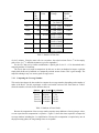
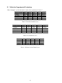
Table 1 lists detailed information about the data sets.
7.2 Properties of Our Approach
7.2.1
Grid Sizes
Grid sizes for our approach are determined as described in Section 5.3.2. For the original Trains data set
this results in a 3 x 3 spatial grid (of which in fact only 3 x 2 cells contain data) and a temporal partition
18
Name
Trucks
Cars
No.
of
Objects
276
No. of
Units
X-Range
Y Range
111,922
2,000
2,274,218
562
51,444
Trains9
5,058
462,996
Trains25
14,050
1,286,100
Trains64
35,968
3,292,416
Trains100
56,200
5,144,400
Trains
[0, 44541.6]
[0, 53956.7]
[-10836, 32842]
[-6686, 28054]
[-3560, 25965]
[1252, 21018]
[26440, 115965]
[31252, 111018]
[26440, 175965]
[31252, 171018]
[26440, 265965]
[31252, 261018]
[26440, 325965]
[31252, 321018]
average
lifetime
of
an
object
10 hours
24 hours
1 hour
1 hour
1 hour
1 hour
1 hour
Table 1: Statistics of Data Sets
of size 5 minutes. Using the same cell size everywhere, the scaled versions Trains n2 in fact employ
grids of size (3n)2 . A detailed calculation is given in Appendix C.
For the Cars data set by similar considerations a spatial grid of size 12 x 12 is determined and a
temporal partition of 30 minutes.
The Trucks data set is small in comparison. In this case we have not bothered to impose a grid but
simply built the R-tree by bulkload on a temporally ordered stream of units. This is good enough. The
temporal ordering in any case creates good coverage curves.
7.2.2
Computing the Coverage Number
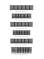
This section investigates the time needed to compute the coverage numbers depending on the number of
nodes of the R-tree. For this experiment, we have used scaled versions of the Trains data set. Table 2
shows the numbers of nodes for the different data sets.
data set
Trains
Trains9
Trains25
Trains64
Trains100
no. of units
51,444
462,996
1,286,100
3,292,416
5,144,400
no. of nodes
847
7,701
21,437
54,986
85,895
Table 2: Numbers of R-tree Nodes
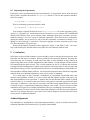
Because the computation of the coverage number requires many additions of moving integer values,
we can expect that this computation is expensive. Figure 13 shows the times required to compute the
coverage numbers including the hat simplification. Because this computation is required only once in
the preprocessing phase, the long running times are acceptable.
19
total running time (sec)
3500
3000
2500
2000
1500
1000
500
0
90
80
70
60
50
40
30
20
10
0
00
00
0
0
0
0
0
0
00
00
0
00
00
0
0
00
00
00
number of nodes in 3D R-tree
Figure 13: Time to Compute the Coverage Numbers
7.2.3
Effectiveness of the Filter Step
number of candidates (x 100)
number of candidates (x 100)
In this section we measure how many candidate units are created by the filter step. This number reflects
the pruning ability of the filtering algorithm which has great influence on the query efficiency because
the units passing the filter step must be processed in the cost intensive refinement step.
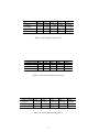
For the first experiment, we have varied the data size. As data sets we have used scaled versions
of Trains. The number of requested nearest neighbors was set to k = 5, the query time to Qt = 1.
The query was performed with a query object available in all data sets, train111. The result is shown in
Figure 14(a). Also the number of units of the final result is part of this figure. One can see that the filter
step returns roughly the same number of candidates for all data sizes.
Second, we have varied the number k of requested neighbors for the data set Trains25. Here a query
object train742 was used in all queries. Figure 14(b) depicts the behaviour of our algorithm. When k
increases, the number of candidates returned by the filter algorithm increases proportional to the final
result.
14
12
10
TCkNN
final result
8
6
4
2
0
0
1
2
3
4
5
120
TCkNN
final result
100
80
60
40
20
0
0
5
10
15
20
25
30
35
40
45
50
k
moving data size (million)
(a) Parameter Datasize
(b) Parameter k (Trains25)
Figure 14: The number of units returned by the filter step
7.3 Competitors’ Implementation
To be able to compare our solution with the two existing algorithms, we have implemented both the
HCNN [18] algorithm and the HCTkNN [20] algorithm within the S ECONDO-framework. Because
HCTkNN uses a TB-tree [32] for indexing the moving data, the TB-tree was also implemented as an
index structure in S ECONDO. HCNN applies the depth first-first method to traverse the index structure
where both a TB-tree and a 3D R-tree can be used. From the experimental results in [18] we know that
20
the 3D R-tree has a better performance than the TB-tree for the HCNN algorithm. Therefore we compare
our approach with this faster implementation. HCTkNN traverses the TB-tree in best first manner.
Both algorithms use a set of data structures, whose elements are so-called nearest lists, to store
the result found so far when traversing the index. The size of this set corresponds to k, the number of
neighbors searched.
D(t)
prunedist (i = k)
split point
D1
D2
list[i]
bc
D3
bc
t
t0
t1
t2
t3
t4
Figure 15: Nearest List Structure
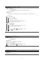
Figure 15 depicts the structure of a single nearest list. The entries of the list are ordered by starting
time. An entry has the form e =< tid, D, t1 , t2 , mind, maxd >, where tid corresponds to an entry in
the leaf node of the index, D is a function depending on time, D(t) = a · t2 + b · t + c, denoting the
moving distance between the entry and the query object during the time interval [t1 , t2 ], mind and maxd
is the maximum or the minimum value of that function, respectively. The time intervals of the entries
stored in a single list are pairwise quasi disjoint, meaning that they can share only a common start or end
point.
When considering the set of k lists list[1], . . . , list [k], for each instant t, list[i].D(t) ≤ list[i +
1].D(t), 1 ≤ i < k, holds. The maximum value stored in list[i] is called prunedist (i). If the union of the
time intervals of the entries in list[i] does not cover the complete query time interval then prunedist (i) =
∞ holds. Thus prunedist (k) is the maximum distance of the k nearest neighbors found so far. All entries
whose minimum distance is greater than prunedist (k) can be pruned. When inserting a new entry e, we
start at list[1]. If the time interval of e is already covered by another entry, we split the entries if necessary
and try to insert the entries having a greater distance function into list[2]. So high values move up within
the set of lists until list[k] is reached or their time interval is not any more covered.
Besides using prunedist, HCNN applies a further pruning strategy to filter impossible non-leaf
nodes. For each entry in non-leaf node, it checks the maximum distance of already stored tuples in the
list restricted to the entry’s life time. If the minimum distance of an entry is larger than the maximum, it
can be pruned. Compared with the pruning strategy with only a global maximum distance, it can prune
more nodes whose time interval is disjoint with that covered by prunedist.
7.4 Evaluation Results
In this section we compare the performance of the three algorithms. Tables with numeric results for all
graphs of this section can be found in Appendix B.
7.4.1
Varying Data Size
In the first experiment, we vary the data size N where all other parameters remain unchanged. We set k
to five, so that each query object asks for its five nearest neighbors. Regarding the query time interval,
the default is to use the entire life time of the query object, i.e., Qt = 1.
Originally we had built the 3D R-tree for HCNN by applying the regular R-tree insertion algorithm
to a stream of units ordered by start time. The authors had informed us that they had used this method to
build the R-tree in their experiments [17]. However, in our experiments we found that HCNN behaves
21
quite badly on large data sets with R-trees built in this way. We discovered that it has a much better
performance when the R-tree is built by bulkload on a temporally ordered stream of units.
To demonstrate this, in a few experiments we have built the R-tree in both ways and compared
the results. We call the two versions HCNN-Standard and HCNN-Bulk, respectively. On the small
Trucks data set it is feasible to show the results in the same graph; this is done below in Section 7.4.3.
Unfortunately, in this first experiment varying the data size, the execution times for HCNN-Standard
soon become extremely large. Therefore they have not been included in the graphs. The numbers are
shown up to the Trains9 data set in Tables 3 and 4 in Appendix B. In the following, when results are
labeled HCNN, always HCNN-Bulk is meant.
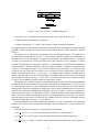
Figure 16 reports the effect of varying the number of moving units on CPU and I/O cost. Note that
Figure 16(a) and (b) are plotted using a log scale. The CPU cost of all algorithms increases when N
becomes larger, but the curve of TCkNN always remains at a lower level than HCTkNN and HCNN.
Algorithms TCkNN and HCNN show a similar behaviour, but because we start at a lower level, the cost
is smaller. HCTkNN is worse than HCNN for small data sets, but it becomes better when the data size
increases. This is due to its simple pruning strategy where only the global maximum distance is applied
to filter impossible nodes whereas HCNN applies one more pruning strategy which takes more time.
For the largest data set (5.154 million units), the CPU response time of our algorithm is 4.419 seconds, while HCTkNN and HCNN require 13.453 seconds and 36.017 seconds, respectively.
Also, the I/O cost of TCkNN is relatively small compared with the other two competitors. There are
two main reasons. First, HCNN and HCTkNN don’t optimize the index structure for kNN queries as we
have done. Second, the TB-tree structure only stores units of a single object within a leaf node. If an
object covers large distances, the leaf nodes of the TB-tree will have a large spatial extent.
50
1000
500
I/O access (x 1000)
CPU Time(sec)
HCNN
HCTkNN
20
TCkNN
10
4
1
0.2
TCkNN
HCNN
HCTkNN
100
50
10
2
0
1
2
3
4
5
0.051
moving data size (million)
0.464
1.29
3.3
5.154
moving data size (million)
(a) CPU Cost
(b) I/O Cost
Figure 16: Performance versus data size
7.4.2
Performance versus k
Here, we compare the running times of the algorithms if the number k of requested neighbors is changed.
We have set k to one of {1, 5, 10, 20, 50}. As data sets serve Trains25 and Trucks. Figures 17 and 18
show the CPU cost and the I/O access depending on k. Note that all figures are drawn in a log scale. Our
algorithm and HCNN have similar curves but our algorithm is always at a lower level. If k increases, the
absolute gap between TCkNN and the competitors enlarges. HCTkNN is better than HCNN for small
values of k, e.g., k = 1, but when k enlarges, its cost increases quickly so that it is worse than HCNN,
because it only uses the global maximum distance to prune. When some nodes can’t be pruned, it is
necessary to traverse the entire list structure from the bottom to the top list. If k is large, more levels of
the nearest list have to be visited.
22
1000
100
500
I/O access (x 1000)
CPU Time(sec)
200
50
HCNN
HCTkNN
TCkNN
10
5
TCkNN
HCNN
HCTkNN
100
50
10
1
0.5
2
0
5
10
15
20
25
30
35
40
45
50
1
5
k
10
20
50
20
50
k
(a) CPU Cost
(b) I/O Cost
200
500
100
TCkNN
HCNN
200 HCTkNN
I/O access (x 1000)
CPU Time(sec)
Figure 17: Performance versus k (Trains25)
50
HCNN
HCTkNN
TCkNN
10
5
100
50
10
1
0.4
1
0
5
10
15
20
25
30
35
40
45
50
1
5
k
10
k
(a) CPU Cost
(b) I/O Cost
Figure 18: Performance versus k (Trucks)
7.4.3
Query Time Range
In this experiment, we show the performance of the algorithms in dependence on the duration of definition time of the query object. For varying the time interval, we have cut out a randomly chosen connected
part of the original query object in which actually the number of units (and thus the definition time) is
varied. In the experiment on Trucks, we have included both versions of HCNN, i.e., HCNN-Standard
and HCNN-Bulk.
Figures 19 and 20 illustrate the experimental results. For a short query time interval, HCTkNN is
better than HCNN-Bulk and HCNN-Standard, and has no big difference with our algorithm. This is
because the number of tuples stored in each list is small if the time interval is short so that the linear
traversal has no difference with binary search in the segment tree structure. The HCNN (Bulk and Standard) algorithm has one more pruning strategy which takes time to check the minimum and maximum
distance. When the query time interval increases, the advantage of our algorithm becomes obvious and
it almost stays at the same level whereas the other algorithms take more time than our solution.
As the HCNN algorithm is faster if the index is built by bulkload instead of the standard way, in the
other experiments we have only compared with HCNN-Bulk.
7.4.4
Evaluation on Long Trajectories
Finally, to examine the scalability of the algorithm, we do special experiments on data and query objects
with long trajectories. The longest trajectories can be found in the data set Cars, thus we use this data
set for the experiments. We vary the number of units of the query object using one of the numbers {100,
200, 500, 800, 1000} and k is set to five.
Figure 21 reports the experimental result. Our algorithm takes less than 6 seconds CPU time for all
cases, while HCNN takes more time, increasing from 2.222 seconds to 50.83 seconds, which is about
23
15
10
300
200
I/O access (x 1000)
CPU Time(sec)
HCNN
HCTkNN
TCkNN
5
1
0.5
0.05
TCkNN
HCNN
HCTkNN
100
50
10
5
1
0
0.1 0.2 0.3 0.4 0.5 0.6 0.7 0.8 0.9
1
0.05
query time range
0.1
0.2
0.5
1.0
query time range
(a) CPU Cost
(b) I/O Cost
Figure 19: Performance versus query duration (Trains25)
60
100
HCNN-Bulk
HCTkNN
TCkNN
HCNN-Standard
10
TCkNN
HCNN-Bulk
HCTkNN
HCNN-Standard
50
I/O access (x 1000)
CPU Time(sec)
20
5
1
0.5
0.04
10
5
1
0.2
0
0.1 0.2 0.3 0.4 0.5 0.6 0.7 0.8 0.9
1
0.05
query time range
0.1
0.2
0.5
1.0
query time range
(a) CPU Cost
(b) I/O Cost
Figure 20: Performance versus query duration (Trucks)
8 times more than TCkNN for a query object with 1000 units. HCTkNN is faster than HCNN for the
smallest number of units, but it becomes significantly more expensive and the CPU time increases in
an even larger slope, e.g., for 500 units, it costs 73.768 seconds already. This is due to the trajectory
preservation property of a TB-tree and the linear structure of the nearest list.
Also especially for leaf entries from the index, our BB-tree structure is helpful because it can compute
a bounding box of the query object for a given time interval in logarithmic instead of linear time needed
by the other algorithms. Note that during the traversal of the index, for each node/entry the algorithm has
to find the subtrajectory of mq overlapping the time interval of the node/entry. This step has to be done
a lot of times, so when mq has a long trajectory (more units), a linear interpolation method takes more
time. For the I/O cost, the value of TCkNN is between 3 and 25 (×103 ), which is also much smaller than
HCTkNN and HCNN.
100
1000
500
I/O access (x 1000)
CPU Time(sec)
HCNN
50 HCTkNN
TCkNN
10
5
1
0.1
100 200 300 400 500 600 700 800 900 1000
number of units in query object
TCkNN
HCNN
HCTkNN
100
50
10
2
100
200
500
800
1000
number of units in query object
(a) CPU Cost
(b) I/O Cost
Figure 21: Evaluation on long trajectory (Cars)
24
8 System Use and Experimental Repeatability
Together with this paper, we also publish the implementations of the three algorithms compared. This is
possible using a feature recently available in the S ECONDO environment, called a S ECONDO Plugin. It
allows authors of a paper to wrap their implementation into a so-called algebra module and to make data
structures and algorithms available as type constructors and operators of such an algebra. Extensions to
the query optimizer or the graphical user interface are also supported but are not needed in this paper.
Authors can create a plugin, which is a set of files together with a small XML file describing the extensions, and publish it as a zip-file. Readers of the paper can install the plugin into a standard S ECONDO
system obtained from the S ECONDO web site. More details can be found at [6].
Publishing also the implementations has several benefits. Algorithms can be used in a system context
and prove their usefulness in real applications. Experiments reported in the paper can be checked by the
reader. Other experiments not provided by the authors can be made, using other parameter settings or
other data sets. Details of the experiments not clear from the description can be examined.
Finally, the next proposal of an improved algorithm will find an excellent environment for comparison as it is not any more necessary to reimplement the competing solutions.
8.1 Using the Algorithms in a System
In this section we explain how the algorithm TCkNN proposed in this paper as well as the two competing
algorithms HCNN [18] and HCTkNN [20] can be used within the S ECONDO system.
In the sequel we describe how a S ECONDO system and the Nearest Neighbor Plugin can be installed,
how the test databases can be generated, how queries can be formulated and the results be visualized.
8.1.1
Installing a S ECONDO System
If you happen to have a running S ECONDO installation with a system of version 2.8.4 or higher, this step
can be skipped. Otherwise:
1. Go to the S ECONDO web site at [8]. Go to the Downloads page, section Secondo Installation Kits.
Select the version for your platform (Mac-OS X, Linux, Windows). Get the installation guide and
download the SDK. Follow the instructions to get an environment where you can compile and run
Secondo.
2. Go to the Source Code section of the Downloads page and download version 2.8.4. Extract it and
replace the S ECONDO version from the installation kit by this version.
8.1.2
Installing the Nearest Neighbor Plugin
From the S ECONDO Plugin web site [6] get the two files Installer.jar and secinstall. The
Nearest Neighbor plugin is a file NN.zip available at [2]. Follow the instructions in section Installing
Plugins at [6] to install it. Then recompile the system (i.e., call make in directory secondo).
8.1.3
Restoring a Database
We first restore the database berlintest that comes within the S ECONDO distribution:
1. Start a S ECONDO system:
cd ˜secondo/bin
SecondoTTYNT
After some messages, a prompt should appear:
Secondo =>
25
2. At the prompt, enter
restore database berlintest from berlintest
close database
quit
8.1.4
Looking at Data
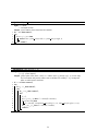
As discussed in Section 7, the main test data we use are derived from the relation Trains in the database
berlintest, containing 562 undergrund trains moving according to schedule on the network UBahn. The
schema of Trains is
Trains(Id: int, Line: int, Up: bool, Trip: mpoint)
where Id is a unique identifier for this train (trip), Line is the line number, Up indicates which direction
the train is going, and Trip contains the actual trajectory. We briefly look at these data within the system.
1. Start the S ECONDO kernel together with the graphical user interface. Open a shell and type
cd ˜secondo/bin
SecondoMonitor -s
[SecondoMonitor.exe -s on a Windows platform]
Open a new shell:
cd ˜secondo/Javagui
sgui
2. In the command window (top left), type
open database berlintest;
query UBahn
A pop-up window appears asking for a display style for the geoData attribute of the UBahn relation. Leave the default and click OK. The UBahn network appears in the viewer at the bottom.
3. In the File menu, select Load categories which makes some other display styles available. Choose
BerlinU.cat.
4. In S ECONDO , it is possible to type query plans directly, without the use of an optimizer. This is
what we do next. In the command window, type:
query Trains count
This confirms that relation Trains is present and has 562 tuples. Operator count is applied to the
Trains relation in postfix notation.
5. query Trains feed filter[.Trip present six30] consume
This selects trains whose Trip attribute is defined at 6:30 (six30 is a S ECONDO object of type
instant in the database). Here the feed operator (applied in postfix notation to Trains) creates a
stream of tuples. The filter operator passes only tuples to its output stream fulfilling a predicate.
Consume collects a stream of tuples into a relation which is then displayed at the user interface.
A pop-up window asks for the display style. From View Category select QueryMPoint. Standard
attributes appear in the text window at the left side of the Hoese viewer (the viewer forms the
bottom of the entire window). When you select one of the Trip attributes, also geometries appear
in the graphics window on the right.
6. Animate the displayed trains using the buttons at the top left of the viewer. The double arrow
buttons allow one to double or halve the speed of the animation.
This may suffice as a very brief introduction to using S ECONDO . To become a bit more acquainted
with the user interface and the querying and visualizing of moving objects, we recommend to go through
the brief ”Do it yourself demo” ([5], Section 2). More information about using S ECONDO can be found
at the Web site [8], in particular in the user manual [7].
26
8.1.5
Using knearest
On the small Trains relation it is feasible to run a TCkNN query using just the knearest operator which
implements the refine step as described in Section 6. We use the unit representation of Trains, a relation
called UnitTrains. It is present in the database, but could alse be created using the command:
let UnitTrains = Trains feed
projectextendstream[Id, Line, Up; UTrip: units(.Trip)] consume
The projectextendstream operator creates a stream of units from the Trip attribute of each input tuple
and outputs for each unit a copy of the original tuple restricted to attributes Id, Line, Up, and the new
unit attribute UTrip.
1. query UnitTrains count
Relation UnitTrains is present and has 51544 tuples.
2. We create a version of UnitTrains where units are ordered by start time:
let UTOrdered = UnitTrains feed
extend[Mintime: minimum(deftime(.UTrip))]
sortby[Mintime asc] consume
Operator extend adds derived attributes to tuples.
3. From the window showing displayed objects (top right), remove all items using the clear button.
Then display the UBahn network again as in step 2 of Section 8.1.4.
4. query Trains
This loads the entire set of trains into the user interface for display. It takes some time. Choose
display style QueryMPoint.
5. query train7
This loads a S ECONDO object of type mpoint which we will use as a query object. Display as
QueryPoint.
6. Find the five continuous nearest neighbors to train7.
query UTOrdered feed knearest[UTrip, train7, 5] consume
Arguments to the knearest operator are the ordered stream of unit tuples, the name of the attribute,
the query trajectory, and the number of neighbors. Choose QueryMPoint2 for display style. In the
animation, one can observe that always the five closest trains appear in blue (the result of this
query).
7. Find the five continuous nearest neighbors to train7 belonging to line 5.
query UTOrdered feed filter[.Line = 5]
knearest[UTrip, train7, 5] consume
This illustrates that nearest neighbors fulfilling additional conditions can be found.
8.1.6
Creating Test Data
We now show how the test data are generated. Here we restrict attention to the creation of data set
Trains25. This is done by running the script file createtrains25 from [4] which needs to be placed
in the secondo/bin directory. The file is explained in Appendix C.
Close down any running S ECONDO system. Open a new shell and type
SecondoTTYNT -i createtrains25
This creates appropriate versions of relations and indexes for the three algorithms.
27
8.1.7
Using the Three Algorithms CTkNN, HCNN, and HCkNN
Each of the three main algorithms compared in he experiments is available as an operator. They are called
knearestfilter and knearest , greeceknearest , and chinaknearest for CTkNN, HCNN, and HCTkNN,
respectively.
As a query object we use train742, which is the first train of line 7 within the field (4, 2) of the 5 x 5
pattern. The dataset considered now can be visualized by translating the underlying UBahn network in
the same way (see Appendix C for an explanation).
1. Create UBahn25 and visualize it:
let UBahn25 = UBahn feed five feed f1 five feed f2 product product
projectextend[Name, Typ;
geoData: .geoData translate[30000.0 * .no_f1, 30000.0 * .no_f2],
FieldX: .no_f1,
FieldY: .no_f2]
consume;
query UBahn25
As discussed in Section 7, the Trains25 dataset has about 1.3 million units. It is too large to load
it entirely into the viewer. To be able to interpret the answer of the query, we visualize the trains
moving in field (4, 2) together with the query object, train742.
2. Load trains from field (4, 2) and the query object.
query Trains25 feed filter[(.FieldX = 4) and (.FieldY = 2)] consume;
query train742
3. Find the 5 closest trains to train742 within data set Trains25, using TCkNN. We proceed in two
steps to display first the candidates found in the filter step, using operator knearestfilter , and then
the complete solution.
query UnitTrains25_UTrip UnitTrains25
UnitTrains25Cover_RecId UnitTrains25Cover
knearestfilter[UTrip, train742, 5] consume;
query UnitTrains25_UTrip UnitTrains25
UnitTrains25Cover_RecId UnitTrains25Cover
knearestfilter[UTrip, train742, 5]
knearest[UTrip, train742, 5] consume;
The arguments to knearestfilter are the R-tree index and the indexed relation, then the B-tree index
on the relation with coverage numbers and this relation, finally (in the square brackets) the attribute
name, the query trajectory, an the number k.
4. Find the 5 closest trains to train742 within data set Trains25, using HCNN.
query UTOrdered_RTreeBulk25 UTOrdered25
greeceknearest[UTrip, train742, 5] consume;
Arguments are the R-tree and the unit relation, clustered in the same way.
5. Find the 5 closest trains to train742 within data set Trains25, using HCkNN.
query UnitTrains_UTrip_tbtree25 UnitTrains25C
chinaknearest[UTrip, train742, 5] consume;
Arguments are the TB-tree and the unit relation. Here units are ordered by train objects.
28
8.2 Repeating the Experiments
Experiments can be repeated using the scripts provided at [4]. As a preparation, extract all the files from
this zip-archive and place them into the secondo/bin directory. Files for data generation should be
called, for example:
SecondoTTYNT -i createtrains25
Files for performing experiments should be called
SecondoTTYBDB -i query-k-trains25
As an example, Appendix D shows the script query-k-trains25 to run the experiment “performance vs. k” of Section 7.4.2. Note that the last queries examine S ECONDO relations SEC2COMMANDS
and SEC2COUNTERS. These system relations capture information about query execution; each command after starting a S ECONDO system is numbered sequentially. Hence after the first command for
opening the database, the ten queries for each of the three algorithms are numbered 2 through 11, 12
through 21, and 22 through 31, respectively. The queries aggregate over these executions to get average
CPU time and numbers of page accesses.
Results should roughly correspond to those displayed in Figure 17 and Tables 5 and 6. Of course,
only trends should agree; absolute numbers may differ due to the different platforms used.
9 Conclusions
In this paper we have studied continuous k nearest neighbor search on moving objects trajectories when
both query and data objects are mobile. We have presented a filter-and-refine approach. The main idea
in the filter step was to compute for each node of the index its time dependent coverage function in
preprocessing and to store a suitable simplification of this function. Coverage numbers are then essential
for pruning during the index traversal. This is further supported by the use of efficient data structures
to compute spatial bounding boxes of partial query trajectories and to keep track of node coverages and
node distances during traversal. The refinement step can also be used independently to find continuous k
nearest neighbors fulfilling further predicates. An experimental comparison shows that the new algorithm
outperforms the two competing algorithms in most cases by orders of magnitude.
As a second aspect, we have advocated a methodology of experimental research that makes data
structures and algorithms available in a system context and that publishes together with papers also
their implementation used in experiments. A platform has been provided that allows authors to publish
software in this way. As a benefit, readers can relatively easily repeat or extend the experiments presented
in the paper. Furthermore, in the long run, researchers will find existing implementations to compare
to instead of always reimplementing competing techniques from scratch. We have used the research
contribution of this paper as an example to demonstrate this style of publishing experimental research.
Open questions for future work are whether the pruning techniques of the filter step can be adapted to
other cases, for example other query types such as reverse nearest neighbors, network-based movement,
or the presence of additional predicates.
Acknowledgements
The contribution of Angelika Braese who implemented preliminary versions of both the filter and the
refinement algorithm in her bachelor thesis, is gratefully acknowledged.
29
References
[1] BerlinMOD. http:dna.fernuni-hagen.de/secondo/BerlinMOD.html.
[2] Nearest Neighbor Algebra Plugin. Included with submission.
http://dna.fernuni-hagen.de/Secondo.html/files/plugins/NN.zip.
[3] R-tree Portal. http:www.rtreeportal.org.
[4] Scripts to execute the experiments of this paper. Included with submission.
http://dna.fernuni-hagen.de/papers/KNN/knn-experiment-script.zip.
[5] Secondo. A Database System for Moving Objects.
http://dna.fernuni-hagen.de/Secondo.html/Secondo-mod.pdf.
[6] Secondo Plugins. http://dna.fernuni-hagen.de/Secondo.html/content plugins.html.
[7] Secondo User Manual. http://dna.fernuni-hagen.de/Secondo.html/files/SecondoManual.pdf.
[8] Secondo Web Site. http://dna.fernuni-hagen.de/Secondo.html/.
[9] R. Benetis, C. S. Jensen, G. Karciauskas, and S. Saltenis. Nearest and reverse nearest neighbor
queries for moving objects. VLDB J., 15(3):229–249, 2006.
[10] J. L. Bentley and T. Ottmann. Algorithms for reporting and counting geometric intersections. IEEE
Trans. Computers, 28(9):643–647, 1979.
[11] S. Berchtold, C. Böhm, and H.P. Kriegel. Improving the query performance of high-dimensional
index structures by bulk load operations. In EDBT, pages 216–230, 1998.
[12] J. Bercken, B. Seeger, and P. Widmayer. A generic approach to bulk loading multidimensional
index structures. In VLDB, pages 406–415, 1997.
[13] V. P. Chakka, A. Everspaugh, and J. M. Patel. Indexing large trajectory data sets with seti. In CIDR,
2003.
[14] M. de Berg, O. Cheong, M. van Kreveld, and M. Overmars. Computational Geometry: Algorithms
and Applications. Springer, Heidelberg, 3rd edition, 2008.
[15] C. Düntgen, T. Behr, and R.H. Güting. BerlinMOD: A benchmark for moving object databases.
The VLDB Journal, online first, 2009.
[16] L. Forlizzi, R. H. Güting, E. Nardelli, and M. Schneider. A data model and data structures for
moving objects databases. In SIGMOD, pages 319–330, 2000.
[17] E. Frentzos. Personal communication.
[18] E. Frentzos, K. Gratsias, N. Pelekis, and Y. Theodoridis. Algorithms for nearest neighbor search
on moving object trajectories. GeoInformatica, 11(2):159–193, 2007.
[19] E. Frentzos, K. Gratsias, and Y. Theodoridis. Index-based most similar trajectory search. In ICDE,
pages 816–825. IEEE, 2007.
[20] Y. Gao, C. Li, G. Chen, Q. Li, and C. Chen. Efficient algorithms for historical continuous k nn
query processing over moving object trajectories. In APWeb/WAIM, pages 188–199, 2007.
30
[21] Y. J. Gao, C. Li, G. C. Chen, L. Chen, X. T. Jiang, and C. Chen. Efficient k-nearest neighbor search
algorithms for historical moving object trajectories. Journal of Computer Science and Technology,
22(2):232–244, 2007.
[22] F. Giannotti and D. Pedreschi, editors. Mobility, Data Mining and Privacy - Geographic Knowledge
Discovery. Springer, 2008.
[23] J. Gudmundsson and M. J. van Kreveld. Computing longest duration flocks in trajectory data. In
Rolf A. de By and Silvia Nittel, editors, GIS, pages 35–42. ACM, 2006.
[24] R. H. Güting, M. H. Böhlen, M. Erwig, C. S. Jensen, N. A. Lorentzos, M. Schneider, and M. Vazirgiannis. A foundation for representing and quering moving objects. ACM TODS, 25(1):1–42,
2000.
[25] G. R. Hjaltason and H. Samet. Distance browsing in spatial databases. ACM Trans. Database Syst.,
24(2):265–318, 1999.
[26] Y. Huang, C. Chen, and C. Lee. Continous k-nearest neighbor query for moving objects with
uncertain velocity. Geoinformatica, 2007.
[27] G. S. Iwerks, H. Samet, and K. P. Smith. Continuous k-nearest neighbor queries for continuously
moving points with updates. In VLDB, pages 512–523, 2003.
[28] H. Jeung, M. L. Yiu, X. Zhou, C. S. Jensen, and H. T. Shen. Discovery of convoys in trajectory
databases. In VLDB, 2008.
[29] M. F. Mokbel, T. M. Ghanem, and W. G. Aref. Spatio-temporal access methods. IEEE Data Eng.
Bull., 26(2):40–49, 2003.
[30] G. M. Morton. A computer oriented geodetic data base and a new technique in file sequencing.
Technical report, IBM Ltd. Ottawa, 1966.
[31] K. Mouratidis, M. Hadjieleftheriou, and D. Papadias. Conceptual partitioning: An efficient method
for continuous nearest neighbor monitoring. In SIGMOD, pages 634–645, 2005.
[32] D. Pfoser, C. S. Jensen, and Y. Theodoridis. Novel approaches in query processing for moving
object trajectories. In VLDB, pages 395–406, 2000.
[33] K. Raptopoulou, A. Papadopoulos, and Y. Manolopoulos. Fast nearest-neighbor query processing
in moving-object databases. GeoInformatica, 7(2):113–137, 2003.
[34] S. Rasetic, J. Sander, J. Elding, and M. A. Nascimento. A trajectory splitting model for efficient
spatio-temporal indexing. In VLDB, 2005.
[35] N. Roussopoulos, S. Kelly, and F. Vincent. Nearest neighbor queries. In SIGMOD, 1995.
[36] A. P. Sistla, O. Wolfson, S. Chamberlain, and S. Dao. Modeling and querying moving objects. In
W. A. Gray and Per-Åke Larson, editors, Proceedings of the Thirteenth International Conference
on Data Engineering, April 7-11, 1997 Birmingham U.K, pages 422–432. IEEE Computer Society,
1997.
[37] Z. Song and N. Roussopoulos. K-nearest neighbor search for moving query point. In SSTD, pages
79–96, 2001.
[38] Y. Tao and D. Papadias. Time-parameterized queries in spatio-temporal databases. In SIGMOD,
pages 334–345, 2002.
31
[39] Y. Tao, D. Papadias, and Q. Shen. Continuous nearest neighbor search. In VLDB, pages 287–298,
2002.
[40] O. Wolfson, B. Xu, S. Chamberlain, and L. Jiang. Moving objects databases: Issues and solutions.
In SSDBM, pages 111–122, 1998.
[41] X. Xiong, M. F. Mokbel, and W. G. Aref. Sea-cnn: Scalable processing of continuous k-nearest
neighbor queries in spatio-temporal databases. In ICDE, pages 643–654, 2005.
[42] X. Yu, K. Q. Pu, and N. Koudas. Monitoring k-nearest neighbor queries over moving objects. In
ICDE, pages 631–642, 2005.
A
Implementation of the Cover Structure
A node has the following structure:
type node = record
time interval [t1 , t2 ];
pointer to node left, right;
list of cover entry list;
list of pairs <which, cover entry> startlist, endlist
end record.
The lists list, startlist, and endlist are doubly linked lists with elements of the form <pred, succ, pointer
to cover entry>. Whenever a cover entry is added to such a list, actually a pointer to the cover entry is
inserted and at the same time a pointer to this list element is added to the list refs in the cover entry. In
this way efficient deletion of cover entries is possible.
Update methods are insert entry, add coordinate, insert interval, and delete entry. Query methods
are point query and range query.
Algorithm 9: insert entry(ce)
Input: ce - a cover entry;
Output: none
1 let root = this.root();
2 add coordinate(root, ce.t1 , true, ce);
3 add coordinate(root, ce.t2 , false, ce);
4 insert interval(root, ce.t1 , ce.t2 , ce);
32
Algorithm 10: add coordinate(n, t, start, ce)
Input: n - a node;
t - an instant of time;
start - a boolean indicating whether a left or right end is added;
ce - a cover entry.
Output: none
/* modifies the segment tree to accomodate a possibly new
coordinate t and adds the entry as either a start or an end
entry.
*/
1 if n is a leaf then
2
if n.t1 < t < n.t2 then
3
n.left = new node(n.t1 , t);
4
n.right = new node(t, n.t2 );
5
if start then n.right.startlist.append(<bottom, ce>);
6
else n.left.endlist.append(<top, ce>);
7
8
9
10
11
12
13
else // n is an inner node
if t = n.left.t2 then
if start then n.right.startlist.append(<bottom, ce>);
else n.left.endlist.append(<top, ce>);
else
if t < n.left.t2 then add coordinate(n.left, t, start, ce);
else add coordinate(n.right, t, start, ce);
14
Algorithm 11: insert interval(n, t1 , t2 ,ce)
Input: n - a node;
[t1 , t2 ] - a time interval;
ce - a cover entry;
Output: none
1 if [n.t1 , n.t2 ] ⊆ [t1 , t2 ] then n.list.append(ce);
2 if n is an inner node then
3
if t1 < n.left.t2 then insert interval(n.left, t1 , t2 , ce);
4
if t2 > n.right.t1 then insert interval(n.right, t1 , t2 , ce);
Algorithm 12: delete entry(ce)
Input: ce - a cover entry
Output: none
1 for each s ∈ ce.refs do remove(s);
33
Algorithm 13: point query(n, t)
Input: n - a node;
t - an instant of time.
Output: a set of entries whose time intervals contain t.
1 if n = null then return ∅;
2 else
3
if n.t1 ≤ t ≤ n.t2 then
4
return n.list ∪ point query(n.left, t) ∪ point query(n.right, t);
5
else return ∅;
Algorithm 14: range query(n, t1 , t2 )
Input: n - a node;
[t1 , t2 ] - a time interval.
Output: a list of pairs of the form <which, ce> where which ∈ {bottom, top}, ce a cover entry.
The list contains only entries whose start or end time lies within [t1 , t2 ], in temporal
order w.r.t their start or end time.
1 if n = null then return ∅;
2 else
3
if n.t2 < t1 then return ∅;
4
else
5
if t2 < n.t1 then return ∅;
6
else
7
S = ∅;
8
if t1 ≤ n.t1 ≤ t2 then S = concat(S, n.startlist);
9
if n is not a leaf then
10
S = concat(S, concat(range query(n.left, t1 , t2 ), range query(n.right, t1 , t2 )));
11
12
if t1 ≤ n.t2 ≤ t2 then S = concat(S, n.endlist);
return S;
34
B Tables for Experimental Evaluation
Tables 3 through 13 provide the numeric results of the experiments of Section 7.
Datasize(million)
TCkNN
HCTkNN
HCNN-Bulk
HCNN-Standard
0.051
0.2125
3.93
0.86
2.373
0.464
0.359
6.8483
4.088
217.441
1.29
0.639
12.014
11.516
972.924
3.3
0.99
13.146
24.283
5.154
4.419
13.453
36.017
Table 3: CPU time for datasize (sec)
Datasize(million)
TCkNN
HCTkNN
HCNN-Bulk
HCNN-Standard
0.051
2.9915
11.229
26.8733
23.551
0.464
2.833
42.836
98.0624
84.0161
1.29
4.5534
52.4031
280.0883
193.1001
3.3
6.4553
58.5742
606.3243
5.154
10.6509
58.6521
910.9049
Table 4: I/O for datasize (x103 )
k
TCkNN
HCTkNN
HCNN
1
0.501
1.48
7.523
5
0.657
11.916
10.68
10
0.825
57.845
15.584
20
1.172
274.365
31.114
Table 5: CPU time for k on Trains25 (sec)
35
50
2.177
1614
134.84
k
TCkNN
HCTkNN
HCNN
1
2.8771
29.6357
237.2368
5
4.6123
54.1393
262.0703
10
6.1454
92.6692
291.7257
20
8.875
181.0361
352.9404
50
15.3727
456.130
648.211
Table 6: I/O for k on Trains25 (x103 )
k
TCkNN
HCTkNN
HCNN
1
0.431
1.046
0.987
5
1.01
56.41
7.579
10
1.206
125.284
25.886
20
1.643
280.566
66.211
50
1.761
638.712
85.5
Table 7: CPU time for k on Trucks (sec)
k
TCkNN
HCTkNN
HCNN
1
2.2023
11.6411
22.8143
5
7.848
71.3964
75.6934
10
10.63
129.4408
138.7414
20
14.5099
268.7456
249.2896
50
15.648
432.0422
442.215
Table 8: I/O for k on Trucks (x103 )
Qt
TCkNN
HCTkNN
HCNN
0.05
0.202
0.083
0.296
0.1
0.311
0.146
1.102
0.2
0.359
0.302
1.832
0.5
0.659
0.78
4.648
1.0
0.64
13.397
10.549
Table 9: CPU time for Qt on Trains25 (sec)
Qt
TCkNN
HCTkNN
HCNN
0.05
1.4296
1.8493
10.4061
0.1
1.3461
3.5507
31.1233
0.2
2.6451
7.3944
53.3972
0.5
3.6089
17.0242
127.1772
1.0
4.5706
55.7424
262.0703
Table 10: I/O for Qt on Trains25 (x103 )
Qt
TCkNN
HCTkNN
HCNN-Bulk
HCNN-Standard
0.05
0.049
0.057
0.142
0.146
0.1
0.086
0.19
0.393
0.454
0.2
0.122
0.302
0.741
0.933
0.5
0.255
1.446
1.428
2.308
Table 11: CPU time for Qt on Trucks (sec)
36
1.0
0.865
56.244
7.556
18.585
Qt
TCkNN
HCTkNN
HCNN-Bulk
HCNN-Standard
0.05
0.5164
1.292
3.5888
3.0866
0.1
0.8069
4.0847
7.855
6.3347
0.2
1.2285
6.4763
14.3979
11.0045
0.5
2.4016
16.5545
28.2744
22.0227
1.0
6.8346
67.5294
75.6943
58.6015
Table 12: I/O for Qt on Trucks (x103 )
number of units
TCkNN
HCTkNN
HCNN
100
0.3
0.483
2.222
200
0.932
2.548
7.401
500
2.695
73.768
20.364
800
5.067
1504.91
45.664
1000
4.825
1635.61
50.83
Table 13: CPU time for long trajectory (sec)
number of units
TCkNN
HCTkNN
HCNN
100
2.4784
10.2999
51.9219
200
5.9583
30.7703
141.5523
500
14.1228
155.9528
388.4074
800
24.1902
416.571
783.7167
Table 14: I/O for long trajectory (x103 )
37
1000
24.6388
511.098
855.2416
C
Creation of Test Data
This is a commented version of file createtrains25.
This script creates the Trains25 data set for each of the three algorithms TCkNN, HCNN, and
HCTkNN. Starting point is the relation Trains containing 562 undergrund trains moving according to
schedule on the network UBahn. We now explain the commands in the script.
let five = ten feed filter[.no < 6] consume;
let Trains25 = Trains feed five feed f1 five feed f2
product product
projectextend[Id, Line, Up;
Trip: .Trip translate[[const duration value (0 0)],
30000.0 * .no_f1, 30000.0 * .no_f2],
FieldX: .no_f1,
FieldY: .no_f2]
consume;
The first command creates a relation five containing the numbers 1 through 5. It is used to make 25 copies
of the Trains in the next command, using two product operator calls to build the Cartesian product of
Trains and two instances of relation five. Note that operations are often applied in postfix notation. Next
the projectextend operator performs a projection on each tuple, keeping attributes Id, Line, and Up. It
als adds new attributes to the tuple whose values are computed from existing attributes. Attribute Trip is
derived from the original Trip attribute by translating the geometry in the (x, y, t) space. The temporal
shift is 0, hence all copies of the trains move at the same time as their originals. However, spatially,
geometries are shifted by distance no f 1 * 30000 in x-direction and by distance no f 2 * 30000 in ydirection. Here no f 1 and no f 2 come from the two instances of the five relation. Hence 25 copies are
made of each train arranged in a 5 x 5 grid. The field indices in the grid are also kept in the tuple as
FieldX and FieldY. The last operation consume collects the stream of tuples into a relation.
let train742 = Trains25 feed
filter[(.Line = 7) and (.FieldX = 4) and (.FieldY = 2)]
extract[Trip];
let train123 = Trains25 feed
filter[(.Line = 1) and (.FieldX = 2) and (.FieldY = 3)] extract[Trip];
...
Next ten query trains are selected from the new Trains25 relation. The extract operation gets the value
of attribute Trip from the first tuple of its input stream. Hence train742 is now an object of type mpoint,
i.e., a trajectory.
As explained in Section 5.3, we partition the 3D space into small spatiotemporal cells such that each
cell contains on the average enough units to fill about r nodes of an R-tree. The original Trains relation
fits spatially into a box of size 30000 x 20000, with lower left corner at position (-3600, 1200). Copies
are moved by multiples of 30000 as shown above. We now impose a grid with cells of size 10000 x
10000 spatially, and 5 minutes temporally. The calculation leading to these sizes is the following. One
can observe that in the original Trains relation at any instant of time on the average 90 trains are present.
We aim to have about p = 15 objects present within each spatial cell, hence form a grid of 6 cells. This
defines the cell size of 10000 x 10000 for the original Trains relation. The relation has 51444 units. An
R-tree node can take about 60 entries in our implementation; hence to fill about r = 5 nodes, about 300
units should be in a spatiotemporal cell. Assuming units are uniformly distributed in space and time,
51444 / (6 * 300) = 28.58 means that the temporal extent should be split into roughly 30 parts. As the
temporal extent of the trains relation is about 2.5 hours, the duration of each part should be about 5
38
minutes. The larger relation Trains25 will use the same temporal partitioning; the spatial grid cells of
size 10000 x 10000 are effectively translated in the same way as the Trains.
let six00 = theInstant(2003,11,20,6);
let minutes5 = [const duration value (0 300000)];
To introduce the temporal partition of the 3D space, we define the instant 6am and a duration of 5 minutes
(300000 ms).
let UnitTrains25 = Trains25 feed
projectextendstream[Id, Line, Up; UTrip: units(.Trip)]
addcounter[No, 1]
extend[
Temp: (minimum(deftime(.UTrip)) - six00) / minutes5,
CellX: real2int((minD(bbox2d(.UTrip), 1) + 3600.0) / 10000.0),
CellY: real2int((minD(bbox2d(.UTrip), 2) - 1200.0) / 10000.0)]
sortby[Temp asc, CellX asc, CellY asc, UTrip asc]
remove[Temp, CellX, CellY]
consume;
The projectextendstream operator creates a stream of units from the Trip attribute of each input tuple
and outputs for each unit a copy of the original tuple restricted to attributes Id, Line, Up, and the new
unit attribute UTrip. Then addcounter adds an attribute No with a running number to the current tuple.
The extend operator computes integer indices Temp, CellX, and CellY according to the 3D partition
explained above for a given unit, accessing its geometry. The resulting stream of tuples is sorted first by
the three indices of a spatiotemporal cell, and finally by UTrip (which in effect is the start time of the
unit). After sorting, the indices needed for sorting can be removed again before storing the relation.
let UnitTrains25_UTrip = UnitTrains25 feed addid bulkloadrtree[UTrip];
The R-tree is created by bulkload. The order in the underlying relation is the same as that used in the
bulkload; hence a clustering effect is achieved.
let UnitTrains25Cover = coverage(UnitTrains25_UTrip) consume;
The coverage operator traverses the R-tree, computing the coverage function and from it the three coverage numbers resulting from the hat operation (Section 5.3.1). They are entered into relation UnitTrains25Cover.
let UnitTrains25Cover_RecId = UnitTrains25Cover createbtree[RecId];
The relation with coverage numbers is indexed. This completes data generation for our algorithm
TCkNN. Next test data for HCNN are generated.
let UTOrdered25 = UnitTrains25 feed sortby[UTrip asc] consume;
let UTOrdered_RTreeBulk25 = UTOrdered25 feed addid
bulkloadrtree[UTrip];
The UnitTrains25 are ordered by units and stored in this order. This is essentially an order on the start
times of units. The index is then built by bulkload on the temporally ordered stream of tuples. Again the
index is clustered like the relation. As discussed in Section 7, this version of HCNN is the most efficient
one.
let UnitTrains25C = Trains25 feed
projectextendstream[Id, Line, Up;
addcounter[No, 1] consume
UTrip: units(.Trip)]
let UnitTrains_UTrip_tbtree25 = UnitTrains25C feed addid
bulkloadtbtree[Id, UTrip, TID];
39
Finally, for HCTkNN the UnitTrains25 relation must be in the order of Train objects. Then the TB-tree
index is built by bulkload.
D
Queries on Trains 25, varying k
This is a shortened version of file query-k-trains25.
open database berlintest;
#for different number of neighbors requested, change the value of k
#Germany
query
UnitTrains25_UTrip UnitTrains25
knearestfilter[UTrip, train742,
query
UnitTrains25_UTrip UnitTrains25
knearestfilter[UTrip, train523,
... (10 queries in total)
UnitTrains25Cover_RecId UnitTrains25Cover
5] knearest[UTrip,train742, 5] count;
UnitTrains25Cover_RecId UnitTrains25Cover
5] knearest[UTrip,train523, 5] count;
# Greece Bulk
query UTOrdered_RTreeBulk25 UTOrdered25 greeceknearest[UTrip,train742, 5]
count;
query UTOrdered_RTreeBulk25 UTOrdered25 greeceknearest[UTrip,train523, 5]
count;
... (10 queries in total)
#China
query UnitTrains_UTrip_tbtree25 UnitTrains25 chinaknearest[UTrip,train742,5]
count;
query UnitTrains_UTrip_tbtree25 UnitTrains25 chinaknearest[UTrip,train523,5]
count;
... (10 queries in total)
# Results Germany
query SEC2COMMANDS feed filter[(.CmdNr >= 2) and (.CmdNr <= 11)]
avg[CpuTime];
query SEC2COUNTERS feed filter[.CtrStr = "SmiRecord::Read:Calls"]
filter[(.CtrNr >= 2) and (.CtrNr <= 11)] avg[Value];
# Results Greece Bulk
query SEC2COMMANDS feed filter[(.CmdNr >= 12) and (.CmdNr <= 21)]
avg[CpuTime];
query SEC2COUNTERS feed filter[.CtrStr = "SmiRecord::Read:Calls"]
filter[(.CtrNr >= 12) and (.CtrNr <= 21)] avg[Value];
# Results China
query SEC2COMMANDS feed filter[(.CmdNr >= 22) and (.CmdNr <= 31)]
avg[CpuTime];
query SEC2COUNTERS feed filter[.CtrStr = "SmiRecord::Read:Calls"]
filter[(.CtrNr >= 32) and (.CtrNr <= 41)] avg[Value];
close database;
40
Verzeichnis der zuletzt erschienenen Informatik-Berichte
[336] Kunze, C., Lemnitzer,L., Osswald, R. (eds.):
GLDV-2007 Workshop - Lexical-Semantic and Ontological Resources
[337] Scheben, U.:
Simplifying and Unifying Composition for Industrial Models
[338] Dillhage, R., Grubba, T., Sorbi, A., Weihrauch, K., Zhong, N.:
CCA 2007 – Fourth International Conference on Computability and Complexity in
Analysis
[339] Beierle, Chr., Kern-Isberner, G. (Eds.): Dynamics of Knowledge and Belief Workshop at the 30th Annual German Conference on Artificial Intelligence, KI2007
[340] Düntgen, Chr., Behr, Th., Güting R. H.: BerlinMOD: A Benchmark for Moving Object
Databases
[341] Saatz, I.: Unterstützung des didaktisch-methodischen Designs durch einen
Softwareassistenten im e-Learning
[342] Hönig, C. U.:
Optimales Task-Graph-Scheduling für homogene und heterogene Zielsysteme
[343] Güting, R. H.:
Operator-Based Query Progress Estimation
[344] Behr, Th., Güting R. H.:
User Defined Topological Predicates in Database Systems
[345] vor der Brück, T.; Helbig, H.; Leveling, J.:
The Readability Checker Delite Technical Report
[346] vor der Brück:
Application of Machine Learning Algorithms for Automatic Knowledge Acquisition
and Readability Analysis Technical Report
[347] Fechner, B.:
Dynamische Fehlererkennungs- und –behebungsmechanismen für verlässliche
Mikroprozessoren
[348] Brattka, V., Dillhage, R., Grubba, T., Klutsch, Angela.:
CCA 2008 - Fifth International Conference on Computability and Complexity in
Analysis
[349] Osterloh, A.:
A Lower Bound for Oblivious Dimensional Routing
[350] Osterloh, A., Keller, J.:
Das GCA-Modell im Vergleich zum PRAM-Modell
[351] Fechner, B.:
GPUs for Dependability