Download An Edge Quadtree for External Memory

An Edge Quadtree for External Memory
Herman Haverkort1 and Mark McGranaghan2? and Laura Toma2??
1
Eindhoven University of Technology, the Netherlands
2
Bowdoin College, USA
Abstract. We consider the problem of building a quadtree subdivision
for a set E of n non-intersecting edges in the plane. Our approach is to
first build a quadtree on the vertices corresponding to the endpoints of
the edges, and then compute the intersections between E and the cells
in the subdivision. For any k ≥ 1, we call a K-quadtree a linear compressed quadtree that has O(n/k) cells with O(k) vertices each, where
each cell stores the edges intersecting the cell. We show how to build a
K-quadtree in O(sort(n + l)) i/o’s, where l = O(n2 /k) is the number
of such intersections. The value of k can be chosen to trade off between
the number of cells and the size of a cell in the quadtree. We give an
empirical evaluation in external memory on triangulated terrains and
USA TIGER data. As an application, we consider the problem of map
overlay, or finding the pairwise intersections between two sets of edges.
Our findings confirm that the K-quadtree is viable for these types of data
and its construction is scalable to hundreds of millions of edges.
1
Introduction
The word quadtree describes a class of data structures that partition the space
hierarchically and are defined by a stopping criterion that decides when a region
is not subdivided further. In 2D, the quadtree recursively divides a square containing the data into four equal regions (quadrants or cells), until each region
satisfies the stopping condition (usually, when a cell is “small” enough). The
set of cells that are not split further define the leaves of the tree and represent
a subdivision of the input region. Quadtrees have been used for many types
of data (points, line segments, polygons, rectangles, curves) and many types of
applications. For an ample survey we refer to [12].
In this paper we are interested in quadtrees for data sets that are so large
that they do not fit in the internal memory of the computer, so that at any time,
most of the data has to reside in external memory. To analyze the efficiency of
the construction and query algorithms in this case, we use the standard i/omodel by Aggarwal and Vitter [2]. In this model, a computer has an internal
memory of size M and an arbitrarily large disk. The data is stored on disk in
blocks of size B, and, whenever the algorithms needs to access data not present in
memory, it loads the block(s) containing the data from disk. The i/o-complexity
?
??
Supported by Bowdoin Freedman Fellowship and NSF award no. 0728780.
Supported by NSF award no. 0728780.
of an algorithm is the number of i/o’s it performs, that is, the number of blocks
transferred (read or written) between main memory and disk. Sorting takes
n
n
sort(n) = Θ( B
logM/B B
) i/o’s [2]; scanning takes scan(n) = Θ(n/B) i/o’s.
Quadtrees can be viewed as trees representing the hierarchical space decomposition, or as the set of leaf cells ordered along a space-filling curve. The
latter variant of quadtree, called the linear quadtree, was introduced by Gargantini [5]. The linear quadtree is particularly useful when dealing with disk-based
structures, because its space requirements are smaller. Quadtrees are known to
perform well empirically in many different applications, but their worst-case behaviour is not ideal, except in the simplest cases. Given a set of n points in the
plane, a quadtree that splits a region until it contains at most one point can have
unbounded size. However, it is known how to construct a compressed quadtree of
O(n) cells which each have at most one point. In a compressed quadtree, paths
consisting of nodes with only one non-empty child are replaced by a single node,
with all empty children merged into one. Throughout this paper, the concept of
quadtrees will encompass both compressed and uncompressed quadtrees.
Building a quadtree on a set of n non-intersecting edges in the plane, rather
than points, is harder. We refer to a quadtree for a set of edges as an edge
quadtree, and we denote by l the number of intersections between the edges and
the cells in the quadtree subdivision. One way to build an edge quadtree is to
first build a compressed quadtree on the endpoints of the edges, and then compute the intersections between the edges and the cells in the subdivision. In the
worst case, each edge can intersect almost all cells, giving a quadtree of quadratic
size. Another type of edge quadtree may split a region until it intersects a single
edge. Since the distance between two edges can be arbitrarily small, the resulting
quadtree has unbounded size. Other edge quadtrees can be defined by formulating specific stopping criteria. Such structures were described by Samet et al. [14,
13, 10]. The PM quadtree [14] allows a region to contain more than one edge if the
edges meet at a vertex inside the region. Variants of PM quadtrees differ in how
to handle regions that contain no vertices. The segment quadtree [13] is a linear
quadtree in which a leaf cell is either empty, contains one edge and no vertices,
or contains precisely one vertex and its incident edges. The PMR quadtree [10]
is a linear quadtree where each region may have a variable number of segments
and regions are split if they contain more than a predetermined threshold. Hoel
and Samet [9] compared the PMR quadtree with some variants of R-trees on
TIGER data, in terms of storage requirements, construction time (disk i/o’s),
and a number of queries. They find that the PMR quadtree performs well compared to the R-tree for map overlay. Subsequently, improved algorithms for the
construction of the PMR quadtree have been proposed [7, 6, 8]. The algorithms
perform well in practice, but there are several disadvantages: First, the stopping
rule of the PMR quadtree means that the size of a leaf depends on both the
splitting threshold and the depth of the leaf, and the quadtree depends on the
insertion order. Second, the complexity is analysed in terms of various parameters that depend on the data, in a way that is not well understood. Finally, the
algorithms are fairly complex, and the performance is not worst-case optimal.
Quadtrees in the i/o-model were described by Agarwal et al. [1] and De
Berg et al. [4]. Agarwal et al. describe an algorithm for constructing a quadtree
on a set of n vertices in the plane such that each cell contains O(k) vertices
n
h
(for any k ≥ 1), that runs in O( B
log M/B ) i/o’s, where h is the height of the
quadtree. This is O(sort(n)) i/o’s when h = O(log n) i.e. the vertices are nicely
distributed. Their algorithm was implemented and tested in practice as part of
an application to interpolate LIDAR datasets into grids. De Berg et al. described
the star-quadtree for triangulations, and the guard-quadtree for sets of edges in
the plane, which contain at most one vertex per cell and can be constructed in
O(sort(n + l)) i/o’s, where l = O(n2 ) is the number of edge-cell intersections.
The star- and guard-quadtrees are designed to exploit fatness and density: for fat
triangulations3 and sets of edges of low density4 , respectively, the star-quadtree
and guard-quadtree have the property that each cell intersects O(1) edges, thus
l = O(n). An experimental evaluation of these structures has not been reported.
Our Contribution. We consider building an edge quadtree for a set E of
n non-intersecting edges. Let k ≥ 1 be a user defined parameter. Our algorithm
has two steps: First it builds, in O(sort(n)) i/o’s, a compressed linear quadtree
on the endpoints of E with O(n/k) cells in total and such that each cell has
O(k) vertices. Second, it computes the intersections between the edges and the
quadtree subdivision in O(sort(n + l)) i/o’s (where l = O(n2 /k) is the total
number of intersections). We refer to the resulting quadtree as a K-quadtree.
The first step, constructing the quadtree subdivision, is a generalization of
the algorithm for building guard-quadtrees in [4]. Compared to the algorithm
by Agarwal et al. [1], our algorithm has better complexity, is much simpler, and
gives an upper bound on the number of cells in the subdivision. The second step,
which we refer to as edge distribution, is based on an idea communicated to us
by Doron Nussbaum. For k = 1 the algorithm has the same complexity as in [4],
but it is simpler and faster.
In Section 4 we give an empirical evaluation of K-quadtrees on triangulated
terrains (in GIS: TINs) and USA TIGER data. We examine the size of the
quadtree, the size of a cell and the construction time for different values of k.
We use test datasets up to 427 million edges, two orders of magnitude larger than
in related work [7, 6, 8]. On TINs and TIGER data the K-quadtrees have linear
size, which matches the results of [9, 7, 6, 8]. In terms of construction time (or
bulk loading), a comparison with previous work is difficult. The running times
in [9] are given in terms of disk block accesses, not the total execution time. The
tests in [7, 6, 8] are performed on three TIGER data sets, the largest one having
approx. 200, 000 edges, on a machine with 64MB RAM. Our largest TIGER
bundle has 427 million edges (6.8 GB), and we use machines with 512MB RAM.
Furthermore a precise comparison is not possible without knowing all the tuning
parameters used in [8].
3
4
A triangulation such that every angle is larger than some fixed positive constant δ
Any disk D is intersected by at most λ edges whose length is at least the diameter
of D, for some fixed constant λ.
As an application of quadtrees we consider one of the basic operations in
GIS and spatial data structures, map overlay: computing the pairwise segment
intersections (overlay) between two sets of edges. Given two sets of edges, each
pre-processed as a quadtree, their intersections can be computed in a very simple
manner by scanning the two quadtrees as in [4]. We implemented map overlay
and report on the running time using various values of k.
Overall, our experimental results confirm that the K-quadtree is viable for
very large TIN and TIGER data. These represent relatively simple classes of
inputs; however they arise frequently in practice and have been used extensively
as tests beds for spatial index structures. Further experiments are necessary for
other types of data, and we leave this as a topic for future work.
2
Preliminaries
For simplicity, we assume that the edges E lie in the unit square. For quadtree
background and notation see e.g. [11, 4]. A square that is obtained by recursively
dividing the input square into quadrants is called a canonical square. To order
the quadrants, we use the z-order space-filling curve that visits the 4 quadrants,
recursively, in order SW, NW, SE, NE. z-order gives a well-defined ordering
between the cells in the quadtree subdivision, as well as between any two points.
For a point p = (px , py ) in the unit square, define its z-index Z(p) to be the value
in the range [0, 1) obtained by interleaving the bits in the fractional parts of px
and py . The value Z(p) is sometimes called the Morton block index of p. The
z-order of two points is the order of their z-indices. The z-indices of all points in
a canonical square σ form an interval [z1 , z2 ) of [0, 1), where z1 is the z-index of
the bottom left corner of σ. A compressed quadtree subdivision has two types of
cells: canonical squares, and donut cells, corresponding to empty nodes that were
merged together. A donut cell is the difference between two canonicalSsquares
[z1 , z2 ] − [z3 , z4 ] and is represented as the union of two intervals [z1 , z3 ] [z4 , z2 ].
With this notation, a (compressed) quadtree subdivision corresponds to a
subdivision Q of the z-order curve, and it can be viewed as a set of consecutive, adjacent, non-overlapping intervals, covering [0, 1), in z-order: Q = {[z1 =
0, z2 ), [z2 , z3 ), [z3 , z4 ), ...}; Each interval corresponds to a cell σi , which is either
a canonical square or a part of a donut. We represent a K-quadtree as a subdivision of the z-order curve where each intersection of an edge e with a cell σ
corresponding to the interval [z1 , z2 ) is represented by storing edge e with key
z1 . A K-quadtree is thus a list of pairs {(z1 , e)}, stored in order of z1 .
In the rest of the paper we denote by l the number of intersections between
E and the cells in the quadtree subdivision, and we use the terms quadtree,
quadtree subdivision and subdivision interchangeably.
3
Constructing a K-quadtree
In this section we describe our algorithm for building a K-quadtree. Let k ≥ 1
be a user defined parameter. Our algorithm has two steps: In the first step
it ignores the edges and builds, in O(sort(n)) i/o’s, a linear quadtree on the
endpoints of the edges. The quadtree has O(n/k) cells in total, each containing
O(k) vertices. Second, it computes the intersections between the edges and the
quadtree subdivision in O(sort(n + l)) i/o’s. We describe the two steps below.
Constructing the subdivision. Let P = {p0 , p1 , p2 , ...} be the vertices of E. A
straightforward idea to build a quadtree with O(k) vertices per cell would be
to start with one of the standard algorithms for building a quadtree with at
most one vertex per cell, and then traverse the subdivision and merge cells
into cells of size O(k). However, we would like to avoid generating first a larger
subdivision and then merging its cells to get a smaller subdivision. Another
approach might be to build the quadtree top-down: stop if the cell contains
O(k) vertices, otherwise split the cell and distribute the points among the four
children, and continue on the children recursively; however, this may take Θ(n2 )
time as the quadtree may have height Θ(n).
Our idea to generate a quadtree subdivision with O(n/k) cells and O(k)
vertices in each cell directly, is a simple and elegant generalization of an algorithm
in [4]. Assume that P has been sorted in z-order, and denote Pk the set of every
k th point in P: Pk = {p0 , pk , p2k , ...} ⊂ P. The idea is to build the quadtree
subdivision induced by Pk : for every pair of consecutive points in Pk , we find
their smallest enclosing canonical square, and output the z-indices corresponding
to the 4 z-intervals of the quadrants of this square. We claim that:
Lemma 1. The resulting list of z-indices represents a compressed quadtree subdivision with O(n/k) cells and O(k) vertices per cell.
Proof. Every pair of consecutive points of Pk causes a split, and generates 4
cells, therefore O(n/k) cells; each cell contains at most one point of Pk inside
(or otherwise it would have been split), therefore O(k) points of P.
Assuming that the operations involving z-indices take O(1) time, this step
runs in O(n) time and O(scan(n)) i/o’s. With the help of the stack described
in the appendix of [4], we can actually output the z-indices in increasing order
without additional i/o. Thus we get a compressed quadtree subdivision represented by a list of z-intervals, in z-order of their first endpoint: Q = {[z1 =
0, z2 ], [z2 , z3 ], ...} = {I1 , I2 , ...}. We note that in practice we represent the second
endpoint of the intervals implictly.
An algorithm for edge distribution when k = 1. Let Q = {I1 , I2 , ...} be a subdivision of the endpoints of E obtained by the algorithm described above, and
assume Q is given in z-order. We will now first consider the case k = 1, i.e.
every cell contains at most one vertex, and the total number of cells is O(n). We
describe how to find the intersections between Q and E in O(sort(n + l)) i/o’s.
Later we will show how to generalize this process to a subdivision with O(k)
vertices in a cell, where k > 1.
We assume edges are oriented from left to right, vertical segments are oriented
upwards, and let E+ and E− denote the edges of positive and negative slope,
respectively. The crux of the algorithm is to process the edges of positive and
negative slope separately. We describe below the two steps.
4
6
3
5
8
14
16
4
6
3
5
8
11 13
2
7
1
14
16
4
6
3
5
8
11 13
15
10 12
9
2
7
1
14
16
4
6
3
5
8
11 13
15
10 12
9
2
7
1
14
16
11 13
15
10 12
9
2
7
15
10 12
1
9
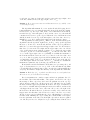
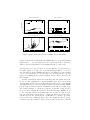
Fig. 1. (a) E+ (b) B7 (c) X7 and processing cell σ7 (d) X8
Distributing the edges of positive slope. The idea is to scan Q, one interval
at a time, and find all the edges in E+ intersecting the cell corresponding to
the current interval. Let Ij = [zj , zj+1 ] be the next interval we read from Q,
and let σj be the corresponding cell in the subdivision. There are two types of
intersections between σj and E+ , see Fig. 1:
– First, there may be edges that intersect σj and originate in σj ;
– Second, there may be edges that intersect σj and originate outside σj .
Intersections of the first type can be detected by scanning Q and E+ in sync,
as follows. Let E+ be sorted in z-order of the first endpoints of the edges. Let
Ij be the current interval in Q, and let e = (p, q) be the next edge in E+ . To
check whether e originates in σj means checking if z(p) ∈ Ij . This leads to the
following algorithm: For each interval Ij ∈ Q, we read from E+ all the edges
that originate in σj , and stop when encountering the first edge e0 = (p0 , q 0 ) with
z(p0 ) > zj+1 . Then we continue with the next interval from Q, in the same
fashion. Because the edges in E+ are stored in z-order of their first endpoint,
we know that once we encounter an edge with z(p0 ) > zj+1 , then all subsequent
edges have the same property and none of them can originate in σj . This runs
in O(scan(|Q| + |E+ |)) = O(scan(n)) i/o’s.
The harder problem is finding the intersections of σj with the edges that
originate outside σj . It is here that we exploit that E+ and E− are processed
separately. The key observation is that any edge of positive slope that intersects
σj originates in a cell that comes before σj , in z-order. In general we have:
Lemma 2. An edge of positive slope intersects the cells in Q in z-order.
Consider the current interval Ij in Q. By Lemma 2 it follows that all the
edges that intersect σj and do not start in σj must originate in a cell σi before
σj , S
that is i < j. Let Bj denote the S
boundary between the cells explored before
σj , i<j σi and the rest of the cells i≥j σi , for any j ≥ 1. The edges in E+ that
originate (but do not end) in a cell before σj will intersect the boundary Bj ; let
Xj be the set of these edges. See Fig. 1. More precisely, let XLj be the edges
of Xj that intersect Bj between the left edge of the unit square and the lower
left corner of σj , and let XB j be the edges of Xj that intersect Bj between the
lower left corner of σj and the bottom edge of the unit square. Here, if σj is the
second part of a donut, we define its lower left corner as the upper right corner
of the hole, which is, in fact, the upper right corner of σj−1 .
Lemma 3. Bj is a monotone staircase and the intersection of σj and Bj covers
a connected part of Bj .
The algorithm will maintain Xj on two stacks SL and SB , keeping the following invariant: before processing an interval Ij from Q, the stack SL contains,
from bottom to top, the edges of XLj in the order of their intersections with Bj
from the left edge of the unit square to the lower left corner of σj ; the stack SB
contains, from bottom to top, the edges of XB j in the order of their intersections
with Bj from the bottom edge of the unit square to the lower left corner of σj .
Initially, for j = 1, the boundary B1 is empty and both stacks are empty.
The algorithm now scans Q and E+ . When Ij is the next interval in Q, the
algorithm reads all edges that originate in σj from E+ , and pops all edges that
intersect σj “from before” from SL and SB . Out of these edges, we push those
that leave σj between the upper left and upper right corner onto SL, and those
that leave σj between the lower right and the upper right corner onto SB , in
order of their intersections with the boundary of σj towards the upper right
corner (if σj is part of a donut surrounding σj+1 , we take the lower left corner
of σj+1 as the upper right corner of σj ). Finally we establish the invariant for
the next interval: if the lower left corner of σj+1 lies above the lower left corner
of σj , we do this by popping edges from SL and pushing them onto SB one by
one until SL is empty or the top of SL intersects Bj+1 between the left edge
of the unit square and the lower left corner of σj+1 ; otherwise we establish the
invariant in a symmetric way by moving edges from SB to SL.
From Lemma 3 and the invariant it follows that before processing cell σj , all
edges of Xj that intersect σj are on top of SL or SB , and thus the algorithm
correctly finds all edges intersecting σj and correctly restores the invariant after
every step. It remains to analyse the efficiency of the algorithm. We claim that:
Lemma 4. Each edge of E+ is pushed onto SB at most once and pushed onto
SL at most once for each intersection with Q.
For a brief justification, consider a square and its four quadrants. Let h be
the left half of the horizontal midline of the square, and let H be the edges
intersecting h. These edges leave the lower left quadrant across its top edge
and are therefore pushed onto SL; they are moved to SB just before processing
the first cell in the upper left quadrant. From there, the edges of H will never
move back to SL while still representing the intersection with h, as this would
only happen if the lower left corner of the next cell σj+1 is to the right of the
intersections of H with h. However, by the monotonicity of Bj+1 , this can only
happen after all cells that touch h from above and to the left of σj+1 have
already been processed, at which time the edges of H must have been removed
from the stack. Similarly, the edges crossing the vertical midline of the square
leave the quadrants on the left across their right edges and are therefore pushed
onto SB ; they are moved to SL just before processing the first cell in the lower
right quadrant. From there they are removed as we traverse the leftmost cells
within the quadrants on the right from bottom to top.
Let l+ be the number of intersections between E+ and Q. Putting everything
together it follows that the intersections of E+ and Q can be found in O(scan(n+
l+ )) i/o’s once E+ and Q are sorted.
Distributing the edges of negative slope. To distribute the edges of negative
slope, we observe that Lemma 2 holds for edges of negative slope if we consider
a different z-order: Z’= NW, NE, SW, SE. We convert Q to a subdivision Q0
onto the Z’-order curve, find the intersections with E− using the same algorithm
as above, and map the intersections back to the cells in Q. All these steps run in
O(sort(n + l− )) i/o’s, where l− stands for the number of intersections between
E− and Q. Overall, the intersections between Q, E+ and E− can be found in
O(sort(n + l)) i/o’s, where l = l+ + l− is the total number of intersections.
Distributing edges in a K-quadtree Above we described how to find the intersections between E and a quadtree subdivision where each cell contains at most one
vertex (k = 1). We now describe briefly how to extend the algorithm to k > 1.
Recall that the algorithm for k = 1 reads intervals in order from Q while
maintaining the stacks SL and SB . For each interval Ij it: (a) finds the edges
that originate in σj ; (b) finds the edges that intersect σj and originate outside
σj ; (c) merges these two groups of edges in order onto the stacks. The only
step that is different when k > 1 is (c). In this case the edges that originate
in σj need to be carefully interleaved with the edges of Xj . Note that we read
the edges originating in σj from E+ in z-order of their start point, which is not
necessarily the order in which they will appear in Xj+1 . For each edge we find
the intersection with σj , and then sort all edges intersecting σj (the edges found
on the stacks and the edges originating in σj ) by the point where they leave σj .
Since the boundary of σj is a monotone staircase, sorting the edges by these
exit points gives them in the order in which they appear on Bj+1 . Overall the
algorithm runs in O(sort(n + l)) i/o’s.
4
Experimental results
In this section we present an empirical evaluation of K-quadtrees on two types
of data commonly used in GIS applications, triangulated terrains (TINs) and
TIGER data. We implemented the construction algorithm described in Section 3
and experimented with various
values of k. The current implementation assumes that k = O(M ) and the
number of edges that intersect a cell fit in memory; they are sorted using system
qsort. We compare the resulting subdivisions in terms of total number of edge
intersections, average number of edge intersections per cell, maximum number
of intersections per cell, and construction time. For comparison we also implemented the construction algorithm in [4], denote qdt-1-old. As an application
we consider the time to compute the pairwise segment intersections (overlay)
between two sets of edges, which is one of the standard operations in GIS and
spatial databases. Given two sets of edges, each pre-processed as a K-quadtree,
their intersections can be computed in a very simple and efficient manner, while
scanning the two quadtrees, see e.g. [4].
Let e denote the number of edges in the input dataset, c the number of
cells in the quadtree subdivision, and l the number of edge-cell intersections in
the quadtree subdivision. For each quadtree we measured the following average
quantities: (i) the average number of cells per input edge, c/e; (ii) the average
number of edge-cell intersections per edge, l/e (indicates the total size of the
quadtree, relative to the input size); (iii) the average number of edges intersecting
a cell, l/c (indicates the average size of a cell in the quadtree).
Datasets. In the first set of experiments we built quadtrees on triangulated
terrains, for which we ignored the elevation, with size up to 53.9 · 106 edges.
The datasets represent Delaunay triangulations of elevation samples of real terrains. They have not been filtered to eliminate narrow triangles. For all our test
datasets, the minimum angle is on the order of 0.001◦ and the maximum angle
close to 180◦ ; 5% of the angles are below 18◦ and 5% above 108◦ ; the average
minimum angle is around 33◦ ; and the median angle 57◦ . The maximum number
of edges incident on a vertex varies widely across all datasets, ranging between
31 and 356; the average incidence across all datasets is approx. 6. (Fig. 4(a)).
In the second set of experiments we used USA TIGER2006SE data. This consists of 50 datasets, one for each state, containing the roads, railways, boundaries
and hydrography in the state. The size of a dataset ranges from 115,626 edges
(DE), to 40.4 million edges (TX). We assembled 4 (larger) datasets: New England (25.8 million edges), East Coast (113.0 million edges), Eastern Half (208.3
million edges) and All US (427.7 million edges). (Fig 4(b)).
Platform. The algorithms are implemented in C and compiled with g++ 4.1.2
with optimization level -O3. All experiments were run on HP 220 blade servers,
with an Intel 2.83 GHz processor, 512MB of RAM and a 5400 rpm SATA hard
drive. The hard disk is standard speed for laptop hard-drives. As I/O-library we
used IOStreams [15], an i/o-kernel derived from TPIE [3]. The only components
used were scanning and sorting, so other I/O-libraries can be plugged in.
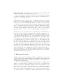
Results on triangulations. In the first set of experiments we computed K-quadtrees
on TIN data for various values of k ≥ 1, denoted QDT-k. The results are shown
in Fig 2 and Fig. 5. Our construction algorithm is significantly faster than qdt1-old (210 minutes vs. 1071 minutes on a TIN with e = 54 · 106 ). As expected,
when k increases, the construction time decreases (Fig 2(a)); the number of cells
in the quadtree decreases (Fig 2(b)) and the overall size of the quadtree decreases
(since fewer cells lead to fewer edge-cell intersections, Fig 2(c)). On the other
hand the average number of edge intersections per cell, l/c, increases (Fig 2(d)).
For example, on a TIN with e = 54 · 106 , QDT-1 is built in 210 minutes,
has c = .6e, l = 2.9e and l/c = 4.8; qdt-100 is built in 57 minutes, and has
c = .004e, l = 1.2e and l/c = 257. Note that l/c represents an average quantity
Quadtree build Time (TIN data, 512 MB)
1.2
Qdt-1-old
QDT-1
QDT-10
QDT-100
QDT-500
Milliseconds per edge
1
QDT-K: e/c (TIN data)
1200
0.8
800
0.6
600
0.4
400
0.2
200
0
107
108
QDT-500
QDT-100
QDT-10
QDT-1
1000
0
107
Number of edges
QDT-K: l/e (TIN data)
4
QDT-K: l/c (TIN data)
QDT-1
QDT-10
QDT-100
QDT-500
3.5
108
Number of Edges
1200
QDT-500
QDT-100
QDT-10
1000
3
800
2.5
2
600
1.5
400
1
200
0.5
0
107
108
Number of Edges
0
107
108
Number of Edges
Fig. 2. Quadtree build times and sizes on TIN data (512MB RAM).
over the entire TIN and the maximum number of edges per cell can be much
higher. In summary, for increasing k, QDT-k is built faster, has smaller overall
size and larger cell size. Table 1 shows the various quadtree sizes and build times
for one of the test TINs. The total size of the quadtree stays consistently small
across all TINs, and appears to grow linearly with the number of edges.
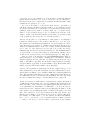
Results on TIGER data. In the second set of experiments we computed Kquadtrees for TIGER data. The results are shown in Fig. 3. Same as for TINs,
the build time gets faster up to k = 100, and then levels. E.g., on EastHalf
(e = 208 · 106 ), it takes 24.7 hours to build QDT-1, 9.0h to build QDT-10, 4.8h
to build QDT-100, and 4.5h to build QDT-500; on AllUSA (e = 428 · 106 ),
qdt-100 can be built in 9.7h. The algorithms run at 70% CPU utilization.
Similar to [7, 6, 8], we found that the bottleneck in quadtree construction is edge
distribution; in our case it accounts for more than 90% of the total running
time, and runs at more than 70% CPU. Even with our new algorithm, building
a qdt-1 is practically infeasible on moderately large data, taking more than 20h.
The average quadtrees sizes are relatively consistent across all datasets, which
is somewhat surprising. qdt-1 has one edge per cell (l/c = 1) on average and an
overall size l = 3e. We also computed the maximum cell size (Fig. 3(c)), which
varies widely from state to state; for example, the largest cell in the EastHalf
bundle intersects 58 edges, while for states like ME and VT, the largest cell intersects 8 edges. For increasing values of k, QDT-k has a larger average cell, but
Build time (TIGER data, 512 MB)
1.4
1.2
Milliseconds per edge
QDT-1 size (TIGER data)
8
QDT-1-old
QDT-1
QDT-10
QDT-100
l/e
l/c
e/c
7
6
1
5
0.8
4
0.6
3
0.4
2
0.2
1
0
105
106
107
Number of edges
108
109
0
105
106
QDT-1: cell size (TIGER data)
50
107
Number of Edges
108
109
QDT-K: l/e (TIGER data)
4
QDT-1: maxcell
QDT-1: l/c
QDT-1
QDT-10
QDT-100
QDT-500
3.5
40
3
30
2.5
20
1.5
2
1
10
0.5
0
105
106
107
number of Edges
108
109
0
105
106
107
Number of Edges
108
109
Fig. 3. Quadtree build times and sizes on TIGER data (512MB RAM).
has fewer cells and an overall smaller size. Empirically, for k = 10, 100, 500, 1000,
QDT-k has l = 1.5e, 1.1e, 1.04e and 1.03e, respectively. Table 2 shows the
quadtree sizes and build times for the EastHalf bundle (e = 208.3 · 106 ).
Segment intersection using quadtrees. To test the efficiency of segment intersection using quadtrees, we ran a set of experiments using a TIN (e = 53.9 · 106 )
stored as QDT-1, and the TIGER datasets stored as QDT-k, for various values
of k. To force all datasets to cover the same area, we scaled them to the unit
square; the resulting intersections are artificial, and we only use them for run
time analysis.
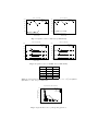
Overall, computing the intersecting segments is fast and scalable. From Table 3 we see that computing the overlay of 262 million edges can be done in under
1.8 hours if the quadtrees are given. Fig. 7 shows the times for k = 1, 10, 100, 500
and 1000. First, we note the big variations in time among the smaller TIGER
sets. We suspect this is because the maximum cell size varies a lot (Fig. 3(c)),
and overlay is sensitive to cell size (for each pair of cells that overlap, all edges
in one are checked against all edges in the other). For the larger TIGER sets, we
see two competing effects in the running time. On one hand, as k increases, the
size of a cell increases, and the time to compute the intersections between two
cells increases. On the other hand, the overall number of cells and edge-cell intersections decrease, resulting in fewer cell-to-cell comparisons. The two effects,
combined, cause the total time to first decrease as k increases from 1 to 100, and
again increase for k = 500. The optimal K-quadtree for segment intersection
against QDT-1 is not the one with k = 1, as one might have expected, but
seems to be one with k ∈ [100, 500].
5
Conclusions
We proposed a simple, i/o-efficient algorithm for the construction of a quadtree
of a set of edges in the plane. For a user defined parameter k ≥ 1, our quadtree
has O(n/k) cells with O(k) vertices each, and can be built in O(sort(n+l)) i/o’s,
where l = O(n2 /k) is the total number of edge-cell intersections. The K-quadtree
can trade off the size of a cell with the number of cells, overall size and construction time, and its i/o-efficient construction is simple and scalable. Our experiments confirm that K-quadtrees are viable for two classes of data used frequently
in practice, TIN and TIGER. In our experiments we use test datasets of up to
427 million edges, two orders of magnitude larger than in related work [7, 6, 8].
References
1. P. K. Agarwal, L. Arge, and A. Danner. From point cloud to grid DEM: a scalable
approach. In Proc. 12th Symp. Spatial Data Handling (SDH 2006), pages 771–788.
2. A. Aggarwal and J. S. Vitter. The input/output complexity of sorting and related
problems. Commun. ACM, 31:1116–1127, 1988.
3. L. Arge, R. D. Barve, D. Hutchinson, O. Procopiuc, L. Toma, J. Vahrenhold, D. E.
Vengroff, and R. Wickremesinghe. TPIE user manual, 2005.
4. M. de Berg, H. Haverkort, S. Thite, and L. Toma. Star-quadtrees and guardquadtrees: I/O-efficient indexes for fat triangulations and low-density planar subdivisions. Computational Geometry, 43(5):493–513, 2010.
5. I. Gargantini. An effective way to represent quadtrees. Commun. ACM,
25(12):905–910, 1982.
6. G. Hjaltason and H. Samet. Improved bulk-loading algorithms for quadtrees. In
Proc. ACM International Symposium on Advances in GIS, pages 110–115, 1999.
7. G. Hjaltason, H. Samet, and Y. Sussmann. Speeding up bulk-loading of quadtrees.
In Proc. ACM International Symposium on Advances in GIS, 1997.
8. G. R. Hjaltason and H. Samet. Speeding up construction of PMR quadtree-based
spatial indexes. VLDB Journal, 11:190–137, 2002.
9. E. Hoel and H. Samet. A qualitative comparison study of data structurers for large
segment databases. In Proc. SIGMOD, pages 205–213, 1992.
10. R. Nelson and H. Samet. A population analysis for hierarchical data structures.
In Proc. SIGMOD, pages 270–277, 1987.
11. H. Samet. Spatial Data Structures: Quadtrees, Octrees, and Other Hierarchical
Methods. Addison-Wesley, Reading, MA, 1989.
12. H. Samet. Foundations of Multidimensional and Metric Data Structures. MorganKaufmann, 2006.
13. H. Samet, C. Shaffer, and R. Webber. The segment quadtree: a linear quadtreebased representation for linear features. Data Structures for Raster Graphics, pages
91–123, 1986.
14. H. Samet and R. Webber. Storing a collection of polygons using quadtrees. ACM
Transactions on Graphics, 4(3):182–222, 1985.
15. L. Toma. External Memory Graph Algorithms and Applications to Geographic
Information Systems. PhD thesis, Duke University, 2003.
6
Appendix
Dataset
Kaweah
Puerto Rico
Cumberlands
Sierra
Central App.
Hawaii
Haldem
Lower NE
e Max inc. Min 6
1.2 · 106
31 .0704
4.1 · 106
291 .0010
5.1 · 106
44 .0016
7.9 · 106
75 .0137
10.1 · 106
62 .0013
19.7 · 106
356 .0007
37.1 · 106
78 .0097
53.9 · 106
168 .0021
Dataset
New England
East Coast
Eastern Half
All USA
e
25.8 · 106
113.0 · 106
208.3 · 106
427.7 · 106
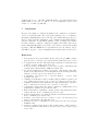
Fig. 4. (a) TIN datasets and their characteristics: the number of edges e, the maximum
degree of a vertex, and the minimum angle (in degrees). (b) TIGER bundles sizes.
c
l
6
6
l/c build (minutes)
QDT-1-old 32.5 · 10 158.8 · 10
4.8
1071
QDT-1
32.5 · 106 158.8 · 106
4.8
210
qdt-10
3.2 · 106 85.9 · 106 26.7
76
qdt-100
0.24 · 106 62.8 · 106 257.4
57
qdt-500
0.06 · 106 58.4 · 106 957.4
53
qdt-1000 0.02 · 106 56.5 · 106 2456.5
54
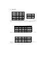
Table 1. Quadtree size and build times on a test TIN dataset (LowerNE, e = 53.9 · 106 )
c
l
6
6
l/c build (minutes)
qdt-1
472.5 · 10 589.7 · 10
1.3
1,482
qdt-10
36.8 · 106 284.4 · 106 7.7
539
qdt-100
3.2 · 106 228.4 · 106 71.4
287
qdt-500
0.6 · 106 216.8 · 106 361.3
273
qdt-1000 0.3 · 106 214.2 · 106 714.0
280
Table 2. Quadtree size and build times on a test TIGER dataset (EastHalf, e =
208 · 106 ).
QDT-K: e/c (TIN data)
1200
QDT-K: l/c (TIN data)
1200
QDT-500
QDT-100
QDT-10
QDT-1
1000
800
800
600
600
400
400
200
200
0
107
QDT-500
QDT-100
QDT-10
1000
0
108
107
Number of Edges
108
Number of Edges
Fig. 5. K-quadtrees sizes on TIN data (512MB RAM).
QDT-K: e/c (TIGER data)
1200
QDT-K: l/c (TIGER data)
1200
QDT-1000
QDT-500
QDT-100
QDT-10
1000
800
800
600
600
400
400
200
200
0
105
106
107
Number of Edges
108
QDT-1000
QDT-500
QDT-100
QDT-10
1000
109
0
105
106
107
Number of Edges
108
109
Fig. 6. K-quadtrees sizes on TIGER data (512MB RAM).
l1 + l2 time (hr)
qdt-1
748.5 · 106
4.5
qdt-10 443.2 · 106
2.3
qdt-100 387.2 · 106
1.8
qdt-500 375.6 · 106
2.7
qdt-1000 373.1 · 106
4.0
Table 3. Segment intersection between qdt-1 (LowerNE, e = 53.6 · 106 ) and QDT-k
(EastHalf, e = 208 · 106 ), 512 MB RAM.
Segment intersection (QDT-1 with QDT-K)
QDT-1000
QDT-500
QDT-1
QDT-10
QDT-100
Microseconds per edge
140
120
100
80
60
40
20
0
108
109
Number of edges
Fig. 7. Segment intersection (overlay) using quadtrees.