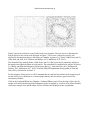
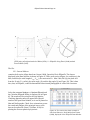
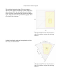
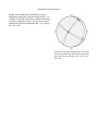
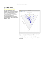
1
EllipseFit 3
User Manual
Version 3.2.0
January 28, 2015
EllipseFit Software
Copyright © Frederick W. Vollmer
1997-2015
Table of Contents
License and Citation
1.
Introduction
1.1 Installation
1.2 Example Data Files
2.
Overview of Strain Analysis
3.
Strain from Points
3.1 Fry Analysis
3.2 Normalized Fry Analysis
3.3 Nearest Neighbor Analysis
3.4 Mean Log Likelihood Function (MLLF)
4.
Strain from Lines
4.1 Analytical Wellman Analysis
4.2 Line Stretch Analysis
5.
Strain from Ellipses and Polygons
5.1 Polygon Moment-Equivalent Ellipses
5.2 Digitizing Ellipses
6.
Ellipse Data Graphs
7.1 Elliott Polar Graph
7.2 Rf ϕ
7.3 Hyperboloidal Projections
7.
Mean Ellipse Calculations
5.1 Shape Matrix Eigenvectors
5.2 Mean Radial Length (MRL)
5.3 Hyperbolic Vector Mean
5.4 Bootstrap Error Analysis
5.5 Simple Means and Centroids
8.
Ellipsoid Calculation
8.1
8.2
8.3
9.
Global Coordinates
Shan Ellipsoid Calculation
Error Analysis
Ellipsoid Data Graphs
9.1 Flinn Graph
9.2 Nadai Graph
10. Data Transformation
11. Data Synthesis
12. Image Analysis
12.1 Filtering
12.2 Edge Detection
Acknowledgements
References
History
License and Citation
License
EllipseFit 3 software and accompanying documentation are Copyright © Frederick W. Vollmer. They
come with no warrantees or guarantees of any kind. The software is free and may be downloaded and
used without cost, however the author retains all rights to the source, binary code and accompanying
files. It may not be redistributed or posted online. It is requested that acknowledgment and citation be
given for any usage that leads to publication.
This software and any related documentation are provided "as is" without warranty of any kind, either
express or implied, including, without limitation, the implied warranties or merchantability, fitness for
a particular purpose, or non-infringement. The entire risk arising out of use or performance of the
software remains with you.
Citation
EllipseFit is the result of many hours of work over several decades. Algorithms used in the program
come from numerous sources, however many have been developed by the author, some of which have
not yet been published and are the subject of papers in preparations. I have released the program
publicly with the hope that the structure and tectonics community will find it useful, and ask
forgiveness for the limited documentation, as well as respect for publication priority.
In return for free use, I request that any significant use of the software in analyzing data or preparing
diagrams be cited and acknowledged in publications, presentations, or other works. An
acknowledgement could be, “I thank Frederick W. Vollmer for the use of his EllipseFit 3 software.”
Appropriate references include (see References):
Vollmer (2010) discusses ellipse and ellipse fitting techniques, including Shan's method, and their
implementation in EllipseFit.
Vollmer (2011a) discusses methods for contouring finite strain on the unit hyperboloid and the use of
hyperboloidal stereographic, equal-area and other projections for strain analysis.
Vollmer ( 2011b) discusses best-fit strain from multiple angles of shear and an analytical solution to the Wellman
diagram.
A suitable references to the software and this documentation, are:
Vollmer, F.W., 2015. EllipseFit 3.2.0. http://www.frederickvollmer.com/ellipsefit/.
Vollmer, F.W., 2015. EllipseFit 3.2.0 User Manual. http://www.frederickvollmer.com/ellipsefit/.
Registration
Please consider registering the software, registration is free and helps me determine the software usage
and justify the time spent in it's upkeep. To register, simply send an email to me at
[email protected] with your user name, affiliation, and usage. I will send you one email in reply
with my thanks, and will not place you on a mailing list. For example, send me an email with
something like:
User:
Affiliation:
Usage:
Frederick Vollmer
SUNY New Paltz, Geology Department
Undergraduate structural geology course and research
I am happy to take emails with questions and suggestions, either at the university (SUNY New Paltz) or
at the gmail address used on my website. However I am not reliable about checking email, so please
forgive me if I am slow in answering, I will try to respond in as timely a fashion as possible.
EllipseFit User Manual Page 1
1.
Introduction
EllipseFit is an integrated program for geological finite strain analysis. It is used for determining two
and three-dimensional strain from oriented photographs, and is designed for field and laboratory based
structural geology studies. The graphical interface and multi-platform deployment also make it ideal for
introductory or advanced structural geology laboratories. I use the software to teach structural geology
at SUNY New Paltz, where hundreds of students have used it in laboratory and field studies. EllipseFit
is currently implemented for Windows 32, Macintosh 10.5+, and Linux (Ubuntu) 64 bit platforms.
EllipseFit is suitable for determining two and three dimensional strain using various objects including
center points (Fry analysis), lines, ellipses, and polygons. Polygons include ooids, pebbles, fossils, or
particles of any initial shape. The analysis of strain from polygons is widely applicable to many rocks
in thin section, hand sample, or suitable outcrops. EllipseFit allows digitizing polygons directly, or
indirectly by using a flood fill method. EllipseFit converts them to moment equivalent ellipses, and the
mean ellipse is equivalent to the strain (Mulchrone and Choudhury, 2004). Given three or more
oriented sections EllipseFit can calculate the three dimensional strain using the method of Shan (2008).
This User Manual was initially prepared for the strain workshop at the 2014 Structural Geology and
Tectonics Forum, at the Colorado School of Mines with Paul Karabinos and Matty Mookerjee, and is
not, however, complete. EllipseFit 3 has numerous improvements over version 2, but has had more
limited testing. Additional releases are planned in the near future. Version 2 is stable and has been
widely used, including for a strain workshop at the 2012 Structural Geology and Tectonics Forum at
Williams College. No updates are planned for EllipseFit 2.
I am a professor of structural geology, and have taught for over 30 years at SUNY New Paltz. I had the
luck to be introduced to analytical structural geology as a student, and am particularly grateful to my
mentors Rob Twiss at UC Davis, Win Means at SUNY Albany, and Peter Hudleston at U Minnesota
whose clear thinking inspired me. I was introduced to programming as a grade school student, when
my dear mother forced me to take a summer school course. I subsequently joined the Computer Club,
as the third member, and spent countless hours on the terminal connected remotely to a mainframe.
Writing code is still an obsession.
The final version of EllipseFit 1 was completed in the 1989 in C++ for Macintosh, in part based on
code from a Fortran program written (on punch cards) for Win Means. Version 2 was written in cross
platform RealBasic, however issues with licensing, cost, performance, and the closed source led me to
abandon that language. Version 3 is fully rewritten, with tens of thousands of lines of code, in Free
Pascal, a professional open source compiler that runs on over 40 operating systems. This allows
improved code with better speed and extensibility, and the potential to port to other platforms. I
simultaneously develop several programs that use common graphics and matrix libraries that I have
written.
1.1 Installation
On Macintosh OS X, double click the disk image file (.dmg), and drag the EllipseFit application to
your Applications folder, or other desired location.
On Windows, unzip the zip file (.zip) using the Extract All option, and drag the EllipseFit folder to any
desired location. The EllipseFit folder contains the EllipseFit application (EllipseFit.exe), and a
“Resources” folder which is required. Please make sure to entirely extract the EllipseFit folder from the
EllipseFit User Manual Page 2
zip file, this is the most common installation problem.
On Linux unpack the gzip file (.tar.gz), and copy the EllipseFit folder to any desired location. The
EllipseFit folder contains the EllipseFit application (ellipsefit), and a “Resources” folder which is
required. An application icon (ellipsefit.png) is included in the Resources folder if desired for
installation.
There is also a folder of example data and images to show how data is formatted, these are referred to
in this guide. After installing a new version it is recommended that you reset the preferences using the
“Reset Preferences” command in the Help menu. This will clear any options that may have changed
and set them to default values. The preferences are stored in the file EllipseFit3.xml, which is located in
the folder EllipseFit in your operating system's application preferences folder. To deinstall simply
delete the EllipseFit application folder, and optionally delete the preference folder. No other files are
installed on your computer. No administrative permissions are required to install EllipseFit, and it is
possible to keep a copy on a thumb drive to run on any computer.
1.2
Example Data Files
The included example files and images can be used to determine input data formats. These are simple
files that can be generated using a text editor or spreadsheet. EllipseFit 3 will read comma separated
(csv), tab separated (tsv), and Open Document (ods) formats. The header line indicates the type of data
required in each column. The included example files are named to indicate their contents (this is not
required, EllipseFit will examine the headers to determine the available data, and extra columns are
ignored):
E2 - Ramsay and Huber 1983 (small).csv
E2 - Ramsay and Huber 1983 (small).jpg
E2 - Ramsay and Huber 1983 (large).jpg
Example ellipse data and thin section photomicrograph (from Ramsay and Huber, 1983). This data type
can contain (X, Y) coordinates for Fry-type analyses, or complete ellipse data including (X, Y, A, B, R,
Phi) axes data. Note that there are small and large versions, I use the large version, which does not
include a data file, for teaching.
E3 - Hossack 1968.csv
Example ellipsoid data (from Hossack, 1968) with (A, B, C) axes data for Flinn and Nadai graphs.
ES - Owens 1984.csv
Example ellipse section data (fron Owens, 1984 ) for calculating the three-dimensional strain ellipsoid
from three or more faces using Shan's (2008) method. The strikes and dips of each section must be
included.
LA - Ragan 1985 F10.1a.csv
LA - Ragan 1985 F10.1a.png
Example line angular shear data and image (from Ragan, 1985) for analytical Wellman-type analysis
(Vollmer, 2011). Each data point requires the endpoints of two lines that originally had a constant
angle. This is an analytical solution to the classic multiple brachiopod problem illustrated in a number
of structural geology texts.
LS - Ragan 2009 T14.9.csv
Example line stretch data for lines with known initial and final lengths, such as boudins and folds.
EllipseFit does not yet provide digitizing of this type of data. Please contact me if this would be of
EllipseFit User Manual Page 3
interest. Note that the LS data is from fold flattening index example (Ragan, 2009), which is
mathematically related.
MLLF Test 60.csv
Sample of 60 points used to test the maximum mean log likelihood function (MLLF) method of Shan
and Xiao (2011).
EllipseFit User Manual Page 4
2.
Overview of Strain Analysis
I was asked by by sister, an artist, to explain the importance of this geological strain analysis that I
spent so much time on. When attempting to unravel the history of a mountain belt, one starts with an
outcrop or a hand sample. The lithology, textures, and mineralogy give clues to the past sedimentary
environment, the temperature and pressure history, and geochronology gives the dimension of time.
Strain analysis gives yet another dimension, a measure of the deformation enjoyed during that history.
Geological strain analysis and theory is an important aspect of structural geology that is covered in
numerous textbooks (e.g., Means, 1976; Hobbs, Means, and Williams, 1976; Ragan, 1985; Marshak
and Mitra, 1988; Van der Pluijm and Marshak, 2004; Pollard and Fletcher, 2005; Twiss and Moores,
2007; Ragan, 2009; Fossen, 2010). Ragan (2009) and Ramsay and Huber (1983) provide excellent
overviews of techniques for the analysis of strain in deformed rocks.
Strain markers can be grouped into three general categories (Lisle, 2010; Mulchrone, 2013): (1) objects
or groups of objects with known pre-strain geometries; (2) objects whose shape may be approximated
by ellipses or polygons; and (3) collections of objects whose spacial arrangement can be used to
determine strain. Category 1 includes fossils and other objects of known unstrained geometry to which
equations of finite strain can be applied (e.g., Ramsay, 1967; Ramsay and Huber, 1983). These
techniques are very useful for specific locations or samples (e.g., Wellman, 1966; Waldon, 1988), but
are less broadly applicable than the other two. EllipseFit implements an analytical Wellman method
(Vollmer, 2011), and a method where multiple line stretches (as from folds and boudins) are known
(Chapter 4). Category 2 includes samples such as sandstones and conglomerates, as well as collections
of irregular clasts or fossils (Mulchrone and Choudhury, 2004), so these techniques are very broadly
applicable. EllipseFit includes numerous procedures to collect and analyze this type of data (Chapters
5). Category 3 includes Fry (Fry, 1979) and nearest neighbor (Ramsay, 1967) methods, EllipseFit
includes numerous procedures related to these (Chapter 3).
The following chapters discuss techniques of strain analysis that are implemented in EllipseFit in terms
of the type of data collected: points, lines, ellipses, and polygons. Points are the simplest type of data
collected, however, as discussed in Chapter 3, Strain from Points, it can be difficult to objectively
extract strain from point distributions. The analysis of line data depends on the known initial lengths of,
or angles between, lines, and has important applications for some data as discussed in Chapter 4, Strain
from Lines.
Chapter 5, Strain from Ellipses and Polygons, covers ellipse data, which is collected assuming that
particles, such as sand grains, initially approximated a collection of random spheres or ellipsoids. It
turns out, however, that ellipse data is a subcategory of polygon data. An important mathematical proof
(Mulchrone and Choudhury, 2004) shows that all particles, of any shape, that can be assumed to have
been initially randomly oriented, can be used to calculate strain. This allows numerous geological
objects to be used for strain analysis using objective calculations developed for ellipse analysis.
Chapter 6, Ellipse Data Graphs covers graphical techniques for two-dimensional strain plots, including
Rf ϕ graphs and polar Elliott graphs, which are types of hyperboloidal projections. Hyperboloidal
projections are analogous to spherical projections, such as the stereographic and equal-area projections
that are used to create stereonets and Schmidt nets respectively, familiar to students of structural
geology.
Chapter 7, Mean Ellipse Calculation, discusses the calculation of a mean ellipse from a sample of
EllipseFit User Manual Page 5
ellipses. As discussed in Chapter 5, these calculations apply to polygons as well as ellipses, as the use
of polygon moment equivalent it ellipses removes the requirement that particles were initially elliptical.
The techniques mentioned thus far are related to two-dimensional strain analysis. Chapter 8, Ellipsoid
Calculation, covers the more complex steps involved in determining three-dimensional strain ellipsoids
from oriented sections for which the two-dimensional strain ellipse has been determined. Chapter 9,
Ellipsoid Graphs, covers strain graphs used to display this type of data, Flinn and Nadia graphs.
Chapter 10, Data Transformation discuses methods for transforming data sets, including unstraining or
retrodeforming data sets and images to their pre-deformation state. Chapter 11, Data Synthesis, covers
data synthesis for making artificial samples from random populations. Chapter 12, Image Analysis
discusses image analysis techniques, including filtering and edge finding, that can aid in highlighting
particle edges prior to digitizing.
It is essential to be aware of the assumptions involved in strain analysis. Refer to the referenced texts
for a complete discussion. An important consideration is whether the particles, such as fossils or clasts,
record the same deformation as the rock. In general, this means whether there was a viscosity contrast
between the particles and the matrix that encloses them. This is discussed briefly in Chapter 3.
A second problem to consider is whether there was an initial preferred orientation of the particles, this
can be related to an initial sedimentary fabric, or compaction. Unimodal, or orthogonal, sedimentary
fabrics and compaction essentially apply a “deformation” that is indistinguishable from a tectonic
deformation without additional information. Detection of initial fabrics is discussed briefly in Chapter
7. Similarly, volume change is difficult to quantify, and strain is generally calculated with volume
equivalent to an initial unit sphere.
This User Manual is written in a tutorial fashion, in order to become acquainted with the program, it is
a good idea to work through the examples provided. This User Manual is also not yet finished, it is a
work in progress.
3.
Strain from Points
It is common in nature for objects to be distributed randomly, but with some minimum cutoff distance
between them. A random distribution in space follows a Poisson distribution (see, for example, Davis,
1986), essentially a distribution gotten by throwing pingpong balls randomly into an empty room.
However, the centers of the pingpong balls can never touch, giving a cutoff distance of twice the radius
of the balls.
This distribution is called a truncated Poisson distribution (e.g., Shana and Xiao, 2011), or an
anticlustered distibution (e.g., Mulchrone, 2013). Examples of this type of data include the centers of
clasts in many sedimentary rocks such as sandstones and conglomerates. The centers of phenocrysts in
igneous rocks, where nucleation of new crystals is prevented in proximity to existing crystals due to the
chemical gradient, is another example. Note that if the particles have a different viscosity than the
enclosing matrix, even if they are perfectly rigid, it is possible to get an estimate of the strain of the
rock. Thus it is possible to extract different information than by an analysis of the particle shapes.
The basic idea for methods utilizing point distributions (e.g., Ramsay and Huber, 1983) is that the
distance between the initial object centers is the same in all directions, and after a deformation the
particles are closer in some directions and further in others. This new distribution will be elliptical in
two dimensions, or ellipsoidal in three-dimensions.
EllipseFit User Manual Page 6
Two general methods have been proposed for analyzing this type of data, a nearest neighbor approach
(Ramsay, 1967; Ramsay and Huber, 1983), and an all object separation approach (Fry, 1979),
commonly referred to as the Fry method. The latter, initially graphical approach, has many variations,
one of the most common is the normalized Fry method (Erslev, 1988; Erslev and Ge, 1990). It is
important to note that the normalized Fry method requires the particle shape (as an ellipse), and
therefore the distinction between Category 2 and Category 3 data (Chapter 2) becomes blurred, or lost.
If it can be assumed that the strain of the particles reflects the strain of the rock, then it is preferable to
use the Category 2 methods as discussed in Chapter 5.
The nearest neighbor approach (Section 3.3) has been enabled computationally by the availability of
Delaunay triangulation algorithms (e.g., Preparata and Shamos, 1985; Lischinski, 1994). This approach
was initially used in EllipseFit 1 (Vollmer, 1989), and has been developed by Mulchrone (Mulchrone,
2003; Mulchrone, 2013).
A difficult problem in point data analysis is to determine the strain ellipse from the central void. The
enhanced normalized Fry method (Erslev and Ge, 1990) was developed to solve this, but requires the
particle ellipse, and also a subjective parameter, the selection factor (Section 3.2). As discussed above,
this blurs the distinction between Category 2 and 3 data. A number of solutions to this problem using
only point data (Category 3) exist (e.g., Lisle, 2010; Shan and Xiao, 2011; Waldron and Wallace, 2011;
Mulchrone, 2013). Currently EllipseFit implements the algorithm of Shan and Xiao (2011), discussed
in Section 3.4.
3.1
Fry Analysis
A Fry analysis (Fry, 1979) is an important and widely used technique for analyzing this type of data,
and there is an extensive literature on it and its variations (e.g., Hanna and Fry, 1979; Crespi, 1986;
Onasch, 1986; Erslev, 1988; Erslev and Ge, 1990; Dunne, Onasch, and Williams, 1990; McNaught,
1994; McNaught, 2002; Shan and Xiao, 2011; Waldron and Wallace, 2011; Mulchrone, 2013).
A Fry analysis can be simply done with two pieces of tracing paper, by tracing all of the particle centers
on one sheet, then drawing a center point on a second sheet overlain on the first, and then sequentially
moving the center point to each point and trace each point. For n initial points, this generates:
nf = n! / (2 * (n - 2)!)
points, which is a lot of points to draw by hand. To illustrate the use of the method in EllipseFit, start
EllipseFit and open the file (File > Open):
E2 - Ramsay and Huber 1983 (large).jpg
This is a photograph of a deformed ironstone oolith in thin section from Ramsay and Huber (1983) that
is widely used as a test image for strain analysis. For point digitizing make sure the red Point Icon
(second from left) is displayed (Digitize > Center Point), and the green Plus Icon is selected (Digitize >
Add Tool), as in Figures 1 and 2.
EllipseFit User Manual Page 7
Use the zoom tools to enlarge the image,
and click on one particle center. The
Data Window will open and display a
highlighted line of data. Before
continuing, open the Fry graph (Analyze
> Fry Graph). You should have
something similar to Figure 2.
Figure 1. EllipseFit's Image Window used for digitizing, with
photomicrograph of a deformed oolite from Ramsay and Huber
(1983).
Continue digitizing point centers, you should ideally work out from one point digitizing adjacent points
keeping a roughly circular area. The Fry graph will start to develop as you digitize, with each new set
of generated points highlighted (Figure 3).
EllipseFit User Manual Page 8
Figure 2. EllipseFit's Image Window, Data Window and Fry Graph displaying a single data
point.
Use the Hand Tool (Digitize > Hand Tool, or the Hand Icon) to scroll, and the Zoom Tool to zoom
(Digitize > Zoom or the Magnifying Glass Icon). You can also use the Command (Mac) or Control
(Windows and Linux) + and – keys to zoom in and out. Holding down the Shift key allows scrolling
with the cursor. Points can be deleted by using the Find Tool (Digitize > Find Tool or the Binoculars
Icon) to highlight a point, and delete it using the Cut command (Edit > Cut) or red X Icon. A point can
also be deleted by selecting it in the Data Window and deleting it there.
It is important to be objective, and you may wish to digitize all available points, however note that
some particles may not meet the required assumptions. In particular, note that the centers of the
particles in two-dimensions do not generally correspond to their three-dimensional centers, as they lie
on an arbitrary plane cutting through the rock, so the assumption of of a uniform cutoff is weakened.
This is discussed further in Section 3.2, Normalized Fry Analysis.
Additionally, it is desirable to select approximately equal numbers of particles in all directions, so the
point density is not biased by direction. This is one reason to maintain a uniform point density in a
circular area while digitizing, and why having the interactive Fry graph open can assist in particle
selection. This is discussed further in Section 3.2, Mean Log Likelihood Function (MLLF).
EllipseFit User Manual Page 9
Figure 3. Fry graph after digitizing 20 adjacent particle centers. The generated points are
highlighted. On the right, note the presence of the spurious data point (each point is mirrored
about the center) generated by clicking too close to an existing point, i.e. an operator error which
can be deleted.
If you wish to change the size of the
digitized points, click the Gear Icon (or
Preferences) from which you can set
most of the EllipseFit preferences. Note
some selections have multiple pages,
use the left-right arrows (Command < >)
to go through them. You can preview the
effect of preference changes before
setting then with the OK button.
To view the data as a Strain Map select
Analyze > Strain Map. This displays the
data as particle centers, this population
can be strained and unstrained as
described in Chapter 10, Data
Transformation.
Figure 4. The EllipseFit Preferences Dialog where most
preferences are set. Note the left-right arrows used to scroll to
additional pages if present.
EllipseFit User Manual Page 10
Figure 5 is the graph after carefully selecting 60 particle centers, a probable minimum number for
analysis (Shan and Xiao 2011), and after digitizing 252 points, essentially all of them.
Figure 5. Fry graphs after digitizing 60 carefully selected points, and after digitizing 252 points,
essentially all of them. These images are PNG files as saved from EllipseFit.
To zoom in for a better image of the central void, open the Preferences Dialog (Gear Icon), uncheck
Auto-scale, and enter a number smaller than the displayed Data radius (Figure 6).
Figure 6. Set the graph radius to display the central void by unchecking Auto-scale, and entering
a smaller radius.
EllipseFit User Manual Page 11
Figure 7. Close up of the central voids for the two data examples of 60 and 252 points.
Figure 7 shows the zoomed in central voids for the two examples. The next step is to determine the
best-fit ellipse for the central void displayed in Figure 7. This can be a subjective process, and
objectively choosing this ellipse is the subject of a number of papers (e.g, Erslev, 1988; Erslev and Ge,
1990; Shan and Xiao, 2011; Waldron and Wallace, 2011; Mulchrone, K.F., 2013).
The normalized Fry method (Erslev, 1988; Erslev and Ge, 1990) is one that is commonly employed,
but requires the digitized ellipses of each particle. The normalized Fry method is the subject of Section
3.2. Ideally a method should require only the point data (e.g., Shan and Xiao, 2011; Waldron and
Wallace, 2011; Mulchrone, K.F., 2013). Currently EllipseFit implements the algorithm of Shan and
Xiao (2011), discussed in Section 2.3.
For the purposes of this section, it will be assumed that the void has been defined well enough to pick
out the void by eye, which may be a close enough estimate, and also makes a good exercise for
introductory students.
Click on the Centered Ellipse Icon (Digitize > Centered Ellipse), and click at the edge of the void. An
orange circle marks the starting point, subsequent points are marked by a yellow circle. When finished,
click on the orange circle and the ellipse will be calculated and displayed in the Log Window.
EllipseFit User Manual Page 12
Figure 8. Digitizing the central void. The orange point is the start point, the yellow are subsequent
points. Click on the orange point when finished, and the ellipse is calculated. The point size is set
larger than the default size for the illustration.
For this sample, the calculated results are reported by EllipseFit as:
N = 60
Pairs = 1770
Best-Fit Ellipse
Manual
n = 17
R = 1.758
Φ = 25.45°
RMS = 0.0583
A centered ellipse was calculated from the 17 digitized points. The calculation is rotationally invariant,
and the best fit found by minimizing the sum of the squares of the distance of the points from the
ellipse, i.e., the residuals. The minimization is solved from the linear equations using a LU
decomposition.
The RMS value is the root mean square measure of the
variation of the residuals from the ellipse, that is the
square root of the sum of the squares of the residuals of
the data from the fitted ellipse. RMS is a common way
to express goodness of fit of least squares solutions. It
is not a measure of the error in the strain calculation,
and is not technically an error. It is, however, a
measure of how closely the digitized points fit the
ellipse. A small RMS means that the entered points lie
close to an ellipse. It makes a good class exercise for
students to solve and compare their results and RMS.
Figure 9. The Transform Image dialog with
values entered to unstrain the mage.
EllipseFit User Manual Page 13
As a final step in this analysis, select the Edit > Transform Image command and enter the results into
the dialog as in Figure 9. The image will be unstrained to remove the calculated strain as shown in
Figure 10.
EllipseFit User Manual Page 14
Figure 10. The oolith photomicrograph after being unstrained using EllipseFit's Image Transform
command.
EllipseFit User Manual Page 15
Next select the Analyze > Transform Data command
and enter the calculated values as shown in Figure 11.
Press Transform and then Accept.
Figure 11. The Transform Data dialog with
values entered to unstrain the data. Set Mean is
only used with ellipse data. Rectify resolves the
offsets caused by the image transformation.
The data is unstrained using the calculated values, as
shown by the Fry graph in Figure 12. The Rectify
option resolves the offsets caused by the image
transformation, so the data points remain centered over
the particle centers.
Figure 12. Fry graph of the unstrained 60 point
data after using the Transform Data command to
unstrain (retrodeform) the data using the
calculated values.
EllipseFit User Manual Page 16
3.2
Normalized Fry Analysis
As discussed in Section 3.1, the Fry analysis is a two-dimensional solution to a three-dimensional
problem, since initial particles are assumed circular instead of spherical. Even if the particles have a
uniform size, a section through a sample will show them as different size particles. One solution
developed to overcome this is the normalized Fry analysis (Erslev, 1988; Erslev and Ge, 1990
McNaught, 1994; McNaught, 2002).
The distances between particles are normalized to account for the difference in the sizes of the
particles, which can greatly improve the sharpness of the central void. Unfortunately, the ellipse sizes
and orientations are required for this, and in most cases if the ellipse data is available, it should used for
the strain analysis following techniques in Chapter 7, Strain from Polygons. However, as mentioned in
Section 3.1, a Fry analysis can provide different information regarding particle versus matrix strains.
The digitizing of ellipses is discussed in Chapter 5, Strain from Ellipses, so for an example of this
analysis, open the image file:
E2 - Ramsay and Huber 1983 (small).jpg
and the data file:
E2 - Ramsay and Huber 1983 (small)
This is the 252 point data set used in Section 3.1.
The data is overlain on the image, and, if the Binoculars Icon is selected, you can select individual
particles that are highlighted in the Data Window and the Fry Graph. This selection method is
implemented for most of the graphs discussed in subsequent chapters. The Fry graph will look like
Figure 5B.
EllipseFit User Manual Page 17
Figure 13. EllipseFit Image Window with ellipse data overlain. Selecting the Binoculars Icon
(as shown) allows interactive selection of particles that are highlighted in the Data Window, as
well as on data graphs including the Fry Graph.
To zoom in on the central void, open the Preferences
Dialog (Gear Icon), deselect Auto-scale, and enter 50
for the Graph radius as shown in Figure 14.
Figure 14. Settings to display the central void
without normalizing.
EllipseFit User Manual Page 18
The unnormalized graph is displayed in Figure 15.
Figure 15. The Fry graph without normalizing,
using the settings displayed in Figure 14.
To normalize the graph select Normalize, as shown in
Figure 16. Note that the Normalized radius is now used
due to the normalization to a unit circle, the default
value is 1.5 as shown.
Figure 16. Settings to display a normalized Fry
graph. Note that the Normalized radius is now
used due to the normalization to a unit circle.
EllipseFit User Manual Page 19
The resulting normalized graph is shown in Figure 17.
Note the clear sharpening of the central void.
The final question addressed in his section is how to
find the ellipse corresponding to the central void. The
enhanced normalized Fry method (Erslev and Ge,
1990) uses a user specified cutoff radius to exclude
particles beyond the a certain distance from the void
center. This is a subjective value, chosen here with a
default value of 1.05. In the Preferences Dialog check
Normalize, and uncheck Show all points. EllipseFit
calculates the best-fit ellipse through the cloud of
points using the least squares method described in
Section 3.1.
Figure 18. Settings to display an ehanced
normalize graph.
Figure 17. Graph of the normalized data. Note
the better resolution of the central void.
The results from the Log Window are:
N = 252
Pairs = 31626
Normalized
Enhanced
Selection factor = 1.050
Enhanced pairs
= 142
Best-Fit Ellipse
Automatic
n = 142
R = 1.581
Φ = 24.46°
RMS = 0.1383
Figure 19. Fry graph with ellipse fitted to the
enhanced normalized points.
Again, the RMS is a measure of the deviations of the
residuals, and can be used to refine the selection factor.
However, note that smaller number of points will generally have a smaller RMS. For example three
points give RMS = 0, so finding the minimum RMS is not a valid strategy.
EllipseFit User Manual Page 20
Section 3.3
Nearest Neighbor Analysis
[Documentation in preparation]
Section 3.4
Mean Log Likelihood Function (MLLF)
Calculating the strain from a sample of points should ideally require no additional information about
the particle's shapes, and there are a number of methods that have been developed for this purpose (e.g.,
Lisle, 2010; Shan and Xiao, 2011; Waldron and Wallace, 2011; Mulchrone, 2013). EllipseFit
implements the mean log likelihood function (MLLF) method of Shan and Xiao (2011). They examine
the statistics of a truncated Poisson distribution, and define the MLLF as the average sum of the log
probability distribution function (PDF) of each individual point in the deformed state. This is related to
the density distribution around each point.
The PDF in the deformed state is related to the pre-deformation PDF by the shape and orientation of
the central void, giving as parameters a cutoff distance, the ratio R, and the orientation Φ. The function
is complex however, and is solved using a gird search to locate the maximum MLLF. The search is
over the range Φ = 0° to 179° in steps of 1°, and R = 1 to 20 in steps of 0.1. The latter value is the
default that can be changed if desired, a smaller value will speed up the search. Once R and Φ are
determined, the sample is retro-deformed, and a 50 step search is done to locate the cutoff radius.
Shan and Xiao (2011) further suggest an approach to improve the results using a cross validation
technique for detecting spurious points by sequentially removing up to 10 points, the default value in
EllipseFit, and repeating the search. These algorithms were implemented by Y. Shan in a Fortran
program which he provided, EllipseFit has been carefully tested to insure that identical results are
obtained.
The result are the best estimates values of R, Φ. initial cutoff distance, and a set of neighborhood
points. This method has advantages in that it is a robust numerical solution, and one that uses all of the
points to define the central void. In comparison, the enhanced normalized Fry method that only
examines the points close to the void.
A disadvantage of the method is the computing time required to calculate the solution. In particular the
cross-validation can take several hours. Shan and Xiao (2011) also note, wryly, that it is a pity that the
treatment does not require the Fry plot, which will disappoint structural geologists who prefer manual
manipulation and visual appreciation. To assist, I have tried to make the output plot as visually pleasing
as possible.
To run a test sample open the file MLLF Test 60.csv. This data is the 60 point oolth sample used in
section 3.1, and was carefully selected to avoid spurious points, and to avoid a directional bias.
EllipseFit User Manual Page 21
Select the command Analyze > Calculate Ellipse . Note
that the only available options are the MLLF options,
the other options all require ellipse data. Select Mean
log likelihood, leave Cross validate off as in Figure 20,
and press OK.
A progress dialog will appear as in Figure 21, the
display shows the search iteration passes in degrees,
and is done at 180. The process should complete in less
than a minute, and the results displayed in the Log
Window, and on the Fry Graph (Figure 22).
Figure 20. The Calculate Ellipse Dialog
showing the MLLF options available for a set of
point-only data.
Figure 21. Progress dialog for the MLLF grid
search without cross validation.
The results reported in the log file are:
N = 60
MLLF Calculations
–---------------Pass
Mean LL
R
Phi
0
-0.31829
1.90 25.00
MLLF Results
–----------Point statistics:
Number
Calculated density
Real density
Results:
Mean log-likelihood
R, strain ratio
Phi, angle of max strain axis
Cutoff radius
Cutoff
86.98953
=
=
=
60
0.00004
0.00000
=
=
=
=
-0.31829
1.90000
25.00000
86.98953
Stat
0.67361
Density
0.84687
EllipseFit User Manual Page 22
EllipseFit User Manual Page 23
Figure 22. Fry graph with results of the mean log likelihood function (MLLF) maximization
search. The ellipse is the result of the MLLF grid search. The green markers highlight the Fry
neighbor points.
The Fry graph of the mean log likelihood function (MLLF) maximization search results is shown in
Figure 22. The ellipse is the result of the MLLF grid search. The green markers highlight the Fry
neighbor points, those that maximize the MLLF. Note the ellipse is the result of the intensive grid
search, and is not simply a linear least squares fit as used in Sections 3.1 and 3.2.
EllipseFit User Manual Page 24
To test the cross validation procedure, go back and
check the Cross validation option in the Preferences
Dialog. The progress dialog now is displayed as in
Figure 23. There are now three iteration passes
displayed, the first is 0 to 10, where 0 is the first
calculation as done above. Passes 1 to 10 are the coss
validation iterations, 1 to 60 are the data points, and 1
to 180 are the Φ grid search in degrees. The R grid
search values (0.1 to 20.0 by default), and the 1 to 50
distance search loops are not displayed.
Figure 23. Progress dialog for the MLLF grid
search with cross validation.
The MLLF search is computationally intensive,
especially for cross validation (during some test runs I
set my laptop on marble coasters to keep it from
overheating). After about 6 hours (on a 3.06 GHz Intel
Core 2 Duo iMac) the process completes, and the
dialog displays OK. You can cancel the run at any time,
and the results of the completed passes will be
displayed.
Mean Ellipse Calculations
MLLF Test 60.tsv
2014-05-31 16:30:46
==============================
N = 60
MLLF Calculations
----------------Pass
Mean LL
R
Phi
0
-0.31829
1.90 25.00
1
-0.31610
1.90 25.00
2
-0.31603
1.90 25.00
3
-0.31882
1.90 25.00
4
-0.31651
1.90 25.00
5
-0.31536
1.90 25.00
6
-0.32428
1.80 23.00
7
-0.31554
1.90 25.00
8
-0.31327
1.90 25.00
9
-0.31454
1.80 23.00
10
-0.31451
1.90 25.00
MLLF Results
-----------Point statistics:
Number
Calculated density
Real density
Results:
Cutoff
86.98953
86.98953
86.98953
86.98953
86.98953
86.98953
87.24708
86.98953
86.98953
87.24708
86.98953
=
=
=
52
0.00004
0.00004
Figure 24. Progress dialog for the MLLF grid
search with cross validation when complete.
Stat
0.67361
0.68773
0.69522
0.67496
0.68968
0.70494
0.68393
0.69945
0.71578
0.69591
0.69099
Density
0.84687
0.86122
0.87607
0.89144
0.90736
0.92386
0.93542
0.95872
0.97716
0.99044
1.01624
EllipseFit User Manual Page 25
Mean log-likelihood
=
R, strain ratio
=
Phi, angle of max strain axis =
Cutoff radius
=
Finished: 2014-05-31 22:49:58
-0.31327
1.90000
25.00000
86.98953
EllipseFit User Manual Page 26
The results of pass 0 are identical to the previous result, however the cross-validation procedure located
a slightly better solution, in pass 8 the mean log likelihood is -0.31327, instead of -0.31829. The
resulting Fry graph with 8 less neighbor points is shown in Figure 25.
Figure 25. Fry graph of the results using the cross-validation option for mean log likelihood
maximization.
EllipseFit User Manual Page 27
4.
Strain from Lines
[Documentation in preparation]
4.1
Analytical Wellman Analysis
The Wellman method can be applied to objects in which two lines can be identified that have constant
initial angles, such as brachiopod hinge and medial lines which are initially perpendicular (Wellman,
1962; Ramsay, 1967). For brachiopods not parallel to a principal strain, this angle will be distorted by
shear strain.
Wellman's graphical technique is illustrated in many structural
geology laboratory manuals (e.g., Ragan, 2009). An analytical
solution to the problem was given by Vollmer (2011), which is
implemented in implemented in EllipseFit. To try the method, open
the file
LA - Ragan 1985 F10_1a.png
as an image. This is from Ragan (1985), and is used in many
structural geology classes as an exercise. To begin click on the
digitizing icon at, the second from the left, until the LinePair Icon is
displayed, or from the menu choose Digitize Line Pair. Click on the
endpoints of each of the two lines in turn. When done the lines
appear in red, and the yellow cursor appears at the intersection.
Mistakes can be corrected by using the red X Cut Icon, or by deleting
the line pair in the Data Window.
Figure 26. The Image Window
after opening the example data
for the analytical Wellman
method from Ragan (1985). The
hinge and medial lines are
assumed initially perpendicular.
One line pair has been
digitized.Note the Line Pair Icon
is visible.
EllipseFit User Manual Page 28
After digitizing one line pair, open the Wellman Graph
using the menu command Analyze > Wellman Graph.
The graph shows the parallelogram corresponding to
the brachiopod (Figure 27). The parallelogram sides
parallel the line pair. Note the two additional points
used for the construction.
Figure 27: The analytical Wellman graph
diplayed in a graph window after digitizing one
line pair as in Figure 26. Note the Binoculars
Icon is selected and that the parrallelogram and
corresponding brachiopod are selected with the
yellow cursor.
Continue digitizing the remaining line pairs. Figure 28
shows the graph after three line pairs. The yellow cross
cursor highlights the corresponding data point
intersection and parallelogram, and the data is selected
in the Data Window. If the Binoculars Icon is pressed,
as in Figure 28, you can search on the graph to locate
the corresponding data. As in digitizing points, this
allows the identification of outliers or spurious data.
Figure 28: The analytical Wellman graph after
three line pairs have been digitized.
EllipseFit User Manual Page 29
EllipseFit User Manual Page 30
Figure 29: The final analytical Wellman graph after all 8 line pairs from the brachiopods in Figure
27 have been digitized.
Figure 29 shows the final analytical Wellman graph after all 8 line pairs have been digitized. Examine
the Log Window (Window > Log) and note that at each step EllipseFit calculated the best-fit ellipse.
Analytical Wellman Ellipse Results
Wellman Data.tsv
EllipseFit User Manual Page 31
2014-06-01 21:39:47
==============================
N
= 8
Point pairs = 9 (symmetric)
R
= 1.773
Φ
= 96.10°
n
= 9
RMS
= 0.025
The calculation is the same as described in Sections 3.1 and 3.2, minimizing the sum of the squares of
the residuals the points from the ellipse using a LU decomposition. Similarly, the RMS value is the
root mean square measure of the variation of the residuals from the ellipse, that is the square root of the
sum of the squares of the residuals of the data from the fitted ellipse. It is a measure of goodness of fit
of the ellipse, but is not technically an error. The RMS will be zero for two line pairs. The calculation
includes the constriction line, so the ellipse has 9 point pairs including the 8 data points.
In theory, objects like graptolites that have a constant, non-perpendicular, angle between stipe and
thecae, can be treated in the same fashion (Ramsay, 1967). Dirringer and Vollmer (2013) compared the
automated Wellman method and the mean polygon moment ellipse method (Section 5.1) using a sample
of slate with deformed Ordovician graptolites. The sample was oriented with the slaty cleavage as the
X axis. The center lines and lower thecae lines were digitized in 120 locations for the Wellman test,
only one species had clearly defined thecae lines. The outlines of 31 whole graptolites and 38 partial
graptolites were digitized for the polygon method test.
The mean polygon moment ellipse was R = 2.079 ± 0.122, Φ = 177.48° ± 4.57°, parallel to the slaty
cleavage. The polygon method does not require assumptions about initial shapes, only that they are
initially random. Interpreting the data for the analytical Wellman method was problematic, as it many
outliers around a central ellipse. Removal of 77 outliers, believed to be due to initial variations in
thecae angle, was required before the ellipse could be clearly resolved. While most outliers could be
clearly identified, the process was subjective, and single outliers significantly effected the result. The
result for 43 data points was R = 2.761, Φ = 0.50°, RMS = 0.294, parallel to cleavage.
They concluded that the necessary assumptions about initial geometry for the analytical Wellman
method were not met, and the polygon method, with no such required assumptions about initial
geometry, was preferred.
EllipseFit User Manual Page 32
Figure 30: Sample of deformed graptoliferous slate used by Dirringer and Vollmer
(2013) for comparison of the automated Wellman and mean polygon moment
ellipse methods.
Figure 31: The graptoliferous slate sample of
Figure 24 after retrodeforming to remove the
strain calculated by the mean polygon
moment ellipse method, R = 2.079, Φ =
177.48°
EllipseFit User Manual Page 33
4.2
Line Stretch Analysis
[Documentation in preparation]
5.
Strain from Ellipses and Polygons
[Documentation in preparation]
5.1
Digitizing Ellipses
[Documentation in preparation]
5.2
Moment-Equivalent Polygons
[Documentation in preparation]
EllipseFit User Manual Page 34
6.
Ellipse Data Graphs
[Documentation in preparation]
6.1
Elliott Polar Graph
[Documentation in preparation]
The polar Elliott graph (Elliott, 1970) is a polar plot of
the natural log R and 2ϕ. This is a natural parameter
space for strain, and the graph is a simple
hyperboloidal projection that gives an undistorted
representation (Yamaji, 2008; Vollmer, 2011), It is
therefore generally preferred over the R f ϕ graph of the
next section.
Most of the graphs in EllipseFit are interactive. When
the Binoculars Icon is selected, points can be selected
and the selection will automatically update on other
graphs and in the Data Window.
Figure 32. Polar Elliot graph with digitized data
from the oolith photomicrograph in Figure 1.
One outlier is selected.
EllipseFit User Manual Page 35
EllipseFit User Manual Page 36
EllipseFit User Manual Page 37
To illustrate, Figure 33 shows a Fry graph with the points generated by the outlier selected in Figure 32.
Figure 33. Fry graph with data generated from
the oolith photomicrograph in Figure 1. The
selected points are those generated by the outlier
selected in the polar graph of Figure 32
This outlier falls well inside the central void, and probably does not meet the assumptions necessary for
a Fry analysis, i.e., a truncated Poisson distribution.
6.2
Rf ϕ
[Documentation in preparation]
The Rf ϕ graph (Dunnet, 1969) is probably more widely
recognized and used than the polar Elliott graph (e.g.,
Lisle, 1985), however it distorts the strain space,
especially at low strains, and a polar graph is generally
preferred (Vollmer, 2011).
Figure 34. Rf ϕ graph with digitized data from
the oolith photomicrograph in Figure 1. One
outlier is selected, the same as in Figures 32 and
33, all of which are automatically updated
interactively.
EllipseFit User Manual Page 38
6.3
Hyperboloidal Projections
[Documentation in preparation]
Figure 35: The unit hyperboloid, H2, showing cartesian axes, x0, x1, x2, and point C = (1, 0, 0), which
corresponds to the circle R = 1. The plane x1x2 is the projection plane for azimuthal projections, the polar strain
graph. Points on H2 are x = (x0, x1, x2)T, with origin C. If strain is represented by (ρ, ψ) = (log R, 2ϕ), then an
ellipse is x = (cosh ρ, sinh ρ cos ψ, sinh ρ sin ψ)T
EllipseFit User Manual Page 39
Figure 36: The unit hyperboloid with superimposed cylinder with axis x0. The cylinder is the projection surface
for cylindrical projections, as the Rf ϕ graph.
EllipseFit User Manual Page 40
Figure 37. Synthetic data of 300 ellipses strained to values of
R = 2 and R = 4 displayed on hyperboloidal azimuthal
projections: (a) equidistant, (b) stereographic, (c) equal-area,
(d) orthographic, and (e) gnomic.The best-fit ellipse is
plotted as a white circle, the centroid of the projected data is
plotted as a gray circle.
EllipseFit User Manual Page 41
7.
Mean Ellipse Calculation
[Documentation in preparation]
Data Set
Oolith
n = 252
Imposed (R, ϕ)
1, 0
0.614, 25.74
Synth 1
n = 300
1, 0
2, 0
4, 0
Synth 2
n = 1000
1, 0
2, 0
4, 0
Eigenvector
Mean Radial Hyperbolic
1.628, 25.74
1.628, 25.74 1.628, 25.74
± 0.018, 0.73
± 0.018, 0.62
± 0.013
1.000, 113.32 1.000, 113.32 1.000, 113.32
± 0.007, 55.27 ± 0.011, 633.74
± 0.013
1.031, 40.20
1.031, 40.20 1.031, 40.20
± 0.021, 33.24 ± 0.025, 22.81
± 0.030
2.012, 1.16
2.012, 1.16
2.012, 1.16
± 0.048, 1.16
± 0.050, 0.92
± 0.032
4.023, 0.46
4.023, 0.46
4.023, 0.46
± 0.101, 0.53
± 0.099, 0.37
± 0.031
1.016, 146.03 1.016, 146.03 1.016, 146.03
± 0.012, 35.35 ± 0.014, 24.51
± 0.016
2.012, 179.46 2.012, 179.46 2.012, 179.46
± 0.026, 0.71
± 0.27, 0.51
± 0.016
4.024, 179.78 4.024, 179.78 4.024, 179.78
± 0.052, 0.30
± 0.053, 0.21
± 0.017
Table 1: Comparative results for ellipse-fitting techniques implemented in EllipseFit.
Eigenvector = Shape matrix eigenvectors (Shimamoto and Ikeda, 1976). Radial = Mean
radial length (Mulchrone, et al, 2003; Mulchrone, 2005). Hyperboloidal = Hyperboloidal
vector mean (Yamaji, 2008). From Vollmer (2010).
Shape-matrix eigenvector (Shimamoto and Ikeda, 1976), mean radial length (Mulchrone et al., 2003),
and hyberbolic vector mean (Yamaji, 2008) ellipse-fitting methods give precisely identical results.
7.1
Shape Matrix Eigenvectors
[Documentation in preparation]
7.2
Mean Radial Length (MRL)
[Documentation in preparation]
7.3
Hyperbolic Vector Mean
[Documentation in preparation]
EllipseFit User Manual Page 42
7.4
Bootstrap Error Analysis
[Documentation in preparation]
Figure 38: The best-fit strain ellipse is simply
the hyperboloidal vector mean, which gives
identical values to other methods (Yamaji 2008;
Vollmer, 2010). Error analysis is shown by an
equidistant azimuthal graph of bootstrap results
of 1000 resamples from oolite data. The mean
vector of the bootstrap mean vectors is rotated to
C. The dispersion of the points is a measure of
the error in the best-fit ellipse.
7.5
Simple Means and Centroids
[Documentation in preparation]
EllipseFit User Manual Page 43
8.
Ellipsoid Calculation
For regional strain studies it is generally necessary to determine the three-dimensional strain ellipsoid,
with three stretches and their orientations, normally expressed as trends and plunges. This can be
simplified if assumptions can be made about the relationship between foliations and strain, for example
slaty cleavage is commonly assumed perpendicular to the minimum stretch. However, in the general
case it is necessary to determine the two-dimensional strain on a number of different planes through a
sample (or outcrop where it can be considered homogeneous), and combine them to determine the
strain ellipsoid in three dimensions. This is a difficult mathematical problem, and numerous solutions
have been proposed (e.g., Shimamoto and Ikeda 1976; Owens, 1984; Robin, 2002; Shan, 2008;
Mookerjee and Nickleach, 2011). EllipseFit implements the method of Shan (2008) as discussed in
Section 8.2.
8.1 Global Coordinates and Sample Collection
The two-dimensional strain ellipses considered thus far have been referred to X, Y coordinates, where
X is to the right, and Y is down the image. These coordinate axes are indicated by the blue lines on the
top and left of the Image Window. The angle ϕ is the positive angle (clockwise) from X. This
coordinate system was chosen to simplify the relationship to the global coordinates referred to here as
X', Y', Z', and to simplify the calculation of the three-dimensional strain ellipsoid. The global
coordinates are equivalent to North, East, Down (NED).
In Figure 39 the gray plane is a section plane that
corresponds to an image analyzed for two-dimensional
strain as discussed in earlier chapters. The X axis is
parallel to the strike of the plane, using the standard
right hand rule (e.g., Pollard and Fletcher, 2005), as
shown in Figure 37. The strike is given by θ, the
clockwise angle from North, the standard azimuth in
degrees. The dip of the plane is the angle δ. The
calculated strain ellipse is given by R = A/B =
LMax/LMin, and ϕ, the angle from X, which is its pitch in
global coordinates. This is referred to here as a section
ellipse.
In order to calculate the strain ellipsoid from the
section ellipses, each section ellipse must undergo a
coordinate transformation from local X, Y coordinates
to global X', Y', Z' coordinates. This is done
automatically by EllipseFit, but the user must take
great care to properly prepare samples. Time taken at
this stage will save much aggravation later on.
A sample collected in the field must be carefully
oriented, recording its strike and dip (other conventions
are fine, but the strike is the X coordinate axis so is
used here). A suitable marking is a strike arrow and a
dip tick (Figure 39), if possible on a surface that is not
Figure 39: Coordinate system for section
ellipses. The global coordinates are X' = North,
Y' = East, and Z' = Down (NED). The plane
with the section ellipse has a strike, θ (using the
right hand rule), and dip, δ. The section ellipse
has a pitch, ϕ, and R = A/B, where A and B are
the maximum and minimum axes. A suggested
strike arrow and dip tick marking is shown.
EllipseFit User Manual Page 44
overhanging.
A minimum of three sections must be made through the sample, although more is preferred. Shan's
method (Section 8.2) relaxes this requirement if lineation data is used as well, but Vollmer (2010)
showed that the error range in natural samples can be large, so a minimum of three sections is
recommended. If available, lineation data can supplement the section ellipses (Section 8.2).
The sections should be made at high angles to each other, but it does not need to be 90°, a restriction of
some methods (e.g., Shimamoto and Ikeda, 1976). In making the sections be careful not to destroy the
strike arrow and dip tick (it happens). The sample can then be taken outside, away from magnetic
fields, and reoriented. The strikes and dips of the section planes can then be measured, and a strike
arrow and dip tick marked on each face. The faces can then be photographed, or thin sections made,
and photographed. Keeping thin sections correctly oriented is challenging, keep the strike arrow
parallel to one side and pointing right.
To minimize confusion, make sure each photograph is oriented with the section strike to the right, and
with the dip line down. Careful photography is best, but EllipseFit can rotate an image an arbitrary
amount if necessary (see Chapter 12 Image Analysis). It is better to do it now than after digitizing the
data, although EllipseFit can rotate the data if needed (see Chapter 11 Data Transformation).
One last important detail is to keep track of the viewing direction. The strike arrow must point to the
right in the section image. This means it is dipping towards you. If the strike arrow points left, you are
looking at the underside of the section and it is dipping away from you. If so, you need to flip the
image horizontally about a vertical axis. EllipseFit can do this (Edit > Rotate Image > Flip Horizontal),
and it is better to fix the image before digitizing. Vertical sections are not a problem if the recorded
strike is kept to the right in the images.
If one is lucky to have outcrops with well exposed sections the process is greatly simplified, but the
same principles apply.
EllipseFit User Manual Page 45
EllipseFit User Manual Page 46
EllipseFit User Manual Page 47
Fields
N
X', Y', Z'
X, Y
Strike
Dip
Max, Int, Min
Max, Min
R
Phi
R*
Phi*
Delta R
Delta Phi
S1, S2, S3
Trend
Plunge
Alternate
Symbol
Theta
Delta
A, B, C
A, B
θ
δ
Pitch
ϕ
ϕ*
ΔR
Δϕ
S1, S2, S3
t1, t2, t3
p1, p2, p3
Definition
Datum number
Global coordinates (North, East, Down)
Local coordinates, normally strike and dip line
Strike of section following right-hand rule
Dip of section plane from horizontal
Axes of an ellipsoid
Axes of a sectional ellipse
Strain ratio, Max/Min
Angle in XY from X to ellipse axis Max
Best-fit estimate of R
Best-fit estimate of ϕ
Misfit between R* and R
Misfit between ϕ* and ϕ
Principal stretches
Trend of ellipsoid axis
Plunge of ellipsoid axis
Table 2: Data file field headers and corresponding symbols. The headers
define columns in data files read and written by EllipseFit. .
8.2 Shan Ellipsoid Calculation
Shan's method for determining the strain ellipsoid from section ellipses has similarities to the methods
of Owens (1984) and Robin (2002), as they are all direct non-iterative calculations. Shan's method,
however, also allows the inclusion of stretching lineation data, so has additional flexibility. Ellipsoids
can be represented by shape matrixes, and the solution desired is the optimal shape matrix. Each
section ellipse, or section lineation, adds one or two linear equations describing the shape matrix, which
can be solved as an eigenvalue problem. Shan solved the problem by assuming the matrix can be
located on a six-dimensional hypersphere centered at the origin, and recognized that the smallest
eigenvector of the data matrix is an optimal solution. EllipseFit is the first available implementation of
Shan's method.
EllipseFit User Manual Page 48
Before giving an example calculation, it is useful to compare it with some other methods. Shan's
method has been tested on synthetic and natural samples, the following are some of the results of
Vollmer (2010). Owens (1984) tested his method on a sample of slate from Dinorwic North Wales, for
which the strains had been calculated from reduction spots on 8 sections. His data was also used by
Launeau and Robin (2005) to test Robin's (2002) method. Table 3 shows results of Vollmer's (2010)
tests on Shan's method using Owen's data.
j
1
2
3
4
5
6
7
8
θ
302
301
302
201
178
18
17
19
δ
78
77
75
71
71
79
78
78
A
16.5
9.5
20.5
37.0
7.5
16.7
22.0
18.0
B
4.5
3.5
6.8
6.0
1.5
3.0
4.0
3.0
R
3.670
2.710
3.010
6.170
5.000
5.570
5.500
6.000
ϕ
165
166
166
173
0
10
8
7
R*
3.083
3.076
3.024
6.418
4.618
5.923
5.792
5.987
ϕ*
165.700
165.380
165.310
172.780
179.090
7.870
7.710
8.200
ΔR
0.587
0.366
0.014
0.248
0.382
0.353
0.292
0.013
Δϕ
0.700
0.620
0.690
0.220
0.910
2.130
0.290
1.200
RT*
3.082
3.075
3.023
6.420
4.618
5.924
5.793
5.989
ϕT*
165.700
165.380
165.310
172.780
179.090
7.870
7.710
8.200
ΔRT
0.002
0.005
0.003
0.001
0.002
0.004
0.003
0.001
ΔϕT
0.000
0.000
0.010
0.000
0.000
0.000
0.000
0.000
Table 3: Results of test of Shan's (2008) method using data from Owens (1984). R*, ϕ*
are the calculated b* (Table 4) section ellipses. Misfits ΔR, Δϕ indicate the error between
calculated and measured ellipses. Calculated section ellipses were used to back-calculate
bT* (Table 4) and RT*, ϕT*. Misfits ΔRT, ΔϕT indicate that the method does retrieve b*.
From Vollmer (2010).
The test involves calculating the strain ellipsoid from the section ellipses, then from the calculated
ellipsoid, determining the two-dimensional sections corresponding to the input data. These are reported
as R*, ϕ* in the table. The difference is a residual. These are reported as ΔR, Δϕ in the table. An
additional result is shown by using the calculated section ellipses to calculate an ellipsoid. These are
reported as ΔRT, ΔϕT, and are negligible indicating success in retrieving the ellipsoid.
Table 4 shows the results of the ellipsoid calculation from this sample as calculated using the methods
of Owens (1984), Robin (2002), and Shan (2008). The results are compared graphically in Figure 40.
The calculations and graphs were done in EllipseFit 2 (Vollmer, 2011) and Orient 2 (Vollmer, 2012).
There negligible differences between the results using the methods of Robin and Shan, the results using
the method of Owen deviate a small amount from them.
Axis
Owens
Robin Shan (b*)
b**
S1
2.340
2.626
2.565
2.567
t1
29.000
37.100
34.960
34.970
p1
10.000
11.300
10.890
10.890
S2
1.197
1.112
1.131
1.131
t2
122.000
129.500
127.350
127.360
p2
14.000
11.700
12.230
12.230
S3
0.357
0.343
0.345
0.345
t3
265.000
264.500
264.440
264.440
p3
73.000
73.600
73.510
73.510
Table 4. Comparison of calculated strain ellipsoids. Owens from
Owens (1984). Robin from Launeau and Robin (2005),
unweighted method of Robin (2002). Shan (b*) from Vollmer
(2010), Shan's (2008) method. b** is a test to retrieve b*. The data
is graphed in Figure 38. From Vollmer (2010).
EllipseFit User Manual Page 49
Figure 40. Comparison of calculated strain ellipsoids. O = Owens (1984). R = Launeau and Robin
(2005) using unweighted method of Robin (2002). S = EllipseFit using Shan's (2008) method.
From Vollmer (2010).
The file:
ES - Owens 1984.csv
contains the 8 section ellipse data from Owens (1984). Open this file in EllipseFit. The data as
displayed in the Data Window is shown in Figure 41. There are 8 section ellipses, for each there is the
Max, and Min (the axial lengths LMax, LMin ), the strain ratio R = Max / Min, Phi (ϕ), the pitch of R
from the X axis (X = strike), the strike angle (θ), and the dip angle (δ) (see Figure 39). This is data
then, that, in EllipseFit, would be determined from oriented photographs of each of the 8 sections.
Select the command Analyze > Calculate Ellipsoid and
the Calculate Ellipsoid Dialog is displayed as in Figure
42. The results will be written to the Log Window.
Checking Append results will append the ellipsoid
results to the open Data Window, so it can be plotted on
Hsu and Nadia graphs. Check Save orientations to save
the trends and plunges of the principal axes to a file
that can be opened in Orient 2 (Vollmer, 2010) for
plotting the axes on spherical projections.
Figure 41: The section data from a sample of
slate from Dinorwic, North Wales from Owens
(1984), displayed in the EllipseFit Data Window.
EllipseFit User Manual Page 50
The Bootstrap option performs a bootstrap-type error
analysis, using the number of resamples specified in
the Resamples edit box, 5000 is the default value.
Finally, the Save bootstrap will save the 5000 results of
the resampling, which is normally unnecessary. Press
OK to start the calculation. You will be prompted to
save the orientation data files, and shortly the results
appear in the Data Window (Figure 43) and the Log
Window.
Figure 42. EllipseFit's Calculate Ellipsoid
Dialog.
EllipseFit User Manual Page 51
The Data Window now displays the ellipsoid principal axes Max, Int, Min as stretches (S Max, SInt, SMin),
and 95% confidence intervals calculated by the bootstrap. The section ellipses show the backcalculated values for R and ϕ, and the corresponding residuals. The last columns the distance residuals,
which are the hyperbolic distance residuals.
Figure 43. The Data Window after calculating the optimal ellipse using Shan's method.
The Log Window reports the following:
Best-Fit Ellipsoid Calculations
ES - Owens 1984
2014-06-02 19:51:39
==============================
N = 8
Ellipsoid axes as stretches:
Maximum (A)
= 2.565
Trend
= 35.02
Plunge
= 10.90
Intermediate (B) = 1.132
Trend
= 127.41
Plunge
= 12.22
Minimum (C)
= 0.344
Trend
= 264.44
Plunge
= 73.51
Root mean square of section residuals:
R +/= 0.333
Phi +/= 0.85
Distance +/= 0.126
See data grid for section residuals
Bootstrap confidence intervals (5000 resamples)
Maximum (A):
Stretch +/= 0.973
Stretch 95%
= 1.385
Stretch 99%
= 3.603
Trend +/= 0.186
Trend 95%
= 0.269
Trend 99%
= 0.369
Plunge +/= 0.037
EllipseFit User Manual Page 52
Plunge 95%
=
Plunge 99%
=
Intermediate (B):
Stretch +/=
Stretch 95%
=
Stretch 99%
=
Trend +/=
Trend 95%
=
Trend 99%
=
Plunge +/=
Plunge 95%
=
Plunge 99%
=
Minimum (C):
Stretch +/=
Stretch 95%
=
Stretch 99%
=
Trend +/=
Trend 95%
=
Trend 99%
=
Plunge +/=
Plunge 95%
=
Plunge 99%
=
0.058
0.083
0.106
0.234
0.415
0.187
0.273
0.382
0.041
0.057
0.073
0.030
0.063
0.117
0.031
0.043
0.056
0.014
0.020
0.026
EllipseFit User Manual Page 53
This includes all 3 principal stretches, and their trends
and plunges, with measures of error. To view the
results graphically, first select Analyze > Flinn Graph.
A Flinn graph (Section 9.1) is a graph of the ratios A/B
= SMax/SInt versus B/C = SInt/SMin. , and is commonly
used for displaying strain ellipsoid data (e.g. Ramsay
and Huber).
Figure 44: Flinn graph of the ellipsoid axial
ratios determined from the Shan calculation,
with a 95% confidence region.
Now select Analyse > Nadia Graph, to display the
results on a Nadai graph. A Nadai graph (Nadia, 1950;
Hossack, 1968; Section 9.2) is based on natural, or
logarithmic strain, which is also the basis for the
hyberboldal projections discussed in Section 6.3. This
provides an undistorted representation of the deviatoric
strains and is preferred by many for that reason
(Brandon, 1995).
Figure 45: Nadai graph of the ellipsoid axial
ratios determined from the Shan calculation with
a 95% confidence region.
EllipseFit User Manual Page 54
The calculated strain has large 95% error region as
shown in both graphs. Examining the data (Figure 43),
shows that section 6 has the largest distance residual.
Select it, delete it and preform the ellipsoid calculation
again. Figure 46 shows the updated Flinn graph, which
now shows both solutions.
Figure 46: Flinn graph of the ellipsoid axial
ratios determined from the Shan calculation,
with 95% confidence regions, after deleting
section 6.
Similarly the Nadia graph has been updated to reflect
the newly calculated results.
Figure 47. Nadia graph of the ellipsoid axial
ratios determined from the Shan calculation,
with 95% confidence regions, after deleting
section 6.
EllipseFit User Manual Page 55
Finally, the resulting axes are plotted on a lower
hemisphere equal-area projection using Orient 2.1.2
(Vollmer, 2010). The strain axes calculated from all 8
sections are plotted as circles, and the axes section 6
removed are plotted as diamonds. Red = SMax, green =
RInt, blue = RMin.
Figure 48. Lower hemisphere equal-area
projection of the strain ellipsoid axes. Circles are
the axes calculated from all 8 sections, diamonds
with section 6 removed. Red = SMax, green = RInt,
blue = RMin.
EllipseFit User Manual Page 56
[Documentation in preparation]
Axis
bT14* bT24* bT34* bT45* bT46* bT47* bT48* bT56* bT57* bT58*
S1
2.569 2.570 2.570 2.570 2.569 2.569 2.570 2.568 2.568 2.570
t1
35.060 35.100 35.010 35.180 35.030 35.030 35.010 35.230 35.220 35.010
p1
10.900 10.910 10.890 10.930 10.900 10.900 10.890 10.940 10.940 10.890
S2
1.130 1.131 1.130 1.132 1.130 1.130 1.130 1.133 1.133 1.130
t2
127.450 127.490 127.400 127.570 127.420 127.420 127.400 127.620 127.610 127.400
p2
12.210 12.200 12.220 12.190 12.220 12.220 12.220 12.180 12.180 12.220
S3
0.344 0.344 0.344 0.344 0.344 0.344 0.344 0.344 0.344 0.344
t3
264.450 264.440 264.450 264.440 264.450 264.450 264.450 264.440 264.440 264.450
p3
73.510 73.520 73.510 73.520 73.510 73.510 73.510 73.520 73.520 73.510
Table 5: Results of test of ellipsoid-fitting using two ellipses and six lineations from
synthetic section ellipses calculated from b* (Table 4). For ten tests six of the eight RTj
values were omitted. Subscripts indicate the sections with RTj data. Results are all
identical down to round-off error.
Axis b14*
b24*
b34*
b45*
b46*
b47*
b48*
b56*
b57*
b58*
S1
nan
3.422 4.379 3.196 3.389 3.371 3.469 3.126 3.301 3.127
t1
nan
41.760 47.150 43.140 20.310 20.330 20.320 42.680 45.960 37.500
p1
nan
11.690 12.580 12.310 8.060 8.060 8.060 12.240 12.790 11.280
S2
nan
0.902 0.836 1.052 0.584 0.585 0.578 0.301 1.054 1.021
t2
nan 133.950 139.230 135.430 235.100 234.930 235.570 264.470 138.190 129.850
p2
nan
10.430 9.240 10.370 80.220 80.240 80.160 73.780 9.730 11.610
S3
nan
0.323 0.273 0.297 0.505 0.507 0.499 0.561 0.287 0.313
t3
nan 264.630 264.590 264.450 111.090 111.110 111.110 264.470 264.450 264.490
p3
nan
74.230 74.300 73.800 5.510 5.470 5.600 73.780 73.830 73.700
Table 6: Test of ellipsoid-fitting using two ellipses and six lineations from eight
measured section ellipses (Table 5). For ten tests six of the eight Rj values were omitted.
Subscripts indicate the sections with Rj data. Results are highly variable, especially as
axial ratios, which are plotted in Fig. 8.
EllipseFit User Manual Page 57
Figure 49. Test of ellipsoid-fitting using two ellipses and six lineations from eight measured
section ellipses (Table 5). For ten tests six of the eight Rj values were omitted. Subscripts indicate
the sections with Rj data. Results are highly variable, especially as axial ratios.
EllipseFit User Manual Page 58
9.
Ellipsoid Data Graphs
[Documentation in preparation]
9.1
Flinn Graphs
[Documentation in preparation]
A Flinn graph is a graph of the ratios
A/B = SMax/SInt versus B/C = SInt/SMin,
and is commonly used for displaying
strain ellipsoid data (e.g. Ramsay and
Huber).
As with the ellipse graphs, the Flinn and
Nadia graphs are interactive, selecting a
point in one will automatically select the
corresponding data point on the other
graph, and in the Data Window.
Figure 50. Log Flinn graph displaying deformed pebble
ellipsoids, Bygdin area, Norway, from Hossack, 1968. This
graph is interactive, with the Binoculars Icon selected, data
points can be selected and will be simultaneously updated on the
Nadai graph and in the Data Window, the selected data point is
also displayed in Figure 51.
EllipseFit User Manual Page 59
9.2
Nadai Graphs
[Documentation in preparation]
The Nadai graph (Nadia, 1950;
Hossack, 1968; Section 9.2) is based on
natural, or logarithmic strain, which is
also the basis for the hyberboldal
projections discussed in Section 6.3.
This provides an undistorted
representation of the deviatoric strains
and is preferred by many for that reason
(Brandon, 1995).
Figure 51. Nadia graph displaying deformed pebble ellipsoids,
Bygdin area, Norway, from Hossack, 1968. This graph is
interactive, with the Binoculars Icon selected, data points can be
selected and will be simultaneously updated on the Flinn graph
and in the Data Window, the selected data point is also displayed
in Figure 48.
EllipseFit User Manual Page 60
Figure 52. Deformed pebble conglomerate, Bygdin area, Norway, where the data graphed in
Figures 50 and 51 was collected by Hossack (1968). Photograph by F. W. Vollmer.
EllipseFit User Manual Page 61
Acknowledgements
I thank Y. Shan, K. Burmeister, S. Treagus, G. Mitra, S. Wojtal, H. Fossen, P. Karabinos, M.
Mookerjee, J. Davis, W. Dunn, E. Erslev, Y. Kuiper, R. Bauer, D. Wise, D. Czeck, N. Mancktelow, J.M
Crespi, B.M. Klemm, S. Dirringer, and others, for suggestions, comments, discussions, and
encouragement. Y. Shan kindly provided Fortran code for his MLLF calculation. I especially thank R.
Twiss, W. Means, and P. Hudleston, mentors whose clear thinking and quantitative approaches inspired
me as a student.
References
Brandon, M.T, 1995. Analysis of geological strain data in strain-magnitude space. Journal of Structural Geology,
17, 1375-1385.
Cloos, E., 1947. Oolite deformation in the South Mountain Fold, Maryland. Geological Society of America
Bulletin, 58, 843-918.
Cloos, E., 1971. Microtectonics Along the Western Edge of the Blue Ridge, Maryland and Virginia. The Johns
Hopkins Press, Baltimore and London, 234 p.
Crespi, J.M., 1986. Some guidelines for the practical application of Fry’s method of strain analysis. Journal of
Structural Geology 16, p. 1327-1330.
Davis, J.C., 1986. Statistics and Data Analysis in Geology. Wiley, 646 p.
Dirringer, S., and Vollmer, F.W., 2013. A test of the analytical Wellman and mean polygon moment ellipse
methods of strain analysis using a sample of deformed Ordovician graptoliferous slate from the Taconic
orogen, New York. Geological Society of America Abstracts with Programs, 247-52.
Dunne, W.M., Onasch, C.M., Williams, R.T., 1990. The problem of strain-marker centers and the Fry method.
Journal of Structural Geology 12, p. 933-1990.
Dunnet, D., 1969. A technique of finite strain analysis using elliptical particle. Tectonophysics 7, 117-136.
Dunnet, D., and Siddans, A.W.B., 1971. Non-random sedimentary fabrics and their modification by strain.
Tectonophysics, 12, 307-325.
Efron, B., 1979. Bootstrap methods: Another look at the jackknife. Annals of Statistics 7, 1-26.
Elliott, D., 1970. Determination of finite strain and initial shape from deformed elliptical objects. Geological
Society of America Bulletin 81, 2221-2236.
Erslev, E.A., 1988. Normalized center-to-center strain analysis of packed aggregates. Journal of Structural
Geology 10, 201-209.
Erslev, E.A., Ge, H., 1990. Least squares center-to-center and mean object ellipse fabric analysis. Journal of
Structural Geology 8, 1047-1059.
Fisher, N.I., Lewis, T., and Embleton, B.J.J., 1987. Statistical Analysis of Spherical Data. Cambridge University
Press, 329 p.
Flinn, D., 1962. On folding during three-dimensional progressive deformation. Quarterly Journal of the
Geological Society of London, 118, p. 385-433.
Flinn, D., 1978. Construction and computation of three-dimensional deformations. Journal of the Geological
Society of London, 135, p. 291-305.
Fossen, H, 2010. Structural geology. Cambridge University Press, 463 p.
Fry, N., 1979. Random point distributions and strain measurement in rocks. Tectonophysics 60, 806-807.
Hanna, S.S., Fry, N., 1979. A comparison of methods of strain determination in rocks from southwest Dyfed
(Pembrokeshire) and adjacent areas. Journal of Structural Geology 2, 155-162.
Hobbs, B.E., Means, W.D., and Williams, P.F., 1976. An outline of structural geology. Wiley, New York, 571 pp.
Hossack, J.R., 1968. Pebble deformation and thrusting in the Bygdin area (Southern Norway). Tectonophysics 5,
315-339.
Jensen, 1981. On the hyperboloid distribution. Scandinavian Journal of Statistics 8, 193-206.
Launeau, L., and Pierre-Yves F. Robin. P.F., 2005. Determination of fabric and strain ellipsoids from measured
EllipseFit User Manual Page 62
sectional ellipses―implementation and applications. Journal of Structural Geology 27, 2223-2233.
Lischinski, D., 1994. Incremental Delaunay triangulation, p. 47-59, in, Heckbert, P.S., ed., 1994, Graphics Gems
IV, Academic Press, 575 p.
Lisle, R.J., 1985. Geological Strain Analysis, A Manual for the Rf/ϕ Technique. Pergamon Press, Oxford.
Lisle, R.J., 2010. Strain analysis from point fabric patterns: an objective variant of the Fry method. Journal of
Structural Geology 32, 975-981.
Mardia, K.V., 1972. Statistics of Directional Data. Academic Press, 329 p.
Marshak, S., and Mitra, G., 1988. Basic methods of structural geology. Prentice Hall, 446 p.
McNaught, M.A., 1994. Modifying the normalized Fry method for aggregates of non-elliptical grains. Journal of
Structural Geology 16, p. 493-503.
McNaught, M.A., 2002. Estimating uncertainty in normalized Fry plots using a bootstrap approach. Journal of
Structural Geology, 24, p. 311-322.
Mitra, S., 1978. Microscopic deformation mechanisms and flow laws in quartzites within the South Mountain
anticline. Journal of Geology 86, p. 129-152.
Mookerjee, M., and Nickleach, S., 2011. Three-dimensional strain analysis using Mathematica. Journal of
Structural Geology 33, p. 1467-1476.
Mulchrone, K.F., 2003. Application of Delaunay triangulation to the nearest neighbour method of strain analysis.
Journal of Structural Geology 25 (5), 689-702.
Mulchrone, K.F., O'Sullivan, F., Meere, P.A., 2003. Finite strain estimation using the mean radial length of
elliptical objects with bootstrap confidence intervals. Journal of Structural Geology 25, 529-539.
Mulchrone, K.F. 2005. An analytical error for the mean radial length method strain analysis. Journal of Structural
Geology 27, 1658-1665.
Mulchrone, K.F., 2013. Fitting the void: Data boundaries, point distributions and strain analysis. Journal of
Structural Geology 46, 22-33.
Nadai, A., 1950. Theory of Flow and Fracture of Solids. McGraw-Hill, New York, 572 p.
Onasch, C.M., 1986. Ability of the Fry method to characterize pressure- solution deformation. Tectonophysics
122, 187-193.
Owens, W.H., 1984. The calculation of a best-fit ellipsoid from elliptical sections on arbitrarily orientated planes.
Journal of Structural Geology 6, 571-578.
Pollard, D.D. and Fletcher, R.C., 2005. Fundamentals of structural geology. Cambridge University Press,
Cambridge, 463 500 p.
Preparata, F.P., and Shamos, M.I., 1985. Computational Geometry. Springer-Verlag, New York, 400 p.
Ragan, D.M., 1985. Structural Geology, An Introduction to Geometrical Techniques, 3rd Ed. John Wiley and
Sons, Inc. 393 p.
Ragan, D.M., and Groshong, R.H., 1993. Strain from two angulars of shear. Journal of Structural Geology, v. 15,
p. 1359-1360.
Ragan, D.M., 2009. Structural Geology, An Introduction to Geometrical Techniques, 4th Ed. John Wiley and
Sons, Inc. 393 p.
Ramsay, J.G. and Huber, M. I., 1983. The Techniques of Modern Structural Geology: Volume 1: Strain. Analysis,
Academic Press, London, 307 p.
Ramsay, J.G., 1967. Folding and Fracturing of Rocks. McGraw-Hill, 568 p.
Robin, P.F., 2002. Determination of fabric and strain ellipsoids from measured sectional ellipses – theory. Journal
of Structural Geology 24, 531-544.
Rogers, D.F. And Adams, J.A., 1976. Mathematical Elements for Computer Graphics. McGraw-Hill, New York,
239 p.
Shan, Y., 2008. An analytical approach for determining strain ellipsoids from measurements on planar surfaces.
Journal of Structural Geology 30, 539-546.
Shan, Y., and Xiao, W., 2011. A statistical examination of the Fry method of strain analysis. Journal of Structural
Geology, v. 33, p. 1000-1009.
Shimamoto, T., Ikeda, Y., 1976. A simple algebraic method for strain estimation from ellipsoidal objects:
Tectonophysics 36, 315-337.
EllipseFit User Manual Page 63
Steger, C., 1996. On the Calculation of Arbitrary Moments of Polygons, Technical Report FGBV-96-05,
Forschungsgruppe Bildverstehen (FG BV), Informatik IX Technische Universitat Munchen, Germany, 18 p.
Twiss, R.J. and Moores, E., 2007. Structural geology, 2nd edition. W.H. Freeman, New York, 736 pp.
Van der Pluijm, B.A. and Marshak, S., 2004. Earth structure, 2nd edition. W.W. Norton, New York, 656 p.
Vollmer, F.W., 1998. EllipseFit 1 Strain Analysis Porgram. www.newpaltz.edu/~vollmerf.
Vollmer, F.W., 1995. C program for automatic for automatic contouring of spherical orientation data using a
modified Kamb method: Computers & Geosciences 21, 31-49.
Vollmer, F.W., 2010. A comparison of ellipse-fitting techniques for two and three-dimensional strain analysis,
and their implementation in an integrated computer program designed for field-based studies. Abstract
T21B-2166, Fall Meeting, American Geophysical Union, San Francisco, California. [1]
Vollmer, F.W., 2011a. Automatic contouring of two-dimensional finite strain data on the unit hyperboloid and the
use of hyperboloidal stereographic, equal-area and other projections for strain analysis. Geological Society
of America Abstracts with Programs, v. 43, n. 5, p. 605. [2]
Vollmer, F.W., 2011b. Best-fit strain from multiple angles of shear and implementation in a computer program
for geological strain analysis. Geological Society of America Abstracts with Programs, v. 43. [3]
Waldron, J.W.F., 1988. Determination of finite strain in bedding surfaces using sedimentary structures and trace
fossils: a comparison of techniques. Journal of Structural Geology 10 (3) p. 273-281.
Waldron, J.W.F., and Wallace, K.D., 2011. Objective fitting of ellipses in the centre-to-centre (Fry) method of
strain analysis. Journal of Structural Geology 29, p.1430-1444.
Wellman, H.G., 1962, A graphic method for analyzing fossil distortion caused by tectonic deformation.
Geological Magazine, 99, 384-352.
Wheeler, J., 1984. A new plot to display the strain of elliptical markers: Journal of Structural Geology 6, 417423.
Hossack, J.R., 1968. Pebble deformation and thrusting in the Bygdin area (Southern Norway): Tectonophysics 5,
315-339.
Yamaji, A., 2008. Theories of strain analysis from shape fabrics: A perspective using hyperbolic geometry.
Journal of Structural Geology 30, 1451-1465.
EllipseFit User Manual Page 64
History
3.2.0 (2015-01-29)
• Prevented redrawing of data on image when adding or undoing digitized points to speed up redraw with
numerous data points or slow processors.
• Replaced StringGrid with DrawGrid and with numerous related internal modifications in viewing and updating
the data grid.
• Enabled status bar in Data Window.
• Changed SendMessages to PostMessages.
• Fixed enabling of Ratio Graph.
• Added multiple selections in Data Window. Use Command/Control click for adding or removing items, and
Shift click to extend selection.
• Added multiple selections in Image Window. Use Command/Control click for adding or removing items.
• Added multiple selections to Rato, Flinn, Nadia, Polar, Rf-Phi, Wellman and Stretch Graphs. Use
Command/Control click for adding or removing items.
• Added multiple selections on Strain Map. Use Command/Control click for adding or removing items.
• Fixed Rf-Phi Save As and Export commands.
• Added Select All, Select None, Select Inverse commands.
• Known bug: Audio alerts do not work in Linux.
• Known bug: Menu commands do not initially update in the Data Window. Work around is to click on Image
Window and back to the Data Window.
• Trying to use File > Open Image (instead of File > Open Data) to open a data file now gives a warning dialog
with the option to open it as a data file.
• Numerous changes to Analyze > Synthesize Data command. Particle ratios are randomly selected from a range
RMin...RMax on Ln(R), or from a Gaussian distribution on Ln(R) with a mean of Ln(RMean) and standard
deviation of Sigma. Area can also be selected from a Gaussian distribution with a mean area of pi. Orientations
are selected randomly from either a range in phi or from a Von Mises distribution.
• Fixed settings dependancies in Fry Panel of Preferences Dialog.
• Added Delaunay triangulation and Voronoi graphs to Strain Map options.
• Added Delaunay nearest neighbor option to Fry Graph.
• Rewrote Fry procedures to cleanup code.
• 140,505 lines of code.
3.1.1 (2014-11-06)
• Added the ability to open Microsoft Excel XLS (legacy) and XLSX formats, in addition to OpenDocument
ODS spreadsheet, and delimited file (CSV, TSV) formats. In each case, a comment line starts with '//', and a
header row identifying the data columns must precede the data rows.
• Fixed bug requiring “Max”, “Min” data and header as well as “R” for ellipsoid calculation. Also now allows
“Pitch” header in place of “Phi”. Thanks to Kurt Burmeister for reporting this.
• Replaced timers with event messaging.
• Fixes to Analyze > Data Synthesis command, which failed in Windows. The collision tests counts have been
increased to 10,000 x 10,000, which tightens adjacent particle contacts.
3.1.0 (2014-06-04)
• Added bootstrap error analysis to ellipsoid calculations. This has some similarities to the kernel density
estimation approach of Mookerjee and Nickleach (2011).
• Added saving of the ellipsoid axes orientations for plotting on spherical projections in Orient.
• Changed column headers A, B, C to Max, Int, Min to clarify the axial lengths. EllipseFit will open files with
the old headers, but will save them using the new headers.
• Removed option to save files as “Space Delimited”. This format potentially causes issues parsing files with
EllipseFit User Manual Page 65
•
•
•
•
•
•
•
•
spaces in the header column. EllipseFit will still open space delimited files with recognizable headers.
Added 95% confidence regions to Nadai graph.
Added 95% confidence regions to Flinn graph.
Added option to save bootstrap ellipsoid axes.
Added numerous options to Synthesize Data command. These include generating the strain ratio from a
Gaussian normal distribution, generating particle size from a Gaussian normal distribution, generating a
preferred orientation from a Von Mises circular distribution, generating centers at a truncated Poisson
distribution. The latter is performed by randomizing the location in x, y and discarding collisions.
Added an option to the Strain Map command to either plot scaled strain ellipses or particle axes.
Implemented the maximum mean log likelihood function (MLLF) search procedure of Shan and Xiao (2011).
This gives a high accuracy strain estimate from Fry-type data, that is, data from truncated Poisson
distributions. It does not require ellipse data, and it is not subjective and is reproducible.
Fixed auto-scaling on Fry graphs.
Significant progress on the User Manual.
3.0.3 (2014-05-13)
• Added transforms to image to rotate, flip, strain, unstrain, etc. To strain or unstrain both image and data,
transform the image first. This calculates the origin offset in the new bitmap. Then transform the data at (X0,
Y0) = (0.0, 0.0) with “Rectify” checked.
• Added transform data to Wellman-type data.
• Changed default bootstrap resamples from 300 to 5000.
• Rewrote ellipse standard error and confidence interval methods. Changed from using resample trials to
calculate standard error and Student T for confidence interval, to use resampled data for both. Non-bootstrap
MRL uses analytical error and Student T following Mulchrone (2005).
• Added option to save bootstrap resample ellipses.
• Added option to plot 95% confidence regions on Polar and Rf/Phi graphs using analytical error.
• Fixed bug that was swapping A and B radii while digitizing polygons.
3.0.2 (2014-04-21)
• Fixed bug in fill ellipse routine causing hangs at high thresholds.
• Fixed bug causing crash when opening page size dialog.
• Added strain map.
• Added synthesize data to create data sets.
• Added transform data to strain, unstrain, shear, etc., data.
• Changed names of digitize routines to reflect the objects, e.g., center points, ellipses, polygons, instead of the
results (e.g., polygon moment ellipse).
• Changed names of graphs to more common specific names attributing authors, Fry, Flinn, etc., instead of
generic names.
• Internal change in form communication, from flags and timers to messages.
• Numerous additional fixes and changes.
3.0.1 (2014-04-06)
• Fixed bug effecting symbol colors in svg graphics.
• Cleaned up the polar graph.
• Fixed cursor status strings on graphs.
• Fixed up contouring preferences.
• Added axial ratio Flinn type graph.
• Added octahedral Nadai-Hsu type strain graph.
• Added ellipse digitizing with polygon fill and moments.
• Fixed file save warning.
• Numerous internal changes.
EllipseFit User Manual Page 66
3.0.0 (2014-03-24)
• First public release of Version 3.
3.0.0.28 (2012-08-01)
• Initial prerelease of Version 3, written in Free Pascal for Macintosh, Windows, Linux.
2.0.1 (2012-09-06)
• Final release of Version 2, written in REALBasic for Macintosh, Windows, Linux.
2.0.0 (2011-04-19)
• Initial release of Version 2, written in REALBasic for Macintosh, Windows, Linux.
1.0.6 (1998-07-11)
• Final release of Version 1, written in C++ for Macintosh.
• Included Delaunay triangulation center-to-center plots, with iterative fitting.
1.0.0 (1997-09-21)
• Initial release of Version 1, written in C++ for Macintosh.
This page intentionally left blank.