1
INSTED®
CFD Test Problems
TTC Technologies, Inc.
Centereach, NY 11720 USA
© 1993-2013 TTC Technologies
Contents
Test Problem 1
Heat Conduction with Film Coefficient Boundary Conditions
2
Test Problem 2
Heat Conduction with Volumetric Heat Source
8
Test Problem 3
Axisymmetric Conduction in a Cylinder
13
Test Problem 4
Pressure Distribution in Viscous Flow of a Lubricant Bearing
18
Test Problem 5
Fluid Squeezed Between Parallel Plates
24
Test Problem 6
Natural Convection of Air in a Square Cavity: A Bench Mark Numerical Solution
29
Test Problem 7
Natural Convection Transport of Temperature and Two Non-Reacting Species
36
1 / 44
TEST PROBLEM 1
HEAT CONDUCTION WITH FILM COEFFICIENT BOUNDARY CONDITIONS
Problem Statement
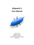
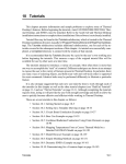
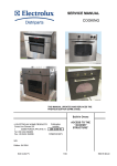
Analyze the heat conduction between concentric cylinders as shown in Figure 1-1. The
wall of the inner cylinder is kept fixed at 140oC while that of the outer cylinder is
exposed to an ambient at T = 20oC and the heat transfer coefficient is h = 1.5 W/cm2 -oC.
The thermal conductivity, k, of the material should be taken as 2 W/cm -oC in all
directions.
Governing Equations
This problem is governed by the steady state heat conduction equation:
k 2T Q 0 ,
where k is the thermal conductivity, T is temperature and Q is the volumetric heat
generation rate. Q is assumed to be zero for this problem.
CFD Type
This is a heat conduction problem. Therefore, the values of the u and v velocities should
be kept fixed during the solution stage. There are also no scalars to solve for this
problem. This problem will be solved in dimensional form. That is, Type 3 solution
method will be employed in the Solver (refer to the Users manual). We shall also take
advantage of the spatial symmetry of the problem. Consequently, our computational
model will be as shown below:
y
T = 20oC
h = 1.5 W/cm2-oC
4 cm
1 cm
T = 20oC
h = 1.5 W/cm2oC
(0,
T
0
n
(0,
(0,
T = 140oC
(0,
x
k = 2 W/cmoC
T
0
n
T = 140oC
k = 2 W/cmoC
(0, -4)
(a) Physical Domain
(b) Computational Model
Figure 1.1 Physical and Computational Domain for Sample Problem 1.
2 / 44
Initial Conditions
This problem will be analyzed as a transient one using the default initial conditions in
INSTED. The default initial conditions will be zero or the minimum Dirichlet boundary
conditions. If there are no Dirichlet conditions for a variable, INSTED sets the initial
condition to zero for that variable at every nodal point.
Boundary Conditions
Zero temperature gradient or
T
0
n
is specified on the symmetry boundary at x = 0. Temperature is specified as 140 oC on
the surface of the inner cylinder. A film coefficient boundary condition is used on the
surface of the outer cylinder. This boundary condition can be written as
k
T
h(T T ) q' '
n
However, INSTED expects the value of k∂T/∂n to be specified as opposed to -k∂T/∂n.
Thus,
k
T
h(T T ) q' '
n
Thus, the 4 heat flux parameters as discussed in Chapter 3 of the User Manual are:
P1 = -h = -1.5 W/cm2 -oC
P2 = 1
P3 = 20oC
P4 = 1
Computational Grid
This problem will be analyzed with an unstructured mesh consisting of 113 9-node
elements and 503 nodal points, including those at the centroids of the elements.
Project Files
The files required to reproduce the results reported here for this sample problem are:
Seger1.mes
Seger.cfd
Htflxmat.dat
Input data for use in Mesh Generator
Input data for CFD solver
Film coefficient boundary condition data
Location of Project Files
The project files above are located in the directory \insted30\cfd\samples.
3 / 44
Model Building and Mesh Generation
Refer to Section 2.3 of the User's Manual for description of the INSTED/CFD (2D) Mesh
Generation procedure. The status bar, Input Box, modeling tools, Main dialog box etc., are terms
that are described in the manuals.
The boundary of the model for this sample problem will be composed of two arcs and two lines.
These lines must form a counterclockwise loop in order to obtain the mesh of the area enclosed
by the loop. The steps for creating the mesh for the model are as follows:
1.
2.
3.
4.
Start INSTED/CFD (2D) Mesh Generator.
Click the New Project button on the Main dialog box.
Click the Limit button on the 'Controls' dialog box.
The 'Limits' dialog box appears.
Type in -6.5, 9.0, -5.0, 5.0 for the lower x, higher x, lower y and higher y screen limits in the
'Limits' dialog box.
5. Click the OK button to dismiss the 'Limits' dialog box.
To draw the two arc segments
6. Click the Arc icon from the Modeling Tools that reside on the Main dialog box.
Status bar displays the message: 'Pick Arc Center'.
7. Type in 0,1 in the Input Box and press Enter.
Status bar displays the message: 'Pick Arc Start Point'.
8. Type in 0,0 in the Input Box and press Enter.
Status bar displays the message: 'Pick Arc End Point'.
9. Type in 0,2 in the Input box and press Enter.
10. Repeat steps 5 to 8 using (0,0) for the second arc center and (0,-4), (0,4) for the start and end
points respectively.
To draw the two connecting lines
11. Click the Line icon from the Modeling Tools that reside on the Main dialog box.
Status bar displays the message: 'Pick 1st Point'.
12. Type in 0,4 in the Input Box and press Enter.
Status bar displays the message: 'Pick 2nd Point'
13. Type in 0,2 in the Input Box and press Enter.
14. Repeat Steps 10 to 12 using (0,0) and (0,-4) for the first and second points of the second line.
4 / 44
Notice that four lines have now been created up to this point. Line 1 is the smaller arc, while
Line 2 is the bigger arc, Line 3 is the straight line closer to the top of the screen while Line 4
is the second straight line. The lines are labelled in the display on the 'Graphics' dialog box.
Defining number of elements per line
15. Click the Line Properties button on the Main dialog box,
The 'Line Properties' dialog box appears.
16. Enter the values of 10, 20, 8, and 12 for the number of elements for lines 1, 2, 3, and 4
respectively as shown in the figure above. Press Enter after typing each value to move to the
next line.
17. Click the OK button to dismiss this dialog box.
Defining the area to mesh
18. Click the Edit Boundary button on the Main dialog box,
The 'Edit Boundary' dialog box appears. The dialog box indicates that four boundaries have
been created as shown in the 'Bdry' listbox.
19. Scroll through the boundaries created to find out the constituent lines by clicking the Next
button.
20. Exit the dialog box by clicking the OK button.
21. Click the Define Area button on the Main dialog box,
The 'Area Definition' dialog box appears. This is shown in the figure below except that the
first boundary is not yet inverted..
22. Click the Add button on this dialog box.
An area listed as '1' is added in the 'Area' listbox.
23. Click the first line of the 'Boundaries' listbox.
24. Type 1 and press Enter. This is meant to include boundary (made of Arc line 1) in this area,
25. Repeat Step 20 to include boundaries 2, 3, and 4 in the definition of the current area.
26. Click the first line of the 'Invert' listbox to reverse the direction of Arc Line 1 (You may have
realized from the order in which you entered coordinates (in Steps 6 through 14) that the arc
represented by line 1 has a clockwise orientation relative to the loop.) Your dialog box should
now be similar to the figure below.
27. Click the OK button to dismiss the 'Area Definition' dialog box.
5 / 44
Applying boundary conditions
28. Click the Line BC button on the Main dialog box,
Status bar displays message: 'Pick Side'.
29. Click the Line 1 on the graphics screen or type 1 and Press Enter in the Input Box
The 'Line BC' dialog box appears with the heading -"Boundary Condition, Side 1" (confirm
from the title of the dialog box that data is being received for Line 1. This will not be the case
if you accidentally selected some other line.).
30. Click the arrow for temperature and select the Dirichlet condition from the list.
An input box appears beside the boundary condition listbox once Dirichlet condition is
selected.
31. Enter a value of 140 in the input box.
32. Click the OK button to dismiss the dialog box.
33. Repeat this procedure for Line 2 but only click the Nusselt No. condition for this line, leaving
the remaining variables intact.
Mesh and Confirm Mesh Results
34. Click the Mesh button on the Main dialog box,
A mesh of the internal of our loop of lines is displayed on the 'Graphics' dialog box.
35. Click the Display button on the 'Controls' dialog box.
36. From the listbox, select 'Nusselt No.'
37. Click the Ok button on this dialog box to view nodes with Nusset number boundary
conditions.
38. Click the Refresh button twice on the 'Controls' dialog box to return the screen to it original
condition.
Note: You should have the same result as if you loaded the file 'seger1.mes' located in the
directory \insted30\cfd\samples\seger1.mes. You may also choose to save your current work.
Refer to the sections 'Loading a file' and 'Saving a file' in the first chapter of the Users Manual.
Obtaining a Solution to the Problem
39. Click the Solver button on the INSTED/CFD (2D) Mesh Generator Main dialog box.
The INSTED/CFD (2D)Solver program is launched. The mesh generated from the Mesh
Generation program is automatically loaded.
40. Click the Load Project button on the Main dialog box of the Solver program.
41. Type *.* in the filename field of the operating system 'Open File' dialog box that appears, and
press Enter.
A list of files in the current directory is displayed.
42. Locate the file 'Seger.cfd' from the 'Samples' directory.
43. Click this file and press Enter.
44. Click the Prob. Description button on the Main dialog box and inspect the loaded
parameters.
45. Click the OK button to dismiss the 'Prob. Description' dialog box.
46. Click the Material Properties button on the Main dialog box and inspect the loaded material
properties. Note particularly the heat flux parameters.
47. Click the OK button to dismiss the 'Material Properties' dialog box.
48. Click the Solve button on the Main dialog box
Program begins to generate a solution to the problem. The graphic screen is converted to one
that displays the status of the solution process.
49. Wait for the solution to complete.
6 / 44
Analyzing the Result
(Refer to the User's Manual for general details about INSTED/CFD (2D) Post-Processing.)
50. Click the Post Processor button on the INSTED/CFD (2D) Solver Main dialog box.
The INSTED/CFD (2D) Post-processor program is launched. The results from the
INSTED/CFD (2D) Solver are automatically loaded.
51. Click the Display button on the 'Controls' dialog box.
The 'Display' dialog box appears.
52. Select the most recent print step for viewing from the 'Time Step' listbox.
53. Click the Ok button to dismiss the 'Display' dialog box.
54. View the Contour Plot of Temperature.
55. Locate and open the file 'lola.out' in the working directory (\cfd for the current example).
56. Inspect and compare the values at selected nodal points.
Table 1.1 Heat Conduction Between Two Cylinders, with Film Coefficient Boundary Conditions
x-coord
0.0
0.0
0.0
0.0
0.0
1.0
0.707
4.0
y-coord
-2.0
-4.0
2.0
3.0
4.0
1.0
0.293
0.0
Segerlind
68.97
36.58
140
88.48
55.71
140
140
42.35
INSTED
67.70
36.22
140
87.10
55.36
140
140
42.10
Difference
<2%
<1%
<1%
<2%
<1%
<1%
<1%
<1%
File: lola.out
7 / 44
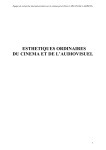
Number of nodes = 503
Number of 9 -node elements = 113
(a) Computational Model
(b) Contour Plot of Temperature
Figure 1.2 Mesh and temperature plot for Sample Problem 1.
Reference:
Segerlind, L. J., 1984. Applied Finite Element Analysis. Second Edition. John Wiley &
Sons, Ltd. New York. 405-408.
8 / 44
TEST PROBLEM 2
HEAT CONDUCTION WITH VOLUMETRIC HEAT SOURCE
Problem Statement
Analyze the time-dependent equation
T
2T 1 ,
t
{( x, y) : 0 ( x, y) 1
subject to the boundary conditions, for t 0,
T 0 on lines x 1 and y 1
T
0 on lines x 0 and y 0
n
and the initial boundary conditions for (x, y) in W
T=0;t=0
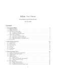
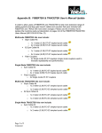
Physical and Computational Domain
The physical and computational domain is shown below:
y
T=0
1.0
T=0
T
0
n
x
1.0
Figure 2.1 Physical and Computational Domain
Governing Equations
This is written above as part of the problem statement.
9 / 44
Initial Condition
The problem will be analyzed as a transient one, for which the initial condition, T = 0, is
used everywhere. This is also the default initial condition in INSTED for this problem.
Boundary Conditions
This is written above as part of the problem statement.
Computational Grid
This test problem will be analyzed with a mesh consisting of 64 9-node elements and 289
nodal points, including the nodes at the centroids of the elements.
Project Files
The files required to reproduce our results for this sample problem are:
reddy.mes
reddy.cfd
Input data for use in Mesh Generator to generate mesh
Input data for CFD solver
Location of Project Files
The project files above are located in the directory \insted30\cfd\samples.
CFD Type
This is a transient heat conduction problem. Therefore, the velocities are not solved.
There are also no scalars. Since this problem is posed in terms of non-dimensional
parameters, one could in principle analyze this problem using CFD Type 1 or Type 2.
However, the temperature equation for this problem resembles the form in CFD Type 1 if
k = H = 1 (H is non-dimensional volumetric heat source). Moreover, for Type 2, it is not
clear what Re value must be used to obtain the right temperature equation and at the same
time ensure a motionless state. The reason for this is the appearance of the Peclet number
Pe = RePr, in the temperature equation for CFD Type 2. We have selected CFD Type 1
for this problem to avoid any ambiguities.
Model Building and Mesh Generation
Refer to INSTED/CFD (2D) manual for the description of the INSTED Mesh Generation GUI.
The status bar, Input Box, modeling tools, Main dialog box are discussed in the manuals.
The INSTED model for this sample problem is a square in which the four enclosing lines are
oriented in a counter-clockwise sense. The rectangle modeling tool in INSTED will be used to
produce a square with counter-clockwise orientation. The steps for generating the mesh for the
sample problem are as follows:
1. Start INSTED/CFD (2D) Mesh Generator. Skip this step if the program is already open.
However, you should close other INSTED/CFD (2D) programs that may have been opened
through the Mesh Generator.
10 / 44
2.
3.
4.
Click the New Project button on the Main dialog box.
Click the Limit button on the 'Controls' dialog box.
The 'Limits' dialog box appears.
Type in -0.2, 1.2, -0.2, 1.2 for the lower x, higher x, lower y and higher y screen limits in the
'Limits' dialog box.
5. Click the OK button on the 'Limits' dialog box.
To draw the square
6. Click the Rectangle tool button among the Modeling Tools that reside on the Main dialog
box.
Status bar displays the message: 'Pick 1st Corner Point'.
7. Type in 0,0 in the Input box and press Enter.
Status bar displays the message: 'Pick 2nd Corner Point'
8. Type in 1,1 in the Input box and press Enter.
Defining number of elements per line
9. Click the Line Properties button on the Main dialog box,
The 'Line Properties' dialog box appears.
10. Enter the values of 8, 8, 8, and 8 for the number of elements for lines 1, 2, 3, and 4
respectively. Press Enter after typing each value to move to the next line I the listbox.
11. Click the OK button to dismiss this dialog box.
Defining the area to mesh
12. Click the Define Area button on the Main dialog box,
The 'Area Definition' dialog box appears.
13. Click the Add button on this dialog box.
An area listed as '1' is added in the 'Areas' listbox.
14. Click the first line of the 'Boundaries' listbox.
15. Type 1 and press Enter. This is meant to include boundary 1 (made of Rectangle with lines
1,2,3, and 4) in this area,
16. Click the OK button to dismiss the 'Area Definition' dialog box.
Applying boundary conditions
17. Click the Line BC button on the Main dialog box,
Status bar displays message: 'Pick Side'.
18. Click the Line 3 on the graphics screen or type 3 and Press Enter in the Input Box
The 'Line BC' dialog box appears with the heading -"Boundary Condition, Side 3" (confirm
from the title of the dialog box that data is being received for Line 3. This will not be the case
if you accidentally selected some other line.).
19. Click the temperature boundary condition listbox's drop-down arrow and select the Dirichlet
condition from the list.
An input box appears beside the boundary condition listbox once Dirichlet condition is
selected.
20. Enter a value of 0 in the input box.
21. Click the OK button to dismiss the dialog box.
22. Repeat this procedure for Line 2.
Mesh and Confirm Mesh Results
23. Click the Mesh button on the Main dialog box,
A mesh of the internal of our loop of lines is displayed on the 'Graphics' dialog box.
24. Click the Display button on the 'Controls' dialog box.
25. From the listbox, select 'Dirichlet, Temp'
26. Click the Ok button on this dialog box to view nodes with Dirichlet temperature boundary
conditions.
11 / 44
27. Click the Refresh button twice on the 'Controls' dialog box to return the screen to it original
condition.
Note: You should have the same result as if you loaded the file \insted30\cfd\samples\reddy.mes.
You may also choose to save your current work. In this case, refer to the sections 'Loading a file'
and 'Saving a file' in the first chapter of the Users Manual.
Obtaining a Solution to the Problem
28. Click the Solver button on the Main dialog box.
The INSTED Solver program is launched. The mesh generated from the Mesh Generation
program is automatically loaded.
29. Click the Load Project button on the Main dialog box of the Solver program.
30. Type *.* in the filename section of the operating system Open File' dialog box that appears,
and press Enter.
A list of files in the current directory is displayed.
31. Locate the file 'reddy.cfd' from the 'Samples' directory.
32. Click this file and press Enter.
33. Click the Prob. Description button on the Main dialog box and inspect the loaded
parameters.
34. Click the OK button to dismiss the 'Prob. Description' dialog box.
35. Click the Material Properties button on the Main dialog box and inspect the loaded material
properties. Note particularly the heat flux parameters.
36. Click the OK button to dismiss the 'Material Properties' dialog box.
37. Click the Solve button on the Main dialog box
Program begins to generate a solution to the problem. The graphic screen is converted to one
that displays the status of the solution process.
38. Wait for the solution to complete.
Analyzing the Result
(Refer to the User's Manual for general details about INSTED/CFD (2D) Post-Processing.)
39.
40.
41.
42.
43.
44.
45.
Click the Post Processor button on the Main dialog box.
The INSTED Postprocessor program is launched. The results from the
Click the Display button on the 'Controls' dialog box.
The 'Display' dialog box appears.
Select the most recent time step for viewing from the 'Time Step' listbox.
Click the Ok button to dismiss the 'Display' dialog box.
View the Contour Plot of Temperature.
Locate and open the file 'lola.out' in the working directory (\cfd for the current example).
Inspect and compare the values at selected nodal points.
12 / 44
Table 1.1 Comparison of Results with Source
x-coord
0.0
0.0
0.0
0.0
0.0
File: lola.out
y-coord
0.0
0.25
0.5
0.75
1.0
Exact Solution
0.2947
0.2789
0.2293
0.1397
0.0
INSTED
0.2947
0.2789
0.2293
0.1397
0.0
Difference
<1%
<1%
<1%
<1%
<1%
Number of nodes = 289
Number of 9-node elements = 64
Figure 1.2 Mesh and temperature plot for Sample Problem 1.
Reference:
Reddy, J. N., 1984. An Introduction to the Finite Element Method. McGraw Hill Book
Co. New York. 303-305.
13 / 44
14 / 44
TEST PROBLEM 3
AXISYMETRIC CONDUCTION IN A CYLINDER
Problem Statement
Consider a cylinder of height L = 0.02 m, radius r = 0.01m, thermal conductivity k =
25W/cmoC and constant internal heat generation Q''' = 5 x 10⁸ W/m3. The top and bottom
faces and the curved surface of the cylinder are maintained at T0 = 100oC. Calculate the
axisymmetric temperature distribution in the (r, z) plane of the cylinder.
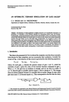
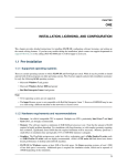
Physical and Computational Domain
The physical domain is shown in Fig. 3.1 (a)
(0.0, 0.0)
T/n = 0
(0.0, 0.01)
y
T/n = 0
T = 100oC
(0.01, 0.0)
T = 100oC
(0.01, 0.01)
x
(b)
(a)
Figure 3.1 Physical Domain for the Axisymetric Conduction Problem
The computational model is shown in Fig. 3.1 (b).
Governing Equations
The present sample problem is a conduction one with the equation
1 T 2T
k
r
2 Q' ' ' 0
r r r z
where k = 25W/cmoC is the thermal conductivity and Q''' = 5 x 10⁸ W/m3 is the
volumetric heat generation. The coordinates (r, z) ≡ (y, x) are the radial and axial
coordinates, respectively.
14 / 44
You must specify the axial coordinate (z) as the x- coordinate in INSTED and the radial
coordinate as the y- coordinate. This is the convection for axisymmetrical problems in
INSTED.
CFD Type
This problem will be solved as CFD Type 3; that is, without non-dimensionalization. We
will also take advantage of symmetry to simplify the problem. As a result, the
computational domain shown above was derived based on symmetry along the r- and zaxis.
Initial Condition
The problem will be analyzed as a transient one, for which the initial condition, T = 0, is
used everywhere. This is also the default initial condition in INSTED.
Boundary Conditions
This is illustrated in Figure 3.1 (b) and summarized below:
T
0
n
x 0.01 : T 100 0 C
T
y 0:
0
n
y 0.01 : T 100 0 C
x 0:
Also note that there is additional heat generation Q''' = 5 x 10⁸ W/m3.
Computational Grid
This problem will be analyzed with an unstructured mesh consisting of 25 9-node
elements and 121 nodal points, including those at the centroids of the elements.
Project Files
The files required to reproduce our results for this sample problem are:
axiscond.mes
axiscond.cfd
Input data for use in Mesh Generator to generate mesh
Input data for CFD solver
Location of Project Files
The project files above are located in the directory \insted30\cfd\samples.
Model Building and Mesh Generation
The model for this sample problem will be composed of a square with a counter-clockwise
orientation. The rectangle modeling tool in INSTED will be used to produce the square.
15 / 44
1.
2.
3.
4.
Start INSTED/CFD (2D) Mesh Generator.
Click the New Project button on the Main dialog box.
Click the Limit button on the 'Controls' dialog box.
The 'Limits' dialog box appears.
Type in -0.002, 0.012, -0.002, 0.012 for the lower x, higher x, lower y and higher y screen
limits in the 'Limits' dialog box.
5. Click the OK button to dismiss this dialog box.
To draw the square
6. Click the Rectangle tool button among the Modeling Tools that reside on the Main dialog
box.
Status bar displays the message: 'Pick 1st Corner Point'.
7. Type in 0,0 in the Input box and press Enter.
Status bar displays the message: 'Pick 2nd Corner Point'
8. Type in 0.01,0.01 in the Input box and press Enter.
Defining number of elements per line
9. Click the Line Properties button on the Main dialog box,
The 'Line Properties' dialog box appears.
10. Enter the values of 5, 5, 5, and 5 for the number of elements for lines 1, 2, 3, and 4
respectively. Press Enter after typing each value to move to the next line I the listbox.
11. Click the OK button to dismiss this dialog box.
Defining the area to mesh
12. Click the Define Area button on the Main dialog box,
The 'Area Definition' dialog box appears.
13. Click the Add button on this dialog box.
An area listed as '1' is added in the 'Areas' listbox.
14. Click the first line of the 'Boundaries' listbox.
15. Type 1 and press Enter. This is meant to include boundary (made of Rectangle with lines
1,2,3, and 4) in this area,
16. Click the OK button to dismiss the 'Area Definition' dialog box.
Applying boundary conditions
17. Click the Line BC button on the Main dialog box,
Status bar displays message: 'Pick Side'.
18. Click the Line 2 on the graphics screen or type 2 and Press Enter in the Input Box
The 'Line BC' dialog box appears with the heading -"Boundary Condition, Side2" (confirm
from the title of the dialog box that data is being received for Line 2. This will not be the case
if you accidentally selected some other line.).
19. Click the drop down list box for temperature and select a Dirichlet boundary condition from
the list and enter a value of 100.0 in the accompanying Input box that appears as soon as
Dirichlet condition is selected.
20. Click the OK button to dismiss the dialog box.
21. Repeat the procedure (17-20) for Line 3.
Mesh and Confirm Mesh Results
22. Click the Mesh button on the Main dialog box,
A mesh of the internal of our loop of lines is displayed on the 'Graphics' dialog box.
23. Click the Display button on the 'Controls' dialog box.
24. From the listbox, select 'Dirichlet, Temp'
25. Click the Ok button on this dialog box to view nodes with Dirichlet temperature boundary
conditions.
26. Click the Refresh button on the 'Controls' dialog box to return the screen to it original
condition.
16 / 44
Note: You should have the same result as if you loaded the file
\insted30\cfd\samples\axiscond.mes. You may also choose to save your current work. In this case,
refer to the sections 'Loading a file' and 'Saving a file' in the first chapter of the Users Manual.
Obtaining a Solution to the Problem
27. Click the Solver button on the INSTED/CFD (2D) Mesh Generator Main dialog box.
The INSTED/CFD (2D) Solver program is launched. The mesh generated from the Mesh
Generation program is automatically loaded.
28. Click the Load Project button on the Main dialog box of the Solver program.
29. Type *.* in the filename section of the operating system 'Open File' dialog box that appears,
and press Enter.
A list of files in the current directory is displayed.
30. Locate the file 'axiscond.cfd' from the 'Samples' directory.
31. Click this file and press Enter.
32. Click the Prob. Description button on the Main dialog box and inspect the loaded
parameters.
33. Click the OK button to dismiss the 'Prob. Description' dialog box.
34. Click the Material Properties button on the Main dialog box and inspect the loaded material
properties. Note particularly the heat flux parameters.
35. Click the OK button to dismiss the 'Material Properties' dialog box.
36. Click the Solve button on the Main dialog box
Program begins to generate a solution to the problem. The graphic screen is converted to one
that displays the status of the solution process.
37. Wait for the solution to complete.
Analyzing the Result
(Refer to the User's Manual for general details about INSTED/CFD (2D) Post-Processing.)
38.
39.
40.
41.
42.
43.
44.
Click the Post Processor button on the INSTED/CFD (2D) Solver Main dialog box.
The INSTED/CFD (2D) Post-processor program is launched. The results from the
Click the Display button on the 'Controls' dialog box.
The 'Display' dialog box appears.
Select the most recent time step for viewing from the 'Time Step' listbox.
Click the Ok button to dismiss the 'Display' dialog box.
View the Contour Plot of Temperature.
Locate and open the file 'lola.out' in the working directory (\cfd for the current example).
Inspect and compare the values at selected nodal points.
17 / 44
Table 3.1 Comparison of Results
r (z = 0.009)
0.000
0.001
0.002
0.003
0.004
0.005
0.006
0.007
0.008
0.009
0.010
Reddy
195.86
195.03
193.06
189.78
185.07
178.74
170.50
159.91
146.20
127.81
100.0
INSTED
195.21
194.96
192.68
189.44
184.73
178.40
170.12
159.50
145.62
127.23
100.0
Difference
<1%
<1%
<1%
<1%
<1%
<1%
<1%
<1%
<1%
<1%
<1%
r (z = 0.0)
0.000
0.001
0.002
0.003
0.004
0.005
0.006
0.007
0.008
0.009
0.010
Reddy
504.64
499.82
488.52
469.93
443.70
409.43
366.68
314.92
253.61
182.16
100.0
INSTED
501.30
497.70
486.81
468.50
442.49
408.43
365.88
314.33
253.22
181.97
100.0
Difference
<1%
<1%
<1%
<1%
<1%
<1%
<1%
<1%
<1%
<1%
<1%
Reference:
Reddy, J. N. & Gartling, D. K. (1994). The Finite Element Method in Heat Transfer and Fluid
Dynamics. CRC Press, Boca Raton, Florida, USA. 69-70.
18 / 44
TEST PROBLEM 4
PRESSURE DISTRIBUTION IN A VISCOUS FLOW OF A LUBRICANT BEARING
Problem Statement
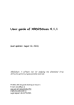
Calculate the pressure distribution in a lubricant flowing inside a slider bearing (Figure
4.1). The slider bearing consists of a short sliding pad moving at a velocity u = U = 30
relative to a stationary pad inclined at a small angle with respect to the stationary pad, as
the small gap between the two pads is filled with a lubricant. Since the ends of the
bearing are generally open, the pressure there is atmospheric, which will be taken as zero.
The pressure distribution inside the bearing is, in general, a function of x and y, and is set
up in the gap.
An exact solution, assuming that the pressure does not vary in y, can be shown as:
P
6U 0 (h2 h1 )(h h1 )
h 2 (h22 h12 )
1 2 dP y
1
u U 0
h
2
dx h
xy
y
h
U
u dP
h
y 0
y dx
2
h
h( x) h2
h2 h1
x
L
CFD Type
This problem will be solved as CFD Type 3; that is, in the dimensional form.
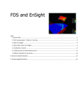
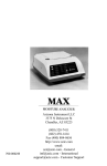
Physical and Computational Domain
The physical domain is shown in the figure below:
In the figure, h2 = 2h1 = 8 x 10⁻⁴, L = 0.36, = 8 x 10⁻⁴, U0 = 30, = 1.
Caution: You should be aware of the large aspect ratio of the physical system under
consideration. This quantity is equal to L/h1 = 900. Under this condition, the truly
automatic mesh generation method in INSTED defaults to the standard structured mesh
generation approach.
19 / 44
y
Slide block ( u = v = 0)
h2
P = P0
h(x)
P = P0
h1
U = 30 m/s
Guide Surface ( u = U0; v = 0)
Figure 4.1 Physical domain for the bearing problem
The computational domain will have the same orientation and dimensions as the physical
domain shown in this figure.
Computational Grid
This problem will be analyzed with an unstructured mesh consisting of 60 9-node
elements and 347 nodal points, including those at the centroids of the elements.
Governing Equations
The governing equations for CFD Type 3: Engineering CFD, are used on the assumption
that the data is given in dimensional quantities. (Note that no units have been specified.)
Isothermal flow conditions are assumed. The governing equations are:
u 0
u
1 p 1
u u
(u (u) * ) x
t
0 x 0
v
1 p 1
u v
(u (u) * ) y
t
0 y 0
Initial Condition
The default initial conditions in INSTED as described in Sample Problem 1 is used for
this problem. That is, u (x, y, 0) = v (x, y, 0) = 0.
Boundary Conditions
The appropriate boundary conditions for this sample problem is as follows:
Left (x = 0): tx = ty = 0
Right (x = 36): tx = ty = 0
20 / 44
Bottom (y = 0): u = 30, v = 0
Top: u = 0, v = 0
Project Files
The files required to reproduce our results for this sample problem are:
slider1.mes
slider.cfd
Input data for use in Mesh Generator
Input data for CFD solver
Location of Project Files
The project files above are located in the directory \insted30\cfd\samples.
Model Building and Mesh Generation
The CFD model for this sample problem will be generated using a structured mesh generation
procedure consisting of eight sides. The New Block modeling tool in INSTED will give us a
structured block. Note that the points of the block must be entered also in a counter-clockwise
direction. This is illustrated in the instructions below.
1.
2.
3.
4.
Start INSTED/CFD (2D) Mesh Generator.
Click the New Project button on the Main dialog box.
Click the Limit button on the 'Controls' dialog box.
The 'Limits' dialog box appears.
Type in -0.02, 0.4, -0.0002, 0.001 for the lower x, higher x, lower y and higher y screen limits
in the 'Limits' dialog box.
5. Click the OK button to dismiss this dialog box.
To draw the object
6. Click the New Boundary button on the Main dialog box.
Status bar displays the message: 'Pick Point 1'.
7. Type in 0,0 in the Input box and press Enter.
Status bar displays the message: 'Pick Point 2'
8. Type in 0.18,0.0 in the Input box and press Enter.
9. Type in 0.36,0.0 in the Input box and press Enter.
10. Type in 0.36, 2.0E-04 in the Input box and press Enter.
11. Type in 0.36, 4.0E-04 in the Input box and press Enter.
12. Type in 0.18, 4.0E-04 in the Input box and press Enter.
13. Type in 0.0, 8.0E-04 in the Input box and press Enter.
14. Type in 0.0, 4.0E-04 in the Input box and press Enter.
15. Type in 0.0,0.0 in the Input box and press Enter.
The slider shape as illustrated in the Figure 4.1 is obtained.
Defining number of elements per line
16. Click the Line Properties button on the Main dialog box,
The 'Line Properties' dialog box appears.
17. Enter the values of 9, 3, 9, and 3 for the number of elements for lines 1, 2, 3, and 4
respectively. Press Enter after typing each value to move to the next line I the listbox.
18. Click the OK button to dismiss this dialog box.
21 / 44
Defining the area to mesh
19. Click the Define Area button on the Main dialog box,
The 'Area Definition' dialog box appears.
20. Click the Add button on this dialog box.
An area listed as '1' is added in the 'Areas' listbox.
21. Click the first line of the 'Boundaries' listbox.
22. Type 1 and press Enter. This is meant to include boundary (made of Rectangle with lines
1,2,3, and 4) in this area,
23. Click the OK button to dismiss the 'Area Definition' dialog box.
Applying boundary conditions
24. Click the Line BC button on the Main dialog box,
Status bar displays message: 'Pick Side'.
25. Click the Line 1 on the graphics screen or type 1 and Press Enter in the Input Box
The 'Line BC' dialog box appears with the heading -"Boundary Condition, Side1" (confirm
from the title of the dialog box that data is being received for Line 1. This will not be the case
if you accidentally selected some other line.).
26. Click the drop down list box for u-velocity and select a Dirichlet boundary condition from the
list and enter a value of 30.0 in the accompanying Input box that appears as soon as Dirichlet
condition is selected.
27. Click the drop down list box for v-velocity and select a Dirichlet boundary condition from the
list and enter a value of 0.0 in the accompanying Input box that appears as soon as Dirichlet
condition is selected.
28. Click the OK button to dismiss the dialog box.
29. Repeat the procedure (20-24) for Line 3 setting Dirichlet conditions for u-velocity and vvelocity with values 0.0 and 0.0 respectively.
Mesh and Confirm Mesh Results
30. Click the Mesh button on the Main dialog box,
A mesh of the internal of our loop of lines is displayed on the 'Graphics' dialog box.
31. Click the Display button on the 'Controls' dialog box.
32. From the listbox, select 'Dirichlet, Temp'
33. Click the Ok button on this dialog box to view nodes with Dirichlet temperature boundary
conditions.
34. Click the Refresh button on the 'Controls' dialog box to return the screen to it original
condition.
Turning on Node & Element Numbering
35. Click the Display button on the 'Controls' dialog box.
The 'Display' dialog box appears
36. Click the 'Display Node Numbers' radio button to turn on display of node numbers
37. Click the 'Display Element Numbers' radio button to turn on display of node numbers
38. Click the OK button to dismiss the dialog box.
Note: You should have the same result as if you loaded the file \insted30\cfd\samples\slider.mes.
You may also choose to save your current work. Refer to the sections 'Loading a file' and 'Saving
a file' in the first chapter of the Users Manual.
Obtaining a Solution to the Problem
39. Click the Solver button on the INSTED/CFD (2D) Mesh Generator Main dialog box.
22 / 44
The INSTED/CFD (2D) Solver program is launched. The mesh generated from the Mesh
Generation program is automatically loaded.
40. Click the Load Project button on the Main dialog box of the Solver program.
41. Type *.* in the filename section of the operating system 'Open File' dialog box that appears,
and press Enter.
A list of files in the current directory is displayed.
42. Locate the file 'slider.cfd' from the 'Samples' directory.
43. Click this file and press Enter.
44. Click the Prob. Description button on the Main dialog box and inspect the loaded
parameters.
45. Click the OK button to dismiss the 'Prob. Description' dialog box.
46. Click the Material Properties button on the Main dialog box and inspect the loaded material
properties. Note particularly the heat flux parameters.
47. Click the OK button to dismiss the 'Material Properties' dialog box.
48. Click the Solve button on the Main dialog box
Program begins to generate a solution to the problem. The graphic screen is converted to one
that displays the status of the solution process.
49. Wait for the solution to complete.
Analyzing the Result
(Refer to the User's Manual for general details about INSTED/CFD (2D) Post-Processing.)
50. Click the Post Processor button on the INSTED/CFD (2D) Solver Main dialog box.
The INSTED/CFD (2D) Post-processor program is launched. The results from the Solver is
automatically loaded (Note that the model does not appear clearly initially due to its high
aspect ratio.)
51. Click the Axis button on the 'Controls' dialog box.
The 'Axis' dialog box appears.
52. Enter a value of 1.2 for the x-scale.
53. Enter a value of 140 for the y-scale.
54. Click the Ok button to dismiss the dialog box.
55. Click the Display button on the 'Controls' dialog box.
The 'Display' dialog box appears.
56. Select the most recent time step for viewing from the 'Time Step' listbox.
57. Click the Ok button to dismiss the 'Display' dialog box.
58. View the Contour Plot of Pressure.
59. Locate and open the file 'lola.out' in the working directory (\cfd for the current example).
60. Inspect and compare the values at selected nodal points.
Comparison of INSTED Results with Analytical Solution
x-coordinate
0.0063
0.0132
0.0207
0.0375
0.0567
0.0783
Analytic Solution
472.46
989.65
1551.14
2804.01
4221.43
5785.07
INSTED Result
468.52
989.56
1551.10
2805.70
4224.40
5788.90
Difference
<1%
<1%
<1%
<1%
<1%
<1%
23 / 44
0.1023
0.1575
0.1887
0.2479
0.2775
0.3039
0.3471
0.3559
7462.06
10886.40
12367.20
13465.98
12627.14
10634.62
3477.632
1188.77
7466.00
10885.00
12357.00
13462.00
12627.00
10631.00
3465.40
1173.00
<1%
<1%
<1%
<1%
<1%
<1%
<1%
<1%
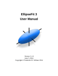
Figure 4.2 Computational Mesh of the Slider Problem
Figure 4.3 Plot of Pressure Contour for the Slider Problem
Reference:
Reddy, J. N. & Gartling, D. K. (1994). The Finite Element Method in Heat Transfer and
Fluid Dynamics. CRC Press, Boca Raton, Florida, USA. 69-70.
24 / 44
TEST PROBLEM 5
FLUID SQUEEZED BETWEEN PARALLEL PLATES
Problem Statement
The problem being considered is the (Stokes) flow of a viscous incompressible material
squeezed between two long parallel plates. A plane flow (in the plane formed by the
width of and the distance between the plates) is considered. Although this is a moving
boundary problem, we wish to determine the velocity and pressure fields for a fixed
distance between the plates, assuming that a state of plane flow exists. Results are
compared with Penalty and mixed formulations (Reddy and Gartling, 1994) as well as
with series solutions by Nadai (1963).
CFD Type
This problem will be solved as a CFD Type 2, posing it in the non-dimensional units. We
will also take advantage of symmetry in the x- and y- directions.
Physical and Computational Domain
The physical and computational domain are shown below:
(0, 2)
y
x
(6, 2)
ty = 0; tx = 0
u = 0; ty = 0
(0, 0)
(a)
u = 0; v = -1
v = 0; tx = 0
(6, 0)
(b)
Figure 5.1 Physical (a) and Computational (b) model for the test problem on viscous flow
between parallel plates
Governing Equations
The governing equations are the same as those presented in the main CFD manual for
CFD Type 2: Forced/Mixed Convection except that the present case is isothermal and the
Reynolds number is very small. This problem will be solved in an inertial frame since
there is no rotation of the system. The resulting equations are:
u 0,
u
p 1
u u
(u (u) * ) x ,
t
x Re
25 / 44
v
p 1
u v
(u (u) * ) y ,
t
y Re
Rer = Rar = 0,
where (u, v) are the velocities in the coordinate directions, and is the non-dimensional
value of the absolute viscosity. The Reynolds number, Re, is arbitrarily takes as 0.001,
consistent with Stokes flow requirement, = 1 and Pr is arbitrarily set to 7.0. The
mathematical symbols in these equations take on their usual meaning and are explained
in greater detail in the User's Manual.
Initial Condition
The default initial conditions in INSTED are used for this problem. That is, u (x, y, 0) = v
(x, y, 0) = 0.
Boundary Conditions
x = 0: u = 0, ty = 0
x = 6: tx = 0, ty = 0
y = 0: v = 0, tx = 0
y = 2: u = 0, v = -1
Project Files
The files required to reproduce our results for this sample problem are:
squeeze.mes
squeeze.cfd
Input data for use in Mesh Generator to generate mesh
Input data for CFD solver
Location of Project Files
The project files above are located in the directory \insted30\cfd\samples.
Model Building and Mesh Generation
The model for this sample problem will be composed of a square with a counter-clockwise
orientation. The rectangle modeling tool in INSTED will be used to produce the square.
1.
2.
3.
4.
Start INSTED/CFD (2D) Mesh Generator.
Click the New Project button on the Main dialog box.
Click the Limit button on the 'Controls' dialog box.
The 'Limits' dialog box appears.
Type in -0.5, 6.5, -0. 2, 2.2 for the lower x, higher x, lower y and higher y screen limits in the
'Limits' dialog box.
5. Click the OK button to dismiss this dialog box.
To draw the square
6. Click the Rectangle tool button among the Modeling Tools that reside on the Main dialog
box.
26 / 44
Status bar displays the message: 'Pick 1st Corner Point'.
7. Type in 0,0 in the Input box and press Enter.
Status bar displays the message: 'Pick 2nd Corner Point'
8. Type in 6, 2 in the Input box and press Enter.
Defining number of elements per line
9. Click the Line Properties button on the Main dialog box,
The 'Line Properties' dialog box appears.
10. Enter the values of 12, 4, 12, and 4 for the number of elements for lines 1, 2, 3, and 4
respectively. Press Enter after typing each value to move to the next line I the listbox.
11. Click the OK button to dismiss this dialog box.
Defining the area to mesh
12. Click the Define Area button on the Main dialog box,
The 'Area Definition' dialog box appears.
13. Click the Add button on this dialog box.
An area listed as '1' is added in the 'Areas' listbox.
14. Click the first line of the 'Boundaries' listbox.
15. Type 1 and press Enter. This is meant to include boundary 1 (made of Rectangle with lines
1,2,3, and 4) in this area.
16. Click the OK button to dismiss the 'Area Definition' dialog box.
Applying boundary conditions
17. Click the Line BC button on the Main dialog box,
Status bar displays message: 'Pick Side'.
18. Click the Line 3 on the graphics screen or type 3 and Press Enter in the Input Box
The 'Line BC' dialog box appears with the heading -"Boundary Condition, Side 3" (confirm
from the title of the dialog box that data is being received for Line 3. This will not be the case
if you accidentally selected some other line.).
19. Click the drop down list box for u-velocity and select a Dirichlet boundary condition from the
list and enter a value of 0.0 in the accompanying Input box that appears as soon as Dirichlet
condition is selected.
20. Click the drop down list box for v-velocity and select a Dirichlet boundary condition from the
list and enter a value of -1.0 in the accompanying Input box that appears as soon as Dirichlet
condition is selected.
21. Click the OK button to dismiss the dialog box.
22. Repeat the procedure (17-20) for Line 4 setting Dirichlet conditions only for u-velocity with a
value of 0.0.
23. Repeat the procedure (17-20) for Line 1 setting Dirichlet conditions only for v-velocity with a
value of 0.0.
Mesh and Confirm Mesh Results
24. Click the Mesh button on the Main dialog box,
A mesh of the internal of our loop of lines is displayed on the 'Graphics' dialog box.
25. Click the Display button on the 'Controls' dialog box.
26. From the listbox, select 'Dirichlet, Temp'
27. Click the Ok button on this dialog box to view nodes with Dirichlet temperature boundary
conditions.
28. Click the Refresh button on the 'Controls' dialog box to return the screen to it original
condition.
Note: You should have the same result as if you loaded the \insted30\cfd\samples\axiscond.mes.
You may also choose to save your current work. Refer to the sections 'Loading a file' and 'Saving
a file' in the first chapter of the Users Manual.
27 / 44
Obtaining a Solution to the Problem
29. Click the Solver button on the INSTED/CFD (2D) Mesh Generator Main dialog box.
The INSTED/CFD (2D) Solver program is launched. The mesh generated from the Mesh
Generation program is automatically loaded.
30. Click the Load Project button on the Main dialog box of the Solver program.
31. Type *.* in the filename section of the operating system 'Open File' dialog box that appears,
and press Enter.
A list of files in the current directory is displayed.
32. Locate the file 'squeeze.cfd' from the 'Samples' directory.
33. Click this file and press Enter.
34. Click the Prob. Description button on the Main dialog box and inspect the loaded
parameters.
35. Click the OK button to dismiss the 'Prob. Description' dialog box.
36. Click the Material Properties button on the Main dialog box and inspect the loaded material
properties. Note particularly the heat flux parameters.
37. Click the OK button to dismiss the 'Material Properties' dialog box.
38. Click the Solve button on the Main dialog box
Program begins to generate a solution to the problem. The graphic screen is converted to one
that displays the status of the solution process.
39. Wait for the solution to complete.
Analyzing the Result
(Refer to the User's Manual for general details about INSTED/CFD (2D) Post-Processing.)
40.
41.
42.
43.
44.
45.
46.
Click the Post Processor button on the INSTED/CFD (2D) Solver Main dialog box.
The INSTED/CFD (2D) Postprocessor program is launched. The results from the
Click the Display button on the 'Controls' dialog box.
The 'Display' dialog box appears.
Select the most recent time step for viewing from the 'Time Step' listbox.
Click the Ok button to dismiss the 'Display' dialog box.
View the Vector Plot for velocity.
Locate and open the file 'lola.out' in the working directory (\cfd for the current example).
Inspect and compare the values at selected nodal points.
28 / 44
Table 6.1 Comparison of Results
The velocities u(x) at y = 0 obtained from INSTED are compared in the table below with
those from the references.
x- coord
1.0
2.0
3.0
4.0
4.5
5.0
5.5
6.0
Series
Solution
Penalty
9-node
(Nadai)
(Reddy)
.7500
.7505
1.500
1.499
2.250
2.256
3.000
3.024
3.375
3.431
3.750
3.803
4.125
4.108
4.500
4.194
* Relation to the exact solution
Mixed
Model
9-node
(Reddy)
.7497
1.503
2.256
3.020
3.429
3.816
4.120
4.236
INSTED
12 x 4
Re = 0.001
.7500
1.502
2.256
3.026
3.422
3.811
4.135
4.243
Difference*
<1%
<1%
<1%
<1%
<1%
<2%
<1%
<6%
Figure 5.2 Vector Plot of Velocity for Fluid Squeezed Between Parallel Plates
Reference:
Reddy, J. N. & Gartling, D. K. (1994). The Finite Element Method in Heat Transfer and
Fluid Dynamics. CRC Press, Boca Raton, Florida, USA. 69-70.
Nadia, A. 1963. Theory of Flow and Fracture of Solids, Volume II. McGraw Hill, New
York.
29 / 44
TEST PROBLEM 6
NATURAL CONVECTION OF AIR IN A SQUARE CAVITY: A BENCHMARK
NUMERICAL SOLUTION
Problem Statement
The problem being considered is that of the two-dimensional flow of a Boussinesq fluid
of Prandtl number 0.71 in an upright square cavity of side L (L = 1 in non-dimensional
variables). Both velocity components are zero on all the boundaries. The horizontal walls
are insulated, and the left and right vertical sides are at temperatures Th and Tc,
respectively, which are 1 and 0 in non-dimensional units.
The solutions to this problem, namely, the velocities, the temperature and the rate of heat
transfer, are to be obtained for Rayliegh numbers, Ra = 104.
CFD Type
This problem will be solved as CFD Type 1; that is, using non-dimensional units for free
convection.
Physical and Computational Domain
The physical and computational domain are shown below:
u = v = = 0,
T/n = 0
u = v = = 0,
(1, 1)
u = v = = 0,
T=
0
T=
1
(0, 0)
u = v = = 0,
T/n = 0
Figure 6.1 Physical Domain for Natural Convection Problem
30 / 44
Governing Equations
The governing equations are the same as those presented in the main CFD manual for
CFD Type 1: Free Convection. However, this problem will be solved in an inertial frame,
the rotational terms in the equations have to be set to zero. That is:
Rer = Rar = 0.
The volumetric heat source, H, should also be set to zero, and you should take the ycoordinate as pointing in the negative direction of the normal gravity vector. The
governing equation can be written as
u 0
u
p
u u Pr (u (u) * ) x
t
x
v
p
u v Pr (u (u) * ) y Ra Pr T
t
y
T
u T kT
t
where (u, v) are the velocities in the x- and y-coordinate directions, and and k are the
non-dimensional value of the absolute viscosity and thermal conductivity respectively.
The Prandtl number, Pr, is taken as 0.71 while a Rayliegh number of 104 is used. The
mathematical symbols in these equations take on their usual meaning and are explained
in greater detail in the Users Manual.
Initial Condition
The default initial conditions in INSTED is used for this problem. That is, u (x, y, 0) = v
(x, y, 0) = 0.
Boundary Conditions
Two-dimensional flow of a Boussinesq fluid of Prandtl number 1, in an upright square
cavity is described in non-dimensional terms by
0 x 1,
0y1
with y vertically upwards. The problem assumes that both components of the velocity are
zero on all boundaries and the boundaries are y = 0 and y = 1 are insulate,
T
0,
n
and that T = 1 at x = 0 and T = 0 at x = 1.
31 / 44
Computational Grid
Two different mesh models are used - an 8 x 8 square mesh and a 10 x 10 boundary layer
mesh with 4 layers, 0.3 depth and a packing factor of 1.04. The 8 x 8 square is consists of
64 elements and 289 nodes including the nodes at the center while the boundary layer
mesh includes 81 elements and 361 nodes.
Project Files
The files required to reproduce our results for this sample problem are:
Devahl1.mes
Devahl2.mes
Devahl.cfd
Input data for 8 x 8 mesh of model
Input data for boundary layer mesh of model
Input data for CFD solver
Location of Project Files
The project files above are located in the directory \insted30\cfd\samples.
Model Building and Mesh Generation
The mesh boundary for this problem is a square with counter-clockwise orientation. The rectangle
modeling tool in INSTED will be used to produce the square. Details of mesh generation follow:
1.
2.
3.
4.
Start INSTED/CFD (2D) Mesh Generator.
Click the New Project button on the Main dialog box.
Click the Limit button on the 'Controls' dialog box.
The 'Limits' dialog box appears.
Type in -0.2, 1.2, -0. 2, 1.2 for the lower x, higher x, lower y and higher y screen limits in the
'Limits' dialog box.
5. Click the OK button to dismiss this dialog box.
To draw the square
6. Click the Rectangle tool button among the Modeling Tools that reside on the Main dialog
box.
Status bar displays the message: 'Pick 1st Corner Point'.
7. Type in 0,0 in the Input box and press Enter.
Status bar displays the message: 'Pick 2nd Corner Point'
8. Type in 1, 1 in the Input box and press Enter.
Defining number of elements per line
9. Click the Line Properties button on the Main dialog box,
The 'Line Properties' dialog box appears.
10. Enter the values of 8, 8, 8, and 8 for the number of elements for lines 1, 2, 3, and 4
respectively. Press Enter after typing each value to move to the next line I the listbox.
11. Click the OK button to dismiss this dialog box.
Defining the area to mesh
12. Click the Define Area button on the Main dialog box,
The 'Area Definition' dialog box appears.
13. Click the Add button on this dialog box.
An area listed as '1' is added in the 'Areas' listbox.
14. Click the first line of the 'Boundaries' listbox.
32 / 44
15. Type 1 and press Enter. This is meant to include boundary (made of Rectangle with lines
1,2,3, and 4) in this area,
16. Click the OK button to dismiss the 'Area Definition' dialog box.
Applying boundary conditions
17. Click the Line BC button on the Main dialog box,
Status bar displays message: 'Pick Side'.
18. Click the Line 1 on the graphics screen or type 1 and Press Enter in the Input Box
The 'Line BC' dialog box appears with the heading -"Boundary Condition, Side 1" (confirm
from the title of the dialog box that data is being received for Line 1. This will not be the case
if you accidentally selected some other line.).
19. Click the drop down list box for u-velocity and select a Dirichlet boundary condition from the
list and enter a value of 0.0 in the accompanying Input box that appears as soon as Dirichlet
condition is selected.
20. Click the drop down list box for v-velocity and select a Dirichlet boundary condition from the
list and enter a value of 0.0 in the accompanying Input box that appears as soon as Dirichlet
condition is selected.
21. Click the drop down list box for stream function and select a Dirichlet boundary condition
from the list and enter a value of 0.0 in the accompanying Input box that appears as soon as
Dirichlet condition is selected.
22. Click the OK button to dismiss the dialog box.
23. Repeat the procedure (17-21) for Line 3.
24. Click the Line BC button on the Main dialog box,
Status bar displays message: 'Pick Side'.
25. Click the Line 4 on the graphics screen or type 4 and Press Enter in the Input Box
The 'Line BC' dialog box appears with the heading -"Boundary Condition, Side 4" (confirm
from the title of the dialog box that data is being received for Line 4. This will not be the case
if you accidentally selected some other line.).
26. Click the drop down list box for u-velocity and select a Dirichlet boundary condition from the
list and enter a value of 0.0 in the accompanying Input box that appears as soon as Dirichlet
condition is selected.
27. Click the drop down list box for v-velocity and select a Dirichlet boundary condition from the
list and enter a value of 0.0 in the accompanying Input box that appears as soon as Dirichlet
condition is selected.
28. Click the drop down list box for stream function and select a Dirichlet boundary condition
from the list and enter a value of 0.0 in the accompanying Input box that appears as soon as
Dirichlet condition is selected.
29. Click the drop down list box for temperature and select a Dirichlet boundary condition from
the list and enter a value of 1.0 in the accompanying Input box that appears as soon as
Dirichlet condition is selected.
30. Click the radio button 'Nusset No. BC on Side' to indicate that you with to calculate the
Nusset number along this line.
31. Click the OK button to dismiss the dialog box.
32. Repeat the procedure (24-29) for Line 2 setting Dirichlet conditions for temperature with a
value of 0.0 while executing step 29.
33. Click the OK button to dismiss the dialog box.
Mesh and Confirm Mesh Results
34. Click the Mesh button on the Main dialog box,
A mesh of the internal of our loop of lines is displayed on the 'Graphics' dialog box.
35. Click the Display button on the 'Controls' dialog box.
36. From the listbox, select 'Dirichlet, Temp'
33 / 44
37. Click the Ok button on this dialog box to view nodes with Dirichlet temperature boundary
conditions.
38. Click the Refresh button on the 'Controls' dialog box to return the screen to it original
condition.
Note: You should have the same result as if you loaded the file
\insted30\cfd\samples\devahl1.mes. You may also choose to save your current work. Refer to the
sections 'Loading a file' and 'Saving a file' in the first chapter of the Users Manual.
Obtaining a Solution to the Problem
39. Click the Solver button on the INSTED/CFD (2D) Mesh Generator Main dialog box.
The INSTED/CFD (2D) Solver program is launched. The mesh generated from the Mesh
Generation program is automatically loaded.
40. Click the Load Project button on the Main dialog box of the Solver program.
41. Type *.* in the filename section of the operating system 'Open File' dialog box that appears,
and press Enter.
A list of files in the current directory is displayed.
42. Locate the file 'devahl1.cfd' from the 'Samples' directory.
43. Click this file and press Enter.
44. Click the Prob. Description button on the Main dialog box and inspect the loaded
parameters.
45. Click the OK button to dismiss the 'Prob. Description' dialog box.
46. Click the Material Properties button on the Main dialog box and inspect the loaded material
properties. Note particularly the heat flux parameters.
47. Click the OK button to dismiss the 'Material Properties' dialog box.
Selecting Sample Points for History Data
48. Click the Select Points button on the Main dialog box.
49. Select about eight nodal points by clicking the points on the graphics display
50. Click the Stop button on the Main dialog box to stop selecting points
51. Click the Solve button on the Main dialog box
Program begins to generate a solution to the problem. The graphic screen is converted to one
that displays the status of the solution process.
52. Wait for the solution to complete.
Analyzing the Result
(Refer to the User's Manual for general details about INSTED/CFD (2D) Post-Processing.)
53.
54.
55.
56.
57.
58.
59.
60.
61.
Click the Post Processor button on the INSTED/CFD (2D) Solver Main dialog box.
The INSTED/CFD (2D) Postprocessor program is launched. The results from the
Click the Display button on the 'Controls' dialog box.
The 'Display' dialog box appears.
Select the most recent time step for viewing from the 'Time Step' listbox.
Click the Ok button to dismiss the 'Display' dialog box.
View the Vector plot for velocity.
View the Contour plots for velocities, temperature, stream function, and pressure.
View the time-history data for the selected sample points.
Locate and open the file 'lola.out' in the working directory (\cfd for the current example).
Inspect and compare the values at selected nodal points.
34 / 44
Generating the Boundary Layer Mesh
62. Click the Line Properties button on the Main dialog box,
The 'Line Properties' dialog box appears.
63. Click the 'B.L' listbox for all four lines that form the boundary of the object.
The listbox should now have the text 'YES' on every line.
64. Click the OK button to dismiss this dialog box.
Specifying Boundary Layer Parameters
65. Click the Mesh Control button on the Main dialog box.
The 'Mesh Control' dialog box appears.
66. Click the radio button 'Boundary Layer Mesh' to indicate that you wish to generate a
boundary layer mesh.
67. Enter the values 4, 0.3 and 1.04 in the input boxes for the number of layers, depth, and
packing factor.
68. Click the OK button to dismiss this dialog box.
69. Repeat steps 34 through 61 for this mesh.
Table 6.1 Comparison of Results
||max
Umax
Vmax
Nu at left
Numax
Bench Mark
Results
5.071
16.178
19.617
2.238
3.528
INSTED
Results
5.074
16.2
19.6
2.23
3.53
Difference
<1%
<1%
<1%
<1%
<1%
INSTED
file
Psimax.out
Lola.out
Lola.out
Numean.out
Nusset.out
Figure 6.2 Vector Plot of Velocity for the Natural Convection Problem
35 / 44
What's Next?
After reproducing the results for this test problem, go through the exercise again but this
time, change the input data in the project file to study the effect on the solution. For
example, during mesh generation, you could change the number of elements in each of
the I and J directions. During analysis, you could locate the thermophysical properties,
dimensionless parameters, solution parameters, etc. and change them to study the effect
on the solutions.
Figure 6.3 Contour Plot of Temperature for the Natural Convection Problem
Reference:
Davis, G. de Vahl. (1983). Natural Convection in a Square Cavity. A comparison
Exercise. Int. J. Numerical Methods in Fluids. Volume 3. 227-248.
Davis, G. de Vahl. (1983). Natural Convection in a Square Cavity. A Benchmark
Numerical Solution. Int. J. Numerical Methods in Fluids. Volume 3. 249-264.
36 / 44
TEST PROBLEM 7
NATURAL CONVECTION TRANSPORT OF TEMPERATURE AND TWO NONREACTING SPECIES
Problem Statement
The problem being considered is that of the two-dimensional flow of a Boussinesq fluid
of Prandtl number 0.71 in an upright square cavity of side L (L = 1 in non-dimensional
variables). Both velocity components are zero on all the boundaries. The horizontal walls
are insulated, and the left and right vertical sides are at temperatures Th amd Tc,
respectively, which are 1 and 0 in non-dimensional units.
The natural convection flow is used to transport two chemical species (of different
diffusivities) within the box. It is assumed that bouyancy only results from temperature
differences. The solution at Ra = 104 is desired.
CFD Type
This problem will be solved as a CFD Type 1 posing the solution in the non-dimensional
units.
Physical and Computational Domain
The physical domain is as shown in Figure 6.1 except that we now have to include
passive scalars which we assume have the same boundary conditions as temperature.
Governing Equations
The governing equations are the same as those presented in the main CFD manual for
CFD Type 1: Free Convection. However, this problem will be solved in an inertial frame,
the rotational terms in the equations have to be set to zero. That is,
Rer = Rar = 0.
The volumetric heat source, H, should also be set to zero, and you should take the ycoordinate as pointing in the negative direction of the normal gravity vector. The
governing equation can be written as
u 0
u
p
u u Pr (u (u) * ) x
t
x
v
p
u v Pr (u (u) * ) y Ra Pr T
t
y
T
u T kT
t
37 / 44
P11 1 u 1 P121 P13
t
P21 2 u 2 P22 2 P23
t
where (u, v) are the velocities in the coordinate directions, and and k are the nondimensional value of the absolute viscosity and thermal conductivity respectively. The
parameters and k take on the values of 1 for the test problem. 1 and 2 represent the
concentrations of the two species to be calculated. Pij (i = 1, 2; j = 1, 2, 3) are the three
parameters (index j) for each of the two scalar equations (index i).
For this sample problem,
P11 = P21 = 1
P12 =25; P22 = 1
P13 = P23 = 0
The Prandtl number, Pr, is taken as 0.71 while the Rayliegh number is 104. The
mathematical symbols in these equations take on their usual meaning.
Initial Condition
The default initial conditions in INSTED is used for this problem. That is, u (x, y, 0) = v
(x, y, 0) = 1 (x, y, 0) = 2 (x, y, 0) = 0.
Boundary Conditions
Two-dimensional flow of Boussinesq fluid of Prandtl number 0.71, in an upright square
cavity is described in non-dimensional terms by
0 x 1,
0y1
with y vertically upwards. The problem assumes that both components of the velocity are
zero on all boundaries and the boundaries at y = 0 and y = 1 are insulated,
T
0,
n
and that T = 1 at x = 0 and T = 0 at x = 1. The boundary conditions on the scalars are the
same as those for temperature.
Computational Grid
An 8 x 8 square mesh of 9-node quadrilateral elements will be used. The total number of
64elements is and the total number of nodes including those at the centroid of elements is
289.
38 / 44
Project Files
The files required to reproduce our results for this sample problem are:
devscala.mes
devscala.cfd
Input data for 8 x 8 mesh of model
Input data for CFD solver
Location of Project Files
The project files above are located in the directory \insted30\cfd\samples.
Model Building and Mesh Generation
The mesh boundary for this problem is a square with counter-clockwise orientation. The rectangle
modeling tool in INSTED will be used to produce the square. Details of mesh generation follow:
1.
2.
3.
4.
Start INSTED/CFD (2D) Mesh Generator.
Click the New Project button on the Main dialog box.
Click the Limit button on the 'Controls' dialog box.
The 'Limits' dialog box appears.
Type in -0.2, 1.2, -0. 2, 1.2 for the lower x, higher x, lower y and higher y screen limits in the
'Limits' dialog box.
5. Click the OK button to dismiss this dialog box.
To draw the square
6. Click the Rectangle tool button among the Modeling Tools that reside on the Main dialog
box.
Status bar displays the message: 'Pick 1st Corner Point'.
7. Type in 0,0 in the Input box and press Enter.
Status bar displays the message: 'Pick 2nd Corner Point'
8. Type in 1, 1 in the Input box and press Enter.
Defining number of elements per line
9. Click the Line Properties button on the Main dialog box,
The 'Line Properties' dialog box appears.
10. Enter the values of 8, 8, 8, and 8 for the number of elements for lines 1, 2, 3, and 4
respectively. Press Enter after typing each value to move to the next line I the listbox.
11. Click the OK button to dismiss this dialog box.
Defining the area to mesh
12. Click the Define Area button on the Main dialog box,
The 'Area Definition' dialog box appears.
13. Click the Add button on this dialog box.
An area listed as '1' is added in the 'Areas' listbox.
14. Click the first line of the 'Boundaries' listbox.
15. Type 1 and press Enter. This is meant to include boundary (made of Rectangle with lines
1,2,3, and 4) in this area,
16. Click the OK button to dismiss the 'Area Definition' dialog box.
Entering the Number of Scalars
17. Click on the Scalars button on the Main dialog box.
The status bar displays the message - "Enter the number of scalars"
18. Enter a value of 2 in the Input box and press Enter.
39 / 44
Applying boundary conditions
19. Click the Line BC button on the Main dialog box,
Status bar displays message: 'Pick Side'.
20. Click the Line 1 on the graphics screen or type 1 and Press Enter in the Input Box
The 'Line BC' dialog box appears with the heading -"Boundary Condition, Side 1" (confirm
from the title of the dialog box that data is being received for Line 1. This will not be the case
if you accidentally selected some other line.).
21. Click the drop down list box for u-velocity and select a Dirichlet boundary condition from the
list and enter a value of 0.0 in the accompanying Input box that appears as soon as Dirichlet
condition is selected.
22. Click the drop down list box for v-velocity and select a Dirichlet boundary condition from the
list and enter a value of 0.0 in the accompanying Input box that appears as soon as Dirichlet
condition is selected.
23. Click the drop down list box for stream function and select a Dirichlet boundary condition
from the list and enter a value of 0.0 in the accompanying Input box that appears as soon as
Dirichlet condition is selected.
24. Click the OK button to dismiss the dialog box.
25. Repeat the procedure (19-23) for Line 3.
26. Click the Line BC button on the Main dialog box,
Status bar displays message: 'Pick Side'.
27. Click the Line 2 on the graphics screen or type 2 and Press Enter in the Input Box
The 'Line BC' dialog box appears with the heading -"Boundary Condition, Side 2" (confirm
from the title of the dialog box that data is being received for Line 2. This will not be the case
if you accidentally selected some other line.).
28. Click the drop down list box for u-velocity and select a Dirichlet boundary condition from the
list and enter a value of 0.0 in the accompanying Input box that appears as soon as Dirichlet
condition is selected.
29. Click the drop down list box for v-velocity and select a Dirichlet boundary condition from the
list and enter a value of 0.0 in the accompanying Input box that appears as soon as Dirichlet
condition is selected.
30. Click the drop down list box for stream function and select a Dirichlet boundary condition
from the list and enter a value of 0.0 in the accompanying Input box that appears as soon as
Dirichlet condition is selected.
31. Click the drop down list box for temperature and select a Dirichlet boundary condition from
the list and enter a value of 0.0 in the accompanying Input box that appears as soon as
Dirichlet condition is selected.
32. Click the drop down list box for scalar 1 (Scalar 1 is the scalar that is selected by default for
boundary condition input) and select a Dirichlet boundary condition from the list and enter a
value of 0.0 in the accompanying Input box that appears as soon as Dirichlet condition is
selected.
33. Change the selected scalar to Scalar 2 by clicking the drop down arrow of the Scalar listbox
and clicking on Scalar 2.
34. Click the drop down list box for Scalar 2 and select a Dirichlet boundary condition from the
list and enter a value of 0.0 in the accompanying Input box that appears as soon as Dirichlet
condition is selected.
35. Click the OK button to dismiss the dialog box.
36. Repeat the procedure (26-35) for Line 4 setting Dirichlet conditions for temperature with a
value of 1.0 while executing step 29.
Mesh and Confirm Mesh Results
37. Click the Mesh button on the Main dialog box,
40 / 44
38.
39.
40.
A mesh of the internal of our loop of lines is displayed on the 'Graphics' dialog box.
Click the Display button on the 'Controls' dialog box.
From the listbox, select 'Dirichlet, Temp'
Click the Ok button on this dialog box to view nodes with Dirichlet temperature boundary
conditions.
41. Click the Refresh button on the 'Controls' dialog box to return the screen to it original
condition.
Note: You should have the same result as if you loaded the file 'devscala.mes' in the Samples
directory of the \insted30\cfd\devscala.mes. You may also choose to save your current work.
Refer to the sections 'Loading a file' and 'Saving a file' in the first chapter of the Users Manual.
Obtaining a Solution to the Problem
42. Click the Solver button on the INSTED/CFD (2D) Mesh Generator Main dialog box.
The INSTED/CFD (2D) Solver program is launched. The mesh generated from the Mesh
Generation program is automatically loaded.
43. Click the Load Project button on the Main dialog box of the Solver program.
44. Type *.* in the filename section of the operating system 'Open File' dialog box that appears,
and press Enter.
A list of files in the current directory is displayed.
45. Locate the file 'devscala.cfd' from the 'Samples' directory.
46. Click this file and press Enter.
47. Click the Prob. Description button on the Main dialog box and inspect the loaded
parameters.
48. Click the OK button to dismiss the 'Prob. Description' dialog box.
49. Click the Material Properties button on the Main dialog box and inspect the loaded material
properties. Note particularly the heat flux parameters.
50. Click the OK button to dismiss the 'Material Properties' dialog box.
Analyzing the Result
(Refer to the User's Manual for general details about INSTED/CFD (2D) Post-Processing.)
51.
52.
53.
54.
55.
56.
Click the Post Processor button on the INSTED/CFD (2D) Solver Main dialog box.
The INSTED/CFD (2D) Postprocessor program is launched. The results from the
Click the Display button on the 'Controls' dialog box.
The 'Display' dialog box appears.
Select the most recent time step for viewing from the 'Time Step' listbox.
Click the Ok button to dismiss the 'Display' dialog box.
View the Vector plot for velocity.
View the Contour plots for velocities, temperature, stream function, scalars 1 & 2, and
pressure.
57. Locate and open the file 'lola.out' in the working directory (\cfd for the current example).
58. Inspect and compare the values at selected nodal points.
41 / 44
Results
The contour maps for temperature, and the three scalars are shown in Figures 7.1 through
7.3. Note the similarity in the results for temperature and scalar 2. Since the flow is
purely thermally driven, some differences, no matter how small should exist between
scalar 2 and temperature because of the closer tie between temperature and the velocity.
Finally, note that, because of the coarse grid used, unphysical solutions were observed.
While scalar 1 have a high diffusivity to dissipate unphysical results, scalar 2 and the
temperature do show the unphysical results because of low diffusivities.
What's Next?
After reproducing the results for this test problem, go through the exercise again but this
time, change the input data in the project file to study the effect on the solution. For
example, during mesh generation, you could change the number of elements in each of
the I and J directions. During analysis, you could locate the thermophysical properties,
dimensionless parameters, solution parameters, etc. and change them to study the effect
on the solutions.
Figure 7.1 Contour Plot of Temperature for the Test Problem on the Transport of
Temperature and Species By Natural Convection in a Cavity for Ra = 104.
42 / 44
Figure 7.2 Contour Plot of Scalar 1 for the Test Problem on the Transport of Temperature
and Species By Natural Convection in a Cavity for Ra = 104.
43 / 44
Figure 7.3 Contour Plot of Scalar 2 for the Test Problem on the Transport of Temperature
and Species By Natural Convection in a Cavity for Ra = 104.
Reference:
Davis, G. de Vahl. (1983). Natural Convection in a Square Cavity. A comparison
Exercise. Int. J. Numerical Methods in Fluids. Volume 3. 227-248.
Davis, G. de Vahl. (1983). Natural Convection in a Square Cavity. A Benchmark
Numerical Solution. Int. J. Numerical Methods in Fluids. Volume 3. 249-264.
44 / 44