Download RT-Lab Solo User`s Manual - Centre for Intelligent Machines

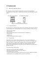
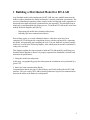
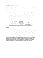
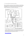
RT-Lab Solo
Getting Started User’s Manual
IA Lab
Center for Intelligent Machine
McGill University
Version: 1.0
Feb. 16, 03
1 Fundamental
1.1
How RT-LAB Solo Works
RT-LAB Solo runs on a hardware configuration consisting of Command Station,
Compilation Node, Target Node, Communication Links (real-time and Ethernet), and I/O
boards.
1.1.1 Command Station
RT-LAB software is configured on a Windows NT or Windows 2000 computer called the
Command Station. The Command Station serves as the user interface. It allows users to:
• Edit and modify models;
• See model data;
• Run the original model under its simulation software (Simulink etc.);
• Generate code;
• Separate code;
• Control the simulator's Go/Stop sequences.
1.1.2 Target Node
Target Node is the computer where simulation runs. For real-time simulation, the
preferred operating system for the Target Node is QNX. When there are multiple QNX
nodes, one of them is assigned as the Compilation Node. The Command Station and
Target Node(s) communicate with each other using communication links, and for
hardware-in-the-loop simulations Target Node may also communicate with other devices
through I/O boards.
The real-time Target Node perform:
• Real-time execution of the model’s simulation;
• Real-time communication between the nodes and I/Os;
• Initialization of the I/O systems;
• Acquisition of the model’s internal variables and external outputs through I/O modules;
• Implementation of user-performed online parameters modification;
2
• Recording data on local hard drive, if desired;
• Supervision of execution of the model’s simulation, and communication with other
Nodes.
1.1.3 Compilation Node
The Compilation Node is used to:
• Compile C code;
• Load the code onto each Target Node;
• Debug the user’s source code (S-function, User Code Block, etc.).
For RT-Lab Solo, Command Station and Compilation Node are referred to the same
computer.
1.2 How RT-LAB is Used
RT-LAB is an industrial-grade software package for engineers who use mathematical
block diagrams for simulation, control, and related applications. The software is layered
on top of industry-proven commercial-off-the-shelf (COTS) components like popular
diagramming tools MATLAB/Simulink and works with viewers such as LabVIEW and
programming languages including Visual Basic and C++.
1.2.1 Designing and validating the model
The starting point for any simulation is a mathematical model of the system components
that are to be simulated. RT-LAB is designed to automate the execution of simulations
for models made with offline dynamic simulation software, like Simulink, in a real-time
environment. RT-LAB is fully scalable, allowing users to separate mathematical models
into blocks to be run in parallel on a cluster of machines, without subtly changing the
model’s behavior, introducing real-time glitches, or causing deadlocks. The detailed steps
of accommodating a Simulink model into RT-Lab will be discussed in the following
chapters.
1.2.2 Using block diagrams
Using block diagrams for programming simplifies the entry of parameters, and
guarantees complete and exact documentation of the system being modeled. Once the
model is validated, the user separates it into subsystems and inserts appropriate
communication blocks. Each subsystem will be executed by Target Node in RT-LAB’s
distributed system. The detailed steps of grouping and adding communication blocks will
be discussed in the following chapters.
1.2.3 Running Simulations
Once the original model has been separated into subsystems associated with the various
3
processors, each portion of the model is automatically coded in C, and compiled for
execution by the Target Node.
Target Node is commercial PCs, equipped with PC-compatible processors, which operate
under a QNX environment. In the QNX environment, the real-time sending and reception
of data between QNX nodes is performed through FireWire-type communication boards,
typically at 200 Mb/s or 400 Mb/s (depending on the card chosen).
More detailed description of Running Your Simulation can be found in the following
chapters.
1.2.3.1 RT-LAB simulation
When the C coding and compilation are complete, RT-LAB automatically
distributes its calculations among the Target Node, and provides an interface so
users can execute the simulation and manipulate the model’s parameters. The
result is high-performance simulation that can run in parallel and in real-time.
1.2.3.2 Using the Console as a graphic interface
Users can interact with RT-LAB during a simulation by using the Console, a
command terminal operating under Windows NT. Communication between the
Console and the Target Node is performed through a TCP/IP connection. This
allows users to save any signal from the model, for viewing or for offline analysis.
It is also possible to use the Console to modify the model’s parameters while the
simulation is running.
4
2 Building a Distributed Model for RT-LAB
Any Simulink model can be implemented in RT-LAB, but some modifications must be
made in order to distribute the model and transfer it into the simulation environment. The
success of distributed computing with a complex model will depend on the separation of
that model into small subsystems synchronized to run in parallel. This should be kept in
mind early in and throughout the design process. To build an RT-LAB model, users must
modify the block diagram (.mdl file) by:
-
Regrouping the model into calculation subsystems
Inserting OpComm communication blocks
Each of these topics is covered within this chapter. After these steps have been
completed, RT-LAB begins the compilation process with the regrouped file, separating
the model, and generating and compiling the code. The user then sets execution settings,
which are covered in the following chapters, after which point the model’s simulation is
ready to be executed.
This chapter explains the steps required to build an RT-LAB model by modifying your
Simulink block diagram to ensure it is properly separated for distributed execution, and
maximize the performance:
1. Group the model into subsystems.
In this step, you graphically group into subsystems the calculations to be performed by a
given CPU.
2. Insert OpComm communication blocks.
Communication blocks are part of a block library specifically defined for the RT-LAB
interface. They are used by RT-LAB to identify parameters required for communication
between the nodes in the hardware configuration.
5
2.1 Building RT-Lab Model
The model must be divided into subsystems, each of which represents one node in the
real-time network. Two types of subsystems are available:
Console:
The Console subsystem is the station operating under Windows NT, where the
user interacts with the system. It contains all the Simulink blocks related to
acquiring and viewing data (scope, manual switch, etc.). Any of these blocks
which are required by the user, whether during or after the execution of the realtime model, should be included in the Console Subsystem. There can be only one
Console per model.
Some Simulink blocks that may be included in the Console Subsystem.
Master:
The Master computation subsystem is responsible for the model’s real-time
calculation and for the overall synchronization of the network. In a system
containing Hardware-in-the-Loop (HIL) this subsystem is also responsible for I/O
communication. The Master includes Simulink blocks that represent operations to
be performed on signals or on I/O icons. There can be only one Master subsystem
per model.
A demonstration model is supplied with the system. This model has been designed to
function properly in the RT-LAB environment, and allows you to review all the steps
required to operate the system. Using the information provided in this Manual, you
should be able to successfully open the demonstration file, group the model into its
required subsystems, set its parameters, and run its simulation on your cluster.
6
2.1.1 Start RT-Lab System
You can find the RT-Lab’s shortcut on the desktop of Copper. The name of the icon is
“MainControl” Double click on it and the system will be started. The following figure is
the Main Control panel.
2.1.2 Open the Demonstration file
Click on the button “Open Model”. This enables you the selection of the Simulink file for
the model to be processed and executed. The demo file is in the directory C:/ Opal-RT /
RT-Lab/ Simulink / models / rtdemo1.mdl.
7
2.1.3 Group the Subsystems
The model in the file rtdemo1.mdl has already been properly grouped into subsystem,
and is ready to be executed by RT-Lab. The original system can be found in the same
directory with the name rtdemo1_init.mdl
The following Diagram shows the process of grouping this demo model.
8
2.1.4 Rename the Subsystem
For any given model, there must be only one master calculation subsystem, and its name
must begin with the prefix SM_. There is also only one Console Subsystem, and its name
must begin with the prefix SC_.
As you may have seen in the figure of the previous page, the two subsystems have been
renamed to SM_Computation and SC_User_Interface. The first one is the Master
Computation Subsystem and the second one is the Console Subsystem.
2.1.4.1 To keep in mind when dividing your model
A number of conventions must be followed when organizing and naming the
subsystems.
-
All blocks must be included in the subsystems: the top-level model must only
show the grouped subsystems. Name the subsystems with a prefix indicating the
function of that subsystem: SC_ for Console and SM_ for Master subsystem
respectively.
-
A model must have one Console Subsystem (SC_) and one Master calculation
subsystem (SM_).
-
None of the two types of subsystems (SC_, SM_) may include any other type of
subsystem
9
2.1.5 Inserting OpComm Communication Blocks
This section explains how and when to insert OpComm blocks into your block diagram,
and discusses OpComm parameters that are specific to Simulink users, and those specific
to SystemBuild users. You can find the OpComm block in the RT-Lab section of the
Simulink Library Browser. The following figure demonstrates these points with an
example of shaded OpComm icon inserted in a Simulink model.
In the above diagram, you may find there is “new” subsystem with the name
“SS_XXX”. The subsystems with “SS_” in their names are Slave Subsystem. For the
Solo version of RT-Lab, we do not have to worry about them. If you want to get more
detailed information about them, please go to the online help system or check the
related description about them in Opal-RT lab’s website at
Http://www.Opal-RT.com.
10
2.1.5.1 OpComm blocks
Once the model is grouped into Console and computation subsystems, special blocks
called OpComm must be inserted into the subsystems. These are simple feed-through
blocks that intercept all incoming signals before sending them to computation blocks
within a given subsystem. OpComm blocks serve three purposes:
1. When a simulation model runs in the RT-LAB environment, all connections
between the main subsystems (SC_, SM_) are replaced by hardware
communication links.
2. OpComm blocks provide information to RT-LAB concerning the type and
size of the signals being sent from one subsystem to another.
3. OpComm blocks inserted into the Console Subsystem allow you to select the
data acquisition group you want to use to acquire data from the model, and to
specify acquisition parameters.
2.1.5.2 Rules for inserting OpComm blocks
1. When inserting OpComm blocks into the Console (SC_) subsystem:
There must be a maximum of one OpComm block for each Acquisition
Group. The Acquisition Group number is specified in the OpComm mask.
2. When inserting OpComm blocks into a Master (SM_) or Slave (SS_)
subsystem:
There are two kinds of communication associated with Target Node (real-time
and non-real-time) but these cannot be sent through the same OpComm block.
There must be a maximum of one OpComm block for all real-time
communication (communication between Target Nodes), and a maximum of
one OpComm block for all non-real-time communication (communication
between the Console and a Target Node), for a total maximum of two
OpComm blocks in any Master (SM_) or Slave (SS_) subsystem.
11
2.1.5.3 OpComm parameters
Double clicking on the OpComm block, you can bring up the following dialog box,
which enables you to edit the parameters of OpComm block.
Button / Field
Function
Number of Inports
Indicates the number of subsystem input
ports (called inports in Simulink) that are to
be intercepted by an OpComm block. The
inports to a subsystem are simply the
signals coming from another subsystem.
The block dynamically adjusts the number of
its input and output pins according to this
parameter.
Acquisition Group
This parameter, represented by an A on the
icon, is relevant only when the OpComm
block is inserted into the Console (SC_)
subsystem. It has no effect when the
OpComm block is inserted into a Master
(SM_) or Slave (SS_) subsystem. This
parameter specifies the acquisition group
number (1, 2, 3, ... 25) for all signals that
pass through the OpComm block.
Sample Time
This parameter is only used for multirate
simulation.
12
2.1.5.4 OpComm acquisition parameters
The RT-LAB OpComm icon mask offers the following input and output signals.
Button / Field
Function
OpComm acquisition parameters
Enables the synchronization algorithm to
keep the right signal’s shape. (Input)
Enable interpolation
Enables the linear interpolation between
two values during data loss. (Input)
Threshold
Defines the threshold difference between
the simulation Command Station time and
the simulation target time. (Input)
Missed data
Number of data lost from the simulation
platform. Due to network congestion or
CPU use, the Console (SC_) is unable to
refresh the display with all the data coming
from the simulation target platform. In this
case, a reception algorithm reacts to the
situation to keep the Console synchronized
with the simulation target. (Output)
Simulation time
Time elapsed since the beginning of the
simulation’s execution on the target
platform. (Output)
Simulation offset
Time elapsed since the Console started
acquiring data from the simulation target
platform. (Output)
Samples / second
Number of samples displayed by the
Console between two missed data
packets. Can also be used to infer average
data displayed. (Output)
13
3 Running your Simulation
After distributing the model and generating its associated C code as described in the
previous chapters, next in the model implementation process is compilation of the model,
and finally its simulation. This chapter explains the procedures involved in compiling,
simulating offline, loading your model, executing its simulation, and interacting with the
model during simulation.
3.1 Compiling
Compiling your distributed model is a fully automated process, initiated by clicking on
the Compile button on the Main Control Panel. A dialog box will present four check
boxes to be completed before you proceed. Right-click Compile to reset the parameters.
When you click Compile, RT-LAB will:
•
Separate the Model into the SC_, SM_, and SS_ subsystems you defined.
The now-grouped block diagram will be split into smaller diagrams, each associated
with a different processor. There will be one diagram generated for each SC_, SM_,
or SS_ subsystem.
•
Automatically generate code on the Master and Slave computers.
The Simulink sub-models are coded into C language by the MATLAB Real-Time
Workshop (RTW) module. RTW also creates a makefile according to a specified
template. Since real-time models are executed under the QNX environment, the
template used is one designed for compiling under the QNX operating system.
During execution of the model’s real-time simulation, the SC_ model can interact
with the simulation, since C code is not generated for the Console.
•
Automatically compile the C code
The sub-model files, now coded in C, are then compiled within the QNX
environment. Files required for compiling are transferred by Ethernet link from
your NT workstation to a workstation operating under QNX. This QNX station
compiles all C files for the sub-models, to generate files ready for execution on the
Target Node.
•
Automatically apply panel settings
After the code is generated and the model compiled; the user must set execution
options before running the simulation. These options, discussed in Chapters 6
through 10, deal with assigning the model to physical CPUs in the network, and
setting the configuration parameters through the Configuration panel.
14
3.2 Simulating offline
Models can be simulated offline, which is within their Simulink or SystemBuild
environments, even after subsystems have been defined and communication blocks
inserted. This option is particularly useful for isolating various problems that may exist
within the model. During real-time execution, problems can arise at many levels in the
system, making it hard to determine the exact source of the problem. By running the
grouped model’s simulation off-line, you can investigate any results associated with
delays caused by parallel communication, or by the “sample and hold” of I/O
communications, without having to worry about problems related to the peripheral
hardware (communication boards, memory allocation, bad connections, etc.).
Additionally, those using RT-LAB in a HIL context can modify and check the command
system offline, which reduces the risk of damage to the hardware.
To start simulation execution
1. Start the Main Control Panel by double-clicking on the MainControl.exe icon on
your desktop.
2. Select the Simulink file for the grouped model (the .mdl file) by clicking on the
Open Model button.
3. Select the target platform, and then click on the Compile button in the Main
Control Panel. This automatically starts the following processes:
•
Separation of the grouped model into subsystems;
•
C code generation for each subsystem;
•
Code compilation for the various subsystems for real-time execution.
At the end of this step, an executable file is generated for each subsystem of the
model. Each file is executed by a Target Node as previously assigned.
4. Assign the generated executables to the real-time cluster’s physical nodes. Click
on the Assign nodes button to bring up the list of executables. These constitute the
distributed model, and the list of available computing nodes. Each executable can
then be assigned to a node in the system.
5. Load the executable files by clicking on the Load button; if the Load/Reset
Console Also option is checked, the MATLAB program starts automatically, and the
Console Subsystem file is displayed on screen. The RT-LAB display window will
appear for the various system nodes, displaying simulation diagnostics between the
nodes.
6. Click on Execute to start the system.
15
3.3 Interacting with the model during execution
You can interact with the model and change its parameters during real-time execution via
the Console Subsystem, located on the Command Station. This feature is useful for
adjusting parameters that control model performance: gains, time constants, various
limits, etc.
Two typical parameter modification blocks, which can be used to interact with the
simulation from the Console, are the Manual Switch and the Slider Gain:
16
4 Other Useful resources
•
Opal-RT Technologies, Inc’s website
Http://www.Opal-Rt.com
•
RT-Lab Knowledge base
http://support.opal-rt.com
•
RT-LAB general block library
http://support.opal-rt.com/common/docs/html/api_index.html
•
QNX Official website
Http://www.qnx.com
17
Appendix A: Booting into QNX
QNX has been installed on Iron. To boot into QNX, simply restart the computer and
Iron will be booted into QNX automatically. You can Login QNX with user name:
ntuser and password: ntuser. (These fields are case sensitive.)
To go back to Windows, reboot Iron and type 1 when the following message is shown
in screen.
Press F1-F4 to select drive or select partition:
18
Appendix B: Getting Started with QNX
Getting started in QNX is easy. Here are simple steps to work on a QNX machine.
Logging in
•
•
Logging in: To log in you have 2 prompts. Both fields are case sensitive. The first
prompt will be your username; the second prompt will be your password.
After you log into QNX's graphic interface, click the "terminal" button to open a
text window for typing QNX commands
Directory Commands:
•
Tell you what directory you are in: pwd
To find out what directory you are in, use pwd, which stands for print working
directory.
•
Changing directories: cd directory
To change your directory simply use cd directory-name. In QNX, if you are using
a full path, use the forward slash. For example, a user named "ialabuser" may
have his home directory in /home/ialabuser. Ialabuser can get to his default home
directory by simply typing cd. If he wants to be in /tmp, he would type cd /tmp
o / means "top directory"
o . means "this directory"
o .. means "the directory above this directory" (parent) as in cd ..
•
Making directories: mkdir directory
Use the mkdir command to make one or more directories
•
Make yourself a working directory for your stuff: mkdir /myname
•
Removing directories: rmdir directory
Use the rmdir command to remove one or more directories.
File Commands:
•
Listing files: ls
To list files you use the ls command. This simply lists the files in a directory.
There are many variations of this command. That is, you can add options to see
hidden files, time stamps of files, and permissions. If you ls filename, you will
see is filename exists. If filename is actually a directory, you will be able to see
the contents of that directory.
•
ls -l is a "long" format listing with more info Often the first thing one does is
do a ls when they log into a system. This allows them to see what files they are
using and are working on.
19
•
Moving files: mv
You move files with the mv command. Simply mv file newfilename. You can
move a file to another filename or into a directory.
•
Copying files: cp
You copy files with the cp command. Simply cp file newfilename. You can copy
a file to another filename or into a directory.
•
Removing files: rm
You remove files with the rm command. Simply rm file newfilename. You can
remove many files at once. Unlike windows, you can NOT back out of a remove.
Be certain that you want to remove a file.
Attention Please: Do not try to remove the files in the folder ntuser. These
may be required for the running of RT-Lab system.
•
Editing files: vi or pico
As each editor of files is vastly different, you will want to learn these separately.
Usually, new users will find pico easiest to learn.
•
QNX comes with the ped editor: ped filename
Getting Help:
•
QNX has no man command - see the html or online reference docs instead.
Compiling and running programs:
•
to compile: qcc yourprogram.c servotogo.c -o
executablefilename
•
sometimes you need to link in a library like -lsocket (no space between -l and
socket)
•
to run it: ./executablefilename
Other things:
•
•
•
use ftp to transfer files to/from other machines
voyager is the web browser
ped is the text editor
Good luck and have fun with RT-Lab!
20