Download Interactive Analysis Subsystem Software User Manual

Te c h n i c a l
Instructions
I D C D O C U M E N TAT I O N
Interactive
Analysis
Subsystem
Software User
Manual
Approved for public release;
distribution unlimited
Notice
This document was published May 2001 by the Monitoring Systems Operation of Science Applications International Corporation (SAIC) as part of the International Data Centre (IDC) Documentation. Every effort was
made to ensure that the information in this document was accurate at the time of publication. However,
information is subject to change.
Contributors
Ann Katherine Gault, Science Applications International Corporation
Jeffrey Nolten, Science Applications International Corporation
Trademarks
BEA TUXEDO is a registered trademark of BEA Systems, Inc.
Creator 3D Graphics is a registered trademark of Sun Microsystems.
Java is a registered trademark of Sun Microsystems.
Motif 2.1 is a registered trademark of The Open Group.
ORACLE is a registered trademark of Oracle Corporation.
SAIC is a trademark of Science Applications International Corporation.
Solaris is a registered trademark of Sun Microsystems.
SPARC is a registered trademark of Sun Microsystems.
SQL*Plus is a registered trademark of Oracle Corporation.
Sun is a registered trademark of Sun Microsystems.
UltraSPARC is a registered trademark of Sun Microsystems.
UNIX is a registered trademark of UNIX System Labs, Inc.
X Window System is a registered trademark of The Open Group.
Ordering Information
The ordering number for this document is SAIC-01/3002.
This document is cited within other IDC documents as [IDC6.5.1].
Notice Page
Interactive Analysis Subsystem Software User Manual
May 2001
IDC-6.5.1
I D C
D O C U M E N T A T I O N
Interactive Analysis Subsystem
Software User Manual
CONTENTS
About this Document
n
PURPOSE
ii
n
SCOPE
ii
n
AUDIENCE
ii
n
RELATED INFORMATION
ii
n
USING THIS DOCUMENT
iii
Conventions
iv
Chapter 1: Introduction
SOFTWARE OVERVIEW
2
n
FUNCTIONALITY
5
Features and Capabilities
7
Performance Characteristics
7
INVENTORY
8
Files
9
n
Database Tables
12
Database Accounts
12
Temporary Database Tables
13
ENVIRONMENT AND STATES OF OPERATION
14
Software Environment
14
Hardware Environment
14
Normal Operational State
14
Contingencies/Alternate States of Operation
15
Chapter 2: Operational Procedures
n
17
SOFTWARE STARTUP
18
Starting Regular Analysis
19
Interactive Analysis Subsystem Software User Manual
May 2001
1
n
n
IDC-6.5.1
i
I D C
D O C U M E N T A T I O N
Startup Notes
21
n
SOFTWARE SHUTDOWN
23
n
BASIC PROCEDURES
23
Session Display Organization
23
Using Menus
26
Using Common Mouse Actions
26
Scheme and Shell Windows
27
Obtaining Help
27
ANALYST REVIEW STATION (ARS) PROCEDURES
28
ARS Window Layout and Organization
28
Toolbar Button Functions
41
ARS Menus
68
File Menu
68
Edit Menu
76
View Menu
102
Options Menu
129
Tools Menu
138
Seismic Menu
145
Hydro Menu
151
Infra Menu
165
Scan Menu
167
Fusion Menu
174
Hot Keys in ARS
179
AlphaList
180
Locator Dialogue Box
187
Magnitude Dialogue Box
194
n
DESCRIPTIONS OF ADDITIONAL ANALYST TOOLS
201
n
XFKDISPLAY PROCEDURES
201
XfkDisplay Window Layout and Organization
202
FK plot
203
Main Menu Functions
210
File Menu
210
Edit Menu
211
n
Interactive Analysis Subsystem Software User Manual
May 2001
IDC-6.5.1
I D C
D O C U M E N T A T I O N
n
n
n
n
n
n
View Menu
219
Toolbar
221
MAP PROCEDURES
225
Map Window Layout and Organization
225
File Menu
226
Edit Menu
227
View Menu
231
Options Menu
241
Analyst Tools Menu
243
ANOMALOUS EVENT QUALIFIER (AEQ) PROCEDURES
244
AEQ Window Layout and Organization
244
AEQ Procedures Summary
247
AEQ Menus
247
INTERACTIVE AUXILIARY DATA REQUEST (IADR) PROCEDURES
248
Requesting Data and WEAssess
248
Map Selected Stations
254
Select Requested Stations
256
Viewing Request Status and IADR
257
Status Window Pop-up Menu
260
HYDROACOUSTIC AZIMUTH REVIEW TOOL (HART) PROCEDURES
261
HART Window Layout and Organization
262
Making Azimuth Adjustments
271
Sending Data to ARS
272
POLARIPLOT PROCEDURES
274
PolariPlot Window Layout and Organization
275
PolariPlot Menus
279
File Menu
279
Edit Menu
282
View Menu
287
SPECTRAPLOT PROCEDURES
291
SpectraPlot Window Layout and Organization
292
File Menu
293
Edit Menu
294
Interactive Analysis Subsystem Software User Manual
IDC-6.5.1
May 2001
I D C
D O C U M E N T A T I O N
View Menu
296
Main Window Parameters and Controls
299
DMAN PROCEDURES
302
Initializing dman
304
Options Menu
304
Starting Applications Manually
305
Stopping Applications in dman
306
Message Queue in dman
307
Stopping Analysis through dman
310
ANALYST_LOG PROCEDURES
312
Allocation Window
313
Function Buttons
317
QC
325
Summary of Procedures for Completing a Bulletin
326
ADVANCED PROCEDURES
327
Changing Look and Feel
327
Adding Functionality
328
n
MAINTENANCE
329
n
SECURITY
329
n
n
n
Chapter 3: Troubleshooting
331
n
MONITORING
332
n
INTERPRETING ERROR MESSAGES
332
Error Recovery
334
REPORTING PROBLEMS
335
n
Chapter 4: Installation and Configuration Procedures
337
PREPARATION
338
Obtaining Released Software
338
Hardware Mapping
338
n
THIRD-PARTY SOFTWARE PACKAGES
339
n
UNIX SYSTEM AND COMMON DESKTOP ENVIRONMENT
339
C Shell Environment
340
n
Interactive Analysis Subsystem Software User Manual
May 2001
IDC-6.5.1
I D C
D O C U M E N T A T I O N
Common Desktop Environment
341
Analyst Environment Installation
342
CDE Configuration Notes
345
n
EXECUTABLE FILES
349
n
CONFIGURATION DATA FILES
351
n
DATABASE
351
n
TUXEDO FILES
353
Queue Configuration
353
Log Files
354
Tuxedo Events and dman
354
APPLICATION-SPECIFIC CONFIGURATION
355
ARS
355
XfkDisplay
358
Map
359
AEQ
360
IADR
360
HART
361
PolariPlot
362
SpectraPlot
362
Detection and Feature Extraction (DFX)
362
dman
364
analyst_log
365
n
INITIATING OPERATIONS
365
n
VALIDATING INSTALLATION
366
n
References
Glossary
Index
Interactive Analysis Subsystem Software User Manual
IDC-6.5.1
May 2001
369
G1
I1
I D C
D O C U M E N T A T I O N
Interactive Analysis Subsystem
Software User Manual
FIGU RES
FIGURE 1.
IDC SOFTWARE CONFIGURATION HIERARCHY
3
FIGURE 2.
IDC PROCESSING FLOW
4
FIGURE 3.
INTERACTIVE PROCESSING FLOW
6
FIGURE 4.
CDE MENU BAR SHOWING START ANALYST REVIEW
19
FIGURE 5.
ARS MAIN WINDOW AT STARTUP
21
FIGURE 6.
ARS READ WINDOW
22
FIGURE 7.
ARS IPC STATUS MESSAGE
22
FIGURE 8.
LEFT SCREEN DURING ANALYSIS SESSION
24
FIGURE 9.
RIGHT SCREEN DURING ANALYSIS SESSION
25
FIGURE 10.
MAIN ARS WINDOW
28
FIGURE 11.
ARS MENUS AND TOOLBAR BUTTONS
29
FIGURE 12.
ARS EVENT LIST
30
FIGURE 13.
ONE CHANNEL WAVEFORM TRACE
31
FIGURE 14.
WAVEFORM BEFORE HEIGHT ADJUSTMENT
33
FIGURE 15.
WAVEFORM AFTER HEIGHT ADJUSTMENT
33
FIGURE 16.
WAVEFORM AFTER OFFSET ADJUSTMENT
33
FIGURE 17.
VIEW SELECTED TIME AND AMPLITUDE COUNTS
34
FIGURE 18.
VIEW PERIOD/2 AND CORRESPONDING AMPLITUDE
34
FIGURE 19.
TIME BAR IN ARS
35
FIGURE 20.
MESSAGE AREA IN ARS
37
FIGURE 21.
QUICK-TIP DESCRIBING TOOL BAR ALPH FUNCTION
38
FIGURE 22.
QUICK-TIP DISPLAYING ORID
38
FIGURE 23.
QUICK-TIP DISPLAYING ARID
38
FIGURE 24.
CHANNEL POPUP MENU
39
FIGURE 25.
EVENT POPUP MENU
40
Interactive Analysis Subsystem Software User Manual
IDC-6.5.1
May 2001
I D C
D O C U M E N T A T I O N
FIGURE 26.
ARRIVAL POPUP MENU
41
FIGURE 27.
ARS TOOLBAR
41
FIGURE 28.
SELECT ASSOCIATED PHASES
43
FIGURE 29.
SELECT CODA PHASES
45
FIGURE 30.
UNFILTER
46
FIGURE 31.
SET DEFAULT PHASE BUTTON
47
FIGURE 32.
SELECT PHASE DIALOGUE BOX
47
FIGURE 33.
SET DEFAULT PHASE BUTTON SHOWING PHASE “PCP”
48
FIGURE 34.
ANALYST-ADDED PHASE
48
FIGURE 35.
RENAMED PHASE
49
FIGURE 36.
TEMPORARY BEAM CHANNEL
51
FIGURE 37.
SORT BY DISTANCE FUNCTION
53
FIGURE 38.
SORT BY USER-DEFINED ORDER
54
FIGURE 39.
DISPLAYING THEORETICAL ARRIVAL TIMES
55
FIGURE 40.
CHANNEL COMPONENTS SELECTION BOX
57
FIGURE 41.
CHANNEL SELECTION DIALOGUE BOX
59
FIGURE 42.
LOCATOR DIALOGUE BOX
59
FIGURE 43.
ASSOCIATED ARRIVALS DIALOGUE BOX
60
FIGURE 44.
MAGNITUDE DIALOGUE BOX
61
FIGURE 45.
MAGNITUDE ARRIVALS DIALOGUE BOX
62
FIGURE 46.
REASONS FOR REJECTING EVENT
64
FIGURE 47.
REJECTED EVENT
65
FIGURE 48.
EXAMPLE OF QC OUTPUT FROM EVENT
66
FIGURE 49.
UNFROZEN EVENT
67
FIGURE 50.
SAVED EVENT
68
FIGURE 51.
FILE MENU
68
FIGURE 52.
UNFREEZE SUBMENU
71
FIGURE 53.
REJECT ORIGIN SUBMENU
73
FIGURE 54.
EXAMPLE REASON FOR REJECTING EVENT
74
FIGURE 55.
ARS PROMPT WHEN EXITING SESSION
75
Interactive Analysis Subsystem Software User Manual
May 2001
IDC-6.5.1
I D C
D O C U M E N T A T I O N
FIGURE 56.
ARS EDIT MENU
76
FIGURE 57.
SELECT OPTIONS UNDER EDIT MENU
77
FIGURE 58.
ARS DISPLAY WITH ALL CHANNELS SELECTED
78
FIGURE 59.
RENAME OPTIONS IN EDIT MENU
80
FIGURE 60.
PHASE LIST
81
FIGURE 61.
RETIME OPTIONS IN EDIT MENU
82
FIGURE 62.
ARRIVAL’S ORIGINAL POSITION
83
FIGURE 63.
APPLY MIDDLE MOUSE BUTTON ON WAVEFORM
83
FIGURE 64.
APPLY LEFT MOUSE BUTTON ON T1
84
FIGURE 65.
APPLY RETIME ARRIVAL
84
FIGURE 66.
MORE THAN 4 SECOND RETIME WARNING
84
FIGURE 67.
ALPHALIST AFTER APPLYING UNDEFINE AZ & SLOW
89
FIGURE 68.
EDIT > LOCATE SUBMENU
89
FIGURE 69.
ALPHALIST AFTER LOCATING
90
FIGURE 70.
ALPHALIST SHOWING DEFAULT LOCATION
91
FIGURE 71.
DELETE ORIGIN SUBMENU
93
FIGURE 72.
DELETE ORIGIN VERIFICATION MESSAGE
94
FIGURE 73.
ARS WARNING FOR ATTEMPTING TO DELETE
EVENT WITH ASSOCIATED PHASES
94
FIGURE 74.
ALPHALIST DISPLAY OPTIONS
95
FIGURE 75.
REMARKS SUBMENU
96
FIGURE 76.
EVENT WITH REMARKS
97
FIGURE 77.
TEXT EDITING BOX FOR NON-STANDARD REMARKS
98
FIGURE 78.
REMARK ON AN EVENT
99
FIGURE 79.
REMARK CATEGORIES
100
FIGURE 80.
STATIC REMARKS SELECTION DIALOGUE BOXES
100
FIGURE 81.
ARS VIEW MENU
102
FIGURE 82.
ALIGN SUBMENU UNDER VIEW MENU
103
FIGURE 83.
WAVEFORMS ALIGNED ON THEORETICAL P PHASE
104
FIGURE 84.
VIEW > ALIGN DESIGNATED…
105
Interactive Analysis Subsystem Software User Manual
IDC-6.5.1
May 2001
I D C
D O C U M E N T A T I O N
FIGURE 85.
FILTER OPTIONS UNDER VIEW MENU
106
FIGURE 86.
ARS FILTER LIST
107
FIGURE 87.
WAVEFORM WITH FILTER STATUS
108
FIGURE 88.
FILTER EDITING DIALOGUE BOX
109
FIGURE 89.
FILTER TYPES
110
FIGURE 90.
LIST OF CHANNELS
113
FIGURE 91.
REMOVE CHANNELS SUBMENU
114
FIGURE 92.
SORT SUBMENU UNDER VIEW
116
FIGURE 93.
CHANNELS SORTED ALPHABETICALLY
117
FIGURE 94.
CHANNELS SORTED BY DISTANCE TO EVENT
118
FIGURE 95.
ZOOM SUBMENU UNDER VIEW MENU
119
FIGURE 96.
UNZOOM OPTIONS UNDER VIEW MENU
121
FIGURE 97.
SHIFT OPTIONS UNDER VIEW MENU
124
FIGURE 98.
THEORETICAL PHASE DISPLAY OPTIONS UNDER VIEW MENU
126
FIGURE 99.
P PHASE THEORETICAL ARRIVAL DISPLAYED ON STATION TXAR
127
FIGURE 100.
ARS OPTIONS MENU
130
FIGURE 101.
NORMAL ARS DISPLAY
130
FIGURE 102.
WAVEFORM TRACE TURNED OFF
131
FIGURE 103.
WAVEFORM HEIGHT SELECTION
133
FIGURE 104.
PHASE LABEL TOGGLES UNDER OPTIONS MENU
134
FIGURE 105.
PHASE LABELS TURNED OFF
135
FIGURE 106.
ARRIVAL BAR DISPLAY OPTIONS UNDER OPTIONS MENU
135
FIGURE 107.
ARRIVAL BARS TURNED OFF
136
FIGURE 108.
FILTER PARAMETERS TURNED OFF
137
FIGURE 109.
SCALE TYPE DISPLAY OPTIONS UNDER OPTIONS MENU
137
FIGURE 110.
SCALE TYPE DISPLAY TURNED ON
138
FIGURE 111.
TOOLS MENU
139
FIGURE 112.
MAP SUBMENU
141
FIGURE 113.
INTERACTIVE AUXILIARY DATA REQUEST OPTIONS UNDER TOOLS
143
FIGURE 114.
SEISMIC MENU
145
Interactive Analysis Subsystem Software User Manual
May 2001
IDC-6.5.1
I D C
D O C U M E N T A T I O N
FIGURE 115.
DFX PROCESSING DIALOGUE BOX
146
FIGURE 116.
LIST OF SEISMIC ARRIVAL REMARKS
150
FIGURE 117.
HYDRO MENU
152
FIGURE 118.
ONSET/TERMINATION BARS AROUND HYDROACOUSTIC SIGNAL
154
FIGURE 119.
ANALYST-ADJUSTED ONSET/TERMINATION BARS
154
FIGURE 120.
HYDROQC SHOWING NO BLOCKED PATHS
157
FIGURE 121.
HYDROQC SHOWING PHASES ARE BLOCKED
158
FIGURE 122.
EXAMPLE TRAVEL PATH DISPLAYED IN MAP
159
FIGURE 123.
PREDICTED BLOCKAGE
160
FIGURE 124.
LIST OF REMARKS
162
FIGURE 125.
QUICK-TIP FOR ARRIVAL THAT BELONGS TO HYDRO-ARRIVAL GROUP
163
FIGURE 126.
INFRA MENU
165
FIGURE 127.
SCANNING MENU
167
FIGURE 128.
SCAN BY REGION QUICK-TIP
167
FIGURE 129.
REGION SELECTION DIALOGUE BOX
168
FIGURE 130.
SELECTED UNASSOCIATED ARRIVALS
169
FIGURE 131.
QUICK-TIP FOR CREATE ORIGIN & LOCATE
170
FIGURE 132.
NEW ORIGIN CREATED BY CREATE ORIGIN & LOCATE
170
FIGURE 133.
NEW EVENT IN ALPHALIST
171
FIGURE 134.
SELECTION BEFORE NEXT UNASSOC ARRIVAL
172
FIGURE 135.
SELECTION AFTER NEXT UNASSOC ARRIVAL
173
FIGURE 136.
ADD NEXT & PREV BUTTONS
174
FIGURE 137.
FUSION MENU
175
FIGURE 138.
LIST OF STATIONS TO REDISPLAY
176
FIGURE 139.
EXPAND CHANNEL DISPLAYS ONE SELECTED CHANNEL
177
FIGURE 140.
EXPAND STATION DISPLAY
178
FIGURE 141.
ALPHALIST
181
FIGURE 142.
EVENT INFORMATION IN ALPHALIST
182
FIGURE 143.
ARRIVAL INFORMATION IN ALPHALIST
183
FIGURE 144.
CHANNEL INFORMATION IN ALPHALIST
185
Interactive Analysis Subsystem Software User Manual
IDC-6.5.1
May 2001
I D C
D O C U M E N T A T I O N
FIGURE 145.
ALPHALIST TOOLBAR BUTTONS
186
FIGURE 146.
LOCATOR DIALOGUE BOX
188
FIGURE 147.
CURRENT LOCATION DISPLAYED IN LOCATOR DIALOGUE BOX
188
FIGURE 148.
LOGGING PAST LOCATIONS FOR SELECTED EVENT
IN LOCATOR DIALOGUE BOX
190
FIGURE 149.
LOCATION ARRIVAL INFORMATION
192
FIGURE 150.
LOCATION CONTROLS BOX
193
FIGURE 151.
MAGNITUDE DIALOGUE BOX
195
FIGURE 152.
CURRENT MAGNITUDE IN MAGNITUDE DIALOGUE BOX
195
FIGURE 153.
PAST MAGNITUDES LOGGED IN MAGNITUDE DIALOGUE BOX
196
FIGURE 154.
FUNCTIONS IN MAGNITUDE DIALOGUE BOX
197
FIGURE 155.
MAGNITUDE ARRIVALS WINDOW
198
FIGURE 156.
MAGNITUDE CONTROLS WINDOW
200
FIGURE 157.
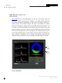
MAIN XFKDISPLAY WINDOW
202
FIGURE 158.
XFXDISPLAY FK PLOT WINDOW
204
FIGURE 159.
GRAPHICAL SECTION OF FK PLOT
205
FIGURE 160.
NUMERICAL OUTPUT OF XFKDISPLAY
207
FIGURE 161.
FUNCTION BUTTONS IN FK PLOT WINDOW
209
FIGURE 162.
MENU AND TOOLBAR OPTIONS IN XFKDISPLAY
210
FIGURE 163.
FILE MENU IN XFKDISPLAY
210
FIGURE 164.
EDIT MENU IN XFKDISPLAY
211
FIGURE 165.
STATION SELECTION WINDOW
212
FIGURE 166.
STATION-SPECIFIC PARAMETER WINDOW
213
FIGURE 167.
RECIPE PARAMETER WINDOW
214
FIGURE 168.
CHANNEL LIST IN XFKDISPLAY WITH ALL CHANNELS SELECTED
216
FIGURE 169.
ARS ALPHALIST BEFORE XFKDISPLAY UPDATE
217
FIGURE 170.
ARS ALPHALIST AFTER XFKDISPLAY UPDATE
217
FIGURE 171.
XFKDISPLAY VIEW MENU
220
FIGURE 172.
ARS AFTER FK BEAM IS RECEIVED FROM XFKDISPLAY
222
FIGURE 173.
FILTER DISPLAY IN XFKDISPLAY
224
Interactive Analysis Subsystem Software User Manual
May 2001
IDC-6.5.1
I D C
D O C U M E N T A T I O N
FIGURE 174.
DEFAULT MAP DISPLAY
226
FIGURE 175.
FILE MENU IN MAP
227
FIGURE 176.
EDIT MENU IN MAP
228
FIGURE 177.
OBJECT DATABASE QUERY OPTIONS
228
FIGURE 178.
EDIT SELECTED OBJECTS OPTIONS IN MAP
229
FIGURE 179.
EDIT LAYERS OPTIONS IN MAP
230
FIGURE 180.
VIEW MENU IN MAP
231
FIGURE 181.
VIEW OBJECTS OPTION IN MAP
232
FIGURE 182.
VIEW SELECTED OBJECTS OPTION IN MAP
232
FIGURE 183.
MAP OUTLINES OPTIONS IN MAP
233
FIGURE 184.
MAP OUTLINES AVAILABLE IN MAP
234
FIGURE 185.
VIEW MAPS OPTIONS IN MAP
235
FIGURE 186.
LIST OF MAP VIEWS AVAILABLE IN MAP
236
FIGURE 187.
ZOOMED IMAGE
238
FIGURE 188.
OVERLAYS AVAILABLE IN MAP
239
FIGURE 189.
MAP DISPLAY OVERLAYS
240
FIGURE 190.
MAP MOUSE POINTER COORDINATES
241
FIGURE 191.
OPTIONS MENU IN MAP
242
FIGURE 192.
MAP ANALYST TOOLS MENU
243
FIGURE 193.
ANOMALOUS EVENT QUALIFIER (AEQ)
245
FIGURE 194.
AEQ ANOMALOUS OUTPUT
245
FIGURE 195.
AEQ MAGNITUDE OUTPUT
246
FIGURE 196.
AEQ LOW SEISMICITY AREAS OUTPUT
246
FIGURE 197.
AEQ DEEP OUTPUT
246
FIGURE 198.
AEQ LOW SEISMICITY AT DEPTH OUTPUT
247
FIGURE 199.
GENERATING DATA REQUEST FROM ARS
249
FIGURE 200.
WAVEEXPERT ASSESS (WEASSESS) TOOL – LIST OF STATIONS
250
FIGURE 201.
WEASSESS COLUMN SORTING OPTIONS
251
FIGURE 202.
BLOCK OF SELECTED STATIONS
253
FIGURE 203.
NON-CONTINUOUS SELECTION OF STATIONS
254
Interactive Analysis Subsystem Software User Manual
IDC-6.5.1
May 2001
I D C
D O C U M E N T A T I O N
FIGURE 204.
MAP SELECTED OPTION IN WEASSESS
255
FIGURE 205.
MAP LAUNCHED FROM WEASSESS
256
FIGURE 206.
USER NAME LEVEL IN IADR STATUS WINDOW
258
FIGURE 207.
IADR (FOLDER LEVELS IN IADR STATUS WINDOW)
259
FIGURE 208.
IADR POP-UP OPTIONS
260
FIGURE 209.
HART
262
FIGURE 210.
HART F-STATISTIC ANNULUS
263
FIGURE 211.
HYDROACOUSTIC PARAMETERS DISPLAY
265
FIGURE 212.
HART WAVEFORM DISPLAY
267
FIGURE 213.
HYDROACOUSTIC AZIMUTH PLOT PARAMETERS
269
FIGURE 214.
COLOR BAR PARAMETERS
270
FIGURE 215.
AZIMUTH MODIFICATIONS BY ANALYST
272
FIGURE 216.
HART FILE MENU
273
FIGURE 217.
POLARIPLOT WINDOW
276
FIGURE 218.
POLARIPLOT PARAMETER DISPLAY
277
FIGURE 219.
POLARIPLOT DEFAULT DISPLAY GRAPHS
278
FIGURE 220.
POLARIPLOT FILE MENU
280
FIGURE 221.
POLARIPLOT DISPLAY/SUBMIT DIALOG BOX
281
FIGURE 222.
EDIT MENU
283
FIGURE 223.
FILTER SUBMENU
283
FIGURE 224.
POLARIPLOT FILTER DIALOGUE BOX
284
FIGURE 225.
ROTATION MODE DIALOGUE BOX
285
FIGURE 226.
SET SUBMENU OPTIONS
286
FIGURE 227.
POLARIPLOT VIEW MENU
287
FIGURE 228.
POLARIPLOT GRAPH DISPLAY OPTIONS
288
FIGURE 229.
VIEW > ZOOM SUBMENU
289
FIGURE 230.
COORDINATES DISPLAY OPTIONS
290
FIGURE 231.
THREE GRID STYLES AVAILABLE FOR DISPLAY IN POLARIPLOT
291
FIGURE 232.
SPECTRAPLOT DISPLAY WITH LINEAR FREQUENCY
292
FIGURE 233.
SPECTRAPLOT FILE MENU
293
Interactive Analysis Subsystem Software User Manual
May 2001
IDC-6.5.1
I D C
D O C U M E N T A T I O N
FIGURE 234.
SPECTRAPLOT EDIT MENU
294
FIGURE 235.
SPECTRAPLOT VIEW MENU
296
FIGURE 236.
SPECTRAPLOT DISPLAY WITH LOG FREQUENCY
298
FIGURE 237.
SPECTRAPLOT DISPLAY OF UNSMOOTHED SPECTRA
300
FIGURE 238.
SPECTRAPLOT DISPLAY OF SMOOTHED SPECTRA
301
FIGURE 239.
DMAN STATUS
WINDOW
303
FIGURE 240.
DMAN STATUS
WINDOW WITH AEQ APPLICATION LAUNCHED
306
FIGURE 241.
DMAN
FIGURE 242.
FLUSHING XFKDISPLAY’S MESSAGE QUEUE
310
FIGURE 243.
EXITING ANALYSIS SESSION
312
FIGURE 244.
ANALYST_LOG
313
FIGURE 245.
ALLOCATION WINDOW
314
FIGURE 246.
ALLOCATION WINDOW DATE AND TIME SECTION
315
FIGURE 247.
UNALLOCATED TIME BLOCK
316
FIGURE 248.
ALLOCATED, ANALYZED, AND SCANNED TIME BLOCK
317
FIGURE 249.
FUNCTIONS IN ANALYST_LOG
317
FIGURE 250.
GRAPHIC ARS BUTTON
322
FIGURE 251.
REBQC
323
FIGURE 252.
MESSAGE OUTPUT FROM ANALYST_LOG
324
FIGURE 253.
QC WINDOW
325
FIGURE 254.
TYPICAL STYLE MANAGER – WINDOW SETTINGS
344
FIGURE 255.
TYPICAL STYLE MANAGER – STARTUP SETTINGS
344
FIGURE 256.
INTERACTIVE ANALYSIS DATABASE ACCESS
352
FIGURE 257.
ANALYST VIEW OF ARS
356
Interactive Analysis Subsystem Software User Manual
IDC-6.5.1
May 2001
MESSAGE QUEUE
CONTROL WINDOW
308
I D C
D O C U M E N T A T I O N
Interactive Analysis Subsystem
Software User Manual
TABLES
TABLE I:
DATA FLOW SYMBOLS
v
TABLE II:
TYPOGRAPHICAL CONVENTIONS
vi
TABLE III:
CONVENTIONS FOR USER INSTRUCTIONS
vi
TABLE 1:
EVENT COLORS
31
TABLE 2:
ARS TOOLBAR FUNCTIONS
41
TABLE 3:
ARS HOT KEY FUNCTIONS
179
TABLE 4:
EVENT FIELDS OF ALPHALIST
182
TABLE 5:
ARRIVAL AREA (MIDDLE AREA) OF ALPHALIST
184
TABLE 6:
CHANNEL AREA OF ALPHALIST
185
TABLE 7:
TOOLBAR FUNCTIONS IN ALPHALIST
186
TABLE 8:
FIELDS IN SOLUTIONS AREA OF LOCATOR BOX
189
TABLE 9:
FUNCTION BUTTONS IN LOCATOR DIALOGUE BOX
191
TABLE 10:
LOCATION ARRIVAL INFORMATION FIELDS
192
TABLE 11:
CURRENT MAGNITUDE (TOP PART) IN MAGNITUDE BOX
196
TABLE 12:
MAGNITUDE DIALOGUE BOX FUNCTIONS
197
TABLE 13:
MAGNITUDE ARRIVALS BOX FIELDS
198
TABLE 14:
XFKDISPLAY FIELDS
202
TABLE 15:
FK PLOT TABULAR OUTPUT
208
TABLE 16:
WEASSESS COLUMN DESCRIPTIONS
250
TABLE 17:
IADR COLUMNS
258
TABLE 18:
HYDRO PARAMS FEATURE
265
TABLE 19:
PLOT PARAMETERS
270
TABLE 20:
COLOR PARAMETERS
271
TABLE 21:
TRACES AVAILABLE IN POLARIPLOT
274
TABLE 22:
POLARIPLOT ACTIVE SERIES FIELDS
277
Interactive Analysis Subsystem Software User Manual
IDC-6.5.1
May 2001
I D C
D O C U M E N T A T I O N
TABLE 23:
FILE MENU FUNCTIONS
293
TABLE 24:
EDIT MENU FUNCTIONS
295
TABLE 25:
VIEW MENU FUNCTIONS
297
TABLE 26:
DMAN
TABLE 27:
OPTIONS MENU
305
TABLE 28:
FEATURES IN TOP SECTION OF ANALYST_LOG
315
TABLE 29:
TIME ALLOCATION SECTION OF ANALYST_LOG
316
TABLE 30:
COTS AND PD SOFTWARE FOR INTERACTIVE ANALYSIS SOFTWARE
339
TABLE 31:
ENVIRONMENT VARIABLES USED BY INTERACTIVE ANALYSIS
SOFTWARE
340
EXAMPLE INTERACTIVE VALIDATION TEST
366
TABLE 32:
COLOR SCHEME
304
Interactive Analysis Subsystem Software User Manual
May 2001
IDC-6.5.1
I D C
D O C U M E N T A T I O N
Te c h n i c a l I n s t r u c t i o n s
About this Document
This chapter describes the organization and content of the document and includes
the following topics:
n
Purpose
n
Scope
n
Audience
n
Related Information
n
Using this Document
Interactive Analysis Subsystem Software User Manual
IDC-6.5.1
May 2001
i
I D C
D O C U M E N T A T I O N
Te c h n i c a l I n s t r u c t i o n s
About this Document
PURPOSE
This document describes how to use the Interactive Analysis Subsystem of the
International Data Centre (IDC). This software is part of the Time-Series Analysis
computer software component (CSC) of the Interactive Processing Computer Software Configuration Item (CSCI).
SCOPE
The manual includes instructions for setting up the software, using its features, and
basic troubleshooting. This document does not describe the software’s design or
requirements. Some of these topics are described in sources cited in “Related Information.”
AUDIENCE
This document is intended for first-time or occasional users of the software. However, more experienced users may find certain sections useful as a reference. The
word “you” in this document refers to an analyst of seismic/hydroacoustic/infrasonic (S/H/I) data.
RELATED INFORMATION
The following documents complement this document:
n
Database Schema [IDC5.1.1Rev2]
n
Configuration of PIDC Databases [IDC5.1.3Rev0.1]
n
IDC Processing of Seismic, Hydroacoustic, and Infrasonic Data [IDC5.2.1]
Interactive Analysis Subsystem Software User Manual
ii
May 2001
IDC-6.5.1
I D C
D O C U M E N T A T I O N
Te c h n i c a l I n s t r u c t i o n s
About this Document
n
Configuration of PIDC Processing Data Files [IDC6.2.4]
n
Distributed Application Control System Software User Manual
▼
[IDC6.5.2Rev0.1]
n
Analyst Review Station Scheme Functions [IDC7.2.2]
See “References” on page 369 for a list of documents that supplement this document. The following UNIX manual (man) pages apply to the existing Time-series
Analysis software:
n
ARS
n
XfkDisplay
n
Map
n
SpectraPlot
n
PolariPlot
n
AEQ
n
IADR
n
HART
n
dman
n
DFX
USING THIS DOCUMENT
This document is part of the overall documentation architecture for the IDC. It is
part of the Technical Instructions category, which provides guidance for installing,
operating, and maintaining the IDC systems. This document is organized as follows:
n
Chapter 1: Introduction
This chapter provides an overview of the software’s capabilities, development, and operating environment.
Interactive Analysis Subsystem Software User Manual
IDC-6.5.1
May 2001
iii
I D C
D O C U M E N T A T I O N
Te c h n i c a l I n s t r u c t i o n s
▼
About this Document
n
Chapter 2: Operational Procedures
This chapter describes how to use the software and includes detailed procedures for startup and shutdown, basic and advanced features, security,
and maintenance.
n
Chapter 3: Troubleshooting
This chapter describes how to identify and correct common problems
related to the software.
n
Chapter 4: Installation and Configuration Procedures
This chapter describes how to install, configure, and validate the software.
n
References
This section lists the sources cited in this document.
n
Glossary
This section defines the terms, abbreviations, and acronyms used in this
document.
n
Index
This section lists topics and features provided in this document along
with page numbers for reference.
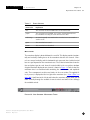
Conventions
This document uses a variety of conventions, which are described in the following
tables. Table I shows the conventions for data flow diagrams. Table II lists typographical conventions. Table III describes the conventions used in instructions for
using the keyboard, commands, and menus.
Interactive Analysis Subsystem Software User Manual
iv
May 2001
IDC-6.5.1
I D C
D O C U M E N T A T I O N
Te c h n i c a l I n s t r u c t i o n s
About this Document
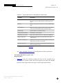
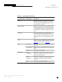
T A B L E I:
▼
D A T A F L OW S YM BOL S
Description
Symbol1
process
#
external source or sink of data
D = disk store
Db = database store
D
control flow
data flow
1. Symbols in this table are based on Gane-Sarson conventions [Gan79].
Interactive Analysis Subsystem Software User Manual
IDC-6.5.1
May 2001
v
I D C
D O C U M E N T A T I O N
Te c h n i c a l I n s t r u c t i o n s
▼
About this Document
T A B L E II:
T Y P O G R A P H I C A L C ON VE N TI ON S
Element
Font
Example
database table
bold
affiliation
database account
CAPS
IDCX:msgdisc
database attributes
italics
mb_ave
processes, software units, and
libraries
analyst_log
user-defined arguments and
variables used in parameter
(par) files or program command lines
<action>.fp
titles of documents
Database Schema
computer code and output
courier
[info]:Parameter inetd - 1
filenames, directories, and
websites
ARS.par
text that should be typed
exactly as shown
ps -fu <cds-user-name>
T A B L E III: C O N V E N T IO N S
FOR
U S E R I N S T RU CTI ON S
Instruction
Explanation
Example
choose
Use keyboard shortcuts or click
once with your (left) mouse
button to select a menu option.
Choose File > Print.
click
Press and release the appropriate mouse button to activate a
graphic object on the screen.
Click Done.
display
A general reference to a window or subsection of a window.
Select one or more channels to
be sorted to the top of the
ARS display.
double-click
Click a mouse button twice
without moving the pointer.
Double-click the icon to
reopen the program.
Interactive Analysis Subsystem Software User Manual
vi
May 2001
IDC-6.5.1
I D C
D O C U M E N T A T I O N
Te c h n i c a l I n s t r u c t i o n s
About this Document
T A B L E III: C O N V E N T I ON S
F OR
U S E R I N S T RU CTI ON S ( CON TI N U E D )
Instruction
Explanation
Example
drag
Hold down the left mouse button while moving the pointer.
Drag the pointer to draw a
rectangle around the region of
interest.
key-key
Indicates simultaneous key
strokes. Hold down the first key
and press the second key.
control-e
Choose (submenu) from
(menu).
File > Print.
press
Press a key or sequence of keys,
or hold down the left mouse
button.
Press the enter key.
pull-down,
pull-up, or
pull-right menu
A list of options related to a
menu. The list appears for as
long as you press on the related
menu.
Choose a year from the Date
pull-down menu.
screen, monitor
Hardware display monitor.
The left screen displays the
Common Desktop Environment (CDE) menu.
select
Highlight or click on data.
Select the text to be copied.
Select a waveform.
toggle
Turn a particular mode on or off
by clicking on a button or key.
Use the Line Style toggle button to switch between grid
modes.
window
Application’s Graphical User
Interface (GUI).
The ARS window includes an
event list.
menu > submenu
▼
(Hold down the control key
and press the letter e.)
(Choose Print from the File
menu.)
Interactive Analysis Subsystem Software User Manual
IDC-6.5.1
May 2001
vii
I D C
D O C U M E N T A T I O N
Te c h n i c a l I n s t r u c t i o n s
Chapter 1: I n t r o d u c t i o n
This chapter provides a general description of the software and includes the following topics:
n
Software Overview
n
Functionality
n
Inventory
n
Environment and States of Operation
Interactive Analysis Subsystem Software User Manual
IDC-6.5.1
May 2001
1
I D C
D O C U M E N T A T I O N
Te c h n i c a l I n s t r u c t i o n s
Chapter 1: I n t r o d u c t i o n
SOFTWARE OVERVIEW
Figure 1 shows the logical organization of the IDC software. The Interactive Analysis Subsystem is part of the Time-series Analysis CSC, which is one component of
the Interactive Processing CSCI. Figure 2 shows the processing flow of the IDC system and the relationship of the Interactive Analysis Subsystem to other components of the system.
The Interactive Analysis Subsystem is comprised of a number of applications that
support interactive analysis of time-series data. The central application for interactive analysis is the Analyst Review Station (ARS), which displays seismic, hydroacoustic, and infrasonic (S/H/I) waveform data and derived parameters. Waveform
data first undergo signal and event analysis during an automated processing
phase. An S/H/I analyst reviews and edits the output of this processing in ARS
(process 3 in Figure 2). The analyst then refines generated arrivals, events, and
location hypotheses and adds new arrivals and events missed during the automated phase. Modifications are saved to an output database. A further stage of
automated processing (process 4 in Figure 2) follows analysis, and the output is
ready for quality review. Lead analysts and other personnel use the interactive
applications during quality review. A bulletin is then published for States’ Parties to
examine.
Besides ARS, a number of associated tools are available for specialized signal analysis and signal feature extraction:
n
XfkDisplay
XfkDisplay is the azimuth and slowness determination tool.
Interactive Analysis Subsystem Software User Manual
2
May 2001
IDC-6.5.1
I D C
D O C U M E N T A T I O N
Chapter 1:
Te c h n i c a l I n s t r u c t i o n s
Introduction
n
▼
Map
Map provides an interactive graphical display of the geographic aspects
of S/H/I data.
IDC Software
Automatic
Processing
Interactive
Processing
Distributed
Processing
Data
Services
Data
Management
System
Monitoring
Data for
Software
Station
Processing
Time-series
Analysis
Application
Services
Continuous
Data
Subsystem
Data
Archiving
System
Monitoring
Automatic
Processing
Data
Network
Processing
Bulletin
Process
Monitoring
and Control
Message
Subsystem
Database
Libraries
Performance
Monitoring
Interactive
Data
Postlocation
Processing
Interactive
Tools
Distributed
Processing
Libraries
Retrieve
Subsystem
Database
Tools
Distributed
Processing
Data
Event
Screening
Analysis
Libraries
Distributed
Processing
Scripts
Subscription
Subsystem
Configuration
Management
Data
Services
Data
Time-series
Tools
Radionuclide
Analysis
Data Services
Utilities and
Libraries
Data
Management
Time-series
Libraries
Web
Subsystem
System
Monitoring
Data
Operational
Scripts
Authentication
Services
COTS
Data
Environmental
Data
Radionuclide
Processing
Atmospheric
Transport
F IG U R E 1.
IDC S OF T W ARE C ON F I G U RAT I ON H I E RARCH Y
Interactive Analysis Subsystem Software User Manual
IDC-6.5.1
May 2001
3
I D C
Chapter 1:
▼
D O C U M E N T A T I O N
Te c h n i c a l I n s t r u c t i o n s
Introduction
n
SpectraPlot
SpectraPlot provides the power spectrum of a waveform segment.
n
Anomalous Event Qualifier (AEQ)
AEQ provides a statistical probability that an event is anomalous, based
on historical data.
n
Interactive Auxiliary Data Request Tool (IADR)
IADR allows the analyst to request additional waveform data from auxil-
iary stations.
n
Hydroacoustic Azimuth Review Tool (HART)
HART allows for interactive analysis of hydroacoustic azimuths.
n
PolariPlot
PolariPlot is a polarization analysis and display tool.
n
Interactive Detection and Feature Extraction (DFX)
DFX calculates features such as amplitude and period from seismic or
hydroacoustic signals.
States
Parties
IMS
IDC
databases
Data import
Data export
1
2
3
4
Station
Processing
Network
Processing
Interactive
Analysis
Post-analysis
Processing
F I G U R E 2.
IDC P R O C E S S IN G F L OW
Interactive Analysis Subsystem Software User Manual
4
May 2001
IDC-6.5.1
I D C
D O C U M E N T A T I O N
Te c h n i c a l I n s t r u c t i o n s
Chapter 1:
Introduction
▼
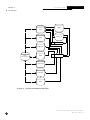
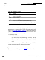
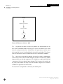
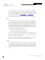
Figure 3 shows a simplified interactive processing flow model. In this model an
analysis session is started through the analyst_log application. In analyst_log, a time
window for analysis is selected and the ARS application is started. The time window parameters are written to the ARS.load data file in the analyst’s home directory. ARS reads the ARS.load file on startup and uses these parameters to
constrain the data it reads and writes to the database. ARS communicates with and
starts the other interactive applications via messages relayed by dman and the
interprocess communication system (IPC). IPC messages specify the permanent
and temporary database tables used for the transfer of data between interactive
applications.
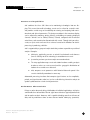
FUNCTIONALITY
The Interactive Analysis Subsystem is designed for analyst review of S/H/I waveform data and automated processing results comprised of events and arrivals. The
central component for analysis is the ARS application. In ARS waveforms are displayed as horizontal time-series traces with arrival times indicated by phase labeled
vertical bars. Event lists are displayed above the waveforms with preliminary estimates of location and origin time. The primary role of ARS and its associated tools
is to allow you to interactively examine arrivals and their attributes as an aid in
determining which arrivals should be associated as an event. ARS and its tools are
also useful for examining and, if necessary, modifying the specific characteristics of
individual arrivals and for defining new arrivals or creating new events where these
were missed by automated processing. ARS interfaces with the database so that
interactive modifications can be saved.
Interactive Analysis Subsystem Software User Manual
IDC-6.5.1
May 2001
5
I D C
Chapter 1:
▼
D O C U M E N T A T I O N
Te c h n i c a l I n s t r u c t i o n s
Introduction
HART
ARS
analyst_log
Map
D
ARS.load
XfkDisplay
dman
IADR
Db
databases
IPC messages
SpectraPlot
PolariPlot
AEQ
F I G U R E 3.
I N T E R A C T I V E P R O CE S S I N G F L OW
Interactive Analysis Subsystem Software User Manual
6
May 2001
IDC-6.5.1
I D C
D O C U M E N T A T I O N
Chapter 1:
Te c h n i c a l I n s t r u c t i o n s
Introduction
▼
Features and Capabilities
ARS combines the three S/H/I time-series monitoring technologies into one dis-
play. This means that multi-technology events can be refined or created in ARS.
ARS provides a wide range of functionality for viewing and analyzing both wave-
form data and derived parameters. The data presentation in the waveform display
can be adjusted by zooming, sorting, filtering, and adding or removing displayed
channels. Arrivals can be added, deleted, retimed, compared with theoretical
arrival times, and associated or disassociated with events. Through ARS you refine,
create, or reject events and save these reviewed events to the database for further
processing in producing a bulletin.
ARS is supported by a group of analysis tools that perform expanded or specialized
analysis. Examples:
n
XfkDisplay graphically presents an arrival’s back-azimuth and slowness
(inverse velocity) to aid in evaluating its association to an event.
n
SpectraPlot performs spectrum analysis on waveform data.
n
The Map application maps event and station locations enabling analysts
to observe where an event occurred and the geographic distribution of
stations where arrivals were detected.
n
AEQ compares event parameters with historical data and reports if the
event is statistically anomalous in some way.
Automated processing functions that compute signal features such as amplitude,
period, and signal-to-noise ratio (snr) can be recalled during interactive analysis to
update hydroacoustic or seismic arrival parameters.
Performance Characteristics
Delays are often observed during initialization of individual applications. ARS takes
considerable time to load data. Four to eight hours of data are typically loaded into
ARS for routine analysis. However, ARS is capable of loading more than 24 hours of
data, and its performance slows as more data are loaded. XfkDisplay, SpectraPlot,
Interactive Analysis Subsystem Software User Manual
IDC-6.5.1
May 2001
7
I D C
Chapter 1:
▼
D O C U M E N T A T I O N
Te c h n i c a l I n s t r u c t i o n s
Introduction
PolariPlot, and AEQ are all initialized when they are first used, but subsequent use
elicits rapid response. Interactive recall processing, IADR, HART, and DFX are initialized each time they are invoked; you will observe some latency with these tools.
ARS is typically used to display waveform data from a large number of stations.
ARS tends to slow briefly when waveform data are manipulated. Larger processing
latencies include aligning arrivals, sorting channels, adding additional channels,
and beaming (although you can select an option for beaming that runs as a background process). Try to analyze one technology at a time. Because the bulk of
events that are built by the automatic system are seismic, seismic data are displayed most of the time. Hydroacoustic waveforms are recorded at a much higher
sampling rate than the other technologies. Infrasonic analysis requires that channels from each recording station at a site be displayed. This can slow the responsiveness of the ARS display. You may wish to display waveforms from these
technologies at the end of an event’s analysis and undisplay them when not in use,
instead of sorting all three technologies together for each event. ARS provides
functions to switch focus from one S/H/I technology to the next.
ARS and its tools are robust. A failure (ARS crash) is not expected with any fre-
quency. A normal rate of failure might be one ARS crash per analyst per week. A
rate higher than this should be investigated if the cause is unknown, especially if a
pattern emerges.
To protect against data loss in the event of a failure, data from your session are
automatically stored in UNIX binary files each time ARS interacts with the database
(save, discard, undiscard, or unfreeze an event). You can also manually save recovery data at your discretion. ARS can be configured to write recovery data either in
your home directory or on your workstation’s local disk to optimize performance.
INVENTORY
This section lists the files, database tables, and database accounts that comprise
the Interactive Analysis Subsystem. The software is one processing component of a
larger S/H/I monitoring system; therefore, these items do not exist in isolation and
are installed as part of the full monitoring system:
Interactive Analysis Subsystem Software User Manual
8
May 2001
IDC-6.5.1
I D C
D O C U M E N T A T I O N
Te c h n i c a l I n s t r u c t i o n s
Chapter 1:
Introduction
▼
Files1
$(CMSS)/X11/Map_xgksfonts/*
$(CMSS)/X11/app-defaults/AEQ
$(CMSS)/X11/app-defaults/ARS
$(CMSS)/X11/app-defaults/Map
$(CMSS)/X11/app-defaults/PolariPlot
$(CMSS)/X11/app-defaults/SpectraPlot
$(CMSS)/X11/app-defaults/XfkDisplay
$(CMSS)/bin/AEQ
$(CMSS)/bin/ARS
$(CMSS)/bin/DFX
$(CMSS)/bin/HART
$(CMSS)/bin/IADR
$(CMSS)/bin/Map
$(CMSS)/bin/PolariPlot
$(CMSS)/bin/SpectraPlot
$(CMSS)/bin/WaveExpert
$(CMSS)/bin/XfkDisplay
$(CMSS)/bin/dman
$(CMSS)/bin/exec_popup
$(CMSS)/bin/start_hart_server
$(CMSS)/bin/tuxshell
$(CMSS)/config/app_config/DFX/*.par
$(CMSS)/config/app_config/DFX/*/*.par
$(CMSS)/config/app_config/DFX/scheme/*.scm
$(CMSS)/config/app_config/distributed/dman/dman.par
$(CMSS)/config/app_config/distributed/tuxshell/interactive/tuxshell<queue>.par
$(CMSS)/config/app_config/interactive/AEQ/AEQ.clp
$(CMSS)/config/app_config/interactive/AEQ/AEQ.par
$(CMSS)/config/app_config/interactive/ARS/ARS.par
$(CMSS)/config/app_config/interactive/ARS/IDC.scm
$(CMSS)/config/app_config/interactive/HART/HART.par
$(CMSS)/config/app_config/interactive/IADR/IADR.par
$(CMSS)/config/app_config/interactive/Map/IDC_MAP.scm
$(CMSS)/config/app_config/interactive/Map/Map_Analyst_Tools.scm
$(CMSS)/config/app_config/interactive/Map/Mapconfig.scm
$(CMSS)/config/app_config/interactive/Map/overlay.scm
$(CMSS)/config/app_config/interactive/XfkDisplay/XfkDisplay.par
$(CMSS)/config/app_config/interactive/XfkDisplay/arrays/*.par
$(CMSS)/config/app_config/interactive/XfkDisplay/recipes/*.par
$(CMSS)/config/app_config/interactive/analyst_log/analyst_log.par
$(CMSS)/config/app_config/interactive/analyst_log/analyst_log.ppm
1. The shorthand notation $(CMSS) is a UNIX environmental parameter that points to the root of the IDC
software directory tree. The * symbol is a wildcard reference to all files or directories in that location.
Interactive Analysis Subsystem Software User Manual
IDC-6.5.1
May 2001
9
I D C
Chapter 1:
▼
D O C U M E N T A T I O N
Te c h n i c a l I n s t r u c t i o n s
Introduction
$(CMSS)/config/earth_specs/BLK_OSO/*
$(CMSS)/config/earth_specs/MAG/atten/atten*
$(CMSS)/config/earth_specs/MAG/atten/slowamp.P
$(CMSS)/config/earth_specs/MAG/mdf/idc_mdf.defs
$(CMSS)/config/earth_specs/MAG/mdf/idc_mdf.defs
$(CMSS)/config/earth_specs/MAG/tlsf/idc_tlsf.defs
$(CMSS)/config/earth_specs/MAG/tlsf/idc_tlsf.defs
$(CMSS)/config/earth_specs/SASC/sasc*
$(CMSS)/config/earth_specs/TT/vmsf/ars.defs
$(CMSS)/config/earth_specs/TT/vmsf/ims.defs
$(CMSS)/config/station_specs/*.par
$(CMSS)/config/system_specs/DFX.par
$(CMSS)/config/system_specs/app-resources/ARS
$(CMSS)/config/system_specs/app-resources/Map
$(CMSS)/config/system_specs/app-resources/SpectraPlot
$(CMSS)/config/system_specs/app-resources/XfkDisplay
$(CMSS)/config/system_specs/automatic.par
$(CMSS)/config/system_specs/env/analyst.dt/*
$(CMSS)/config/system_specs/env/default.*
$(CMSS)/config/system_specs/env/global.env
$(CMSS)/config/system_specs/env/process.dt/icons/*
$(CMSS)/config/system_specs/env/terminfo/*
$(CMSS)/config/system_specs/interactive.par
$(CMSS)/config/system_specs/process.par
$(CMSS)/config/system_specs/shared.par
$(CMSS)/contrib/bin/mon_dd
$(CMSS)/contrib/bin/qcmap
$(CMSS)/jlib/HART.jar
$(CMSS)/jlib/IADR.jar
$(CMSS)/jlib/ipc.jar
$(CMSS)/jlib/libHART_compute.so
$(CMSS)/jlib/libjipc.so
$(CMSS)/jlib/util.jar
$(CMSS)/scheme/ARSdefault.scm
$(CMSS)/scheme/Mapdefault.scm
$(CMSS)/scheme/Mapgc.scm
$(CMSS)/scheme/general.scm
$(CMSS)/scheme/intrinsic.scm
$(CMSS)/scheme/libpar.scm
$(CMSS)/scheme/math.scm
$(CMSS)/scheme/siod.scm
$(CMSS)/scripts/bin/ARSscan
$(CMSS)/scripts/bin/analyst_log
$(CMSS)/scripts/bin/capture_dt.pl
$(CMSS)/scripts/bin/cleanMStables
$(CMSS)/scripts/bin/crInteractive
$(CMSS)/scripts/bin/mkCMSuserq
$(CMSS)/scripts/bin/rebqc
$(CMSS)/scripts/bin/start
Interactive Analysis Subsystem Software User Manual
10
May 2001
IDC-6.5.1
I D C
D O C U M E N T A T I O N
Te c h n i c a l I n s t r u c t i o n s
Chapter 1:
Introduction
▼
$(CMSS)/scripts/bin/today
$(CMSS)config/app_config/automatic/WaveExpert/WaveExpert-IADR-Assess.par
$(CMSS)config/app_config/automatic/WaveExpert/WaveExpert-IADR-Request.par
$(CMSS)config/app_config/automatic/WaveExpert/WaveExpert.par
$(CMSS)config/app_config/automatic/WaveExpert/distance_rule.clp
$(CMSS)config/app_config/automatic/WaveExpert/we_init.clp
$(LOGDIR)/%jdate/interactive/<role>-<host machine>-<pid>
$(LOGDIR)/%jdate/interactive/dman-$(host)-$(USER)-$(agent)
$(LOGDIR)/%jdate/interactive/tuxshell-<role>-<host machine>-<pid>
$(LOGDIR)/HART/<machine>_hart.log
$(LOGDIR)/WaveExpert/<role>.log
$(TUXDIR)/bin/BBL
$(TUXDIR)/bin/TMQFORWARD
$(TUXDIR)/bin/TMQUEUE
$(TUXDIR)/bin/TMS/TMS_QM
$(TUXDIR)/bin/TMSYSEVT
$(TUXDIR)/bin/TMUSREVT
$(TUXDIR)/bin/tmboot
$(TUXDIR)/bin/tmshutdown
$(TUXDIR)/config/scripts/templates/ubb.analysis_template
/var/tuxedo/PIDC70_analysis/TLOGS/tlog
/var/tuxedo/PIDC70_analysis/ULOGS/ULOG<jday>
/var/tuxedo/PIDC70_analysis/config/tuxconfig
/var/tuxedo/PIDC70_analysis/config/ubb
~/.ARSinit
~/.Mapinit
~/.Xdefaults
~/.cshrc
~/.dt/*
~/.login
~/ARS.history
~/ARS.load
Interactive Analysis Subsystem Software User Manual
IDC-6.5.1
May 2001
11
I D C
Chapter 1:
▼
D O C U M E N T A T I O N
Te c h n i c a l I n s t r u c t i o n s
Introduction
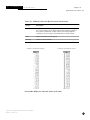
D a t a b a s e Ta b l e s
affiliation
allocate_hour
amp3c
ampdescript
amplitude
apma
arrival
assoc
colordisc
detection
discard
dseisgrid
dseisindex
event
event_control
hydro_arr_group
hydro_assoc
hydro_features
instrument
interval
lastid
mapcolor
mapdisc
mapover
mappoint
msgdisc
na_value
netmag
origerr
origin
overlaydisc
parrival
remark
request
seisgrid
seisindex
sensor
site
siteaux
sitechan
stamag
timestamp
wfdisc
wftag
Database Accounts
STATIC
SEL3
IDCX
LEB
MAP
Interactive Analysis Subsystem Software User Manual
12
May 2001
IDC-6.5.1
I D C
D O C U M E N T A T I O N
Te c h n i c a l I n s t r u c t i o n s
Chapter 1:
Introduction
▼
Te m p o r a r y D a t a b a s e Ta b l e s
ims$_ARS_wfdisc_<tmp id>
ims$_ARS_arrival_<tmp id>
ims$_ARS_amplitude_<tmp id>
ims$_ARS_apma_<tmp id>
ims$_ARS_in_origin_<tmp id>
ims$_ARS_out_origin_<tmp id>
ims$_ARS_in_origerr_<tmp id>
ims$_ARS_out_origerr_<tmp id>
ims$_ARS_in_assoc_<tmp id>
ims$_ARS_out_assoc_<tmp id>
ims$_ARS_arrival_<tmp id>
ims$_ARS_amplitude_<tmp id>
ims$_ARS_apma_<tmp id>
ims$_ARS_amp3c_<tmp id>
ims$_ARS_detection_<tmp id>
ims$_ARS_wfdisc_<tmp id>
ims$_ARS_wftag_<tmp id>
ims$_ARS_assoc_<tmp id>
ims$_ARS_hydro_features_<tmp id>
ims$_ARS_arrival_<tmp id>
ims$_ARS_assoc_<tmp id>
ims$_ARS_origin_<tmp id>
ims$_ARS_origerr_<tmp id>
ims$_ARS_wftag_<tmp id>
Interactive Analysis Subsystem Software User Manual
IDC-6.5.1
May 2001
13
I D C
Chapter 1:
▼
D O C U M E N T A T I O N
Te c h n i c a l I n s t r u c t i o n s
Introduction
ENVIRONMENT AND STATES OF
OPERATION
Software Environment
The software is configured to run under Solaris 7 (Sun Microsystem’s version of
UNIX), CDE 1.3.2, and X11R6.4 and Motif 2.1 windowing libraries. The software
depends on the ORACLE 8i database server and the Tuxedo version 6.5 interprocess communication software.
Hardware Environment
You must select the hardware on which to run the software components. Software
components are generally mapped to hardware to be roughly consistent with the
software configuration model. A typical analyst workstation is a Sun Microsystems
Ultra60 computer with dual CPU, 512 megabytes of Random Access Memory
(RAM) and dual Creator 3D 24-bit color graphics boards driving dual 21” display
monitors. Less powerful hardware configurations of Sun Microsystem’s workstations will run the software, but with degraded performance.
Normal Operational State
The Interactive Analysis Subsystem components are used interactively by operators
trained in the analysis of S/H/I technology sources. Analysis sessions are initiated
by analyst action using a custom configured Sun CDE windowing interface. Individual modules are launched in response to interprocess communication actions
using the Tuxedo interprocess communication libraries and initialized using
ORACLE database tables, configuration parameter files, and X window resource
configuration files. Post interactive analysis recall processing is initiated via database triggers configured into the ORACLE database and activated by analyst
actions in the analyst_log application.
Interactive Analysis Subsystem Software User Manual
14
May 2001
IDC-6.5.1
I D C
D O C U M E N T A T I O N
Te c h n i c a l I n s t r u c t i o n s
Chapter 1:
Introduction
▼
Contingencies/Alternate States of
Operation
The software requires a trained operator and is not intended for use in automated
or offline mode. In normal operation the software takes its input from the Standard
Event List 3 (SEL3) and saves its output to the Late Event Bulletin (LEB) ORACLE
database accounts. ARS and its associated tools can be configured to run using
database accounts other than these (for example, for training or research purposes). Individual applications can be launched from the UNIX command line if
proper command line parameters are provided. UNIX manual (man) pages for each
application are available to document command line usage.
Interactive Analysis Subsystem Software User Manual
IDC-6.5.1
May 2001
15
I D C
D O C U M E N T A T I O N
Te c h n i c a l I n s t r u c t i o n s
Chapter 2: O p e r a t i o n a l
Procedures
This chapter provides instructions for using the software and includes the following
topics:
n
Software Startup
n
Software Shutdown
n
Basic Procedures
n
Analyst Review Station (ARS) Procedures
n
XfkDisplay Procedures
n
Map Procedures
n
Anomalous Event Qualifier (AEQ) Procedures
n
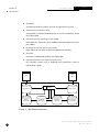
Interactive Auxiliary Data Request (IADR) Procedures
n
Hydroacoustic Azimuth Review Tool (HART) Procedures
n
PolariPlot Procedures
n
SpectraPlot Procedures
n
dman Procedures
n
analyst_log Procedures
n
Advanced Procedures
n
Maintenance
n
Security
Interactive Analysis Subsystem Software User Manual
IDC-6.5.1
May 2001
17
I D C
D O C U M E N T A T I O N
Te c h n i c a l I n s t r u c t i o n s
Chapter 2: O p e r a t i o n a l
Procedures
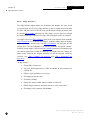
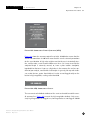
SOFTWARE STARTUP
The Interactive Analysis Subsystem is comprised of a number of programs for
interactive analysis of time-series data. The central component of the software is
ARS, which displays S/H/I waveform data. Additional tools are provided to per-
form specialized analysis. In general, no single application is launched to run independently of the others, and when used in conjunction the components provide
complete information about an arrival or an event. In normal usage, analysis is performed in the main ARS display. When you require more specific detail about an
arrival, groups of arrivals, or an event, ARS sends messages to specific tools to handle the specialized analysis. In response to these messages, the tool is launched to
immediately receive and respond to the message and return results to ARS as
required.
Typically an analysis session begins with analyst_log. You use the analyst_log application to allocate a time period for analysis, to specify the appropriate data for
loading into ARS, to launch ARS, and to trigger certain post-analysis processes.
Detailed procedures for analyst_log, ARS, and the other applications are provided
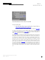
in subsequent sections. The UNIX operating system automatically displays the CDE
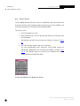
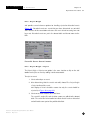
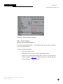
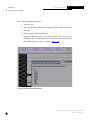
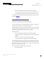
menu bar when you log onto your workstation. To conveniently launch analyst_log
(and start the analysis session) the CDE menu bar at the bottom of the screen has
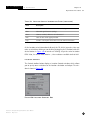
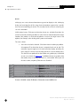
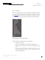
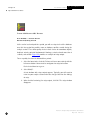
been customized to include the Start Analyst Review menu button as shown in Figure 4.
Interactive Analysis Subsystem Software User Manual
18
May 2001
IDC-6.5.1
I D C
D O C U M E N T A T I O N
Chapter 2:
Te c h n i c a l I n s t r u c t i o n s
Operational Procedures
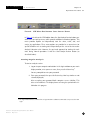
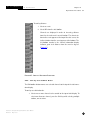
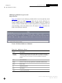
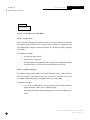
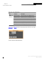
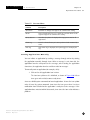
F IG U R E 4.
▼
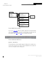
CDE M E N U B AR S H OW I N G S T ART A N AL YS T R E VI E W
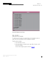
In Figure 4, the tab on the CDE toolbar above the Start Analyst Review button provides access to a pull-up menu, which provides additional customized options. This
menu provides options to independently start the dman, HART, ARS, and
analyst_log applications. These menu options are provided as a convenience for
special situations such as starting ARS independently of the rest of the Interactive
Analysis Subsystem suite. However, the preferred approach for starting the software during normal operations is with the Start Analyst Review button (as
described below).
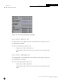
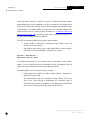
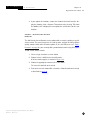
Starting Regular Analysis
To start an analysis session:
1. Log on to your computer workstation. In the login window on your main
display monitor, enter your user name, then press the Return key.1
You are prompted to enter your password.
2. Enter your password, then press the Return key. Your key strokes are not
echoed (displayed).
After accepting your password both computer screens initialize. This
takes a few moments. The display shows an hour glass symbol while initialization is in progress.
1. The login window offers a command line or login window in addition to CDE. Make sure you use the CDE
login.
Interactive Analysis Subsystem Software User Manual
IDC-6.5.1
May 2001
19
I D C
Chapter 2:
▼
D O C U M E N T A T I O N
Te c h n i c a l I n s t r u c t i o n s
Operational Procedures
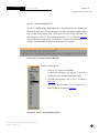
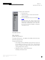
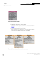
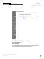
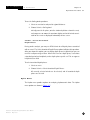
3. After initialization, the CDE toolbar is located at the bottom
of both display screens. The fourth icon button from the
left is the Start Analyst Review button shown here. Click
this button to start analyst_log.
The analyst_log application is displayed on your right screen.
4. In analyst_log (and referring to the “analyst_log Procedures” on
page 312) choose the Allocation option, and select a time period for
analysis. Next, run the ARSscan option to update the ARS.load file.
5. When this process is complete, click the large ARS graphic
(shown here) at the bottom middle of the Allocation window in analyst_log.
Three programs are initiated. The dman and ARS programs
are launched, and their application windows appear on the left screen.
WEAssess is also initiated (see “Interactive Auxiliary Data Request (IADR)
Procedures” on page 248).
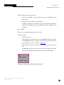
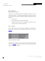
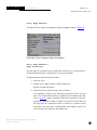
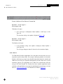
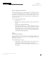
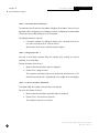
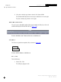
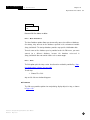
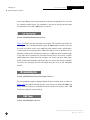
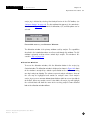
An ARS window appears with only the toolbar and menu displayed. No
waveform data are displayed upon initial launch. The initial ARS window
is shown in Figure 5.
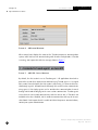
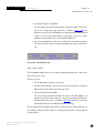
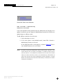
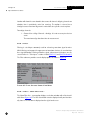
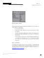
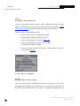
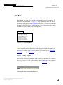
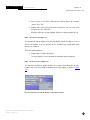
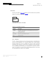
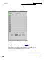
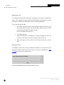
6. To load data, choose File > Read.
The date and time that were selected in analyst_log appear in a dialogue
box, as shown in Figure 6. The operational database and network are
also specified.
7. After checking the information, click Done in the dialogue box.
ARS begins the process of loading the waveform data for that time
period, along with automatically processed arrivals and events.
You can now begin processing the data, using the procedures described in the subsequent sections.
Interactive Analysis Subsystem Software User Manual
20
May 2001
IDC-6.5.1
I D C
D O C U M E N T A T I O N
Chapter 2:
Te c h n i c a l I n s t r u c t i o n s
Operational Procedures
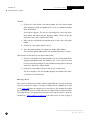
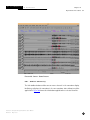
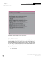
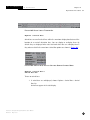
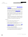
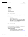
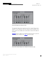
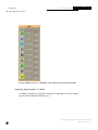
F IG U R E 5.
ARS M AI N W I N D OW
AT
▼
S TART U P
Startup Notes
Loading data into ARS can take several minutes. The waveform display partially
refreshes during the load process. After the display is complete and the hour-glass
cursor has been replaced by a pointer cursor you can begin interacting with the
data. In the initial waveform display ARS shows the entire loaded time window,
normally four hours. At this time scale, waveforms are shown only as straight lines
where data are present. You will need to zoom in to see actual waveforms.
Interactive Analysis Subsystem Software User Manual
IDC-6.5.1
May 2001
21
I D C
Chapter 2:
▼
D O C U M E N T A T I O N
Te c h n i c a l I n s t r u c t i o n s
Operational Procedures
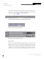
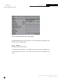
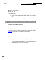
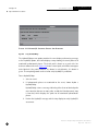
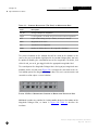
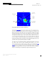
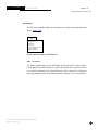
F I G U R E 6.
ARS
READ
W IN DOW
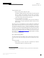
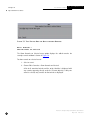
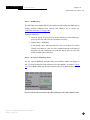
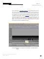
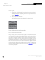
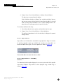
When started, ARS displays the status of the Tuxedo interprocess communication
system, which ARS uses for communicating with the other analysis tools. If Tuxedo
is running, ARS reports this with the message shown in Figure 7.
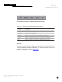
F I G U R E 7.
ARS IPC S T A T U S M E S S AG E
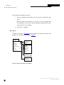
By default, the first session is run as Tuxedo agent 1. All applications launched as
part of this session then communicate with ARS using Tuxedo agent 1. If a second
ARS session is launched while the first session is still running, it is connected to Tux-
edo through agent 2. All tools launched through this second session communicate
using agent 2. Put simply, agents can be considered as communication channels
through which tools belonging to the same session communicate. Tuxedo agents
ensure that the correct tool communicates with the correct ARS. If Tuxedo is not
available or has been disabled, ARS is unable to communicate with any of its associated tools. If ARS reports that it is unable to initiate interprocess communications,
contact your system administrator.
Interactive Analysis Subsystem Software User Manual
22
May 2001
IDC-6.5.1
I D C
D O C U M E N T A T I O N
Te c h n i c a l I n s t r u c t i o n s
Chapter 2:
Operational Procedures
▼
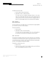
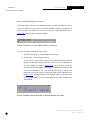
SOFTWARE SHUTDOWN
You normally exit an analysis session either by choosing File > Exit in ARS or by
using the Kill All option in dman.
To exit ARS through the File menu:
1. In ARS, choose File > Exit.
A confirmation dialogue box appears. If unsaved changes exist in the
ARS session, the dialogue box indicates that changes will be discarded.
2. To continue to exit, click OK.
To exit ARS and all tools related to the ARS agent from dman:
1. Select Kill All in dman.
dman presents a confirmation dialogue box.
2. Click OK to send an exit signal to all running applications using the same
Tuxedo agent.
The tools exit without presenting additional dialogue box prompts.
Exit all Interactive Analysis Subsystem applications before you use the EXIT button
on the CDE tool bar to log out of your UNIX session.
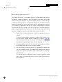
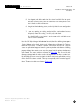
BASIC PROCEDURES
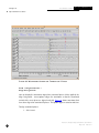
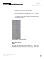
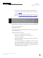
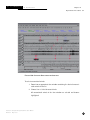
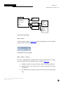
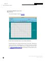
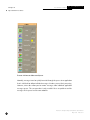
Session Display Organization
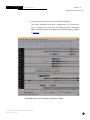
The typical analyst workstation uses two screens to display ARS and its associated
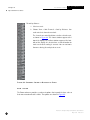
tools. Generally, the ARS session is displayed on the left screen (0.0 screen), while
the other tools are displayed on the right screen (0.1 screen). The left screen
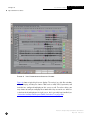
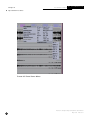
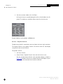
shown in Figure 8 contains the CDE toolbar at the bottom, the ARS main window,
and the dman window. You may also display and use a mail tool, text editor, or
interactive shell window during an analysis session. Examples of these are shown in
Figure 8, iconified or in a closed-window state.
Interactive Analysis Subsystem Software User Manual
IDC-6.5.1
May 2001
23
I D C
Chapter 2:
▼
D O C U M E N T A T I O N
Te c h n i c a l I n s t r u c t i o n s
Operational Procedures
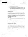
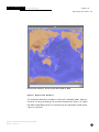
F I G U R E 8.
LEFT SCREEN
DURING
A N AL YS I S S E S S I ON
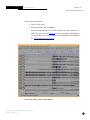
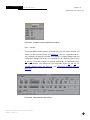
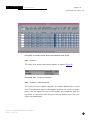
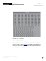
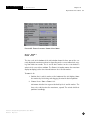
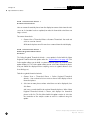
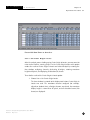
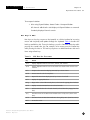
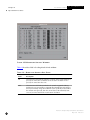
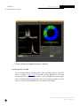
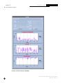
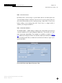
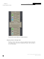
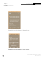
Figure 9 shows a typical right screen display. The analyst_log, ARS filter window,
AEQ, XfkDisplay, and Map are shown. Tools such as IADR, HART, SpectraPlot, and
PolariPlot are configured to display on this screen as well. To reduce clutter, you
may choose to iconify or undisplay these tools while they are not in use. WEAssess
is also launched to display on the right screen, but is generally kept iconified (see
“Interactive Auxiliary Data Request (IADR) Procedures” on page 248).
Interactive Analysis Subsystem Software User Manual
24
May 2001
IDC-6.5.1
I D C
D O C U M E N T A T I O N
Chapter 2:
Te c h n i c a l I n s t r u c t i o n s
Operational Procedures
▼
Figures 8 and 9 show the default display configuration. You may prefer a different
display for your analysis session. “Chapter 4: Installation and Configuration Procedures” on page 337 provides further information about changing this configuration.
F IG U R E 9.
R IG H T S CRE E N
D U RI N G
A N AL YS I S S E S S I ON
Interactive Analysis Subsystem Software User Manual
IDC-6.5.1
May 2001
25
I D C
Chapter 2:
▼
D O C U M E N T A T I O N
Te c h n i c a l I n s t r u c t i o n s
Operational Procedures
Using Menus
ARS and the other applications each contain a menu bar across the top of their
window. This menu bar contains one or more pull-down menus. A pull-down (or
pull-up, pull-right) menu expands to show a list of options related to the menu.
There are two methods to open a main menu. For the first method, click once on
the menu name with the left mouse button to reveal the menu and submenu
options. Then click the left mouse button on the menu or submenu option to select
it. The options remain open. For the second method, click on the main menu, and
drag the mouse to the desired option or submenu, then release the button. The
submenus are highlighted and open one by one when you drag the mouse over
them. Using this method, the menu options close on release. The click-dragrelease method can be used however deeply the submenus are nested. To select
the desired menu option, drag the mouse through the submenus until the desired
option is highlighted, then release the mouse. This activates the function.
In addition to menus, ARS and several other applications provide toolbars with
labeled buttons, which provide quick access to commonly used functions. To activate a function from the toolbar, click on the toolbar button once using your left
mouse button.
Using Common Mouse Actions
Several mouse button actions are commonly used in the Interactive Analysis Subsystem applications. Often you will need to select an object such as an arrival or
channel in ARS or a station location in Map. To select an object, position the mouse
pointer over the object, and click on the object once using your left mouse button.
When objects are selected they become highlighted.
Another common action is double-clicking. This involves clicking the left mouse
button twice in quick succession without moving the pointer. For example, the ARS
Filter Selection window presents a list of filter options. Double-clicking a filter
option both selects and applies the filter in one operation.
Interactive Analysis Subsystem Software User Manual
26
May 2001
IDC-6.5.1
I D C
D O C U M E N T A T I O N
Chapter 2:
Te c h n i c a l I n s t r u c t i o n s
Operational Procedures
▼
A drag action requires that you press the left mouse button while moving the
pointer (a click-drag-release operation). Drag actions were used in the previous
section to select submenu items in one step. Another example is to use the drag
action to move an object, such as in manually resizing a display window. This is
done by moving the cursor to the corner of the window, clicking on the corner
object, and dragging the corner to a new location, making the window larger or
smaller. Release the mouse when the desired size is set.
Often the data presented in a display are too large to fit completely in the available
window size. Scroll bars allow you to control which portion of the data to display in
the window. Scroll bars are vertical/horizontal depending on the nature of the displayed data. To scroll, click or drag in various portions of the scroll bar.
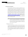
Scheme and Shell Windows
A number of applications provide a Scheme or shell window in addition to their
graphical window. These are text windows that display additional status and error
messages. They start in an iconified or minimized state to take up as little screen
area as possible. You can double-click on them to open them. Those applications
that provide a Scheme interface, notably ARS and Map, are able to interpret
Scheme commands in the shell window. An introduction to ARS Scheme is provided
in [IDC7.2.2].
Obtaining Help
In addition to the IDC documentation listed in “References” on page 369, man
pages provide useful sources for additional information on the applications. Man
pages are available for ARS, AEQ, analyst_log, dman, HART, IADR, Map, PolariPlot,
SpectraPlot, and XfkDisplay. Often a Help button is provided in an application’s
menu bar; this button usually provides a brief description for functions within that
window.
When you hover the cursor over a menu option or toolbar button in ARS, a quicktip appears. Quick-tips provide more complete function names than are provided
in the cryptic menu or button label (see “Quick-tips” on page 37).
Interactive Analysis Subsystem Software User Manual
IDC-6.5.1
May 2001
27
I D C
Chapter 2:
▼
D O C U M E N T A T I O N
Te c h n i c a l I n s t r u c t i o n s
Operational Procedures
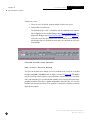
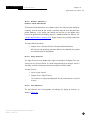
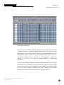
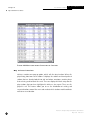
ANALYST REVIEW STATION (ARS)
PROCEDURES
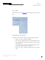
ARS Window Layout and
Organization
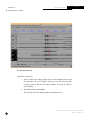
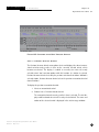
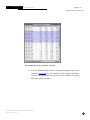
The main ARS window is the central focus for time-series analysis. Within its borders events are reviewed or built, and access to the majority of the Interactive
Analysis Subsystem’s functionality is provided. The ARS main window shown in
Figure 10 is a busy display, rich in information.
F I G U R E 10. M A IN ARS W IN DOW
Interactive Analysis Subsystem Software User Manual
28
May 2001
IDC-6.5.1
I D C
D O C U M E N T A T I O N
Chapter 2:
Te c h n i c a l I n s t r u c t i o n s
Operational Procedures
▼
This window displays the following items:
n
Functions
n
Events
n
Waveforms
n
Waveform Labels
n
Amplitude Scaling and Measurement
n
Deselecting All Objects
n
Time Bar
n
Message Area
n
Resizing Areas in the ARS Window
n
Quick-tips
n
Popup Menus
Functions
The top section of the ARS main window contains pull-down menus and toolbar
buttons, as shown in Figure 11. A Help function at the top right provides a limited
description of the available functionality. The toolbar buttons provide shortcuts to
functions commonly used during an analysis session. Each menu option and button
is described individually in “Toolbar Button Functions” on page 41 and “ARS
Menus” on page 68.
F IG U R E 11. ARS M E N U S
AN D
T OOL BAR B U TTON S
Interactive Analysis Subsystem Software User Manual
IDC-6.5.1
May 2001
29
I D C
Chapter 2:
▼
D O C U M E N T A T I O N
Te c h n i c a l I n s t r u c t i o n s
Operational Procedures
Events
The event scrolling list is located below the ARS toolbar (Figure 12). The list displays all events built by the Automatic Processing software and any events that
you create during analysis. Each event is identified by the event identification number (evid), the time of the event, and the latitude/longitude of the event.
F I G U R E 12. ARS E V E N T L IS T
Quick-tips on the event objects (see “Quick-tips” on page 37) display the origin
identification number (orid). The terms event and origin are often used synonymously, even in ARS menus. Generally, analysts refine events to determine the
most accurate origin. In the course of event refinement, several different origins
may be computed. This document will use the term event to refer to the objects
that analysts work with and will use the term origin to refer to the result of an
event’s location computation.
To select an event, click the square box beside the event. To select additional
events, press the shift key while clicking the additional events. If you select an
event without pressing the shift key, all other events are unselected. To view additional events, use the scroll bar below the list to scroll left or right through all
events in the time window.
Events are labeled in different colors, depending on their status. Table 1 explains
the color scheme.
Interactive Analysis Subsystem Software User Manual
30
May 2001
IDC-6.5.1
I D C
D O C U M E N T A T I O N
Chapter 2:
Te c h n i c a l I n s t r u c t i o n s
Operational Procedures
T A B L E 1:
▼
E V E N T C OL ORS
Event Color
Explanation
blue
The event has not been modified since it was last located.
purple
The event has been modified; one or more associated arrivals have
been modified. Locating the event will return it to blue.
red/orange
An arrival originally associated to this event has been reassociated to
another event.
green
The event has been saved.
brown
The event has been discarded.
Wa v e f o r m s
The waveform display is located below the event list. This display contains horizontally and vertically scrolling traces of the waveform data for each channel. Channels are arrayed vertically, and the horizontal axis represents time. Labeled arrival
bars are superimposed on the waveform traces. These labeled arrival bars show the
time and phase type for each channel’s arrivals visible in the current time window.
A typical waveform display for one channel is shown in Figure 13. To the left of the
waveform trace is a waveform label containing the channel name and amplitude
scale. These components are discussed further in the next section. The applied filter, if present, is displayed at the far right of the waveform (see “View > Filter” on
page 106). Scroll bars to the left of and below the waveform display allow you to
move vertically through the available channels or back and forth in time through
the available arrivals.
F IG U R E 13. O N E C H AN N E L W AVE F ORM T RACE
Interactive Analysis Subsystem Software User Manual
IDC-6.5.1
May 2001
31
I D C
Chapter 2:
▼
D O C U M E N T A T I O N
Te c h n i c a l I n s t r u c t i o n s
Operational Procedures
ARS was designed to display waveforms from all three time-series technologies,
seismic, hydroacoustic, and infrasonic, to allow for an integrated analysis of each
event. The travel times for signal energy differ depending on technology (that is,
on the medium through which it propagates), with seismic waves traveling the
fastest, hydroacoustic waves traveling somewhat slower, and infrasonic waves
traveling considerably slower still. In addition to the waveform time window, which
you initially specified, ARS loads an additional 20 minutes of seismic data, an additional 1.5 hours of hydroacoustic data, and an additional 5 hours of infrasonic
data. This additional data allows the energy from events occurring near the end of
the time window to reach more distant stations and still be viewable in the ARS
waveform display.
Wa v e f o r m L a b e l s
Waveform labels are displayed to the left of their associated waveforms. A number
of different channel types may be displayed: vertical components, horizontal components, or beamed channels. The name of the channel is the combination of the
abbreviation of the station name and the abbreviation of the channel component.
For example, in Figure 13 the channel name is MJAR/cb representing the coherent
beam channel at station MJAR (Matsushiro, Japan).
The great-circle distance from the station to the event location (in degrees) is displayed beneath the channel name. The station-to-event azimuth (in degrees) from
north is displayed to the right, separated by a slash.
Amplitude Scaling and
Measurement
A waveform amplitude scale bar is located between the waveform trace and the
channel name. This bar looks like a capital letter E. Waveforms are displayed as
demeaned digital instrument counts. By default the waveform is auto-scaled so
that the maximum amplitude within the display window fits into the channel’s
available display area. The two numbers at the top and bottom of the scale bar are
the waveform vertical scale and the waveform offset. By clicking and dragging the
middle mouse button over the waveform vertical scale (top number), the wave-
Interactive Analysis Subsystem Software User Manual
32
May 2001
IDC-6.5.1
I D C
D O C U M E N T A T I O N
Chapter 2:
Te c h n i c a l I n s t r u c t i o n s
Operational Procedures
▼
form’s height is scaled larger or smaller. Waveform data are clipped if they extend
outside the channel’s display area. Figures 14 and 15 show example waveforms
before and after height adjustment.
F IG U R E 14. W A V E F ORM
BE F ORE
F IG U R E 15. W A V E F ORM
AF T E R
H E I G H T A D JU S TM E N T
H E I G H T A D JU S TM E N T
By clicking the middle mouse button over the bottom number, the scaling jumps
by a factor of 10. This adjustment is often too coarse for practical use. Click and
move the right mouse button over the scale bar to adjust the waveform offset; this
method moves the waveform up and down in the waveform display without
changing its amplitude scaling, as shown in Figure 16. Scrolling or zooming resets
to auto-scaling.
F IG U R E 16. W A V E F ORM
AF T E R
O F F S E T A D JU S TM E N T
Using mouse actions within the waveform trace you can display demeaned waveform counts or obtain a calibrated measure of period and amplitude. Right click
where desired in the waveform display to show the time and relative amplitude at
Interactive Analysis Subsystem Software User Manual
IDC-6.5.1
May 2001
33
I D C
Chapter 2:
▼
D O C U M E N T A T I O N
Te c h n i c a l I n s t r u c t i o n s
Operational Procedures
that time as shown in Figure 17. Because amplitude counts are demeaned and possibly filtered, they appear as positive or negative floating point numbers (for example, the –0.8 value shown in Figure 17).
F I G U R E 17. V I E W S E L E C T E D T I M E
AN D
A M P L I TU D E C OU N TS
Period and amplitude are measured based on a selected arrival.
To measure the period and amplitude:
1. Select an arrival by left clicking on the arrival label. The arrival label is surrounded with an open box when the cursor is in the selection area and
with a closed box when selected.
2. Using the right mouse button, select a maximum or minimum within a
few seconds after the selected arrival time.
Time and counts are displayed, as shown in Figure 17.
3. Using the right mouse button, select a maximum or minimum on the
waveform one full period later.
The half-period and calibrated amplitude (in nanometers) is computed
and displayed, as shown in Figure 18.
F I G U R E 18. V I E W P E R IO D /2
AN D
C ORRE S P ON D I N G A M PL I T U D E
Interactive Analysis Subsystem Software User Manual
34
May 2001
IDC-6.5.1
I D C
D O C U M E N T A T I O N
Chapter 2:
Te c h n i c a l I n s t r u c t i o n s
Operational Procedures
▼
Deselecting All Objects
You can deselect all channels and arrivals by clicking once with the left mouse button anywhere in the waveform display except on a channel name or phase label;
that is, click any place in the waveform display that will not select an object. This
action deselects all currently selected channels and arrivals in the waveform display.
Selected events remain selected.
Time Bar
The time bar is located beneath the horizontal scroll bar for the waveform display,
as shown in Figure 19. This part of the ARS window presents the time scale for the
currently displayed waveforms and varies depending on the originally loaded time
window, the current zoom level, and the position of the horizontal scroll bar. The
time scale units are displayed at the bottom of the time bar. Time scaling is delineated in units of 1/10 seconds, seconds, minutes, hours, or days. The date and
time of the left edge of the viewed time window is displayed at the bottom left of
the time bar.
F IG U R E 19. T IM E B AR
IN
ARS
Two dynamic time scale markers labeled t1 and t2 are displayed on the time scale.
Each marker is labeled with its current offset on the time scale. The absolute time
difference between the two markers, labeled |t2-t1|, is displayed at the bottom of
the time bar. Use mouse drag actions to move the markers horizontally on the time
scale. Use t1 when adjusting an existing arrival’s time or to mark a time to add a
new arrival (see “Edit > Retime” on page 82 and “Edit > Add Arrival…” on
page 86). Use t1 and t2 to mark a subset of the current display for zooming in or
magnifying the waveform view.
Interactive Analysis Subsystem Software User Manual
IDC-6.5.1
May 2001
35
I D C
Chapter 2:
▼
D O C U M E N T A T I O N
Te c h n i c a l I n s t r u c t i o n s
Operational Procedures
To zoom:
1. Click on the t1 bar with the left mouse button. Press the mouse button
while dragging it along the bottom of the screen in a horizontal motion
to the desired time.
A vertical line appears. This line runs up through the entire ARS waveform display and moves with the dragging motion. This line helps you
track where the t1 bar is relative to the data.
2. When you are satisfied with the position of the t1 bar, release the mouse
button.
3. Perform the same actions with the t2 bar.
4. Select the zoom function (use control-z or choose Edit > Zoom).
The waveform display zooms to the time window defined by t1 and t2.
To determine the time difference between two arrivals:
1. Click the t1 bar with the left mouse button. Press the mouse button while
dragging horizontally along the bottom of the screen until the vertical
line that extends up through the ARS window overlaps with the desired
arrival time. Release the mouse button.
2. Perform the same action with the t2 bar for the second arrival.
The |t2–t1| output in the time window displays the absolute time difference between the two arrivals.
Message Area
When ARS has performed an action requiring explanation or if an error or warning
must be issued to the analyst, a message is displayed at the bottom of the ARS
screen. Figure 20 shows an example of such a message. In this example the analyst
has attempted to retime an arrival more than 4 seconds from its original location.
This action breaks a rule programmed into ARS so an error message is sent to the
window (see “Edit > Retime” on page 82 in the Edit menu). As each message is
Interactive Analysis Subsystem Software User Manual
36
May 2001
IDC-6.5.1
I D C
D O C U M E N T A T I O N
Chapter 2:
Te c h n i c a l I n s t r u c t i o n s
Operational Procedures
▼
sent to the window, ARS scrolls the message area to display the most recent message. A small scroll bar to the left of the message area allows you to see previous
messages.
F IG U R E 20. M E S S AG E A RE A
IN
ARS
An alarm bell indicator is located at the right of the message area. By
default ARS launches with the alarm bell turned on. The bell sounds
when ARS reports a message. To turn the bell off, select it using the
left mouse button. A line will appear drawn through the bell indicating that the sound has been turned off.
Resizing Areas in the ARS
Window
In the complete ARS window shown in Figure 10 on page 28, the menu and toolbar, event list, waveform/time bar, and message areas are separated by horizontal
lines with a square tab toward their right ends. You can resize these areas within
the ARS window by using the left mouse button to drag the tabs up or down.
Dragging the line above the message area allows you to view more error messages, but sacrifices the size of the waveform area in the process.
Quick-tips
Other interactive features of the ARS window are quick-tips and popup menus.
This section describes quick-tips; popup menus are described in the next section.
Quick-tips are descriptions of ARS functions and objects, which appear when you
hover the cursor over a function or object. If you place the cursor over a toolbar
button or menu option (but not a submenu name) a one-line description of the
Interactive Analysis Subsystem Software User Manual
IDC-6.5.1
May 2001
37
I D C
Chapter 2:
▼
D O C U M E N T A T I O N
Te c h n i c a l I n s t r u c t i o n s
Operational Procedures
menu option or tool bar button’s function appears. If you place the cursor over a
channel, event, or arrival object, additional information about these objects
appears. Figures 21 through 23 show examples of quick-tips.
F I G U R E 21. Q U IC K - T I P D E S CRI BI N G T OOL B AR A L P H F U N CTI ON
F I G U R E 22. Q U IC K - T I P D I S P L AYI N G
ORI D
F I G U R E 23. Q U IC K - T I P D I S P L AYI N G
ARI D
Popup Menus
Popup menus also provide additional information about event, channel, or arrival
objects, and provide easy access to functions specific to the object. By rightclicking on the event, channel, or arrival, you are provided with a list of menu
items that you can select directly from the popup menu. For example, if you select
a popup menu on a channel, functions commonly applied to channels such as fil-
Interactive Analysis Subsystem Software User Manual
38
May 2001
IDC-6.5.1
I D C
D O C U M E N T A T I O N
Te c h n i c a l I n s t r u c t i o n s
Chapter 2:
Operational Procedures
▼
tering or zooming appear. If you select a popup menu for an event, you can access
information about each arrival associated to the event without having to search for
them. Figures 24 through 26 show example popup menus.
F IG U R E 24. C H A N N E L P OP U P M E N U
Interactive Analysis Subsystem Software User Manual
IDC-6.5.1
May 2001
39
I D C
Chapter 2:
▼
D O C U M E N T A T I O N
Te c h n i c a l I n s t r u c t i o n s
Operational Procedures
F I G U R E 25. E V E N T P O P U P M E N U
Interactive Analysis Subsystem Software User Manual
40
May 2001
IDC-6.5.1
I D C
D O C U M E N T A T I O N
Chapter 2:
Te c h n i c a l I n s t r u c t i o n s
Operational Procedures
▼
F IG U R E 26. A R R IVAL P OP U P M E N U
To o l b a r B u t t o n F u n c t i o n s
For accessibility, frequently used menu functions are provided on the ARS toolbar,
as shown in Figure 27. These functions modify the waveform display, modify arrivals, or call associated tools. Toolbar buttons are displayed directly above the waveform display. Table 2 provides a list of the toolbar options. A detailed description of
the functions follows Table 2.
F IG U R E 27. ARS T OOL BAR
T A B L E 2:
ARS T OOL BAR F U N CTI ON S
Tool
Description
Asc On
select associated phases
Co Ph
disassociate coda phases
Uftr
unfilter channel(s)
Interactive Analysis Subsystem Software User Manual
IDC-6.5.1
May 2001
41
I D C
Chapter 2:
▼
D O C U M E N T A T I O N
Te c h n i c a l I n s t r u c t i o n s
Operational Procedures
T A B L E 2:
ARS T O O L B A R F U N CT I ON S ( CON T I N U E D )
Tool
Description
Ph “P”
default phase
Ad Ph
add phase
Rn Ph
rename phase
Bm Ph
beam phase
AlPh
align on default phase
UnAl
unalign phase
SBD
sort by distance
SBU
sort by user-defined order
Th
display theoretical arrival time
Th O
undisplay theoretical arrivals
F-K
analyze azimuth and slowness using XfkDisplay
Beam
beam channel(s)
SlCh
select channel
Ele
select element
Loc
locate event
Rej
reject event
QC
perform quality check
Ufrz
unfreeze event
Sav
save event
Asc On - Select Associated
Phases
The Asc On toolbar button selects all phases associated with the single selected
event.
Interactive Analysis Subsystem Software User Manual
42
May 2001
IDC-6.5.1
I D C
D O C U M E N T A T I O N
Te c h n i c a l I n s t r u c t i o n s
Chapter 2:
Operational Procedures
▼
To select associated phases:
1. Select a single event.
2. Select AscOn from the ARS toolbar.
All arrivals associated to the event are selected in the ARS waveform display. These can be seen in Figure 28 as having their phase label displayed
in reverse video. The arrivals are also selected in AlphaList if it is displayed
(see “Edit > AlphaList” on page 95).
F IG U R E 28. S E L E C T A S S OCI ATE D P H AS E S
Interactive Analysis Subsystem Software User Manual
IDC-6.5.1
May 2001
43
I D C
Chapter 2:
▼
D O C U M E N T A T I O N
Te c h n i c a l I n s t r u c t i o n s
Operational Procedures
Co Ph - Disassociate Coda Phases
The Co Ph toolbar button disassociates coda phases. Coda phases are generally
defined as those arrivals, whether associated or not, that appear closely in time
behind a main arrival and that have similar azimuth and slowness to the main
arrival’s phase type. These arrivals trigger the detector, but are not likely to be a
distinct phase; they are reverberations following the appearance of the main phase
and are not assigned travel times; they are assigned the suffix x, such as Px or tx,
to distinguish them as coda to main phases. Although coda arrivals are often associated to an event by the Automatic Processing software, you may want to disassociate them to remove clutter from the display and AlphaList. Figure 29 shows an
example where only coda phases are selected.
To disassociate a coda phase:
1. Select an event. (Be certain that no other arrivals are selected prior to
selecting Co Ph or they will also be disassociated from the event.)
2. Select Co Ph from the ARS toolbar.
All associated coda phases are added to the selection list, and then all
selected arrivals are disassociated.
Interactive Analysis Subsystem Software User Manual
44
May 2001
IDC-6.5.1
I D C
D O C U M E N T A T I O N
Te c h n i c a l I n s t r u c t i o n s
Chapter 2:
Operational Procedures
▼
F IG U R E 29. S E L E C T C OD A P H AS E S
U f t r - U n fi l t e r C h a n n e l ( s )
The Uftr toolbar button unfilters one or more channels in the waveform display.
Unfiltering redisplays the waveform in its raw waveform state without any filter
applied to it. Figure 30 shows the Uftr button applied to three selected channels.
Interactive Analysis Subsystem Software User Manual
IDC-6.5.1
May 2001
45
I D C
Chapter 2:
▼
D O C U M E N T A T I O N
Te c h n i c a l I n s t r u c t i o n s
Operational Procedures
F I G U R E 30. U N F I L T E R
To unfilter a channel(s):
1. Select a channel by clicking directly in the channel display to the left of
the waveform. To select multiple channels, press the shift key while
selecting channels with the left mouse button. To select all channels,
press control-p.
2. Select Uftr from the ARS toolbar.
The selected channel(s) display unfiltered waveform traces.
Interactive Analysis Subsystem Software User Manual
46
May 2001
IDC-6.5.1
I D C
D O C U M E N T A T I O N
Chapter 2:
Te c h n i c a l I n s t r u c t i o n s
Operational Procedures
▼
Ph “P” - Set Default Phase
The Ph “P” toolbar button both displays the current default phase and allows you
to set the default phase. The default phase is used by several other toolbar buttons
such as add phase (Ad Ph) and rename phase (Rn Ph). When ARS starts, the
default phase is set to “P” so the button is labeled Ph “P”, as shown in Figure 31.
The default phase is also reset to “P” whenever events are saved or discarded. The
button’s label will update whenever the default phase is changed.
F IG U R E 31. S E T D EF AU L T P H AS E B U T T ON
To set the default phase:
1. Select Ph “P” from the ARS toolbar.
A select phase dialogue box appears. It presents a
scrolling list of the available S/H/I phase types.
2. Select the desired phase such as “PcP,” as shown in
Figure 32.
The default phase becomes “PcP,” and the Ph “P”
label is updated, as shown in Figure 33.
F IG U R E 32. S E L E C T P H AS E D I AL OG U E B OX
Interactive Analysis Subsystem Software User Manual
IDC-6.5.1
May 2001
47
I D C
Chapter 2:
▼
D O C U M E N T A T I O N
Te c h n i c a l I n s t r u c t i o n s
Operational Procedures
F I G U R E 33. S E T D E F A U L T P H AS E B U T T ON S H OW I N G P H AS E “P C P”
Ad Ph – Add Phase
The Ad Ph toolbar button adds a default phase to the selected channel’s waveform
at the time marked by t1. The added arrivals are assigned the default phase type
and a negative arrival identifier as shown in Figure 34. Arrivals must be added one
at a time.
F I G U R E 34. A N A L Y S T - A D D E D P H AS E
To add a phase:
1. Position t1 at the desired arrival time.
2. Select a channel.
Interactive Analysis Subsystem Software User Manual
48
May 2001
IDC-6.5.1
I D C
D O C U M E N T A T I O N
Te c h n i c a l I n s t r u c t i o n s
Chapter 2:
Operational Procedures
▼
3. Select Ad Ph from the ARS toolbar.
An arrival is added to the selected channel and is given the default phase
type. If an event is selected the arrival is automatically associated to the
event.
Rn Ph – Rename Phase
The Rn Ph toolbar button renames a phase to the default phase, as shown in Figure 35.
F IG U R E 35. R E N A M E D P H AS E
To rename a phase:
1. Select one arrival; you need not select an event.
2. Select Rn Ph from the ARS toolbar.
The phase name changes to match the default phase name as shown on
the default phase button. If a single event is selected the phase automatically is associated to the event.
Interactive Analysis Subsystem Software User Manual
IDC-6.5.1
May 2001
49
I D C
Chapter 2:
▼
D O C U M E N T A T I O N
Te c h n i c a l I n s t r u c t i o n s
Operational Procedures
Bm Ph – Beam Phase
Beamforming enhances coherent signals relative to background noise. Signal
energy arriving at individual elements of an array is time-shifted and summed to
emphasize energy arriving at the array from a particular direction, such as a theoretical event location. “Beaming” is performed by the DFX application [IDC7.1.1].
The Bm Ph button initiates interactive recall processing to have DFX form beamed
data for the selected station around the selected arrival time oriented toward the
selected event.
To create a beam for a selected phase type:
1. Select an event.
2. Select the fkb or cb beam channel of an array station.
3. Select an arrival to set the phase and time for beaming. You can select
channels for more than one station to generate multiple beams.
4. Select Bm Ph from the ARS toolbar.
A temporary, derived origin beam channel is created. The beam waveform spans several seconds before and after the selected arrival’s theoretical arrival time, based on the origin time and location. Beaming by
DFX takes several seconds, and no dialogue box is displayed while the
beam is being processed. ARS is still active while beamforming occurs.
When the beam is returned, the channels in ARS re-sort to accommodate
the beam. They are sorted by distance to the event. Figure 36 shows a
temporary beam channel for station CMAR.
Interactive Analysis Subsystem Software User Manual
50
May 2001
IDC-6.5.1
I D C
D O C U M E N T A T I O N
Te c h n i c a l I n s t r u c t i o n s
Chapter 2:
Operational Procedures
▼
F IG U R E 36. T E M P O RARY B E AM C H AN N E L
AlPh – Align on Default Phase
The AlPh toolbar button aligns waveforms on the default phase’s theoretical arrival
time as determined by the event’s current location and origin time, and the theoretical travel time from the event to the station.
To align waveforms on the default phase:
1. Select an event.
2. Set the default phase if necessary.
3. Select AlPh from the ARS toolbar.
All waveforms are time shifted to align to the default phase’s theoretical
arrival time at each station.
Interactive Analysis Subsystem Software User Manual
IDC-6.5.1
May 2001
51
I D C
Chapter 2:
▼
D O C U M E N T A T I O N
Te c h n i c a l I n s t r u c t i o n s
Operational Procedures
UnAl – Unalign Phase
The UnAl toolbar button unaligns waveforms. This function removes any time
shifting of the waveforms and displays all channels on the same relative time axis.
To unalign a phase:
1. Select UnAl from the ARS toolbar.
The waveforms in ARS realign to absolute time. They no longer are
aligned on any theoretical travel time or origin time.
SBD – Sort by Distance
The SBD toolbar button sorts channels by distance from the event based on the
event’s current location.
Interactive Analysis Subsystem Software User Manual
52
May 2001
IDC-6.5.1
I D C
D O C U M E N T A T I O N
Chapter 2:
Te c h n i c a l I n s t r u c t i o n s
Operational Procedures
▼
To sort by distance:
1. Select an event.
2. Select SBD from the ARS toolbar.
Channels are displayed in order of increasing distance
from the selected event’s current location. The closest station to the event appears at the top of the ARS screen; the
furthest station from the event appears at the bottom. The
left bottom number in the channel information display
indicates great circle distance from the event in degrees
(Figure 37).
F IG U R E 37. S O R T
BY
D I S TAN CE F U N CT I ON
S B U – S o r t b y U s e r - d e fi n e d O r d e r
The SBU toolbar button moves user-selected channels to the top of the ARS waveform display.
To sort by user-defined order:
1. Select one or more channels to be sorted to the top of ARS display. To
select more than one channel, press the Shift key while selecting multiple
stations, one at a time.
Interactive Analysis Subsystem Software User Manual
IDC-6.5.1
May 2001
53
I D C
Chapter 2:
▼
D O C U M E N T A T I O N
Te c h n i c a l I n s t r u c t i o n s
Operational Procedures
2. Select SBU from the ARS toolbar.
All selected channels are shown at the top of the ARS display, as shown
in Figure 38.
F I G U R E 38. S O R T
BY
U S E R - DE F I N E D O RD E R
Th – Theoretical Arrival Time
The Th toolbar button displays the selected phase’s theoretical arrival time. The
theoreticals displayed are based on the event’s current location and origin time and
on standard travel time curves for the phase.
To display the theoretical arrival time:
1. Select an event.
2. Select channel(s) on which theoretical phases should be displayed.
3. Select Th from the ARS toolbar.
A list of phases is displayed.
Interactive Analysis Subsystem Software User Manual
54
May 2001
IDC-6.5.1
I D C
D O C U M E N T A T I O N
Chapter 2:
Te c h n i c a l I n s t r u c t i o n s
Operational Procedures
▼
4. Select one phase for which theoreticals should be displayed.
The arrival’s theoretical arrival time is displayed on the selected channel(s). If waveforms are aligned on the theoretical phase, theoreticals
appear vertically aligned in the middle of the waveform display, as shown
in Figure 39.
F IG U R E 39. D I S P L A YI N G T H E ORE T I CAL A RRI VAL T I M E S
Interactive Analysis Subsystem Software User Manual
IDC-6.5.1
May 2001
55
I D C
Chapter 2:
▼
D O C U M E N T A T I O N
Te c h n i c a l I n s t r u c t i o n s
Operational Procedures
Th O – Theoretical Times Off
The Th O toolbar button removes theoretical arrival times to avoid clutter. After
selecting a new event or updating an event location, displayed theoreticals are no
longer current and should be removed.
To remove theoretical arrival times:
1. Select Th O from the ARS toolbar. Channels do not have to be selected.
All theoretical phases are removed from the ARS display.
F-K – Analyze Azimuth and
Slowness using XfkDisplay
The F-K toolbar button launches XfkDisplay. This program allows you to visually
interpret the station-to-event azimuth and slowness for an arrival.
To analyze azimuth and slowness using XfkDisplay:
1. Select an arrival. To select more than one arrival to send to XfkDisplay,
press the Shift key while selecting the arrivals one at a time.
2. Select F-K from the ARS toolbar.
XfkDisplay launches, and you can now analyze the arrival’s azimuth and
slowness. You can also return updated azimuth and slowness parameters
to ARS. See “XfkDisplay Procedures” on page 201.
Beam – Beam Channel
Beamforming enhances coherent signals relative to background noise. Signal
energy arriving at individual elements of an array is time-shifted and summed to
emphasize energy arriving at the array from a particular direction, such as a theoretical event location. “Beaming” is performed by the DFX application [IDC7.1.1].
The Beam toolbar button initiates interactive recall processing to have DFX form
beamed data for the selected station around the selected theoretical arrival time
oriented toward the selected event. The Beam function behaves the same as the
function Bm Ph (Beam Phase), except it allows interactive phase selection and
brings up a cancellable dialogue box during processing.
Interactive Analysis Subsystem Software User Manual
56
May 2001
IDC-6.5.1
I D C
D O C U M E N T A T I O N
Te c h n i c a l I n s t r u c t i o n s
Chapter 2:
Operational Procedures
▼
To beam a channel:
1. Select an event.
2. Select either the fk beam or cb beam on an array station (a cb derived
channel is always returned). You can select channels for more than one
station to generate multiple beams.
3. Select Beam from the ARS toolbar.
A list of phases appears.
4. Select the phase on which to beam.
This determines the theoretical arrival time around which the beam interval is created. An ARS dialogue box appears during beam processing,
locking the ARS screen. Beaming should take approximately 15 seconds,
after which time the ARS screen is released, and the appropriate beam
appears. The beam is sorted by distance from the event and aligned on
the theoretical arrival time of the selected phase.
SlCh – Select Channel
ARS displays a default set of channels for each station. The SICh toolbar button
allows you to select additional channel components for display in ARS, as shown in
Figure 40.
F IG U R E 40. C H A N N E L C OM P ON E N TS S E L E CT I ON B OX
Interactive Analysis Subsystem Software User Manual
IDC-6.5.1
May 2001
57
I D C
Chapter 2:
▼
D O C U M E N T A T I O N
Te c h n i c a l I n s t r u c t i o n s
Operational Procedures
To select a channel:
1. Select any channel in a station.
2. Select SlCh from the ARS toolbar.
A list of the station’s components is displayed, as shown in Figure 40.
3. Select a channel type from the list of components, then click Done.
ARS displays all traces belonging to the selected channel type. The chan-
nel(s) appear, sorted by distance from the event, usually along with the
other components of that station. They appear as unfiltered traces, but
are aligned on the default phase. These added channels remain displayed
for the duration of the ARS session or until you remove them manually
(see “ View > Remove Channels” on page 113).
Ele – Element
The Ele toolbar button allows you to select and display individual elements of a
station.
To select an element:
1. Select a channel.
2. Select Ele from the ARS toolbar.
3. Select a channel from the list of elements, as shown in Figure 41, then
click Done.
ARS displays the element. The channel is sorted by distance to the event,
usually along with the other elements of the selected station’s channels.
It appears as an unfiltered trace, but is aligned on the default phase.
Interactive Analysis Subsystem Software User Manual
58
May 2001
IDC-6.5.1
I D C
D O C U M E N T A T I O N
Te c h n i c a l I n s t r u c t i o n s
Chapter 2:
Operational Procedures
▼
F IG U R E 41. C H A N N E L S E L E CTI ON D I AL OG U E B OX
Loc – Locate
The Locate toolbar button computes a location using the arrival time, azimuth, and
slowness of the associated arrivals (see [IDC5.2.1]). ARS uses a grid-point convergence algorithm to compute a location, then displays a Location dialogue box and
a Magnitude dialogue box on the screen opposite the one displaying ARS (Figures
42 and 43). These boxes contain the location information, the computed surface
and depth solutions, and station and event magnitude (Figures 44 and 45) (see
“Locator Dialogue Box” on page 187 and “Magnitude Dialogue Box” on
page 194).
F IG U R E 42. L O C A TOR D I AL OG U E B OX
Interactive Analysis Subsystem Software User Manual
IDC-6.5.1
May 2001
59
I D C
Chapter 2:
▼
D O C U M E N T A T I O N
Te c h n i c a l I n s t r u c t i o n s
Operational Procedures
F I G U R E 43. A S S O C IA T E D A R RI VAL S D I AL OG U E B OX
Interactive Analysis Subsystem Software User Manual
60
May 2001
IDC-6.5.1
I D C
D O C U M E N T A T I O N
Te c h n i c a l I n s t r u c t i o n s
Chapter 2:
Operational Procedures
▼
F IG U R E 44. M A G NI TU D E D I AL OG U E B OX
Interactive Analysis Subsystem Software User Manual
IDC-6.5.1
May 2001
61
I D C
Chapter 2:
▼
D O C U M E N T A T I O N
Te c h n i c a l I n s t r u c t i o n s
Operational Procedures
F I G U R E 45. M A G N IT U D E A R RI VAL S D I AL OG U E B OX
To locate an event:
1. Select an event.
2. Select Locate from the ARS toolbar. Arrivals or channels need not be
selected.
ARS locates the event. The location is displayed in the Locator dialogue
box. The event information in AlphaList (see page 95) and the event
scroll bar at the top of the ARS screen are also updated. Arrival information in AlphaList is updated. Theoretical arrival times are adjusted.
Interactive Analysis Subsystem Software User Manual
62
May 2001
IDC-6.5.1
I D C
D O C U M E N T A T I O N
Te c h n i c a l I n s t r u c t i o n s
Chapter 2:
Operational Procedures
▼
The Locator dialogue box (Figure 42) contains locations for three possible depth
solutions: S = Surface, F = Free, and R = Fixed. The latitude and longitude of the
event, the time of the event, the calculated depth, the number of defining phases,
the location standard error and error ellipse information, and standard error on the
depth are displayed in the Locator dialogue box. The number of iterations required
to converge on a location is also displayed. Several functions can be accessed
through the Locator dialogue box, including the Arrivals option, which displays
detailed information about the arrivals contributing to the location, and a Controls
option, which provides additional options to constrain the location. More information about the Locator dialogue box is provided on page 187.
The Magnitude dialogue box (Figure 44) provides output from the mb_ave and
ml_ppn event or netmag calculation. (The term netmag is short for network magnitude and is used to describe the magnitude of an event, using all the associated
arrival stamags in the network. The term stamag is short for individual station
magnitude. A stamag is calculated from the period and amplitude information
measured from each individual associated arrival that contributes to the magnitude
calculation.) The Magnitude dialogue box displays the magnitude for each calculated depth solution and highlights the preferred depth solution. The preferred
solution is selected automatically as the one producing the smallest error ellipse.
You may change the preferred solution by selecting the small square Pref, which is
next to the preferred solution in the Locator dialogue box (Figure 42). ARS calculates both an mb_ave and ml_ppn. The mb_ave is the averaged bodywave magnitude, calculated for stations between 20 and 100 degrees distance from an event.
The ml_ppn is the averaged local magnitude calculated for stations less than 20
degrees from events that are less than 40 km deep. The magnitude, standard error,
and number of defining phases are displayed in the Magnitude dialogue box for
both types of magnitudes (Figure 44). Like the Locator dialogue box, the Magnitude dialogue box provides several options, including the Arrivals option to display
more detailed information about the individual phases contributing to the event
magnitude (Figure 45). See “Magnitude Dialogue Box” on page 194 for more
information.
Interactive Analysis Subsystem Software User Manual
IDC-6.5.1
May 2001
63
I D C
Chapter 2:
▼
D O C U M E N T A T I O N
Te c h n i c a l I n s t r u c t i o n s
Operational Procedures
Rej – Reject Event
The Rej toolbar button discards or rejects an automated, system-generated event
that you determine to be improperly defined. Rejecting an event invalidates it so
that it does not appear in the Reviewed Event Bulletin (REB).
To reject an event:
1. Select and analyze an event.
2. After determining the event is not valid, discard it by selecting Rej from
the ARS toolbar.
ARS prompts you with a list of reasons for rejection, as shown in Figure
46.
3. Select one or more discard reason, then click Done.
The event identification (evid), analyst ID, and rejection reasons are
added to the discard table. The event label turns brown, as shown in Figure 47. This indicates that the event has been discarded and will not
become part of the published bulletin.
F I G U R E 46. R E A S O N S
FOR
R E JE CT I N G E VE N T
Interactive Analysis Subsystem Software User Manual
64
May 2001
IDC-6.5.1
I D C
D O C U M E N T A T I O N
Chapter 2:
Te c h n i c a l I n s t r u c t i o n s
Operational Procedures
▼
F IG U R E 47. R E J E C T E D E VE N T
QC – Quality Check
The QC toolbar button performs a quality check on events. These checks notify
you of timing and residual errors, improper associations, invalid phase names,
improper defining parameters, errors on depth phase associations, and other less
common errors. Normally you will want to wait until completing your analysis of
an event before invoking QC.
To QC an event:
1. Select QC from the ARS toolbar.
The screen becomes locked while the quality check is run.
When the quality check is complete, a popup text window appears on
top of the ARS window. This popup window provides the results of the
quality check, as shown in Figure 48. Events must meet a minimum number of weighting criteria to be published in the REB. The criteria are
defined in [IDC5.2.1]. Criteria are translated into points in ARS. For
example, a time defining phase is assigned 1 point. The QC output indicates whether an event has sufficient points to be properly saved to the
database for inclusion in the REB. The QC output flags most errors,
including residual errors, improper defining parameters, and so forth. You
must fix these errors before saving the event. The QC provides warnings
only; it does not prevent ARS from saving the event.
Interactive Analysis Subsystem Software User Manual
IDC-6.5.1
May 2001
65
I D C
Chapter 2:
▼
D O C U M E N T A T I O N
Te c h n i c a l I n s t r u c t i o n s
Operational Procedures
F I G U R E 48. E X A M P L E
OF
QC O U T P U T
F ROM
E VE N T
Ufrz – Unfreeze event
Occasionally you may change your opinion of an event. Additional data may
become available after you have saved an event, or you may want to reverse a
previous decision or make a questionable phase non-defining. You cannot change
an event that is in the frozen or saved state; you must first unfreeze the event to
make changes. The Ufrz toolbar button unfreezes an event.
To unfreeze a saved event:
1. Select the event.
Interactive Analysis Subsystem Software User Manual
66
May 2001
IDC-6.5.1
I D C
D O C U M E N T A T I O N
Chapter 2:
Te c h n i c a l I n s t r u c t i o n s
Operational Procedures
▼
2. Select Ufrz from the ARS toolbar.
The event label and associated arrival bars and phase labels, which were
green in the saved state, now turn blue, as shown in Figure 49. Event
parameters saved in the LEB database are removed and are only retained
in ARS. (If ARS is terminated without re-saving the event, the event’s
attributes revert to those set in the input SEL3 database.)
3. You can now modify the event. Save or discard the event after reanalysis;
all events must be in either a saved or discarded state at the end of analysis.
F IG U R E 49. U N F R OZ E N E VE N T
Sav – Save event
The Sav toolbar button saves an event. After completing analysis on a valid event,
you must save the event.
To save an event:
1. Select and perform analysis on an event.
2. Perform a final location, and run QC on the event to make sure that it
adheres to the rules defined for saving an event.
3. Select Sav from the ARS toolbar.
The event and its associated arrivals are saved in the LEB database. To
indicate the saved or frozen state, the event label, associated arrival bars,
and phase labels turn green, as shown in Figure 50. Neither the event nor
associated arrivals can be modified without unfreezing.
An event appears in the REB only if it has been saved in ARS. If you do not save an
event before exiting the ARS session, any changes made to the event during that
session are lost.
Interactive Analysis Subsystem Software User Manual
IDC-6.5.1
May 2001
67
I D C
Chapter 2:
▼
D O C U M E N T A T I O N
Te c h n i c a l I n s t r u c t i o n s
Operational Procedures
F I G U R E 50. S A V E D E V E N T
ARS Menus
The ARS menus are organized by function. Related functions are grouped.
File Menu
The File menu lists functions that read, write, or affect data saved in the database.
The ARS File menu is shown in Figure 51.
File
Read…
Read Recovery Data…
Write Recovery Data
Save Event
Unfreeze
Reject Origin
Exit…
Unfreeze Origins
Unfreeze Arrivals
Reject
UnReject
Show Reason
F I G U R E 51. F IL E M E N U
File > Read…
The Read menu option is usually the first option that you choose in an ARS session.
Read displays a dialogue box through which you can specify the date and time, the
duration, the network, and the database account of the data to be read.
Interactive Analysis Subsystem Software User Manual
68
May 2001
IDC-6.5.1
I D C
D O C U M E N T A T I O N
Chapter 2:
Te c h n i c a l I n s t r u c t i o n s
Operational Procedures
▼
To specify data to be read:
1. With a new ARS session, choose File > Read.
ARS displays a dialogue box with the date and time interval of requested
data, the network, and the database from which data is to be loaded.
The suggested values are taken from the file ARS.load, which is located
in your home directory and generated by analyst_log.
2. Verify the information, then click Done.
The waveform data, event information, arrivals, and channel display are
loaded into ARS. This process typically takes about 5 minutes for a time
block of 4 hours.
When data are first read ARS displays the full time window. Each technology has
display window limits beyond which the waveforms will display as flat line traces.
These limits are 30 minutes for seismic, 1.5 hours for hydroacoustic, and 5 hours
for infrasonic. If the time interval being loaded into ARS is greater than these limits,
you will need to zoom in to a smaller time window to view actual waveforms. The
arrivals bars will be displayed at larger time windows, but may have their phase
labels omitted. The “Options Menu” on page 129 provides options for showing
and unshowing these display items.
File > Read Recovery Data…
The Read Recovery Data menu option recovers changes that you have made, if
you lose your ARS session either through system failure or abnormal ARS termination.
To read recovery data:
1. Upon starting a new ARS session after an abnormal exit,1 instead of
selecting Read, choose File > Read Recovery Data.
1. Use dman to restart ARS instead of the ARS button in analyst_log, which will unsuccessfully attempt to
start another dman.
Interactive Analysis Subsystem Software User Manual
IDC-6.5.1
May 2001
69
I D C
Chapter 2:
▼
D O C U M E N T A T I O N
Te c h n i c a l I n s t r u c t i o n s
Operational Procedures
2. Follow the same procedures as with the Read option.
You are presented with a popup window containing the information that
you requested.
3. Review the data in the popup window, then click Done.
ARS loads the data that you were working on before the crash.
The previous session is returned with any changes you made to arrivals,
parameter measurements such as DFX and XfkDisplay results, and
updated event locations. The status of the events is preserved as either
saved or discarded. However, the ARS functional state is not preserved
from the previous session. Such things as zoom level, selected objects,
and applied filters are not retained. Only updates to event and arrival
characteristics are preserved.
F i l e > Wr i t e R e c o v e r y D a t a
The Write Recovery Data menu option directs ARS to save the current session into
a UNIX binary file. The binary file is read using the Read Recovery Data option.
ARS automatically saves recovery data during database access operations. These
operations include saving, rejecting, unfreezing, or undiscarding an event. This
option allows you to manually save recovery data at your discretion (for example,
when working on a large event). You should not have to use this feature routinely,
because it is regularly invoked automatically.
To write recovery data:
1. Choose File > Write Recovery at any point during analysis to save the
current session updates.
The recovery data are saved.
File > Save Event
The Save Event menu option saves an analyzed event to the database. In an operational setting, saved events are published in the REB.
Interactive Analysis Subsystem Software User Manual
70
May 2001
IDC-6.5.1
I D C
D O C U M E N T A T I O N
Chapter 2:
Te c h n i c a l I n s t r u c t i o n s
Operational Procedures
▼
To save an event:
1. Select and perform analysis on an event.
2. Complete analysis, perform a final location, and QC the event.
3. Choose File > Save Event.
Event data are saved, and the event becomes frozen.
The event appears in the REB only if you have saved it in ARS. If you do not save
the event and you exit the ARS session, any changes you made to the event are
lost.
File > Unfreeze
The Unfreeze menu option provides two submenu options: Unfreeze Origins and
Unfreeze Arrivals, as shown in Figure 52. These options allow you to unfreeze an
origin or arrival(s) and make modifications.
F IG U R E 52. U N F R E E Z E S U BM E N U
File > Unfreeze >
Unfreeze Origins
The Unfreeze Origins menu option is the same as Ufrz in the ARS toolbar.
Occasionally, you may change your opinion of an event. Sometimes additional
data become available after you have saved an event, or you may want to make a
questionable phase non-defining. You cannot make changes to an event that has
Interactive Analysis Subsystem Software User Manual
IDC-6.5.1
May 2001
71
I D C
Chapter 2:
▼
D O C U M E N T A T I O N
Te c h n i c a l I n s t r u c t i o n s
Operational Procedures
been saved; you must first unfreeze the event. The Unfreeze Origins menu option
unfreezes an event and its associated arrivals. Only after the event is unfrozen can
you make changes, relocate, and save the event.
To unfreeze origins:
1. Select the saved event that you want to modify.
2. Choose File > Unfreeze > Unfreeze Origins.
The event, which was labeled green while it was in the saved state, now
turns blue. All of the arrivals also become unfrozen and turn blue. The
event is now ready for modifications.
3. Modify the event as necessary.
4. Save or discard the event after reanalysis. All SEL3 (Standard Event List)
events should be either in a saved or discarded state at the end of your
analysis session, or the changes will be lost.
File > Unfreeze >
Unfreeze Arrivals
The Unfreeze Arrivals menu option allows you to unfreeze specific arrivals. You can
only unfreeze an arrival if it is not associated to an event. If an arrival is associated
to an event that is saved, you must unfreeze the entire event.
To unfreeze arrivals:
1. Select the unassociated, saved arrival.
2. Choose File > Unfreeze > Unfreeze Arrivals.
The individual arrival turns blue and can now be modified. If the arrival is
associated to a saved event, ARS provides a warning that you must first
unfreeze the entire event.
Interactive Analysis Subsystem Software User Manual
72
May 2001
IDC-6.5.1
I D C
D O C U M E N T A T I O N
Te c h n i c a l I n s t r u c t i o n s
Chapter 2:
Operational Procedures
▼
File > Reject Origin
ARS provides several submenu options for handling rejected or discarded events
(Figure 53). Discarded events are events that you have determined are not valid
either because of false association or because the event criteria for saving have not
been met. Discarded events are put in the discard table and do not move to the
REB.
F IG U R E 53. R E J E C T O RI G I N S U BM E N U
File > Reject Origin > Reject
The Reject Origin > Reject menu option is the same function as Rej on the ARS
toolbar and rejects an event by adding it to the discard table.
To reject an event:
1. Select and analyze an event.
2. After determining that the event is not valid, choose File > Reject Origin
> Reject to discard the event.
ARS displays a list of selectable reasons for why the event should be
rejected (see Figure 46 on page 64).
3. Select one or more reasons, then click Done.
The event ID, analyst ID, and rejection reasons are added to the discard
table. The event label turns brown to indicate that it has been discarded
and will not become part of the published bulletin.
Interactive Analysis Subsystem Software User Manual
IDC-6.5.1
May 2001
73
I D C
Chapter 2:
▼
D O C U M E N T A T I O N
Te c h n i c a l I n s t r u c t i o n s
Operational Procedures
File > Reject Origin > Un Reject
The Un Reject menu option removes an event from the discard table. You must
either save or reject events, which means that in an operational environment all
events ultimately either appear in the REB, or they are put into a special discard
table. If an event is in the discard table, it may still be analyzed and located, but it
cannot be saved, and modifications are lost when the ARS session terminates. To
save a discarded event as a legitimate event, you must remove the event from the
discard table and save the event.
To unreject an event:
1. Select a rejected event. A rejected event is identified by its brown color in
ARS.
2. Select Un Reject.
The event will turn blue. It can now be saved to the database when it
meets other criteria for saving an event.
File > Reject Origin >
Show Reason
The Show Reason menu option displays the reason for why an event was rejected.
Figure 54 shows an example. This option is useful if multiple analysts review the
same time period (for example during review).
F I G U R E 54. E X A M P L E R E A S O N
F OR
R E JE CT I N G E VE N T
Interactive Analysis Subsystem Software User Manual
74
May 2001
IDC-6.5.1
I D C
D O C U M E N T A T I O N
Chapter 2:
Te c h n i c a l I n s t r u c t i o n s
Operational Procedures
▼
To show reasons for rejecting an event:
1. Select the discarded event. Discarded events are identified by their
brown color.
2. Choose File > Reject Origin > Show Reason.
A dialogue box appears. It shows the evid, the analyst who discarded the
event, the date that the event was discarded, and the reason(s) it was
discarded.
File > Exit…
The Exit… menu option terminates the ARS session.
To exit the session:
1. Choose File > Exit…
ARS may give one of two warnings. If no modifications have been made,
or all modifications have been saved, ARS confirms the action to exit with
the message: Exit ARS?, as shown in Figure 55.
2. Click Confirm to exit the session or Cancel to return to the current session.
If modifications to arrivals or events have been made and not saved, ARS
provides a confirmation window with a list of all the modifications.
F IG U R E 55. ARS P ROM P T
WHEN
E XI TI N G S E S S I ON
Interactive Analysis Subsystem Software User Manual
IDC-6.5.1
May 2001
75
I D C
Chapter 2:
▼
D O C U M E N T A T I O N
Te c h n i c a l I n s t r u c t i o n s
Operational Procedures
Edit Menu
The Edit menu contains options that edit events and arrivals, as shown in Figure
56. These menu functions may be applied to data belonging to any of the three
time-series technologies. Technology-specific functions are accessed through the
Seismic, Hydro, or Infra menus.
Edit
Select
Rename
Retime
Associate
Disassociate
Add Arrival…
Delete Arrival
Undefine time az & slow
Undefine az & slow
Locate
Add Origin
Delete Origin
AlphaList
Remarks
All Origins
All Channels
Associated Arrivals
Rename sole Selected to…
Rename All Selected to…
Retime Arrival
Undo Last Retime
Reset Arrival Time
Locate Event
Reset to Default
Delete Unassoc Origins…
Disassociate and Delete Origin
Show with Selected
Show with Associated
Add Arbitrary Remarks on Selected
Show Remarks on Selected
Add Remarks by Category
Edit Object Remarks
Delete Object Remarks
F I G U R E 56. ARS E D IT M E N U
Edit > Select
The Select submenu provides shortcuts for selecting groups of objects instead of
having to select each object individually. These shortcuts are shown in Figure 57.
Interactive Analysis Subsystem Software User Manual
76
May 2001
IDC-6.5.1
I D C
D O C U M E N T A T I O N
Chapter 2:
Te c h n i c a l I n s t r u c t i o n s
Operational Procedures
F IG U R E 57. S E L E C T O PTI ON S
UNDER
▼
EDIT MENU
Edit > Select > All Origins
The All Origins menu option selects all origins, for example, to plot all event locations on a map or display an AlphaList to compare all locations.
To select all origins:
1. Choose Edit > Select > All Origins.
All the origins in your allocated time period are selected. The process for
selecting all origins takes about 30 seconds, but is considerably faster
than individual manual selection.
2. Apply other operations to the selected events.
Edit > Select > All Channels
The Select > All Channels menu option selects all channels that are displayed in the
ARS window so that you can apply certain functions, such as filtering, to all chan-
nels at the same time.
To select all channels:
1. Choose Edit > Select > All Channels. You need not select an event.
All channels in the ARS display become highlighted, indicating that they
have been selected (see Figure 58).
2. Apply other operations to the selected channels.
Interactive Analysis Subsystem Software User Manual
IDC-6.5.1
May 2001
77
I D C
Chapter 2:
▼
D O C U M E N T A T I O N
Te c h n i c a l I n s t r u c t i o n s
Operational Procedures
F I G U R E 58. ARS D I S P L A Y
W ITH
A L L C H AN N E L S S E L E CT E D
Edit > Select >
Associated Arrivals
You may want to perform processing on all associated arrivals, for example, to
send them all to XfkDisplay, display them in AlphaList, or plot them in Map. The
Associated Arrivals menu option selects all arrivals associated with the selected
event.
To select associated arrivals:
1. Select an event.
Interactive Analysis Subsystem Software User Manual
78
May 2001
IDC-6.5.1
I D C
D O C U M E N T A T I O N
Chapter 2:
Te c h n i c a l I n s t r u c t i o n s
Operational Procedures
▼
2. Choose Edit > Select > Associated Arrivals.
All associated arrivals become highlighted in the waveform display, indicating that they have been selected.
3. Perform other operations on the selected arrivals.
Edit > Select >
Select Associated Depth Phases
You may be required to calculate snrs on all associated time-defining depth phases.
The Select Associated Depth Phases menu option selects all depth phases, which
can then be run through DFX processing as a group. This option eliminates the risk
of missing a depth phase. ARS recognizes pP, sP, pPKP, pPKPbc, pPKPab, and
pPKiKP as depth phases.
To select associated depth phases:
1. Select an event.
2. Choose Edit > Select Associated Depth Phases.
If depth phases are present they become highlighted in the waveform
display, indicating that they have all been selected.
3. Apply other functions to the selected depth phases, typically DFX processing.
Edit > Rename
The Rename menu option renames single arrivals or groups of arrivals to any phase
name defined in ARS. The Rename submenu items are shown in Figure 59.
Interactive Analysis Subsystem Software User Manual
IDC-6.5.1
May 2001
79
I D C
Chapter 2:
▼
D O C U M E N T A T I O N
Te c h n i c a l I n s t r u c t i o n s
Operational Procedures
F I G U R E 59. R E N A M E O P T I O NS
IN
EDIT MENU
For both options listed under the Rename menu, ARS responds by displaying a list
of phase names to choose from.
Edit > Rename >
Rename sole Selected to…
The Rename sole Selected to… menu option renames one arrival. ARS provides the
list of possible phase names. The arrival does not have to be associated to an
event.
Interactive Analysis Subsystem Software User Manual
80
May 2001
IDC-6.5.1
I D C
D O C U M E N T A T I O N
Chapter 2:
Te c h n i c a l I n s t r u c t i o n s
Operational Procedures
▼
To rename a sole selected arrival:
1. Select one arrival.
2. Choose Edit > Rename > Rename sole Selected to…
A phase list appears.
3. Select the desired phase name, then click Done (Figure 60).
The arrival’s phase name changes to that selected
from the list. If a single event was selected the arrival
automatically is associated to the event. If more than
one event was selected, ARS displays a warning to
select only one event.
F IG U R E 60. P H A S E L I S T
Edit > Rename >
Rename All Selected to…
The Rename All Selected to… menu option selects multiple arrivals and renames
them all to a single phase name.
To rename all selected arrivals:
1. Select multiple arrivals by individually selecting them or by using one of
the menu options for selection, such as Edit > Select > Select Associated
Arrivals. To manually select multiple arrivals, press the Shift key while
selecting multiple arrivals in sequence.
2. Choose Edit > Rename > Rename All Selected to…
ARS displays a list of phase names.
Interactive Analysis Subsystem Software User Manual
IDC-6.5.1
May 2001
81
I D C
Chapter 2:
▼
D O C U M E N T A T I O N
Te c h n i c a l I n s t r u c t i o n s
Operational Procedures
3. Choose one of the phase names, then click Done.
All selected arrivals’ phase names will change to the name selected. If
you selected an event, the arrivals automatically are associated to the
event.
Edit > Retime
The Retime menu provides several submenu options related to retiming arrivals, as
shown in Figure 61.
F I G U R E 61. R E T IM E O P T I O N S
IN
EDIT MENU
Edit > Retime > Retime Arrival
Retiming an arrival is primarily an ARS waveform window operation. The Retime
Arrivals menu option retimes arrivals to fine tune their placement relative to the
underlaying waveform feature they demarcate. ARS restricts the retiming of Automatic Processing detected arrivals to within four seconds of their SEL3-specified
arrival time and provides an error message if you attempt to retime outside these
bounds. Analyst-added arrivals are not subject to this restriction.
Interactive Analysis Subsystem Software User Manual
82
May 2001
IDC-6.5.1
I D C
D O C U M E N T A T I O N
Chapter 2:
Te c h n i c a l I n s t r u c t i o n s
Operational Procedures
▼
To retime an arrival:
1. Select the arrival to be retimed.
An original arrival position might appear, as shown in Figure 62.
2. Use one of the following methods to position the t1 time marker to indicate the desired new arrival time:
–
Using the middle mouse button, click on the waveform at the
desired location. This sets t1 to align with the waveform location
selected. The t1 position and waveform appear, as in Figure 63.
–
Using the left mouse button, click on the t1 bar at the bottom of the
ARS screen, and drag it to the desired location. A vertical line
appears and extends from the t1 bar up through the waveform while
you drag. The t1 position and waveform appear, as in Figure 64.
3. After placing t1, choose Edit > Retime > Retime Arrival.
The arrival moves to the selected position, as shown in Figure 65.
F IG U R E 62. A R R IVAL ’ S O RI G I N AL P OS I TI ON
F IG U R E 63. A P P L Y M I D D L E M OU S E B U TTON
ON
W AVE F ORM
Interactive Analysis Subsystem Software User Manual
IDC-6.5.1
May 2001
83
I D C
Chapter 2:
▼
D O C U M E N T A T I O N
Te c h n i c a l I n s t r u c t i o n s
Operational Procedures
F I G U R E 64. A P P L Y L E F T M O U S E B U TTON
ON T 1
F I G U R E 65. A P P L Y R E T I M E A RRI VAL
If the new position is more than four seconds from the original arrival position and
the retiming restriction applies, ARS displays a warning in the message window as
shown in Figure 66. You may add a new arrival if retiming requires positioning
more than four seconds from the original arrival’s original position.
F I G U R E 66. M O R E
THAN
4 S ECON D R E TI M E W ARN I N G
Edit > Retime > Undo Last Retime
The Undo Last Retime menu option un-does your last retime action on an arrival.
This option places the arrival in its previous position on the waveform. The options
Retime Arrival, Undo Last Retime, and Reset Arrival Time all save a copy of the
current arrival time before moving the arrival to the new time.
Interactive Analysis Subsystem Software User Manual
84
May 2001
IDC-6.5.1
I D C
D O C U M E N T A T I O N
Te c h n i c a l I n s t r u c t i o n s
Chapter 2:
Operational Procedures
▼
To undo the last retime action:
1. Select the most recently retimed arrival.
2. Choose Edit > Retime > Undo Last Retime.
The arrival returns to its position immediately before the last retime
action. This function applies only to the most recently retimed arrival and
exchanges only the most recently saved arrival time. Applying Undo Last
Retime successively toggles between the previous two retime positions.
Edit > Retime >
Reset Arrival Time
The Reset Arrival Time menu option moves an arrival back to its original position
(the arrival time specified in the SEL3 database).
To reset an arrival time:
1. Select an arrival.
2. Choose Edit > Retime > Reset Arrival Time.
The arrival moves to its original position. This is the arrival’s position in
the waveform as determined by the Automatic Processing system.
Edit > Associate
The Associate menu option associates one or more arrivals to an event. Associating
an arrival to an event indicates that the signal energy originated from the selected
event and that the phase arrival time and measured characteristics should contribute to the event’s location and magnitude solutions.
To associate an arrival(s) to an event:
1. Select an event.
2. Select one or more arrivals. To select multiple arrivals, press the Shift key
while selecting additional arrivals one at a time.
Interactive Analysis Subsystem Software User Manual
IDC-6.5.1
May 2001
85
I D C
Chapter 2:
▼
D O C U M E N T A T I O N
Te c h n i c a l I n s t r u c t i o n s
Operational Procedures
3. Choose Edit > Associate.
All selected arrivals become associated to the selected event. The event
label and associated arrivals turn purple, indicating that the event has
been modified.
Edit > Disassociate
The Disassociate menu option disassociates one or more arrivals from an event.
You use disassociate after determining that an arrival did not originate from the
selected event.
To disassociate an event:
1. Select an event.
2. Select one or more arrivals.
3. Choose Edit > Disassociate.
The selected arrivals become disassociated from the selected event. The
disassociated arrivals turn red, indicating they are no longer associated.
The event label and remaining associated arrivals turn purple, indicating
that the event has been modified.
Edit > Add Arrival…
The Add Arrival… menu option adds arrivals to a channel’s waveform. If an event
is selected, the arrival is associated with the event; otherwise it will be unassociated.
To add an arrival(s):
1. Select a channel. Optionally select an event.
2. Position t1 to indicate the new arrival’s location. (Positioning t1 is
described in “Edit > Retime > Retime Arrival” on page 82).
3. Choose Edit > Add Arrival…
A popup phase name selection list appears.
Interactive Analysis Subsystem Software User Manual
86
May 2001
IDC-6.5.1
I D C
D O C U M E N T A T I O N
Chapter 2:
Te c h n i c a l I n s t r u c t i o n s
Operational Procedures
▼
4. Select the phase name, then click Done.
An arrival of the selected phase type is added at the position of t1. If an
event is selected, the arrival is associated and the event turns purple to
indicate it has been modified. If no event is selected, the arrival appears
in red, indicating it is unassociated.
Edit > Delete Arrivals
The Delete Arrivals menu option deletes one arrival at a time. This option is most
useful for deleting incorrectly added arrivals. You generally do not delete Automatic Processing created arrivals, because it is usually sufficient just to disassociate
them. Deleted SEL3 arrivals are not removed from the database; they are simply
removed from the current ARS display. If you were to load the same ARS session
again, you would see the arrival reappear.
To delete arrivals:
1. Select a single arrival. The arrival does not have to be associated to an
event.
2. Choose Edit > Delete Arrivals…
The arrival disappears from the screen.
ARS provides a warning if you try to delete more than one arrival at a time.
E d i t > U n d e fi n e t i m e , a z & s l o w
Time, azimuth, and slowness are arrival parameters that can contribute to an
event’s location solution. The Undefine time, az & slow menu option makes time,
azimuth, and slowness undefining for all arrivals associated to an event. Undefining means that the parameters do not contribute to the event location computation.
To make time, azimuth, and slowness undefining:
1. Select an event.
Interactive Analysis Subsystem Software User Manual
IDC-6.5.1
May 2001
87
I D C
Chapter 2:
▼
D O C U M E N T A T I O N
Te c h n i c a l I n s t r u c t i o n s
Operational Procedures
2. Choose Edit > Undefine time, az & slow.
By displaying AlphaList, you can observe that the time, azimuth, and
slowness parameters for all phases are labelled n, for non-defining. This
indicates that these arrival parameters will not be contributing to the
event location.
Slowness is considered unreliable for Infrasonic data and is not normally used. Tphases often have unreliable time, azimuth, and slowness owing to the uncertainty
of their travel path.
E d i t > U n d e fi n e a z & s l o w
Time, azimuth, and slowness are arrival parameters that can contribute to an
event’s location solution. The Undefine az & slow menu option makes all associated arrivals’ azimuth and slowness parameters undefining, but leaves the time
parameters defining. Because arrival time is often the most reliably measured
parameter, you may wish to prevent only the less reliable azimuth and slowness
parameters from contributing to an event’s location solution. For large seismic
events with many arrivals, you should use time as the sole defining parameter for
each arrival.
To make azimuth and slowness undefining:
1. Select an event. Select Undefine az & slow.
Azimuth and slowness become undefining parameters for all arrivals,
meaning that they will not contribute in the event location solution. Time
is kept as the sole defining parameter. Figure 67 shows an AlphaList display after Undefine az & slow has been applied, leaving only arrival time
parameters defining.
Interactive Analysis Subsystem Software User Manual
88
May 2001
IDC-6.5.1
I D C
D O C U M E N T A T I O N
Chapter 2:
Te c h n i c a l I n s t r u c t i o n s
Operational Procedures
F IG U R E 67. A L P H A L I S T
AF T E R
A PPL YI N G U N D E F I N E
AZ
&
▼
S L OW
Edit > Locate
The Locate menu contains two submenu options, as shown in Figure 68.
F IG U R E 68. E D IT > L OCATE S U BM E N U
Edit > Locate > Locate Event
The Locate Event menu option recomputes the location solution of the selected
event. This option also appears as tool buttons labeled Loc or Locate in various
places in the ARS display. Because accurate locations are an important goal, you
may locate an event many times during the course of analysis, often after each
sequence of modifications.
Interactive Analysis Subsystem Software User Manual
IDC-6.5.1
May 2001
89
I D C
Chapter 2:
▼
D O C U M E N T A T I O N
Te c h n i c a l I n s t r u c t i o n s
Operational Procedures
To locate an event:
1. Select an event. If desired, perform analysis to refine the event.
2. Choose Edit > Locate Event.
The location of the event is calculated, and the updated event information is displayed in the Locator dialogue box (Figure 42 on page 59), the
Magnitude dialogue box (Figure 44 on page 61), AlphaList (Figure 69),
and in the event label presented in the event scroll bar at the top of the
ARS display. Also, the theoretical arrival times are adjusted to reflect the
new location.
F IG U R E 69. A L P H A L I S T
AF T E R
L OCATI N G
Edit > Locate > Reset to Default
The Reset to Default menu option resets the location of an event to an invalid
location of 999.00 S, 999.00 W, and no depth, as shown in Figure 70. This option
may be useful for scanning where a preset location is not desirable. Or if you think
ARS is not computing an accurate location solution, but is hanging on a local com-
putation minimum rather than a global computation minimum, you can reset the
location and attempt to relocate. This situation is sometimes encountered during
depth phase analysis.
Interactive Analysis Subsystem Software User Manual
90
May 2001
IDC-6.5.1
I D C
D O C U M E N T A T I O N
Te c h n i c a l I n s t r u c t i o n s
Chapter 2:
Operational Procedures
▼
F IG U R E 70. A L P H A L I S T S H OW I N G D E F AU L T L OCAT I ON
After resetting the location, you may choose the Locate Event option immediately
to compute a new location, or you may choose to refine the event before locating.
When ARS has sufficient information it can successfully compute a new location.
To reset the event location to the default:
1. Select an event.
2. Choose Reset to Default.
The location for this event is reset to 999.00 S, 999.00 W, and no depth.
Edit > Add Origin
The Add Origin menu option creates a new event. The new event initially has no
origin time, location, or associated phases. You can add phases and locate the
event in a similar manner to other events under analysis. You use Add Origin when
you want to add an event to those events created by the Automatic Processing
software. This may occur for the following reasons, including mixed events, scanning, or experimentation:
n
You discover that arrivals originating from two or more events have been
associated to a single event. You need to create one or more new events
to receive the arrivals not belonging to the original. You can then analyze
and independently locate each event.
Interactive Analysis Subsystem Software User Manual
IDC-6.5.1
May 2001
91
I D C
Chapter 2:
▼
D O C U M E N T A T I O N
Te c h n i c a l I n s t r u c t i o n s
Operational Procedures
n
Scanning is a process where you scroll through the waveform data looking for events missed by Automatic Processing. During scanning you create new events and associate added or previously unassociated arrivals to
build a new event. You then refine and locate the new event in the standard manner.
n
In a non-operational or experimental analysis session it is convenient to
save separate arrivals if they are associated to an event. You or the
researcher may wish to group interesting phases for study or create an
alternate origin hypothesis by associating to a new origin and saving the
event. This should be done with caution and saved to a non-operational
database account.
To create a new event:
1. Choose Edit > Add Origin.
A new origin appears at the end of the event scroll bar at the top of the
ARS display. This event initially has a negative evid and no location or
associated arrivals.
Edit > Delete Origin
ARS provides two submenu options to delete events, as shown in Figure 71. You
may occasionally need to delete an origin. Similar to the option Delete Arrivals, The
Delete Origin menu option removes the event from the display and does not affect
the databases. It is equivalent to leaving origins unsaved and undiscarded.
Interactive Analysis Subsystem Software User Manual
92
May 2001
IDC-6.5.1
I D C
D O C U M E N T A T I O N
Chapter 2:
Te c h n i c a l I n s t r u c t i o n s
Operational Procedures
▼
F IG U R E 71. D E L E T E O RI G I N S U BM E N U
Edit > Delete Origin >
Delete Unassociated Origins…
The Delete Unassociated Origins… menu option deletes one or more events that
have no associated arrivals.
To delete unassociated arrivals:
1. Select one or more events.
2. Choose Edit > Delete Origin > Delete Unassociated Origins…
ARS presents a confirmation window with a list of the currently selected
events, as shown in Figure 72. Initially, all events are selected, but you
can unselect or select individual events.
Interactive Analysis Subsystem Software User Manual
IDC-6.5.1
May 2001
93
I D C
Chapter 2:
▼
D O C U M E N T A T I O N
Te c h n i c a l I n s t r u c t i o n s
Operational Procedures
F I G U R E 72. D E L E T E O R IG IN V E RI F I CATI ON M E S S AG E
3. Verify that you are deleting the correct origin, then click Done.
The event(s) disappear from the scroll bar. If arrivals are still associated to
an event when you click Done, ARS does not delete the event and
instead issues a warning, as shown in Figure 73.
F I G U R E 73. ARS W A R N IN G F OR A T T E M P T I N G
E V E N T W I T H A S S OCI ATE D P H AS E S
TO
DELETE
Edit > Delete Origin >
Disassociate and Delete Origin
The Disassociate and Delete Origin menu option allows you to delete an origin
without first disassociating its arrivals.
Caution:
THIS
OPTION DOES NOT PROVIDE ANY VERIFICATION WINDOW AND ACTS IMMEDI-
ATELY.
To disassociate and delete an origin:
1. Select an event.
Interactive Analysis Subsystem Software User Manual
94
May 2001
IDC-6.5.1
I D C
D O C U M E N T A T I O N
Chapter 2:
Te c h n i c a l I n s t r u c t i o n s
Operational Procedures
▼
2. Choose Edit > Delete Origin > Disassociate and Delete Origin.
ARS automatically disassociates the phases and deletes the origin from
the event scroll bar at the top of the ARS screen. ARS does not prompt
you to confirm the deletion.
Edit > AlphaList
AlphaList menu option displays event, arrival, and station data in a tabular format.
You may need to access AlphaList often during analysis. For a complete description
of AlphaList window see “AlphaList” on page 180. AlphaList option provides two
submenu options for accessing AlphaList, as shown in Figure 74.
F IG U R E 74. A L P H A L I S T D I S P L AY O PTI ON S
Edit > AlphaList >
Show with Selected…
The Show with Selected… menu option displays AlphaList with all selected events,
arrivals, and stations. By selecting or unselecting objects in the main ARS window,
you control what is displayed in AlphaList.
To display AlphaList with selected events, arrivals, and stations:
1. Select an event.
2. Select one or more arrivals to be displayed with AlphaList.
3. Select a station if desired.
4. If no arrivals or stations are desired, deselect all arrivals and stations by
clicking on an empty space in the waveform display.
5. Choose Edit > AlphaList > Show with Selected…
AlphaList window, with the selected event and any selected arrivals or
stations, is displayed in front of the ARS waveform display.
Interactive Analysis Subsystem Software User Manual
IDC-6.5.1
May 2001
95
I D C
Chapter 2:
▼
D O C U M E N T A T I O N
Te c h n i c a l I n s t r u c t i o n s
Operational Procedures
Edit > AlphaList >
Show with Associated…
You often may use AlphaList to look at the information related to an event. The
Show with Associated… menu option displays AlphaList and all arrivals associated
to any selected events, whether selected or not. All other selected objects are also
displayed.
1. Select an event.
2. Choose Edit > AlphaList > Show with Associated…
AlphaList window, with all phases associated to the selected event, is displayed in front of the ARS waveform display.
Edit > Remarks
You can add remarks to events or arrivals for annotation or clarification. The
Remarks submenu provides a number of options for using remarks, as shown in
Figure 75.
F I G U R E 75. R E M A R K S S U B M E N U
When remarks are added to an event, the letter R appears beside the event label,
as shown in Figure 76. If the comment is deleted, the R is removed. Added remarks
appear with the event in the REB.
Interactive Analysis Subsystem Software User Manual
96
May 2001
IDC-6.5.1
I D C
D O C U M E N T A T I O N
Chapter 2:
Te c h n i c a l I n s t r u c t i o n s
Operational Procedures
F IG U R E 76. E V E N T
W I TH
▼
R E M ARKS
Edit > Remarks > Add Arbitrary
Remarks on Selected
If the list of standard remarks provided under the Add Remarks by Category menu
option is insufficient, you can choose the Add Arbitrary Remarks on Selected menu
option to type an arbitrary remark.
To add arbitrary remarks on selected events:
1. Select and analyze an event.
2. If the event requires a non-standard remark, choose Edit > Remarks >
Add Arbitrary Remarks on Selected.
A text editing box with a cursor appears, as shown in Figure 77. Enter a
non-standard comment, then select Done.
Caution:
BE CAREFUL TO HAVE ONLY ONE OBJECT SELECTED WHEN ADDING A REMARK. IF YOU
SELECT ARRIVALS WITH THE EVENT, THE REMARK IS ATTACHED TO EACH OF THE
SELECTED ARRIVALS. IF THE REMARK WAS INTENDED TO APPLY ONLY TO A CERTAIN
ARRIVAL, DE-SELECT THE EVENT AS WELL AS ALL OTHER ARRIVALS.
EVENT, PRESS THE SHIFT KEY WHILE CLICKING ON THE EVENT.)
(TO DESELECT AN
GENERALLY, IF OTHER
OBJECTS ARE SELECTED WHILE YOU ARE ADDING REMARKS, THE REMARK IS ATTACHED
TO EACH OF THESE OBJECTS.
Interactive Analysis Subsystem Software User Manual
IDC-6.5.1
May 2001
97
I D C
Chapter 2:
▼
D O C U M E N T A T I O N
Te c h n i c a l I n s t r u c t i o n s
Operational Procedures
F I G U R E 77. T E X T E D I T IN G B O X
F OR
N ON - S T AN D ARD R E M ARKS
Edit > Remarks >
Show Remarks on Selected
The Show Remarks on Selected menu option displays the added remarks. An
example remarks window is shown in Figure 78.
To show remarks on selected events:
1. Select an event.
2. Choose Edit > Remarks > Show Remarks on Selected.
A list of all associated arrivals and the origin identifier is displayed with
any remarks appearing directly under the relevant object(s). If only one
arrival is selected, only remarks for that arrival are displayed.
Interactive Analysis Subsystem Software User Manual
98
May 2001
IDC-6.5.1
I D C
D O C U M E N T A T I O N
Chapter 2:
Te c h n i c a l I n s t r u c t i o n s
Operational Procedures
F IG U R E 78. R E M A RK
ON AN
▼
E VE N T
Edit > Remarks >
Add Remarks by Category
The Add Remarks by Category menu option displays a list of standard remark categories from which you typically can find an appropriate annotation.
To add remarks by category:
1. Select and analyze an event.
2. If the event requires a standard remark, choose Edit > Remarks > Add
Remarks by Category.
A list of remark categories appears as shown in Figure 79.
Interactive Analysis Subsystem Software User Manual
IDC-6.5.1
May 2001
99
I D C
Chapter 2:
▼
D O C U M E N T A T I O N
Te c h n i c a l I n s t r u c t i o n s
Operational Procedures
F I G U R E 79. R E M A R K C A T E G ORI E S
3. From the list, select Event, static remark.
A list of static remarks appears, as shown in the left selection window in
Figure 80.
4. Select a remark from the list, then click Done.
After a remark has been attached to an event, an R appears with the
event in the event scroll bar at the top of the ARS window.
Events
Seismic Arrivals
Hydro Arrivals
F I G U R E 80. S T A T I C R E M A R K S S E L E CTI ON D I AL OG U E B OXE S
Interactive Analysis Subsystem Software User Manual
100
May 2001
IDC-6.5.1
I D C
D O C U M E N T A T I O N
Chapter 2:
Te c h n i c a l I n s t r u c t i o n s
Operational Procedures
▼
Figure 80 also shows the static remarks available for seismic and hydroacoustic
arrivals. Adding remarks to an arrival is similar in procedure to adding a remark to
an event. Be careful to have only the intended arrival and no other arrivals or
events selected or they will also receive the remark.
Edit > Remarks >
Edit Object Remarks
The Edit Object Remarks menu option is used to edit or delete an arrival or event’s
remarks.
To edit object remarks:
1. Select an event with a remark attached to it.
2. Choose Edit > Remarks > Edit Object Remarks.
A text editing box containing the current remark appears.
3. Edit the remark, then click Done. If the remark text is cleared (completely
blank) when you click Done, the remark is effectively deleted and the R
is removed from the event’s label.
Edit > Remarks >
Delete Object Remarks
If changes have been made to an event or arrival, an added remark may no longer
apply. You can delete the remark using the Delete Object Remarks menu option.
To delete object remarks:
1. Select the single object that the remark is attached to. For example, if the
remark was added to an event, you must select only the event.
2. Choose Edit > Remarks > Delete Object Remarks.
The remark is deleted. For events, the R that appears with the event in
the event scroll bar at the top of the ARS window disappears.
Interactive Analysis Subsystem Software User Manual
IDC-6.5.1
May 2001
101
I D C
Chapter 2:
▼
D O C U M E N T A T I O N
Te c h n i c a l I n s t r u c t i o n s
Operational Procedures
View Menu
The View menu, as shown in Figure 81, provides options for modifying the waveform display by aligning, filtering, displaying theoretical arrivals, changing which
channels are visible, and zooming and scrolling the waveform time window.
View
Align Channels
Filter
Display All Channels…
Remove Channels
Copy Channels
Sort Channels
Zoom
Unzoom
Shift
Theoretical Phases
Align Theoretical…
Align Designated…
Unalign
Show Filter List…
Unfilter
Edit Filter List…
Add Filter to List…
Add Cascade Filter to List…
Remove Selected Channels
Remove Derived Channels
Remove Blank Waveforms
Sort Alphabetically
Sort by Distance
Sort to Top
Zoom t1 - t2
Expand Window by 2
Expand Window by 8
Zoom on Arrival
Zoom on Origin
Unzoom to Previous Window
Unzoom All
Compress Window by 2
Compress Window by 8
Shift Left 25%
Shift Right 25%
Shift Left 50%
Shift Right 50%
Theoreticals on Selected
Theoreticals on All
Remove Theoreticals
Define Regional Theoretical Arrivals…
Define Teleseismic Theoretical Arrivals…
F I G U R E 81. ARS V IE W M E N U
Interactive Analysis Subsystem Software User Manual
102
May 2001
IDC-6.5.1
I D C
D O C U M E N T A T I O N
Chapter 2:
Te c h n i c a l I n s t r u c t i o n s
Operational Procedures
▼
View > Align Channels
The Align Channels submenu provides the alignment options shown in Figure 82.
F IG U R E 82. A L I G N S U BM E N U U N D E R V I E W M E N U
View > Align Channels >
Align Theoretical…
You can align the waveforms on the theoretical arrival time of a selected phase.
The theoretical arrival time is based on the current event location.
To align waveforms on theoretical arrival time:
1. Select an event.
2. Choose View > Align Channels > Align Theoretical…
A phase selection list appears.
3. Select the phase on which to align, then click Done.
The waveforms realign on the theoretical arrival time of the selected
phase. The theoretical arrival time is positioned in the middle of the ARS
screen. Figure 83 shows waveforms aligned on theoretical P with the
theoretical arrival times shown in yellow. The actual P arrivals often do
not align with the theoretical because of differences between actual
travel times and travel times calculated from earth models, because of
measurement error, or because of location error.
Interactive Analysis Subsystem Software User Manual
IDC-6.5.1
May 2001
103
I D C
Chapter 2:
▼
D O C U M E N T A T I O N
Te c h n i c a l I n s t r u c t i o n s
Operational Procedures
F I G U R E 83. W A V E F O R M S A L IG N E D
ON
T H E ORE TI CAL P P H AS E
View > Align Channels >
Align Designated…
You can display the waveforms aligned on associated phases. When applied, the
Align Designated… menu option realigns the waveforms so that the associated
arrivals of the same phase are aligned vertically. Figure 84 shows waveforms that
have been aligned on associated P phases. This option aligns on actual arrival time.
To align associated phases:
1. Select event.
Interactive Analysis Subsystem Software User Manual
104
May 2001
IDC-6.5.1
I D C
D O C U M E N T A T I O N
Te c h n i c a l I n s t r u c t i o n s
Chapter 2:
Operational Procedures
▼
2. Choose View > Align Channels > Align Designated…
A phase list appears.
3. Select the phase on which the waveforms should align, then click Done
in the phase list window.
The waveforms are time shifted to realign the chosen phase vertically in
the middle of the ARS screen.
F IG U R E 84. V i e w > A L I G N D E S I G N AT E D …
View > Align Channels >
Unalign
The Unalign menu option resets the waveform alignment of all channels to the
same absolute time or measurement time. Therefore, you can use the middle
mouse button to display time on individual waveforms and the same horizontal
Interactive Analysis Subsystem Software User Manual
IDC-6.5.1
May 2001
105
I D C
Chapter 2:
▼
D O C U M E N T A T I O N
Te c h n i c a l I n s t r u c t i o n s
Operational Procedures
location will show the same absolute time across all channels. Aligning channels on
absolute time is particularly useful for scanning. The option is referred to as
Unalign because waveform alignment is not relative to a specific event or phase.
To unalign channels:
1. Choose View > Align Channels > Unalign. It is not necessary to select an
event.
The waveforms align based on time of measurement.
View > Filter
Filtering is a technique commonly used for enhancing waveform signal to noise.
While filtering can improve the appearance of waveform features, it can also introduce signal distortion. Filtering and other signal enhancement techniques are discussed further in “Techniques” sections in both [IDC5.2.1] and [IDC6.5.2Rev0.1].
The Filter submenu provides several display options as shown in Figure 85.
F I G U R E 85. F IL T E R O P T I O N S U N D E R V I E W M E N U
View > Filter > Show Filter List…
The Show Filter List… menu option displays a selection window with a list of available filters (Figure 86). The filter list window remains displayed until you intentionally close it. The window is displayed on the right-hand screen.
Interactive Analysis Subsystem Software User Manual
106
May 2001
IDC-6.5.1
I D C
D O C U M E N T A T I O N
Te c h n i c a l I n s t r u c t i o n s
Chapter 2:
Operational Procedures
▼
The list contains the filters most commonly used to enhance waveform appearance. The filters in the default list are all band pass filters, with the exception of
one band rejection filter. The filter list is organized by technology. Filters commonly
applied to hydroacoustic signals are at the top of the list, seismic filters are in the
middle of the list, and infrasound filters are at the bottom of the list. Typically,
hydroacoustic signals are seen at higher band pass frequencies than the other
time-series technologies. Infrasonic signals are typically best seen at lower band
pass frequencies.
F IG U R E 86. ARS F I L TE R L I S T
After the filter list is displayed, you can use it for the rest of that ARS session.
To show the filter list:
1. Select a channel. You must have one or more channels selected to initially display the filter list.
Interactive Analysis Subsystem Software User Manual
IDC-6.5.1
May 2001
107
I D C
Chapter 2:
▼
D O C U M E N T A T I O N
Te c h n i c a l I n s t r u c t i o n s
Operational Procedures
2. Choose View > Filter > Show Filter List…
The filter list appears. Only a portion of the available filters is visible. A
scroll bar gives access to the remainder.
3. To apply a filter, either select the filter and then click Apply, or doubleclick on the desired filter.
4. To see which filter is currently applied to a waveform, check the label
toward the right edge of the waveform display in ARS.
In Figure 87, 1.0 2.5 3 BP causal represents a 1–2.5 Hz third-order
band pass causal filter.
5. To close the window, either click Done to apply the selected filter or click
Cancel to not apply it.
F I G U R E 87. W A V E F O R M
W IT H
F I L T E R S T ATU S
V i e w > F i l t e r > U n fi l t e r
The Unfilter menu option unfilters the waveform data, which means it displays it in
its raw waveform state, without a filter applied to it.
To unfilter waveforms:
1. Select a filtered channel.
2. Choose View > Filter > Unfilter.
The channel’s filter is removed from the waveform data.
View > Filter > Edit Filter List…
The Edit Filter List… menu option allows you to edit the characteristics of individual filters in the filter list. You can change the frequency limits, filter order, or filter
type.
Interactive Analysis Subsystem Software User Manual
108
May 2001
IDC-6.5.1
I D C
D O C U M E N T A T I O N
Chapter 2:
Te c h n i c a l I n s t r u c t i o n s
Operational Procedures
▼
To edit the filter list:
1. Choose View > Filter > Edit Filter List… You need not select a channel or
display the filter list.
ARS presents a selection box with a list of available filters.
2. Select the filter to be edited.
ARS displays a filter editing dialogue box, as shown in Figure 88.
F IG U R E 88. F I L T E R E D I T I N G D I AL OG U E B OX
The filter editing dialogue box provides controls for setting all filter parameters:
n
Set high and low frequency bounds by using the slider bars and multiplier
settings. Use the multiplier to set the power of 10, then use the slider to
adjust the frequency value. The frequency value shown above the slider
bar reflects the effect of the multiplier setting and the slider bar position.
Slider bars respond to several types of actions:
–
Click and drag the slider to desired values.
–
Left-click on either side of the slider to jump by increments of 10.
Interactive Analysis Subsystem Software User Manual
IDC-6.5.1
May 2001
109
I D C
Chapter 2:
▼
D O C U M E N T A T I O N
Te c h n i c a l I n s t r u c t i o n s
Operational Procedures
–
Middle-click on either side of the slider to position the slider at the
clicked position.
–
Use the right and left-arrow keyboard keys to increment or decrement the least significant digit in the filter value for very fine tuning.
n
The filter order or number of poles determine the steepness of the flanks
of the passband. Use the Poles slider to set up to an eighth order filter.
Use the option button to control the type of filter. The choices are band
pass, low pass, high pass, and band reject filter, as shown in Figure 89.
n
The Filter Causality button provides the choice between causal and noncausal filter.
F I G U R E 89. F IL T E R T Y P E S
3. When you have set all parameters, click Done.
The edited filter is then available for use.
If the filter list is displayed at the time you edit the individual filters, you must
undisplay the filter list and redisplay it for the edits to take effect. To undisplay the
list and then redisplay it, click Done or Cancel on the filter list, then choose View >
Filter > Show Filter List…
Interactive Analysis Subsystem Software User Manual
110
May 2001
IDC-6.5.1
I D C
D O C U M E N T A T I O N
Chapter 2:
Te c h n i c a l I n s t r u c t i o n s
Operational Procedures
▼
View > Filter >
Add Filter to List…
The Add Filter to List… menu option creates a non-standard filter and adds it to
the default filter list.
To add a filter to the default filter list:
1. Choose View > Filter > Add Filter to List… You need not select a channel.
The filter list should not be displayed.
2. A filter editing dialogue box appears, as shown in Figure 88. This filter
editing dialogue box is described in “View > Filter > Edit Filter List…” on
page 108.
3. When all parameters are set to their desired values, click Done.
4. Choose View Filter > Show Filter List… to redisplay the filter list and
access the new filter.
View > Filter >
Add Cascade Filter to List…
This option creates a cascade filter, meaning that each filter in a specific list can be
applied in sequence to a selected waveform.
To add a cascade filter to the list:
1. Choose View > Filter > Add Cascade Filter to List… You need not select a
station or channel, or display the filter.
ARS displays the default filter list.
2. Select one filter to add on to, to create a cascade or sequence filter.
A screen is displayed with options to add a filter. This screen is identical to
the one described in “View > Filter > Edit Filter List…” on page 108.
3. Select options for an additional filter, then click Done in the edit window.
A cascade filter, comprised of the original filter and the added filter, is
created. Each filter is applied in sequence to the selected waveform.
Interactive Analysis Subsystem Software User Manual
IDC-6.5.1
May 2001
111
I D C
Chapter 2:
▼
D O C U M E N T A T I O N
Te c h n i c a l I n s t r u c t i o n s
Operational Procedures
View > Display All Channels…
The Display All Channels… menu option displays a selection dialogue box that lists
all channels available for display in ARS. This option is most often used to add
channels not already displayed. The list of available channels is created from the
network parameter specified in the File>Read dialogue box. The default network
parameter is placed in the ARS.load file by the ARSscan application at the request
of the analyst_log application. ARSscan also creates an optimized list of display
channels and places these in ARS.load. ARS uses this list as its default display list,
both ensuring complete channel coverage for the current ARS session and relieving
you from needing to frequently select display channels from the full list.
1. Choose View > Display All Channels… You need not select an event or
channel.
A channel selection dialogue containing a scrolling list of available channels and a list of available stations is displayed, as shown in Figure 90.
Currently displayed stations and channels are already selected, so selecting additional channels adds to those currently displayed.
2. To display additional channels, first select the station from the mid-part
of the dialogue box. You can select multiple stations.
3. Select the individual channel elements in the top part of the display. You
can select multiple elements. The bottom of the dialogue box contains
buttons that expedite the selection and de-selection process. Click Done
when finished.
The selected channels are displayed in ARS. If you select a station, but do
not select any of its associated channel elements, nothing from that station is displayed.
Interactive Analysis Subsystem Software User Manual
112
May 2001
IDC-6.5.1
I D C
D O C U M E N T A T I O N
Chapter 2:
Te c h n i c a l I n s t r u c t i o n s
Operational Procedures
F IG U R E 90. L I S T
OF
▼
C H AN N E L S
View > Remove Channels
The Remove Channels submenu provides options for removing channels from the
current ARS display, as shown in Figure 90. These options are typically applied to
remove excess clutter from the display. Removing channels does not prevent ARS
from redisplaying them using Display All Channels…
Interactive Analysis Subsystem Software User Manual
IDC-6.5.1
May 2001
113
I D C
Chapter 2:
▼
D O C U M E N T A T I O N
Te c h n i c a l I n s t r u c t i o n s
Operational Procedures
F I G U R E 91. R E M O V E C H A N N EL S S U BM E N U
View > Remove Channels >
Remove Selected Channels
The Remove Selected Channels menu option removes one or more selected channels.
To remove selected channels:
1. Select one or more channels to be removed.
2. Choose View > Remove Channels > Remove Selected Channels.
The selected channels disappear from the ARS display.
View > Remove Channels >
Remove Derived Channels
The Remove Derived Channels menu option removes copied or beamed channels
created during the current analysis session. Derived or temporary beam channels
are usually created in an attempt to boost the signal to noise ratio in a waveform
segment. Beam channels created by the automatic system are not removed by this
function.
To remove all derived channels:
1. Choose View > Remove Channels > Remove Derived Channels.
All temporary channels are removed.
Interactive Analysis Subsystem Software User Manual
114
May 2001
IDC-6.5.1
I D C
D O C U M E N T A T I O N
Chapter 2:
Te c h n i c a l I n s t r u c t i o n s
Operational Procedures
▼
View > Remove Channels >
R e m o v e B l a n k Wa v e f o r m s
The Remove Blank Waveforms menu option reduces the clutter on your display by
removing channels that do not contain waveform data for their allocated time
period. However, as an analyst you should not have to use this option often
because an optimized list of display channels is provided to ARS by ARSscan (see
“analyst_log Procedures” on page 312). Empty channels are generally removed at
this time.
To remove blank waveforms:
1. Choose View > Remove Channels > Remove Blank Waveforms.
All channels not containing waveform data for the allocated time period
are removed from the ARS display.
View > Copy Channels
The Copy Channels menu option make copies of waveforms to display. The new
channel can be selected, filtered, or scaled independently of the original, which is
especially useful for comparing waveforms using different filter bands.
To copy channels:
1. Select a single channel.
2. Choose View > Copy Channels.
The channels are copied and displayed directly underneath the selected
channel.
View > Sort Channels
The Sort submenu has several options for ordering the display of channels, as
shown in Figure 92.
Interactive Analysis Subsystem Software User Manual
IDC-6.5.1
May 2001
115
I D C
Chapter 2:
▼
D O C U M E N T A T I O N
Te c h n i c a l I n s t r u c t i o n s
Operational Procedures
F I G U R E 92. S O R T S U B M E N U U N D E R V I E W
View > Sort Channels > Sort
Alphabetically
For certain types of analysis it may be easiest to view the channels sorted alphabetically.
Interactive Analysis Subsystem Software User Manual
116
May 2001
IDC-6.5.1
I D C
D O C U M E N T A T I O N
Chapter 2:
Te c h n i c a l I n s t r u c t i o n s
Operational Procedures
▼
To sort alphabetically:
1. Choose View > Sort Channels > Sort Alphabetically. You
need not select an event or channel.
ARS redisplays the channels in alphabetical order, as
shown in Figure 93.
F IG U R E 93. C H A N N E L S S ORT E D A L P H ABE T I CAL L Y
View > Sort Channels >
Sort by Distance
The Sort by Distance menu option sorts channels by distance to the selected event.
This sorting method is generally preferred for routine analysis.
Interactive Analysis Subsystem Software User Manual
IDC-6.5.1
May 2001
117
I D C
Chapter 2:
▼
D O C U M E N T A T I O N
Te c h n i c a l I n s t r u c t i o n s
Operational Procedures
To sort by distance:
1. Select an event.
2. Choose View > Sort Channels > Sort by Distance. You
need not select channels or arrivals.
The channels are sorted by distance to the selected event,
as shown in Figure 94. The closest stations appear at the
top of the display; the furthest stations appear at the bottom of the display. It is best to have a refined location to
make sure that the sorting is accurate. You can sort more
than once during the analysis of an event.
F I G U R E 94. C H A N N E L S S O R T ED
BY
D I S T AN CE
TO
E VE N T
View > Zoom
The Zoom submenu provides a number of options that expand the time scale so
that more waveform detail is visible. The options are shown in Figure 95.
Interactive Analysis Subsystem Software User Manual
118
May 2001
IDC-6.5.1
I D C
D O C U M E N T A T I O N
Chapter 2:
Te c h n i c a l I n s t r u c t i o n s
Operational Procedures
▼
F IG U R E 95. Z O O M S U BM E N U U N D E R V I E W M E N U
View > Zoom >
Zoom t1-t2
The time scale at the bottom of the ARS window shows the time span of the currently displayed waveforms and varies depending on the current zoom level ranging from hours to seconds. The t1 and t2 time markers can be set to bracket a
subset of the current time window. The Zoom t1-t2 option zooms the waveform
display to display just the time interval between the t1 and t2 markers.
To zoom t1–t2:
1. Position the t1 and t2 markers at the bottom of the ARS display. Move
the markers by left-clicking and dragging them to the desired position.
2. Choose View > Zoom > Zoom t1-t2.
ARS zooms into the time segment defined by the t1 and t2 markers. The
time scale, and therefore the waveforms, expand. The arrivals shift their
positions accordingly.
Interactive Analysis Subsystem Software User Manual
IDC-6.5.1
May 2001
119
I D C
Chapter 2:
▼
D O C U M E N T A T I O N
Te c h n i c a l I n s t r u c t i o n s
Operational Procedures
View > Zoom >
Expand Window by 2
The Expand Window by 2 menu option zooms into exactly half the previously displayed window.
To expand the window by 2:
1. Choose View > Zoom > Expand Window by 2. You need not select an
event or channel.
ARS zooms into a window centered on one-half of the previously dis-
played window. The time scale is expanded by two.
View > Zoom >
Expand Window by 8
The Expand Window by 8 menu option zooms into one eighth of the previously
displayed window.
To expand the window by 8:
1. Choose View > Zoom > Expand Window by 8. You need not select an
event or channel.
ARS zooms into a window centered on one-eighth the previously dis-
played window. The time scale is expanded by eight.
View > Zoom >
Zoom on Arrival
The Zoom on Arrival menu option zooms in on a selected arrival to expand detail
on either side of the arrival.
To zoom on arrival:
1. Select a single arrival.
2. Choose View > Zoom > Zoom on Arrival.
ARS zooms into a two-minute window centered around the selected
arrival.
Interactive Analysis Subsystem Software User Manual
120
May 2001
IDC-6.5.1
I D C
D O C U M E N T A T I O N
Te c h n i c a l I n s t r u c t i o n s
Chapter 2:
Operational Procedures
▼
View > Zoom > Zoom on Origin
The Zoom on Origin menu option adjusts the waveform display to include all arrivals associated to the selected event. This action may zoom out as well as in
depending on the current zoom level.
To zoom on origin:
1. Select an event.
2. Choose View > Zoom > Zoom on Origin.
The time scale of the waveform display adjusts so that all associated
arrivals appear within the displayed time window.
View > Unzoom
The Unzoom options generally undo or perform the opposite tasks from the Zoom
options. They compress the time scale so that more of the waveform data may be
seen in the display. Compressing the waveform display also has the effect of shifting more arrivals into the display. The Unzoom options are shown in Figure 96.
F IG U R E 96. U N Z O O M O P T I ON S U N D E R V I E W M E N U
Interactive Analysis Subsystem Software User Manual
IDC-6.5.1
May 2001
121
I D C
Chapter 2:
▼
D O C U M E N T A T I O N
Te c h n i c a l I n s t r u c t i o n s
Operational Procedures
View > Unzoom >
Unzoom to Previous Window
All of the zoom submenu options and the compress options described below save
the current zoom level before performing the selected zoom action. The Unzoom
to Previous Window menu option un-does the last zoom action to return the time
scale to its previous zoom level. Unzoom can be repeated until the display is
restored to its originally loaded time window. A maximum of 20 zoom levels are
stored. There is no equivalent rezoom feature.
To return the display to the previous zoom level:
1. Choose View > Unzoom > Unzoom to Previous Window.
The time scale of the waveform display adjusts to return to the previous
zoom level. The display zooms in or out depending on the previous zoom
level.
View > Unzoom >
Unzoom All
The Unzoom All menu option unzooms the waveform display to the originally
loaded time window. For example, if you had originally loaded four hours of data,
Unzoom All displays the entire four hours of data. This option returns to the base
zoom level, deleting all other saved zoom levels.
To unzoom all waveforms:
1. Choose View > Unzoom > Unzoom All. You need not select an event or
channel.
The time scale of the waveform display adjusts to display the entire time
window originally loaded into ARS.
Interactive Analysis Subsystem Software User Manual
122
May 2001
IDC-6.5.1
I D C
D O C U M E N T A T I O N
Chapter 2:
Te c h n i c a l I n s t r u c t i o n s
Operational Procedures
▼
View > Unzoom >
Compress Window by 2
The Compress Window by 2 menu option compresses the waveform display by a
factor of 2. If 60 seconds of data are displayed, Compress Window by 2 compresses the waveforms to show 120 seconds of data.
To compress the window by a factor of 2:
1. Choose View > Unzoom > Compress Window by 2. You need not select
an event or channel.
All channels waveform data are compressed by a factor of two. Conversely, the time window of the waveform display is twice as long.
View > Unzoom >
Compress Window by 8
The Compress Window by 8 option compresses the waveform display by a factor
of 8. For example, if 60 seconds of data are displayed, this option compresses the
waveforms to show 8 minutes of data.
To compress the window by a factor of 8:
1. Choose > View > Unzoom > Compress Window by 8. You need not
select an event or channel.
All channels’ waveform data are compressed by a factor of 8. Conversely,
the time window of the waveform display is eight times as long.
View > Shift
The Shift submenu options provide additional horizontal scrolling options to those
provided by the scroll bar. Clicking in the scroll bar area shifts the waveform display
one full-time window or page. Clicking on the arrows at either end of the scroll bar
moves the display by smaller increments of 10 percent. The Shift submenu shown
in Figure 97 adds shift increments of 25 percent and 50 percent.
Interactive Analysis Subsystem Software User Manual
IDC-6.5.1
May 2001
123
I D C
Chapter 2:
▼
D O C U M E N T A T I O N
Te c h n i c a l I n s t r u c t i o n s
Operational Procedures
F I G U R E 97. S H I F T O P T IO N S U N D E R V I E W M E N U
View > Shift > Shift Left 25%
The Shift Left 25% menu option moves the waveforms to the left by 25 percent of
the displayed time window.
To shift the waveforms left by 25 percent:
1. Choose View > Shift > Shift Left 25%.
All waveforms and arrivals move one quarter of the time window to the
left.
View > Shift > Shift Right 25%
The Shift Right 25% menu option moves the waveforms to the right by 25 percent
of the displayed time window.
To shift the waveforms right by 25 percent:
1. Choose View > Shift > Right 25%.
All waveforms and arrivals move one quarter of the time window to the
right.
Interactive Analysis Subsystem Software User Manual
124
May 2001
IDC-6.5.1
I D C
D O C U M E N T A T I O N
Te c h n i c a l I n s t r u c t i o n s
Chapter 2:
Operational Procedures
▼
View > Shift > Shift Left 50%
The Shift Left 50% menu option moves the waveforms to the left by 50 percent of
the displayed time window.
To shift the waveforms left by 50 percent:
1. Choose View > Shift > Shift Left 50%.
All waveforms and arrivals move one half of the time window to the left.
View > Shift > Shift Right 50%
The Shift Right 50% menu option moves the waveforms to the right by 50 percent
of the displayed time window.
To shift the waveforms right by 50 percent:
1. Choose View > Shift > Shift Right 50%.
All waveforms and arrivals move one half of the time window to the
right.
View > Theoretical Phases
You can display the theoretical arrival times for selected phases to aid in assessing
detected arrivals. The Theoretical Phases submenu provides several options for
defining and controlling the display of theoretical phases, as shown in Figure 98.
Interactive Analysis Subsystem Software User Manual
IDC-6.5.1
May 2001
125
I D C
Chapter 2:
▼
D O C U M E N T A T I O N
Te c h n i c a l I n s t r u c t i o n s
Operational Procedures
F I G U R E 98. T H E O R E T IC A L P HAS E D I S PL AY O P T I ON S U N D E R V I E W M E N U
View > Theoretical Phases >
Theoreticals on Selected
The Theoreticals on Selected menu option displays selected theoretical arrival times
on selected channels (Figure 99). This option is identical to the Th option in the
ARS toolbar (see “Th – Theoretical Arrival Time” on page 54). Only one phase’s
theoretical can be displayed per invocation of this option; however, the theoretical
will display on multiple selected stations and channels.
To display theoreticals on selected channels:
1. Select an event.
2. Select the channel(s) on which the theoretical arrival times should be displayed. To select multiple channels, press the shift key while selecting
channels one at a time. To select all channels, press Control-p.
3. Choose View > Theoretical Phases > Theoreticals on Selected.
A list of phases is displayed.
Interactive Analysis Subsystem Software User Manual
126
May 2001
IDC-6.5.1
I D C
D O C U M E N T A T I O N
Chapter 2:
Te c h n i c a l I n s t r u c t i o n s
Operational Procedures
▼
4. Select one phase whose theoretical arrival times should be displayed.
The phase’s theoretical arrival time is displayed on the selected channels,
as shown in Figure 99.
5. If the theoretical arrival is not visible, align the waveforms on the selected
phase (see “View > Align Channels > Align Theoretical…” on page 103).
F IG U R E 99. P P H A S E T H E ORE T I CAL A RRI VAL D I S PL AYE D
ON
S T ATI ON TXAR
View > Theoretical Phases >
Theoreticals on All
The Theoreticals on All menu option displays one or more theoretical arrivals on all
currently displayed channels.
To display theoreticals on all channels:
1. Select an event. You need not select any channels.
2. Choose View > Theoretical Phases > Theoreticals on All.
A list of phases is displayed.
3. Select one or more phases whose theoretical arrival times should be displayed, then click Done.
The selected theoretical phases are displayed on all channels. (Certain
phases will not be displayed at certain distances from an event. ARS displays only those theoreticals at stations that are likely to record them
based on distance from the event.) The theoretical arrival times are based
on the selected event’s current location.
Interactive Analysis Subsystem Software User Manual
IDC-6.5.1
May 2001
127
I D C
Chapter 2:
▼
D O C U M E N T A T I O N
Te c h n i c a l I n s t r u c t i o n s
Operational Procedures
View > Theoretical Phases >
Remove Theoreticals
You can remove theoretical phases from the display to remove clutter from the ARS
screen or, if a location has been updated, to make the theoretical arrival times no
longer current.
To remove theoreticals:
1. Choose View > Theoretical Phases > Remove Theoreticals. You need not
select an event or channel.
All theoretical phases on all channels are removed from the ARS display.
View > Theoretical Phases >
D e fi n e R e g i o n a l T h e o r e t i c a l
Arrivals…
The Define Regional Theoretical Arrivals… menu option is linked with the Show
Regional Theoretical Arrivals option under the “Seismic Menu” on page 145. This
Define option allows you to build a custom theoretical phase list, and the Show
option displays it. The Define option allows you to select those theoretical phases
that you would like displayed when analyzing events at regional distances (less
than 20 degrees).
To define regional theoretical arrivals:
1. Choose View > Theoretical Phases > Define Regional Theoretical
Arrivals… You need not select an event or channel. ARS displays a list of
theoretical phases.
2. Select one or more phases whose arrival times are to be displayed, then
click Done.
ARS saves a new default list for regional theoretical phases. When Show
Regional Theoretical Arrivals is chosen, ARS displays the theoretical
phases in this list. The list defined with this option remains in effect for
the remainder of the analysis session or until it is redefined using this
option.
Interactive Analysis Subsystem Software User Manual
128
May 2001
IDC-6.5.1
I D C
D O C U M E N T A T I O N
Chapter 2:
Te c h n i c a l I n s t r u c t i o n s
Operational Procedures
▼
View > Theoretical Phases >
D e fi n e Te l e s e i s m i c T h e o r e t i c a l
Arrivals…
The Define Teleseismic Theoretical Arrivals… option is linked with the Show
Teleseismic Theoretical Arrivals option under the “Seismic Menu” on page 145.
This Define option allows you to build a custom theoretical phase list; the Show
option displays it. This Define option allows you to select those theoretical phases
that you would like displayed when analyzing events at teleseismic distances
(greater than 20 degrees).
To define teleseismic theoretical arrivals:
1. Choose View > Theoretical Phases > Define Teleseismic Theoretical Arrivals… You need not select an event or channel
ARS displays a list of theoretical phases.
2. Select one or more phases whose arrival times are to be displayed, then
click Done.
ARS saves a new default list for teleseismic theoretical phases. When
Show Teleseismic Theoretical Arrivals is selected, ARS displays the theoretical phases in this list. The list defined with this option remains in effect
for the remainder of the analysis session or until it is redefined using this
option.
Options Menu
The Options menu provides options to enable or disable the display of certain
components of the ARS waveform display, as shown in Figure 100.
Interactive Analysis Subsystem Software User Manual
IDC-6.5.1
May 2001
129
I D C
Chapter 2:
▼
D O C U M E N T A T I O N
Te c h n i c a l I n s t r u c t i o n s
Operational Procedures
Options
Waveforms On
Waveforms Off
Waveforms Resize: Mouse
Waveforms Resize: Auto
Waveforms Resize: Pick
Waveforms 300
…
Waveforms
Phase Labels
Arrival Bars
Filter Parameters
Scale Types
Waveforms 20
Phase Labels On
Phase Labels Off
Arrival Bars On
Arrival Bars Off
Filter Parameters On
Filter Parameters Off
Scale Types On
Scale Types Off
F I G U R E 100.ARS O P T IO N S M E N U
For reference, Figure 101 shows the typically configured ARS waveform display
with waveforms, phase labels, arrival bars, and filter options all enabled and scale
type disabled. Figures 102 through 110 can be compared to this figure.
F I G U R E 101.N O R M A L ARS D I S PL AY
O p t i o n s > Wa v e f o r m s
The two Waveforms submenu options toggle the display of the waveform trace.
Turning off the waveform trace replaces it with a horizontal line where data exist.
You can use this option to make scrolling faster.
Interactive Analysis Subsystem Software User Manual
130
May 2001
IDC-6.5.1
I D C
D O C U M E N T A T I O N
Te c h n i c a l I n s t r u c t i o n s
Chapter 2:
Operational Procedures
▼
O p t i o n s > Wa v e f o r m s >
Wa v e f o r m s O n
The Waveforms On option draws waveforms on all channels.
To display waveforms:
1. Choose Options > Waveforms > Waveforms On.
Waveforms for all channels are displayed.
O p t i o n s > Wa v e f o r m s >
Wa v e f o r m s O ff
The Waveforms Off option turns off drawing actual waveforms, and replaces them
with a horizontal line on each channel (Figure 102). Horizontal lines are drawn
only where data are available to indicate the presence or absence of data in the
channel.
To turn off waveforms:
1. Choose Options > Waveforms > Waveforms Off.
The waveforms disappear and are replaced by horizontal lines on each
channel.
F IG U R E 102.W A V EF ORM T RACE T U RN E D O F F
O p t i o n s > Wa v e f o r m s >
Wa v e f o r m s R e s i z e : M o u s e
As you horizontally scroll the waveform display, ARS automatically rescales the
waveforms to fit inside the designated space for each channel. However, occasionally this is not desirable. A large noise spike may exist on a channel; when ARS
scales the channel to accommodate this spike, normal amplitude variation may be
difficult to distinguish. You may also wish to keep the waveform display’s ampli-
Interactive Analysis Subsystem Software User Manual
IDC-6.5.1
May 2001
131
I D C
Chapter 2:
▼
D O C U M E N T A T I O N
Te c h n i c a l I n s t r u c t i o n s
Operational Procedures
tude larger than normal, to see detail in a signal. The Waveforms Resize: Mouse
option allows you to set the amplitude scale of the waveform in the display and to
keep it at this value while scrolling from window to window with waveform autoscaling disabled. This option applies to all channels in the waveform display. Individual channels may be rescaled at your discretion (see “Amplitude Scaling and
Measurement” on page 32). ARS will not auto-scale or change any channel’s scaling value as the display is scrolled or zoomed.
To resize the waveform display by using your mouse buttons:
1. Choose Options > Waveforms > Waveforms Resize: Mouse. You need
not select events or channels.
ARS disables auto scaling as you scroll through different time windows,
maintaining a constant amplitude scaling for each channel.
O p t i o n s > Wa v e f o r m s >
Wa v e f o r m s R e s i z e : A u t o
If waveform autoscaling has been disabled by the Waveforms Resize: Mouse
option, it can be enabled by using the Waveforms Resize: Auto option. ARS will
again auto-scale waveforms during scroll and zoom operations.
To automatically resize the waveforms during scrolling:
1. If Waveforms Resize: Mouse is enabled, choose Options > Waveforms >
Waveforms Resize: Auto.
ARS automatically rescales the waveforms during scrolling. This means
that as you scroll vertically or horizontally, the waveform height is
adjusted to fit the maximum amplitude in the display space provided for
each channel. Enabling auto-scaling applies to all channels.
Interactive Analysis Subsystem Software User Manual
132
May 2001
IDC-6.5.1
I D C
D O C U M E N T A T I O N
Chapter 2:
Te c h n i c a l I n s t r u c t i o n s
Operational Procedures
▼
O p t i o n s > Wa v e f o r m s >
Wa v e f o r m s R e s i z e : P i c k
You can adjust the height of each channel’s waveform display box. To see more
channels on the display, use a smaller waveform display box; to see more detail in
individual channels, increase the waveform height, and show fewer channels. Figure 103 shows the waveform height options. The default channel height used by
ARS at startup is 45 pixels.
F IG U R E 103.W A V EF ORM H E I G H T S E L E CT I ON
To adjust the height of a waveform:
1. Choose Options > Waveforms > Waveforms Resize: Pick.
2. Select the desired waveform height. Height is given in pixels.
The ARS screen refreshes, and the waveform display area allocated to
each channel changes to the height selected.
Interactive Analysis Subsystem Software User Manual
IDC-6.5.1
May 2001
133
I D C
Chapter 2:
▼
D O C U M E N T A T I O N
Te c h n i c a l I n s t r u c t i o n s
Operational Procedures
Options > Phase Labels
Phase labels contain the phase names assigned to each arrival. They appear above
the arrival bars within the waveform display box. Phase labels are normally displayed. However, when data are compressed to display many hours of data, for
example at initial data load, display of phase labels will be disabled. As you zoom in
on the data, phase labels are displayed. With these menu options, analysts can display phase labels in compressed data before zooming or, once zoomed in, you can
undisplay phase labels (for example, if the phase label is obscuring detail in a
waveform). Phase label options are shown in Figure 104.
F I G U R E 104.P H A S E L A B E L T OG G L E S U N D E R O PTI ON S M E N U
Options > Phase Labels >
Phase Labels On
To display phase labels:
1. If phase labels are not displayed in ARS, choose Options > Phase Labels >
Phase Labels On.
The phase labels are displayed.
Options > Phase Labels >
Phase Labels Off
1. If the phase labels are displayed in ARS, choose Options > Phase Labels >
Phase Labels Off.
The phase labels disappear from the ARS display, as shown in Figure 105.
Interactive Analysis Subsystem Software User Manual
134
May 2001
IDC-6.5.1
I D C
D O C U M E N T A T I O N
Chapter 2:
Te c h n i c a l I n s t r u c t i o n s
Operational Procedures
▼
F IG U R E 105.P H A S E L ABE L S T U RN E D O F F
Options > Arrival Bars
Arrival bars are small vertical lines within the waveform display box that mark the
location of an arrival’s detection time. You can display or undisplay them. By
default they are displayed when ARS first loads data. You can undisplay them if
they obscure detail in the waveform. Arrival Bar options are shown in Figure 106.
F IG U R E 106.A R R IVAL B AR D I S PL AY O P T I ON S U N D E R O P T I ON S M E N U
Options > Arrival Bars >
Arrival Bars On
To turn on arrival bars:
1. If arrival bars are undisplayed, choose Options > Arrival Bars > Arrival
Bars On.
Arrival bars appear in the ARS display.
Interactive Analysis Subsystem Software User Manual
IDC-6.5.1
May 2001
135
I D C
Chapter 2:
▼
D O C U M E N T A T I O N
Te c h n i c a l I n s t r u c t i o n s
Operational Procedures
Options > Arrival Bars >
Arrival Bars Off
To turn off arrival bars:
1. If arrival bars are displayed, choose Options > Arrival Bars > Arrival Bars
Off.
Arrival bars disappear from the ARS display, as shown in Figure 107.
F I G U R E 107.A R R I V A L B A R S T U RN E D O F F
Options > Filter Parameters
By default ARS describes the current filter applied to each waveform. Filter parameters appear on the far right of the displayed waveform similar to that shown in
Figure 107. You can enable or disable displaying this information.
Options > Filter Parameters >
Filter Parameters On
To turn on filter parameters:
1. If filter parameters are undisplayed, choose Options > Filter Parameters >
Filter Parameters On.
The filter parameters currently applied to each waveform are displayed.
No information appears if the trace is not filtered.
Interactive Analysis Subsystem Software User Manual
136
May 2001
IDC-6.5.1
I D C
D O C U M E N T A T I O N
Chapter 2:
Te c h n i c a l I n s t r u c t i o n s
Operational Procedures
▼
Options > Filter Parameters >
Filter Parameters Off
To turn off filter parameters:
1. If filter parameters are displayed, choose Options > Filter Parameters >
Filter Parameters Off.
The filter information disappears from all channels, as shown in Figure
108.
F IG U R E 108.F IL T E R P ARAM E TE RS T U RN E D O F F
O p t i o n s > S c a l e Ty p e s
Although normally undisplayed, you can display the waveform scaling resize
option currently in effect. The Scale Types options are shown in Figure 109. With
this option enabled, ARS displays one of two messages: auto or resize depending on whether waveform auto-scaling is currently enabled. Resize indicates autoscaling has been disabled by the Waveforms Resize: Mouse option. The Scale
Types message is shown on the far right of the displayed waveform often with the
filter parameters message as shown in Figure 110.
F IG U R E 109.S C A L E T YPE D I S PL AY O P T I ON S U N D E R O PTI ON S M E N U
Interactive Analysis Subsystem Software User Manual
IDC-6.5.1
May 2001
137
I D C
Chapter 2:
▼
D O C U M E N T A T I O N
Te c h n i c a l I n s t r u c t i o n s
Operational Procedures
F I G U R E 110.S C A L E T Y P E D IS P L AY T U RN E D O N
O p t i o n s > S c a l e Ty p e s >
S c a l e Ty p e s O n
To display scale types:
1. If the scale type is undisplayed, choose Options > Scale Types > Scale
Types On.
The waveform scaling resize option is displayed (Figure 110).
O p t i o n s > S c a l e Ty p e s >
S c a l e Ty p e s O f f
To undisplay scale types:
1. If the waveform scaling resize option is displayed, choose Options >
Scale Types Off.
The scale type disappears from all channels on the waveform display.
To o l s M e n u
The Tools Menu lists other applications in the interactive suite that ARS can access
to perform specific analysis tasks. For example, XfkDisplay provides an interactive
display in which you can acquire more detailed information about the azimuth and
slowness of an arrival. The SpectraPlot tool provides spectral analysis on a selected
waveform segment. The applications in the Tools menu communicate with ARS
using an IPC called Tuxedo. The Tuxedo client dman monitors application status
and starts each application as necessary to respond properly to messages sent from
ARS (see “dman” on page 364). The Tools Menu is shown in Figure 111.
Interactive Analysis Subsystem Software User Manual
138
May 2001
IDC-6.5.1
I D C
D O C U M E N T A T I O N
Chapter 2:
Te c h n i c a l I n s t r u c t i o n s
Operational Procedures
▼
Tools
AEQ
Beam Array
Map
PolariPlot
SpectraPlot
XfkDisplay
Request Auxiliary Data
ARS colors
Red
White
Black
Green
Magenta
Orange
Blue
Send Origins to Map
Request Data
Show Request Status
F IG U R E 111.T O O LS M E N U
To o l s > A E Q
The AEQ (Anomalous Event Qualifier) menu option launches the AEQ tool. After
analyzing an event you may want to run AEQ, which provides a probability that
the event is anomalous based on a statistical analysis of historical data (see
“Anomalous Event Qualifier (AEQ) Procedures” on page 244).
To use the AEQ tool:
1. Select an event.
2. Choose Tools > AEQ.
If not already active, AEQ launches. It is configured to display on the
screen opposite the main ARS display. The selected event is analyzed, and
the results are displayed. See “Anomalous Event Qualifier (AEQ) Procedures” on page 244 for interpretation of results. AEQ runs until you stop
it. You can send a new event to AEQ at any time.
To o l s > B e a m A r r a y
Beamforming is a process of enhancing coherent signals relative to background
noise by delaying and summing array station channel data to emphasize energy
arriving at the array from a particular direction such as a theoretical event location.
Interactive Analysis Subsystem Software User Manual
IDC-6.5.1
May 2001
139
I D C
Chapter 2:
▼
D O C U M E N T A T I O N
Te c h n i c a l I n s t r u c t i o n s
Operational Procedures
“Beaming” is performed by the DFX application [IDC7.1.1]. The Beam Array menu
option initiates interactive recall processing to have DFX form beamed data for the
selected station around the selected theoretical arrival time oriented toward the
selected event. This option performs the same function as Beam, which is located
in the toolbar.
To use the Beam Array tool:
1. Select an event.
2. Select either the fk beam or cb beam on an array station, (a cb-derived
channel is always returned).
3. Choose Tools > Select Beam Array.
A list of phases appears.
4. Select the phase on which to beam. This determines the theoretical
arrival time around which the beam interval should be created.
An ARS dialogue box appears during beam processing, locking the ARS
screen. Beaming should take approximately 15 seconds, after which time
the ARS screen is released and the beamed channel is displayed. The new
channel is sorted by distance from the event, and is aligned on the theoretical arrival time of the selected phase.
To o l s > M a p
The Map menu option launches the Map application. Map presents a graphical
representation of the earth’s surface to which you can send objects for geographical display (see “Map Procedures” on page 225). The Map submenu shown in Figure 112 provides options to choose a preferred color for plotting the object on the
map.
Interactive Analysis Subsystem Software User Manual
140
May 2001
IDC-6.5.1
I D C
D O C U M E N T A T I O N
Te c h n i c a l I n s t r u c t i o n s
Chapter 2:
Operational Procedures
▼
F IG U R E 112.M A P S U BM E N U
To launch Map for the purpose of plotting the location of an event, a station, an
arrival’s station, or a combination:
1. Select the desired objects.
2. Choose Tools > Map > (option) to select the desired color for the object
to be plotted.
The ARS colors submenu option plots the object in the color it has in
ARS. The Send Origins to Map option sends all origins in the loaded time
period to Map.
If not already active, Map launches. Map is configured to display on the
screen opposite the ARS display screen. The selected objects are plotted
on the Map. Map runs until you stop it. You can send new objects to Map
at any time.
To o l s > P o l a r i P l o t
The PolariPlot menu option launches PolariPlot. PolariPlot is a polarization tool
used to calculate rectilinearly, azimuth, and slowness along the time-series of an
incoming wavefront recorded on three orthogonal seismological components (see
“PolariPlot Procedures” on page 274).
Interactive Analysis Subsystem Software User Manual
IDC-6.5.1
May 2001
141
I D C
Chapter 2:
▼
D O C U M E N T A T I O N
Te c h n i c a l I n s t r u c t i o n s
Operational Procedures
To launch Polariplot:
1. Select either a 3-C station or a 3-C element of an array station. The
traces may be either filtered or unfiltered, but all 3-C channels must be
selected.
2. Position the t1 and t2 markers to delineate the time interval of data to be
processed.
3. Choose Tools > PolariPlot.
If not already active, PolariPlot launches. PolariPlot displays rectilinearity, azimuth,
and slowness traces for the selected station and time interval. PolariPlot runs until
you stop it; you can send new station data to PolariPlot at any time.
To o l s > S p e c t r a P l o t
The SpectraPlot menu option launches the SpectraPlot tool. SpectraPlot provides
spectral analysis, which is displayed as power versus frequency, of a channel waveform’s segment (see “SpectraPlot Procedures” on page 291).
To launch SpectraPlot:
1. Select one or more channels.
2. Position the t1 and t2 markers to delineate the time interval of data to be
processed. You can send more than one channel’s data to SpectraPlot at a
time.
3. Choose Tools > SpectraPlot.
If not already active, SpectraPlot launches. SpectraPlot is configured to
display on the screen opposite the ARS display. SpectraPlot displays the
power spectrum of the waveform. SpectraPlot remains running until you
stop it. You can send new channels to SpectraPlot at any time.
Interactive Analysis Subsystem Software User Manual
142
May 2001
IDC-6.5.1
I D C
D O C U M E N T A T I O N
Chapter 2:
Te c h n i c a l I n s t r u c t i o n s
Operational Procedures
▼
To o l s > X f k D i s p l a y
The XfkDisplay menu option launches the XfkDisplay tool. XfkDisplay allows you to
visually interpret station-to-event azimuth and slowness for an arrival (see
“XfkDisplay Procedures” on page 201).
To launch XfkDisplay:
1. Select an arrival. To select more than one arrival to send to XfkDisplay,
press the Shift key and select the arrivals one at a time.
2. Choose Tools > XfkDisplay.
If not already active, XfkDisplay launches. You can analyze the arrival’s
azimuth and slowness. You can return updated azimuth and slowness
parameters to ARS. XfkDisplay runs until you stop it; you can send new
arrivals to XfkDisplay at any time.
To o l s > R e q u e s t A u x i l i a r y D a t a
You can request additional waveform data from auxiliary stations for display in
ARS. The Request Auxiliary Data submenu offers two options, as shown in Figure
113. These options allow you to request data and to see the status of the request.
F IG U R E 113.I N T E R ACTI VE A U XI L I ARY D ATA R E QU E S T O P T I ON S
UNDER
T O O LS
Interactive Analysis Subsystem Software User Manual
IDC-6.5.1
May 2001
143
I D C
Chapter 2:
▼
D O C U M E N T A T I O N
Te c h n i c a l I n s t r u c t i o n s
Operational Procedures
To o l s > R e q u e s t A u x i l i a r y D a t a >
Request Data
The Request Data submenu option allows you to initiate a request for auxiliary
data that can be used to improve an event’s location estimate. You should refine
an event as much as possible before requesting auxiliary data. Auxiliary data
requests are made for specific time intervals based on the theoretical arrival time of
a P phase at the selected station. With a refined location, IADR requests a more
appropriate time interval for the event.
To request auxiliary data:
1. Select an event.
2. Choose Tools > Request Auxiliary Data > Request Data.
If not already active, IADR launches. A dialogue box labeled WEAssess
appears on the display opposite the ARS screen. This WEAssess dialogue
box allows you to make the auxiliary data requests (see “Interactive Auxiliary Data Request (IADR) Procedures” on page 248).
To o l s > R e q u e s t A u x i l i a r y D a t a >
Show Request Status
The Show Request Status submenu option tracks the status of auxiliary data
requests. The Interactive Auxiliary Data Request tool also displays the request status dialogue box.
Interactive Analysis Subsystem Software User Manual
144
May 2001
IDC-6.5.1
I D C
D O C U M E N T A T I O N
Te c h n i c a l I n s t r u c t i o n s
Chapter 2:
Operational Procedures
▼
To show request status:
1. Choose Tools > Request Auxiliary Data > Show Request Status. You need
not select anything in ARS, because IADR displays all requests for the
loaded time period. This includes any requests made by the Automatic
Processing software before the SEL3 was created; these requests are displayed in IADR as SEL1 and SEL2.
If not already active, IADR launches. IADR is currently configured to display the status dialogue on the screen opposite the ARS screen. See
“Interactive Auxiliary Data Request (IADR) Procedures” on page 248 for
checking status and displaying data. You can display the IADR status for
the duration of the ARS session to monitor subsequent data requests.
Seismic Menu
The Seismic menu provides options relevant to analyzing seismic data, as shown in
Figure 114.
Seismic
DFX-Seismic
Show Horizontals
Remove Horizontals
Show Regional Theoretical Arrivals
Show Teleseismic Theoretical Arrivals
Add Seismic Arrival Remarks
Go Teleseismic
Go Regional
Select Associated Depth Phases
F IG U R E 114.S E I S M I C M E N U
Interactive Analysis Subsystem Software User Manual
IDC-6.5.1
May 2001
145
I D C
Chapter 2:
▼
D O C U M E N T A T I O N
Te c h n i c a l I n s t r u c t i o n s
Operational Procedures
Seismic > DFX-Seismic
The DFX-Seismic menu option allows you to run the DFX application interactively.
This application is first run during automatic processing. DFX searches waveform
data for signal-to-noise ratios exceeding a certain threshold at which point an
arrival is created. DFX then performs signal measurements on the waveform data
in the vicinity of the arrival and records the results in the database.
The DFX-Seismic option performs processing on arrivals that were added or refined
during analysis. Both XfkDisplay and DFX-Seismic compute azimuth and slowness
for an arrival; however, DFX-Seismic also computes period and amplitude, which
are necessary to compute a station magnitude. (DFX will not replace an XfkDisplay
result already transferred to ARS.)
If many events occur close to the same time, DFX-Seismic results may be used to
determine which arrival belongs to which event. An anomalous amplitude value
compared to other associated arrivals may indicate the arrival has been associated
to the wrong event.
To launch DFX:
1. Select an arrival.
2. Choose Seismic >DFX-Seismic.
A processing dialogue box appears, as shown in Figure 115. The ARS
screen is locked. (You may abort the DFX processing by clicking Abort.)
F I G U R E 115.DFX P R O C E S S I NG D I AL OG U E B OX
Interactive Analysis Subsystem Software User Manual
146
May 2001
IDC-6.5.1
I D C
D O C U M E N T A T I O N
Chapter 2:
Te c h n i c a l I n s t r u c t i o n s
Operational Procedures
▼
When DFX processing is complete ARS displays a message indicating that the DFX
message was received. If an error occurs and feature extraction is not successful,
ARS displays a warning message. For successful feature measurement, AlphaList
azimuth, slowness, period, and amplitude fields are updated. For depth phases
only, the snr for the depth phase field also contains the calculated snrs.
Seismic > Show Horizontals
The Show Horizontals option allows you to display horizontal channels for all stations that have those channels.
To show horizontals:
1. Select an event.
2. Select one or more channels. To select multiple channel, press the Shift
key while selecting the additional channels.
3. Choose Seismic > Show Horizontals.
The ARS screen refreshes, and the horizontal channels for the selected
stations appear at the bottom of the waveform display. Select Sort By
Distance from the toolbar to sort the added channels by distance from
the event.
Seismic > Remove Horizontals
The Remove Horizontals menu option removes horizontal channels from the ARS
display using one operation.
To remove horizontals:
1. Choose Seismic > Remove Horizontals. You need not select an event or
channel.
All horizontal channels are removed from the ARS display.
Interactive Analysis Subsystem Software User Manual
IDC-6.5.1
May 2001
147
I D C
Chapter 2:
▼
D O C U M E N T A T I O N
Te c h n i c a l I n s t r u c t i o n s
Operational Procedures
Seismic > Show Regional
Theoretical Arrivals
The Show Regional Theoretical Arrivals menu option invokes the following default
list of theoretical arrival times, if the list was not modified by the Define Regional
Theoretical Arrivals option: "Pn", "Pg", "Sn", "Lg", and "Rg".
To show regional theoretical arrivals:
1. If preferred, first use Define Regional Theoretical Arrivals…
2. Select an event to be analyzed regionally.
3. Choose Seismic > Show Regional Theoretical Arrivals.
Regional theoretical arrivals are placed at their predicted arrival times on
the waveform display. Theoretical arrival times are based on the event’s
current location.
4. If you update the location, remove the theoretical arrivals from the display by choosing View > Remove Theoreticals or by selecting ThO from
the toolbar; then redisplay them to update the arrival times for the new
location.
S e i s m i c > S h o w Te l e s e i s m i c
Theoretical Arrivals
The Show Teleseismic Theoretical Arrivals menu option invokes the following
default list, if the list was not modified by the Define Teleseismic Theoretical Arrivals option: “P", "pP", "sP", "PP", "PcP", "PKP", "S", and "LQ".
1. If preferred, first use Define Teleseismic Theoretical Arrivals…
2. Select an event to be analyzed at teleseismic distances.
3. Choose Seismic > Show Teleseismic Theoretical Arrivals.
Teleseismic theoretical arrivals are placed at their predicted arrival times
on the waveform display. Theoretical arrival times are based on the
event’s current location.
Interactive Analysis Subsystem Software User Manual
148
May 2001
IDC-6.5.1
I D C
D O C U M E N T A T I O N
Te c h n i c a l I n s t r u c t i o n s
Chapter 2:
Operational Procedures
▼
4. If you update the location, remove the theoretical arrivals from the display by choosing View > Remove Theoreticals or by selecting ThO from
the toolbar; then redisplay them to update the arrival times for the new
location.
Seismic > Add Seismic Arrival
Remarks
The Add Seismic Arrival Remarks menu option adds a remark regarding a specific
seismic arrival. This remark may then be read by other analysts or during bulletin
quality control. Unlike other Remarks options in the ARS Edit menu (see “Edit >
Remarks” on page 96), you can only add a preformatted remark using this option.
To add seismic arrival remarks:
1. Select a single arrival on a seismic station.
2. Choose Seismic > Add Seismic Arrival Remarks.
A list of remarks appears, as shown in Figure 116.
3. Choose the appropriate comment, then click Done.
The remark is attached to the arrival.
4. To view the remark, choose Edit > Remarks > Show Remarks on Selected,
as described on page 98.
Interactive Analysis Subsystem Software User Manual
IDC-6.5.1
May 2001
149
I D C
Chapter 2:
▼
D O C U M E N T A T I O N
Te c h n i c a l I n s t r u c t i o n s
Operational Procedures
F I G U R E 116.L I S T
OF
S E I S M IC A RRI VAL R E M ARKS
S e i s m i c > G o Te l e s e i s m i c
The Go Teleseismic menu option performs a sequence of operations. It zooms to
display all the arrivals associated to an event in one screen. It aligns on P phase and
sorts the stations by distance from the event.
To use the Go Teleseismic operations:
1. Select an event to be analyzed at teleseismic distances.
2. Choose Seismic > Go Teleseismic.
ARS aligns on the P phase, sorts the stations by distance from the event,
and finally compresses or zooms the waveform display so that all arrivals
for the event are displayed horizontally on one screen.
Seismic > Go Regional
The Go Regional menu option performs a sequence of operations. It zooms to display all arrivals associated to an event in one screen. It aligns on the Pn phase and
sorts the stations by distance from the event.
Interactive Analysis Subsystem Software User Manual
150
May 2001
IDC-6.5.1
I D C
D O C U M E N T A T I O N
Chapter 2:
Te c h n i c a l I n s t r u c t i o n s
Operational Procedures
▼
To use the Go Regional operations:
1. Select an event to be analyzed at regional distances.
2. Choose Seismic > Go Regional.
ARS aligns on the Pn phase, sorts the stations by distance from the event,
and compresses or zooms the waveform display so that all arrivals associated for the event are displayed horizontally on one screen.
Seismic > Select Associated
Depth Phases
During routine analysis, you may run DFX-Seismic for all depth phases associated
with an event. The Select Associated Depth Phases option facilitates this operation.
After you choose this option, you can display depth phases in AlphaList, or you can
run DFX recall processing on them. When DFX is run on a depth phase, it calculates
a standard period and amplitude, and a depth-phase-specific snr. This snr appears
in AlphaList dsnr field.
To select associated depth phases:
1. Select an event.
2. Choose Seismic > Select Associated Depth Phases.
All currently selected arrivals are de-selected, and all associated depth
phases are selected.
Hydro Menu
The Hydro menu provides options for analyzing hydroacoustic data. The Hydro
menu options are shown in Figure 117.
Interactive Analysis Subsystem Software User Manual
IDC-6.5.1
May 2001
151
I D C
Chapter 2:
▼
D O C U M E N T A T I O N
Te c h n i c a l I n s t r u c t i o n s
Operational Procedures
Hydro
Show Hydro Channels
Unshow Hydro Channels
Align Hydro on T
Align Selected on T
Hydro Time Bars On
Hydro Time Bars Off
DFX-Hydro Features
HydroQC
HydroQCMap
Hydro Path Blocked
MAP Hydro Path Blocked
Select All Hydro Channels
Add Hydro Arrival Remarks
Display Hydro Arrival Group
Send HART
F I G U R E 117.H Y D R O M E N U
Hydro > Show Hydro Channels
Analyzing hydroacoustic waveform data is usually the last step in analyzing an
event. The Show Hydro Channels option displays a group of hydroacoustic stations
at the top of the ARS display.
To show hydroacoustic channels:
1. Select an event, if desired.
2. Choose Hydro > Show Hydro Channels. You need not select channels.
All hydroacoustic channels are positioned at the top of the ARS display. If
an event is selected, the waveform data are aligned on the theoretical H/
T phase. Both T and H phases are considered by ARS to have the same
theoretical arrival times.
Hydro > Unshow Hydro Channels
The Unshow Hydro Channels option undisplays all hydroacoustic channels. Undisplaying hydroacoustic data relieves you from having to scroll through unnecessary
data.
Interactive Analysis Subsystem Software User Manual
152
May 2001
IDC-6.5.1
I D C
D O C U M E N T A T I O N
Chapter 2:
Te c h n i c a l I n s t r u c t i o n s
Operational Procedures
▼
To display hydroacoustic channels:
1. If hydroacoustic stations are displayed, choose Hydro > Unshow Hydro
Channels. You need not select an event or channel.
All hydroacoustic channels are removed from the display.
Hydro > Align Hydro on T
The Align Hydro on T menu option aligns hydroacoustic data on a theoretical T
phase arrival time after you create an event or update its location.
To align hydroacoustic data on a theoretical T phase arrival time:
1. Make certain that hydroacoustic data are displayed.
2. Choose Hydro > Align Hydro on T.
The waveform data align on the theoretical arrival time for T/H, placing
it in the middle of the ARS display.
Hydro > Align Selected on T
The Align Selected on T menu option aligns selected stations on T.
To align selected stations on T:
1. Make certain that hydroacoustic waveform data are displayed.
2. Select one or more stations.
3. Choose Hydro > Align Selected on T.
The selected station’s waveform data align on T, placing them in the middle of the ARS display.
Hydro > Hydro Time Bars On
Before you review hydroacoustic arrivals, the Automatic Processing software evaluates each hydroacoustic arrival and records their properties in the database. Two
of these are the time at which the arrival signal begins and the time at which it
ends. These times are also known as signal onset and termination times.
Interactive Analysis Subsystem Software User Manual
IDC-6.5.1
May 2001
153
I D C
Chapter 2:
▼
D O C U M E N T A T I O N
Te c h n i c a l I n s t r u c t i o n s
Operational Procedures
You can interactively adjust the onset and termination times of a hydroacoustic signal. The Hydro Time Bars On menu option allows you to see where the Automatic
Processing software placed the onset/termination times.
To display hydroacoustic time bars:
1. Select a single hydroacoustic arrival.
2. Choose Hydro > Hydro Time Bars On.
Two small vertical bars with arrows on top appear in the waveform, as
shown in Figure 118. These bars represent the most recently calculated
onset/termination times for the signal. Changes that have been made
interactively to the onset/termination times are indicated by highlighted
change bars, as shown in Figure 119.
To see signal onset/termination times for an added arrival, onset/termination times
must have been calculated using DFX-Hydro Features.
F I G U R E 118.O N S E T /T E R M I N AT I ON B ARS
AROU N D
H YD ROACOU S TI C S I G N AL
F I G U R E 119.A N A L Y S T - A D J U ST E D O N S E T /T E RM I N AT I ON B ARS
Hydro > Hydro Bars Off
The Hydro Bars Off option allows you to undisplay onset/termination time bars
when you are not using them.
Interactive Analysis Subsystem Software User Manual
154
May 2001
IDC-6.5.1
I D C
D O C U M E N T A T I O N
Te c h n i c a l I n s t r u c t i o n s
Chapter 2:
Operational Procedures
▼
To turn off hydroacoustic bars:.
1. Select a single arrival whose onset/termination time bars are being displayed.
2. Choose Hydro > Hydro Bars Off.
The onset/termination time bars disappear.
Hydro > DFX-Hydro Features
The DFX application is first run during automatic processing. DFX searches waveform data for signal-to-noise ratios exceeding a certain threshold, at which point
an arrival is created. DFX then performs signal measurements on the waveform in
the vicinity of the arrival and records the results in the database. Different frequency bands are used for hydroacoustic data than for seismic data. Of the eight
frequency bands used, ARS displays the features calculated at the frequency band
producing the highest snr.
Three hydroacoustic features can be interactively modified. These are arrival time,
filter band for optimizing amplitude, and onset and termination times. If you add a
detection or modify the editable hydroacoustic features, you should invoke the
DFX-Hydro Features option to recompute the arrival’s automatically determined
hydroacoustic features.
While DFX computes features based on detection time for a seismic arrival, it computes features based on onset and termination time for a hydroacoustic arrival and
recomputes the arrival’s detection time in the process. Hydroacoustic detection
time is based on an estimate of the time of highest amplitude. If you prefer a different arrival time, run DFX first, and then retime the arrival to save your preferred
arrival time in the database.
There are two procedures for hydroacoustic phases: one for examining existing
arrivals and one for adding arrivals. Both involve close examination of the filter
band used to extract features and the onset/termination times of the signal.
To examine existing arrivals:
1. Select the arrival.
Interactive Analysis Subsystem Software User Manual
IDC-6.5.1
May 2001
155
I D C
Chapter 2:
▼
D O C U M E N T A T I O N
Te c h n i c a l I n s t r u c t i o n s
Operational Procedures
2. Choose Hydro > Hydro Time Bars On (see “Hydro > Hydro Time Bars
On” on page 153).
The onset/termination bars surround the signal. The waveform is automatically filtered at a filter band judged by the Automatic Processing
software to contain the highest snr for that signal. This filter is identified
to the right of the waveform (similar to Figure 87 on page 108).
You can make changes to the onset/termination bars. You can also
choose a better filter for extracting features. To do so, filter the channel
at different hydroacoustic filter bands until the highest apparent signal
amplitude is shown in the waveform display. When satisfied, use the
DFX-Hydro option to recompute the hydroacoustic features using the
new filter band.
After interactive DFX processing is complete, the filter band you selected
is displayed. The onset/termination bars are highlighted, indicating a
modified state, and they occupy positions that you selected. Other statistical information is calculated based on your modified settings.
To add arrivals:
1. Filter the waveform at different hydroacoustic frequencies.
2. Select the waveform that displays the highest snr.
3. Indicate the signal’s onset and termination times by placing the t1 and t2
markers where appropriate, surrounding the signal.
4. Add an arrival within the selected onset and termination times (see “Edit
> Add Arrival…” on page 86). You can add the arrival at the highest
amplitude of the signal, but keep in mind that DFX may shift the arrival’s
position when it calculates highest amplitude.
5. When complete, choose Hydro > DFX-Hydro.
The onset and termination times and optimal filter band used for the signal are those you specified, and the arrival time is recalculated. (You may
notice the displayed arrival bar shift to the time calculated by DFX.)
Interactive Analysis Subsystem Software User Manual
156
May 2001
IDC-6.5.1
I D C
D O C U M E N T A T I O N
Chapter 2:
Te c h n i c a l I n s t r u c t i o n s
Operational Procedures
▼
Hydro > HydroQC
ARS provides some guidance for associating hydroacoustic phases. Hydroacoustic
phases cannot be associated to an event that is blocked by a large land mass. The
HydroQC menu option uses the position of the detecting hydrophone and the
location of the event to determine whether a clear water path exists between the
two. If it does not, HydroQC alerts you that a land mass is blocking the travel path
and that detection is unlikely.
To use HydroQC:
1. Select an event.
2. If hydroacoustic phases are associated to the event, choose Hydro >
HydroQC.
HydroQC returns a message, either reporting that no blocked path for
the associated hydroacoustic phases was found, as shown in Figure 120,
or that one or more paths are blocked as shown in Figure 121.
Because the coupling mechanism for T-phases is uncertain, a two-degree margin of
error is built into the HydroQC warning system, and therefore blockage by smaller
land masses may not trigger a warning from HydroQC.
F I G U R E 120.H Y D R O QC S H OW I N G N O B L OCKE D P ATH S
Interactive Analysis Subsystem Software User Manual
IDC-6.5.1
May 2001
157
I D C
Chapter 2:
▼
D O C U M E N T A T I O N
Te c h n i c a l I n s t r u c t i o n s
Operational Procedures
F I G U R E 121.H Y D R O QC S H OW I N G P H AS E S A RE B L OCKE D
Hydro > HydroQCMap
The HydroQCMap menu option provides the same display and warning message
as the HydroQC option, but it also displays a map showing the travel paths of all
associated hydroacoustic phases. The travel path is drawn as a great circle line
between station and event. Figure 122 shows a travel path, which does not appear
to be blocked. If the path is blocked, it is drawn in red; otherwise, it is drawn in
green. The map background can be used to verify HydroQC’s predictions.
To use HydroQCMap:
1. Select an event.
2. If hydroacoustic phases are associated to the event, choose Hydro >
HydroQCMap.
HydroQCMap returns a message indicating either that no blocked paths
were found or that one or more paths are blocked. Simultaneously, Map
is launched, which displays the paths for all associated hydroacoustic
phases.
3. Review the HydroQC message and the Map display to verify HydroQC’s
assessment.
Interactive Analysis Subsystem Software User Manual
158
May 2001
IDC-6.5.1
I D C
D O C U M E N T A T I O N
Chapter 2:
Te c h n i c a l I n s t r u c t i o n s
Operational Procedures
F IG U R E 122.E X A M PL E T RAVE L P AT H D I S PL AYE D
IN
▼
M AP
Hydro > Hydro Path Blocked
The Hydro Path Blocked menu option is similar to the HydroQC option. However,
instead of checking for blockage for associated hydroacoustic phases, the Hydro
Path Blocked tool allows you to check for blockage to a hydrophone station before
a phase is associated.
Interactive Analysis Subsystem Software User Manual
IDC-6.5.1
May 2001
159
I D C
Chapter 2:
▼
D O C U M E N T A T I O N
Te c h n i c a l I n s t r u c t i o n s
Operational Procedures
To use the Hydro Path Blocked tool:
1. Select an event.
2. Select one or more hydroacoustic stations for which you want to check
blockage.
3. Choose Hydro > Hydro Path Blocked.
Hydro Path Blocked returns a message indicating either that no path
blockage to the selected station(s) was found or that the station is likely
to be blocked from the event, as shown in Figure 123.
F I G U R E 123.P R E D I C T E D B L O C KAG E
Interactive Analysis Subsystem Software User Manual
160
May 2001
IDC-6.5.1
I D C
D O C U M E N T A T I O N
Chapter 2:
Te c h n i c a l I n s t r u c t i o n s
Operational Procedures
▼
Hydro > Map Hydro Path Blocked
The Map Hydro Path Blocked menu option provides the same display and warning
as the Hydro Path Blocked option, but it also displays a Map showing the travel
paths between selected stations and the event. The travel path is drawn as a great
circle line between station and event. The path is drawn in red if blockage is predicted, or green if not.
To use the Map Hydro Path Blocked tool:
1. Select an event.
2. Select one or more hydroacoustic stations for which you want to check
blockage.
3. Choose Hydro > Map Hydro Path Blocked.
Map Hydro Path Blocked returns a message indicating either that no
path blockage was found or that the station is predicted to be blocked.
Simultaneously, Map is launched, which displays the paths between the
selected stations and the event. You can use the map background to verify Map Hydro Path Blocked predictions.
Hydro >
Select All Hydro Channels
You may choose to perform an analysis task, such as filtering or aligning, on all
hydroacoustic channels at the same time. The Select All Hydro Channels menu
option makes this task easier.
To select all hydroacoustic channels:
1. Choose Hydro > Select All Hydro Channels. You need not select an
event; however, subsequent tasks may require a selected event.
All hydroacoustic channels become highlighted, indicating that they have
been selected.
Interactive Analysis Subsystem Software User Manual
IDC-6.5.1
May 2001
161
I D C
Chapter 2:
▼
D O C U M E N T A T I O N
Te c h n i c a l I n s t r u c t i o n s
Operational Procedures
Hydro >
Add Hydro Arrival Remarks
You may need to add a comment about a specific hydroacoustic arrival. You may
add a preformatted remark using the Add Hydro Arrival Remarks option. (“Edit >
Remarks” on page 96 provides instructions for editing general remarks).
To add remarks to a hydroacoustic arrival:
1. Select a single arrival on a hydroacoustic station.
2. Choose Hydro > Add Hydro Arrival Remarks.
A list of remarks appears, as shown in Figure 124.
3. Choose one appropriate comment, then click Done.
A remark is attached to the arrival.
4. To view the remark, choose Edit > Remarks > Show Remarks on Selected,
as described on page 98.
F I G U R E 124.L I S T
OF
R E M A R KS
Hydro >
Display Hydro Arrival Group
After you have selected one hydroacoustic arrival of a group, you can use the Display Hydro Arrival Group menu option to select all members of that group. To
determine if an individual arrival is a member of a hydro-arrival group, you can
Interactive Analysis Subsystem Software User Manual
162
May 2001
IDC-6.5.1
I D C
D O C U M E N T A T I O N
Chapter 2:
Te c h n i c a l I n s t r u c t i o n s
Operational Procedures
▼
view its quick-tip (see “Quick-tips” on page 37). If the quick-tip shows only the
arid, then the arrival is not part of a hydro-arrival group. If the quick-tip shows azimuth information, the name of the hydro-arrival group, and the number of arrivals
in the group, then it is part of a hydro-arrival group. An example of a quick-tip for
a hydro-arrival group arrival is shown in Figure 125. Hydro-arrival groups are evaluated by the Automatic Processing software to calculate a group azimuth. You can
examine and modify the group azimuth by using the Hydro > Send HART menu
option, which is described in the next section. Selecting all members of an hydroarrival group is useful during hydroacoustic analysis.
F IG U R E 125.Q U I C K - T I P
GROUP
F OR
A RRI VAL
TH AT
B E L ON G S
TO
H YD RO - ARRI V A L
Interactive Analysis Subsystem Software User Manual
IDC-6.5.1
May 2001
163
I D C
Chapter 2:
▼
D O C U M E N T A T I O N
Te c h n i c a l I n s t r u c t i o n s
Operational Procedures
To display a hydroacoustic arrival group:
1. Select a hydroacoustic arrival belonging to a hydro-arrival group.
2. Choose Hydro > Display Hydro Arrival Group.
All hydroacoustic arrivals belonging to the selected arrival’s hydro-arrival
group are selected.
Hydro > Send HART
The Hydroacoustic Azimuth Review Tool (HART) is an interactive tool that complements the Automatic Processing software in estimating hydroacoustic azimuth.
The Send HART menu option allows you to review and edit azimuths calculated by
the Automatic Processing software.
To use HART:
1. Select one arrival from a hydro-arrival group. (“Hydro > Display Hydro
Arrival Group” on page 162 describes how to identify a hydro-arrival
group.)
2. Filter the waveform data using one of the eight hydroacoustic frequency
bands, choosing the one that displays the highest snr.
3. Perform regular analysis on the hydroacoustic arrivals (see “Hydro >
DFX-Hydro Features” on page 155).
4. Zoom out to compress the waveform display so that at least 8–10 minutes of waveform data are displayed on either side of the arrival group.
5. Make certain that only one of the arrivals in the hydro-arrival group is
selected, then choose Hydro > Send HART.
HART displays all the waveforms in the hydro-arrival group on the left
part of the HART display and the azimuth annulus and information on
the right part of the display.
6. See “Hydroacoustic Azimuth Review Tool (HART) Procedures” on
page 261 to continue analysis.
Interactive Analysis Subsystem Software User Manual
164
May 2001
IDC-6.5.1
I D C
D O C U M E N T A T I O N
Te c h n i c a l I n s t r u c t i o n s
Chapter 2:
Operational Procedures
▼
Infra Menu
The Infra menu provides options for enhancing review of infrasonic data. The
options are listed in Figure 126.
Infra
Show Infra Channels
Unshow Infra Channels
Align Infra on I
Select all Infra Channels
F IG U R E 126.I N F R A M E N U
Infra > Show Infra Channels
Because the final infrasonic network will contain a large number of stations, and
infrasonic analysis often requires that all station elements and beams be displayed,
ARS is sometimes slower to respond when all of these channels are displayed. Ana-
lysts often choose to display infrasonic waveform data for short periods of time,
mostly at the end of analyzing an event, to examine I phases. The Show Infra
Channels menu option displays all infrasonic stations as a group at the top of the
ARS waveform display.
To show infrasonic channels:
1. Choose Infra > Show Infra Channels. You need not select any channels.
All infrasonic channels (usually four data channels plus beams for each
station) are displayed in a group at the top of the ARS waveform display.
If you selected an event, the infrasonic data are aligned on a theoretical I
phase. The theoretical arrival time for I is positioned in the middle of the
ARS display.
Interactive Analysis Subsystem Software User Manual
IDC-6.5.1
May 2001
165
I D C
Chapter 2:
▼
D O C U M E N T A T I O N
Te c h n i c a l I n s t r u c t i o n s
Operational Procedures
Infra > Unshow Infra Channels
The Unshow Infra Channels menu option undisplays all infrasonic channels in one
operation. When analyzing one technology at a time, undisplaying infrasound data
relieves you from scrolling through unnecessary data.
To undisplay infrasonic channels:
1. If infrasonic stations are displayed, choose Infra > Unshow Infra Channels. You need not select an event or channel.
All infrasonic channels are removed from the display.
Infra > Align Infra on I
You may need to align infrasonic data, for example, after creating an event or
updating an event location.
To align infrasonic channels on I:
1. Make certain that infrasonic data are displayed.
2. Choose Infra > Align Infra on I.
The infrasonic waveforms align on the theoretical arrival time for I. The
theoretical arrival time for I is positioned in the middle of the ARS display.
Infra > Select all Infra Channels
This option adds all infrasonic channels to the selection list.
To select all infrasonic channels:
1. Make certain that infrasonic waveform data are displayed.
2. Choose Infra > Select all Infra Channels.
The infrasonic channels are selected.
Interactive Analysis Subsystem Software User Manual
166
May 2001
IDC-6.5.1
I D C
D O C U M E N T A T I O N
Chapter 2:
Te c h n i c a l I n s t r u c t i o n s
Operational Procedures
▼
Scan Menu
Scanning is the interactive analysis procedure used for scrolling through the waveform data to search for events missed by the Automatic Processing software. The
Scan menu options shown in Figure 127 help automate parts of this process.
Historically scanning has been an entirely manual process. The Scan menu contains
functions that either set up the ARS display for scanning or perform two or more
functions at a time to speed up the scanning process.
Scan
Scan by Region
Select Unassoc Arrivals
Create Origin and Locate
Un-Create Origin Locate
Next Unassoc Arrival
Previous Unassoc Arrival
Add Next & Prev Buttons
F IG U R E 127.S C A N N I N G M E N U
Several of the Scan (and Fusion) menu options combine two or more functions into
a single action. If you have difficulty remembering what functions the options perform, use the option’s quick-tip, which provides a brief summary (see “Quick-tips”
on page 37 for usage and Figure 21 for an example).
Scan > Scan By Region
You typically review one geographic region of the earth at a time while scanning
for missed events. The Scan By Region menu option allows you to bring up data
from stations in or near the region you want to scan (Figure 128).
F IG U R E 128.S C A N
BY
R E G I ON Q U I CK - T I P
Interactive Analysis Subsystem Software User Manual
IDC-6.5.1
May 2001
167
I D C
Chapter 2:
▼
D O C U M E N T A T I O N
Te c h n i c a l I n s t r u c t i o n s
Operational Procedures
To scan a region:
1. Choose Scan > Scan By Region. You need not select an event or channel.
A dialogue box appears, prompting you to select a region of the earth, as
shown in Figure 129.
2. Select a region, then click Done.
ARS displays only channels from stations for the region selected.
F I G U R E 129.R E G IO N S E L E C T I ON D I AL OG U E B OX
Scan > Select Unassoc Arrivals
During scanning you may want to analyze groups of unassociated arrivals to
search for evidence that some of them originate from the saved events and therefore should be associated. Examples include inspecting unassociated arrivals in
XfkDisplay or in AlphaList. The Select Unassoc Arrivals menu option selects all
unassociated arrivals (drawn in red) from all channels in the displayed time window. This includes channels that are scrolled vertically off the display. Associated
arrivals and arrivals in adjacent time windows remain unselected. This option does
not unselect arrivals already selected at the time of its use. Figure 130 shows the
results of using this option.
Interactive Analysis Subsystem Software User Manual
168
May 2001
IDC-6.5.1
I D C
D O C U M E N T A T I O N
Te c h n i c a l I n s t r u c t i o n s
Chapter 2:
Operational Procedures
▼
F IG U R E 130.S E L E CTE D U N AS S OCI AT E D A RRI VAL S
To select unassociated arrivals:
1. Zoom into an appropriate time window containing the desired unassociated arrivals of interest.
2. Choose Scan > Select Unassoc Arrivals.
All unassociated arrivals in the time window are selected and become
highlighted.
Interactive Analysis Subsystem Software User Manual
IDC-6.5.1
May 2001
169
I D C
Chapter 2:
▼
D O C U M E N T A T I O N
Te c h n i c a l I n s t r u c t i o n s
Operational Procedures
Scan > Create Origin & Locate
The Create Origin & Locate menu option performs a sequence of tasks. It creates a
new event, places the new event on the event scroll bar, associates and displays all
selected arrivals, and locates the new event using the newly associated arrivals.
Figure 131 shows the quick-tip for this option.
F I G U R E 131.Q U IC K - T IP
FOR
C RE ATE O RI G I N & L OCAT E
To create an origin and locate the new event:
1. Select the arrivals to be associated to the new event.
2. Choose Scan > Create Origin & Locate.
A new event is created with a unique evid (event identification) and orid
(origin identification) and placed at the end of the event scrolling list in
the ARS window, as shown in Figure 132. If the selected arrivals are
already associated to another event, they are disassociated from the old
event and associated to the new event. Create Origin & Locate also
locates the new event using the newly associated arrivals. AlphaList (seen
in Figure 133), locator, and magnitude dialogue boxes are updated with
the new information. The event information in the event scrolling list is
also updated.
F I G U R E 132.N E W O R IG IN C R E ATE D
BY
C RE ATE O RI G I N & L OCAT E
Interactive Analysis Subsystem Software User Manual
170
May 2001
IDC-6.5.1
I D C
D O C U M E N T A T I O N
Chapter 2:
Te c h n i c a l I n s t r u c t i o n s
Operational Procedures
F IG U R E 133.N E W E VE N T
IN
▼
A L PH A L I S T
Scan > Un-Create Origin Locate
After the analysis process leading up to Create Origin & Locate, you may want to
return to the baseline scanning setup. The Un-Create Origin Locate menu option
undoes the result of Create Origin & Locate and related analysis by restoring the
time window, unaligning channels, deselecting all origins, restoring waveform
height to 45 pixels, and displaying all detection (fk) beams.
To un-do the result of the Create Origin & Locate option:
1. Choose Scan > Un-Create Origin Locate.
The time window is restored to the display state before Create Origin &
Locate was used. The waveforms become unaligned (for example,
aligned on absolute time), all origins become unselected, the waveform
display height is returned to 45 pixels, and all detection beams (fkb
beams) are displayed.
Interactive Analysis Subsystem Software User Manual
IDC-6.5.1
May 2001
171
I D C
Chapter 2:
▼
D O C U M E N T A T I O N
Te c h n i c a l I n s t r u c t i o n s
Operational Procedures
Scan > Next Unassoc Arrival
The Next Unassoc Arrival menu option selects and displays the closest unassociated arrival occurring later in time to the currently selected arrival, which becomes
unselected. The display is scrolled as necessary to center the newly selected arrival.
You have two options with this function. If a station is selected, the Next Unassoc
Arrival option selects only the next arrival on that station. Without a selected station Next Unassoc Arrival selects the next unassociated arrival from all stations.
Figures 134 and 135 demonstrate the results of using Next Unassoc Arrival. The
selection shifts from the N phase in Figure 134 to the P phase in Figure 135.
To display the next unassociated arrival:
1. Select an unassociated arrival.
2. Choose Scan > Next Unassoc Arrival.
The next unassociated arrival occurring later in time is selected. The ARS
waveform display scrolls forward to center the newly selected arrival. The
name and station of the selected arrival are displayed in the ARS message
window.
F I G U R E 134.S E L E C T I O N
B E F ORE
N E XT U N AS S OC A RRI VAL
Interactive Analysis Subsystem Software User Manual
172
May 2001
IDC-6.5.1
I D C
D O C U M E N T A T I O N
Chapter 2:
Te c h n i c a l I n s t r u c t i o n s
Operational Procedures
F IG U R E 135.S E L E CTI ON
AF TE R
▼
N E XT U N AS S OC A RRI VAL
Scan > Previous Unassoc Arrival
The Previous Unassoc Arrival menu option selects and displays the closest unassociated arrival occurring earlier in time to the currently selected arrival, which
becomes unselected. The display is scrolled as necessary to center the newly
selected arrival. You have two options with this function. If a station is selected,
Previous Unassoc Arrival selects only the previous arrival on that station. Without a
selected station, Previous Unassoc Arrival selects the previous unassociated arrival
from all stations.
To display the previous unassociated arrival:
1. Select an unassociated arrival.
2. Choose Scan > Previous Unassoc Arrival.
The unassociated arrival occurring earlier in time is selected. The ARS display scrolls backwards to center the newly selected arrival. The name and
station of the selected arrival is displayed in the ARS message window.
Interactive Analysis Subsystem Software User Manual
IDC-6.5.1
May 2001
173
I D C
Chapter 2:
▼
D O C U M E N T A T I O N
Te c h n i c a l I n s t r u c t i o n s
Operational Procedures
Scan > Add Next & Prev Buttons
The Add Next & Prev Buttons option allows you to add toolbar buttons for the
Next Unassoc Arrival and Previous Unassoc Arrival options for easier access to
these options while scanning.
To add Next and Prev toolbar buttons:
1. Choose Scan > Add Next & Prev Buttons. You need not select an event
or channel.
Two new toolbar buttons, Prev and Next, appear at the right end of the
toolbar, as shown in Figure 136. You may now quickly access these buttons to move between unassociated arrivals.
F I G U R E 136.A D D N E X T & P R E V B U T T ON S
Scan >
Remove Next & Prev Buttons
When you are finished with the Next (Next Unassoc Arrival) and Prev (Previous
Unassoc Arrival) toolbar buttons, you can remove them from the toolbar to reduce
clutter.
To remove Next and Prev toolbar buttons:
1. If the Prev and Next buttons are displayed on the toolbar, choose Scan >
Remove Next & Prev Buttons.
The Prev and Next buttons are removed from the toolbar.
Fusion Menu
The Fusion menu contains data and channel display options that apply to all three
S/H/I data types, as shown in Figure 137.
Interactive Analysis Subsystem Software User Manual
174
May 2001
IDC-6.5.1
I D C
D O C U M E N T A T I O N
Chapter 2:
Te c h n i c a l I n s t r u c t i o n s
Operational Procedures
▼
Fusion
Show Best Channels
Select Station by Distance
Expand Channel
Unexpand Channel
Expand Station
Unexpand Station
F IG U R E 137.F U S ION M E N U
Fusion > Show Best Channels
The Show Best Channels menu option displays those stations that are most likely
to detect a signal from an event based on probability of detection.
To show best channels:
1. Select an event.
2. Choose Fusion > Show Best Channels.
Stations likely to detect a signal from the selected event are displayed
sorted by distance from the event. Waveforms are filtered and aligned on
the arrival time of theoretical P phase. Stations that are not likely to
detect a signal are removed from the ARS display.
Fusion > Select Station by
Distance
After using Show Best Channels or other options that remove channels from the
ARS display, you may wish to redisplay channels. The Select Station by Distance
menu option displays all stations not currently displayed, along with their distance
from the event in degrees, and allows you to redisplay them.
To add stations to the ARS display:
1. Select an origin, then choose Fusion > Select Station by Distance.
A list of stations not currently displayed appears, as shown in Figure 138.
Interactive Analysis Subsystem Software User Manual
IDC-6.5.1
May 2001
175
I D C
Chapter 2:
▼
D O C U M E N T A T I O N
Te c h n i c a l I n s t r u c t i o n s
Operational Procedures
2. Select one or more stations, then click Done.
All channels that are normally displayed for the selected stations are displayed. The stations are sorted by distance from the selected event.
F I G U R E 138.L I S T
OF
S T A T I O NS
TO
R E D I S P L AY
Fusion > Expand Channel
To look at more detail in a waveform, you may choose to view a single waveform.
The Expand Channel menu option removes all channels from the ARS display
except for the sole selected channel.
To expand a channel:
1. Select one channel.
2. Choose Fusion > Expand Channel. You need not select an event.
The one selected channel fills the entire waveform display, as shown in
Figure 139. All other channels are removed from the ARS display. If previously filtered, the waveform trace becomes unfiltered.
Interactive Analysis Subsystem Software User Manual
176
May 2001
IDC-6.5.1
I D C
D O C U M E N T A T I O N
Chapter 2:
Te c h n i c a l I n s t r u c t i o n s
Operational Procedures
▼
F IG U R E 139.E X P A N D C H AN N E L D I S P L AYS O N E S E L E CTE D C H AN N E L
Fusion > Unexpand Channel
The Unexpand Channel menu option can only be used after using Expand Channel. Unexpand Channel returns ARS to its prior display state. Channels are redisplayed in the order they were before using Expand Channel. However, all
waveforms are redisplayed unfiltered.
Interactive Analysis Subsystem Software User Manual
IDC-6.5.1
May 2001
177
I D C
Chapter 2:
▼
D O C U M E N T A T I O N
Te c h n i c a l I n s t r u c t i o n s
Operational Procedures
To unexpand a channel:
1. After examining a waveform using the Expand Channel option, choose
Fusion > Unexpand Channel. You need not select an event.
Stations that were displayed prior to Expand Channel are restored to the
screen, aligned and sorted as before, but unfiltered.
Fusion > Expand Station
The Expand Station menu option allows you to look at all the channels for the station of the selected channel.
To expand a station:
1. Select an event if desired.
2. Select a channel.
3. Choose Fusion > Expand Station.
All channels or elements belonging to the station of the selected channel
are displayed, as shown in Figure 140. If an event is selected, the channels are displayed, sorted by distance from the event. Channels that are
added to the display are filtered with the same filter as the selected channel.
F I G U R E 140.E X P A N D S T A T IO N D I S PL AY
Fusion > Unexpand Station
The Unexpand Station menu option can only be used after using Expand Station.
Unexpand Station returns ARS to its prior display state. All channels added by
Expand Station are removed from the display.
Interactive Analysis Subsystem Software User Manual
178
May 2001
IDC-6.5.1
I D C
D O C U M E N T A T I O N
Chapter 2:
Te c h n i c a l I n s t r u c t i o n s
Operational Procedures
▼
To unexpand a station:
1. After using Expand Station, choose Fusion > Unexpand Station.
All channels added to the ARS display via Expand Station are removed.
Previously displayed channels remain.
Hot Keys in ARS
Hot keys are key-key sequences that provide an efficient method of accessing
menus and frequently used options through the keyboard. Table 3 describes the
hot keys available in ARS. To use the hot keys, press the Control or Meta key while
pressing the second letter key. For example, ctrl-a means press the Control key
while pressing the letter a. The hot key sequences are labeled on those ARS menu
items assigned hot keys.
T A B L E 3:
ARS H OT K E Y F U N CTI ON S
Key
Action
ctrl-a
Display AlphaList with selected event, arrivals, and channels.
ctrl-b
Display AlphaList with selected event and all associated arrivals and selected
channels.
ctrl-c
Compress the waveform display (unzoom) by a factor of two.
ctrl-d
Disassociate the sole selected phase.
ctrl-e
Expand the waveform display (zoom) by a factor of one half.
ctrl-f
Display the popup filter box.
ctrl-g
Align on the selected theoretical phase (select from the popup phase list box).
ctrl-h
Display onset/termination bars for selected arrivals.
ctrl-i
Add an arrival to the sole selected channel (selected from the popup phase list
box).
ctrl-j
Shift waveforms in the Waveform window to the left by 25% (show earlier
time).
ctrl-k
Shift waveforms in Waveform window to the right by 25% (show later time).
ctrl-l
Locate the event.
Interactive Analysis Subsystem Software User Manual
IDC-6.5.1
May 2001
179
I D C
Chapter 2:
▼
D O C U M E N T A T I O N
Te c h n i c a l I n s t r u c t i o n s
Operational Procedures
T A B L E 3:
ARS H O T K E Y F U N CTI ON S ( CON T I N U E D )
Key
Action
ctrl-n
Rename the selected arrival, using phase names from the popup box.
ctrl-o
Zoom on origin (window size varies).
ctrl-p
Select all channels.
ctrl-q
Select all associated arrivals.
ctrl-r
Read data.
ctrl-s
Associate the selected phases to origin.
ctrl-t
Retime the selected arrival to the t1 marker.
ctrl-u
Unzoom to previous window display.
ctrl-v
Zoom on arrival.
ctrl-w
Zoom the waveform display by a factor of 8.
ctrl-x
Compress the waveform display by a factor of 8.
ctrl-z
Zoom, using the t1 and t2 markers as zoom window limits.
Meta-j
Shift waveforms in the Waveform window to the left 50%.
Meta-k
Shift waveforms in the Waveform window to the right 50%.
Meta-x
Exit ARS.
AlphaList
AlphaList subwindow is an important component of interactive analysis. In a
spreadsheet style format, AlphaList displays the data attributes that define events,
arrivals, and stations. Some of these elements are editable from within AlphaList,
such as making arrival attributes defining or non-defining. AlphaList contains a
toolbar, which allows you to conveniently access some of the functionality available in the main ARS window. Figure 141 shows the AlphaList display.
Interactive Analysis Subsystem Software User Manual
180
May 2001
IDC-6.5.1
I D C
D O C U M E N T A T I O N
Chapter 2:
Te c h n i c a l I n s t r u c t i o n s
Operational Procedures
▼
F IG U R E 141.A L P H A L I S T
You can use several methods to display AlphaList. You can choose Edits > AlphaList
> Show with Selected… to display AlphaList with all objects selected in the main
ARS window. Or you can choose Edit > AlphaList > Show with Associated to dis-
play AlphaList with a selected event and its associated arrivals. You can also use
two hot key shortcuts: ctrl-a is the same as selecting AlphaList > Show with
Selected… , and ctrl-b is the same as selecting AlphaList > Show with
Associated…
Like the main ARS window, AlphaList window is divided into several areas. The top
area contains event information, the area below that contains arrival information,
the next area contains channel information, and the bottom area contains a toolbar for accessing functions commonly used while analyzing events within
AlphaList. Each of these areas is described in the following sections.
Interactive Analysis Subsystem Software User Manual
IDC-6.5.1
May 2001
181
I D C
Chapter 2:
▼
D O C U M E N T A T I O N
Te c h n i c a l I n s t r u c t i o n s
Operational Procedures
Event Information in AlphaList
Figure 142 shows the top area of AlphaList window, which contains event information. The columns present the data features that define an event such as its
time, location, magnitude, and measures of statistical accuracy. Table 4 describes
each of the fields in the event area of AlphaList. You cannot update the event
fields, but these fields are updated when a new location is computed.
F I G U R E 142.E V E N T I N F O R M A TI ON
T A B L E 4:
EVENT FIELDS
OF
IN
ALPHALIST
ALPHALIST
Field
Definition
Sel
Indicates if the event is selected. If pressed, the event is selected.
orid
(origin identifier) This number will change each time the event interacts with the database, for example, each time it is saved or discarded.
evid
(event identifier) This number will remain associated to the event, no
matter how many times it is altered or saved and unfrozen.
lat
Latitude of the event (deg.).
lon
Longitude of the event (deg.).
depth
Depth of the event (km).
sdepth
Standard error of depth (km).
date and time
Date and time of the event.
mb
Body wave magnitude of the event.
ms
Surface wave magnitude of the event.
ml
Local magnitude of the event.
Interactive Analysis Subsystem Software User Manual
182
May 2001
IDC-6.5.1
I D C
D O C U M E N T A T I O N
Chapter 2:
Te c h n i c a l I n s t r u c t i o n s
Operational Procedures
T A B L E 4:
EVENT FIELDS
OF
▼
A L P H A L I S T ( CON TI N U E D )
Field
Definition
majax
Major axis of the error elipsoid (km).
minax
Minor axis of the error elipsoid (km).
strike
The azimuth of the major axis of the error elipsoid (deg. from North).
sdobs
Standard deviation of the observation.
Arrival Information in AlphaList
Figure 143 shows the arrivals area of AlphaList window. The columns present the
features that define an arrival, such as its phase, time, azimuth, slowness, and
residuals. Table 5 describes each field in the arrivals area.
F IG U R E 143.A R R IVAL I N F ORM ATI ON
IN
A L P H AL I S T
Interactive Analysis Subsystem Software User Manual
IDC-6.5.1
May 2001
183
I D C
Chapter 2:
▼
D O C U M E N T A T I O N
Te c h n i c a l I n s t r u c t i o n s
Operational Procedures
T A B L E 5:
A R R I V A L A R E A (M I D D L E A RE A )
OF
A L PH A L I S T
Field
Definition
Sel
Indicates if the arrival is selected. If pressed, the arrival is selected.
phase
Phase name.
sta
Station on which the arrival is observed.
delta
Great circle distance between station and origin (deg.).
arid
Arrival identifier.
orid
Origin identifier. This number will change each time the event interacts
with the database, that is each time it is saved or discarded.
date and time
Date and time that the signal is recorded at the station.
tres
The time residual from the theoretical arrival time (s).
td
Indicates whether arrival time is a defining feature for this arrival. That
is, does it contribute to the event location and time. d indicates defining, n indicates non-defining.
azi
Indicates the back-azimuth (deg.) (direction from which the signal
arrives at the station).
ares
Indicates azimuth residual; residual from theoretical azimuth (deg.).
ad
Indicates whether azimuth is a defining feature for this arrival. That is,
does it contribute to the event location and time? d indicates defining,
n indicates non-defining.
slow
Slowness (inverse velocity) of the signal (s/deg.).
sres
Slowness residual; residual from theoretical slowness (s/deg.).
sd
Indicates whether slowness is a defining feature for this arrival. That is,
does it contribute to the event location and time? d indicates defining,
n indicates non-defining.
amp
Measured amplitude of the signal.
per
Indicates the dominant period of signal; period of amplitude measurement (s).
dsnr
Indicates the signal-to-noise ratio for depth phase; signal ratio to 5second noise base preceding the depth phase.
Interactive Analysis Subsystem Software User Manual
184
May 2001
IDC-6.5.1
I D C
D O C U M E N T A T I O N
Chapter 2:
Te c h n i c a l I n s t r u c t i o n s
Operational Procedures
▼
The phase type is editable, although choosing Edit > Rename is the preferrable
method for changing phase type. You can edit the arrival time, azimuth, and slowness to specify whether they are defining or non-defining during computation of
an event location. To edit these features, double-click the “td”, “ad”, or “sd”
fields. A d in a field means the feature is defining or contributes to the location; n
means the feature is non-defining or does not contribute to a location.
To disassociate/reassociate an arrival from/to an event, double-click in the orid
field for the arrival. The field contents will toggle between a numeric origin identifier and “--” depending on whether the arrival is associated with an origin or not.
Generally, fields that lack valid data are represented with a --.
Channel Information in AlphaList
Figure 144 shows the channel area of AlphaList. The columns present the features
related to a channel such as its station location and full name. Table 6 describes
each field in the channel area. None of the channel fields are editable.
F IG U R E 144.C H A NN E L I N F ORM AT I ON
T A B L E 6:
C H A N N E L A RE A
OF
IN
ALPHALIST
A L PH A L I S T
Field
Definition
Sel
Indicates if channel is selected; if pressed, channel is selected.
sta
Station code (an acronym based on the station name).
chan
Channel type.
lat
Latitude of station (deg.).
lon
Longitude of station (deg.).
Interactive Analysis Subsystem Software User Manual
IDC-6.5.1
May 2001
185
I D C
Chapter 2:
▼
D O C U M E N T A T I O N
Te c h n i c a l I n s t r u c t i o n s
Operational Procedures
T A B L E 6:
CHANNEL AREA
OF
A L P H A L I S T ( CON T I N U E D )
Field
Definition
elev
Altitude of station (km).
type
Station type.
name
Station name.
Functions in AlphaList
AlphaList contains a toolbar with buttons for the functions commonly needed for
examining an event. As with the ARS toolbar, most of these functions also have
menu option equivalents. Figure 145 shows AlphaList toolbar function buttons.
F I G U R E 145.A L P H A L I S T T O O L BAR B U TTON S
Table 7 describes the function buttons in AlphaList toolbar.
T A B L E 7:
T O O L B A R F U N C TI ON S
IN
ALPHALIST
Function
Description
Hide
Undisplays AlphaList without releasing resources.
Undisplay All
Undisplays AlphaList and releases resources.
Undisplay
Undisplays selected fields in AlphaList.
Resize
Resizes AlphaList to include all fields.
Help
Provides descriptions of the functions provided in AlphaList.
Default
Resets the location (see “Edit > Locate > Reset to Default” on
page 90).
Map
Launches Map and displays selected events, arrivals, and/or stations
(see “Tools > Map” on page 140).
Interactive Analysis Subsystem Software User Manual
186
May 2001
IDC-6.5.1
I D C
D O C U M E N T A T I O N
Chapter 2:
Te c h n i c a l I n s t r u c t i o n s
Operational Procedures
T A B L E 7:
T O O L BAR F U N CTI ON S
IN
▼
A L P H A L I S T ( CON T I N U E D )
Function
Description
AEQ
Provides the measure of anomalousness of an event (see “Tools >
AEQ” on page 139).
QC
Performs the QC of an event (see “QC – Quality Check” on page 65)
FK
Performs azimuth and slowness computation using XfkDisplay (see
“Tools > XfkDisplay” on page 143).
Time n
Makes time a nondefining feature for all arrivals.
Az+Slo n
Makes azimuth and slowness nondefining features for all arrivals.
Locate
Calculates an event location and the time of event.
AlphaList Hide and Undisplay All buttons, the window menu option Close and the
window minimize or iconify box, do not provide the same functionality. The Hide
button and the window Close menu option both remove AlphaList from the display but do not release its contents. This is very similar to iconifying a window. The
window still exists, but is only displayed as an icon box. The button Hide just hides
the window. The Undisplay All option releases AlphaList contents. If you use
Undisplay All to undisplay AlphaList, then change the objects selected in the ARS
window and redisplay AlphaList, you will get a new AlphaList displaying the newly
selected objects. If you close AlphaList with any of the other methods, redisplaying
brings back the original AlphaList with the originally selected objects. Therefore,
use Hide when you will want to get back to the same AlphaList, and use Undisplay
All when you want to display a new set of selections in AlphaList.
Locator Dialogue Box
The Locator dialogue box is displayed whenever a location is computed for an
event. A location is successfully computed when enough defining features from
associated arrivals exist to converge on an event location and time. Location and
magnitude computation is documented in [IDC5.2.1]. The dialog box contains
Interactive Analysis Subsystem Software User Manual
IDC-6.5.1
May 2001
187
I D C
Chapter 2:
▼
D O C U M E N T A T I O N
Te c h n i c a l I n s t r u c t i o n s
Operational Procedures
detailed information about the event location. It allows you to refine event locations by interactively controlling some of the parameters used in the location computation.
The Locator dialogue box is shown in Figure 146. It is discussed in four parts: event
solutions, history, constraints, and functions.
F I G U R E 146.L O C A T O R D I A L O G U E B OX
Solutions Area of Locator
The event solutions area of the Locator dialogue box is shown in Figure 147. Table
8 describes the contents of its fields.
F I G U R E 147.C U R R E N T L O C A TI ON D I S P L AYE D
IN
L OCATOR D I AL OG U E B OX
Interactive Analysis Subsystem Software User Manual
188
May 2001
IDC-6.5.1
I D C
D O C U M E N T A T I O N
Chapter 2:
Te c h n i c a l I n s t r u c t i o n s
Operational Procedures
T A B L E 8:
FIELDS
IN
S OL U TI ON S A RE A
OF
▼
L OCATOR B OX
Field
Definition
Pref
Preferred solution button (indicates/selects the preferred solution).
Lat
Latitude of event location (deg.).
Lon
Longitude of event location (deg.).
C
C = constrained, U = unconstrained location.
Depth
Depth of event (km).
C
C = constrained, U = unconstrained depth.
Ndef
Number of defining phases.
Sdobs
Standard error on location.
Smajax
Major axis on error ellipse (km).
Sminax
Minor axis on error ellipse (km).
Sdepth
Standard error on depth (km).
# Iterations
Number of iterations required before converging on a location.
Error
Reserved (presently not implemented).
Three solutions are presented in the Locator dialogue box. The top solution is the
surface solution where the location is forced to the surface of the earth. The depth
will always read 0 km. The middle solution is the free-depth solution, where, if
enough information exists to support it, a solution with hypocentral depth is calculated. Note the standard error on depth, which in a poor free-depth solution is
often larger than the depth itself. The third solution is calculated by the Automatic
Processing software and is presented as a reference. This solution may also be used
to fix the depth. If you are certain of the location or depth, you may force the location or depth by typing this information in the bottom part of the Locator dialogue
box. This information is updated in the third or fixed-depth solution, and you can
force its use by selecting this location as the preferred solution.
Interactive Analysis Subsystem Software User Manual
IDC-6.5.1
May 2001
189
I D C
Chapter 2:
▼
D O C U M E N T A T I O N
Te c h n i c a l I n s t r u c t i o n s
Operational Procedures
Only one solution is the preferred solution. One solution has the smallest error
associated with it and is automatically selected by ARS. You can tell which solution
is preferred, because the Pref field is highlighted. You can select another preferred
solution by clicking on the Pref button to indicate the desired solution. An example
of needing to change the solution is when there is a possibility that the event is
deep. You may not yet be certain if the event is deep, but must force the current
location to a deep solution to search for depth phases. By forcing a deep solution,
ARS aligns on phases differently than for a surface solution.
Solutions History Area of Locator
The solutions history area of the Locator dialogue box maintains a record of past
location solutions, as shown in Figure 148. As you refine an event and update its
location, location solutions for the current event are logged for review. The solutions history area contains the same fields as the solutions area.
F I G U R E 148.L O G G I N G P A S T L OCATI ON S F OR S E L E CTE D E VE N T
I N L O C A T O R D IAL OG U E B OX
The most current location is highlighted at the bottom of this scrolling list, which is
a copy of the current preferred solution in the solutions area. This part of the display is not interactive, and a past location cannot be selected to replace a current
location.
Constraint Controls Area of
Locator
The constraint controls area of the Locator dialogue box allows you to fix either
origin time, latitude, longitude, or depth. After adjusting constraints manually, the
next location calculation is constrained accordingly.
Interactive Analysis Subsystem Software User Manual
190
May 2001
IDC-6.5.1
I D C
D O C U M E N T A T I O N
Chapter 2:
Te c h n i c a l I n s t r u c t i o n s
Operational Procedures
▼
The Output Generated: options button is also contained in this part of the Locator
Dialogue Box. It specifies the level of annotation displayed in the ARS Scheme
window.
Functions Area of Locator
The bottom part of the Locator Dialogue Box contains a set of function buttons
pertinent to performing a location. Table 9 discusses the functions that are accessible through these buttons.
T A B L E 9:
F U N C TI ON B U TTON S
IN
L OCATOR D I AL OG U E B OX
Function
Description
Hide
Undisplays the Locator dialogue box.
Locate
Calculates a location using the current set of defining data, options,
and constraints.
Arrivals
Displays arrival information in a popup window.
Controls
Displays configurable locator parameters in a popup window.
Help
Provides descriptions of functions provided in the Locator dialogue
box.
Locator Arrivals Popup Window
The Arrivals function in the Locator dialogue box displays a popup window with a
list of all arrivals associated to the event and provides information on their defining
and nondefining features, as shown in Figure 149.
Interactive Analysis Subsystem Software User Manual
IDC-6.5.1
May 2001
191
I D C
Chapter 2:
▼
D O C U M E N T A T I O N
Te c h n i c a l I n s t r u c t i o n s
Operational Procedures
F I G U R E 149.L O C A T I O N A R R I VAL I N F ORM ATI ON
Table 10 describes the list of fields in the Locator Arrivals Popup Window.
T A B L E 10: L O C A T IO N A R R IVAL I N F ORM ATI ON F I E L D S
Field
Description
Td
Toggle field indicating whether or not arrival is time defining.
Station
Station on which the arrival is declared.
Arrival Time
Date and time of the signal onset at the station.
Phase
Phase name.
S
Time residual for surface solutions (s).
F
Time residual for free-depth solution (s).
R
Time residual for fixed-depth solution (s).
Delta
Distance from station to the current event location (deg.).
Azimuth
An observed station to event azimuth (deg.).
Interactive Analysis Subsystem Software User Manual
192
May 2001
IDC-6.5.1
I D C
D O C U M E N T A T I O N
Chapter 2:
Te c h n i c a l I n s t r u c t i o n s
Operational Procedures
▼
T A B L E 10: L O C A TI ON A RRI VAL I N F ORM AT I ON F I E L D S ( CON TI N U E D )
Field
Description
Azres
Azimuth residual, difference from theoretical (deg.).
Slow
Observed signal slowness (s/deg.).
Slores
Slowness residual, difference from theoretical.
Hide
Hides locator arrivals popup window.
Help
Provides a description of function in Locator Arrival Information
Of the location arrival information fields only the Td field is interactive. You may
make an arrival time defining or non-defining by toggling the Td button beside the
desired station. In Figure 149 all arrivals are defining except the arrival at station
ESDC. Also, if a numeric field contains --, then no data are available for that field.
Location Controls
The Controls toolbar button displays a Location Controls window, which allows
you to specify some restrictions on the location calculation and output. The window is shown in Figure 150.
F IG U R E 150.L O C ATI ON C ON TROL S B OX
Interactive Analysis Subsystem Software User Manual
IDC-6.5.1
May 2001
193
I D C
Chapter 2:
▼
D O C U M E N T A T I O N
Te c h n i c a l I n s t r u c t i o n s
Operational Procedures
The Travel Time Correction area of this window is not used by the IDC.
The Ignore Stations > n.n * SD option instructs ARS to ignore stations at distances
beyond a certain multiple of the standard deviation on the location. By default this
limit is turned off. If enabled, the default deviation limit is 3.0.
The Preset Stations Only option is typically disabled. This option limits the stations
included in a location calculation to those listed in the Scheme cvar (variable maintained in C code and accessible by both C and Scheme) variable locator-sub-stations-list. The cvar variable locator-sub-stations-only-p controls the default setting
of this field. The cvar is set to false in ARSdefault.scm and is not overridden in
IDC.scm.
By default only the Distance Variance Weighting option is enabled. This option’s
Weighting toggle controls the usage of modeling weights.
Magnitude Dialogue Box
The Magnitude Dialogue Box contains the station and event magnitudes computed during a location computation, as shown in Figure 151. Event magnitudes
and station magnitudes are calculated for the three different depth locations displayed in the Locator Dialogue Box.
Interactive Analysis Subsystem Software User Manual
194
May 2001
IDC-6.5.1
I D C
D O C U M E N T A T I O N
Chapter 2:
Te c h n i c a l I n s t r u c t i o n s
Operational Procedures
▼
F IG U R E 151.M A G NI TU D E D I AL OG U E B OX
The Magnitude Dialogue Box is organized much like the Locator Dialogue Box. It
displays the current magnitude results and a history of previous magnitude results
for the selected event. A toolbar with function buttons is located at the bottom of
the display.
Figure 152 shows the portion of the Magnitude Dialogue Box that is specific to
current magnitude calculation results. Table 11 describes the fields.
F IG U R E 152.C U R RE N T M AG N I TU D E
IN
M AG N I TU D E D I AL OG U E B OX
Interactive Analysis Subsystem Software User Manual
IDC-6.5.1
May 2001
195
I D C
Chapter 2:
▼
D O C U M E N T A T I O N
Te c h n i c a l I n s t r u c t i o n s
Operational Procedures
T A B L E 11: C U R R E N T M A G N I TU D E (T OP P ART )
IN
M AG N I TU D E B OX
Field
Description
mb_ave
Averaged body wave magnitude.
mlppn
Local magnitude calculated using local P And Pn station magnitudes.
Run
Depth solution being used (S = Surface, F = Free, R = Fixed).
MAG
Magnitude of the event.
S.D.
Standard error on magnitude.
NUM
Number of defining phases in the magnitude calculation.
The preferred solution or the solution that will be saved to the database is the
same as the preferred solution highlighted in the Locator Dialogue Box. You have
the option of disabling the calculation of one of the magnitudes. To do this, click
either the mb_ave or ml_ppn toggle beside the appropriate magnitude label.
The second part of the Magnitude Dialogue Box is the log of past magnitude computations for the selected event (Figure 153). It contains the same fields as the current solution part of the Magnitude Dialogue Box. This area is not interactive and
cannot be used to replace a current solution.
F I G U R E 153.P A S T M A G N I T U D E S L OG G E D
IN
M AG N I T U D E D I AL OG U E B OX
Additional functions are provided in a button toolbar located at the bottom of the
Magnitude Dialogue Box, as shown in Figure 154. Table 12 describes the
functions.
Interactive Analysis Subsystem Software User Manual
196
May 2001
IDC-6.5.1
I D C
D O C U M E N T A T I O N
Chapter 2:
Te c h n i c a l I n s t r u c t i o n s
Operational Procedures
F IG U R E 154.F U N C TI ON S
IN
▼
M AG N I T U D E D I AL OG U E B OX
T A B L E 12: M A G NI TU D E D I AL OG U E B OX F U N CT I ON S
Function
Description
Hide
Hides Magnitude Dialogue Box.
Magnitude
Calculates new magnitude.
Arrivals
Displays arrivals and their station magnitude information.
Controls
Displays configurable parameters for magnitude computations.
Help
Displays description of functions in Magnitude Dialogue Box.
Arrivals
The Arrivals function displays a window containing the events, associated arrivals,
and their amplitude/magnitude information. The column presenting the preferred
solution is highlighted, as shown in Figure 155.
Interactive Analysis Subsystem Software User Manual
IDC-6.5.1
May 2001
197
I D C
Chapter 2:
▼
D O C U M E N T A T I O N
Te c h n i c a l I n s t r u c t i o n s
Operational Procedures
F I G U R E 155.M A G N I T U D E A R RI VAL S W I N D OW
Table 13 describes fields in the Magnitude Arrivals window.
T A B L E 13: M A G N IT U D E A R RI VAL S B OX F I E L D S
Field
Description
Td
This interactive field indicates whether or not the arrival is time defining. If
pressed, the arrival time contributes to the location calculation. If not
pressed, the arrival time does not.
M/A
This interactive field indicates whether the arrival’s magnitude defining
(D/N) state was set manually or automatically. Normally this field changes
when you manually change the D/N field. If you specifically set this field to
the manual state (pressed), then the current state of the D/N field, however set, becomes fixed for the next location calculation.
Interactive Analysis Subsystem Software User Manual
198
May 2001
IDC-6.5.1
I D C
D O C U M E N T A T I O N
Chapter 2:
Te c h n i c a l I n s t r u c t i o n s
Operational Procedures
▼
T A B L E 13: M A G NI TU D E A RRI VAL S B OX F I E L D S ( CON T I N U E D )
Field
Description
D/N
This interactive field indicates whether the arrival is magnitude defining or
nondefining. If pressed, the arrival is magnitude defining. If not pressed,
the arrival is not magnitude defining. If you change the defining state in
this field, the M/A field changes to indicate that this field was set manually,
and this field becomes fixed for the next location calculation.
D/E
This field indicates whether the station magnitude calculation is detection
based or event based.
Station
Station at which the arrival was observed.
Phase
Phase name.
Amptype
Amplitude type. Most commonly displayed amptypes are A5/2 for stations
at teleseismic distances and SBSNR for stations at regional distances. These
amptypes are described in the ampdescript table.
Delta
Distance of the station to the event (deg.).
S
Station magnitude calculated for the surface solution.
F
Station magnitude calculated for the free-depth solution.
R
Station magnitude calculated for the fixed-depth solution.
mb_av
Magnitude residual for mb; the difference between station magnitude and
the network averaged body wave magnitude, mb.
mlppn
Magnitude residual for mlppn; the difference between station magnitude
and the network averaged local magnitude, mlppn.
Sort by:
Options for displaying arrival information. The arrivals can either be displayed and sorted by Magnitude Type or Delta (distance of the station
from the event).
Hide
Hide the Magnitude Arrivals window.
Help
Present a description of the functions in the Magnitude Arrivals window.
Interactive Analysis Subsystem Software User Manual
IDC-6.5.1
May 2001
199
I D C
Chapter 2:
▼
D O C U M E N T A T I O N
Te c h n i c a l I n s t r u c t i o n s
Operational Procedures
Magnitude Controls
The Controls button displays a window providing some options to control the
magnitude calculation. The Controls window is shown in Figure 156. The most
commonly used limits are the Ignore Stations > n.n * SD and the ability to alter the
minimum and maximum distance of stations used for the magnitude calculation.
F I G U R E 156.M A G N I T U D E C ON T ROL S W I N D OW
The Magnitude Test-Site Correction area is not used at the IDC.
If you select Ignore Stations, ARS ignores stations with distances beyond a certain
multiple of the standard deviation of the location calculation. By default this limit is
turned off. If enabled, the default deviation value is 3.0.
The Preset Stations Only field is typically enabled (pressed). This limits the stations
included in a magnitude calculation to those listed in the Scheme cvar variable
magnitude-sub-stations-list, specified in IDC.scm. The next fields specify the mini-
mum and maximum distance of stations whose P and Pn phases are to be included
in the magnitude calculation. The default is set to a minimum distance of 20.0
degrees and a maximum distance of 100.0 degrees.
Interactive Analysis Subsystem Software User Manual
200
May 2001
IDC-6.5.1
I D C
D O C U M E N T A T I O N
Te c h n i c a l I n s t r u c t i o n s
Chapter 2:
Operational Procedures
▼
DESCRIPTIONS OF ADDITIONAL
A N A L Y S T TO O L S
The tools described in the remaining areas of Chapter 2 support and enhance the
capability provided in ARS. These tools were introduced in the ARS area “Tools
Menu” on page 138.
XFKDISPLAY PROCEDURES
XfkDisplay is an interactive application that computes an arrival’s azimuth and
slowness using data from either arrays or 3-C stations. It presents a color-coded
projection of signal strength computed with respect to the north-south and eastwest components of slowness. Station-to-event azimuth is derived from the coordinates of peak energy. Using this tool you can assess the quality of the signal, for
example, to determine if the signal’s azimuth compares favorably with a theoretical
event location or if the measured slowness of an arrival is compatible with its designated phase type. Because of its ability to separate and distinguish signal energy
in different areas of the slowness plane, XfkDisplay is particularly helpful in mixed
event situations, that is cases where the signal energy from different events are
recorded at a station at about the same time.
XfkDisplay works by performing a frequency-wavenumber (f-k) analysis for array
stations or by polarization analysis at 3-C stations. The algorithms for these analyses are given in [IDC5.2.1]. From this analysis, azimuth and slowness are presented
to you for interactive review in the form of a tabular display and an interactive
GUI. XfkDisplay takes its name from frequency (F) wavenumber (K) spectrum, and
the XfkDisplay plot is referred to as the FK plot. FK is a misnomer when applied to
the analysis of 3-C stations. Although the data presentation is the same, the data
are generated by different means.
Interactive Analysis Subsystem Software User Manual
IDC-6.5.1
May 2001
201
I D C
Chapter 2:
▼
D O C U M E N T A T I O N
Te c h n i c a l I n s t r u c t i o n s
Operational Procedures
XfkDisplay Window Layout and
Organization
Figure 157 shows the main XfkDisplay window with its menu bar, tool bar, arrival
list, and message area. While Figure 157 shows only one arrival, XfkDisplay can
handle multiple arrivals; the arrival list becomes scrollable when the number of
arrivals exceed the window limits. A number of parameters are displayed for each
arrival including results and statistics for the FK analysis. Table 14 describes the
fields in the XfkDisplay arrival list.
F I G U R E 157.M A I N X F K D I S P L AY W I N D OW
T A B L E 14: X F K D IS P L A Y F I E L D S
Field
Description
selection
checkbox
Arrivals can be selected or deselected. When an arrival is selected, a
checkmark appears. When an arrival is not selected, the checkmark is
not present. To select or deselect, click once with the left mouse
button.
arid
Arrival identifier.
fktype
Reference name for recipe parameter set (default is station name).
phase
Phase name.
sta
Station being used.
time
Arrival time.
cfreq
Center frequency (Hz).
Interactive Analysis Subsystem Software User Manual
202
May 2001
IDC-6.5.1
I D C
D O C U M E N T A T I O N
Chapter 2:
Te c h n i c a l I n s t r u c t i o n s
Operational Procedures
▼
T A B L E 14: X F K D I S P L AY F I E L D S ( CON TI N U E D )
Field
Description
azimuth
Observed station-to-event azimuth (deg. east of north).
delaz
Azimuth uncertainty (deg.).
slow
Slowness (s/deg., inverse of velocity).
delslo
Slowness uncertainty (s/deg.).
bandw
Band width (Hz).
fstat
Degree of signal coherence across the array.
fkqual
Fk quality.
Error and warning messages appear at the bottom of the main XfkDisplay window.
The small bell icon on the bottom right of the window controls sound from the
tool. To turn the alert beeps off, click directly on the bell. A vertical line will be
drawn through the bell. To turn the beep back on, click it again.
FK plot
When an arrival is sent from ARS to XfkDisplay, a tabular entry of the arrival’s
attributes is added to the arrival list in the main XfkDisplay window. A separate FK
plot window is displayed with a graphical representation of the arrival’s FK spectrum (or incidence angle analysis for 3-C stations). The FK plot window also contains tabular arrival attributes. Figure 158 shows the entire FK window, and Figure
159 shows just the FK plot.
Interactive Analysis Subsystem Software User Manual
IDC-6.5.1
May 2001
203
I D C
Chapter 2:
▼
D O C U M E N T A T I O N
Te c h n i c a l I n s t r u c t i o n s
Operational Procedures
F I G U R E 158.X F X D I S P L A Y FK P L OT W I N D OW
Interactive Analysis Subsystem Software User Manual
204
May 2001
IDC-6.5.1
I D C
D O C U M E N T A T I O N
Chapter 2:
Te c h n i c a l I n s t r u c t i o n s
Operational Procedures
▼
North
axes origin
(slowness = 0)
phase velocity
ring
Ä
theoretical
event
slowness
slowness
axes
F IG U R E 159.G R A P H I CAL S E CTI ON
area of maximum
signal strength
OF
FK P L OT
The FK plot in Figure 159 is presented as a slowness plane. The horizontal and vertical axes represent the north-south and east-west components of slowness with
North at the top of the plot. Slowness decreases towards the middle of the display
(meaning that velocity increases) and increases towards the edges of the display
(meaning that velocity decreases). Circles of equal slowness radiate from the center of the plot. Azimuth quadrants and circles of constant velocity are drawn for
reference. Slowness, velocity, and station-to-event azimuth values are listed below
the plot. A theoretical slowness based on the ARS-computed location of the event
selected in ARS is represented on the plot by a Ä symbol.
The color scheme in the FK plot is based on computed signal power. The area on
the slowness plane with the highest computed power appears in red. Levels
decrease from this peak in the order of orange, yellow, green, and finally blue. Figure 159 presents an example of an arrival whose signal power appears to originate
from a bearing of approximately 122 degrees azimuth with a slowness of approximately 15 seconds/degree or equivalently an apparent velocity of 8 km/s.
Interactive Analysis Subsystem Software User Manual
IDC-6.5.1
May 2001
205
I D C
Chapter 2:
▼
D O C U M E N T A T I O N
Te c h n i c a l I n s t r u c t i o n s
Operational Procedures
The plot can be thought of abstractly as viewing the station or array from directly
above. For seismic data, a peak in the middle area of the FK plot represents signal
wavefronts striking the array nearly parallel to the earth’s surface. A peak along the
edges of the FK plot represents wavefronts striking at a significant angle to the
earth’s surface. An array station measures the apparent horizontal components of
velocity as the wavefront sweeps across the elements of the array.
Consider a seismic event that occurs at great teleseismic distance from an array. It
would deliver core phase signal energy essentially straight up to the array, and the
signal’s wavefront would be detected nearly simultaneously at all station elements.
This would imply a very high apparent horizontal velocity; the FK slowness would
approach zero. The signal energy peak in the FK plot would occur at the axes origin. It follows that as the slowness approaches zero the azimuth becomes indeterminate. For events located closer to the array the apparent horizontal velocity
decreases and the slowness increases. For a teleseismic P phase the signal energy
peak would occur inside the “10” circle, for a regional P phase it would occur
between the “6” and “8” circles, and a regional S phase peak would occur outside
all circles.
For array stations, XfkDisplay computes an FK spectrum power value for each grid
point in the FK plot. The power is computed by summing the complex valued
spectra computed from each array element’s waveform. For each grid point, the
spectra have been phase shifted1 to account for that grid point’s view of the geographical coordinates of the station’s elements. Each grid point can be thought of
as a different test case in phase shifting the waveforms. Grid points show the highest signal power when phase shifting yields the highest signal coherence among
the array elements. This shows up as a peak on the plot. The azimuth of the peak
represents the direction towards the incoming wavefront.
1. Phase shifting in the frequency domain is analogous to time shifting waveforms and is computationally
more efficient. The time shift must remain small relative to the waveform duration converted into the frequency domain. Such is the case with the small differences in arrival times across the elements of an array.
Interactive Analysis Subsystem Software User Manual
206
May 2001
IDC-6.5.1
I D C
D O C U M E N T A T I O N
Chapter 2:
Te c h n i c a l I n s t r u c t i o n s
Operational Procedures
▼
3-C stations measure particle motion or signal amplitude along three orthogonal
axes. A station-specific signal velocity is used to derive slowness from the measured incidence angle. Each grid point in the XfkDisplay plot represents a different
incidence angle. The grid points in the neighborhood of the incidence angle of
maximum 3-C amplitude have the highest signal power and show up as a peak on
the plot. The position of the peak represents the direction of the greatest rectilinearity and so it is applicable where the signal’s particle motion is parallel to its direction of propagation such as for P-waves.
Ideally each signal detected by an array would generate one sharp peak in the FK
plot, leaving little ambiguity about where the signal energy is concentrated, and
making the azimuth and slowness easy to interpret. However, in practice analysts
often have to investigate further to pinpoint the correct azimuth and slowness values for the arrival. In addition to theoretical limits of resolution, data errors, missing
channel data, noise within a signal, mismatch between the FK processing band and
the signal’s spectrum, or signals from mixed sources are all reasons why an FK
result may be ambiguous. In difficult cases you can review the event location and
the signal energy in the waveform data, and adjust the FK processing band to
deduce the true azimuth and slowness. See “Filters” on page 223 to adjust the FK
processing band.
Besides the graphical representation of the XfkDisplay output, the FK plot window
also displays the output numerically, as shown in Figure 160.
F IG U R E 160.N U M ERI CAL O U TPU T
OF
X F K D I S PL AY
Interactive Analysis Subsystem Software User Manual
IDC-6.5.1
May 2001
207
I D C
Chapter 2:
▼
D O C U M E N T A T I O N
Te c h n i c a l I n s t r u c t i o n s
Operational Procedures
The color bar is the legend relating color to signal power, where red represents the
highest power and blue represents the lowest power. The right column displays the
azimuth and slowness at the peak signal power in the FK plot. The left column displays azimuth and slowness at the position of the cursor. Table 15 describes the
fields in the FK plot’s tabular output.
T A B L E 15: FK P L O T T A B U L AR O U T P U T
Field
Description
Filt
Bandpass of data prefilter.
FK band
Frequency band used in the FK computation.
Sta
Station name.
Phase
Phase name.
Fstat
F-statistic.
s (left column)
Slowness at cursor position (s/km and s/deg.).
s (right column)
Slowness at signal peak (s/km and s/deg.).
v (left column)
Velocity at cursor position (km/s).
v (right column)
Velocity at signal peak (km/s).
az (left column)
Azimuth at cursor position (deg.).
az (right column)
Azimuth at signal peak (deg.).
The left column in the FK plot window updates in response to mouse movement in
the FK plot area. To update in this manner:
1. Move the cursor within the FK plot.
The values in the left column change to reflect the position of the cursor
in the azimuth/slowness (FK) plot area.
If you suspect that XfkDisplay has misidentified the correct peak (for example, due
to spatial aliasing, high noise, or a mixed event), select another peak.
Interactive Analysis Subsystem Software User Manual
208
May 2001
IDC-6.5.1
I D C
D O C U M E N T A T I O N
Chapter 2:
Te c h n i c a l I n s t r u c t i o n s
Operational Procedures
▼
2. Select an azimuth/slowness point by clicking within the FK plot.
The values for this point are transferred to the right column of the
numerical display on the plot, replacing the XfkDisplay preferred result.
The bottom part of the FK plot window provides buttons for functions relevant to
the FK plot (Figure 161).
F IG U R E 161.F U N C TI ON B U TTON S
IN
FK P L OT W I N D OW
The Done button removes the FK plot window from the display. The tabular list
entry for the arrival remains in the main XfkDisplay window.
The Apply button transfers the preferred azimuth/slowness values from the FK plot
window to the main XfkDisplay window, replacing the original preferred values
selected by XfkDisplay. From there the values can be sent to ARS.
To apply new values:
1. Select an azimuth/slowness point by clicking within the FK plot.
The values for this point are displayed in the right column of the FK plot
window.
2. To transfer the values to the main XfkDisplay, click Apply.
The arrival’s attributes are updated in the main XfkDisplay window.
The last two buttons restore the correct aspect ratio of the FK plot after you manually resize the window. The FK plot will likely become skewed when resizing. The
Square Width button resizes the width to fit the height, and the Square Height
button resizes the height to fit the width.
To resize the width of the FK plot window to fit the height:
1. Resize the FK window.
Interactive Analysis Subsystem Software User Manual
IDC-6.5.1
May 2001
209
I D C
Chapter 2:
▼
D O C U M E N T A T I O N
Te c h n i c a l I n s t r u c t i o n s
Operational Procedures
2. If the phase velocity rings become skewed, click Square Width.
The window width adjusts to a correct aspect ratio for the current height.
The phase velocity rings become circles again.
Main Menu Functions
The main menus and toolbar options allow you to modify to XfkDisplay results and
to allow XfkDisplay to interact with ARS (see Figure 162).
F I G U R E 162.M E N U
AND
T O OL BAR O PTI ON S
IN
X F K D I S PL AY
File Menu
The File menu provides one option, Exit, as shown in Figure 163.
File
Exit
F I G U R E 163.F I L E M E N U
IN
X F K D I S P L AY
File > Exit
To exit XfkDisplay:
1. Choose File > Exit.
The XfkDisplay program exits.
Interactive Analysis Subsystem Software User Manual
210
May 2001
IDC-6.5.1
I D C
D O C U M E N T A T I O N
Chapter 2:
Te c h n i c a l I n s t r u c t i o n s
Operational Procedures
▼
Edit Menu
The Edit menu provides options to edit parameter settings and manipulate data
objects (Figure 164).
Edit
Stations
Parameters
Calculate
Site Select
Send Arrival(s) to ARS
Copy Arrival(s)
Delete Arrival(s)
F IG U R E 164.E D I T M E N U
IN
X F K D I S PL AY
Edit > Stations
The Stations option allows you to edit station-specific parameters used by XfkDisplay to compute azimuth and slowness. System defaults for these parameter values
are specified in parameter files, which XfkDisplay reads on startup. The XfkDisplay
man page provides details on all station parameters that you can set interactively.
Interactive Analysis Subsystem Software User Manual
IDC-6.5.1
May 2001
211
I D C
Chapter 2:
▼
D O C U M E N T A T I O N
Te c h n i c a l I n s t r u c t i o n s
Operational Procedures
To edit station-specific parameters:
1. Choose Edit > Stations.
A list of stations is displayed, as shown in Figure 165.
2. Select the station whose parameters require editing.
A parameter editing window is displayed, as shown in
Figure 166.
3. Edit the appropriate fields, then click Apply.
XfkDisplay uses these new station-specific parameters in its
future calculations. Parameter changes are lost when XfkDisplay
exits.
Clicking Cancel disregards any changes made in the parameter
editing window. When you are finished editing parameters,
close the station selection window by clicking Dismiss in that
window.
F I G U R E 165.S T A T IO N S E L E C T I ON W I N D OW
Interactive Analysis Subsystem Software User Manual
212
May 2001
IDC-6.5.1
I D C
D O C U M E N T A T I O N
Te c h n i c a l I n s t r u c t i o n s
Chapter 2:
Operational Procedures
▼
F IG U R E 166.S T A T I ON - S PE CI F I C P ARAM E TE R W I N D OW
Edit > Parameters
XfkDisplay uses a set recipe when performing a calculation. Recipes are referenced
from the Edit > Stations parameters by the fktype entry. The Parameters option
allows you to edit the recipe parameters used by XfkDisplay to compute azimuth
and slowness. System defaults for these parameter values are specified in parameter files, which XfkDisplay reads on startup. The XfkDisplay man page provides
details on all recipe parameters that you can set interactively.
Changing the fktype parameter renames the recipe, and the original name is lost. If
the Edit > Stations fktype reference is not found, the FK computation fails. Also,
you cannot reset a recipe back to its original values.
Interactive Analysis Subsystem Software User Manual
IDC-6.5.1
May 2001
213
I D C
Chapter 2:
▼
D O C U M E N T A T I O N
Te c h n i c a l I n s t r u c t i o n s
Operational Procedures
To edit recipe parameters:
1. Choose Edit > Parameters.
A station selection window is displayed.
2. Select the station whose recipe parameters require editing.
A parameter editing window opens, as shown in Figure 167.
3. Make changes to the values presented in this window, then click Apply.
XfkDisplay uses the new parameters in its future calculations. Any
changes made to the recipe parameters are lost when XfkDisplay exits.
F I G U R E 167.R E C IP E P A R A M E TE R W I N D OW
Clicking Cancel disregards the changes. When finished editing recipe parameters,
you can undisplay the stations selection list by clicking Dismiss at the bottom of the
station selection list.
Interactive Analysis Subsystem Software User Manual
214
May 2001
IDC-6.5.1
I D C
D O C U M E N T A T I O N
Te c h n i c a l I n s t r u c t i o n s
Chapter 2:
Operational Procedures
▼
Edit > Calculate
The Calculate option performs an azimuth/slowness calculation on all selected stations. This calculation updates the XfkDisplay output and has the same function as
Calculate FK on the toolbar. Calculate is automatically called each time a new
arrival is sent from ARS.
To update the azimuth/slowness calculation:
1. In the XfkDisplay window, make sure the arrival to be recomputed is
selected (see the Select option in Table 14 on page 202). If necessary,
adjust the filter or the parameter files (see “Filters” on page 223 or the
XfkDisplay option “Edit > Stations” on page 211 and “Edit > Parame-
ters” on page 213).
2. Choose Edit > Calculate.
XfkDisplay updates its calculation for the selected arrival. Azimuth, slow-
ness, and F-statistic are recomputed, and all fields, including residuals,
are adjusted accordingly.
Edit > Site Select
Occasionally, you may notice bad data on a specific channel, either by observing it
in the waveform data or through station quality reports. Bad data can distort the
results of an XfkDisplay calculation. You can remove one or more array station
channels from the XfkDisplay processing (Figure 168).
Interactive Analysis Subsystem Software User Manual
IDC-6.5.1
May 2001
215
I D C
Chapter 2:
▼
D O C U M E N T A T I O N
Te c h n i c a l I n s t r u c t i o n s
Operational Procedures
F I G U R E 168.C H A N N E L L IS T
IN
X F K D I S P L AY
WITH
A L L C H AN N E L S S E L E CTE D
To remove one or more channels from XfkDisplay processing for the current analysis session:
1. Choose Edit > Site Select.
A station selection window, similar to Figure 166 on page 213, is displayed.
2. Select the desired station.
A list of channels for that station is displayed, as shown in Figure 168. By
default, all channels are selected, as indicated by the check mark beside
each channel.
3. To deselect one or more channels, click the check. To reselect a channel,
click the checkbox again.
4. To apply the channel selection changes, click Apply. To ignore changes,
click Cancel.
The deselected channels are excluded from XfkDisplay processing for the
rest of the current analysis session. Any beaming and azimuth/slowness
computations are processed without data from the deselected channels.
Interactive Analysis Subsystem Software User Manual
216
May 2001
IDC-6.5.1
I D C
D O C U M E N T A T I O N
Chapter 2:
Te c h n i c a l I n s t r u c t i o n s
Operational Procedures
▼
Edit > Send Arrival(s) to ARS
If you have made changes to the output of XfkDisplay and have computed azimuth and slowness values that are to be used in ARS for a proper event location,
these data need to be sent to ARS. The azimuth and slowness information for one
or more arrivals in the XfkDisplay window can be copied to ARS by the Send
Arrival(s) to ARS option.
To send arrivals to ARS:
1. Make the necessary changes to the azimuth and slowness in XfkDisplay.
Make sure the arrival is selected.
2. Choose Edit > Send Arrival(s) to ARS.
The azimuth and slowness information calculated in XfkDisplay is transferred to the arrival’s parameters in ARS, replacing the previous azimuth
and slowness. You can view the updated parameters in AlphaList. Figures
169 and 170 show a section of AlphaList before and after updating
arrival parameters from XfkDisplay; note the changed azimuth and slowness values.
F IG U R E 169.ARS A L P H A L I S T
BE F ORE
F IG U R E 170.ARS A L P H A L I S T
AF TE R
X F K D I S P L AY U PD AT E
X F K D I S P L AY U PD AT E
Interactive Analysis Subsystem Software User Manual
IDC-6.5.1
May 2001
217
I D C
Chapter 2:
▼
D O C U M E N T A T I O N
Te c h n i c a l I n s t r u c t i o n s
Operational Procedures
Edit > Copy Arrival(s)
The Copy Arrival(s) option allows you to analyze and compare the same arrival
using more than one FK recipe. Copy Arrival(s) creates a second arrival entry with
the same arid, but references the FK recipe specified by the fktype parameter from
the arrival’s Edit > Stations parameter set. If the fktype reference has been changed
the copied arrival uses a different FK recipe, and the original remains unchanged.
The fktype reference in Edit > Stations names an FK recipe from the list of available
Edit > Parameters sets. By default the fktype is set to the station name so all these
names match. You cannot create new Edit > Parameters sets, but you can edit
existing ones. The safest approach is to edit the parameter set named “default”
and then change fktype in the arrival’s Edit > Stations parameter set to default. You
can edit the parameter set with the fktype of the station and even change the
fktype name; however, the original parameter set will be lost and cannot be
retrieved. (See “Edit > Stations” on page 211 and “Edit > Parameters” on
page 213.)
To copy arrivals:
1. Choose Edit > Parameters.
2. Select the default parameter set from the bottom of the parameter set
selection list.
3. Edit the recipe parameters as necessary.
4. Click Apply to save the edits.
5. Click Edit > Stations.
6. Choose the arrival’s station from the station selection list.
7. Edit the fktype parameter to specify default as the recipe name.
8. Click Apply in the parameter edit window.
Interactive Analysis Subsystem Software User Manual
218
May 2001
IDC-6.5.1
I D C
D O C U M E N T A T I O N
Chapter 2:
Te c h n i c a l I n s t r u c t i o n s
Operational Procedures
▼
9. Choose Edit > Copy Arrival(s).
A new arrival entry appears in the arrivals list. This arrival has the same
arid as the original arrival and uses the default fktype. You can now analyze the new arrival entry and make modifications to the default parameter set as necessary to compare it with the original arrival entry’s FK
recipe.
Be sure to set the station’s fktype back to the original name before sending new
arrivals on that station from ARS, else the new arrivals will also reference the
default fktype.
Edit > Delete Arrival(s)
The Delete Arrival(s) option deletes selected arrivals from the XfkDisplay window.
Deleting the arrivals means that they are no longer available for FK processing.
Typically, you delete an arrival when you have completed analysis of it.
To delete arrival(s):
1. Select only those arrival(s) in XfkDisplay window targeted for deletion. All
arrivals are set selected when initially received by XfkDisplay.
2. Choose Edit > Delete Arrival(s).
The selected arrival(s) are removed from the XfkDisplay window. The
selected arrival(s) FK plot windows remain and must be individually dismissed.
View Menu
The View menu provides two display options for the FK plot, as shown in Figure
171.
Interactive Analysis Subsystem Software User Manual
IDC-6.5.1
May 2001
219
I D C
Chapter 2:
▼
D O C U M E N T A T I O N
Te c h n i c a l I n s t r u c t i o n s
Operational Procedures
View
Display FK
Update Display
F I G U R E 171.X F K D I S P L A Y V IE W M E N U
View > Display Fk
When you make adjustments to filters or parameters and re-compute an FK result
by choosing either Calculate Fk or Calculate from the Edit menu, XfkDisplay does
not automatically redisplay a dismissed FK plot. The Display Fk option redisplays
the FK plot.
To redisplay the Fk plot:
1. Select one or more arrivals.
2. Choose View > Display Fk.
FK plot windows are displayed for all selected arrivals. Duplicate FK plots
are produced for selected arrivals already displaying an FK plot.
View > Update Display
The Update Display option updates an arrival’s FK plot to reflect a new FK calculation. For example, if you adjust an FK recipe and then use Calculate FK, you can
use Update Display to update the FK plot with the new information.
To update the Fk plot:
1. If a new FK is calculated for a selected arrival and its FK plot window is
already displayed, choose View > Update Display.
The displayed FK plot is updated to display the new FK calculation for the
arrival.
Interactive Analysis Subsystem Software User Manual
220
May 2001
IDC-6.5.1
I D C
D O C U M E N T A T I O N
Chapter 2:
Te c h n i c a l I n s t r u c t i o n s
Operational Procedures
▼
To o l b a r
XfkDisplay provides a number of toolbar function buttons for options frequently
accessed during routine analysis. These buttons are shown in Figure 162 on page
210.
Send to ARS
The Send to ARS function is the same as Edit > Send Arrival(s) to ARS.
Calculate Fk
The Calculate Fk function is the same as Edit > Calculate.
Display Fk
The Display Fk function is the same as View > Display Fk.
Select All
The Select All function sets all arrivals in XfkDisplay to a selected state.
To select all arrivals:
1. Click Select All for the XfkDisplay toolbar.
All arrivals display a checkmark beside them, indicating a selected status.
Deselect All
The Deselect All function sets all arrivals in XfkDisplay to a deselected state.
To deselect all arrivals:
1. Click Deselect All from the XfkDisplay toolbar.
Checkboxes beside each arrival become unchecked, indicating an
unselected status.
Interactive Analysis Subsystem Software User Manual
IDC-6.5.1
May 2001
221
I D C
Chapter 2:
▼
D O C U M E N T A T I O N
Te c h n i c a l I n s t r u c t i o n s
Operational Procedures
Beam
XfkDisplay can create a beamed waveform segment for display in ARS. XfkDisplay
delays and sums together all the array channel waveform segments for a specific
time interval surrounding the arrival. This function has the effect of enhancing the
snr in the waveform.
Unlike origin beams, FK beams or detection beams are calculated based on the
arrival’s measured azimuth and slowness rather than the azimuth toward an origin
location. You produce an FK beam to optimize snr when the origin beam is not
optimal, for example, when dealing with a poor event location.
To create a beam:
1. Select the arrival to be beamed. Click Beam from the XfkDisplay toolbar.
A temporary FK or detection beam is computed and sent to ARS. The
waveform segment appears in the ARS waveform display sorted by distance from the selected event and aligned on the current default phase.
The first FK beam produced for that station using XfkDisplay is identified
as fkb-00 as shown in Figure 172. If additional beams are produced for
that station, they are be labeled as fkb-01, and so forth. When you exit
the ARS session, temporary FK beams are discarded.
F I G U R E 172.ARS
AFTER
FK B E AM
IS
R E CE I VE D
F ROM
X F K D I S P L AY
Interactive Analysis Subsystem Software User Manual
222
May 2001
IDC-6.5.1
I D C
D O C U M E N T A T I O N
Chapter 2:
Te c h n i c a l I n s t r u c t i o n s
Operational Procedures
▼
Filters
To help improve the FK result you can adjust the frequency band used during the
FK calculation. Just as applying a filter to a waveform trace can enhance the signal
in the chosen frequency bands, applying a filter to the FK calculation can enhance
the energy peak in the FK plot. If you do not specifically apply a filter, a default filter is used.
The filter selected with this function is applied during the FK calculation to set the
boundaries for converting waveforms to frequency domain. A prefilter is applied to
the time domain waveforms prior to the FK analysis. This function also adjusts the
prefilter settings to be slightly wider than the selected FK band. All these filter settings are set in the FK recipe parameters list specified by the selected arrival’s
fktype (see “Edit > Parameters” on page 213). The FK band is specified in the fklof
and fkhif fields, and the prefilter is specified in the flo and fhi fields. If the Edit >
Parameters window is displayed when the Filters option is used, you will see these
fields being updated. You can adjust them independently by directly setting them
in the Edit > Parameters window. To compare two filter settings on the same
arrival, use the method described in “Edit > Copy Arrival(s)” on page 218.
To apply a filter to an Fk calculation:
1. Click Filters from the XfkDisplay toolbar.
A list of filters appears as shown in Figure 173.
2. Select one filter band from the list, preferably one that best matches the
frequency content of the signal. Alternatively, you can enter the cutoff
values into the fklof and fkhif fields below the filter list.
3. Click Apply to choose the new filter. You can also click Reset to use the
default filter. When you have chosen a filter, click Calculate FK from the
XfkDisplay toolbar to recompute the FK using the new filter.
XfkDisplay recomputes the FK using the new filter and returns a numeri-
cal result. Click Display FK to see the revised FK plot. The tabular annotation in the FK plot window lists both the waveform filter and the FK band
used during the FK calculation.
Interactive Analysis Subsystem Software User Manual
IDC-6.5.1
May 2001
223
I D C
Chapter 2:
▼
D O C U M E N T A T I O N
Te c h n i c a l I n s t r u c t i o n s
Operational Procedures
F I G U R E 173.F I L T E R D IS P L A Y
IN
X F K D I S PL AY
Clear
The Clear function in the XfkDisplay toolbar removes all arrivals from the
XfkDisplay main window and dismisses all FK plot windows.
To clear arrivals:
1. With arrivals in the XfkDisplay, click Clear in the Xfk toolbar.
All arrival data are removed from XfkDisplay.
Interactive Analysis Subsystem Software User Manual
224
May 2001
IDC-6.5.1
I D C
D O C U M E N T A T I O N
Te c h n i c a l I n s t r u c t i o n s
Chapter 2:
Operational Procedures
▼
MAP PROCEDURES
Map is a two-dimensional, interactive, graphical display of the earth that you can
use to visualize the location of events and contributing stations. Map displays the
oceans and major land masses at a default scale of 1:20 million. Map provides a
number of different display features, including a display of the location of all the
events currently under analysis in ARS, or a drawing of the travel paths for individual phases. You can limit the view to certain geographic areas, display all the historical events from high or low seismicity areas, or select specialized maps on
which to work. You can display latitude and longitude as a grid for reference and
adjust the color to distinguish the features.
Map Window Layout and
Organization
Figure 174 shows the Map display with its default settings. The land mass appears
in a brown color (shaded for topography), and the ocean and other bodies of
water appear in blue (shaded for depth). Map is displayed at a scale of 1:20 million,
with historical events plotted in small dots. (The red dots in this figure indicate
shallow seismicity). A black color has been used to plot an event and its error
ellipse (see “Tools > Map” on page 140 for selecting the colors of objects sent
from ARS). In Figure 174 Map is automatically centered on the location of the
event that was sent from ARS.
Interactive Analysis Subsystem Software User Manual
IDC-6.5.1
May 2001
225
I D C
Chapter 2:
▼
D O C U M E N T A T I O N
Te c h n i c a l I n s t r u c t i o n s
Operational Procedures
F I G U R E 174.D E F A U L T M A P D I S P L AY
The following sections describe interactive features of Map.
File Menu
The File menu provides two options: New Database… and the Exit option, as
shown in Figure 175.
Interactive Analysis Subsystem Software User Manual
226
May 2001
IDC-6.5.1
I D C
D O C U M E N T A T I O N
Chapter 2:
Te c h n i c a l I n s t r u c t i o n s
Operational Procedures
▼
File
New Database
Exit
F IG U R E 175.F IL E M E N U
IN
M AP
File > New Database
The New Database option allows you to manually connect to a different database.
On startup, Map connects to the database specified in the environment variable
$Map_DATABASE. The startup database provides map-specific initialization data.
To make some of the database queries provided under the Edit menu, you must
connect to a different database, because the database referenced in
$Map_DATABASE does not contain tables such as site or origin.
File > Exit
The Exit option quits the Map session. An alternative method is provided by “Stopping Applications in dman” on page 306.
To exit Map:
1. Choose File > Exit.
Map and its Scheme window disappear.
Edit Menu
The Edit menu provides options for manipulating display objects in Map, as shown
in Figure 176.
Interactive Analysis Subsystem Software User Manual
IDC-6.5.1
May 2001
227
I D C
Chapter 2:
▼
D O C U M E N T A T I O N
Te c h n i c a l I n s t r u c t i o n s
Operational Procedures
Edit
Object Database Query
Remove All Objects
Edit Selected Objects
Edit Layers
Store Selected Objects
Recall Stored Objects
Deselect Objects
Remove Selected Objects
Define Layer…
Select Layer…
F I G U R E 176.E D IT M E N U
IN
M AP
Edit > Object Database Query
After you have connected to an appropriate database (see “File > New Database”
on page 227) you can construct queries for the mappable objects, arrivals, origins,
originorigerrs, and sites. The menu option for each object expands to a submenu
that provides options for creating and executing queries, shown in Figure 177.
F I G U R E 177.O B J E C T D A T A B AS E Q U E RY O P T I ON S
To construct a query:
1. Choose Edit > Object Database Query > (an object) > Enter/Edit Queries.
A query entry dialogue window is displayed.
Interactive Analysis Subsystem Software User Manual
228
May 2001
IDC-6.5.1
I D C
D O C U M E N T A T I O N
Chapter 2:
Te c h n i c a l I n s t r u c t i o n s
Operational Procedures
▼
2. Enter a query in the Enter > Edit queries field for origin, for example,
“where mb > 4.0".
3. Choose Edit > Select Query to execute that query. You can enter complex queries in the edit fields.
All origins with mb > 4.0 are plotted. Objects are always plotted in red.
Edit > Remove All Objects
The Remove All Objects option clears the Map display. Any drawn objects, such as
events and stations, that are not part of the standard Map background upon
startup, are removed.
To remove plotted objects:
1. Choose Edit > Remove All Objects.
The Map display is cleared to show the standard Map background.
Edit > Edit Selected Objects
The Edit Selected Objects option contains the functions that allow you to store,
remove, and recall selected objects plotted on the Map display, as shown in Figure
178.
F IG U R E 178.E D I T S E L E CT E D O BJE CTS O P T I ON S
IN
M AP
Interactive Analysis Subsystem Software User Manual
IDC-6.5.1
May 2001
229
I D C
Chapter 2:
▼
D O C U M E N T A T I O N
Te c h n i c a l I n s t r u c t i o n s
Operational Procedures
To select an object, click the left mouse button on the object when the cursor
crosshairs are over it. You can repeat this action to select additional objects. The
selected objects turn black.
The Edit > Edit Selected Objects > Store Selected Objects submenu option saves
the selected object in the memory buffer. Then the Edit > Edit Selected Objects >
Recall Stored Objects submenu option recalls the stored objects, returning them to
the display. Storing new objects replaces any objects previously stored.
The Deselect Objects submenu option deselects any objects currently selected in
the Map display. The Edit > Edit Selected Objects > Remove Selected Objects submenu option removes any selected objects from the Map display.
To remove a selection of objects from the Map display:
1. Use the left mouse button to click the objects to be removed.
2. Choose Edit > Edit Selected Objects > Remove Selected Objects.
The selected objects are removed from the Map display.
Edit > Edit Layers
Layers provide a means of grouping objects drawn on the Map. When Map is first
displayed a default layer is created; this is the layer on which you plot objects
(events, phases, and so forth) until you create another layer. You can stack layers
grouping different objects on top of each other, and change the ordering of layers.
The Edit Layers options are shown in Figure 179.
F I G U R E 179.E D IT L A Y E R S O P T I ON S
IN
M AP
Interactive Analysis Subsystem Software User Manual
230
May 2001
IDC-6.5.1
I D C
D O C U M E N T A T I O N
Chapter 2:
Te c h n i c a l I n s t r u c t i o n s
Operational Procedures
▼
You can add layers by using the Edit > Edit Layers > Define Layer… option. The
dialogue box allows you to add a named, new layer on top of the current layer.
Anything drawn in Map is drawn on this layer and belongs to it. Objects are always
drawn and manipulated on the current layer. To make another layer current choose
the Edit > Edit Layers > Select Layer… submenu option, and enter the desired
layer’s name.
View Menu
The View menu in Map provides display options including Zooming, changing Map
views, and Map outlines, as shown in Figure 180.
View
View Objects
View Selected Objects
Map Outlines
View Maps
Zoom
Change Colors…
Overlays…
Pointer Coords…
Draw All Objects
Undraw All Objects
Undraw Selected Objects
Object Attributes
Show Map Outlines
Unshow Map Outlines
Show Selected Map
Change Map
Pop Map Stack
Roll Map Stack
Type Map Stack
Swap Map Stack
Zoom
F IG U R E 180.V IE W M E N U
IN
M AP
View > View Objects
The View Objects submenu shown in Figure 181 provides options that undisplay
and redisplay objects without permanently deleting them; they remain present in
Map memory. (To permanently delete objects, use the options in Map’s Edit menu.)
Interactive Analysis Subsystem Software User Manual
IDC-6.5.1
May 2001
231
I D C
Chapter 2:
▼
D O C U M E N T A T I O N
Te c h n i c a l I n s t r u c t i o n s
Operational Procedures
F I G U R E 181.V I E W O B J E C T S O PTI ON
IN
M AP
To temporarily remove objects from the display:
1. Choose View > View Objects > UnDraw All Objects.
To restore the objects to the display:
1. Choose View > View Objects > Draw All Objects.
The objects reappear.
View > View Selected Objects
The options in the View Selected Objects submenu allow you to access and manipulate individual objects in Map, as shown in Figure 182.
F I G U R E 182.V I E W S E L E C T E D O BJE CT S O P T I ON
IN
M AP
To temporarily hide one or more selected objects from the display:
1. Select the objects (events, phases, and so forth).
Interactive Analysis Subsystem Software User Manual
232
May 2001
IDC-6.5.1
I D C
D O C U M E N T A T I O N
Chapter 2:
Te c h n i c a l I n s t r u c t i o n s
Operational Procedures
▼
2. Choose View > View Selected Objects > Undraw Selected Objects.
The objects are removed from the display.
Object Attributes displays a dialogue box containing attribute information for one or more selected arrivals. If more than one object is selected
before selecting Object Attributes, then a separate dialogue box is displayed for each, superimposed one on top of each other.
To see object attributes from Map:
1. Select those objects (events, phases, and so forth) from the map.
2. Choose View > View Selected Objects > Object Attributes.
The attribute information of each selected object is displayed in separate
dialogue boxes.
View > Map Outlines
Map outlines are the boundaries of available map projections. Maps of a number
of specific geographic regions are available (for example, one map outline surrounds the North Polar region). The menu options are shown in Figure 183.
F IG U R E 183.M A P O U T L I N E S O PTI ON S
IN
M AP
View > Map Outlines > Show Map
Outlines
The Show Map Outlines option displays the current map view with all the possible
map outlines available. Map outlines are best displayed using a world map, as
shown in Figure 184.
Interactive Analysis Subsystem Software User Manual
IDC-6.5.1
May 2001
233
I D C
Chapter 2:
▼
D O C U M E N T A T I O N
Te c h n i c a l I n s t r u c t i o n s
Operational Procedures
To display a view of all map outlines available in Map:
1. Choose View > Map Outlines > Show Map Outlines.
An outline of all map views available in the Map program is displayed,
superimposed upon the current map view.
F I G U R E 184.M A P O U T L IN E S A VAI L ABL E
IN
M AP
View > Map Outlines > Unshow
Map Outlines
The Unshow Map Outlines option removes the map outlines from the current map
displayed. Outlines are displayed by invoking the Map Outlines > Show Map
Outlines option.
Interactive Analysis Subsystem Software User Manual
234
May 2001
IDC-6.5.1
I D C
D O C U M E N T A T I O N
Chapter 2:
Te c h n i c a l I n s t r u c t i o n s
Operational Procedures
▼
To remove the map outlines:
1. Select View > Map Outlines > Unshow Map Outlines.
The map outlines displayed using Map Outlines > Show Map Outlines
are removed from the Map display.
View > Map Outlines > Show
Selected Map
You can display one of the map views by first selecting one of the outlines displayed by Map Outlines > Show Map Outlines, and then selecting View > Map
Outlines Show Selected Map.
To display one map view from the selection of map views:
1. Click on the outline of the desired map view.
2. Choose View > Map Outlines > Show Selected Map.
Map displays the selected map view.
View > View Maps
The View Maps submenu shown in Figure 185 provides options for displaying
different map views.
F IG U R E 185.V IE W M AP S O PTI ON S
IN
M AP
View >
View Maps > Change Map…
The Change Map… option lists all available maps and allows you to select one for
display.
Interactive Analysis Subsystem Software User Manual
IDC-6.5.1
May 2001
235
I D C
Chapter 2:
▼
D O C U M E N T A T I O N
Te c h n i c a l I n s t r u c t i o n s
Operational Procedures
To display a different map from that currently displayed:
1. Choose View > Change Map…
A list of maps is displayed in a dialogue box, as shown in Figure 186.
2. Select a map, then click OK.
The view changes to the map you selected.
F I G U R E 186.L I S T
OF
M A P V IE W S A VAI L ABL E
IN
M AP
View > View Maps > Pop Map
S t a c k , R o l l M a p S t a c k , Ty p e M a p
Stack, Swap Map Stack
Using options in the View > View Maps > Change Map submenu you can switch
to a previously displayed map. Each time you display a new map, the previous map
is pushed on the “map stack” or list of previously displayed maps. Using the Pop,
Roll, and Swap map stack options, you can manipulate the viewed map using
views saved in the map stack. The Pop option replaces the current map with the
map on the top of the stack or the last displayed map; the current map is not saved
Interactive Analysis Subsystem Software User Manual
236
May 2001
IDC-6.5.1
I D C
D O C U M E N T A T I O N
Chapter 2:
Te c h n i c a l I n s t r u c t i o n s
Operational Procedures
▼
on the stack. The Roll option “rolls the stack” or replaces the current map with the
map on the top of the stack and moves the current map to the end of the stack.
The Swap option exchanges the current map for the one on the top of the stack;
repeated use of this option toggles the display between two maps. The Type Map
Stack option lists the current map stack in the Scheme window.
View > Zoom
The Zoom option “zooms” into specific features in the currently displayed map.
To Zoom:
1. With the middle mouse button, click within the current Map display, and
while dragging the middle mouse button draw a rectangle around the
area of the map you wish to enlarge.
Map displays an information box while the display is zooming into the
selected region.
Map enlarges the selected area to fill the Map display, as shown in Figure
187.
Interactive Analysis Subsystem Software User Manual
IDC-6.5.1
May 2001
237
I D C
Chapter 2:
▼
D O C U M E N T A T I O N
Te c h n i c a l I n s t r u c t i o n s
Operational Procedures
F I G U R E 187.Z O O M E D I M A G E
View > Change Colors…
Some maps can be displayed using different color themes. Selecting the Change
Colors… option displays a list of selectable colors in addition to those already displayed.
Interactive Analysis Subsystem Software User Manual
238
May 2001
IDC-6.5.1
I D C
D O C U M E N T A T I O N
Chapter 2:
Te c h n i c a l I n s t r u c t i o n s
Operational Procedures
▼
View > Overlays…
Overlays are an important feature of Map. They allow you to superimpose features
on the current display to provide more information than provided by the default
map. Figure 188 shows the overlays that are available. They include such features
as a latitude/longitude grid, high or low seismicity displays, and station locations.
F IG U R E 188.O V E R L AYS A VAI L ABL E
IN
M AP
To display overlays superimposed on the current Map display:
1. Choose View > Overlays…
A list of Overlays available in Map is displayed in a dialogue box.
2. Select one or more overlays by clicking in the boxes beside the desired
item.
As they are selected, Map displays the overlays in front of the current
map background. When you have finished selecting overlays, click
Dismiss in the dialogue box.
Interactive Analysis Subsystem Software User Manual
IDC-6.5.1
May 2001
239
I D C
Chapter 2:
▼
D O C U M E N T A T I O N
Te c h n i c a l I n s t r u c t i o n s
Operational Procedures
Figure 189 provides an example of two overlays superimposed on a global map,
high seismicity areas, and latitude/longitude grids.
To remove overlays, reselect:
1. Choose View > Overlays…
2. Unselect those overlays that are no longer needed.
F I G U R E 189.M A P D IS P L A Y O VE RL AYS
Interactive Analysis Subsystem Software User Manual
240
May 2001
IDC-6.5.1
I D C
D O C U M E N T A T I O N
Te c h n i c a l I n s t r u c t i o n s
Chapter 2:
Operational Procedures
▼
View > Pointer Coords…
The Pointer Coords… option displays a dialogue box that provides continuous latitude and longitude data based on the mouse’s position on the Map (Figure 190). If
the right mouse button is used to select a point, the dialogue box displays additional information. Further mouse movement now causes the display of distance,
azimuth, and back azimuth between the selected point and the current mouse cursor position. See the Options menu discussed next for further information on
selected points.
F IG U R E 190.M A P M OU S E P OI N TE R C OORD I N ATE S
To view pointer coordinates:
1. Choose View > Pointer Coords…
A dialogue box, which continuously updates the mouse cursor position in
units of latitude and longitude, is displayed.
Options Menu
The Options menu shown in Figure 191 provides options related to using selected
points. Click the right mouse button to mark a point on the displayed map in red.
A dynamic line connects the current mouse position to the selected point. Right
click again to mark a new point and move the origin of the dynamic line. Additional options are provided that use one or two of these selected points. The
options clear the points and dynamic line in addition to performing their specific
function.
Interactive Analysis Subsystem Software User Manual
IDC-6.5.1
May 2001
241
I D C
Chapter 2:
▼
D O C U M E N T A T I O N
Te c h n i c a l I n s t r u c t i o n s
Operational Procedures
Options
Latitude & Longitude…
Distance & Azimuth…
Clear Points
Type Point Coordinates
F I G U R E 191.O P T I O N S M E N U
IN
M AP
Options > Latitude & Longitude,
Distance & Azimuth,
Ty p e P o i n t C o o r d i n a t e s ,
Clear Points
To use the MAP options:
1. Click the right mouse button on the map to place a point on the map.
2. Choose Options > Latitude & Longitude.
A dynamic line follows the mouse as you choose the option.
A dialogue box displays the latitude/longitude of the selected point and
then clears the point.
3. Right click the mouse to select two points.
4. Choose Options > Distance & Azimuth.
A dialogue box displays the coordinates of both points, the distance and
azimuth between them, and then clears the points.
The Type Point and Clear Point options provide these static display boxes, which
do not update with mouse movement. Pointer Coords…, described in the previous
section, provides a continuously updating display of latitude, longitude, distance,
and azimuth.
To display and Clear Points:
1. Select more points.
Interactive Analysis Subsystem Software User Manual
242
May 2001
IDC-6.5.1
I D C
D O C U M E N T A T I O N
Chapter 2:
Te c h n i c a l I n s t r u c t i o n s
Operational Procedures
▼
2. Choose Type Point Coordinates.
The point coordinates are printed in the Scheme window, but are not
cleared from the display.
3. Choose Options > Clear Points.
All points and the line attached to the mouse are removed.
A n a l y s t To o l s M e n u
The Analyst Tools menu shown in Figure 192 is used to send data from Map to
ARS.
Analyst Tools
Send ARS Selected
Send ARS Selected Origins ZAS
F IG U R E 192.M A P A N AL YS T T OOL S M E N U
A n a l y s t To o l s > S e n d A R S
Selected
The Send ARS Selected option sends a message to ARS requesting that arrivals, origins, and origerrs selected in Map be added to the ARS selection list. That is,
objects selected in Map will become selected in ARS.
To send selected Map objects to ARS:
1. Select arrivals/origins in Map by left clicking on the objects.
The objects turn black when selected.
2. Choose Analyst Tools > Send ARS Selected.
All arrivals and origins selected in Map become selected in ARS.
Interactive Analysis Subsystem Software User Manual
IDC-6.5.1
May 2001
243
I D C
Chapter 2:
▼
D O C U M E N T A T I O N
Te c h n i c a l I n s t r u c t i o n s
Operational Procedures
A n a l y s t To o l s > S e n d A R S
Selected Origins ZAS
This option is more comprehensive than the previous. “ZAS” stands for zoom,
align, and sort. Map sends a similar message to ARS containing a list of selected
objects. However, when ARS receives the message all objects selected in ARS
become deselected, then everything selected in Map becomes selected in ARS. The
ARS waveform display zooms on the newly selected origin. Waveforms are aligned
on P-phase and are sorted by distance to the event.
In spite of the function’s name, there must be one and only one origin selected in
Map or this function will fail.
ANOMALOUS EVENT QUALIFIER
(AEQ) PROCEDURES
AEQ Window Layout and
Organization
AEQ provides an indication of how statistically anomalous an analyzed event is.
AEQ reports the probability that the event is in an unusual location, or has unusual
magnitude or depth compared to previous events that have occurred in that
region. The rational that AEQ uses to flag events is described in [GSE92].
Figure 193 shows the output of an event that has been assessed by AEQ. A separate AEQ report window is generated for each event queried. The report consists of
the event’s origin identifier, four event attributes rated for anomaly between zero
and one, and an overall assessment value also ranging between zero and one.
Interactive Analysis Subsystem Software User Manual
244
May 2001
IDC-6.5.1
I D C
D O C U M E N T A T I O N
Te c h n i c a l I n s t r u c t i o n s
Chapter 2:
Operational Procedures
▼
F IG U R E 193.A N O M AL OU S E VE N T Q U AL I F I E R (AEQ)
Figure 194 shows the summary output line of AEQ. A 0.00 value means that the
event is not anomalous. A 1.00 value means that the event is extremely anomalous
for the event location. A high value might mean that the area is tectonically inactive, and therefore, events should seldom occur there. Or it may mean that the
computed depth is extremely unusual, or, from a plate tectonic standpoint,
improbable for that area. If you see a high value in the summary line and are confident of your analysis, consult with a lead analyst. In general, you may wish to discuss results that are greater than 0.30, or if results are not flagged solely on the
basis of a high magnitude, results greater than 0.20.
F IG U R E 194.AEQ A N OM AL OU S O U T P U T
The assessments of individual attributes of the event are located beneath the overall summary line. Figure 195 presents the high magnitude attribute. Only excessively high magnitudes are flagged here; low magnitudes are not flagged. A 0.00
Interactive Analysis Subsystem Software User Manual
IDC-6.5.1
May 2001
245
I D C
Chapter 2:
▼
D O C U M E N T A T I O N
Te c h n i c a l I n s t r u c t i o n s
Operational Procedures
means that nothing unusual was found concerning the magnitude of the event. As
the number becomes larger, the magnitude is assessed as being more and more
unusual for the area, with 1.00 being very unusual.
.
F I G U R E 195.AEQ M A G N IT U DE O U T P U T
Figure 196 shows the low seismicity areas output. This indicates how active the
seismicity is in the calculated location region. A 0.00 indicates that the event has
occurred in an active seismic area, producing many natural events, and therefore,
is not unusual. The maximum value 1.00 means that the event is located in an historically very low seismic activity area. However, a 1.00 may not necessarily trigger
a high value in the summary line if the low seismicity area is assessed as a reasonable location for a natural event. For example, few events may occur along a particular tectonic plate boundary, but if one does, it is assessed as being reasonable.
Therefore, the summary line will still indicate that the event is not anomalous
overall.
F I G U R E 196.AEQ L O W S E I S M I CI TY A RE AS O U T P U T
The Deep attribute output is displayed below the low seismicity areas, as shown in
Figure 197. This output indicates that the event is deep. An output of 0.00 Deep
means that the event was calculated to have occurred at the surface, while 1.00
Deep means that the event was deep.
F I G U R E 197.AEQ D E E P O U TPU T
Interactive Analysis Subsystem Software User Manual
246
May 2001
IDC-6.5.1
I D C
D O C U M E N T A T I O N
Chapter 2:
Te c h n i c a l I n s t r u c t i o n s
Operational Procedures
▼
The last line in the AEQ output displays the low seismicity at depth, as shown in
Figure 198. This value indicates that the calculated depth is anomalous for the
region. If the calculated event’s depth is reasonable and common for the area, the
depth output displays 0.00 low seismicity at depth. If the depth is unreasonable for
the calculated hypocentral location, the output displays 1.00 low seismicity at
depth. As with the low seismicity areas, it is possible for the depth to be historically
uncommon, which means that 1.00 low seismicity at depth is displayed, but is still
considered acceptable for the tectonic region. In this case, the summary output at
the top of the AEQ display may still indicate that the event is not anomalous (0.00
ANOMALOUS).
F IG U R E 198.AEQ L OW S E I S M I CI T Y
AT
DEPTH OUTPUT
AEQ Procedures Summary
During regular analysis AEQ is generally consulted as one of the final steps in analyzing an event. After refining the location as much as possible, and with the event
selected, analysts select Tools > AEQ. This will send a message to AEQ to assess the
event. AEQ is launched if it is not already running. When AEQ has finished assessing the event it reports the degree of anomalousness in an AEQ report window.
When you have finished reviewing the results, you can close the output display by
clicking OK. However, you can keep display windows open. AEQ launches another
display window for each new message sent from ARS.
AEQ Menus
AEQ contains one pull-down menu, the File menu. To exit the AEQ program,
choose File > Exit. No other menus or options are available in AEQ.
Interactive Analysis Subsystem Software User Manual
IDC-6.5.1
May 2001
247
I D C
Chapter 2:
▼
D O C U M E N T A T I O N
Te c h n i c a l I n s t r u c t i o n s
Operational Procedures
INTERACTIVE AUXILIARY DATA
REQUEST (IADR) PROCEDURES
IADR allows you to request additional auxiliary waveform data to supplement data
already loaded into ARS for a particular event. Auxiliary station data are different
from continuous or so-called primary station data in that they do not arrive at the
IDC on a continuous basis. Instead, auxiliary data are requested from the recording
station through the Message Subsystem (see [IDC3.4.1Rev2] and [IDC7.4.2]),
when needed to improve event location. The automatic system generally estimates
what auxiliary data are required and makes requests accordingly.
In the course of analyzing an event the data from certain auxiliary stations, which
were not requested during automatic processing, might contribute to event refinement. Also, events built during scanning will not have had auxiliary data requested
by the automatic system. The ability to request additional auxiliary data during an
analysis session is made available through IADR.
Requesting Data and WEAssess
The WaveExpert application is used by the automatic system to make auxiliary data
requests. IADR uses two instances of WaveExpert, to assist in requesting auxiliary
data interactively: WEAssess and WERequest. WEAssess is launched automatically at
the beginning of an analysis session because it takes longer than most tools to initialize. Usually by the time you wish to make a request, WEAssess is ready and listening for messages. Its client window appears iconified on the screen opposite
ARS.
You initiate requests for auxiliary data from the Tools menu in ARS, as shown in
Figure 199.
Interactive Analysis Subsystem Software User Manual
248
May 2001
IDC-6.5.1
I D C
D O C U M E N T A T I O N
Chapter 2:
Te c h n i c a l I n s t r u c t i o n s
Operational Procedures
F IG U R E 199.G E N E RAT I N G D AT A R E QU E S T
F ROM
▼
ARS
To request auxiliary data:
1. In the ARS choose Tools > Request Auxiliary Data > Request Data (see
“Tools > Request Auxiliary Data” on page 143).
The WEAssess tool with a list of stations appears, as shown in Figure 200.
The WEAssess tool contains a list of all auxiliary stations that are available for data
request during normal operations. In Figure 200 the list is from the CUR_AUX network. Table 16 describes the six columns in WEAssess.
By default, stations are displayed in order of highest to lowest rank. To change the
sorting order, click once using any mouse button on the column header whose values determine the station sort order. For example, to sort stations based on distance to the event, click once on the header marked Delta. The stations are sorted
by distance to the event, with the closest station at the top. If you click the same
header again, the stations sort in reverse order, with the furthest station at the top.
This result is illustrated in Figure 201. The arrow pointing up means stations are
sorted from lowest delta (closest station) at the top to highest delta (furthest station) at the bottom. Pointing down means stations are sorted from highest to lowest.
Interactive Analysis Subsystem Software User Manual
IDC-6.5.1
May 2001
249
I D C
Chapter 2:
▼
D O C U M E N T A T I O N
Te c h n i c a l I n s t r u c t i o n s
Operational Procedures
F I G U R E 200.W A V E E X P E R T A S S E S S (WEA S S E S S ) T OOL – L I S T
OF
S TAT I ON S
T A B L E 16: WEA S S E S S C O L UM N D E S CRI PTI ON S
Header
Description
Type
Type of station (network affiliation, for example, the CUR_AUX
network).
Station Name
Station name.
Probability
Probability of detection based on a combination of station background
noise, attenuation curves, and distance.
Interactive Analysis Subsystem Software User Manual
250
May 2001
IDC-6.5.1
I D C
D O C U M E N T A T I O N
Chapter 2:
Te c h n i c a l I n s t r u c t i o n s
Operational Procedures
▼
T A B L E 16: WEA SS E S S C OL U M N D E S CRI PTI ON S ( CON TI N U E D )
Header
Description
Rank
Weighted value based on the predicted reduction in the error ellipse of
the current location’s error ellipse if this stations data were added to
the location computation. A high number means that significant
reduction in the error ellipse is predicted with use of this station.
Delta
Distance from the event in degrees.
Azimuth
Station-to-event azimuth.
A. Stations sorted lowest to highest
B. Stations sorted highest to lowest
F IG U R E 201.WEA SS E S S C OL U M N S ORTI N G O PTI ON S
Interactive Analysis Subsystem Software User Manual
IDC-6.5.1
May 2001
251
I D C
Chapter 2:
▼
D O C U M E N T A T I O N
Te c h n i c a l I n s t r u c t i o n s
Operational Procedures
The sorting changes as follows for each selected header:
n
Type – Stations are sorted by type in alphabetical order. (CUR_AUX is the
only type currently used.)
n
Station – Stations are sorted alphabetically.
n
Probability – Stations are sorted by probability of detection.
n
Rank – Stations are sorted by rank.
n
Delta – Stations are sorted by distance to the event.
n
Azimuth – Stations are sorted by station-to-event azimuth.
When the WEAssess tool appears it may have stations pre-selected. Selected stations appear highlighted in purple. This automatic preselection is based both on
rank and probability. Preselection is a convenience. If you are satisfied with the
select list displayed automatically, you need not select other stations.
You can add or remove stations from the select list by using the following techniques:
n
To select a station, click to select the desired station. This unselects all
other stations.
n
To select a continuous block of stations, select the first station in the
desired block, and drag the mouse to the last station in the block. Or
select the first station and press shift key and select the last station. Figure 202 shows a continuous block of selected stations.
Interactive Analysis Subsystem Software User Manual
252
May 2001
IDC-6.5.1
I D C
D O C U M E N T A T I O N
Chapter 2:
Te c h n i c a l I n s t r u c t i o n s
Operational Procedures
F IG U R E 202.B L O CK
n
OF
▼
S E L E CTE D S TAT I ON S
To select additional stations that are not listed contiguously, such as the
example in Figure 203, press the Control key while selecting stations one
at a time. Using the Control key, you can skip over stations in the sorting
order while making selections.
Interactive Analysis Subsystem Software User Manual
IDC-6.5.1
May 2001
253
I D C
Chapter 2:
▼
D O C U M E N T A T I O N
Te c h n i c a l I n s t r u c t i o n s
Operational Procedures
F I G U R E 203.N O N - C O N T IN U OU S S E L E CT I ON
OF
S T ATI ON S
Map Selected Stations
WEAssess contains one pop-up option, which calls the Map function. When dis-
played Map plots two sets of stations. It displays the stations and travel paths of
stations that are already loaded into ARS and whose waveforms contain phases
that are being used to locate the event. These are displayed in black. Map also displays stations that you have highlighted in WEAssess for request. These are displayed in red. This feature allows you to see the distribution of existing and
requested stations around the event and evaluate which stations would contribute
most to an event location.
Interactive Analysis Subsystem Software User Manual
254
May 2001
IDC-6.5.1
I D C
D O C U M E N T A T I O N
Chapter 2:
Te c h n i c a l I n s t r u c t i o n s
Operational Procedures
F IG U R E 204.M A P S E L E CTE D O PTI ON
IN
▼
WEA S S E S S
To see the distribution of stations in Map:
1. Click on one of the highlighted stations in WEAssess with the right mouse
button. A pop-up menu called Map Selected appears, as shown in Figure
204. Move the cursor onto this menu option and select it.
Map is launched and displays two sets of stations, as shown in Figure
205. The stations displayed in black represent stations already loaded
into ARS that contain associated arrivals. The stations displayed in red
represent stations highlighted in WEAssess, which is ready to be
requested. The travel paths between event and station are also displayed. Additional selections in WEAssess must be present to show up in
Map.
Interactive Analysis Subsystem Software User Manual
IDC-6.5.1
May 2001
255
I D C
Chapter 2:
▼
D O C U M E N T A T I O N
Te c h n i c a l I n s t r u c t i o n s
Operational Procedures
BLACK = stations
already loaded into
ARS that contain
associated arrivals.
RED = stations
highlighted in
WEAssess.
F I G U R E 205.M A P L A U N C H E D
F ROM
WEA S S E S S
Select Requested Stations
The Select Requested Stations button initiates a request from the selected stations.
Based on the event’s current location, a waveform time segment surrounding a
theoretical P arrival time is requested.
Interactive Analysis Subsystem Software User Manual
256
May 2001
IDC-6.5.1
I D C
D O C U M E N T A T I O N
Te c h n i c a l I n s t r u c t i o n s
Chapter 2:
Operational Procedures
▼
To initiate the request for auxiliary data:
1. After selecting the desired stations, click Select Requested Stations.
A request is made via the Message Subsystem for data from the highlighted stations. The WEAssess window disappears. An iconified window
called WERequest appears. This window displays error messages related
to the request. You need not monitor this window.
Cancel
The Cancel exits the WEAssess program (without requesting data from any
highlighted stations).
Viewing Request Status and IADR
The IADR status tool provides an interface where the amount of data that has been
returned for auxiliary data requests can be monitored. When requested data are
received they can be transferred to ARS for display via the IADR status tool. The
status tool is launched from ARS.
To view the status of ongoing requests:
1. In ARS choose Tools > Request Auxiliary Data > Show Request Status
(see “Tools > Request Auxiliary Data > Show Request Status” on
page 144.)
The IADR status tool, consisting of a GUI and an iconified client window,
launches.
The IADR status tool displays a list of all auxiliary data requests made for the time
period allocated in ARS, as shown in Figure 206. This includes requests made by
the automatic processing system for the SEL1 and SEL2 pipeline as well as interactive requests at the top of the IADR status tool display. A folder symbol with the
requestor’s name is shown. The name shown is the requestor’s login user name.
This folder contains all requests made by that requestor. Each requestor has their
own folder. sel1 and sel2 are listed as separate requestors and show which auxiliary stations’ data have already been requested for the allocated time period.
Interactive Analysis Subsystem Software User Manual
IDC-6.5.1
May 2001
257
I D C
Chapter 2:
▼
D O C U M E N T A T I O N
Te c h n i c a l I n s t r u c t i o n s
Operational Procedures
F I G U R E 206.U S E R N A M E L E VE L
IN
IADR S TAT U S W I N D OW
Table 17 describes the columns of the IADR status tool.
T A B L E 17: IADR C O L U M N S
Column
Header
Description
Request
Folders listing the data requests. Folders contain sub-folders and may be
expanded to detail return status by evid, station, or channel.
Status
Displays the status of a request. The percentage of data returned is displayed. The cell color indicates status as follows:
Delta
n
red
less than 50 percent data returned
n
yellow
between 50 percent and 70 percent data returned
n
orange
between 70 percent and 90 percent data returned
n
green
between 90 percent and 100 percent data returned
Station to event distance in degrees (only when stations are shown).
The IADR status tool interface is presented as an expandable tree structure of folders starting with the user level as shown in Figure 206. Clicking on folders with the
left mouse button displays subfolders in the order of evids, stations, and finally
channels. Figure 207 shows a variety of folder levels open and closed.
Interactive Analysis Subsystem Software User Manual
258
May 2001
IDC-6.5.1
I D C
D O C U M E N T A T I O N
Chapter 2:
Te c h n i c a l I n s t r u c t i o n s
Operational Procedures
F IG U R E 207.IADR (F OL D E R L E VE L S
IN
▼
IADR S TAT U S W I N D OW )
To view individual IADR status levels:
1. Click the left mouse button once on a folder symbol in the IADR status
tool.
The folder expands or unexpands depending on its current status.
2. Click Close at the bottom of the screen.
The IADR status window is dismissed.
Interactive Analysis Subsystem Software User Manual
IDC-6.5.1
May 2001
259
I D C
Chapter 2:
▼
D O C U M E N T A T I O N
Te c h n i c a l I n s t r u c t i o n s
Operational Procedures
Status Window Pop-up Menu
In the IADR status tool, two pop-up menu options are available for each channellevel folder, as shown in Figure 208. The Show Selected option transfers data for
the highlighted station into ARS for display. The Map Selected option displays the
highlighted station on the Map display.
F I G U R E 208.IADR P O P - U P O P T I ON S
To Map station locations:
1. Select the stations using the left mouse button.
2. To display the pop-up menu, click once with the right mouse button anywhere in the highlighted area.
3. Choose Map Selected.
Map displays the highlighted stations.
To display received auxiliary data in ARS:
1. Select the applicable stations using the left mouse button.
2. To display the pop-up menus, click once with the right mouse button
anywhere in the highlighted area.
3. Select Show Selected.
The waveform data for the selected stations is transferred to ARS. The
received channels are displayed, sorted by distance from the event and
aligned on the default phase.
Interactive Analysis Subsystem Software User Manual
260
May 2001
IDC-6.5.1
I D C
D O C U M E N T A T I O N
Chapter 2:
Te c h n i c a l I n s t r u c t i o n s
Operational Procedures
▼
HYDROACOUSTIC AZIMUTH REVIEW
TO O L ( H A R T ) P R O C E D U R E S
HART is an interactive hydroacoustic tool designed to aid in determining the direc-
tion a hydroacoustic signal is arriving from. HART works with data from hydroacoustic station groups and analyzes the passage of a signal through the group. A
hydroacoustic station group consists of several hydrophone stations within a localized geographic region. By convention their station names all start with the same
prefix. (For example, all the Ascension Island stations belong to one hydroacoustic
group, namely the Ascension group.) Even though each hydrophone is processed
as a separate station, together they are treated as a collective unit for azimuthal
processing in HART.
The HART tool is the interactive complement to the automatic Hydroacoustic Azimuth Estimator (HAE) processing. HAE makes an estimate of the azimuth of an
arrival during automatic processing prior to analyst review. Like HART, HAE uses
the concept of a Hydro Arrival Group (HAG). A HAG is a set of arrivals occurring at
stations in a hydroacoustic station group that are evaluated as originating from the
same source. The formation of a HAG by the automatic processing system follows
specific rules:
n
A hydroacoustic arrival group is made up of two or more arrivals.
n
All arrivals in a HAG must belong to stations within the same station
group.
n
A HAG cannot have more than one arrival per station.
n
At most one arrival in a HAG can be event defining.
Because the hydrophones (stations) within a station group in the International
Monitoring System (IMS) can be placed at large distances from each other, possibly beyond the coherence length of many hydroacoustic signals, the HART tool
provides methods other than coherent waveform processing. By default, HART
correlates the waveform envelopes recorded at each station within a group and,
based on highest correlation of these waveforms, estimates a station-to-event
azimuth.
Interactive Analysis Subsystem Software User Manual
IDC-6.5.1
May 2001
261
I D C
Chapter 2:
▼
D O C U M E N T A T I O N
Te c h n i c a l I n s t r u c t i o n s
Operational Procedures
HART Window Layout and
Organization
Figure 209 shows the HART tool display. The left side of the display shows the
waveform envelopes belonging to the stations in the station group, aligned on
their points of maximum correlation. The right side of the display shows the Fstatistic annulus. The F-statistic indicates the degree of correlation or similarity
between the waveform segments. Highest correlation within the waveform is represented in red. Lowest correlation is represented in blue. Three pointer bars, radiating out from the center of the annulus, represent station-to-event azimuth based
on the current location of the event in ARS (purple), the automatic processing estimate of signal azimuth (blue), and the analyst-reviewed estimate of azimuth (yellow). Parameter information, such as azimuth and slowness, from both the
automatic processing and your review are displayed textually below the annulus.
Blue =
lowest
contrast
Red =
highest
contrast
F I G U R E 209.HART
Interactive Analysis Subsystem Software User Manual
262
May 2001
IDC-6.5.1
I D C
D O C U M E N T A T I O N
Chapter 2:
Te c h n i c a l I n s t r u c t i o n s
Operational Procedures
▼
Figure 210 shows a close-up of the F-statistic annulus. The slowness plane appears
as a donut shape instead of a continuous plane as is used in XfkDisplay, because it
only covers phase velocities from 1.47 km/s to 1.59 km/s. The length of the
pointer bars represent slowness, their ends pointing to the slowness value calculated for the displayed signal. The colors within the annulus represent the F-statistic [IDC5.2.1] for correlation between the waveform segments. The higher the
correlation between waveforms, the greater the confidence that the signal energy
in the waveforms of the station group originates from the same signal source and
can be used to accurately determine the azimuth of the signal. The color scale representing F-statistic is displayed in the color bar below the annulus.
F IG U R E 210.HART F- S TAT I S TI C A N N U L U S
Interactive Analysis Subsystem Software User Manual
IDC-6.5.1
May 2001
263
I D C
Chapter 2:
▼
D O C U M E N T A T I O N
Te c h n i c a l I n s t r u c t i o n s
Operational Procedures
The color coding for the three azimuth bars present in the HART annulus is as
follows:
n
Blue
Azimuth calculated by HAE for the HAG during automatic processing.
You cannot modify this bar. In the two station case, where an azimuth
cannot be uniquely determined, HART chooses between the two equivalent solutions based on the azimuth to the location of the event selected
in ARS.
n
Purple
Station-to-event azimuth. You cannot modify this bar. The purple azimuth points to the event selected in ARS. The better the event’s location
solution in ARS, the more this azimuth can be relied on as a guide.
n
Yellow
Analyst-selected azimuth. Clicking directly within the annulus selects the
position of the yellow radial bar. The yellow bar initially points to the
point of maximum correlation.
Figure 211 shows the hydroacoustic parameters display, located below the
annulus. The parameters display provides a quantitative representation of what
appears in the annulus. The color scheme is similar to the azimuth bars in the
annulus:
n
Blue – values calculated by automatic processing (not modifiable).
n
Yellow – values selected in HART.
n
Purple – values related to the selected event in ARS.
n
Green (Cursor Params box) – values calculated while slowness is fixed.
Interactive Analysis Subsystem Software User Manual
264
May 2001
IDC-6.5.1
I D C
D O C U M E N T A T I O N
Chapter 2:
Te c h n i c a l I n s t r u c t i o n s
Operational Procedures
▼
F IG U R E 211.H Y D ROACOU S TI C P ARAM E TE RS D I S PL AY
Table 18 describes the parameters in the Hydro Params box.
T A B L E 18: H Y D R O P ARAM S F E AT U RE
Box
Parameter
Description
Cursor
Params
Az
Azimuth of the cursor as it moves around the annulus (deg.).
Velocity
Velocity of the cursor as it moves around the annulus (normally fixed, unchanging at 1.485 km/s).
Slowness
Slowness of the cursor as it moves around the annulus (normally fixed, unchanging s/km).
FStat
F-statistic of the section of the annulus to which the cursor is
pointed.
Interactive Analysis Subsystem Software User Manual
IDC-6.5.1
May 2001
265
I D C
Chapter 2:
▼
D O C U M E N T A T I O N
Te c h n i c a l I n s t r u c t i o n s
Operational Procedures
T A B L E 18: H Y D R O P A R A M S F E ATU RE ( CON TI N U E D )
Box
Parameter
Description
Hydro
Az
Params
Auto Az
Azimuth calculated by the automatic processing (deg.).
Auto Az2
Second azimuth calculated by the automatic processing, for a
two-station case (deg.).
Az1
Analyst-selected azimuth; based on yellow bar in the annulus
(deg.).
Az2
For two-station case: the derived second possible azimuth,
based on the first selected azimuth (deg.).
FStat
F-statistic of analyst-selected azimuth.
Velocity
Velocity, inverse of slowness (normally fixed at 1.485 km/s).
Slowness
(s/km)
Slowness corresponding to the length of analyst-selected,
yellow azimuth bar (normally fixed, dependent on Fix button).
Fix
Slowness
When selected, slowness remains fixed. The length of the yellow azimuth bar does not change when you reposition it.
When deselected, slowness is recalculated each time you
select a new azimuth, depending on the length of the yellow
azimuth bar.
Seaz
Station-to-event azimuth, based on a selected event in ARS
(deg.).
reset
Resets the azimuth and slowness back to the last time Compute was selected (see “File > Compute” on page 282 in the
HART waveform section).
Figure 212 shows the left display in the HART tool. The left display presents the
waveform envelopes from the stations belonging to a hydroacoustic arrival group.
The onset/termination bars of the signal are displayed (see “Hydro > DFX-Hydro
Features” on page 155). Amplitude is measured vertically, and epoch time is displayed along the horizontal axis.
Interactive Analysis Subsystem Software User Manual
266
May 2001
IDC-6.5.1
I D C
D O C U M E N T A T I O N
Te c h n i c a l I n s t r u c t i o n s
Chapter 2:
Operational Procedures
▼
F IG U R E 212.HART W AVE F ORM D I S P L AY
Interactive Analysis Subsystem Software User Manual
IDC-6.5.1
May 2001
267
I D C
Chapter 2:
▼
D O C U M E N T A T I O N
Te c h n i c a l I n s t r u c t i o n s
Operational Procedures
The HART waveform display contains several interactive features:
n
Compute
The Compute button recomputes the azimuth for the displayed data.
Normally, you should recompute the azimuth when the data that HART
has to work with changes. This includes deselecting or reselecting waveforms in HART.
n
Envelope
The envelope function toggles between two states. By default, you
should keep the envelope function selected for IMS station data analysis,
as this instructs HART to use only the waveform envelope in its comparison between waveform segments. If the stations are closer in distance,
the full waveform data can produce better results. However, at large separations it is likely that good coherence in the signals between stations
will only be found at the level of the waveform envelope, especially for
earthquake-generated T phases.
The waveforms in HART are displayed initially aligned on maximum correlation of the waveform segments. If you disagree with this alignment,
and therefore disagree with HARTs display of azimuth, you can select a
new azimuth within the F-statistic annulus. You will notice that the
waveforms shift relative to each other to represent the offset of the
waveforms caused by the azimuth adjustment.
n
Deselecting Waveforms
If you feel that one of the waveforms contributing to the azimuth calculation is displaying bad data, data drop-outs, or noise, you can disable
one or more channels from azimuth processing.
At least two stations must be active for HART to process an azimuth.
n
HART will return an error if less than two stations are active in the HART
display.
Interactive Analysis Subsystem Software User Manual
268
May 2001
IDC-6.5.1
I D C
D O C U M E N T A T I O N
Chapter 2:
Te c h n i c a l I n s t r u c t i o n s
Operational Procedures
▼
To disable a channel from the HART azimuth calculation:
1. Click directly on the waveform segment with the left mouse button. To
include a disabled channel in an azimuth computation, click directly on
the disabled waveform segment with the left mouse button to make it
active again.
The background and foreground colors toggle, indicating selected and
deselected states.
2. To recompute the new azimuth using only the remaining waveforms,
select Compute.
A new azimuth is be calculated.
Figure 213 and Table 19 describe the plot parameter fields in the HART tool.
F IG U R E 213.H Y D ROACOU S TI C A ZI M U T H P L OT P ARAM E T E RS
Interactive Analysis Subsystem Software User Manual
IDC-6.5.1
May 2001
269
I D C
Chapter 2:
▼
D O C U M E N T A T I O N
Te c h n i c a l I n s t r u c t i o n s
Operational Procedures
T A B L E 19: P L O T P A R A M E T E RS
Box
Parameter
Description
Hydro
Azimuth Plot
Parameters
Minimum Slowness
Minimum slowness (set in HART.par file).
Maximum Slowness
Maximum slowness (set in HART.par file).
Delta Slowness
Slowness resolution (set in HART.par file).
Delta Azimuth
Azimuth resolution (set in HART.par file).
Apply
Sets the parameters in the HART tool.
Velocity Units
Displays the above parameters in velocity units.
Cancel
Hides the parameter window.
Figure 214 and Table 20 describe the color bar parameter fields in the HART tool.
F I G U R E 214.C O L O R B A R P A RAM E TE RS
Interactive Analysis Subsystem Software User Manual
270
May 2001
IDC-6.5.1
I D C
D O C U M E N T A T I O N
Chapter 2:
Te c h n i c a l I n s t r u c t i o n s
Operational Procedures
▼
T A B L E 20: C O L O R P ARAM E T E RS
Box
Parameter
Explanation
Color Bar
Parameters
Minimum
Minimum f-statistic values currently displayed in
the HART annulus (modifiable).
Maximum
Maximum f-statistic values currently displayed in
the HART annulus (modifiable).
Outliers Transparent
Removes outlier values from the annulus display;
these values turn transparent in the annulus ring.
Apply
Applies the values set in the color plot.
Cancel
Hides the parameter window.
Making Azimuth Adjustments
To produce the waveform alignment change shown in Figure 215, the azimuth has
been modified by clicking directly within the annulus. The annulus represents the
slowness plane, and clicking directly on it records a selected azimuth from the x-y
axis origin (slowness or distance from the axis origin is often fixed). The yellow azimuth bar points to the selected azimuth in a blue area of low signal correlation.
The waveforms have shifted out of alignment relative to each other as compared
to the alignment shown in Figure 212. The general goal in adjusting azimuth is to
enhance alignment of the waveforms by selecting azimuths pointing to red areas
of high signal correlation in the annulus. The selected azimuth is recorded in the
Hydro Az Params box and can be transferred to ARS.
Interactive Analysis Subsystem Software User Manual
IDC-6.5.1
May 2001
271
I D C
Chapter 2:
▼
D O C U M E N T A T I O N
Te c h n i c a l I n s t r u c t i o n s
Operational Procedures
F I G U R E 215.A Z I M U T H M O D IF I CAT I ON S
BY
A N AL YS T
Sending Data to ARS
To send reviewed data to ARS from HART, choose Send ARS, under the HART File
menu, as shown in Figure 216. The azimuth currently displayed in the Hydro
Params box will be assigned to the arrivals in ARS. ARS updates its internal copies
of the arrival and hydro_arr_group tables. When the associated arrivals are saved
with the event the new information will be recorded in the database.
Interactive Analysis Subsystem Software User Manual
272
May 2001
IDC-6.5.1
I D C
D O C U M E N T A T I O N
Te c h n i c a l I n s t r u c t i o n s
Chapter 2:
Operational Procedures
▼
F IG U R E 216.HART F I L E M E N U
In a two-station case where two azimuths are computed, one azimuth is assigned
to the azimuth field for one of the station’s arrivals, and the second azimuth is
assigned to the second station’s arrival. If this is a defining phase for location computation in ARS, only one arrival in the hydroacoustic arrival group should have
any fields defining. In the two station case, this is the arrival with the preferred azimuth. When there is only one azimuth (that is, all arrivals in the hydroacoustic
arrival group have the same azimuth), make the arrival with the highest snr
defining.
The hydroacoustic arrival group functionality was added to ARS to facilitate the use
of HART. Several ARS limitations are related to using hydroacoustic arrival groups.
New hydroacoustic arrival groups cannot be created in ARS, arrivals cannot be
added to an existing hydroacoustic arrival group, and all arrivals in a hydroacoustic
arrival group must be associated with or disassociated from an event as a group. If
Interactive Analysis Subsystem Software User Manual
IDC-6.5.1
May 2001
273
I D C
Chapter 2:
▼
D O C U M E N T A T I O N
Te c h n i c a l I n s t r u c t i o n s
Operational Procedures
one arrival belongs to the event and another does not, the hydroacoustic arrival
group is invalid and should be broken up by deleting (in ARS) the arrival not
belonging to the event.
POLARIPLOT PROCEDURES
PolariPlot is an interactive tool that displays polarization characteristics for 3-C seis-
mic stations whose channels are oriented orthogonally in north, east, and vertical
directions. Use of PolariPlot has largely been replaced by the similar 3-C analysis
provided by XfkDisplay, but PolariPlot provides a more detailed and controllable
interface for polarization analysis, as described in [IDC5.2.1]. By default, PolariPlot
performs an eigenvector analysis, which rotates the coordinate axes to minimize
the covariance between axes. In effect this isolates and maximizes input energy
onto each of the new orthogonal axes (for example, isolating the transverse and
radial signal components). On this rotated vector matrix derived products are computed and displayable as shown in Table 21. PolariPlot also allows you to manually
rotate the matrix and then compute the same derived products (for example after
rotating the matrix to orient towards a known source) such as the event location
under refinement in ARS. This allows you to compare the manual and automatic
(eigenvector) solutions. PolariPlot computes and displays, by default, an amplitude
graph, azimuth graph, and rectilinearity graph for the selected 3-C station over the
specified time interval.
T A B L E 21: T R A C E S A V A I L A B L E
IN
P OL ARI P L OT
Parameter
Description1
Component Amplitude
Computed by taking the square root of the sum of the
squared component amplitudes.
Azimuth
Azimuth of the eigenvector associated with the largest
eigenvalue (deg.).
Azimuth-LR (Raleighphase observed azimuth)
Azimuth of the eigenvector associated with the smallest
eigenvalue (deg.).
Interactive Analysis Subsystem Software User Manual
274
May 2001
IDC-6.5.1
I D C
D O C U M E N T A T I O N
Chapter 2:
Te c h n i c a l I n s t r u c t i o n s
Operational Procedures
T A B L E 21: T R A C ES A VAI L ABL E
IN
▼
P OL ARI P L OT ( CON T I N U E D )
Parameter
Description1
Short Incidence
Apparent incidence angle measured from the vertical of
the eigenvector associated with the smallest eigenvalue
(deg.).
Planarity
Measure of the planar characteristic of the polarized ellipsoid.
Long Incidence
Apparent incidence angle from the vertical of the eigenvector associated with the largest eigenvalue (deg.).
Rectilinearity
Particle motion as a function of time.
Horizontal/Vertical Ratio
Horizontal-to-vertical power.
Radial/Transverse Ratio
Ratio of the radial to transverse component amplitudes.
Radial Component
Amplitude of the signal in the direction of the current
event azimuth.
Transverse Component
Amplitude of the signal in the horizontal direction perpendicular to the current event azimuth.
Normal Component
Amplitude of the signal in the direction normal to the current event incidence angle.
1. Algorithms are provided in [IDC5.2.1].
See “Tools > PolariPlot” on page 141 for instructions on launching PolariPlot.
PolariPlot Window Layout and
Organization
Figure 217 shows the PolariPlot window with three of the selectable traces
described in the previous section. Menu items appear at the top of the window,
parameter values appear above the graphs, and the graphs appear below.
Interactive Analysis Subsystem Software User Manual
IDC-6.5.1
May 2001
275
I D C
Chapter 2:
▼
D O C U M E N T A T I O N
Te c h n i c a l I n s t r u c t i o n s
Operational Procedures
F I G U R E 217.P O L A R I P L O T W IN D OW
Interactive Analysis Subsystem Software User Manual
276
May 2001
IDC-6.5.1
I D C
D O C U M E N T A T I O N
Te c h n i c a l I n s t r u c t i o n s
Chapter 2:
Operational Procedures
▼
Figure 218 shows the parameter-value display in PolariPlot. The top section shows
the station, start-time, and end-time of the time series sent from ARS. The section
immediately below it is known as the Active Series display, which presents information about the polarization calculations currently displayed in the traces below. By
moving the cursor over the graphs the Active Series section updates as the cursor
moves to display the values represented by the current position of the cursor. Table
22 describes the fields.
F IG U R E 218.P O L ARI P L OT P ARAM E T E R D I S P L AY
T A B L E 22: P O L A R I P L OT A CTI VE S E RI E S F I E L D S
Field
Description
Series
Current series or data being displayed. By default, Series_0 is created
when data are first sent from ARS. New series, using different filters and
settings, can be created through the File > New menu option.
Filter
Filter used for data displayed in the graph (unfiltered in Figure 218).
Duration
Duration (between 0.00 and 60 s) of the time windows used for polarization analysis.
Seconds
Time (x-axis) value of the cursor as it moves over the continuous trace.
Parameter
Value
Parameter (y-axis) value represented by the cursor as it moves over the
continuous trace.
Overlap
Overlap (between 0.00 and 100 percent) of the time windows used for
polarization analysis.
Interactive Analysis Subsystem Software User Manual
IDC-6.5.1
May 2001
277
I D C
Chapter 2:
▼
D O C U M E N T A T I O N
Te c h n i c a l I n s t r u c t i o n s
Operational Procedures
Figure 219 shows the default graph traces in PolariPlot. These traces are calculated
and displayed when data from a 3-C station are sent from ARS. The legend is
shown on the right side of the traces and indicates the color and shape of the line
representing the current series. More than one series can be displayed simultaneously in PolariPlot, and the Legend helps distinguish the overlapping traces.
F I G U R E 219.P O L A R I P L O T D E F AU L T D I S PL AY G RAP H S
Interactive Analysis Subsystem Software User Manual
278
May 2001
IDC-6.5.1
I D C
D O C U M E N T A T I O N
Chapter 2:
Te c h n i c a l I n s t r u c t i o n s
Operational Procedures
▼
The units for these three default graphs are as follow:
n
Amplitude:
x-axis (s)
y-axis (nm)
n
Azimuth:
x-axis (s)
y-axis (degrees from north)
n
Rectilinearity:
x-axis (s)
y-axis (degree of rectilinearity, measured from 0 to 1)
When you place the cursor over any of the graphs, the cursor appears as a
crosshair in the display. The cursor provides two important visual queues. First, the
coordinates of the crosshairs are continuously updated in the parameter fields. This
is useful for identifying features. Second, the vertical crosshair extends across all
graphs and can be used to measure feature alignment on the time-axis. If the displayed graphs are not presented in the same time scale, the cursor may be used to
observe how scale intervals on one graph correspond to intervals on the other
graph. The arrow in the top portion of Figure 219 shows an example of the
crosshairs representing the cursor.
PolariPlot Menus
PolariPlot has three menus (File, Edit, and View) that control the session, display
data, and change settings. A fourth menu, Help, is inactive.
File Menu
The File menu shown in Figure 220 provides general application control options.
You can start or end a PolariPlot session, print the PolariPlot window, or send
parameter data to ARS.
Interactive Analysis Subsystem Software User Manual
IDC-6.5.1
May 2001
279
I D C
Chapter 2:
▼
D O C U M E N T A T I O N
Te c h n i c a l I n s t r u c t i o n s
Operational Procedures
File
New
Open…
Save to ARS…
Compute
Print
Quit
Component Amplitude
Azimuth
Azimuth-LR
Short Incidence
Planarity
Long Incidence
Rectilinearity
Horizontal-Vertical
Radial-Transverse
Radial Component
Transverse Component
Normal Component
All Displayed
All
F I G U R E 220.P O L A R I P L O T F I LE M E N U
File > New
The New menu option allows you to create a new series of data. The new series is
created using the filtering, duration, and overlap parameters currently set in
PolariPlot; these parameters should be set before you create a new series. The
series are named sequentially as Series_0, Series_1, Series_2, and so forth.
Series_0 is the first series created automatically when data are first sent from
ARS.
File > Open…
The Open… option opens a dialogue box from which you can select a graph series
for display. Graph series are created through the New option.
To open a dialogue box:
1. Click on the desired series in the Graph field, and click OK.
The selected series is displayed in PolariPlot and replaces the one currently displayed.
Interactive Analysis Subsystem Software User Manual
280
May 2001
IDC-6.5.1
I D C
D O C U M E N T A T I O N
Chapter 2:
Te c h n i c a l I n s t r u c t i o n s
Operational Procedures
▼
File > Save to ARS…
The Save to ARS… option sends parameter information to ARS. After you choose
this option, PolariPlot displays a dialogue box, as shown in Figure 221. This dialogue box contains all the polarization parameters available either to be displayed
or to be sent to ARS. Parameter information is calculated for all graph types
whether displayed or not and therefore can be sent to ARS independently of their
display status. (See Figure 228 and “View > Display…” on page 288 for the dialogue’s display functionality.)
F IG U R E 221.P O L ARI P L OT D I S PL AY /S U BM I T D I AL OG B OX
To submit parameter information to ARS:
1. Select the Submit box beside each desired parameter.
Interactive Analysis Subsystem Software User Manual
IDC-6.5.1
May 2001
281
I D C
Chapter 2:
▼
D O C U M E N T A T I O N
Te c h n i c a l I n s t r u c t i o n s
Operational Procedures
2. Choose File > Submit to ARS.
The selected parameters are sent to ARS.
3. Click Done to undisplay the dialogue box.
File > Compute
If you have made adjustments to parameters affecting the display, either through
menu functions or via the modifiable settings in the window area above the
graphs, use the Compute option to generate new graph traces that incorporate the
new settings.
File > Print
The Print option prints selected PolariPlot output to the default printer. The Print
submenu options allow you to print individual polarization parameters, all currently
displayed graphs, or all available graphs.
File > Quit
The Quit function exits PolariPlot.
Edit Menu
The Edit menu shown in Figure 222 provides options to modify the data displayed
in the PolariPlot graphs.
Interactive Analysis Subsystem Software User Manual
282
May 2001
IDC-6.5.1
I D C
D O C U M E N T A T I O N
Chapter 2:
Te c h n i c a l I n s t r u c t i o n s
Operational Procedures
▼
Edit
Filter
Freeze Series
Rotation Mode…
2-D Rotations
Set
Clear
Redraw
Filter…
Unfilter
Line Type
Line Style
Selected
All
Line
Points
Impulse
Line-Impulse
Line-Point
Solid
Dotted
Dashed
Dot Dashed
F IG U R E 222.E D I T M E N U
Edit > Filter
The Filter submenu shown in Figure 223 contains two options: one to specify filter
settings and one to unfilter data.
F IG U R E 223.F IL T E R S U BM E N U
Edit > Filter > Filter…
The Filter… option displays a dialogue box for you to change the filter settings.
You can tailor the filter in a number of ways, as shown in Figure 224.
n
Scrollbars permit fine tuning of the high and low frequency boundaries.
n
Multiplier tabs increase or decrease the frequency boundaries by orders
of magnitude.
n
A scrollbar permits changing the order of the filter up to an eighth order
filter.
Interactive Analysis Subsystem Software User Manual
IDC-6.5.1
May 2001
283
I D C
Chapter 2:
▼
D O C U M E N T A T I O N
Te c h n i c a l I n s t r u c t i o n s
Operational Procedures
n
A menu permits choosing among band pass, low pass, high pass, and
band reject filters.
n
A menu permits choosing between causal and non-causal filters.
F I G U R E 224.P O L A R I P L O T F I LTE R D I AL OG U E B OX
When finished specifying filter settings, click Apply to apply the new settings and
retain the window, click Done to apply the new settings and close the window, or
click Cancel to close the window without applying the filter settings.
E d i t > F i l t e r > U n fi l t e r
The Unfilter option removes filtering from all graphs in the current active series
(displayed series).
Interactive Analysis Subsystem Software User Manual
284
May 2001
IDC-6.5.1
I D C
D O C U M E N T A T I O N
Te c h n i c a l I n s t r u c t i o n s
Chapter 2:
Operational Procedures
▼
Edit > Freeze Series
By default, when a new message is received from ARS the new data replaces the
currently displayed data in PolariPlot. To preserve the current session so that it is
not erased or overwritten by the incoming message, choose Edit > Freeze Series
before sending a new message from ARS. Freeze Series is a toggle switch; if
enabled, select it again to disable it.
Edit > Rotation Mode…
The Rotation Mode… option displays a dialogue box, which allows you to specify
a manual rotation for the input orthogonal coordinates. This overrides the automatic eigenvector computation. Three options are available, as shown in Figure
225: rotate to the origin specified in the orid box, rotate to the latitude and longitude specified by two sliders, or rotate to the azimuth and incidence angles specified by two sliders.
F IG U R E 225.R O T A T I ON M OD E D I AL OG U E B OX
Interactive Analysis Subsystem Software User Manual
IDC-6.5.1
May 2001
285
I D C
Chapter 2:
▼
D O C U M E N T A T I O N
Te c h n i c a l I n s t r u c t i o n s
Operational Procedures
Edit > 2-D Rotations
The 2-D Rotations option is a toggle that switches between two- and threedimensional rotations for computing polarization analysis. When 2-D Rotations is
enabled, the incidence angle is not considered in the rotation. You must choose
File > Compute to update the graphs.
E d i t > S e t > L i n e Ty p e o r L i n e
Style
The Set submenu shown in Figure 226 allows you to change the graph display line
type or line style formats.
F I G U R E 226.S E T S U B M E N U O PTI ON S
The Set > Line Type option allows you to change the line format in the graphs to
one of lines (default type), data points, impulse lines (bar graphs), combined lines
and impulse lines, or combined lines and data points.
The Set > Line Style option allows you to change the graph line style to be a solid
line (default style), a dotted line, a dashed line, or dot-dash line.
Edit > Clear
The Clear submenu options allow you to remove selected information from the
graphs or to undisplay the graphs entirely.
Edit > Clear > Selected
The Clear > Selected option undisplays the current active series graphs. The graph
areas remain blank.
Interactive Analysis Subsystem Software User Manual
286
May 2001
IDC-6.5.1
I D C
D O C U M E N T A T I O N
Chapter 2:
Te c h n i c a l I n s t r u c t i o n s
Operational Procedures
▼
Edit > Clear > All
The Clear > All option removes all information from the defined graph series in
PolariPlot. The graph is erased, leaving blank plots.
Edit > Redraw
The Redraw option refreshes the graph area. By selecting Redraw, PolariPlot and its
associated graphs are redrawn.
View Menu
The View menu shown in Figure 227 allows you to change the way that data are
displayed in PolariPlot or to change its display properties.
View
Display…
Zoom
Enlarge Plots
Compact Plots
Coordinates
Grid
Help
Component Amplitude
Azimuth
Azimuth-LR
Short Incidence
Planarity
Long Incidence
Rectilinearity
Horizontal/Vertical
Radial/Transverse
Radial Component
Transverse Component
Normal Component
Display Coordinates
Sample Coordinates
Draw Grid
Draw Sub-Grid
Hide Grids
Help Not Available
F IG U R E 227.P O L ARI P L OT V I E W M E N U
Interactive Analysis Subsystem Software User Manual
IDC-6.5.1
May 2001
287
I D C
Chapter 2:
▼
D O C U M E N T A T I O N
Te c h n i c a l I n s t r u c t i o n s
Operational Procedures
View > Display…
The View > Display… option brings up a list of graph types that can be selected for
display, as shown on the left side of Figure 228. A description of the available
graph types is presented in Table 21 on page 274. You can choose to display one
or more graphs by selecting the Display box beside each desired graph type. Click
Done to display the selection of graphs. By default, amplitude, azimuth, and rectilinearity are displayed. (The right side of Figure 228 is described in “File > Save to
ARS…” on page 281.)
F I G U R E 228.P O L A R I P L O T G RAP H D I S PL AY O P T I ON S
Interactive Analysis Subsystem Software User Manual
288
May 2001
IDC-6.5.1
I D C
D O C U M E N T A T I O N
Chapter 2:
Te c h n i c a l I n s t r u c t i o n s
Operational Procedures
▼
View > Zoom
The Zoom submenu shown in Figure 229 enables zooming on the selected graph
type.
F IG U R E 229.V IE W > Z OOM S U BM E N U
To zoom into a sub-section of the Component Amplitude graph: (for example)
1. Choose View > Zoom > Component Amplitude.
2. In the Component Amplitude graph use the left-most button to click and
drag a rectangle around the desired graph segment to enlarge. Release
the mouse button.
The enclosed graph segment in the Component Amplitude graph is
redrawn to occupy the entire width of the graph area.
3. Choose View > Zoom > Component Amplitude again to exit the zoom
mode.
Interactive Analysis Subsystem Software User Manual
IDC-6.5.1
May 2001
289
I D C
Chapter 2:
▼
D O C U M E N T A T I O N
Te c h n i c a l I n s t r u c t i o n s
Operational Procedures
View > Enlarge Plot
The Enlarge Plot option redraws the displayed graphs in a larger vertical size so
that only one of the current graphs fills the current PolariPlot graph area.
View > Compact Plots
The Compact Plots option redraws all graphs in the current display in a smaller vertical size so that three of the current graphs simultaneously fit in the PolariPlot
graph area.
View > Coordinates
The Coordinates submenu shown in Figure 230 provides two mutually exclusive
options for displaying coordinate values in the Active Series parameter fields above
the graph area.
F I G U R E 230.C O O R D IN A T E S D I S PL AY O PTI ON S
View > Coordinates > Display
Coordinates
The Display Coordinates option displays the polarization coordinates continuously
as the cursor moves over the graph. This is the default coordinate display method.
View > Coordinates > Sample
Coordinates
The Sample Coordinates option updates the polarization coordinates in the parameter field only when you click the left mouse button within the graph area. When
you click within a graph, a vertical line is also drawn at the selected position.
Interactive Analysis Subsystem Software User Manual
290
May 2001
IDC-6.5.1
I D C
D O C U M E N T A T I O N
Chapter 2:
Te c h n i c a l I n s t r u c t i o n s
Operational Procedures
▼
View > Grid
The Grid submenu option shown in Figure 231 selects the style of grid that is
superimposed on the current graphs.
F IG U R E 231.T H R E E G RI D S TYL E S A VAI L ABL E
F OR
D I S P L AY
IN
P OL ARI P L OT
View > Grid > Draw Grid
The Draw Grid option draws a reference grid on the current graph. The grid is
composed of three vertical lines for reference. This is the default grid in PolariPlot.
View > Grid > Draw Sub-Grid
The Draw Sub-Grid option draws a more dense grid than the default grid.
View > Grid > Hide Grids
The Hide Grids option removes all displayed grids from the current graphs.
SPECTRAPLOT PROCEDURES
SpectraPlot is a tool that calculates and displays a waveform segment’s spectrum.
The spectrum is defined as the power density (in dB) expressed over the frequency
range of the sampled waveform. This tool is often used to identify the peak or
dominant frequency of a signal, or for comparing an arrival’s signal to background
noise by using a waveform segment just ahead of the signal’s onset, or to find
regions of high snr to optimize filtering for viewing or FK analysis.
Interactive Analysis Subsystem Software User Manual
IDC-6.5.1
May 2001
291
I D C
Chapter 2:
▼
D O C U M E N T A T I O N
Te c h n i c a l I n s t r u c t i o n s
Operational Procedures
SpectraPlot Window Layout and
Organization
The SpectraPlot display is shown in Figure 232.
F I G U R E 232.S P E C T R A P L O T D I S P L AY
W I TH
L I N E AR F RE QU E N CY
SpectraPlot operates by accepting waveform data sent from ARS, computing the
spectral characteristics, and plotting power as a function of frequency. SpectraPlot
can display up to 20 spectra. Individual spectra are displayed in different colors.
See “Tools > SpectraPlot” on page 142 for instructions on sending data to SpectraPlot from ARS.
Interactive Analysis Subsystem Software User Manual
292
May 2001
IDC-6.5.1
I D C
D O C U M E N T A T I O N
Chapter 2:
Te c h n i c a l I n s t r u c t i o n s
Operational Procedures
▼
File Menu
The File menu shown in Figure 233 provides general functions for the SpectraPlot
display. The functions are described in Table 23.
File
Compute
Save…
Print Graph
Quit
F IG U R E 233.S P E C TRA P L OT F I L E M E N U
T A B L E 23: F I L E M E N U F U N CTI ON S
Function
Description
Compute
Recalculates and redraws the currently displayed spectra based on
changes to parameters.
Save…
Saves spectra to a file.
Print Graph
Prints the currently displayed spectra.
Quit
Exits SpectraPlot.
File > Compute
The File > Compute function must be used frequently to force recalculation of the
spectrum currently displayed in the SpectraPlot display. When settings available
through the Edit or View menus are modified, the spectrum are only recalculated
and redrawn after Compute is selected. This is especially true where parameters,
such as smoothing and normalizing, are changed while the spectrum is still displayed. To recompute the spectrum with changed display parameters, first change
the required parameters, and then select Compute.
Interactive Analysis Subsystem Software User Manual
IDC-6.5.1
May 2001
293
I D C
Chapter 2:
▼
D O C U M E N T A T I O N
Te c h n i c a l I n s t r u c t i o n s
Operational Procedures
To recalculate the displayed spectrum:
1. Choose an option from the Edit menu. For example, choose Edit > Normalize.
Nothing happens after Normalize is selected. The screen updates only
after Compute is selected. The spectra normalizes with 0 dB as the highest decibel level in the window.
2. Choose File > Compute.
Edit Menu
The Edit menu shown in Figure 234 provides options for editing the spectra’s computation. The functions are described in Table 24.
Edit
Spectrum
Taper
Demean
Normalize
dB Scale
Inst. Correction
Units
Clean
Redraw
Power
Amplitude
Phase
Parzen
Hanning
Hamming
Blackman
Welch
10% Cosine
None
Remove Mean
Linear Trend
Displacement
Velocity
Acceleration
F I G U R E 234.S P E C T R A P L O T E D I T M E N U
Interactive Analysis Subsystem Software User Manual
294
May 2001
IDC-6.5.1
I D C
D O C U M E N T A T I O N
Chapter 2:
Te c h n i c a l I n s t r u c t i o n s
Operational Procedures
▼
T A B L E 24: E D IT M E N U F U N CTI ON S
Header Function
Sub-function
Description
Spectrum1
Power
Displays the waveform’s power spectrum.
Amplitude
Displays the waveform’s amplitude spectrum.
Phase
Displays the waveform’s phase spectrum.
Parzen
Computes spectrum using the Parzen taper.
Hanning
Computes spectrum using the Hanning taper.
Hamming
Computes spectrum using the Hamming taper.
Blackman
Computes spectrum using the Blackman taper.
Welch
Computes spectrum using the Welch taper.
10% Cosine
Computes spectrum using the 10 percent Cosine
taper.
None
Does not taper the waveform when computing a
spectrum.
Remove
Mean
Subtracts the average value of the sampled waveform before computing the spectrum.
Linear Trend
Subtracts the best fit line from the waveform data
before computing the spectrum.
Taper
Demean
Normalize
Normalizes the spectra; assigns the highest value
(power of 0 dB).
dB Scale1
Changes the power axis (vertical axis) from a dB
scale to a nm2/Hz scale.
Inst. Correction
Applies an instrument correction to the currently
displayed spectrum (the instrument correction reference is provided by ARS).
Interactive Analysis Subsystem Software User Manual
IDC-6.5.1
May 2001
295
I D C
Chapter 2:
▼
D O C U M E N T A T I O N
Te c h n i c a l I n s t r u c t i o n s
Operational Procedures
T A B L E 24: E D I T M E N U F U N C T I ON S ( CON T I N U E D )
Header Function
Sub-function
Description
Units
Displacement
Displays the spectral power units of displacement.
Velocity
Displays the spectral power units of velocity.
Acceleration
Displays the spectral power units of acceleration.
Clear
Removes all displayed spectra from the display.
Redraw
Refreshes the display by redrawing the currently
displayed spectra.
1. You must choose File > Compute to recalculate and update the display after invoking these
menu options.
View Menu
The View menu (Figure 235) offers options to change the display of spectra. Table
25 presents the functions listed under the View menu, with a brief explanation of
each.
View
Display…
Zoom (on/off)
Zoom out
Log X
Grid
Coordinates
Smoothing
Line Style
Draw Grid
Draw Sub-Grid
Hide Grid
Display Coordinates
Sample Coordinates
Off
No. of Bins
Hertz
Dashed
Solid
F I G U R E 235.S P E C T R A P L O T V I E W M E N U
Interactive Analysis Subsystem Software User Manual
296
May 2001
IDC-6.5.1
I D C
D O C U M E N T A T I O N
Chapter 2:
Te c h n i c a l I n s t r u c t i o n s
Operational Procedures
▼
T A B L E 25: V IE W M E N U F U N CT I ON S
Header Function
Sub-function
Description
Display…
Displays a list of spectra available for display in
SpectraPlot. To display a graph, select it, and
then select Show. To undisplay a graph, select the
spectrum, then select Hide.
Zoom (on/off)
Allows you to zoom in or out of a plot. Use the
left mouse button to drag a rectangle around the
desired feature. Release the mouse button, and
the graph will be redrawn, enlarging the selected
area.
Zoom Out
Zooms out from the current display. When
selected this option zooms out from the vertical
axis by a factor of two and by one order of magnitude when the x-axis is in logarithmic display
mode.
Log X
Toggles between a logarithmic and a linear x-axis
display (an example linear plot display is shown in
Figure 232 and a log plot in Figure 236).
Grid
Coordinates
Draw Grid
Displays grid lines superimposed on the spectral
display.
Draw SubGrid
Displays a more detailed grid than the Draw Grid
option.
Hide Grids
Undisplays the grid display.
Display
Coordinates
Displays the coordinates of the cursor on the
graph. The coordinates change as the cursor is
moved around the display.
Sample
Coordinates
Displays the coordinates represented by the cursor’s position when the left mouse button is
clicked.
Off
Turns off the coordinates display.
Interactive Analysis Subsystem Software User Manual
IDC-6.5.1
May 2001
297
I D C
Chapter 2:
▼
D O C U M E N T A T I O N
Te c h n i c a l I n s t r u c t i o n s
Operational Procedures
T A B L E 25: V I E W M E N U F U NCT I ON S ( CON T I N U E D )
Header Function
Sub-function
Description
Smoothing
No. of Bins
Changes the smoothing units to number of bins.
Hertz
Changes the smoothing units to number of
Hertz.
Dashed
Displays the plotted spectra as a dashed line.
Solid
Displays the plotted spectra as a solid line.
Line Style
F I G U R E 236.S P E C T R A P L O T D I S P L AY
W I TH
L OG F RE QU E N CY
Interactive Analysis Subsystem Software User Manual
298
May 2001
IDC-6.5.1
I D C
D O C U M E N T A T I O N
Chapter 2:
Te c h n i c a l I n s t r u c t i o n s
Operational Procedures
▼
Main Window Parameters and
Controls
Frequency and Power
The Frequency and Power parameter display fields show the coordinates of the
cursor as it moves around the spectra display. The View > Coordinates submenu
controls how these fields are updated. By default the View > Display… option is
selected, and these fields update continuously. If the Select option is selected, the
fields only update when the left mouse button is clicked in the graph area. The Off
option disables the update.
Smoothing
Smoothing reduces the amount of data scatter in a spectrum by averaging the
spectrum over a number of adjacent frequency bins. The spectra lose detail as a
larger number of frequency bins are used for smoothing. Figures 237 and 238
show the difference between an unsmoothed and a smoothed plot, respectively.
Choose File > Compute to recompute the spectra and display the changes.
Interactive Analysis Subsystem Software User Manual
IDC-6.5.1
May 2001
299
I D C
Chapter 2:
▼
D O C U M E N T A T I O N
Te c h n i c a l I n s t r u c t i o n s
Operational Procedures
F I G U R E 237.S P E C T R A P L O T D I S P L AY
OF
U N S M OOT H E D S PE CTRA
Interactive Analysis Subsystem Software User Manual
300
May 2001
IDC-6.5.1
I D C
D O C U M E N T A T I O N
Chapter 2:
Te c h n i c a l I n s t r u c t i o n s
Operational Procedures
F IG U R E 238.S P E C TRA P L OT D I S P L AY
OF
▼
S M OOTH E D S PE CTRA
CWL – Interval Length (2n) and
Overlap
Another smoothing method, the Cooley-Welch-Lewis (CWL) method, estimates
sections of the overall spectrum, then averages them together. The scroll bars provide options to control the length of each segment and the overlap of the segments as they are averaged together.
Interactive Analysis Subsystem Software User Manual
IDC-6.5.1
May 2001
301
I D C
Chapter 2:
▼
D O C U M E N T A T I O N
Te c h n i c a l I n s t r u c t i o n s
Operational Procedures
DMAN PROCEDURES
dman is a tool that monitors interprocess communication messages sent between
ARS and its associated tools. dman’s primary responsibility is to make sure that all
applications to which messages are sent are running. For example, working within
ARS you can display the location of an event in the Map application by using the
ARS Tools option to send the data to Map. Without further action by you, Map
starts and displays the data. In the background, dman monitors the message from
ARS to Map, detects that Map was not currently running, and starts Map so it can
respond to the message. In addition to monitoring message traffic, dman also provides a window, which displays the run state and message queue size for each
application. From within this window you can manually start and stop applications
and clear application message queues.
Message queues on each analyst workstation are maintained by the Tuxedo interprocess communication framework (see [IDC6.5.2Rev0.1]). All of the applications
use common software libraries to communicate using the Tuxedo framework. As a
Tuxedo client dman presents data maintained by the Tuxedo framework in its status window. A detailed description of Tuxedo as it applies to the interactive subsystem is presented in “Tuxedo Files” on page 353 in Chapter 4.
Each analyst workstation can support up to three simultaneous ARS sessions identified by agent numbers one through three. Each session has its own dman application tracking the other applications for that session. The window title in Figure 239
shows “1:dman” identifying this dman as monitoring activity for session 1.
Interactive Analysis Subsystem Software User Manual
302
May 2001
IDC-6.5.1
I D C
D O C U M E N T A T I O N
Te c h n i c a l I n s t r u c t i o n s
Chapter 2:
Operational Procedures
▼
F IG U R E 239. D M A N S T ATU S W I N D OW
The dman window displays the current run status for each application in a session.
The icon beside each application name changes color based on the application’s
status. Table 26 lists the colors representing the different application states. A
graph, which shows the number of messages in its message queue, is displayed to
the right of each application name. This number is usually zero because messages
are processed very rapidly. However, queue sizes that remain above zero indicate
problems.
Interactive Analysis Subsystem Software User Manual
IDC-6.5.1
May 2001
303
I D C
Chapter 2:
▼
D O C U M E N T A T I O N
Te c h n i c a l I n s t r u c t i o n s
Operational Procedures
T A B L E 26:
DMAN
COLOR SCHEME
color
Definition
green
The process is running.
grey
The process is not running.
yellow
The process is starting.
orange
The process is stopping normally.
red
The process has abnormally exited or timed-out during startup.
black
dman has polled the application and has found that it is no longer running,
but has no indication as to why it has stopped running.
Initializing dman
Analyst sessions are started through analyst_log using the ARS icon button. By
default the session is started using agent 1, but this can be set to a different agent
number, (see “analyst_log Procedures” on page 312). When analyst_log starts a
session it starts dman, which in turn is configured to start ARS and WEAssess. dman
then starts the other applications when necessary.
To start an analysis session:
1. Click the ARS button in analyst_log.
dman launches. In the dman window, notice the icons for ARS and
WEAssess turning yellow and then green. This indicates that ARS and
WEAssess have been launched. The ARS window displays on the left
screen.
You can also launch dman through the CDE menu. The dman option in CDE is
located in a pull-up menu above the Start Analyst Review button.
Options Menu
The only menu in dman is the Options menu. Table 27 describes the functions in
this menu.
Interactive Analysis Subsystem Software User Manual
304
May 2001
IDC-6.5.1
I D C
D O C U M E N T A T I O N
Chapter 2:
Te c h n i c a l I n s t r u c t i o n s
Operational Procedures
▼
T A B L E 27: O P T ION S M E N U
Function
Description
Quit dman
Exit dman. A dialogue box appears to confirm before exiting.
Kill All
Stops all application processes, exits them, and exits dman. A dialogue box appears to confirm before exiting.
Query Queues
Immediately updates the displayed message queue sizes for all
applications.
Show Log
Provides a limited history of actions performed and monitored by
dman.
Hide Log
If the dman log is displayed, this option toggles to undisplay the
log.
Starting Applications Manually
You can initiate an application by sending a message through ARS or by starting
the application manually through dman. When a message is sent from ARS, the
application launches and processes the message; when starting the application
from dman, the application launches and then waits for messages.
To manually start an application (for example, AEQ):
1. Click on the AEQ application icon in dman.
The icon turns yellow as it is initialized, as shown in Figure 240. It then
turns green when AEQ becomes ready to use.
dman uses UNIX system commands to launch applications. It turns the icon yellow
when it issues the system command. dman turns the icon green when it receives
notification from Tuxedo that the application is ready to receive messages. If the
application does not start within 30 seconds, dman turns the icon red to indicate a
problem.
Interactive Analysis Subsystem Software User Manual
IDC-6.5.1
May 2001
305
I D C
Chapter 2:
▼
D O C U M E N T A T I O N
Te c h n i c a l I n s t r u c t i o n s
Operational Procedures
F I G U R E 240. D M A N S T A T U S W I N D OW
WITH
AEQ A P P L I CATI ON L AU N CH E D
Stopping Applications in dman
In addition to stopping an application through the application’s exit menu option
you can stop an application through dman.
Interactive Analysis Subsystem Software User Manual
306
May 2001
IDC-6.5.1
I D C
D O C U M E N T A T I O N
Chapter 2:
Te c h n i c a l I n s t r u c t i o n s
Operational Procedures
▼
To stop an application such as AEQ in dman:
1. With the AEQ application running, click the AEQ application’s icon in
dman.
dman prompts you to confirm by displaying the message: Really kill
AEQ?
2. Click OK to continue, or click Cancel to keep the application running.
The AEQ application exits. The icon in dman turns orange and then turn
gray to indicate that it has stopped running.
For manual exits, dman sends a terminate signal to the application and then turns
its icon orange. dman turns the icon gray when it receives notification from Tuxedo
that the application is no longer ready to receive messages.
Message Queue in dman
When a message is sent from ARS to an application, it is placed in the application’s
message queue. The application then retrieves the message from its queue and
processes it. dman monitors the number of messages in queues for all applications
in that session. Message queue status is presented in the form of a bar graph that
tracks changes to the number of messages in the application’s queues. The number
of messages is also reported textually on top of the bar graph. For example, the
XfkDisplay message queue in Figure 241 shows six unread messages.
Interactive Analysis Subsystem Software User Manual
IDC-6.5.1
May 2001
307
I D C
Chapter 2:
▼
D O C U M E N T A T I O N
Te c h n i c a l I n s t r u c t i o n s
Operational Procedures
F I G U R E 241. D M A N M E S S A G E Q U E U E
Normally, messages travel so quickly from ARS through the queue to an application
that it is difficult to follow individual messages let alone prevent their processing.
However, dman does allow you to remove messages from individual application
message queues. This rare procedure is only needed if there are problems and the
messages in the queue have become obsolete.
Interactive Analysis Subsystem Software User Manual
308
May 2001
IDC-6.5.1
I D C
D O C U M E N T A T I O N
Chapter 2:
Te c h n i c a l I n s t r u c t i o n s
Operational Procedures
▼
To clear a message queue:
1. Click directly on the application’s queue size-bar graph.
dman uses Tuxedo to delete the messages in the application queue so
they will not be processed. This is also known as flushing the queue.
2. Using the left mouse button, click directly on the application’s queue size
bar graph (where the number of messages is displayed in dman).
dman presents a confirmation dialogue box, as shown in Figure 242,
prompting you to confirm the deletion of the messages.
3. Click OK to delete the messages from the queue. (Select Cancel to abort
the operation and retain the messages.)
All messages are deleted from the application’s message queue, and they
are no longer available for processing.
Interactive Analysis Subsystem Software User Manual
IDC-6.5.1
May 2001
309
I D C
Chapter 2:
▼
D O C U M E N T A T I O N
Te c h n i c a l I n s t r u c t i o n s
Operational Procedures
F I G U R E 242.F L U S H I N G X F K D I S PL AY ’ S M E S S AG E Q U E U E
Stopping Analysis through dman
To finish an analysis session, you can stop each application through its own Exit
menu option, or you can terminate all applications through a single invocation of
the dman Kill All option.
Interactive Analysis Subsystem Software User Manual
310
May 2001
IDC-6.5.1
I D C
D O C U M E N T A T I O N
Chapter 2:
Te c h n i c a l I n s t r u c t i o n s
Operational Procedures
▼
To kill all applications at once:
1. Choose Options > Kill All in dman.
dman prompts you to confirm the operation by displaying the message:
Kill all Applications and Quit dman?, as shown in Figure
243.
2. Click OK to continue. (Click Cancel to abort the operation and keep the
applications running.)
dman sends terminate commands to applications in the session. The icons
for all running applications turn orange and then gray as each exits.
When the last application has terminated, dman exits.
Interactive Analysis Subsystem Software User Manual
IDC-6.5.1
May 2001
311
I D C
Chapter 2:
▼
D O C U M E N T A T I O N
Te c h n i c a l I n s t r u c t i o n s
Operational Procedures
F I G U R E 243.E X I T IN G A N A L Y SI S S E S S I ON
ANALYST_LOG PROCEDURES
analyst_log is the first tool used to begin an analysis session and the last tool used
to complete an analysis session. analyst_log is used to reserve a time block for analysis, to create a parameter file that ARS will access to load data, to launch ARS for
data analysis, to run quality checks at the end of an analysis session, and to signal
that an analysis session has been completed, which triggers post-analysis automatic processing.
Interactive Analysis Subsystem Software User Manual
312
May 2001
IDC-6.5.1
I D C
D O C U M E N T A T I O N
Te c h n i c a l I n s t r u c t i o n s
Chapter 2:
Operational Procedures
▼
analyst_log is initiated by selecting Start Analyst Review in the CDE toolbar, (see
“Software Startup” on page 18). The first window that appears is the control window shown in Figure 244, from which the Allocation, QC, and Exit options can be
selected.
F IG U R E 244. A N A L Y S T _ L OG C ON T ROL W I N D OW
The Allocation window is the primary window used by analysts. The capabilities
described in the introduction above are all accessed through this window. The QC
window is primarily used to review a whole day’s analysis. This window is discussed in “QC” on page 325.
Allocation Window
To access the Allocation window, click the Allocation button in the analyst_log
Control window. The Allocation window is displayed as shown in Figure 245. Most
of the window is occupied by a tabular representation of the 24 hours covering
one day’s analysis or dataday. The columns represent analysis milestones. Some of
the cells may be highlighted and contain an analyst’s name. Each analyst’s
analyst_log accesses a common allocate_hour database table to reserve time blocks
for analysis. When any analyst reserves a time block, all analyst_logs will highlight
the reserved block and show the name of the reserving analyst. A more detailed
look at the allocation window follows.
Interactive Analysis Subsystem Software User Manual
IDC-6.5.1
May 2001
313
I D C
Chapter 2:
▼
D O C U M E N T A T I O N
Te c h n i c a l I n s t r u c t i o n s
Operational Procedures
F I G U R E 245.A L L O C A T I O N W I N D OW
The top of the Allocation window, as shown in Figure 246, contains the current
time, scroll buttons to move from one dataday to another, and the date of the displayed window. It also contains a button to open the QC window. Table 28
describes the features in this portion of the analyst_log window.
Interactive Analysis Subsystem Software User Manual
314
May 2001
IDC-6.5.1
I D C
D O C U M E N T A T I O N
Chapter 2:
Te c h n i c a l I n s t r u c t i o n s
Operational Procedures
F IG U R E 246.A L L O CAT I ON W I N D OW D ATE
T A B L E 28: F E A T U RE S
IN
T OP S E CTI ON
AN D
▼
T I M E S E CTI ON
OF AN AL YS T _ L OG
Feature
Description
<time>
Displays the current time, using color to show database connection
status:
n
green
database connection is active; time is updated
n
yellow
intermediate; click the time to make analyst log
active
n
blue
analyst_log is sleeping and database connection is
inactive; click to activate
<<-
Scrolls the Allocation window back one week from the currently displayed dataday.
<-
Scrolls the Allocation window back one dataday.
Day:…
Displays Julian and regular date of current dataday; this date field
updates as you scroll through datadays.
->
Scrolls the Allocation window forward one dataday.
->>
Scrolls the Allocation window forward one week from the current dataday.
QC
Opens the QC window.
The allocation table in the middle of the Allocation window is used to reserve a
time period for analysis and to signal completion of the various analysis milestones:
regular analysis, scanning, and aftershock analysis. Table 29 describes the columns
in the allocation table. Allocated and completed hours are identified by the name of
the analyst that reserved or completed an analysis step, while unreserved or
uncompleted hours are empty. Figure 247 shows an unreserved time block in the
Interactive Analysis Subsystem Software User Manual
IDC-6.5.1
May 2001
315
I D C
Chapter 2:
▼
D O C U M E N T A T I O N
Te c h n i c a l I n s t r u c t i o n s
Operational Procedures
allocation table. To reserve hours, select open hours, and then click the Allocate
button below the allocation table. Individual hours are selected from the Hour column using the mouse. Selected hours are highlighted in green and are usually left
selected for the duration of analysis. As analysis milestones are completed, the
Analyze, Scan, and Aftershock buttons below the allocation table are used to signal completion. These buttons, along with the Allocate button, are described in
more detail below. Figure 248 shows a time block with time allocated (reserved),
analyzed, and scanned by an analyst. Aftershock analysis was not performed for
this time period.
T A B L E 29: T I M E A L L O C A T I O N S E CT I ON
OF AN AL YS T _ L OG
Heading
Description and Use
Hour
Displays 24 hours of the current dataday. Selected hours are shown in
green.
Allocated
Displays the names of the analysts for the hours they have allocated
(reserved) for analysis.
Analyze
Displays the names of the analysts when they complete analysis for
allocated hours.
Scan
Displays the names of the analysts when they complete scanning for
allocated hours.
Aftershock
Displays the names of the analysts when they complete aftershock
analysis for allocated hours.
F I G U R E 247.U N A L L O C A T E D T I M E B L OCK
Interactive Analysis Subsystem Software User Manual
316
May 2001
IDC-6.5.1
I D C
D O C U M E N T A T I O N
Chapter 2:
Te c h n i c a l I n s t r u c t i o n s
Operational Procedures
F IG U R E 248.A L L O CAT E D , A N AL YZE D ,
AN D
▼
S CAN N E D T I M E B L OCK
Function Buttons
Two function button areas are displayed below the allocation table, as shown in
Figure 249. The top row of function buttons pertain to individual columns of the
allocation table, while the lower set provides more generalized functionality based
on the hours selected in the allocation window.
F IG U R E 249.F U N C TI ON S
I N AN AL YS T _ L OG
Un-
The Un- button is used in conjunction with the Allocate, Analyze, Scan, and Aftershock buttons. It reverses the action of these buttons. Un- is used to remove an
analyst’s name from an allocated cell, in other words, to de-allocate the cell. Using
this capability to unreserve an allocated, but un-analyzed hour or time block is its
normal intent. Use caution to un-complete a milestone column. Signaling completion of an analysis milestone triggers initiation of post-analysis processing on the
selected time block. Un-signaling after post-analysis processing has begun can
have adverse impacts and lead to database inconsistencies.
Interactive Analysis Subsystem Software User Manual
IDC-6.5.1
May 2001
317
I D C
Chapter 2:
▼
D O C U M E N T A T I O N
Te c h n i c a l I n s t r u c t i o n s
Operational Procedures
To Un-do a function:
1. Select the hours in the Hour column from which your name should be
removed.
2. Click the Un- button.
The toggle box turns red.
3. Click the Allocate button.
Your name disappears from the Allocation column for the selected time
interval, freeing up the hours for another analyst.
Only the analyst who has allocated a time period can remove their name from it.
Allocate
The Allocate function allocates a time period to be analyzed.
To Allocate a time period:
1. Select one or more hours in the Hour column, clicking on each desired
hour consecutively with the left mouse button.
Each selected hour turns green.
2. Click the Allocate button.
When you select the hours and click Allocate your name is displayed in
the Allocate column beside the requested hours. Your name also appears
in the same cells in other analyst’s Allocation windows. Thus you have
signaled to the other analysts that these hours are reserved. No other
analyst can reserve these hours, although any analyst can load any time
period into ARS.
Allocate will only work when consecutive hours are selected.
Interactive Analysis Subsystem Software User Manual
318
May 2001
IDC-6.5.1
I D C
D O C U M E N T A T I O N
Chapter 2:
Te c h n i c a l I n s t r u c t i o n s
Operational Procedures
▼
Analyze
When you have completed a standard analysis pass on the selected time block you
can use the Analyze function to signal that your review is complete. The completion is logged in the allocate_hour table. This function triggers post-analysis processing on the time block and notifies the lead analyst that the time block is
available for quality control.
To signal that the standard analysis pass is complete:
1. Select the hours analyzed in the Hour column by clicking on each hour
consecutively with the left mouse button. Hours must be selected
consecutively for Analyze to function.
Selected hours turn green.
2. Click the Analyze button.
Your name appears in the Analyze column for the selected hours.
Scan
When a scan pass on the selected time block is complete, you can use the Scan
button to signal that this milestone is complete. The completion is logged in the
allocate_hour table. This function triggers post-analysis processing on the time
block and notifies the lead analyst that the time block is available for quality
control.
To signal that the scan pass is complete:
1. Select the hours scanned in the Hour column by clicking on each hour
consecutively with the left mouse button. Hours must be selected consecutively for Scan to function.
Selected hours turn green.
2. Click the Scan button.
Your name appears in the Scan column for the selected hours.
Interactive Analysis Subsystem Software User Manual
IDC-6.5.1
May 2001
319
I D C
Chapter 2:
▼
D O C U M E N T A T I O N
Te c h n i c a l I n s t r u c t i o n s
Operational Procedures
Aftershock
The Aftershock function signals that abbreviated analysis has been performed on
the selected time period. Abbreviated analysis is performed in response to a large
number of aftershock events resulting from a main shock. Assuming a complete
analysis was performed on the main event, abbreviated analysis may be performed
on all aftershocks to avoid delays in bulletin production.
To signal that the Aftershock pass is complete:
1. Select the hours in which abbreviated aftershock analysis was performed.
Click on each hour consecutively with the left mouse button. Hours must
be selected consecutively for Aftershock to function.
Selected hours turn green.
2. Click the Aftershock button.
Your name appears in the Aftershock column for the selected hours.
ARSscan
ARSscan is the first function in the group of general function buttons. After a time
block has been allocated (see “Allocate” on page 318), ARSscan is used to create
an ARS.load file specific to the allocated (selected) time block. ARS uses the
ARS.load file to set its database read parameters. ARS.load contains the allo-
cated date, start time and time interval to be analyzed, and an optimized list of stations and channels for the waveform data in that time period. ARS displays the
channels in this list after it reads the database. ARS.load is written in your home
directory. If ARSscan is not run on the current time block, the ARS.load file is not
updated, and ARS uses an obsolete ARS.load file.
To update the ARS.load file for ARS:
1. Using the left mouse button, select the hours to be analyzed. You must
select consecutive hours.
Interactive Analysis Subsystem Software User Manual
320
May 2001
IDC-6.5.1
I D C
D O C U M E N T A T I O N
Chapter 2:
Te c h n i c a l I n s t r u c t i o n s
Operational Procedures
▼
2. Click ARSscan.
A dialogue box appears. When the ARSscan function is finished running,
the dialogue box is populated with a description of the updated
ARS.load file.
3. Click OK to continue.
The ARS.load file is updated.
ARSscan operates on the time block selected in the Hours column of the allocation
table, not on the hours reserved in the Allocate column. Although selected and
allocated hours usually coincide in practice, ARSscan can be used to generate an
ARS.load file for any time period you choose.
Session 1, Session 2, Session 3
These toggle buttons specify the Tuxedo session or agent number for the analysis
session launched via the ARS button. All applications associated with this analysis
session will use this agent number to communicate. This prevents messages and
data from conflicting with those from another analysis session. By default, ARS is
launched with agent 1. You can launch a second ARS session by selecting Session 2
in analyst_log before starting ARS. A second dman and ARS are launched using
agent 2, and all associated applications launched by this second dman will communicate using agent 2.
ARS
After you set up your ARS.load file using ARSscan and verify the correct session
number, you can click the graphic ARS button to start ARS and an interactive analysis session (Figure 250). This button actually starts the dman application using the
agent specified by the Session Number button. dman then starts ARS and begins
monitoring messages to start other applications when needed. For step-by-step
instructions for starting an ARS session see “Software Startup” on page 18.
Interactive Analysis Subsystem Software User Manual
IDC-6.5.1
May 2001
321
I D C
Chapter 2:
▼
D O C U M E N T A T I O N
Te c h n i c a l I n s t r u c t i o n s
Operational Procedures
F I G U R E 250.G R A P H I C ARS B U T T ON
Run RebQC – Review Event
Bulletin Quality Check
At the end of each analyzed time period, you will use rebqc to check the database
over this time period for possible errors or database conflicts created during the
analysis session. These data quality checks include checks for anomalous depths,
duplicate arrivals, potential hydroacoustic blockage, arrivals retimed more than 4
seconds, and so forth. Figure 251 provides an example of rebqc output.
To run a quality check on the allocated time period:
1. Select the hours to be checked. Click on each hour consecutively with the
left mouse button. Hours must be contiguous for rebqc to function.
Each selected hour turns green.
2. Select RebQC.
A text window with rebqc output appears. Typically, you will want to
return to your analysis session and make changes based on the findings
of rebqc.
3. When finished reviewing the rebqc output, click OK. The rebqc window
disappears.
Interactive Analysis Subsystem Software User Manual
322
May 2001
IDC-6.5.1
I D C
D O C U M E N T A T I O N
Te c h n i c a l I n s t r u c t i o n s
Chapter 2:
Operational Procedures
▼
F IG U R E 251. R E B Q C
Interactive Analysis Subsystem Software User Manual
IDC-6.5.1
May 2001
323
I D C
Chapter 2:
▼
D O C U M E N T A T I O N
Te c h n i c a l I n s t r u c t i o n s
Operational Procedures
Show mon_dd
The Show mon_dd function is linked to a script, whose name means “monitor dataday.” This script lists all events saved to the LEB database account for the selected
time block. The LEB is the REB before its final review and publication.
To use the mon_dd function:
1. Select hours for which saved events should be displayed. Click on each
hour consecutively with the left mouse button. Hours must be selected
consecutively for Show mon_dd to function.
Each selected hour will turn green.
2. Click Show mon_dd.
A list of all saved events is displayed in a separate window. This list is not
interactive, and changes to events cannot be made via this list.
3. After reviewing the events in this list, click OK to exit the mon_dd window.
Message Area
The bottom section of the analyst_log Allocation window is a message box. If you
attempt an incorrect action, or if an error occurs, a message is displayed here. Figure 252 presents such an error message.
F I G U R E 252.M E S S A G E O U T P UT
F ROM AN AL YS T _ L OG
Interactive Analysis Subsystem Software User Manual
324
May 2001
IDC-6.5.1
I D C
D O C U M E N T A T I O N
Te c h n i c a l I n s t r u c t i o n s
Chapter 2:
Operational Procedures
▼
Hide
A Hide button resides at the bottom of the Allocation window. To undisplay the
Allocation window, select Hide. The window disappears.
QC
The QC button in the Control window displays the QC window as shown in Figure
253. A QC button is in the Allocation window, which displays the QC window. The
functions in the QC window are the group of functions performed just prior to
publishing a bulletin.
F IG U R E 253.QC W I N D OW
The QC window includes a number of status messages. These include the number
of events in the dataday, the time of the first event, the time of the last event,
completion of the bulletin quality check, and initiation of the bulletin publication
process (rebdone). These last two messages are bulletin publication milestones
which, along with your milestones logged in the allocation table, form a bulletin
Interactive Analysis Subsystem Software User Manual
IDC-6.5.1
May 2001
325
I D C
Chapter 2:
▼
D O C U M E N T A T I O N
Te c h n i c a l I n s t r u c t i o n s
Operational Procedures
analysis history, which is stored in the allocate_hour database table. The two buttons at the bottom of the window are used to signal the completion of these milestones.
QC Complete
Click the QC Complete button after reviewing the bulletin for scientific and analytic correctness.
Bulletin Complete
Click the Bulletin Complete button to initiate the rebdone procedure (see “Summary of Procedures for Completing a Bulletin” discussed below). After the Bulletin
Complete is selected time blocks can no longer be allocated from this dataday.
Hide
A Hide button resides at the bottom of the QC window. To undisplay the QC window, click Hide. The QC window disappears.
Summary of Procedures for
Completing a Bulletin
When both the Analyzed and Scan columns have been filled, a check is made of
the quality of each saved and rejected event. These checks include visually reviewing events, applying the rebqc script, and evaluating the dataday’s bulletin. Problem events are corrected and the quality of the bulletin is checked again by
applying the rebqc script and by visually evaluating the dataday’s bulletin. After
correcting any problems, the MsConflict script is launched to complete the surface
wave magnitude computations. After another quality check, any event that still
has surface wave conflicts or subsequent magnitude errors are corrected and the
QC Complete button is clicked. Clicking the Bulletin Complete button initiates the
rebdone procedure, which releases or publishes the bulletin.
Interactive Analysis Subsystem Software User Manual
326
May 2001
IDC-6.5.1
I D C
D O C U M E N T A T I O N
Chapter 2:
Te c h n i c a l I n s t r u c t i o n s
Operational Procedures
▼
ADVANCED PROCEDURES
This section provides an introduction to customizing the applications of the Interactive Analysis Subsystem. The Interactive Analysis Subsystem relies heavily on
configuration files to tailor its appearance and functionality. These files exist both
at the system-wide level in the $CMS_CONFIG directory tree and at the user level
in each analyst’s home directory. The three main file types, which can be customized to suit local needs are: parameter files, X resource files, and Scheme files.
Parameter files provide the many repetitive parameters that each application uses
during operation. X resource files enhance, or in many cases define, the GUI for
each application. Scheme files provide local custom functionality. Chapter 4,
“Installation and Configuration Procedures” on page 337 provides details on the
types and locations of each application’s configuration files. Each application’s
UNIX man page provides descriptions of command line parameters, which alter the
operation of individual applications.
Caution:
USE CAUTION WHEN ALTERING ANY CONFIGURATION FILE. THE INTERACTIVE ANALYSIS SUBSYSTEM IS A COMPLEX AND INTERDEPENDENT SYSTEM, WHICH HAS EVOLVED
INTO ITS PRESENT ORGANIZATION OVER MANY YEARS OF USE. IMPROPER MODIFICATIONS CAN HAVE ADVERSE AND UNEXPECTED CONSEQUENCES THROUGHOUT THE
SYSTEM.
ALWAYS MAKE CHANGES JUDICIOUSLY, AND PROVIDE A WAY TO ROLL BACK
IF RESULTS ARE NOT WHAT YOU EXPECT.
Changing Look and Feel
The Interactive Analysis Subsystem applications are Motif X window-based applications. When an X application starts, it searches for and interprets a number of
resource files to alter its default appearance. X resource files are text files, which
contain a list of parameter name:value pairs. Changing a named parameter’s value
in a resource file overrides the parameter’s default value. For example, the .Xdefaults file provided with the PIDC system contains a line specifying: ARS*Background: grey85.
Interactive Analysis Subsystem Software User Manual
IDC-6.5.1
May 2001
327
I D C
Chapter 2:
▼
D O C U M E N T A T I O N
Te c h n i c a l I n s t r u c t i o n s
Operational Procedures
This command tells the ARS application to use the color grey85 for its background
color. Other parameter values specify the fonts, window sizes, and even the menu
contents for the applications. Up to three resource files may contribute to an interactive application’s X resources. The .Xdefaults file is located in the user’s home
directory and is the first file searched. The app-defaults file is named after the application, for example, ARS is located in the directory specified in the user’s environment variable $XUSERFILESEARCHPATH. For the Interactive Analysis Subsystem
this file is maintained by the software developers and provides the minimum
resources for a running application. It is generally not modified at a site. The third
file is the app-resources file. This file is also named after the application and is
located in the directory specified in the user’s environment variable $XAPPLRESDIR.
This file generally defines a site’s look and feel. Because it is the last file read, the
resources it defines take precedence over resource definitions in the other files. For
example, the ARS app-resources file re-defines all the menus and toolbar buttons
giving the IDC ARS a much different user interface than the minimal ARS.
A complete description of modifying X resources is beyond the scope of this user
manual. The series of X window manuals published by O’Reilly & Associates, Inc. is
recommended ([Fer93], [Hel94], [Nye92a], and [Nye92b]).
Adding Functionality
A number of the applications (ARS, Map, and DFX) provide a Scheme user interface. The Scheme interface provides an interpreted software layer and an interactive text window that is accessible while the interactive application runs. The
interpreted Scheme software provides the “glue” that connects actions in the
graphical user interface to the compiled code. The Scheme interface therefore provides a means of adding or customizing site-specific functionality. [IDC7.2.2] provides an introduction to the ARS Scheme interface and a listing of all the available
Scheme functions.
Another avenue for extending functionality in the Interactive Analysis Subsystem is
through the use of scripting languages such as those provided by the C or Bourne
shells or languages like Perl or Tcl. The ORACLE database provides an SQL-Plus
scripting language. Several scripts for purging log files or temporary database
Interactive Analysis Subsystem Software User Manual
328
May 2001
IDC-6.5.1
I D C
D O C U M E N T A T I O N
Te c h n i c a l I n s t r u c t i o n s
Chapter 2:
Operational Procedures
▼
tables have been written using scripting languages. The analyst_log application
provides a user interface, interacts with the database, and is written completely in
Tcl/Tk. Commercial programming manuals for all of these scripting languages are
readily available.
MAINTENANCE
System maintenance generally consists of purging log files and temporary database
tables that build-up over time, wasting disk space. On termination, ARS purges the
temporary database tables it has created after they are two weeks old. As long as
regular analysis is underway, no more than two weeks worth of temporary database tables should exist. Other scripts for purging temporary tables may exist.
Check with your database administrator.
The Interactive Analyst software is configured to write log files to the same set of
directories as the automated and distributed processing systems. These files are
purged regularly by scripts belonging to these subsystems.
SECURITY
ARS provides some security to ensure that only analysts have access to the LEB
account. Analysts who are allowed access to the operations database must belong
to a certain UNIX group, namely group analysts, who are granted access to a file
containing operations database passwords. ARS automatically accesses this file
when a session is started. Without belonging to the proper group ARS users will
not be allowed access to the operational database passwords. However, you can,
with the permission of the administrator of operations database passwords, be
granted access to other databases such as the archive database or other research
or training database accounts.
Interactive Analysis Subsystem Software User Manual
IDC-6.5.1
May 2001
329
I D C
D O C U M E N T A T I O N
Te c h n i c a l I n s t r u c t i o n s
Chapter 3: Tr o u b l e s h o o t i n g
This chapter describes how to identify and correct problems related to the Interactive Analysis Subsystem and includes the following topics:
n
Monitoring
n
Interpreting Error Messages
n
Reporting Problems
Interactive Analysis Subsystem Software User Manual
IDC-6.5.1
May 2001
331
I D C
D O C U M E N T A T I O N
Te c h n i c a l I n s t r u c t i o n s
Tr o u b l e s h o o t i n g
MONITORING
The Interactive Analysis software provides two main methods for monitoring the
status of ARS and all associated applications. The most powerful monitoring tool is
the dman status tool. All analysis tools (except HART) are represented by icons in
dman. Each icon is color coded according to the application’s operational status
(see “dman Procedures” on page 302). Queued messages may also be monitored
through dman. If you experience a sudden failure of an application, dman shows
the status of the tool and the number of messages left in the queue. If unprocessed
messages are left in the application’s queue dman provides a convenient method of
restarting the application to process the remaining messages. This avoids adding
an additional message to process, which happens when relaunching the application from ARS.
ARS warnings, which contain both status and error states, are displayed in the mes-
sage window in ARS. All warning messages output from ARS are displayed here.
Only the most recent message is displayed; ARS automatically scrolls as messages
are generated. To view previous messages, scroll using the scroll bar to the left of
the message window.
INTERPRETING ERROR MESSAGES
Because ARS and its associated tools contain over 200 individual functions, it is difficult to describe all the status messages that could result from operator errors,
database problems, interprocess communications errors, unexpected system
downtime, and software issues. However, a number of the more common messages appearing in the ARS message window are explained in this section.
Interactive Analysis Subsystem Software User Manual
332
May 2001
IDC-6.5.1
I D C
D O C U M E N T A T I O N
Te c h n i c a l I n s t r u c t i o n s
Chapter 3:
Tr o u b l e s h o o t i n g
Message:
align-channels: error computing travel time
"TX01/sz" with phase "PKhKP"; aligning on origin time.
▼
for
Description: No valid travel times for this phase exist in ARS. ARS is aligning the
waveforms on origin time of the event.
Action:
No action is needed. Be aware that data are not aligned on the
selected phase as requested.
Message:
DFX experienced an abnormal exit.
Description: Interactive DFX recall processing has failed for one or more specified
arrivals.
Action:
You can try changing the filters. For hydroacoustic data, try changing the onset/termination times.
Message:
SSSC corrections are not currently supported; using
no corrections.
Description: This informational message states that Source-Station Specific Correction (SSSC) travel time corrections will not be applied to the
selected event.
Action:
No action is needed.
Message:
Unable to initialize interprocess communications,
some functions may be unavailable.
Description: This message signals that the interprocess communication system,
Tuxedo, is not running on the analyst machine.
Action:
Ask the processing engineer to restart Tuxedo on the analyst
machine.
Interactive Analysis Subsystem Software User Manual
IDC-6.5.1
May 2001
333
I D C
Chapter 3:
▼
D O C U M E N T A T I O N
Te c h n i c a l I n s t r u c t i o n s
Tr o u b l e s h o o t i n g
Message:
Unable to update originÕs location; originÕs location is no longer current, please re-locate.
Description: ARS will not save an event because it does not have a current location.
Action:
Locate the event, using the Locate option in the tool bar, in the
AlphaList window, or in the Locator Dialogue Box.
Message:
<None>
Description: The mouse buttons and keyboard no longer are effective in the ARS
window.
Action:
The Caps Lock on the keyboard may be enabled. Disable the Caps
Lock function to return control to the mouse and keyboard.
Error Recovery
Although an ARS crash is expected to be a rare event, you should be aware of the
methods for recovering a crashed session. The sections “File > Read Recovery
Data…” on page 69 and “File > Write Recovery Data” on page 70 discuss how to
recover an ARS session. If the ARS session disappears, meaning there has been a
serious application crash, the Read and Write Recovery functions and procedures
allow you to recover all of the modifications made to an ARS session and to continue working with little or no data loss.
There are no similar methods to recover from crashes by the other interactive
applications. However, each application may be quickly restarted through dman by
selecting the application’s icon. Messages that were not processed prior to the
crash are processed upon restarting the application.
Interactive Analysis Subsystem Software User Manual
334
May 2001
IDC-6.5.1
I D C
D O C U M E N T A T I O N
Te c h n i c a l I n s t r u c t i o n s
Chapter 3:
Tr o u b l e s h o o t i n g
▼
REPORTING PROBLEMS
The following procedures are recommended for reporting problems with the application software:
1. Diagnose the problem as far as possible.
2. Record information regarding symptoms and conditions at the time of
the software failure.
3. Retain copies of relevant sections of application log files.
4. Contact the provider or maintainer of the software for problem resolution if local changes of the environment or configuration are not sufficient.
Interactive Analysis Subsystem Software User Manual
IDC-6.5.1
May 2001
335
I D C
D O C U M E N T A T I O N
Te c h n i c a l I n s t r u c t i o n s
Chapter 4: I n s t a l l a t i o n a n d
C o n fi g u r a t i o n P r o c e d u r e s
This chapter provides instructions for installing and configuring the software and
includes the following topics:
n
Preparation
n
Third-party Software Packages
n
UNIX System and Common Desktop Environment
n
Executable Files
n
Configuration Data Files
n
Database
n
Tuxedo Files
n
Application-specific Configuration
n
Initiating Operations
n
Validating Installation
Interactive Analysis Subsystem Software User Manual
IDC-6.5.1
May 2001
337
I D C
D O C U M E N T A T I O N
Te c h n i c a l I n s t r u c t i o n s
Chapter 4: I n s t a l l a t i o n
Procedures
PREPARATION
The Interactive Analysis software is one processing component of a larger S/H/I
monitoring system. Successful operation of the applications is dependent on successful installation and operation of the processing components upstream of the
applications. Installation of the entire system should follow a carefully coordinated
plan including system infrastructure design, installation procedures for each component, and requirements particular to a given release. This section provides installation and configuration details specific to the Interactive Analysis software. These
details should be extracted and made part of a general installation plan. The installation team is encouraged to review the release notes, README files, and manual
pages provided with any particular release.
Obtaining Released Software
The software is obtained via File Transfer Protocol (FTP) from a remote site or via a
physical medium such as tape or CD-ROM. The software and associated configuration data files are stored as one or more Tape Archive (tar) files. The software
and data files are first transferred via FTP or copied from the physical medium to
an appropriate location on a local hard disk. The tar files are then untarred into a
standard UNIX directory structure.
Hardware Mapping
You must select the hardware on which to run the software components. Software
components are generally mapped to hardware to be roughly consistent with the
software configuration model.
Interactive Analysis Subsystem Software User Manual
338
May 2001
IDC-6.5.1
I D C
D O C U M E N T A T I O N
Chapter 4:
Te c h n i c a l I n s t r u c t i o n s
I n s t a l l a t i o n a n d C o n fi g u r a t i o n
Procedures
▼
THIRD-PARTY SOFTWARE
PACKAGES
The Interactive Analysis software is dependent on a number of third-party software packages. Some of these are COTS, and some are public domain (PD), as
shown in Table 30. A complete list is provided with each release. Installation procedures for these tools are included in their respective distributions.
T A B L E 30: COTS AN D PD S OF T W ARE
S O F T WARE
F OR I N T E RACTI VE
Package
Type
Sun Solaris
COTS
Java
COTS
Oracle client
COTS
Tuxedo
COTS
perl
PD
Tcl/Tk
PD
A N AL YS I S
UNIX SYSTEM AND COMMON
DESKTOP ENVIRONMENT
This section describes the configuration of an analyst’s login account by the system
administrator for use of the Interactive Analysis software. It is assumed that the
analyst’s UNIX system administrator has already installed UNIX on the analyst’s
workstation and has set up an empty login account. These instructions are based
on Solaris 7 (Sun Microsystem’s version of UNIX) and CDE 1.3.2 (Sun’s version of
the CDE window manager software). A shell script, mkCMSuser, does most of the
work of setting up an analyst’s environment by copying template files from the
configuration directory tree (config tree) installed as part of the software distribution. The script’s use is described in “Analyst Environment Installation” on
page 342. The procedure for configuring an analyst’s account for access to the
Interactive Analysis software can be described in two parts: the analyst’s shell environment and the analyst’s CDE window environment.
Interactive Analysis Subsystem Software User Manual
IDC-6.5.1
May 2001
339
I D C
Chapter 4:
▼
D O C U M E N T A T I O N
Te c h n i c a l I n s t r u c t i o n s
I n s t a l l a t i o n a n d C o n fi g u r a t i o n
Procedures
C Shell Environment
Each time an analyst logs in or starts a new terminal emulator window such as
xterm, the interactive shell references a file in the analyst’s home directory named
.cshrc (C SHell Run Configuration file); the leading dot makes the file invisible in
normal listings. Among other things, .cshrc defines a number of environment
variables, which both the shell and the applications it executes reference. For
example, the $PATH variable holds a list of directories where the shell looks to find
the applications the analyst asks it to run. The .cshrc installed by mkCMSuser references the file $CMS_CONFIG/system_specs/env/global.env to set a number of environment variables critical for use of the Interactive Analysis software. A
partial list of these environment variables is shown in Table 31. A number of other
environment variables are defined by global.env, either for internal use by the
applications or for other non-interactive uses.
T A B L E 31: E N V IR O N M E N T V ARI ABL E S U S E D
SOFTWARE
BY I N TE RACT I VE
A N AL YS I S
Variable Name
Description
HOME
Pathname of analyst’s home directory.
CMS_RELEASE
Current IDC software version.
CMS_HOME
Pathname of base of IDC file tree.
CMS_CONFIG
Pathname of base of IDC configuration data tree.
CMS_SCRIPTS
Pathname to executable shell scripts.
ORACLE_HOME
Pathname of ORACLE software product.
ORACLE_SID
Current ORACLE software version.
TUXHOME
TUXDIR
Pathname of Tuxedo software product.
TUXBASE
Pathname of local Tuxedo configuration files.
QMCONFIG
Pathname of Tuxedo’s message queue configuration file.
ULOGPFX
TLOGPFX
Tuxedo’s log files names, excluding extension.
Interactive Analysis Subsystem Software User Manual
340
May 2001
IDC-6.5.1
I D C
D O C U M E N T A T I O N
Chapter 4:
Te c h n i c a l I n s t r u c t i o n s
I n s t a l l a t i o n a n d C o n fi g u r a t i o n
Procedures
T A B L E 31: E N V I R ON M E N T V ARI ABL E S U S E D
S O F T WARE ( CON TI N U E D )
BY I N TE RACT I VE
Variable Name
Description
PATH
List of pathnames to applications.
LD_LIBRARY_PATH
List of pathnames to runtime libraries.
XFILESEARCHPATH
List of pathnames to X resource files.
XAPPLRESDIR
List of pathnames to site X resource files.
SCHEMEPATH
Pathname to Scheme files.
JAVA_HOME
Pathname to Java runtime environment.
JLIB_HOME
Pathname to Java runtime libraries.
XGKSFontDir
Pathname to fonts used by Map.
Map_DEFAULT_MAP
Default map displayed by Map.
MAPDB
Map-specific database account.
▼
A N AL YS I S
Common Desktop Environment
The CDE is the top layer of the Interactive Analysis software’s GUI. It adds to the X
window and Motif graphics libraries a set of interactive window controls similar to
those available on most personal computers. The CDE desktop has been customized for use in the Interactive Analysis software by the addition of a toolbar button
and menu; these allow the analyst to conveniently start the applications.
The CDE configuration for an individual analyst resides in their home directory in a
hidden ~/.dt subdirectory. The .dt subdirectory is the root of a directory tree
whose contents are described in “CDE Configuration Notes” on page 345. When
an analyst logs into Solaris 7 for the first time, a new .dt directory tree is created.
This default configuration is fairly empty because most of the configuration comes
from system-level defaults. To customize the CDE environment, the mkCMSuser
script adds icon and action files to the .dt tree. The analyst may also customize
their CDE environments interactively by using the utilities and instructions accessible through the CDE toolbar.
Interactive Analysis Subsystem Software User Manual
IDC-6.5.1
May 2001
341
I D C
Chapter 4:
▼
D O C U M E N T A T I O N
Te c h n i c a l I n s t r u c t i o n s
I n s t a l l a t i o n a n d C o n fi g u r a t i o n
Procedures
Analyst Environment Installation
To avoid having to interactively customize each analyst’s CDE configuration, two
sets of customization files are provided in the config tree. These are located in the
$CMS_CONFIG/system_specs/env/ directories analysis.dt/ and process.dt/. The mkCMSuser script is used to install an individual analyst’s CDE con-
figuration along with the general login shell environment configuration, (including
the .cshrc file mentioned above). Running the mkCMSuser script copies files from
the analysis.dt directory tree, customizes some path information, and installs these
files in the analyst’s .dt tree.
To perform the installation:
1. Log in as the analyst.
2. If mkCMSuser is run for a new analyst, set the following environment
variables:
setenv CMS_CONFIG /cmss/config
setenv CMS_MODE analysis
setenv PATH /cmss/scripts/bin:$PATH
rehash
3. Running mkCMSuser without arguments will print out an explanation of
its argument list. Typically you should use the following command line:
mkCMSuser mode=analysis Xclobber DTclobber=<level>
saveto=oldconfig.dt
where mode specifies an analyst setup, Xclobber specifies installing the
general login environment, DTclobber specifies installing the CDE environment and saveto provides a directory name for saving the current
CDE environment’s .dt tree. The DTclobber level specifies the level of files
to replace. If no level is specified, then the script replaces the entire .dt
directory structure. If level is set to fponly (that is, DTclobber=fponly), then only files related to the front panel display are
removed. Generally, leaving level unspecified for a complete re-installation is recommended.
4. Immediately after running the script, completely exit CDE to the initial
login window.
Interactive Analysis Subsystem Software User Manual
342
May 2001
IDC-6.5.1
I D C
D O C U M E N T A T I O N
Chapter 4:
Te c h n i c a l I n s t r u c t i o n s
I n s t a l l a t i o n a n d C o n fi g u r a t i o n
Procedures
▼
5. After logout, wait 30 seconds for the system hard disk files to update
from their memory caches. You can sometimes hear activity on the computer’s hard drive when this occurs.
6. Relogin to the windowing system, and verify that the new configuration
is in effect.
7. If you are updating an existing analyst and the configuration becomes
corrupted, remove the existing .dt tree, exit, and relogin.
This should install a new (empty) .dt tree upon which mkCMSuser can
make a cleaner installation.
Use the CDE Style Manager:Window tool to verify that the following two options
“Raise Window when Made Active” and “Allow Primary Window On Top” are
both off (unchecked). In a Solaris 7 default environment these are on. They can
cause an application to appear frozen if a primary window raises above a blocking
popup window. You cannot see or access the popup, but the primary window does
not respond. The correct settings are shown in Figure 254. Also, access the Style
Manager:Startup tool and make sure the At Login: Return to Home session is set.
By default the Resume current session is set which restarts any applications running
when the CDE session is exited. This may unexpectedly start unwanted applications. The correct settings are shown in Figure 255.
Interactive Analysis Subsystem Software User Manual
IDC-6.5.1
May 2001
343
I D C
Chapter 4:
▼
D O C U M E N T A T I O N
Te c h n i c a l I n s t r u c t i o n s
I n s t a l l a t i o n a n d C o n fi g u r a t i o n
Procedures
F I G U R E 254.T Y P I C A L S T Y L E M AN AG E R – W I N D OW S E T T I N G S
F I G U R E 255.T Y P I C A L S T Y L E M AN AG E R – S TART U P S E T T I N G S
Interactive Analysis Subsystem Software User Manual
344
May 2001
IDC-6.5.1
I D C
D O C U M E N T A T I O N
Chapter 4:
Te c h n i c a l I n s t r u c t i o n s
I n s t a l l a t i o n a n d C o n fi g u r a t i o n
Procedures
▼
C D E C o n fi g u r a t i o n N o t e s
The Help menus on the CDE toolbar provide instructions for the interactive CDE
customization utilities. However, the file configuration structure contained in the
.dt directory tree is poorly documented. This section summarizes this structure
and provides documentation not available elsewhere.
When a new analyst logs into the CDE windowing system, a default ~/.dt directory structure is created for them. Performing a directory listing, ls in this directory
then yields:
C/ appmanager/ help/ sessionlogs/ tmp/ Desktop/
errorlog icons/ sessions/ types/ Trash/
errorlog.old palettes/ startlog wsmenu/
Of these, appmanager/, help/, tmp/, Desktop/, icons/, Trash/, and
palettes/ are empty. The directory types/ only contains two empty subdirecto-
ries: fp_dynamic/ and fp_dynamic1/ (one directory for each display on a dualheaded workstation). The directory wsmenu contains a subdirectory for each menu
on the CDE toolbar. By default these subdirectories are:
Applications/ Files/ Help/ Links/ Tools/ Cards/
Folders/ Hosts/ Mail/
These directories contain the executable dummy files for each of the icon buttons
in the pull-up menus. The term “dummy file” is used because executing the file
from the command line only displays the message:
Common Desktop Environment (CDE) action. Invoke using the
File Manager.
The files act as dummy place holders named for each menu’s actions. The term
“action” is used in the CDE documentation to refer collectively to the set of files
that generate the functionality seen when clicking the CDE icon buttons. These
notes follow that convention.
The C/ directory contains startup scripts for the window manager. While modifying these scripts offers an alternative method of customization, they have not been
used for the customization described here. Instead, the customization method
Interactive Analysis Subsystem Software User Manual
IDC-6.5.1
May 2001
345
I D C
Chapter 4:
▼
D O C U M E N T A T I O N
Te c h n i c a l I n s t r u c t i o n s
I n s t a l l a t i o n a n d C o n fi g u r a t i o n
Procedures
used was to manually create files similar to those produced as a result of using the
CDE customization utilities provided through the CDE toolbar. If you were to use
the CDE customization utilities to create an action, the following files would be
created:
1. In ~/.dt/types/fp_dynamic an <action>.fp file is created. This file
defines a control for the front panel. A control in this case is an icon button. The file defines a name for the control (for example, ARS), its location, its icon file base name, and the name of a dummy file. All these
names are generally the same (for example, ARS), and the .fp file would
be named ARS1.fp. See the dtfpfile(4) man page for complete file format
instructions. The ARS1.fp file looks like:
CONTROL ARS
{
TYPE
file
CONTAINER_TYPE
SUBPANEL
CONTAINER_NAME
PersAppsSubpanel
POSITION_HINTS
last
ICON
ARS
FILE_NAME
$(HOME)/.dt/menu_items/ARS
}
The FILE_NAME entry specifies the full path to the dummy file. mkCMSuser adds the directory menu_items to the analyst’s .dt tree and installs
all dummy files there. $(HOME) is replaced with the analyst’s home directory path when installed by mkCMSuser.
2. A set of icon files is added to the .dt/icons directory. All files will have
the same base name (for example, ARS). The two that are actually used
are ARS.m.pm and ARS.l.pm for the medium and large sizes. The
medium size is used in the pull-up menus, and the large size is used if the
button is promoted to the front panel.
Interactive Analysis Subsystem Software User Manual
346
May 2001
IDC-6.5.1
I D C
D O C U M E N T A T I O N
Chapter 4:
Te c h n i c a l I n s t r u c t i o n s
I n s t a l l a t i o n a n d C o n fi g u r a t i o n
Procedures
▼
3. A dummy file is placed by default in the analyst’s home directory. These
dummy files have been collected and placed in the .dt/menu_items
directory. The dummy files provide an action name, the filename, with
which to search the dt action database.
4. In .dt/types an <action>.dt file is created. This file defines the action
to be performed. The action is a recognizable UNIX command. The file
also defines the type of window the command should run in. For GUIs or
shell scripts, as in this example, no window is necessary. The data in this
file is entered into the dt action database under a specified label, which
must match the name of the dummy file. When the control is activated,
the action database is searched for the label and the corresponding
action is performed. The dtdtfile(4) man page describes the file’s format.
The ARS.dt file looks like:
ACTION ARS
{
LABEL
TYPE
EXEC_STRING
ICON
WINDOW_TYPE
}
ARS
COMMAND
start program=ARS
ARS
NO_STDIO
The EXEC_STRING specifies the UNIX command to execute. In this case it
runs the $CMS_SCRIPTS/bin/start script with the argument program=ARS. The analyst’s $PATH environment variable is referenced to
find the start script.
To summarize, the general method to add an action button to a CDE pull-up menu
is to:
n
add a .fp file to .dt/type/fp_dynamic/ to define the action button’s
appearance in the tool bar
n
add a .dt file to .dt/types/ to define the button’s actions
n
add an icon set to .dt/icons/
n
add a dummy file to .dt/menu_items/
Interactive Analysis Subsystem Software User Manual
IDC-6.5.1
May 2001
347
I D C
Chapter 4:
▼
D O C U M E N T A T I O N
Te c h n i c a l I n s t r u c t i o n s
I n s t a l l a t i o n a n d C o n fi g u r a t i o n
Procedures
Using the CDE utilities is convenient for individual use, but is very time consuming
for a system administrator attempting to configure a number of analyst’s login
accounts. To expedite configuration and ensure standardization, the mkCMSuser
script installs these files from the config tree creating all the new actions in one
operation.
The Applications menu icon button has been replaced with the analyst_log icon
button on the CDE front-panel to make it the most accessable. To accomplish this,
an additional file has been added by the mkCMSuser script to ~/.dt/types/
fp_dynamic/. This file is called Applicat1.fp and looks like:
CONTROL Applications
{
TYPE
CONTAINER_TYPE
CONTAINER_NAME
DELETE
}
icon
SUBPANEL
PersAppsSubpanel
True
This control file provides an override to the system default specifying that the
Applications icon on the PersAppsSubpanel should be deleted. It will be replaced
by the AnalystLog.l.pm icon.
A pull-up menu’s icon can be promoted to the front panel manually by clicking on
the menu icon with the right mouse button and selecting Promote to Front Panel.
Be sure to save the analyst’s session after doing this so the changes become permanent.
The term session refers to all the windows and applications running in the analysts’
CDE environment when they log into their workstations. A session file is saved in
the .dt/sessions/ directory. A default session is provided in the analyst.dt/
sessions config directory in the config tree, which provides several terminal
emulator windows at CDE startup. Saving a session replaces this file with one that
specifies all applications running at the time the session is saved. Therefore, a session should be saved with only those running applications that should be automatically started at each CDE login. The home session is saved using the Style
Manager:Startup window options.
Interactive Analysis Subsystem Software User Manual
348
May 2001
IDC-6.5.1
I D C
D O C U M E N T A T I O N
Chapter 4:
Te c h n i c a l I n s t r u c t i o n s
I n s t a l l a t i o n a n d C o n fi g u r a t i o n
Procedures
▼
The .dt/sessions/ directory also contains a home/ subdirectory, which contains
three files dt.resources, dt.session, and dt.settings. Reasonable defaults
for these are installed by mkCMSuser from the analyst.dt/ directory in the config tree. The dt.resources file specifies a number of X resources for the CDE
window including its color layout. The default color layout is Desert.dp, and its
specification file is installed in the .dt/palettes directory. The dt.session file
specifies a default session, and the dt.settings file specifies some startup and shutdown options. These options should override the Style Manager-Window and
Startup defaults noted above, but this should be verified.
EXECUTABLE FILES
This section provides background on the location and composition of the executable files that make up the Interactive Analysis software. Executable application
files are generally located in the directory $CMS_HOME/bin with executable shell
scripts located in $CMS_SCRIPTS/bin. The $PATH environment variable, as
defined in an analyst’s .cshrc file, includes these directories. When executed,
many of the applications are assembled from multiple files. In addition to the compiled code located in the bin directory, the loader will link dynamic code libraries
such as the C or Motif runtime libraries. The ldd command can be used to list the
paths to all the dynamic libraries required by an application. For example, executing ldd on the PIDC 7.0 ARS application yields the following list:
libF77.so.4 =>
libM77.so.2 =>
libXm.so.4 =>
libXmu.so.4 =>
libXt.so.4 =>
libXext.so.0 =>
libX11.so.4 =>
libtux.so.60 =>
libbuft.so.60 =>
libtux2.so.60 =>
libfml.so.60 =>
libfml32.so.60 =>
/opt/SUNWspro/lib/libF77.so.4
/opt/SUNWspro/lib/libM77.so.2
/usr/dt/lib/libXm.so.4
/usr/openwin/lib/libXmu.so.4
/usr/openwin/lib/libXt.so.4
/usr/openwin/lib/libXext.so.0
/usr/openwin/lib/libX11.so.4
/home/tuxedo/6.5/lib/libtux.so.60
/home/tuxedo/6.5/lib/libbuft.so.60
/home/tuxedo/6.5/lib/libtux2.so.60
/home/tuxedo/6.5/lib/libfml.so.60
/home/tuxedo/6.5/lib/libfml32.so.60
Interactive Analysis Subsystem Software User Manual
IDC-6.5.1
May 2001
349
I D C
Chapter 4:
▼
D O C U M E N T A T I O N
Te c h n i c a l I n s t r u c t i o n s
I n s t a l l a t i o n a n d C o n fi g u r a t i o n
Procedures
libgp.so.60 =>
libgen.so.1 =>
libsocket.so.1 =>
libnsl.so.1 =>
libelf.so.1 =>
libm.so.1 =>
libdl.so.1 =>
libsunmath.so.1 =>
libc.so.1 =>
libSM.so.6 =>
libICE.so.6 =>
libmp.so.2 =>
/home/tuxedo/6.5/lib/libgp.so.60
/usr/lib/libgen.so.1
/usr/lib/libsocket.so.1
/usr/lib/libnsl.so.1
/usr/lib/libelf.so.1
/opt/SUNWspro/lib/libm.so.1
/usr/lib/libdl.so.1
/opt/SUNWspro/lib/libsunmath.so.1
/usr/lib/libc.so.1
/usr/openwin/lib/libSM.so.6
/usr/openwin/lib/libICE.so.6
/usr/lib/libmp.so.2
If an application fails to load because of a missing dynamic library, you can use the
ldd command to show where the loader expects to find it.
The applications may also look for X window resource files that define or customize their GUI. The X defaults resource file location is specified by the
$XFILESEARCHPATH environment variable, and for the Interactive Analysis soft-
ware it includes the path $CMS_HOME/X11/app-defaults. The X customization
resource file is specified by the $XAPPLRESDIR environment variable and for the
Interactive Analysis software it includes the path $CMS_CONFIG/system_specs/
app-resources. The X resource files located in these directories have the same
name as the application. At run time, the X defaults resource is loaded first and the
X customization resource file is loaded second and can override definitions made in
the first file. In the Interactive Analysis software, this file is used for site-specific
customization.
Several of the applications include interpreted Scheme code and require Scheme
libraries located in the path specified by the $SCHEMEPATH environment variable,
which includes the $CMS_HOME/scheme directory. The ARS application also
requires a .ARSinit file located in the analyst’s home directory. A detailed and
ARS-oriented description of configuring Scheme is provided in [IDC7.2.2].
Interactive Analysis Subsystem Software User Manual
350
May 2001
IDC-6.5.1
I D C
D O C U M E N T A T I O N
Chapter 4:
Te c h n i c a l I n s t r u c t i o n s
I n s t a l l a t i o n a n d C o n fi g u r a t i o n
Procedures
▼
Several of the applications are implemented in Java. Because Java applications
must run in a Java runtime environment (JRE), the “executable” file for these
applications, (for example, $CMS_HOME/bin/HART) is actually an executable shell
script that runs the JRE with the correct Java code. The path for the JRE is specified
in the environment variable $JAVA_HOME, and the path to the Java code files is
specified in the environment variable $JLIB_HOME. Java applications do not use
Scheme or X resources.
CONFIGURATION DATA FILES
The Interactive Analysis software is dependent on configuration parameters contained in hundreds of configuration data files. These files are maintained in a configuration directory tree (config tree) and are shared with other subsystems in the
greater S/H/I analysis system. The base of the config tree is specified by the
$CMS_CONFIG environment variable and is usually set to $CMS_HOME/config.
The structure of the config tree is described in [Koh98b], and instructions for configuring and customizing the files in this tree are provided in [IDC6.2.4]. A section
of [IDC6.2.4] is specific to the Interactive Analysis software.
Those applications that use files in the config tree are started with a parameter
(par) file specified on their command line. These par files, or the par files they reference, specify the paths and filenames for the configuration data files referenced.
The dman application starts most applications, and its par file specifies the execution command lines (and therefore the par file path names) for these applications.
The dman application is described in more detail on page 364.
DATABASE
The Interactive Analysis software provides a major analysis step in the flow of seismic, hydroacoustic, and infrasonic data through the various IDC database
accounts. In general, the applications read and write data to the LEB account;
however, table synonyms often redirect input from other accounts. Figure 256
shows the actual analysis database accounts accessed via synonyms. These redirections include the waveform and detection data in the IDCX account, the station
Interactive Analysis Subsystem Software User Manual
IDC-6.5.1
May 2001
351
I D C
Chapter 4:
▼
D O C U M E N T A T I O N
Te c h n i c a l I n s t r u c t i o n s
I n s t a l l a t i o n a n d C o n fi g u r a t i o n
Procedures
information from the STATIC account, and the arrival, association, and origin information from the SEL3 account as input. Waveform data are obtained from the
UNIX file system. The Map application additionally accesses a Map account for
map-related information. All analyst results are written to the LEB account.
station information
arrivals, associations, origins
detections, waveform pointers
waveforms
Interactive
Analysis
Db
STATIC account
Db
SEL3 account
Db
IDCX account
D
UNIX file system
map data
arrivals, associations,
origins
Db
MAP account
Db
LEB account
F I G U R E 256.I N T E R A C T IV E A NAL YS I S D ATABAS E A CCE S S
A detailed description of the configuration of the PIDC database is given in
[IDC5.1.3Rev0.1]. The database schema are described in [IDC5.1.1Rev2].
Within the Interactive Analysis software, interprocess communication makes use of
temporary database tables written in the LEB account. The ARS application deletes
the temporary tables it creates on exit. It also deletes temporary tables more than a
week old to remove temporary tables orphaned by abnormal application exits.
Interactive Analysis Subsystem Software User Manual
352
May 2001
IDC-6.5.1
I D C
D O C U M E N T A T I O N
Chapter 4:
Te c h n i c a l I n s t r u c t i o n s
I n s t a l l a t i o n a n d C o n fi g u r a t i o n
Procedures
▼
TU X E D O F I L E S
Tuxedo is a COTS application framework for distributed application control used to
manage the automatic pipeline processing of IDC data. A lighter weight configuration of this framework is used on each analyst workstation to facilitate communication between applications. The distributed application control system (DACS) is
documented in [IDC6.5.2Rev0.1] and contains a chapter dedicated to interactive
processing. A high-level overview of Tuxedo and DACS is presented here to provide a context for interprocess communication (IPC) within the Interactive Analysis
software.
The primary task of Tuxedo in the interactive environment on an analyst workstation is to maintain a set of message queues for the posting of messages between
applications. Currently queues are configured for thirteen applications. Because
each workstation can support three concurrent analysis sessions, there are 39
queues, one for each session/application.
Q u e u e C o n fi g u r a t i o n
Queues are configured by the script $CMS_SCRIPTS/bin/crInteractive,
which is both a configuration file defining the queues and an installation shell script
that builds and installs the workstation’s runtime configuration file. During installation, crInteractive translates the $(TUXDIR)/config/scripts/templates/
ubb.analysis.templ into each workstation’s human readable /var/tuxedo/
<rel>_analysis/config/ubb and binary /var/tuxedo/<rel>_analysis/
config/tuxconfig configuration files. To add or remove a queue, the adminis-
trator must modify both crInteractive and ubb.analysis_template. Refer to
[IDC6.5.2Rev0.1] for specific installation and configuration instructions.
When an analyst’s workstation boots, a script installed in the workstation’s
/local/lib/rc directory automatically runs $(TUXDIR)/bin/tmboot, which
starts the Tuxedo IPC system in accordance with the tuxconfig file. If this script is
not installed, then tmboot must be run manually by the system administrator.
tmboot starts a number of Tuxedo-provided daemon applications (BBL,
TMS/TMS_QM, TMQUEUE, TMSYSEVT, and TMUSREVT), which manage interac-
Interactive Analysis Subsystem Software User Manual
IDC-6.5.1
May 2001
353
I D C
Chapter 4:
▼
D O C U M E N T A T I O N
Te c h n i c a l I n s t r u c t i o n s
I n s t a l l a t i o n a n d C o n fi g u r a t i o n
Procedures
tion with the message queues and are always running on the workstation. Applications such as ARS use calls to libipc to register with Tuxedo and interact with these
daemons to post and retrieve messages from the queues.
For each of the DFX applications used for interactive recall processing and beaming, tmboot starts a pair of daemons, the Tuxedo-provided TMQFORWARD, and
the IDC $CMS_HOME/bin/tuxshell. TMQFORWARD monitors a DFX queue for
activity, dequeues new messages, and forwards them to its partnered tuxshell. Tuxshell uses the message to build an appropriate command line for DFX. It then exe-
cutes DFX and monitors DFX’s return status, which it posts in a return message to
the sender of the original message. Each tuxshell uses the configuration data in
tuxshell-<queuename>.par to configure the command line for DFX for its specific
application, recall seismo, recall hydro, or beamer (beam on the fly). The path to
each
tuxshell’s
par
file,
$CMS_CONFIG/app_config/distributed/tux-
shell/interactive, is provided by tmboot from tuxconfig.
Log Files
Tuxedo writes a number of log files which can be useful for diagnostic purposes.
The Tuxedo-provided daemons write system logs in the directories /var/tuxedo/
<rel>_analysis/ULOGS/ULOG<jday>. A crontab entry is normally installed; it
purges ULOG files after ten days. Tusxhell writes its logs in the files
$(LOGDIR)/<jdate>/interactive/tuxshell-<role>-<host machine>-<pid>
where role is Beamer, DFXRecall, or DFXHydroRecall. The matching DFX log
file is written in the same directory with a similar filename. See “Detection and
Feature Extraction (DFX)” on page 362.
Tu x e d o E v e n t s a n d d m a n
The dman application is discussed specifically on page 364; however, several features of Tuxedo are used by dman to monitor message traffic and track interactive
application run status. In addition to messages, Tuxedo provides the ability to send
events to client applications. dman subscribes to Tuxedo events, which get sent
whenever a client application registers or de-registers with Tuxedo. libipc takes
advantage of this event capability by requesting an event be sent to dman when-
Interactive Analysis Subsystem Software User Manual
354
May 2001
IDC-6.5.1
I D C
D O C U M E N T A T I O N
Chapter 4:
Te c h n i c a l I n s t r u c t i o n s
I n s t a l l a t i o n a n d C o n fi g u r a t i o n
Procedures
▼
ever an interactive application posts or reads a message. This feature enables dman
to monitor message traffic and update the displayed queue sizes for each of its client applications. Finally dman, via libipc, can make queries to Tuxedo for message
queue size or message queue purging.
APPLICATION-SPECIFIC
CONFIGURATION
ARS
Analyst Review Station (ARS) can be considered the centerpiece of the Interactive
Analysis software because the analysts spend more time working in ARS than any
other application. ARS is also the most highly customizable of all the applications.
The analyst’s view of ARS is abstracted in Figure 257. The analyst interacts with the
GUI, which calls Scheme functions, which call C functions, which interact with the
data. At both the GUI and Scheme levels, configuration files affect the analyst’s
view of ARS. The ARS GUI is configured by the following three X resource files:
$CMS_HOME/X11/app-defaults/ARS
$CMS_CONFIG/system_specs/app-resources/ARS
~/.Xdefaults
Interactive Analysis Subsystem Software User Manual
IDC-6.5.1
May 2001
355
I D C
Chapter 4:
▼
D O C U M E N T A T I O N
Te c h n i c a l I n s t r u c t i o n s
I n s t a l l a t i o n a n d C o n fi g u r a t i o n
Procedures
Analyst
Graphical User Interface
Scheme Functions
C Functions
Data Objects
F I G U R E 257.A N A L Y S T V IE W
OF
ARS
The …/app-defaults/ARS X resource file provides the default layouts for the
ARS menus and toolbar buttons and assigns the Scheme functions that are called
when the analyst activates them. It also defines the layout of much of the rest of
ARS’s graphical interface including AlphaList column titles and widths. This file pro-
vides the minimum X resources to allow ARS to run. It should not be modified.
The …/app-resources/ARS file provides site-specific X resource customization.
In the case of the IDC, this file almost completely redefines the ARS menus, toolbar
layout, and Scheme function assignments. The mkCMSuser script installs a default
.Xdefaults file in the analyst’s home directory. This X resource file specifies col-
ors, fonts, and locations for many of the ARS windows. Together, these two files
customize the appearance of the IDC ARS.
The ARS Scheme configuration is defined by the following files:
Interactive Analysis Subsystem Software User Manual
356
May 2001
IDC-6.5.1
I D C
D O C U M E N T A T I O N
Chapter 4:
Te c h n i c a l I n s t r u c t i o n s
I n s t a l l a t i o n a n d C o n fi g u r a t i o n
Procedures
▼
$CMS_HOME/scheme/intrinsic.scm
$CMS_HOME/scheme/siod.scm
$CMS_HOME/scheme/general.scm
$CMS_HOME/scheme/math.scm
$CMS_HOME/scheme/libpar.scm
$CMS_HOME/scheme/ARSdefault.scm
~/.ARSinit
$CMS_CONFIG/app_config/interactive/ARS/IDC.scm
~/ARS.load
The first group of files provide the fundamental Scheme functionality common to
all the IDC applications that use Scheme. The ARSdefault.scm file provides ARS
with the bulk of its Scheme functionality. This file is maintained by ARS developers
and should not be modified.
The mkCMSuser script installs a default .ARSinit file in the analyst’s home directory. After loading ARSdefault.scm, ARS loads .ARSinit if it can find it in the
analyst’s home directory. As installed, .ARSinit loads IDC.scm, which provides
IDC
custom
Scheme
functionality.
This
file
redefines
functions
in
ARSdefault.scm and adds new functions. Many of the menu assignments cus-
tomized by …/app-resources/ARS are made to Scheme functions in IDC.scm.
The .ARSinit file also directs loading of the ARS.load file from the analyst’s
home directory. This file specifies the database, time window, network, and initial
channel display list for the ARS session. The file is created for each session by the
analyst_log script through a call to the ARSscan script.
When ARS is run, its UNIX command line must specify a parameter or par file. The
dman application, which starts ARS, is configured to specify $CMS_CONFIG/
app_config/interactive/ARS/ARS.par. This par file specifies the paths to
the many configuration data files, such as travel time tables and station correction
tables, which ARS depends on for its computations. The file contains a number of
other parameter definitions as well. ARS.par references $CMS_CONFIG/
system_specs/shared.par to obtain system-level global parameter values.
Interactive Analysis Subsystem Software User Manual
IDC-6.5.1
May 2001
357
I D C
Chapter 4:
▼
D O C U M E N T A T I O N
Te c h n i c a l I n s t r u c t i o n s
I n s t a l l a t i o n a n d C o n fi g u r a t i o n
Procedures
ARS writes a crash recovery file, which is a binary copy of its internal data struc-
tures to the file specified by the environment variable $ARS_RECOVERY_FILE. The
.cshrc file installed in the analyst’s home directory by mkCMSuser sets this vari-
able to /tmp/$user.recovery. If the variable is not set, then by default this file
goes in the analyst’s home directory. If ARS crashes, it writes a log file named
ARS.history to the analyst’s home directory. This file contains a history of the
Scheme functions ARS executed up to the crash.
XfkDisplay
The XfkDisplay application is primarily written in C and makes only limited use of
Scheme for interpreting IPC messages. Its menus and toolbar buttons are tied
directly to C functions; therefore, it is much less customizable than ARS. XfkDisplay
uses a public domain widget creation library (WCL), which allows definition of
much of its GUI in X resource files. The default X resource file, $CMS_HOME/X11/
app-defaults/XfkDisplay, is extensive. This file uses WCL syntax and is
required for operation. An IDC site-specific X resource customization file,
$CMS_CONFIG/system_specs/app-resources/XfkDisplay, has been main-
tained by XfkDisplay developers.
Configuration of XfkDisplay is primarily through the parameters set in its par file
and the configuration data files that are referenced. XfkDisplay provides an extensive set of configuration and tuning parameters. These are described in the XfkDisplay man page, XfkDisplay(1). The dman application specifies the par file
$CMS_CONFIG/app_config/interactive/XfkDisplay/XfkDisplay.par
when it starts XfkDisplay. This file in turn references the following par files:
$CMS_CONFIG/app_config/interactive/XfkDisplay/XfkDisplay.par
$CMS_CONFIG/system_specs/process.par
$CMS_CONFIG/system_specs/shared.par
$CMS_CONFIG/system_specs/interactive.par
$CMS_CONFIG/app_config/interactive/XfkDisplay/arrays/*.par
$CMS_CONFIG/app_config/interactive/XfkDisplay/recipes/*.par
$CMS_CONFIG/earth_specs/TT/vmsf/ims.defs
XfkDisplay does not write a log file but writes error messages to a shell window.
Interactive Analysis Subsystem Software User Manual
358
May 2001
IDC-6.5.1
I D C
D O C U M E N T A T I O N
Chapter 4:
Te c h n i c a l I n s t r u c t i o n s
I n s t a l l a t i o n a n d C o n fi g u r a t i o n
Procedures
▼
Map
The Map application uses an architecture similar to ARS and provides for customization using X resources and Scheme. The default Map menu assignments are
defined in $CMS_HOME/X11/app-defaults/Map with IDC customization
defined in $CMS_CONFIG/system_specs/app-resources/Map. The Map
Scheme configuration is defined by the following files:
$CMS_HOME/scheme/intrinsic.scm
$CMS_HOME/scheme/siod.scm
$CMS_HOME/scheme/general.scm
$CMS_HOME/scheme/libpar.scm
$CMS_HOME/scheme/math.scm
$CMS_HOME/scheme/Mapdefault.scm
$CMS_HOME/scheme/Mapgc.scm
~/.Mapinit
$CMS_CONFIG/app_config/interactive/Map/Mapconfig.scm
$CMS_CONFIG/app_config/interactive/Map/overlay.scm
$CMS_CONFIG/app_config/interactive/Map/IDC_MAP.scm
$CMS_CONFIG/app_config/interactive/Map/Map_Analyst_Tools.scm
The first group of files provides the fundamental Scheme functionality common to
all the IDC applications that use Scheme. The Mapdefault.scm file provides Map
with the bulk of its Scheme functionality. The Mapgc.scm file defines graphic contexts for Map. These files are maintained by Map developers and should not be
modified.
The IDC implementation does not use a Mapsite.scm file, but this file is searched
for in the $CMS_HOME/scheme directory and would be loaded after Mapgc.scm if
found. Next, Map searches for a .Mapinit file in the analyst’s home directory and
loads this file. The mkCMSuser script installs a default .Mapinit file, which loads
Mapconfig.scm, overlay.scm, IDC_MAP.scm, and Map_Analyst_Tools.
scm. These files provide IDC custom functionality.
Interactive Analysis Subsystem Software User Manual
IDC-6.5.1
May 2001
359
I D C
Chapter 4:
▼
D O C U M E N T A T I O N
Te c h n i c a l I n s t r u c t i o n s
I n s t a l l a t i o n a n d C o n fi g u r a t i o n
Procedures
The Map application uses fonts from the directory $CMS_HOME/X11/
Map_xgksfonts as specified by the environment variable $XGKSFontDir. Map also
accesses its own database account as specified in the environment variable
$Map_DATABASE and described in [IDC5.1.3Rev0.1] and [IDC5.1.1Rev2].
Map does not write a log file, but writes error messages to its Scheme window.
AEQ
The AEQ application references a default X resource file in $CMS_HOME/X11/
app-defaults/AEQ. It does not have an IDC customization file. Configuration of
AEQ is primarily through the parameters set in its par file and the rules files that are
referenced. AEQ provides an extensive set of configuration parameters, which are
described in the AEQ man page, AEQ(1). The dman application specifies the par file
$CMS_CONFIG/app_config/interactive/AEQ/AEQ.par when it starts AEQ.
This file in turn references the following par files:
$CMS_CONFIG/system_specs/process.par
$CMS_CONFIG/system_specs/interactive.par
AEQ uses a public domain rules interpretation library (CLIPS) to perform its event
analysis. The AEQ.par file specifies the CLIPS rules file $CMS_CONFIG/
app_config/interactive/AEQ/AEQ.clp.
AEQ does not write a log file although a results file can be specified in the
AEQ.par file. Presently AEQ writes its results to its display window.
IADR
The IADR application is implemented in Java; therefore, its execution requires that
a Java Runtime Environment (JRE) be specified in the environment variable
$JAVA_HOME. The $CMS_HOME/bin/IADR shell script launches the JRE and spec-
ifies the Java code files. The following Java archives and shared objects compose
IADR:
Interactive Analysis Subsystem Software User Manual
360
May 2001
IDC-6.5.1
I D C
D O C U M E N T A T I O N
Chapter 4:
Te c h n i c a l I n s t r u c t i o n s
I n s t a l l a t i o n a n d C o n fi g u r a t i o n
Procedures
$CMS_HOME/jlib/IADR.jar
(Java code archive)
$CMS_HOME/jlib/libjipc.so
(JNI shared library)
$CMS_HOME/jlib/ipc.jar
(IPC code arcive)
$CMS_HOME/jlib/util.jar
▼
(utilities archive)
The dman application specifies the par file $CMS_CONFIG/app_config/
interactive/IADR/IADR.par when it starts IADR. This file in turn references
the par file $CMS_CONFIG/system_specs/process.par. The IADR application
accesses the database tables IDCX:request and IDCX:msgdisc in addition to the
standard interactive database usage.
HART
The HART application is implemented in Java; therefore its execution requires that
a Java Runtime Environment (JRE) be specified in the environment variable
$JAVA_HOME. The $CMS_HOME/bin/HART shell script launches the JRE and spec-
ifies the Java code files. The following Java archives and shared objects compose
HART:
$CMS_HOME/jlib/HART.jar
(Java code archive)
$CMS_HOME/jlib/libHART_compute.so
(JNI shared library)
$CMS_HOME/jlib/util.jar
(utilities archive)
HART is not monitored by dman. Instead it is started by the $CMS_SCRIPTS/
bin/start_hart_server script, which is started by the $CMS_SCRIPTS/bin/
start script, which is started from the HART CDE menu item. The start_hart_server
script is also run each time dman is started by analyst_log to verify that HART is
running. The ARS and HART applications communicate via sockets and must use
the same port number to initiate communications. The start_hart_server script specifies this port number for HART, and the ARS.par file (see the ARS section above)
specifies it for ARS. The HART man page contains more information on specifying
port number.
The HART application normally never terminates even when the analyst logs out. It
must be stopped using the UNIX kill command in a shell window. When the
start_hart_server script launches HART, it specifies the par file $CMS_CONFIG/
Interactive Analysis Subsystem Software User Manual
IDC-6.5.1
May 2001
361
I D C
Chapter 4:
▼
D O C U M E N T A T I O N
Te c h n i c a l I n s t r u c t i o n s
I n s t a l l a t i o n a n d C o n fi g u r a t i o n
Procedures
app_config/interactive/HART/HART.par. The start_hart_server script
redirects HART’s output to the log file $(LOGDIR)/HART/<machine>_hart.log,
where machine is the host machine running HART.
PolariPlot
PolariPlot uses a public domain widget creation library (WCL), which allows defini-
tion of much of its GUI in X resource files. The default X resource file,
$CMS_HOME/X11/app-defaults/PolariPlot, is extensive. This file uses WCL
syntax and is required for operation. There is no IDC site-specific X resource customization file. PolariPlot does not use a parameter file or Scheme and does not
write a log file.
SpectraPlot
SpectraPlot uses a public domain WCL, which allows definition of much of its GUI
in X resource files. The default X resource file, $CMS_HOME/X11/app-defaults/
SpectraPlot, is extensive and uses WCL syntax. The IDC site-specific X resource
customization
file,
$CMS_CONFIG/system_specs/app-resources/
SpectraPlot, generally duplicates the …/app-defaults/SpectraPlot file
with some deletions. One of these files is required for operation. SpectraPlot does
not use a parameter file or Scheme and does not write a log file.
Detection and Feature Extraction
(DFX)
The DFX application provides a general purpose signal processing environment.
DFX uses par files and Scheme code to configure specific behavior. The Interactive
Analysis software uses DFX in three configurations to
n
beam phases,
n
calculate waveform attributes for seismic arrivals, and
n
calculate waveform attributes for hydroacoustic arrivals.
Interactive Analysis Subsystem Software User Manual
362
May 2001
IDC-6.5.1
I D C
D O C U M E N T A T I O N
Chapter 4:
Te c h n i c a l I n s t r u c t i o n s
I n s t a l l a t i o n a n d C o n fi g u r a t i o n
Procedures
▼
DFX is launched as a background task in response to messages composed and sent
from ARS. Depending on the task to be performed, ARS sends a message to one of
three message queues, BOTF, RSEISMO, or RHYDRO.
As described in “Tuxedo Files” on page 353, each queue has an associated tuxshell
daemon, which receives the message, parses it into a command line for DFX, and
launches DFX. Each queue’s tuxshell is configured to include an appropriate par file
reference on the DFX command line. When DFX completes, tuxshell captures its
exit status and returns a message to ARS with that exit status. Processing details
and error conditions are written to the tuxshell and DFX log files shown below. ARS
and DFX use temporary database tables to exchange data, and the ARS message
contains references to these tables.
The tuxshell for each queue is configured with one of the following par files in the
$CMS_CONFIG/app_config/distributed/tuxshell/interactive/ direc-
tory:
tuxshell-BOTF.par
tuxshell-RSEISMO.par
tuxshell-RHYDRO.par
These par files in turn specify the appropriate DFX par file:
$CMS_CONFIG/app_config/DFX/DFX-botf.par
$CMS_CONFIG/app_config/DFX/DFX-recall.par
$CMS_CONFIG/app_config/DFX/DFX-hydro-recall.par
The following Scheme files appropriate for each DFX task are specified by the DFX
par file:
$CMS_CONFIG/app_config/DFX/scheme/DFX-botf.scm
$CMS_CONFIG/app_config/DFX/scheme/DFX-recall.scm
$CMS_CONFIG/app_config/DFX/scheme/DFX-hydro-recall.scm
The tuxshell daemons for DFX write their log files to
$(LOGDIR)/%jdate/interactive/tuxshell-<role>-<host>-<pid>
and the DFX applications write their log files to:
Interactive Analysis Subsystem Software User Manual
IDC-6.5.1
May 2001
363
I D C
Chapter 4:
▼
D O C U M E N T A T I O N
Te c h n i c a l I n s t r u c t i o n s
I n s t a l l a t i o n a n d C o n fi g u r a t i o n
Procedures
$(LOGDIR)/%jdate/interactive/<role>-<host>-<pid>
where role is Beamer, DFXRecall, or DFXHydroRecall, host is the host machine,
and pid is tuxshell’s UNIX process identifier (ID).
See [IDC7.1.1] for general information on configuring and programming DFX.
dman
The dman application is the demand execution manager for the Interactive Analysis software. In conjunction with the Tuxedo-based interprocess communication
(IPC) libraries, dman monitors message traffic between applications and starts
recipient applications as necessary to ensure they receive and respond to incoming
messages. The Tuxedo IPC system must be running for dman to operate.
dman is started by the $CMS_SCRIPTS/bin/start script either from the CDE
menu or from the analyst_log application. The start script specifies the par file
$CMS_CONFIG/app_config/distributed/dman/dman.par when launching
dman. This par file in turn references the file:
$CMS_CONFIG/system_specs/process.par
dman uses its par file to specify the list of client applications that it will monitor,
their complete command line argument lists, and numerous other configuration
and operation parameters. An example par file and description of parameters are
given in the dman man page dman(1).
dman writes its log file to $(LOGDIR)/<jdate>/interactive/dman-<machine><user>-<agent>, where jdate is the julian date, machine is the host machine, user is
the user identifier, and agent is the Tuxedo session specifier. dman finds the application icons for its user interface in the directory $CMS_CONFIG/system_specs/
env/process.dt/icons. These pathnames are specified in its par file. dman
does not use X resources or access the database.
Interactive Analysis Subsystem Software User Manual
364
May 2001
IDC-6.5.1
I D C
D O C U M E N T A T I O N
Chapter 4:
Te c h n i c a l I n s t r u c t i o n s
I n s t a l l a t i o n a n d C o n fi g u r a t i o n
Procedures
▼
analyst_log
The analyst_log application is implemented in the public domain Tcl/Tk and is
located in $CMS_SCRIPTS/bin/analyst_log. analyst_log is started from the
CDE toolbar by the $CMS_SCRIPTS/bin/start script. analyst_log does not take
command line arguments, but is programmed to access the par file:
$CMS_CONFIG/app_config/interactive/analyst_log/analyst_log.par
which in turn accesses the files:
$CMS_CONFIG/system_specs/process.par
$CMS_CONFIG/system_specs/interactive.par
In the course of running, analyst_log executes the following scripts:
$CMS_SCRIPTS/bin/rebqc
$CMS_SCRIPTS/bin/ARSscan
$CMS_SCRIPTS/bin/today
$CMS_HOME/contrib/bin/mon_dd
$CMS_HOME/contrib/bin/qcmap
The only database table analyst_log accesses is LEB:allocate_hour. analyst_log
accesses the icon file $CMS_CONFIG/app_config/interactive/analyst_
log/analyst_log.ppm. It does not use X resources.
INITIATING OPERATIONS
Before initiating the Interactive Analysis software, verify that the following installation and configuration steps have been completed:
n
The hardware infrastructure is physically configured.
n
The COTS and PD third-party software is installed and configured.
n
The database server is installed and configured.
n
Disk directories for waveform data and application log files are allocated.
n
The configuration directory tree is installed.
n
Analyst workstations are configured for Tuxedo IPC.
Interactive Analysis Subsystem Software User Manual
IDC-6.5.1
May 2001
365
I D C
Chapter 4:
▼
D O C U M E N T A T I O N
Te c h n i c a l I n s t r u c t i o n s
I n s t a l l a t i o n a n d C o n fi g u r a t i o n
Procedures
n
Analyst login accounts are configured.
n
Input waveform data and database tables are generated.
When the installation and configuration process is complete, initiate an analysis
session as described in “Software Startup” on page 18. Validate the Interactive
Analysis software, as described in the next section.
VA L I D A T I N G I N S T A L L A T I O N
The Interactive Analysis software can be validated in three stages. In the first stage,
the functions of the individual applications are systematically exercised using a
fixed data set or reference database configuration. In the second stage, standard
analyst procedures are followed, implicitly testing the interactive analysis tools. A
number of 2-hour time blocks are analyzed and one of these time blocks is
scanned for missing events. Either a fixed data set or operational output of the
automatic processing subsystem may be used. The final validation test is successful
generation of a REB for a complete data day.
Table 32 is an example of a basic Interactive Subsystem validation test.
T A B L E 32: E X A M P L E I N T E R ACTI VE V AL I D ATI ON T E S T
Application
Validation Procedure
analyst_log
Keep a log of problems observed in analyst_log during normal usage.
Verify analyst_log starts from CDE toolbar.
Allocate a time period and perform ARSscan.
Verify that three dman/ARS sessions using different agents can be
launched from analyst_log.
Initiate recall processing after analyzing events in automatic event list.
Initiate recall processing after scanning.
dman
Keep a log of problems observed in dman during normal usage.
Verify that dman can launch and terminate applications and track their
messaging.
Interactive Analysis Subsystem Software User Manual
366
May 2001
IDC-6.5.1
I D C
D O C U M E N T A T I O N
Chapter 4:
Te c h n i c a l I n s t r u c t i o n s
I n s t a l l a t i o n a n d C o n fi g u r a t i o n
Procedures
▼
T A B L E 32: E X A M P L E I N T E RACTI VE V AL I D ATI ON T E S T ( CON T I N U E D )
Application
Validation Procedure
ARS
Keep a log of problems observed in ARS during normal usage.
Use ARS to display waveforms, arrivals, and origins from automatic
processing.
Use ARS to modify arrivals, reassociate phases, and relocate and save
events.
Use ARS to send messages to XfkDisplay, Map, AEQ, SpectraPlot,
PolariPlot and DFX.
Run interactive DFX on six added depth phases.
Use ARS to display ML parameters.
Use quick-tip labels for buttons in ARS.
Use quick-tip labels to identify hydroacoustic groups
AEQ
Keep a log of problems observed in AEQ during normal usage.
Verify that AEQ correctly flags events with deliberately anomalous
attributes.
HART
Keep a log of problems observed in HART during normal usage.
Use HART to display and modify azimuth on five hydroacoustic
groups.
IADR
Keep a log of problems observed in IADR during normal usage.
Verify that auxiliary data can be requested interactively for three
events.
Map
Keep a log of problems observed in Map during normal usage.
Use Map to display origins, origin errors and associations.
PolariPlot
Keep a log of problems observed in PolariPlot during normal usage.
Use PolariPlot to display polarization analysis results of five 3-C stations.
SpectraPlot
Keep a log of problems observed in SpectraPlot during normal usage.
Use SpectraPlot to display the spectrum of selected stations.
Interactive Analysis Subsystem Software User Manual
IDC-6.5.1
May 2001
367
I D C
Chapter 4:
▼
D O C U M E N T A T I O N
Te c h n i c a l I n s t r u c t i o n s
I n s t a l l a t i o n a n d C o n fi g u r a t i o n
Procedures
T A B L E 32: E X A M P L E I N T E R ACTI VE V AL I D ATI ON T E S T ( CON T I N U E D )
Application
Validation Procedure
XfkDisplay
Keep a log of problems observed in XfkDisplay during normal usage.
Use XfkDisplay to compute the FK of each primary station, and
selected auxiliary stations.
Use XfkDisplay to compute the FK of each infrasound station.
Use XfkDisplay to send back computed azimuth and slowness to ARS.
Use XfkDisplay to compute and send an FK beam.
Interactive Analysis Subsystem Software User Manual
368
May 2001
IDC-6.5.1
I D C
D O C U M E N T A T I O N
Te c h n i c a l I n s t r u c t i o n s
References
The following sources supplement or are referenced in document:
[Fer93]
Ferguson, P. M., Motif Reference Manual, Volume Six B, O’Reilly
& Associates, Inc., 1993.
[Gan79]
Gane, C., and Sarson, T., Structured Systems Analysis: Tools and
Techniques, Prentice-Hall, Inc., Englewood Cliffs, NJ, 1979.
[GSE92]
Group of Scientific Experts, A New Quality Control Technique
for Bulletin Preparation, GSE/US/74, 1992.
[Hel94]
Heller, D. and Ferguson, P. M., Motif Programming Manual,
Volume Six A, O’Reilly & Associates, Inc., 1994.
[IDC3.4.1Rev2]
Science Applications International Corporation, Veridian
Pacific-Sierra Research, Formats and Protocols for Messages,
Revision 2, SAIC-00/3005, PSR-00/TN2829, 2000.
[IDC5.1.1Rev2]
Science Applications International Corporation, Veridian
Pacific-Sierra Research, Database Schema, Revision 2,
SAIC-00/3057, PSR-00/TN2830, 2000.
[IDC5.1.3Rev0.1] Science Applications International Corporation, Veridian
Pacific-Sierra Research, Configuration of PIDC Databases,
SAIC-01/3022, PSR-99/TN1114, 2001.
[IDC5.2.1]
Science Applications International Corporation, IDC Processing
of Seismic, Hydroacoustic, and Infrasonic Data, SAIC-99/3023,
1999.
Interactive Analysis Subsystem Software User Manual
IDC-6.5.1
May 2001
369
I D C
D O C U M E N T A T I O N
Te c h n i c a l I n s t r u c t i o n s
▼
References
[IDC6.2.4]
Science Applications International Corporation, Configuration of
PIDC Processing Data Files, SAIC-99/3025, 1999.
[IDC6.5.2Rev0.1] Science Applications International Corporation, Distributed
Application Control System (DACS) Software User Manual,
Revision 0.1, SAIC-00/3038, 2000.
[IDC7.1.1]
Science Applications International Corporation, Detection and
Feature Extraction (DFX)–Scheme Files, SAIC-01/3000, 2001.
[IDC7.2.2]
Science Applications International Corporation, Analyst Review
Station Scheme Functions, SAIC-99/3026, 1999.
[IDC7.4.2]
Science Applications International Corporation, Pacific-Sierra
Research, Inc., Message Subsystem, SAIC-98/3003, 1998.
[Koh98b]
Kohl, B., PIDC 6.1: Change to Structure of Operational
Configuration Tree, CCB-PRO-98/29, 1998.
[Nye92a]
Nye, A., Xlib Reverence Manual for Version 11, O’Reilly &
Associates, Inc., 1992.
[Nye92b]
Nye, A., Xlib Programming Manual for Version 11, O’Reilly &
Associates, Inc., 1992.
Interactive Analysis Subsystem Software User Manual
370
May 2001
IDC-6.5.1
I D C
D O C U M E N T A T I O N
Te c h n i c a l I n s t r u c t i o n s
Glossary
Symbols
array
Collection of sensors distributed over a
finite area (usually in a cross, triangle, or
concentric pattern) and referred to as a
single station.
arrival
Signal that has been associated to an
event. First, the Global Association (GA)
software associates the signal to an
event. Later during interactive processing, many arrivals are confirmed and
improved by visual inspection.
3-C
Three-component.
A
ARS
AEQ
Anomalous Event Qualifier.
align
Adjust the time offset of waveform data
so that the theoretical arrival times for
phases associated to an event align vertically on the ARS waveform display.
Analyst Review Station. This application
provides tools for a human analyst to
refine and improve the event bulletin by
interactive analysis.
associate
Assign an arrival to an S/H/I event.
associated phase
AlphaList
(ARS) List of stations and phases contributing to an S/H/I event location.
Phase that is associated with an S/H/I
event.
attribute
analyst
Personnel responsible for reviewing and
revising the results of automatic processing.
(1) Database column. (2) Characteristic
of an item; specifically, a quantitative
measure of a S/H/I arrival such as azimuth, slowness, period, or amplitude.
arid
Arrival identifier.
Interactive Analysis Subsystem Software User Manual
IDC-6.5.1
May 2001
G1
I D C
D O C U M E N T A T I O N
Te c h n i c a l I n s t r u c t i o n s
▼
Glossary
azimuth
blockage (hydroacoustic)
Obstruction in the direct oceanic path
between the source and the receiver.
Direction, in degrees clockwise with
respect to North, from a station to an
event.
BOTF
Beam-on-the-Fly processing. A DFX
Scheme application that creates origin
beams and can be called from within
ARS.
B
back azimuth
Direction, in degrees, from an event to
the station.
build
(1) To create an event by detecting its
seismic or hydroacoustic signals, associating its arrivals, identifying them as
phases, and locating the event. (2) An
operational version of a system or component that incorporates a specified subset of the capabilities that the final
product will provide.
background noise
Natural movements of the earth, oceans,
and atmosphere as seen on S/H/I sensors (usually measured in data preceding
signals).
background processing
Execution of a low-priority process while
higher priority processes are not using
computer resources; also, the execution
of processes that do not require user
interaction.
bulletin
Chronological listing of event origins
spanning an interval of time. Often, the
specification of each origin or event is
accompanied by the event’s arrivals and
sometimes with the event’s waveforms.
beam
(1) Waveform created from array station
elements that are sequentially summed
after being steered to the direction of a
specified azimuth and slowness. (2) Any
derived waveform (for example, a filtered waveform).
beamform
Sum a set of waveforms from array station elements with time delays introduced to compensate for the time it
takes a wave to travel across the array.
C
CDE
Common Desktop Environment.
channel
Component of motion or distinct stream
of data.
Interactive Analysis Subsystem Software User Manual
G2
May 2001
IDC-6.5.1
I D C
D O C U M E N T A T I O N
Te c h n i c a l I n s t r u c t i o n s
Glossary
click
Select an element on the screen by positioning the pointer over the element,
then pressing and immediately releasing
the mouse button.
coda
Signal of a given phase, which follows
the initial waveform of that phase.
coda phase
Detection found within the envelope of
a single phase; an otherwise unidentified
phase of unknown path designated as
tx, Px, Hx, Tx, Ix, or Sx.
coherent
Quality of having a fixed phase relationship; as signals from a wavefront
detected on numerous seismic or infrasonic array station elements.
coherent beam
Beam formed from unrectified waveform
data (usually zero-meaned), which utilizes phase information in the waveform
to enhance coherent energy at the azimuth and slowness of the beam and to
suppress random noise.
command
Expression that can be input to a computer system to initiate an action or
affect the execution of a computer program.
Common Desktop Environment
Desktop graphical user interface that
comes with SUN Solaris.
▼
component
(1) One dimension of a three-dimensional signal; (2) The vertically or horizontally oriented (north or east) sensor
of a station used to measure the dimension; (3) One of the parts of a system;
also referred to as a module or unit.
Computer Software Component
Functionally or logically distinct part of a
computer software configuration item,
typically an aggregate of two or more
software units.
Computer Software Configuration Item
Aggregation of software that is designated for configuration management
and treated as a single entity in the configuration management process.
configuration
(1) (hardware) Arrangement of a computer system or components as defined
by the number, nature, and interconnection of its parts. (2) (software) Set of
adjustable parameters, usually stored in
files, which control the behavior of applications at run time.
CPU
Central Processing Unit.
crash
Sudden and complete failure of a computer system or component.
CSC
Computer Software Component.
CSCI
Computer Software Configuration Item.
Interactive Analysis Subsystem Software User Manual
IDC-6.5.1
May 2001
G3
I D C
D O C U M E N T A T I O N
Te c h n i c a l I n s t r u c t i o n s
▼
Glossary
cvar
Variable accessible to the C programming language. Specifically, cvars are
name-value pairs of character strings
implemented in the C code.
denoted by a phase name starting with a
lower case “p” or “s” that indicates the
upward leg of the path.
desktop
Display area on an analysis workstation
where all application windows are displayed.
D
DACS
detection
Probable signal that has been automatically detected by the Detection and Feature Extraction (DFX) software.
Distributed Application Control System.
This software supports inter-application
message passing and process management.
detection beam
dataday
One analysis day or 24 hours of S/H/I
analysis; the time period covered by one
event bulletin.
Same as a f-k beam.
DFX
Detection and Feature Extraction. DFX is
a programming environment that executes applications written in Scheme
(known as DFX applications).
defining
Arrival attribute, such as arrival time, azimuth, or slowness, which is used in calculating the event’s location or
magnitude.
dman
Distributed Application Manager. This
software element of the DACS manages
the availability (execution) of processes.
defining phase
Associated phase for which features are
used in the estimation of the location
and origin time of an S/H/I event.
deg.
Degrees (as a distance).
depth phase
Seismic signal that travels upwards from
the hypocenter, reflects off the earth’s
surface, and travels the remaining path
as a typical refracted phase. It is usually
E
element
Single station or substation of an array,
referred to by its element name (such as
YKR8), as opposed to its array name
(YKA in this example).
energy
Occurrence that displays characteristics
indicative of a possible nuclear weapons
test.
Interactive Analysis Subsystem Software User Manual
G4
May 2001
IDC-6.5.1
I D C
D O C U M E N T A T I O N
Te c h n i c a l I n s t r u c t i o n s
Glossary
event
false event
Term used to describe events that are
not real or have been built by associating
noise or nonseismic detections.
Unique source of seismic, hydroacoustic,
or infrasonic wave energy that is limited
in both time and space.
event definition criteria
features
Various measurements of a waveform
segment used to characterize a detection.
Rules that specify the minimum number
and type of defining phases or stations
that are required to define an event.
evid
Event identifier.
▼
H
HAG
F
Acronym for Hydroacoustic Arrival
Group used in hydroacoustic processing.
f-k
Frequency versus wavenumber (k) analysis that maps phase power from an
array as a function of azimuth and slowness.
hydroacoustic
Pertaining to sound in the ocean.
I
f-k beam
Coherent beam steered to the azimuth
and slowness of the maximum peak in
an f-k spectrum.
iconify
Minimize an application display window
so that only a recognizable graphic symbol or icon occupies space on the display.
f-k spectrum
Result of a data transformation from the
time-space domain to the frequencywavenumber domain. Useful in determining the direction and slowness of an
arriving phase.
failure
Inability of a system or component to
perform its required functions within
specified performance requirements.
ID
Identification; identifier.
IDC
International Data Centre.
IMS
International Monitoring System.
infrasonic (infrasound)
Pertaining to low-frequency (sub-audible) sound in the atmosphere.
Interactive Analysis Subsystem Software User Manual
IDC-6.5.1
May 2001
G5
I D C
D O C U M E N T A T I O N
Te c h n i c a l I n s t r u c t i o n s
▼
Glossary
logout
IPC
Interprocess communication. The messaging system by which applications
communicate with each other through
libipc common library functions. See
tuxshell.
J
Ending or exiting a computer user session.
long.
Longitude.
M
JRE
magnitude
Acronym for Java run-time environment,
the software application in which a Java
application runs.
Empirical measure of the size of an event
(usually made on a log scale).
Map
Application for displaying S/H/I events,
stations, and other information on geographical maps.
K
km
Kilometer.
mb
Magnitude estimated from seismic body
waves.
L
ML
lat.
Magnitude estimated from waves measured near the source.
Latitude.
LEB
monitoring system
Late Event Bulletin; a list of analyst
reviewed S/H/I events and event parameters (origin and associated arrival information).
logon
See IMS.
N
network
Process of a computer user identifying
themselves by means of a user ID and
password to a computer operating system as a registered user, beginning an
interactive session.
Spatially distributed collection of seismic,
hydroacoustic, or infrasonic stations for
which the station spacing is much larger
than a wavelength.
nm
Nanometer.
Interactive Analysis Subsystem Software User Manual
G6
May 2001
IDC-6.5.1
I D C
D O C U M E N T A T I O N
Te c h n i c a l I n s t r u c t i o n s
Glossary
noise
Incoherent natural or artificial perturbations of the waveform trace caused by
ice, animals migrations, cultural activity,
equipment malfunctions or interruption
of satellite communication, or ambient
background movements.
nondefining
Arrival attribute, such as arrival time, azimuth, or slowness, which is associated,
but not used in calculating the event’s
location or magnitude.
nondefining phase
Associated phase for which features are
not used in estimating the location and
origin time of an S/H/I event.
▼
P
period
Average duration of one cycle of a
phase, in seconds per cycle.
phase
Arrival that is identified based on its path
through the earth.
phase name
Name assigned to a seismic, hydroacoustic or infrasonic arrival associated
with a travel path.
PIDC
Prototype International Data Centre.
pipeline
O
ORACLE
Vendor of the database management
system used at the PIDC and IDC.
orid
Origin Identifier.
1) Flow of data at the IDC from the
receipt of communications to the final
automated processed data before analyst review. 2) Sequence of IDC processes controlled by the DACS that
either produce a specific product (such
as a Standard Event LIst) or perform a
general task (such as station processing).
PKP phase
origin
Hypothesized time and location of a
seismic, hydroacoustic, or infrasonic
event. Any event may have many origins. Characteristics such as magnitudes
and error estimates may be associated
with an origin.
Seismic compressional wave that travels
from the event to the station as a compressional wave through the crust, mantle, and outer core.
polarity
Direction of first motion on a seismogram; either up (compression) or down
(dilatation or relaxation).
Interactive Analysis Subsystem Software User Manual
IDC-6.5.1
May 2001
G7
I D C
D O C U M E N T A T I O N
Te c h n i c a l I n s t r u c t i o n s
▼
Glossary
polarity reversal
process
Occurrence of depth-phase waveforms
that are mirror images of the initial Ptype phases
Function or set of functions in an application that perform a task.
processing unit
polarization
Form of three-component analysis used
to derive azimuth and slowness information from non-array stations.
Software component of a larger entity
such as a program.
product
Bulletins, data, and other information
collected, produced, and distributed by
the IDC.
polarization analysis
Analysis to determine the propagation
vector that describes particle motion.
Used at seismic 3-C stations.
pull-down
Small list of selectable objects such as
menu items, which appears below a
menu heading.
pop-up
Small window that contains selectable
objects such as filter settings.
primary phase
First arriving phase recorded at a S/H/I
station.
Q
QC
Quality Control.
primary seismic
IMS seismic station(s) or data that is
(are) part of the detection network.
query
Request for specific data from a database.
primary stations
Stations that make up the primary seismic network of the IMS. Primary stations
send data continuously to the IDC.
QuickTip
Pop-up informational message identifying or explaining a user interface item
such as a menu item or function button.
QuickTips display when the user hovers
the mouse cursor over the interface
item.
probability of detection
Probability estimate that an arrival from
a given event will be detected at a station given the location and magnitude of
the event, the average noise level and its
standard deviation at the station, and
the signal-to-noise detection threshold.
R
RAM
Random Access Memory.
Interactive Analysis Subsystem Software User Manual
G8
May 2001
IDC-6.5.1
I D C
D O C U M E N T A T I O N
Te c h n i c a l I n s t r u c t i o n s
Glossary
raw waveform
▼
run
(1) Single, usually continuous, execution
of a computer program. (2) To execute a
computer program.
Waveform data as they are received
from a station.
REB
Reviewed Event Bulletin; the bulletin
formed of all S/H/I events that have
passed analyst inspection and quality
assurance review.
S
s
Second(s) (time).
recall processing
Type of DFX processing that updates
arrival features based on changes made
during analyst review.
S/H/I
Seismic, hydroacoustic, and infrasonic.
SAIC
recipe
Collection of related parameters used in
performing a specific task. Recipe
parameters are usually defined in par
files.
recovery
Restoration of a system, program, database, or other system resource to a state
in which it can perform required functions.
regional
(1) (distance) Source to seismometer
separations between a few degrees and
20 degrees. (2) (event) Recorded at distances where the first P and S waves
from shallow events have traveled along
paths through the uppermost mantle.
residual
Difference in time, azimuth, or slowness
between a calculated attribute and its
corresponding theoretical value.
Science Applications International Corporation.
save
Store an analyzed event to the final
database, thereby preventing further
changes to the event.
sbsnr
Signal-to-noise ratio measured on a
standard beam.
scan
Systematically view all waveforms and
seek out possible events missed by the
automated system.
schema
Database structure description.
Scheme
Dialect of the Lisp programming language that is used to configure some
IDC software.
Interactive Analysis Subsystem Software User Manual
IDC-6.5.1
May 2001
G9
I D C
D O C U M E N T A T I O N
Te c h n i c a l I n s t r u c t i o n s
▼
Glossary
script
spectrum (spectral)
Small executable program, written with
UNIX and other related commands, that
does not need to be compiled.
Plot of the energy contained in waveforms as a function of frequency.
standard beam
seaz
Beam in which the delays between stations are based on a pre-defined set of
recipe parameters (referred to as the
standard recipe parameters).
Station-to-event azimuth. Usually predicted from the origin location except in
the detection table where it is estimated
from the data.
States Parties
seismic
Treaty user group who will operate their
own or cooperative facilities, which may
be National Data Centres.
Pertaining to elastic waves traveling
through the earth.
SEL3
Standard Event List 3; S/H/I bulletin created by totally automatic analysis of
both continuous data and segments of
data specifically down-loaded from stations of the auxiliary seismic network.
Typically, the list runs 12 hours behind
real time.
station
Collection of one or more monitoring
instruments. Stations can have either
one sensor location (for example, BGCA)
or a spatially distributed array of sensors
(for example, ASAR).
surface wave
Seismic wave propagating along the surface of the earth.
select
To choose an element on the screen by
clicking on it with the mouse pointer.
T
site
Location of a sensor within a station.
slowness
Inverse of velocity, in seconds/degree; a
large slowness has a low velocity.
snr
Signal-to-noise ratio.
Solaris
Name of the operating system used on
Sun Microsystems hardware.
teleseismic
1) (distance) Source to seismometer separations of 20 degrees or more. (2)
(event) Recorded at distances where the
first P and S waves from shallow events
have traveled paths through the mantle/
core.
theoretical arrival
Point where an arrival is expected to
appear on a waveform, based on an
event’s location and depth.
Interactive Analysis Subsystem Software User Manual
G10
May 2001
IDC-6.5.1
I D C
D O C U M E N T A T I O N
Te c h n i c a l I n s t r u c t i o n s
Glossary
time series
Time ordered sequence of data samples.
Typically a waveform or derived from
waveforms.
transient signal
Packet of energy of finite duration that
stands out from the background ambient
noise.
trigger
(1) Action a database should take when
some database-related event occurs.
(2) Object used in DFX to indicate a
potential transient signal for a given
beam. Triggers for a set of beams are
collected to form detections.
tuxshell
Process in the Distributed Processing
CSCI used to execute and manage applications. See IPC.
▼
W
waveform
Time-domain signal data from a sensor
(the voltage output) where the voltage
has been converted to a digital count
(which is monotonic with the amplitude
of the stimulus to which the sensor
responds).
wavenumber
Vector, k, in the direction of a propagating wave whose magnitude is given by
the inverse wavelength of the wave
scaled by a factor of 2p.
workstation
High-end, powerful desktop computer
preferred for graphics and usually networked.
U
uncertainty
Estimate of the deviation from the true
mean for the parameter or variable of
interest.
unfreeze
Allowing a saved event to be reanalyzed
by removing it from the final database.
UNIX
Trade name of the operating system
used by the Sun workstations.
Interactive Analysis Subsystem Software User Manual
IDC-6.5.1
May 2001
G11
I D C
D O C U M E N T A T I O N
Te c h n i c a l I n s t r u c t i o n s
Index
A
AEQ 4, 7, 244
configuration 360
starting up 139
alarm bell 37
AlphaList 95, 180
arrival information 183
channel information 185
event information 182
hot keys 179
showing selected objects 95
showing with associated arrivals 96
toolbar functions 186
amplitude
measuring 34
analyst_log 5, 304
abbreviated analysis 320
Aftershock 320
allocating a time period 318
Allocation window 313
ARSscan 320
configuration 365
message area 324
procedures 312
QC 325
RebQC 322
reserving time blocks 313
signaling bulletin complete 326
signaling completed analysis 319
signaling QC complete 326
signaling scan completed 319
starting ARS 321
unreserving a time block 317
Analyst Tools menu (Map) 243
Send ARS Selected 243
Send ARS Selected Origins ZAS 244
arrival
adding 48, 86, 179
adding remark 149
associating 85
beaming 50
deleting 87
disassociating 86
displaying bars 135
displaying hydroacoustic 162
displaying theoretical time 54
display next unassociated 172
display previous unassociated 173
Locator popup window 191
renaming 49, 79, 180
renaming all selected 81
resetting time 85
retiming 82, 180
selecting unassociated 168
showing regional theoretical 148
showing teleseismic theoretical 148
undisplaying theoretical time 56
undoing retime 84
unfreezing 72
ARS
alarm bell 37
configuration 355
error messages 332
error recovery 334
event list 30
exiting 75
hot keys 179
loading data 20, 21
Interactive Analysis Subsystem Software User Manual
IDC-6.5.1
May 2001
I1
I D C
D O C U M E N T A T I O N
Te c h n i c a l I n s t r u c t i o n s
▼
Index
message area 36
overview 2
popup menus 38
Quick-tips 37
resizing areas 37
Scheme interface 328
shutdown 23
startup 18
time bar 35
toolbar area 29
toolbar functions 41
waveform display area 31
window layout 28
ARS.load 5, 320
ARSscan 320
associated arrival
displaying 59
selecting 42
selecting all 78
auxiliary data
requesting 143, 248
selecting stations with Map 254
station list 250
station sorting 252
azimuth
computing for hydroacoustic 164
making undefining 87
B
beam
forming 56
starting DFX 139
blocked path
determining 157
bulletin
procedures for completing 326
C
CDE 341
configuration notes 345
channel
selecting all 77
selecting for display 57
CLIPS 360
coda phases
disassociating 44
COLA 170
complementary documents ii
configuration 339
AEQ 360
analyst_log 365
ARS 355
checklist 365
data files 351
DFX 362
dman 364
IADR 360
IPC 353
log files 354
Map 359
PolariPlot 362
queue 353
SpectraPlot 362
XfkDisplay 358
conventions
typographical vi
user instructions vi
COTS
software 339
crash
recovering 69
.cshrc 340
D
database 351
dataday
monitoring 324
data flow symbols v
default phase
setting 47
Interactive Analysis Subsystem Software User Manual
I2
May 2001
IDC-6.5.1
I D C
D O C U M E N T A T I O N
Te c h n i c a l I n s t r u c t i o n s
Index
depth phase
selecting all associated 79
selecting associated 151
deselecting all objects 35
DFX 4
configuration 362
Scheme interface 328
starting up 146
display organization 23
dman 5
clearing message queue 309
configuration 364
initializing 304
message queue 307
Options menu 304
procedures 302
starting applications manually 305
status window 303
stopping analysis 310
stopping applications 306
use for monitoring 332
E
Edit menu 76
Add Arrival… 86
Add Origin 91
AlphaList 95
Show with Associated… 96
Show with Selected… 95
Associate 85
Delete Arrivals 87
Delete Origin 92
Delete Unassociated Origins… 93
Disassociate and Delete Origin 94
Disassociate 86
Locate 89
Locate Event 89
Reset to Default 90
Remarks 96
Add Arbitrary Remarks on
Selected 97
▼
Add Remarks by Category 99
Delete Object Remarks 101
Edit Object Remarks 101
Show Remarks on Selected 98
Rename 79
Rename All Selected to… 81
Rename sole Selected to… 80
Retime 82
Reset Arrival Time 85
Retime Arrival 82
Undo Last Retime 84
Select 76
All Channels 77
All Origins 77
Associated Arrivals 78
Select Associated Depth Phases 79
Undefine az & slow 88
Undefine time, az & slow 87
Edit menu (Map) 227
Edit Layers 230
Edit Selected Objects 229
Object Database Query 228
Remove All Objects 229
Edit menu (PolariPlot)
Clear
All 287
Selected 286
Filter
Filter… 283
Unfilter 284
Set
LineType or Line Style 286
Edit menu (PolariPlot) 282
2-D Rotations 286
Clear 286
Filter 283
Freeze Series 285
Redraw 287
Rotation Mode… 285
Edit menu (SpectraPlot) 294
Edit menu (XfkDisplay) 211
Calculate 215
Copy Arrival(s) 218
Delete Arrival(s) 219
Interactive Analysis Subsystem Software User Manual
IDC-6.5.1
May 2001
I3
I D C
D O C U M E N T A T I O N
Te c h n i c a l I n s t r u c t i o n s
▼
Index
Parameters 213
Send Arrival(s) to ARS 217
Site Select 215
Stations 211
environment
C shell 340
installing for analyst 342
error messages 332
event
color scheme 30
estimating magnitude 59
list 30
locating 59, 89
quality check 65
rejecting 64
resetting location 90
saving 67, 70
unfreezing 66, 71
Quit 282
Save to ARS… 281
File menu (SpectraPlot) 293
Compute 293
File menu (XfkDisplay)
Exit 210
filter
adding filter to list 111
displaying parameters 136
editing filter list 108
viewing and applying filter list 106
Fusion menu 174
Expand Channel 176
Expand Station 178
Select Station by Distance 175
Show Best Channels 175
Unexpand Channel 177
Unexpand Station 178
F
G
File menu 68
Exit… 75
Read… 68
Read Recovery Data… 69
Reject Origin 73
Reject 73
Show Reason 74
Un Reject 74
Save Event 70
Unfreeze 71
Unfreeze Arrivals 72
Unfreeze Origins 71
Write Recovery Data 70
File menu (Map) 226
Exit 227
New Database 227
File menu (PolariPlot) 279
Compute 282
New 280
Open… 280
Print 282
global.env 340
Go Regional 150
Go Teleseismic 150
H
HAE
processing description 261
hardware environment 14
HART 4, 261
adjusting azimuths 271
parameters display 264
plot parameter fields 269
sending data to ARS 272
starting up 164
waveform display 268
window layout 262, 275
Help button 27
hot keys 179
Hydro Arrival Group (HAG) 261
Interactive Analysis Subsystem Software User Manual
I4
May 2001
IDC-6.5.1
I D C
D O C U M E N T A T I O N
Te c h n i c a l I n s t r u c t i o n s
Index
Hydro menu 151
Add Hydro Arrival Remarks 162
Align Hydro on T 153
Align Selected on T 153
DFX-Hydro Features 155
Display Hydro Arrival Group 162
Hydro Bars Off 154
Hydro Path Blocked 159
HydroQC 157
HydroQCMap 158
Hydro Time Bars On 153
Map Hydro Path Blocked 161
Select All Hydro Channels 161
Send HART 164
Show Hydro Channels 152
Unshow Hydro Channels 152
I
IADR 4, 248
configuration 360
request status 257
status pop-up menu 260
Infra menu 165
Align Infra on I 166
Select all Infra Channels 166
Show Infra Channels 165
Unshow Infra Channels 166
inventory
database accounts 12
database tables 12
files 9
temporary database tables 13
IPC 5
L
LEB
account access 329
loading data 20, 21
Locator Dialog Box 187
▼
constraint controls area 190
functions toolbar 191
arrival popup window 191
Controls 193
solutions area 188
solutions history area 190
log files
configuration 354
purging 329
M
magnitude
computing 59
Magnitude Dialogue Box 194
functions toolbar
Arrivals 197
Controls 200
man pages iii
Map 3, 7, 225
configuration 359
Scheme interface 328
starting up 140
menu use 26
message area 36
mkCMSuser 339, 357
mon_dd 324
mouse actions 26
msconflict 326
O
objects
deselecting all 35
Options menu 129
Arrival Bars 135
Arrival Bars Off 136
Arrival Bars On 135
Filter Parameters 136
Filter Parameters Off 137
Filter Parameters On 136
Interactive Analysis Subsystem Software User Manual
IDC-6.5.1
May 2001
I5
I D C
D O C U M E N T A T I O N
Te c h n i c a l I n s t r u c t i o n s
▼
Index
Phase Labels 134
Phase Labels Off 134
Phase Labels On 134
Scale Types 137
Scale Types Off 138
Scale Types On 138
Waveforms 130
Waveforms Off 131
Waveforms On 131
Waveforms Resize: Auto 132
Waveforms Resize: Mouse 131
Waveforms Resize: Pick 133
Options menu (Map) 241
origin
adding 91
creating new 170
deleting 92
deleting those with associated
arrivals 94
deleting those with no associated
arrivals 93
reasons for rejecting 74
rejecting 64, 73
remove created 171
selecting all 77
unfreezing 71
unrejecting 74
starting up 141
popup menus 38
processing flow
IDC 4
interactive analysis 6
public domain software 339
Q
QC window 325
quality check 65
Quick-tips 37
R
rebdone 326
RebQC 322
rebqc 326
remarks
adding arbitrary 97
adding by category 99
adding hydroacoustic 162
adding seismic 149
deleting 101
displaying 98
editing 101
P
performance characteristics 7
period
measuring 34
phase
aligning on default 51
displaying labels 134
displaying theoretical 125
renaming 180
PolariPlot 4
configuration 362
menus 279
procedures 274
S
scaling waveforms 32
Scan menu 167
Add Next & Prev Buttons 174
Create Origin & Locate 170
Next Unassoc Arrival 172
Previous Unassoc Arrival 173
Remove Next & Prev Buttons 174
Scan By Region 167
Select Unassoc Arrivals 168
Un-Create Origin Locate 171
scanning
Interactive Analysis Subsystem Software User Manual
I6
May 2001
IDC-6.5.1
I D C
D O C U M E N T A T I O N
Te c h n i c a l I n s t r u c t i o n s
Index
by region 167
Scheme
ARS configuration 356
interface 328
window 27
Seismic menu 145
Add Seismic Arrival Remarks 149
DFX-Seismic 146
Go Regional 150
Go Teleseismic 150
Remove Horizontals 147
Select Associated Depth Phases 151
Show Horizontals 147
Show Regional Theoretical Arrivals 148
Show Teleseismic Theoretical
Arrivals 148
shell window 27
Show Best Channels 175
shutdown 23
slowness
making undefining 87
software environment 14
SpectraPlot 4, 7
configuration 362
Cooley-Welch-Lewis smoothing 301
Frequency and Power parameter
display 299
procedures 291
smoothing 299
starting up 142
station
display waveforms by distance 175
station-channel
selecting for display 58
T
t1 and t2 35
temporary database tables
purging 329
time
making undefining 87
▼
time bar 35
time difference, determining 36
toolbar
adding "Next" and "Previous"
buttons 174
Ad Ph function 48
AlPh function 51
Asc On function 42
Beam function 56
Bm Ph function 50
Co Ph function 44
Ele function 58
F-K function 56
Loc function 59
Ph “P” function 47
QC function 65
Rej function 64
Rn Ph function 49
Sav function 67
SBD function 52
SBU function 53
SlCh function 57
Th function 54
Th O function 56
Ufrz function 66
Uftr function 45
UnAl function 52
use 26
toolbar (XfkDisplay) 221
Beam 222
Filter 223
Tools menu 138
AEQ 139
Beam Array 139
Map 140
PolariPlot 141
Request Auxiliary Data 143
Request Data 144
Show Request Status 144
SpectraPlot 142
XfkDisplay 143
Tuxedo 353
typographical conventions vi
Interactive Analysis Subsystem Software User Manual
IDC-6.5.1
May 2001
I7
I D C
D O C U M E N T A T I O N
Te c h n i c a l I n s t r u c t i o n s
▼
Index
V
validation test 366
View menu 102
Align Channels 103
Align Designated… 104
Align Theoretical… 103
Unalign 105
Copy Channels 115
Display All Channels… 112
Filter 106
Add Cascade Filter to List… 111
Add Filter to List… 111
Edit Filter List… 108
Show Filter List… 106
Unfilter 108
Remove Channels 113
Remove Blank Waveforms 115
Remove Derived Channels 114
Remove Selected Channels 114
Shift 123
Shift Left 25% 124
Shift Left 50% 125
Shift Right 25% 124
Shift Right 50% 125
Sort Channels 115
Sort Alphabetically 116
Sort by Distance 117
Theoretical Phases 125
Define Regional Theoretical
Arrivals… 128
Define Teleseismic Theoretical
Arrivals… 129
Remove Theoreticals 128
Theoreticals on All 127
Theoreticals on Selected 126
Unzoom 121
Compress Window by 2 123
Compress Window by 8 123
Unzoom All 122
Unzoom to Previous Window 122
Zoom 118
Expand Window by 2 120
Expand Window by 8 120
Zoom on Arrival 120
Zoom on Origin 121
Zoom t1-t2 119
View menu (Map)
Map Outlines
Show Map Outlines 233
Show Selected Map 235
Unshow Map Outlines 234
View Maps
Change Map… 235
stack operations 236
View menu (Map) 231
Change Colors… 238
Map Outlines 233
Overlays… 239
Pointer Coords… 241
View Maps 235
View Objects 231
View Selected Objects 232
Zoom 237
View menu (PolariPlot)
Coordinates
Display Coordinates 290
Sample Coordinates 290
Grid
Draw Grid 291
Draw Sub-Grid 291
Hide Grids 291
View menu (PolariPlot) 287
Compact Plots 290
Coordinates 290
Display… 288
Enlarge Plot 290
Grid 291
Zoom 289
View menu (SpectraPlot) 296
View menu (XfkDisplay) 219
Display Fk 220
Update Display 220
Interactive Analysis Subsystem Software User Manual
I8
May 2001
IDC-6.5.1
I D C
D O C U M E N T A T I O N
Te c h n i c a l I n s t r u c t i o n s
Index
W
WaveExpert 248
waveform
adjusting display offset 33
aligning 51
aligning by time 52
aligning hydroacoustic on T phase 153
aligning on infrasonic arrivals 166
align on associated phases 104
align on theoretical arrival time 103
display area 31
displaying 130
displaying all channels 112
displaying best channels 175
displaying hydroacoustic 152
displaying hydroacoustic features 155
displaying infrasonic 165
displaying regional 150
displaying scale 137
displaying teleseismic 150
duplicating 115
expanding 176
reading 68
removing channels from display 113
resizing 131
scaling 32
selecting all hydroacoustic
channels 161
selecting all infrasonic 166
shifting display 123
showing horizontal components 147
sorting 115
sorting by distance 52
sorting by user-defined order 53
unaligning 105
unfiltering 45, 108
unzooming 121
zooming 35, 118
WEAssess 248
Cancel 257
selecting stations with Map 254
Select Requested Stations 256
▼
station list 250
station sorting 252
WERequest 248
X
XfkDisplay 2, 7, 201
configuration 358
starting up 143
startup 56
tabular output 207
toolbar functions 210
Z
zooming 35
Interactive Analysis Subsystem Software User Manual
IDC-6.5.1
May 2001
I9