Download Xi`an Diesel Study Report - International Sustainable Systems

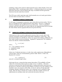
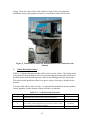
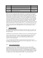
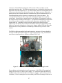
A Study of the Emissions from Diesel Vehicles
Operating in Xi’an, China
June 2008
Sebastian Tolvett, ISSRC
Huan Liu, Tsinghua University
Yingzhi Zhang, Tsinghua University
James Lents, ISSRC
Mauricio Osses, University of Chile
Kebin He, Tsinghua University
1
Table of Contents
I.
INTRODUCTION ................................................................................................................................................ 1
II.
TESTING PROCEDURE................................................................................................................................... 2
III.
MEASUREMENT ERROR.............................................................................................................................. 5
IV.
OVERALL RESULTS ...................................................................................................................................... 6
V.
VEHICLE EMISSIONS UNDER DIFFERENT DRIVING CONDITIONS .............................................. 14
VI.
EMISSION COMPARISONS WITH THE IVE MODEL .......................................................................... 16
VII.
CONCLUSIONS............................................................................................................................................. 18
List of Tables
TABLE 1: DIESEL VEHICLES TESTED DURING THE STUDY ............................................................................................. 1
TABLE 2: ESTIMATION OF EXPECTED VARIATION IN TEST DATA FOR REPEATED DRIVING CYCLES .............................. 5
TABLE 3: EMISSION MEASUREMENT RESULTS FOR THE TESTED XI’AN DIESEL FLEET.................................................. 6
TABLE 4: EMISSION MEASUREMENT RESULTS FOR THE TESTED XI’AN DIESEL FLEET (CONTINUED) ........................... 7
TABLE 5: POTENTIAL ADJUSTMENT VALUES TO BE USED IN IVE MODEL .................................................................. 17
TABLE 6: RECOMMENDED ADJUSTMENT VALUES FOR USE IN THE IVE MODEL .......................................................... 18
TABLE 7: EMISSIONS RESULTS FOR AN AVERAGE FLEET IN SEVERAL CITIES ................................................................ 18
List of Figures
FIGURE 1: ISSRC FIELD DILUTION DEVICE ................................................................................................................... 3
FIGURE 2: FLOW DIAGRAM FOR THE OVERALL EMISSIONS TESTING SYSTEM ............................................................... 3
FIGURE 3: EXTERIOR OF A TRUCK OUTFITTED FOR EMISSIONS TESTING ....................................................................... 4
FIGURE 4: WATER BARRELS FOR EMISSIONS TESTING .................................................................................................. 4
FIGURE 5: NUMBER OF VEHICLES BY MODEL YEARS FOR THE TESTED LIGHT DUTY TRUCKS (G/KM)........................... 8
FIGURE 6: EMISSIONS AVERAGED OVER SELECTED MODEL YEARS FOR LIGHT DUTY (G/KM) ....................................... 8
FIGURE 7: VEHICLES DISTRIBUTION ACCORDING TO EMISSIONS STANDARD ................................................................. 9
FIGURE 8: FTP NORMALIZED EMISSIONS AVERAGED OVER EMISSIONS STANDARDS OVERALL ................................. 10
FIGURE 9: VEHICLES DISTRIBUTION ACCORDING TO WEIGHT...................................................................................... 11
FIGURE 10: FTP NORMALIZED EMISSIONS AVERAGED OVER VEHICLE WEIGHT ......................................................... 11
FIGURE 11: VEHICLES DISTRIBUTION ACCORDING TO MILEAGE .................................................................................. 12
FIGURE 12: FTP NORMALIZED EMISSIONS AVERAGED OVER VEHICLE MILEAGE ....................................................... 13
FIGURE 13: FRACTION OF DRIVING IN VARIOUS BINS .................................................................................................. 14
FIGURE 14: CO2 EMISSIONS FROM LIGHT DUTY VEHICLES BY IVE BIN ..................................................................... 14
FIGURE 15: NOX EMISSIONS BY IVE BIN .................................................................................................................... 15
FIGURE 16: PM EMISSIONS BY IVE BIN ....................................................................................................................... 15
FIGURE 17: COMPARISON OF MEASURED EMISSION RATES WITH IVE PREDICTED EMISSION RATES .......................... 17
FIGURE 18: COMPARISON OF MEASURED EMISSION IN SEVERAL CITIES NORMALIZED TO THE FTP(LA4) CYCLE AND
GROUPED TO SIMILAR SIZE DISTRIBUTIONS ....................................................................................................... 19
2
I.
Introduction
From April 4 to May 9, 2008 a series of 40 diesel vehicles were tested in Xi’an China. All of
these vehicles were classified as light-heavy-duty vehicles. The tests were carried out in Xi’an at
a laboratory in Shaanxi University of Science and Technology. Table 1indicates the vehicles
that were tested.
Table 1: Diesel Vehicles Tested During the Study
Test
Number
Vehicle Type
Model
Emission Standard
Year
Odometer
(km)
Size
(kg)
1
Light Truck
JIEFANG
Euro 2
2005
47485
2480
2
Light Truck
JINBEI
Euro 2
2007
24000
2480
3
Light Truck
FUTIAN
Euro 1
2003
129578
2430
4
Light Truck
KAIMA
Euro 2
2007
20282
2790
5
Light Truck
LANLING
Euro 1
2001
230000
3100
6
Light Truck
JIANGHUAI
Euro 2
2008
7617
2495
7
Light Truck
JINBEI
Euro 2
2007
45678
2360
8
Light Truck
YUEJIN
Euro 0
1999
264945
2450
9
Light Truck
YUEJIN
Euro 2
2005
107805
3470
10
Light Truck
YUEJIN
Euro 2
2007
8184
2680
12
Light Truck
JINBEI
Euro 2
2007
32863
2340
11
Light Truck
YUEJIN
Euro 2
2005
65731
2165
13
Light Truck
YUEJIN
Euro 2
2007
9776
3710
14
Light Truck
JINBEI
Euro 1
2002
163468
1950
15
Light Truck
JIANGHUAI
Euro 1
2001
234500
4000
16
Light Truck
YUEJIN
Euro 2
2007
18546
2680
17
Light Truck
JINBEI
Euro 2
2007
25725
2500
18
Light Truck
JIEFANG
Euro 2
2006
75000
3240
19
Light Truck
YUEJIN
Euro 2
2005
71951
2290
20
Light Truck
SHI DAI
Euro 2
2007
35000
2070
21
Light Truck
JINBEI
Euro 1
2002
156135
3890
22
Light Truck
JINBEI
Euro 2
2008
3654
2340
23
Light Truck
JINBEI
Euro 2
2008
4753
2810
24
Light Truck
FUTIAN
Euro 1
2002
116695
2200
25
Light Truck
QINGQI
Euro 1
2002
172691
2450
26
Light Truck
JINBEI
Euro 2
2008
5765
4295
27
Light Truck
JIANGHUAI
Euro 2
2007
40077
3295
28
Light Truck
SHIHUA
Euro 2
2005
62524
2360
29
Light Truck
FUTIAN
Euro 1
2003
167155
4000
30
Light Truck
SHIDAI
Euro 2
2007
18833
2690
31
Light Truck
YUEJIN
Euro 2
2005
115075
2170
32
Light Truck
YUEJIN
Euro 2
2008
1623
2080
33
Light Truck
YUEJIN
Euro 1
2004
91743
3815
34
Light Truck
JIANGHUAI
Euro 1
2001
211500
5750
35
Light Truck
JIANGHUAI
Euro 2
2006
43968
3295
36
Light Truck
DONGFENG
Euro 2
2006
53887
4200
37
Light Truck
DONGFENG
Euro 2
2004
73125
4420
38
Light Truck
DONGFENG
Euro 1
2002
206809
4170
39
Light Truck
YUEJIN
Euro 2
2007
24525
2895
40
Light Truck
Euro 1
2003
87397
4661
1
This study was a joint effort of the Tsinghua University and the International Sustainable
Systems Research Center (ISSRC).
II.
Testing Procedure
Vehicles were brought to the test site by drivers supplied by the owners of the vehicles for test
equipment installation. These vehicles were warmed up at the time of the testing. Once the
emissions testing equipment was installed, the vehicles were driven over a prescribed driving
circuit by the original vehicle drivers. The driving route was designed so that the vehicles would
be operated over as wide a range of operating conditions as could be achieved within the city
limits of Xi’an. The driving circuit required from 30 to 40 minutes to complete depending upon
the traffic situation and included a moderate hill that the vehicles drove over.
For emission measurement purposes, a Semtech Sensor D gas emissions testing unit was used to
measure the emissions of CO, CO2, total Hydrocarbons (THC), NOx, and NO2. The Sensor D
unit uses infrared absorption technology to measure CO and CO2 , ultraviolet absorption
technology to measure NOx and NO2, and a flame ionization detector to measure total
hydrocarbon emissions. The Sensor D testing unit is an integrated emissions testing device
designed to be used in on-road testing programs. The Sensor D measures emission
concentrations and must be provided with exhaust flow rates and ambient temperatures and
pressures in order to determine mass emission rates. The Sensor D is equipped with a
temperature/pressure sensor. A Semtech manufactured 4 inch (10 cm) exhaust flow
measurement device was used to measure the exhaust flow rate from the vehicles. This device
uses standard dynamic and static pressure measurement techniques to calculate exhaust flow.
The Sensor D was also equipped with a GPS device to measure location and speed. All data
were collected at one second intervals. For further information on the Sensor D test unit and the
Semtech exhaust flow device please go to www.sensors-inc.com . The Sensor D test unit was
zeroed and spanned at each set of test cycles. The unit was found to be very stable from day to
day with the zero and span holding within 1% of the calibration gases values from day to day.
Particulates were measured on a second by second basis using a Dekati DMM testing unit. This
unit uses a particle charging process and six stage impactor setup to determine particle mass.
The DMM measures particle concentration. The exhaust flow rates collected by the Sensor D
unit must be used with the Dekati measurements to determine particulate mass flow rates. The
DMM measures particles in the 0 to 1.5 micron range, which is the size range where virtually all
diesel particulates reside. The DMM has been found to produce results comparable to the
reference particulate sampling methods for diesel particulates; although, it was found to produce
readings about 30% high in one published study. Dekati experts believe that this is due to the
fact that the Dekati measurement process can measure volatile particulate matter that is lost in
the case of filter based particulate sampling devices. For further information on the DMM,
please see www.dekati.com. The DMM was zeroed at the beginning of each testing cycle. The
charging and impactor units become covered with particulates and must be cleaned after each 2-3
hours of testing to keep the unit operating properly.
2
The DMM can not handle the mass concentrations found in uncontrolled diesel exhaust. Thus,
the diesel exhaust must be diluted at a controlled rate in order to use the DMM. A field dilution
device was developed by ISSRC to use in on-road emissions testing with the DMM. Figure 1
illustrates the design of the ISSRC field dilution unit.
Figure 1: ISSRC Field Dilution Device
The exhaust flow in the dilution device is measured using a Dwyer differential pressure
transducer, which is accurate to 0.25% of full scale. The differential pressure gauge is used to
measure the pressure difference between P2 and P3 shown in Figure 1. A micro-filter produces
particle free air to be diluted with the exhaust sample. The exhaust sample and dilution air are
heated to 110 degrees C to avoid water and organic condensation. The dilution level reaches
values from 20 to 1 to 30 to 1 depending on the vehicle tested and the exhaust flow rate.
Figure 2 presents a flow diagram for the overall emissions testing system. The data collected by
Figure 2: Flow Diagram for the Overall Emissions Testing System
the flow measurement device and the Sensor D are recorded to a flash card on the Sensor D unit.
The Dekati information is recorded to a laptop computer that is connected to the Dekati by a
serial cable.
3
Figure 3 and Figure 4 show the exterior of a truck outfitted for testing.
Figure 3: Exterior of a Truck Outfitted for Emissions Testing
Figure 4: Water Barrels for Emissions Testing
4
In order to simulate a loaded truck, 200 Kilograms of water in barrels were placed on the truck
according to the carrying capacity of the truck. Depending upon the size of the vehicles, barrels
were loaded to simulate 50% of the total load capacity to produce consistent measurements.
Appendix A contains a description of the overall testing procedure and data processing steps.
III.
Measurement Error
No measurement process is free from measurement and operating error. Referring to Figure 2,
there is the potential for measurement error in the flow measurement process, the dilution rate
measurement, the gas concentrations measurement. Table 2 outlines potential error assuming
that each process can be held to produce only 2% error to help understand the expected
variations in results from the repeated testing.
Table 2: Estimation of Expected Variation in Test Data for Repeated Driving Cycles
Impact on Gaseous
Measurements
2%
--2%
4%
Measurement Process
Exhaust Volume Flow Measurement
Dilution Measurement
Emissions Concentration Measurement
Total Potential Variation
Impact on Particle
Measurements
2%
2%
2%
6%
To further complicate the process, data is collected on normal city streets which results in
different driving patterns from test to test. Daily variations in traffic flow have a major impact
on how the vehicles can be operated. Thus, emissions can vary considerably from test to test
even using the same vehicle. To correct for this variation, the data is divided into different
power demand categories. 60 power demand categories are used for this purpose. These
categories are typically referred to as Power Bins and are numbered from 0 to 59. The amount of
emissions that occurs when the vehicle is operated in each of the 60 Power Bins is determined.1
This bin emission rate is multiplied by the driving distribution that would have occurred had the
vehicle driven an FTP driving cycle to produce a standardized estimate of emissions that would
have resulted if the vehicle had been operated on an FTP cycle. This approach was found in an
already published study in Brazil to produce estimates of emissions on the actual driving cycle
within 6%. While this is good in many respects, it must be added to measurement uncertainty
indicated in Table 2, which results in a potential emissions error of 10-12% overall. The error
discussed in the previous paragraphs should be random and thus should average out to some
degree over multiple tests.
Finally, the number of vehicles that can be tested in a 2 week period is limited. This limited
testing further decreases the certainty of how well the tested fleet actually represents the actual
urban fleet. Based on ISSRC data collected in similar gasoline emissions studies, the collection
1
A vehicle will typically not operate in all of the defined Power Bins during a given driving test. Since this data is
only used to calculate emissions projected for an FTP cycle, it is only important to have values for the bins that
occur in the FTP cycle. This usually occurs. In the few cases were a FTP bin is missing, then the data is
interpolated to fill in values.
5
of data from a fleet of randomly selected gasoline fueled vehicles resulted in 90% confidence
interval of plus or minus 20%.
When all potential errors are combined, it should be anticipated that this study will produce
results which are to a 90% probability to within 20-30% of the actual emissions produced by the
local fleet. While this potential error is larger than preferred, it is still better than using emission
estimates derived from studies in the U.S. and Europe. In the long run, more emissions tests are
required in order to reduce the mobile source inventory uncertainty to the more preferred 10%
range.
IV.
Overall Results
Table 3 and Table 4 present the average emissions measured for the various vehicles tested in the
program. They are listed in the order tested. An average value and 90% confidence limits are
also included at the end of Table 4. The 90% confidence interval in Table 4 indicates the range
of emissions for which there is a 90% probability that the true mean emission rate of the fleet
would exist if the tested vehicles were randomly selected from the Xi’an fleet. The vehicles
tested should be somewhat representative of the Xi’an fleet, thus, the measured values are likely
within 20-25% of the true mean of the Xi’an fleet. It should be noted that any zero emissions
shown in Tables 3 or 4 indicates that emissions measured for the vehicles were below the
detection limits of the equipment. This only occurs in the case of CO and THC due to the fact
that diesel vehicles run with high amounts of air compared to the fuel and a well running engine
can have low CO and THC.
Table 3: Emission Measurement Results for the Tested Xi’an Diesel Fleet
Test
Vehicle Type Year
Number
1
Light Truck
2
Light Truck
3
Light Truck
4
Light Truck
5
Light Truck
6
Light Truck
7
Light Truck
8
Light Truck
9
Light Truck
10
Light Truck
11
Light Truck
12
Light Truck
13
Light Truck
14
Light Truck
15
Light Truck
16
Light Truck
17
Light Truck
18
Light Truck
19
Light Truck
20
Light Truck
Measured Emissions
(grams/kilometer)
Std
FTP Normalized Emissions
(grams/kilometer
CO2
NOx
PM
CO
THC
CO2
NOx
PM
CO
THC
2005 Euro 2
2007 Euro 2
341
5.62
0.325
10.93
1.93
401
7.74
0.392
13.25
2.16
283
3.42
0.071
1.60
1.19
336
4.70
0.088
1.97
1.38
2003 Euro 1
2007 Euro 2
253
2.83
0.245
3.26
1.59
294
3.87
0.294
3.92
1.77
430
10.83
0.066
1.96
1.98
396
13.56
0.063
1.86
1.56
2001 Euro 1
2008 Euro 2
284
3.23
0.359
3.63
1.48
350
4.64
0.458
4.64
1.79
275
4.25
0.148
5.63
1.38
328
5.50
0.179
6.88
1.64
2007 Euro 2
1999 Euro 0
394
5.99
0.294
12.35
2.33
360
6.97
0.251
10.59
1.87
298
2.99
0.496
14.63
2.28
296
3.83
0.504
14.99
2.02
2005 Euro 2
2007 Euro 2
314
4.43
0.116
3.15
1.34
381
5.90
0.146
3.96
1.63
246
4.51
0.090
1.31
1.29
281
6.11
0.106
1.54
1.40
2007 Euro 2
2005 Euro 2
266
5.16
0.058
1.39
1.26
305
6.74
0.065
1.56
1.39
229
4.54
0.085
1.32
1.56
226
5.87
0.080
1.24
1.33
2007 Euro 2
2002 Euro 1
329
4.98
0.101
1.68
1.78
381
6.56
0.121
2.00
2.00
342
7.04
0.172
7.83
1.32
380
8.56
0.198
8.95
1.44
2001 Euro 1
2007 Euro 2
305
5.79
0.080
3.60
2.15
371
7.82
0.098
4.41
2.60
265
4.52
0.209
2.66
1.27
309
5.66
0.246
3.13
1.47
2007 Euro 2
2006 Euro 2
288
4.03
0.122
4.28
1.34
332
5.27
0.146
5.11
1.51
223
3.91
0.042
1.02
0.63
269
5.17
0.052
1.26
0.75
2005 Euro 2
2007 Euro 2
319
10.04
0.075
1.69
1.07
362
12.50
0.086
1.91
1.18
283
5.67
0.369
7.16
1.45
338
7.64
0.454
8.82
1.68
6
21
Light Truck
2002 Euro 1
351
8.78
0.245
13.60
1.58
403
10.09
0.281
15.79
1.80
Table 4: Emission Measurement Results for the Tested Xi’an Diesel Fleet (continued)
Test
Vehicle Type Year
Number
CO2
Measured Emissions
(grams/kilometer)
NOx
PM
CO
THC
CO2
Std
FTP Normalized Emissions
(grams/kilometer
NOx
PM
CO
THC
22
Light Truck
2008 Euro 2
301
3.20
0.161
2.36
0.69
353
4.04
0.193
2.86
0.80
23
Light Truck
2008 Euro 2
288
7.63
0.047
1.99
1.07
361
10.49
0.061
2.57
1.33
24
Light Truck
2002 Euro 1
282
3.52
0.673
2.43
1.74
344
4.79
0.846
3.06
2.13
25
Light Truck
2002 Euro 1
351
3.55
0.180
6.75
2.11
346
4.18
0.182
6.83
1.93
26
Light Truck
2008 Euro 2
336
5.63
0.173
2.15
1.45
425
7.81
0.216
2.70
1.79
27
Light Truck
2007 Euro 2
444
4.60
0.156
4.01
1.68
482
5.52
0.174
4.48
1.79
28
Light Truck
2005 Euro 2
353
9.00
0.076
1.95
1.19
419
12.28
0.093
2.37
1.37
29
Light Truck
2003 Euro 1
295
5.94
0.206
7.73
1.76
333
7.73
0.233
8.74
1.91
30
Light Truck
2007 Euro 2
269
2.90
0.266
4.45
1.30
306
3.82
0.312
5.20
1.43
31
Light Truck
2005 Euro 2
251
4.24
0.103
1.86
1.37
282
5.32
0.119
2.16
1.54
32
Light Truck
2008 Euro 2
294
5.06
0.011
1.46
1.22
368
6.51
0.014
1.77
1.55
33
Light Truck
2004 Euro 1
237
5.52
0.001
3.26
1.26
305
7.55
0.001
4.24
1.67
34
Light Truck
2001 Euro 1
287
4.94
0.160
4.14
1.71
332
5.87
0.155
4.03
1.98
35
Light Truck
2006 Euro 2
366
6.77
0.107
3.41
1.60
380
7.99
0.115
3.61
1.58
36
Light Truck
2006 Euro 2
328
7.76
0.082
1.12
0.52
397
10.07
0.101
1.39
0.62
37
Light Truck
2004 Euro 1
357
5.63
0.111
1.07
0.53
418
7.01
0.132
1.29
0.62
38
Light Truck
2002 Euro 2
339
5.89
0.116
1.29
0.43
417
7.64
0.148
1.63
0.55
39
Light Truck
2007 Euro 2
237
2.90
0.081
0.54
0.97
281
4.00
0.099
0.65
1.12
CO2
NOx
PM
CO
THC
CO2
NOx
PM
CO
THC
Average of Tests
305.92
5.31
0.17
4.02
1.40
349.95
6.85
0.19
4.55
1.54
90% Confidence Interval
4%
10%
21%
24%
9%
4%
9%
22%
22%
8%
Emissions according to Model Year
Figure 5 shows the Model Year distribution of the sampled vehicles in this study. There were 4
(10%) of the vehicles in the range of years 1999-2002, 9 (23%) were in the 2002-2005 range and
26 (67%) were in the 2005-2008 year range.
Figure 6 shows the CO, HC, NOx, PM and CO2 emissions from the Light Duty Trucks and
emissions for three groupings of model years, as can be seen in Figure 5. There is a little overall
relation between emissions and model year for the vehicles tested in China. CO, THC and PM
show a decrease trend. NOx shows a growing trend in emissions. Because the newer vehicles,
the higher NOx emissions.
7
2009
1999
2008 -2002
2005-2008
2002-2005
2007
2006
MODEL YEAR
2005
2004
2003
2002
2001
2000
1999
1998
1
6
11
16
21
26
31
36
Figure 5: Number of Vehicles by Model Years for the Tested Light Duty Trucks (g/km)
7.00
6.50
1999-2001
6.00
2002-2004
5.41
5.25
5.45
2005-2008
5.00
Emission [g/km]
4.24
4.00
3.21
2.93
3.00
3.12
3.06
2.74
2.17
1.91
2.00
1.37
1.34
1.32
1.00
0.00
CO
CO2/100
NOx
THC
PM*10
Figure 6: Emissions Averaged over Selected Model Years for Light Duty (g/km)
8
Emissions according to Emissions Standard
Figure 7, shows the distribution of the sampled vehicles. All of the vehicles are, of course, Light
Duty Trucks. In addition, one vehicle (3%) complies the Euro 0 standard, 11 vehicles (28%)
complies Euro 1 standard, 27 (69%) complies Euro 2.
1, 3%
Euro0
Euro1
Euro2
11, 28%
27, 69%
Light Trucks
Figure 7: Vehicles Distribution According to Emissions Standard
Figure 8, shows the emissions results for CO, HC, NOx, PM and CO2, distributed by the vehicle
engine standards.
The Overall results show a reasonable correlation with the standard looking from Euro 1 through
Euro 2 standards, indicating a reduction for CO, THC, and PM10. The Euro 0 vehicle shows
high levels of emissions for CO, THC and PM, but it shows lower levels of emissions for CO2
and NOx. It appears that the Euro 0 vehicle’s engine size is smaller than the others.
Observing results there is a relationship between emissions and engine standard except for NOx
and CO2 where there is little improvement between Euro 1 and Euro 2. The Euro 1 NOx
emissions are lower than the Euro 2 for trucks with the same engine sizes.
In summary, the results show a good relationship between emissions and standard except for
NOx. It should be noted that just one Euro 0 truck was tested in Xi’an. Thus, this emission rate
should not be given much consideration.
9
18.00
16.00
Euro 0
14.99
Euro 1
14.00
Euro 2
Emission [g/km]
12.00
10.00
8.00
6.61
6.02
7.06
6.00
5.04
3.56
4.00
2.96
3.52 3.51
3.83
2.02 1.78
1.42
2.00
2.63
1.52
0.00
CO
CO2/100
NOx
THC
PM*10
Figure 8: FTP Normalized Emissions Averaged Over Emissions Standards Overall
Emissions according to Weight
In Figure 9 the Weight distribution of the vehicles tested is shown, the range for the overall
sample is only 5 tons, between 1 to 6 Tons. In the range of 1 to 4 tons, there were 34 vehicles, 23
of them between 2 and 3 tons. In the range of 4 to 6 tons, there are only 5 vehicles.
The vehicles were grouped into two weight classes. In Figure 10 the results of emissions for
these two weight classes are shown. The CO, THC and PM emissions become lower when the
weight increases. These can be explained because the heavy vehicles tended to be newer. The
CO2 and NOx emissions of the high weight range vehicles are slightly higher than the lighter
ones. The reason for this is that the lighter vehicles have smaller engines than heavier ones, and
the bigger engine has the higher CO2 emission.
10
7.0
1T-4T
4T-6T
6.0
Weight[tons]
5.0
4.0
3.0
2.0
1.0
0.0
1
6
11
16
21
26
31
36
Figure 9: Vehicles Distribution According to Weight
9.00
7.71
8.00
4-6[Tons]
6.67
7.00
Emission [g/km]
1-4[Tons]
6.00
5.00
4.00
4.79
3.46
3.42
3.85
3.00
1.56 1.44
2.00
2.01
1.55
1.00
0.00
CO
CO2/100
NOx
THC
PM*10
Figure 10: FTP Normalized Emissions Averaged Over Vehicle Weight
Emissions according to mileage
In Figure 11 the distribution according to mileage is shown. The range of mileage is going
between 0 to 300,000 kilometers. The distribution shows 25 (64%) of the vehicles in the low
range 0 to 80,000 kilometers, 6 (15%) in the middle range 80,000 to 160,000 kilometers and 8
(21%) in the high range 160,000 and more.
11
The results in Figure 12 show the emissions by mileage distribution of the trucks. There is some
relationship between mileage and emissions, NOx emissions seem to almost the same in the
middle and high range, and it is higher in the low range than the others. CO and HC emissions
are higher as the mileage increases. CO2 emissions show lower emissions on the middle range of
mileage and higher in the high and low range of mileage. PM emissions show higher emissions
on the middle range of mileage and lower in the low range of mileage. Again, vehicle size is not
equal throughout the size range complicating the picture and illustrating the need for a broad
range of vehicle testing.
300000
X<80,000
80,000<x<
160,000
x>160,000
250000
Mileage [km]
200000
150000
100000
50000
0
1
6
11
16
21
26
31
Figure 11: Vehicles Distribution According to Mileage
12
36
8.00
7.18
x<80,000
6.78
7.00
80,000<x<160,000
6.25 6.28
Emission [g/km]
6.00
6.25 6.28
x>160,000
5.52
5.00
4.00
3.60
3.53
3.35
3.53
2.81
3.00
2.47
2.00
1.54
1.41
1.00
0.00
CO
CO2/100
NOx
THC
PM*10
Figure 12: FTP Normalized Emissions Averaged Over Vehicle Mileage
13
V.
Vehicle Emissions Under Different Driving Conditions
Another purpose of this study is to determine how emissions vary under different driving
conditions. These conditions can be represented by the IVE driving bin designations. The IVE
model divides the range of driving situations into 20 vehicle energy demand situations2 and 3
engine stress situations3. Figures 13, 14, 15 and 16 present emissions from the diesel vehicles as
a function of IVE driving bin.
0.45
Driving Bins
0.4
0.35
(%)
0.3
0.25
0.2
0.15
0.1
0.05
0
1.00 1.03 1.06 1.09 1.12 1.15 1.18 2.01 2.04 2.07 2.10 2.13 2.16 2.19 3.02 3.05 3.08 3.11 3.14 3.17
Figure 13: Fraction of Driving in Various Bins
CO2
8
7
(g/km)
6
5
4
3
2
1
0
1.00 1.03 1.06 1.09 1.12 1.15 1.18 2.01 2.04 2.07 2.10 2.13 2.16 2.19 3.02 3.05 3.08 3.11 3.14 3.17
Figure 14: CO2 Emissions From Light Duty Vehicles by IVE Bin
The emissions look typical with the exception of the apparent fall off in emission rates in stress
category 1 in the case of bins 15-19 (i.e. 1.15 to 1.19 in Figures 14, 15, and 16). Reviewing
Figure 13 there are many seconds of data in the bins 9-15 (i.e. 1.09 to 1.15 in Figures 14, 15, and
16). There is very little data in bins 15-19. This results in the classification of data into
erroneously high bins. It appears that momentary deviations in GPS altitude and speed produced
erroneous calculations of road grade and acceleration. It has been found that the GPS unit will
loose signal, freeze, and then jump to the correct speed a few seconds to a minute later when the
2
The energy demand on a vehicle is the result of engine and rolling friction, wind resistance, acceleration energy,
and road grade. For a further discussion, the reader is referred to the user’s manual for the IVE model, which can be
obtained at www.issrc.org/ive .
3
Engine stress relates to engine rpm and the average energy demand on the vehicle in the most recent 15 seconds.
The reader is referred to the user’s manual for the IVE model, which can be obtained at www.issrc.org/ive .
14
signal returns. Altitude can also be mis-measured by the GPS. Steps are taken to filter these
events out of the data; however, a few data points slip by. The data in bins 1.15-1.19 in Figure 6
represent only 0.001% of the collected data and are included only for the sake of completeness.
We believe that these data should be ignored.
In the case of bins 1-5 (i.e. 1.01 to 1.05 in Figure 6) the points are higher than normal. Due to the
emergency braking, it is likely that driving occurred in bins 1.01 to 1.05. In the course that we
drove in Xi’an there are a few speed bumps on the road, and the vehicles that we tested were
rapidly slowed down when they met the speed bumps to avoid damage to the testing equipment.
Figure 15 presents data from the same vehicles but this data is the NOx data from those vehicles.
NOx
0.14
(g/km)
0.12
0.1
0.08
0.06
0.04
0.02
0
1.00 1.03 1.06 1.09 1.12 1.15 1.18 2.01 2.04 2.07 2.10 2.13 2.16 2.19 3.02 3.05 3.08 3.11 3.14 3.17
Figure 15: NOx Emissions by IVE Bin
The main difference compared to previous studies of diesel vehicles is that there is a high
emissions rate in bins from 1.00 to 1.05, those bins represented the emissions on vehicles when
they are decelerating, and one of the possible causes of this behavior, as discussed earlier, is that
the vehicles were being rapidly slowed down when they met speed bumps.
Figure 16 presents the binned data for particulate matter from the large diesel vehicles. The
standard form of the emissions curve can still be seen in the data when the erroneous bin
classifications are ignored.
PM
0.0045
0.004
(g/km)
0.0035
0.003
0.0025
0.002
0.0015
0.001
0.0005
0
1.00 1.03 1.06 1.09 1.12 1.15 1.18 2.01 2.04 2.07 2.10 2.13 2.16 2.19 3.02 3.05 3.08 3.11 3.14 3.17
Figure 16: PM Emissions by IVE Bin
15
There is a consistent result for the low bins for the PM results; they have high emissions in bins
from 1.00 to 1.03, probably for the same cause that was already discussed with respect to the
CO2 and NOx. Emissions appear to be normal compared to measurements made in other cities.
VI.
Emission Comparisons with the IVE Model
As noted earlier, 39 trucks were successfully tested in Xi’an. This limited data does not provide
large enough samples of individual technologies to do an analysis of emission comparisons by
technology type. Instead, the IVE model was run using an FTP driving pattern, the pattern used
to develop base emission factors for the IVE model, and using the overall distribution of vehicles
tested in Xi’an. The average measured values normalized to FTP driving cycles were then
divided by the IVE predicted values to evaluate the comparisons. Figure 17 provides the results
of this analysis.
As can be seen, the CO2 emission projections were accurate producing a ratio close to 14. The
other predictions, however, showed a wide variance. The model appears to be underestimating
the emissions for all the vehicles except NOx and PM for Euro 0 and PM for Euro 1, but actually
they are almost the same between model prediction and measured value in NOx and PM for Euro
0. For Euro 1 and Euro 2 the model is overestimating the emissions for CO, HC and NOx.
4
The exact value for all the vehicles is 1.29.
16
12.00
10.00
8.00
E0
6.00
E1
E2
OA
4.00
2.00
0.00
CO Ratio
HC Ratio
NOx Ratio
PM Ratio
CO2 Ratio
Figure 17: Comparison of Measured Emission Rates with IVE Predicted Emission Rates
The default base emission factors in the IVE model are based primarily on emission
measurements made in the United States and Europe and represent test results from thousands of
vehicles. It is difficult to know how much weight to give to emission results from only 39
vehicles in Xi’an. However, the confidence limits shown in Table 3 suggest that the averages of
the results should be in the ballpark of 30% of the actual values. Table 5 shows the actual ratios
and the ratios of the measured emission results were modified to be 30% closer to the IVE
projected values.
Table 5: Potential Adjustment Values To Be Used in IVE Model
Standard
Euro 0
Euro 1
Euro 2
Overall
CO Ratio
2.43
7.17
5.74
5.61
HC Ratio
2.06
5.39
7.12
5.92
NOX Ratio
0.96
2.02
2.06
1.95
PM Ratio
0.98
0.52
2.17
0.96
CO2 Ratio
1.00
1.05
1.11
1.08
Because of the limited number of tests, it is suggested that the values closer to the IVE default
values (the 30% adjusted values) be used until more in-use emissions data is collected in Xi’an.
A value of 1 is used in the cases where the 30% adjustment takes the values from less than 1 to
greater than 1.
17
Table 6 presents the recommended adjustment values for diesel vehicles in Xi’an. These values
should, of course, be improved as more data is collected.
Table 6: Recommended Adjustment Values for Use in the IVE model
Class
Euro 0
Euro 1
Euro 2
Overall
VII.
CO Ratio
2.75
7.17
5.74
5.61
VOC Ratio
1.92
5.39
7.12
5.92
NOx Ratio
0.48
2.02
2.06
1.95
PM Ratio
1.26
0.52
2.17
0.96
Conclusions
In summary, the results of this report explain the relationship between the real emissions and the
estimated emissions as determined by the IVE model. However, this information is not complete
without comparing the emissions of the light duty fleet in Xi’an with others fleets around the
world.
The comparisons in this chapter include six cities: Beijing (China), Istanbul (Turkey), Mexico
City (Mexico), Santiago (Chile), Sao Paulo (Brazil) and Xi’an (China). In order to normalize the
results and make them comparable, the Bin methodology has been used to evaluate the emissions
of each city under the FTP (LA4) cycle. The comparison includes the overall emissions for each
campaign in each city. It has to be noticed that in the case of Santiago the Light Duty vehicles
are small diesel vehicle with less than 2.5 liter engines.
The Table 7 below displays the results.
Table 7: Emissions results for an average fleet in several cities
Pollutant
CO [g/km]
HC [g/km]
NOx [g/km]
PM*10 [g/km]
CO2/100 [g/km]
Xi’an
Beijing
Istanbul
Mexico
City
4.55
1.54
6.85
1.92
3.50
2.47
1.06
5.67
2.37
4.82
1.35
0.51
3.58
0.92
3.36
6.52
0.78
5.91
3.81
5.40
Santiago
Light
Duty
0.40
0.04
1.10
0.09
2.21
Santiago
Heavy
Duty
1.41
0.48
3.13
0.42
2.85
Sao Paulo
2.59
0.55
5.30
1.48
4.84
In Figure 19, the results are shown with the 90% confidence interval so that one can better
understand the variation in the measured data for each city and likely representativeness of the
data for each city.
18
10.00
9.00
8.00
Emissions [g/km]
7.00
Beijing
MexicoCity
Istanbul
SantiagoLD
SantiagoHD
Sao Paulo
Xi 'an
6.00
5.00
4.00
3.00
2.00
1.00
0.00
CO
HC
NOx
PM*10
CO2/100
Figure 18: Comparison of Measured Emission in Several Cities Normalized to the
FTP(LA4) Cycle and Grouped to Similar Size Distributions
After studying the results, it can be concluded that:
•
CO2 emissions from the trucks in Xi’an are comparable to those emissions found in vehicles
measured in Istanbul. However, the vehicles measured in Mexico City and Sao Paulo were
significantly larger than the Xi’an vehicles tested. This indicates that the Xi’an vehicles are
not very fuel efficient for their size.
•
HC and NOx emissions of the Xi’an vehicles are the highest in these cities, although ones
tested were not the largest ones.
•
PM emissions for Xi’an vehicles makes more sense. But it is higher than Sao Paulo. This is
especially worrisome considering that the Sao Paulo vehicles were significantly larger than
the Xi’an vehicles.
•
CO emissions are the second greatest of the cities studied. They are higher than Beijing
vehicles which are bigger in size than Xi’an vehicles.
An analysis was also done to derive the rates of emission increase with vehicle use. However, as
was the case with model year comparisons, the measurements did not show a trend of vehicle
emissions increasing with use. This is an unusual result, but may be because the fleet tested in
Xi’an was relatively homogeneous.
The fact that emissions from the Xi’an diesel vehicles seem to run higher than comparable
vehicles in the other cities tested may suggest that maintenance in Xi’an may be lax. It might be
good to establish a traditional Inspection and Maintenance program for vehicles or to use remote
19
sensing to measure the emission rates of trucks as they transverse the city to identify and repair
high emitters. In addition, some differences of emissions were found among vehicles supposedly
conforming to different vehicle emission standards, which mean there is effective emission
improvement for diesel trucks in Xi’an during in recent years with tightening emission standards.
Particulate and NOx control devices are becoming available for reducing diesel emissions. Xi’an
may want to take advantage of these controls by setting more stringent new vehicle standards
and by considering some form of retrofit program for diesel vehicles.
20
Appendix A
Field Manual For Diesel Vehicle Testing
21
IVE In-Use Vehicle Emissions Study for Diesel Vehicles
I. Introduction:
Diesel emissions are important contributors to air quality degradation in urban areas.
Diesel particulates are considered to be carcinogenic or likely carcinogens in the United
States, and diesels are often the prime source of nitrogen oxide emissions. It is thus
important that diesel emissions be well understood and that air quality planners be able to
predict the impact of diesels in the present time and at times in the future based on
specific control scenarios. To support these efforts, a process of on-road measurement of
diesel emissions has been devised and the International Vehicle Emissions (IVE) model
was developed to estimate emissions from diesel vehicles under different driving and
control scenarios.
The IVE model is designed to make estimates of in-use vehicle emissions in the full
range of global urban areas. At the point in time of IVE model development, data to
establish base emission factors and driving pattern adjustments were, of necessity, based
on vehicle studies carried out primarily in the United States. This has raised questions as
to the applicability of the base emission rates and driving pattern adjustments used in the
model to developing countries. The IVE in-use vehicle emissions study is designed to
test the hypothesis that similar vehicle technologies will produce equivalent emission
results in a given location and to provide some rudimentary data for creating improved
emission factors.
The IVE modeling framework provides the user with the ability to enter adjustments to
the base emission factors that are specific to a location in case the supplied factors are
found to be in error. This capability was built into the model to support emission
measurement studies that would be made in developing countries as local capacity
increases. The IVE In-Use vehicle emissions study is not designed to fully develop
correction factors for the IVE model. The original data base used to developed the IVE
model correction factors was based on more than 500 vehicle tests each involving three
driving cycles carried out at the University of California CE-CERT research facility.
This information was combined with summarizations of thousands of in-use vehicle tests
provided by the United States Environmental Protection Agency. The IVE In-Use
emissions study discussed in the following section results in emissions data for 40 diesel
fueled vehicles. Information from 40 vehicles, while significant, does not provide the
range of data for the development of a full range of new emission factors and
adjustments. Nonetheless, the IVE In-Use emissions study can be used to make
rudimentary adjustments to the IVE model that will certainly improve its performance for
developing countries.
The actual IVE In-Use vehicle emissions study makes use of recently developed
emissions measurement technology that can be carried on-board vehicles while they are
driven on urban streets. This technology allows emission mass per unit distance to be
determined in real driving situations. To date, this on-board emissions measurement
22
technology can be used to measure carbon monoxide (CO), carbon dioxide (CO2), total
hydrocarbons (THC), and nitrogen oxides (NOx). A different testing device to measure
particulate emissions is also used during the study to establish real-time particulate
emissions from the tested diesel vehicles.
The IVE in-use vehicle emissions study is built around a two week study period where
on-road vehicle emissions data is collected.
II.
Equipment Needed to Complete Study
A wide range of equipment is required to carry out the diesel emissions study. The key
pieces of equipment will be shipped from the United States. However, a significant
amount of equipment and supplies must be provided locally. An Excel spreadsheet
program is provided with this write-up that indicates the equipment that will be sent from
the United States and the equipment that must be procured locally.
III.
Sample Size and Impact on Emissions Measurement Reliability:
Unfortunately for the researcher studying the emissions from on-road vehicles, the
variance in emissions among vehicles with similar technologies is quite large. This
means that multiple tests on different vehicles are required to accurately establish the true
fleet wide average for a given technology. Equation II.1 indicates the 70% confidence
interval for data in a Gaussian distribution.
I70% = ± σ/√ (n-1)
II.1
where,
I70% = 70% confidence interval
σ = standard deviation
n = sample size
In the case of vehicular emissions, σ is often close to the sample mean; although diesel
vehicles show a little less variation that do gasoline fueled vehicles. In this case,
Equation II.1 becomes:
I70% = ±[M/√(n-1)]
where M = measured sample mean
II.2
In this special case, to insure that the measured mean has a 70% probability of being
within 15% of the actual mean requires a sample size of 44 vehicles. The actual
variation in emissions from similar technologies is unknown but based on the previous
discussion it is clear that a relatively large number of vehicles of a given technology class
should be tested. For purposes of this study, at least 10 vehicles of each important
technology should be measured to insure even a moderate level of confidence in the
results. Once the data is collected, the variance in the data of similar vehicles will
establish the true confidence that can be placed in the results of the tests.
23
With present vehicle testing technology, about 1.5 hours are required to remove the
equipment from one vehicle and install the sampling equipment in a second vehicle. To
collect data for ¾ of an hour for a given vehicle will thus require a total of 2.25 hours per
vehicle. In a 9 hour day, about 4 vehicles can be sampled. In a two week sampling
period (10 sampling days), about 40 vehicles can be studied. Thus, based on the
preceding discussion, only four general vehicle technology groups should be studied over
the two week sampling period in order to insure at least 10 vehicles per technology class
are studied. The variety of diesel engine technologies operating in most urban areas
today are relatively small and the study of the four most predominate vehicle
technologies in an area will provide useful data for understanding the overall diesel
emissions in an urban area.
IV.
Sampling Program:
Based on Section II, it is desired to study four vehicle technology classes during the two
week study. The vehicle technology classes that should be studied are those groups
which dominate the local diesel fleet being studied and which will continue to be
important in the next 5 years. The vehicles selected may vary from location to location,
but based on previous experience, it is suggested that the following four technology
classes be considered:
1.
2.
3.
4.
Euro 1 type technologies
Euro 2 type technologies
Euro 3 type technologies
Euro 4 type technologies if available or extend testing of most common of
the three previous groups.
The previous suggested technology classes should not be rigidly adhered to in cases
where the local fleet does not contain significant numbers of vehicles in any of the
vehicle classes listed. It is best to tailor the study to the makeup of the local fleet. For
this paper, the four suggested classes will be used for discussion purposes.
Start emissions are important for gasoline vehicles but are not considered as important for
diesel vehicles. Thus the testing program that will be used will not collect diesel vehicle
start emissions. Vehicles will be scheduled to be brought to the testing area at 2.25 hour
intervals beginning at 08:00. Thus a second vehicle will be due at 10:15. (On the first
day only two tests should be scheduled to allow for proper on-site training.) It is critical
that vehicles not arrive late. It is best to schedule them to arrive a little early. The new
vehicles will be parked in the test area leaving room for the returning vehicle to be
parked. Once the vehicle being tested arrives at the test setup facility, the equipment is
moved from the tested vehicle and installed in the new vehicle that has arrived for testing.
Buses are expected to arrive with only a driver. Sand bags will be loaded onto the bus to
simulate passenger weight. Trucks should arrive with a half to a full load for purposes of
24
testing. The truck or bus will be at the facility for about 3 hours for equipment
installation, testing, and equipment removal. It can then be returned to its owner.
Figure 1: Truck and Bus with Flow Measurement Devices Connected to the
Exhaust
V.
Vehicle Driving Procedure:
Table IV.1 indicates the approach that will be used to test the vehicle. The driving roads
selected for the study should provide for convenient stopping locations that will occur at
the desired time intervals and return the vehicle to the starting point at the desired time.
The roads selected should also allow for as great a variety of driving as feasible for the
location.
It is critical that vehicles arrive on time. A testing facilitator should be in touch with the
vehicle suppliers to insure that the vehicles will arrive on schedule.
Table IV.1: Vehicle Driving Procedure
Step
1
2
3
4
Procedure
A vehicle arrives at the test setup facility at the designated
appointment time while previous vehicle is being tested.
Vehicle will be parked in the next vehicle test setup location
Vehicle will be studied and a decision will be made as to the best
way to attach testing equipment to the just arrived vehicle. Sand
bags are loaded onto vehicle to be tested.
Tested vehicle returns to the test setup location and parks near the
25
Time Interval
---5 minutes
20 minutes
5 minutes
5
6
7
8
9
next vehicle setup location.
Download data from the just tested vehicle
Test equipment is removed from tested vehicle and transferred to
new vehicle and tested vehicle released for return to the owner.
Equipment installed on new vehicle.
Data collection initiated and vehicle started and driven over the
designated one-hour test route.
Total time to test one vehicle
5 minutes
30 minutes
25 minutes
45 minutes
135 minutes
Traffic will of course impact the distances that will be covered during the driving phase.
Thus, the test route should be designed so that there are alternate routes to be taken so
that the vehicle can complete its test run in the 45 minutes that are allocated. Since traffic
will flow better at various times of the day, the test may be completed in 30 minutes in
one case and in 60 minutes in another case. The test route should be selected so that the
vehicle can complete the test run in 60 minutes in the worst traffic. It is also critical that
the driving course selected contain street sections where higher speeds and accelerations
can be achieved as well as slower speeds and lower accelerations. The driver should
operate the vehicle in a manner typical of the traffic that is occurring at the time of testing
and in the manner that the vehicle is normally used (i.e., a bus will stop at bus stops even
though it does not pick up or discharge passengers). Buses and trucks should be marked
with signs taped to the vehicle indicating that the vehicle is participating in a testing
program.
VI.
Vehicle Procurement:
Procuring 40 large diesel vehicles for testing with a driver and, in the case of trucks, can
be a challenge. Bus companies must be contacted as well as trucking companies to find
the desired vehicles.
In both Mexico City and Sao Paulo, a $US50 per vehicle fee was paid for gasoline fueled
vehicle. This fee plus the use of contacts at the partnering agencies provided all of the
needed vehicles in Sao Paulo. In the case of buses and trucks a higher fee may be
necessary unless representative buses can be obtained from government sources
supportive of the testing program.
It is recommended that $200-$300 be set aside for payment to bus/truck owners for
providing a vehicle and driver for the approximate 3 hour testing program. However, this
is a local decision that should be made.
VII.
Vehicle Sampling Equipment:
For purposes of these studies a SEMTECH-D portable emissions monitor (PEM),
manufactured by Sensors, Inc., will be used for gaseous emissions. This unit employs a
flame ionization detector (FID) to measure THC, a Non-Dispersive Ultraviolet (NDUV)
analyzer to measure NO and NO2, a Non-Dispersive Infrared (NDIR) analyzer to measure
CO and CO2, and an Electrochemical sensor to measure O2. Fuel for the FID is provided
via a high-pressure canister mounted within the PEM. For measuring particulate
26
emissions, a Finnish Dekati testing unit will be used to collect second by second
particulate emissions data. The Dekati test unit makes use of technology that ionizes the
particulates and collects them by size. A whole-exhaust, mass flow measurement device
will measure the exhaust flow rate based on static and dynamic pressure differentials. A
partial stream of the exhaust, taken from within the mass flow measurement device, is
routed through the analyzer system at a constant rate of 10 liters per minute. The
concentration and flow rate data is input to the onboard data logger on a second by
second basis. Internal filters, carbon absorbers, and chillers are strategically located in
the sample stream to minimize interferences. A temperature and humidity measurement
device also provides second by second data on the temperature and humidity of the
engine intake air. Algorithm’s in the processing software provide the necessary
adjustment to the NO and NO2 results from the NDUV based upon the humidity of the
intake air. Data, also collected on a 1 hertz cycle, from an onboard GPS unit allows the
measured mass of each pollutant to be matched up with the driving activities of the
vehicle.
The PEM, including protruding knobs and connectors, measures 404 mm in height by
516 mm in width by 622 mm in depth. It weighs approximately 35 kg. The ID of the
mass flow measurement device will have a diameter of 10.2cm.
Figure 2: A Bus and Truck with Equipment and Sandbags Loaded
Except during actual testing, the internal temperatures of the PEM will be maintained
using a line-serviced 12-volt DC power supply. A Y-connector allows the PEM to be
simultaneously connected to the line-serviced power supply as well as a deep-cycle 12volt battery. Prior to starting the first test each day, the PEM will undergo a leak test as
27
well as a zero, span, and, if necessary, calibration test. The proper size mass flow
measurement device will be selected based upon the engine size of the test vehicle. This
will insure that a backpressure of less than ten inches of water column is maintained
during the testing. The mass flow measurement device will then be attached to the rear
of the vehicle using high vacuum suction cups. A high-temperature silicone sleeve, sized
to match the OD of the tailpipe, will be attached to the tailpipe with a hose clamp. The
silicone sleeve will be attached to flexible silicone transport tubing. A second silicone
sleeve will be used to attach the other end of the transport tubing to the mass flow
measurement device. The PEM will be disconnected from the line-serviced 12-volt
power supply and placed in the trunk or back seat of the test vehicle along with the deepcycle 12-volt battery. A 18-foot sample line will be used to connect the mass flow
measurement device to the sample input system of the PEM. The GPS unit will be
magnetically attached to the roof of the vehicle and connected to the PEM. The
temperature and humidity probe will be located near the front of the vehicle and
connected to the PEM. If the PEM is placed in the trunk, a special piece of hardware will
be used to allow the lid of the trunk to be latched but still allow space for the sample line
and other lines to be connected to the external devices. At this point, the PEM will be
switched to the measurement mode and the engine of the test vehicle will be started.
Following completion of the vehicle driving procedure described earlier in Table IV.1,
the installation process will be reversed to remove the PEM from the vehicle. The data
collected will be downloaded to a laptop computer at the end of each vehicle test. At the
end of each day, a span check will be conducted to observe the sustained linearity of the
system.
Calibration gases are a critical component of insuring that the measurements by the
Semtech-D are correct. The following table recommends gas concentrations for
calibrating and auditing the Semtech-D unit. The audit gases may be skipped if it is
difficult to get gases or if the cost is beyond that budgeted for the project.
Gas
CO2
CO
NO
Total Hydrocarbons (as
Propane)
VIII.
For Unit Calibration
12%
1200 ppmv
1500 ppmv
For Unit Auditing
6%
200 ppmv
300 ppmv
200 ppmv
50 ppmv
Local Support Requirements:
The most difficult job for the local partnering agencies is the procurement of the needed
40 vehicles. This procedure needs to be started one month or more before the beginning
of testing. Each vehicle owner is required to bring their vehicle for testing at least
exactly at the scheduled time. In addition, a secure location must be found where two
large vehicles can be parked and sampling equipment removed from one and installed on
another.
28
Once the testing is begun, a person is needed to insure that the next vehicle will arrive on
time and to help with installation of equipment and data downloading. An experienced
driver is needed to drive the vehicle. This should be supplied by the vehicle owner. An
experienced mechanic is needed to help install the test equipment and to identify the
engine type and technology. Necessary ladders to enable the installers to reach the
exhaust for connection will be required. In the case of buses, sand bags representing a
the weight of a 2/3 full bus must be available along with two persons to load the bags
onto the bus. The ISSRC team will supply one person to work with the group to carry
out the testing. The local partner must also arrange for a zero gas and a calibration gas
that is guaranteed to be within a 2% tolerance of specified values.
The testing program is begun at 06:30 when all personnel must arrive at the testing
location and typically continues until 18:00; although, on good days the testing may
finish by 17:00 and on bad days the testing may take until 19:00. The daily work crew
must be prepared to stay until testing is completed.
IX.
Analysis of Emissions Data:
Once collected, the data needs to be divided into the appropriate 60 driving bins required
by the IVE model based on the GPS data collected along with the emissions data. The
GPS evaluation program contains the necessary algorithms to estimate average emissions
in each power bin to look at the relative emissions in the various power bins. The binned
GPS data can also be entered into the IVE model and emissions predicted for that driving
pattern and vehicle technology. These two comparisons will then indicate how well the
IVE model is performing when averaged over the vehicles tested. Based on the results,
emission adjustment files can be generated for the IVE model for the location of interest.
A. Viewing GPS and Emissions Output
The SEMTECH system outputs mass emissions second by second into a spreadsheet that
can be opened in excel. There is a template made called ‘Raw Emissions Data.xls’ that
can be opened and the data post processed to create the proper emissions files from the
SEMTECH unit. Also in this worksheet, there are some graphs to view the emissions data
in some common formats.
B. Binning GPS and Emissions Output
After processing the data in excel, the file should be saved as a text file and used in the
GPSEvaluate program. This program will take all of the data files and compile them to
create the emissions correction for each of the 60 bins, as well as the driving fraction for
each of the 60 bins. The output file will be a text file that can be used in the IVE model.
The text files that are to be processed should be placed in the ‘Data’ folder in the same
folder with the GPSEvaluate program. The program should then be started (Figure VI.1).
The program will list all files found in the ‘Data’ folder at the time of program start.
These appear in the upper left hand window. Clicking in the box to the left of the file
names will cause the checked file to be evaluated when the ‘Calculate’’ button is
29
clicked. For each group, all data associated with that group is usually selected for the
calculation.
Lists the files found in the ‘data’
folder that might be processed.
Displays results, including
percentage in each bin, emissions
in each bin, overall number of data
points processed, and average
speed.
Indicates what information will be
displayed in lower portion of
program. Options are Driving
fractions, CO, CO2, PM, VOC, or
NOx. The display does not impact the
output files, all data is always
provided in the output files.
Dropdown menus indicating the
columns for the time and speed data,
start rows to skip, columns for each
pollutant, and other user options.
Figure VIII.1. GPSEvaluate Program
The upper right portion of the program displays the current settings for the program. A
description of each setting is described in the Table VI.1 below.
30
Table VIII.1. Description of the Options in the GPSEvaluate Program
Parameter
Default
Value
1
Units
Description
hh:mm:ss
Max Time
Jump
1
seconds
Speed column
9
Mph
Min Time
Jump
1
seconds
Altitude
column
7
Start Rows to
Skip
3
Meters
above
sea level
integer
Start hour
0
n/a
End hour
23
n/a
CO column
CO2 column
NOx column
VOC column
PM column
No Limit on
Idle
n/a
n/a
n/a
n/a
n/a
No
Limit
Mass/sec
Mass/sec
Mass/sec
Mass/sec
Mass/sec
minutes
Satellite
column
n/a
Integer
through
14
Straight Speed
Straight
n/a
Save Settings
Button
Load Settings
Button
Time Offset
Button
n/a
n/a
n/a
n/a
0.0
hours
Indicates which column the hour, min and second is in the GPS text
files. The GPS units report this information in the column 1 when
counting from 0 (see Table 1 in the section above).
When there is a time gap of more than the entry in this column, it
will discard the data during that time period and pick up when the
time gap is over.
Indicates which column the velocity is in the GPS text files. The
GPS units report this information in the column 9 when counting
from 0 (see Table 1 in the section above).
When there is a time gap of less than the entry in this column, it will
ignore the data during that time period. This is to protect against data
that is collected at a faster resolution than the GPS reports. For
example, if the GPS is 1 Hz (1 measurement per second), but the
data is collected at every half second, the output file will report a line
of data every half second, with the information only changing every
second). In this situation you would want to make sure the Min Time
Jump is set to 1 second.
Indicates which column the altitude is in the GPS text files. The GPS
units report this information in the column 7 when counting from 0
(see Table 1 in the section above).
This is the number of rows after the data starts that is not used in the
analysis. Usually, once the recording begins, there are several
seconds that do not represent the usual driving pattern.
Indicates which hour of the day to start the processing, according to
the time column, or if calculations for each hour should be
performed.
Indicates which hour of the day to end the data processing, according
to the time in the time column. This does not apply if ‘hourly
calculation’ has been selected in the start hour column.
Indicates which column the CO emissions are in, if they exist.
Indicates which column the CO2 emissions are in, if they exist.
Indicates which column the NOx emissions are in, if they exist.
Indicates which column the VOC emissions are in, if they exist.
Indicates which column the PM emissions are in, if they exist.
Indicates the maximum time to allow for idling in the program. If
this is set to 10 minutes, the program would set any idle time
(defined as a velocity of less than .5m/s) of longer than 10 minutes
to 10 minutes.
Indicates the column that contains the number of satellites. This
column is optional and is not used in the default configuration. If this
option is selected, program will ignore data that has less than 3
satellites.
Indicates whether to average the current row of data and the previous
row (average speed) or to use each data point separately (straight
speed).
This button will save the current settings. Settings should be saved in
the Settings Folder as a txt file.
This button will load the file named “GPSEvaluateSettings.txt” that
is located in the Settings Folder.
This is to enter the time difference from UTC (GMT) time reported
in the GPS data to local time. (If location is +6 hours from GMT,
enter 6. If location is -6 hours from GMT, enter 18)
Time column
31
Once the appropriate settings have been selected or loaded, and the files to process have
been checked in the boxes, the user is ready to process the data by pressing ‘Calculate’.
The bar above the ‘Calculate’ button will show you the status of the calculation. The
calculation may take a few minutes, especially with many data files or long data files.
Once the calculation has been finished, the results will be displayed in the bottom half of
the program. There will be the percentage of travel in each of the 60 bins along with the
total number of rows processed and the average speed over all the files.
It is also possible to save the output of the file analysis. Click on the ‘Save Output’
button and a text file with the information contained in the ‘Results’ box can be saved.
All data on the driving and emissions will be saved in a text file.
C. Applying Base Correction Factors in the IVE model
You can use the emissions data collected in the field study to derive base (or emission)
correction factors in the IVE model. These emission factors will apply a correction to the
IVE emission rates already used in the model. To calculate the change in emissions from
the IVE default emissions to the new measured emissions, emissions will need to be
predicted on the same driving trace as the emissions measurements were made on. This
means a driving trace for the overall driving conducted during the emission measurement
test procedure will need to be created and input into the IVE model. The GPSEvaluate
Program has already made a composite set of data with fractions of driving in each bin
that add up to 100%. This data can be entered into the IVE model in one of two ways.
The data can simply be entered into the IVE model directly into the location page (Figure
VI.2). While this is a simple option for entering in data for a single file, this can be time
consuming for many data files or many hours of the day. For multiple files, the import
function in the Location File Template may be used (Figure VI.3). To use the Location
File Template, follow the instructions on the first spreadsheet in the workbook or refer to
the GPS Operating Instructions document.
32
Enter the data manually for the 60
bins and the average velocity in
the Location Page of the IVE
model.
Figure VIII.2. IVE Model User Interface for Entering in Driving Pattern Data
33
Figure VIII.3. Location File Template in Excel
Once the driving fractions have been entered, select all other information as close as
possible to match the emissions testing conditions in the Location Page. This includes
selecting the ambient temperature and humidity, fuel specifications, and fleet. The user
will have to create a fleet file to represent the type of vehicle tested in this study. For
deriving correction factors, only one technology should be used at a time. To more
information on how to fill out the location file and creating a fleet file, please refer to the
IVE user’s manual. Once the fleet and location file have been properly filled out, the user
can run the model and record the emission rate per distance for each pollutant.
Once the emissions values have been predicted by the IVE model, these values can then
be compared with the actual emissions values that were collected in the study. To derive
the correction factors, simply divide the measured emission value over the predicted
value to get the correction factor for that specific technology. Then in the IVE model, this
correction should be entered and used when predicting emissions from this area. For
example, if the IVE model predicts a CO emission rate of 10 g/mi and the emissions
measurements indicated on average an emission rate of 13 g/mi of CO, the correction
factor for this technology would be 1.3. This information is entered in the base correction
factor worksheet (Figure VI.4). Any time this base correction factor file is used, it will
correct the emissions predicted by a factor of 1.3 for CO for this specific technology.
34
Figure VIII.4. Applying Location Emission Correction Factors in the IVE model.
35