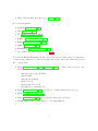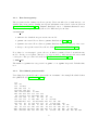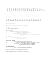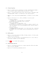
1
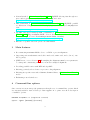
IQPNNI version 3.3 - November 2008
Important Quartet Puzzling and Nearest Neighbor
Interchange
User Manual
Please read carefully before using IQPNNI the first time!
Copyright (C) 2006-2009 by
Bui Quang Minh, Le Sy Vinh, Heiko A. Schmidt,
and Arndt von Haeseler
Copyright (C) 2003-2005 by
Le Sy Vinh and Arndt von Haeseler
Bui Quang Minh
Center for Integrative Bioinformatics Vienna,
Max F. Perutz Laboratories,
Dr. Bohr-Gasse 9/6, A-1030 Vienna, Austria.
email: minh.bui (at) mfpl.ac.at
Heiko A. Schmidt
email: heiko.schmidt (at) mfpl.ac.at
Arndt von Haeseler
email: arndt.von.haeseler (at) mfpl.ac.at
Le Sy Vinh
College of Technology
Vietnam National University of Hanoi
144 Xuan Thuy, Cau Giay, Hanoi, Vietnam
License Agreement
This program is free software; you can redistribute it and/or modify it under the terms of the
GNU General Public License as published by the Free Software Foundation; either version
2 of the License, or (at your option) any later version.
This program is distributed in the hope that it will be useful, but WITHOUT ANY WARRANTY; without even the implied warranty of MERCHANTABILITY or FITNESS FOR
A PARTICULAR PURPOSE. See the GNU General Public License for more details.
Contents
1 Introduction
2
2 Methods
2
3 Main features
3
4 Command-line options
3
4.1
General options . . . . . . . . . . . . . . . . . . . . . . . . . . . . . . . . . . .
5
4.2
IQP options . . . . . . . . . . . . . . . . . . . . . . . . . . . . . . . . . . . . .
6
4.3
Model options . . . . . . . . . . . . . . . . . . . . . . . . . . . . . . . . . . . .
6
4.3.1
Rate heterogeneity . . . . . . . . . . . . . . . . . . . . . . . . . . . . .
8
4.3.2
User-defined protein model . . . . . . . . . . . . . . . . . . . . . . . .
8
Other options . . . . . . . . . . . . . . . . . . . . . . . . . . . . . . . . . . . .
9
4.4
5 Text-menu options
9
5.1
General options . . . . . . . . . . . . . . . . . . . . . . . . . . . . . . . . . . .
10
5.2
IQP options . . . . . . . . . . . . . . . . . . . . . . . . . . . . . . . . . . . . .
10
5.3
Substitution process . . . . . . . . . . . . . . . . . . . . . . . . . . . . . . . .
10
5.4
Rate heterogeneity . . . . . . . . . . . . . . . . . . . . . . . . . . . . . . . . .
12
6 Output files
12
7 Installation
13
7.1
Sequential Version - Binary release . . . . . . . . . . . . . . . . . . . . . . . .
13
7.2
Sequential Version - Source package . . . . . . . . . . . . . . . . . . . . . . .
13
7.3
Parallel Version - Binary release . . . . . . . . . . . . . . . . . . . . . . . . . .
14
7.4
Parallel Version - Source package . . . . . . . . . . . . . . . . . . . . . . . . .
14
8 Version History
15
1
1
Introduction
IQPNNI is a computer program to reconstruct the evolutionary relationships among contemporary species based on DNA, protein, or protein-coding sequences. In case of protein-coding
sequences, several codon models are implemented for inferring positive selection.
IQPNNI is a command-line and menu-driven program which allows users to specify the
parameter values or let the program estimate them from the input data (a nucleotide or
amino acid alignment in PHYLIP format). The options are classified into four main groups,
general options, IQP options, substitution process options, and rate heterogeneity options.
IQPNNI is available free of charge from
http://www.cibiv.at/software/iqpnni/
IQPNNI is written in C++. It will run on most personal computers and workstations if
compiled by a C++ compiler. Please read the Installation section 7 for more details. We
suggest that this documentation should be read before using IQPNNI the first time. To find
out what’s new in the current version please read the Version History section 8.
Important Notice:
In this new version 3.3, IQPNNI supports easier non-parametric bootstrap (see Section
4.1) and fixes some important bugs. Therefore, we strongly recommend you to download
and install this new version.
Since version 3.2, the option “Number of iterations” is changed to “Minimum number of
iterations”, meaning that the program will run at least the specified number of iterations,
no matter if the stopping rule is applied or not. This is to avoid the behavior that IQPNNI
stops so early that does not guarantee to find a good tree. Moreover, another option with
maximum number of iterations is also added, to avoid cases where IQPNNI runs “forever”
since the stopping rule suggest too many number of iterations. For more details see Section
4 and 5.
Since version 3.1, IQPNNI is extended to work on protein-coding sequences. In such cases,
it will first consider the data as DNA and reconstruct a tree based on the HKY85 model.
Then IQPNNI turns the alignment into codon-frames and estimates codon model parameters
based on the reconstructed tree. Finally it infers sites under positive selection using Yang’s
empirical Bayesian method. For more details see Section 8.
2
Methods
To cite the program please use the following papers:
2
• General method: Vinh and von Haeseler (2004) IQPNNI: Moving fast through tree
space and stopping in time, Mol. Biol. Evol. 21(8):1565-1571
http://dx.doi.org/10.1093/molbev/msh176dd
• MPI parallelization: Minh, Vinh, von Haeseler and Schmidt (2005) pIQPNNI - parallel
reconstruction of large maximum likelihood phylogenies. Bioinformatics 21(19):37943796
http://dx.doi.org/10.1093/bioinformatics/bti594
• OpenMP and hybrid MPI/OpenMP parallelization: Minh, Vinh, Schmidt and von
Haeseler (2006) Large maximum likelihood trees. In Proceedings of the 3rd NIC Symposium 2006, pp. 357–365, Forschunungszentrum Jülich, Germany.
http://www.fz-juelich.de/nic-series/volume32/minh.pdf
• Inference of positive selection: please cite this manual.
3
Main features
• Reconstructing maximum likelihood tree on DNA or protein alignment.
• Supporting various substitution models for nucleotide, amino-acid, and codon w/o rate
heterogeneity.
• (NEW in ver. 3.3, see Section 4.1) Resampling the alignment once by non-parametric
bootstrap and constructing an ML tree from the resampled alignment.
• Providing parallel version with MPI and OpenMP.
• Inferring positively selected sites on protein-coding alignment.
• Inferring site-specific rates under Gamma, Gamma+Invar, or Meyer and von Haeseler
model.
• Evaluating a user-defined tree.
4
Command-line options
Since version 3.0, users can specify parameters through a set of command-line options, which
are extremely useful to start a batch job. Run ‘iqpnni -h’ to print out a short description
of available options:
WELCOME TO IQPNNI 3.3 (sequential version)
Syntax: iqpnni [OPTIONS] [Filename]
3
GENERAL OPTIONS:
-h, -?
-n <min_iterations>
-s <stopping_rule>
-u <user_tree>
-bs
-prefix <prefix_out>
-sfc
-ni
print this help dialog
make the main loop to at least min_iterations
either on, off or max <max_iterations>; defaut is off
read the starting tree from user_tree file
construct a bootstrap tree by resampling the alignment
set prefix of output files, default is aln name
start from scratch, don’t load the check point file
don’t prompt for user option
IQP OPTIONS:
-p <probability>
set the probability of deleting a sequence
-k <representatives> set the number of representatives
MODEL OPTIONS:
-m <model>
set the model type for:
Nucleotides: JC69, K2P, F81, HKY85, TN93, GTR
Amino acids: WAG, Dayhoff, JTT, VT, mtREV, rtREV, Blosum
Protein-coding DNA: GY94, YN98, NY98, CP98, CGTR, CPR
Otherwise: Name of file containing user protein model
-w <rate_type>
either uniform, gamma, igamma or sitespec
-c <num_rate>
number of rate categories, for gamma and igamma only
OTHER OPTIONS:
-param <pam_file>
-seed <number>
-wsl
-wpl
-con
use <pam_file> for parameter input (instead of stdin)
set random number generator seed to <number>
write site log-likelihood to .sitelh (PHYLIP-like)
write pattern log-likelihood to .patlh
turn on writing .treels, off by default
You can specify some options first with the command line, and then change again using the
text-menu interface. IQPNNI will start as follows: First, the ‘input file.iqpnni.checkpoint’
file is read if this file is available and the ‘-sfc’ option is NOT specified. If the last run on this
alignment was NOT finished, the parameters recorded in the checkpoint file will be loaded
and all the command line options will be omitted. In this case, you will see some printout
like:
The program was not done from the last run!
Load parameters from the checkpoint file...
IQPNNI now displays the menu and waits for user input if option ‘-ni’ is not specified,
otherwise it starts the computation directly.
4
4.1
General options
-n min iterations and -s stopping rule
These two options are not independent except you specify ‘-s off’. In any case, IQPNNI will
loop at least a number of min iterations. If you set ‘-s on’, the program will automatically
estimate the number of iterations required to ensure that with a 95% confidence, further
search will not detect a better tree. If you set ‘-s max max iterations’, IQPNNI will
always stop after max iterations, even if the stopping rule suggests more iterations. By
‘-s max 0’, it will set max iterations to 10 times of min iterations.
If ‘-n 0’ is specified, IQPNNI will only evaluate ML branch lengths of the starting tree
(either BioNJ tree or user-tree), no topology rearrangement is perform.
-u user tree
Instead of starting the search from BioNJ tree, IQPNNI will make use of the tree from
user tree file in Newick format. The branch lengths of this tree will be ignored, but the
topology will be used to estimate the model parameters and also reestimate the branch
lengths.
-bs
The orginal alignment will be randomly resampled once by non-parametric bootstrap.
The tree will be reconstructed from this resampled alignment. Note that this is NOT a full
bootstrap analysis. You will have to run IQPNNI n times with -bs and -prefix prefix out
(see bellow) to obtain n bootstrap trees. Then, use another program like TREE-PUZZLE
to construct a consensus tree from these n bootstrap trees.
-prefix prefix out
All the output file names will apply this prefix out, instead of using the default alignment
name for the prefix. This option is very handy when combined with -bs to construct several
resampling trees from a bootstrap analysis, so that the output files will not be overwritten.
Following is a small bash script under Linux to do a full bootstrap analysis using IQPNNI
and TREE-PUZZLE (the script should be adapted before real usage):
#! /bin/bash
n=100
filename=alignment.phy
#first, run iqpnni n times
for ((i=1; i<=n; i++)); do
iqpnni $filename -ni -bs -prefix bs-$i
done
#concatenate all resulting trees into a big file
5
cat bs-*.treefile > $filename.bstrees
#now call TREE-PUZZLE to to construct a consensus tree
puzzle -consmrel $filename $filename.bstrees
#NOTE: Choose the option to build a consensus tree from puzzle menu
-sfc
This tells the program not to load the checkpoint file to prevent IQPNNI from recovering
from an interruption.
-ni
This is helpful to start a batch job. The parameters will be displayed again but the program
will not prompt for user input and just start the computation directly.
4.2
IQP options
-p probability and -k representatives
These two options are concerned with the original IQP algorithm, see Vinh and von Haeseler
(2004); Minh et al. (2005) for more details. In short, IQPNNI iterates through a number of
steps to search the tree space. In each step, several taxa are randomly pruned away from
the current best tree. The proportion of deleted leaves is determined by the option ‘-p
probability’. Then these leaves will be reinserted into the tree in a random order following
the IQP algorithm, which takes ‘-k representatives’ parameter into account. This full
tree will be rearranged according to the NNI algorithm, resulting in an intermediate tree. If
this intermediate tree shows a better likelihood, the current best tree will be updated. This
finishes one iteration of the IQPNNI algorithm.
4.3
Model options
-m model
For DNA alignment the following models are implemented:
• JC69 (Jukes and Cantor, 1969).
• K2P (Kimura, 1980).
• F81 (Felsenstein, 1981).
• HKY85 (Hasegawa et al., 1985).
• TN93 (Tamura and Nei, 1993).
6
• GTR - General Time Reversible (e.g., Tavaré, 1986).
For protein alignment:
• Dayhoff (Dayhoff et al., 1978).
• JTT (Jones et al., 1992).
• VT (Müller and Vingron, 2000).
• mtREV (Adachi and Hasegawa, 1996).
• WAG (Whelan and Goldman, 2001).
• rtREV (Dimmic et al., 2002).
• BLOSUM62 (Henikoff and Henikoff, 1992).
• User-defined protein model (see Section 4.3.2).
Note that the BLOSUM62 matrix should better not be used for phylogenetic reconstruction,
because it was constructed for database searches and does not reflect an evolutionary process.
For codon models:
• NY98 (Nielsen and Yang, 1998; Yang et al., 2000): to infer positive selection. Submodels include:
– M0 (One ratio): same as YN98.
– M1 (Neutral).
– M1a (Nearly neutral).
– M2 (Selection).
– M2a (Positive selection).
– M3 (Discrete): default model.
• YN98 (Yang and Nielsen, 1998): special case of NY98 with 1 Ns/Sy category.
• GY94 (Goldman and Yang, 1994).
• CP98 (Pedersen et al., 1998): model incorporating CpG depression.
• CGTR: GTR version of nucleotide for codon (unpublished).
7
4.3.1
Rate heterogeneity
The program can also assume rate heterogeneity. Users can either choose uniform rate over
all sites (rate homogeneity, default), site-specific substitution rates based on the model from
(Meyer and von Haeseler, 2003), Gamma distributed rates, or Gamma+Invariable rates.
Note that rate heterogeneity is only allowed for DNA and protein data.
-w rate type
• uniform: the default homogeneous site rate model.
• gamma: site rates follow a discrete gamma distribution (Yang, 1994).
• igamma: site rates follow a discrete gamma distribution plus one category of zero rate.
• sitespec: site-specific rates follow the model in Meyer and von Haeseler (2003).
Note that for ‘-w sitespec’ option, the tree is first reconstruced based on uniform rate
model. In the second phase, this tree topology is used to infer site-specific rates until
convergence. The procedure is described in Meyer and von Haeseler (2003).
-c num rate
The number of gamma rate categories if ‘-w gamma’ or ‘-w igamma’ is specifed. Default value
is 4.
4.3.2
User-defined protein model
User-defined protein model can be given with ‘-m filename’. An example file which defines
the cpREV model (Adachi et al., 2000) is:
105
227 357
175
43 4435
669 823 538
10
157 1745 768 400
10
499 152 1055 3691
10 3122
665 243 653 431 303 133 379
66 715 1405 331 441 1269 162
145 136 168
10 280
92 148
197 203 113
10 396 286
82
236 4482 2430 412
48 3313 2629
185 125
61
47 159 202 113
68
53
97
22 726
10 145
490
87 173 170 285 323 185
2440 385 2085 590 2331 396 568
1340 314 1393 266 576 241 369
19
40
20
263
21
25
28
691
92
29
66 1745
305 345 218
10 1772 1351
127 454 1268
152 117 219
303 216 516
32 1040 156
8
193
72
302
868
918
327
100
93
645
43
487 1202
148 260 2151
14
56
968
230
323
92
40
754
83
18 435
281 1466
75 592
53
391
54
63
142
200
82
69
42
10 1971
89
91
25 4797
159
189
865
10
247
249
86 468
215 2370
475 317
49
97
122
73
522
167
29
71
760
0.0755 0.0621 0.0410 0.0371 0.0091 0.0382 0.0495 0.0838 0.0246 0.0806
0.1011 0.0504 0.0220 0.0506 0.0431 0.0622 0.0543 0.0181 0.0307 0.0660
The format is following. The first 19 lines describe the bellow triangle of the amino acid
replacement matrix. Then comes a list of 20 amino acid frequencies. The rest of file will be
ignored. The order of amino-acids is:
A
R
N
D
C
Q
E
G
H
I
L
K
M
F
P
S
T
W
Y
V
Ala Arg Asn Asp Cys Gln Glu Gly His Ile Leu Lys Met Phe Pro Ser Thr Trp Tyr Val
4.4
Other options
Other options are easily to understand from the help dialog.
5
Text-menu options
GENERAL OPTIONS
z
Construct a sample tree by bootstrap?
o
Display as outgroup?
n
Minimum number of iterations?
s
Stopping rule?
No
FL-1-103
200
No, stop after 200 iterations
IQP OPTIONS
p
Probability of deleting a sequence? 0.5
k
Number representatives? 4
SUBSTITUTION PROCESS
d
Type of sequence input data?
m
Model of substitution?
t
Ts/Tv ratio (0.5 for JC69)?
f
Base frequencies?
Nucleotides
HKY85 (Hasegawa et al. 1985)
Estimate from data
Estimate from data
RATE HETEROGENEITY
r
Model of rate heterogeneity? Uniform rate
quit [q], confirm [y], or change [menu] settings:
In the following the available options will be briefly introduced.
9
346
10
119
5.1
General options
• Option ‘z’: Switch between reconstructing tree from the orignal alignment (default) or
from a randomly resampled alignment using non-parametric bootstrap.
• Option ‘o’: Users can specify a sequence as the outgroup sequence. The final tree with
the highest likelihood will be rooted with respect to the outgroup sequence.
• Option ‘n’: Users can specify the minimum number of iterations or use the default
value.
• Option ‘s’: Users can choose one of three possibilities to stop the program.
1. The first possibility is
“s Stopping rule? No, stop after ‘n’ iterations”
It means that the program will stop after ‘n’ iterations.
2. The second possibility is
“s Stopping rule (if applicable)? Yes”
It means that the program will stop and output the optimal tree with 95% confidence if at least three better trees found during the search, otherwise it will stop
after ‘n’ iterations.
3. The third possibility is
“s Stopping rule (if applicable)? Yes, and at most ‘max’ iterations”
It is similar to the second possibility, but the program will run at most ‘max’ iterations.
5.2
IQP options
• Option ‘p’: Users can specify the probability of deleting a sequence or let the program
estimate it from the input data.
• Option ‘k’: One can specify number of representatives leaves for a rooted tree. However,
we strongly recommend to use the default value.
See Section 4.2 for more details of these parameters.
5.3
Substitution process
• Option ‘d’: Users must specify the type of sequence input data: Nucleotides, Amino
acids, or Protein-coding DNA.
• Option ‘m’: To switch among substitution models.
10
The subsequent options depend on the type of data and model selected. For DNA models
the following options are available:
• Option ‘f’: Users can specify the base frequencies or let the program estimate them
from the input data.
• Option ‘t’: If HKY85 or TN93 model are chosen, users can specify the transition/transversion
ratio (between 0.2 and 32.0) or let the program estimate it from the input data (default).
• Option ‘u’: For the TN93 model users can also enter the py/pu ratio (the ratio of
pyrimidine transition rate to purine transition rate) between 0.2 and 32.0, or let the
program estimate it from the input data (default).
• Option ‘g’: If users choose GTR model, they can specify six different rate parameters:
1. Transversion rate from A to C,
2. Transition rate from A to G,
3. Transversion rate from A to T,
4. Transversion rate from C to G,
5. Transition rate from C to T,
6. Transversion rate from G to T,
or let the program estimate them from the input data.
For protein models:
• Option ‘f’: Users can specify the amino-acid frequencies from the default frequencies
of the corresponding protein model or let the program estimate them from the input
data.
For codon models:
• Option ‘f’: Users can let the program estimate codon frequencies from the input data
with one of following types: Codon table (default), Equal, F1x4 or F3x4.
• Option ‘t’: Users can specify the transition/transversion ratio (between 0.2 and 32.0)
or let the program estimate it from the input data (default).
• Option ‘w’: If NY98 model is chosen, users can specify the type of submodels (see
Section 4.3).
• Option ‘g’: If NY98 model and ‘Discrete’ submodel are chosen, users can specify the
number of Nonsynonymous/Synonymous classes. Default value is 3.
11
5.4
Rate heterogeneity
• Option ‘r’: To switch among 3 types: Uniform rate, Gamma distributed rate, and site
specific rate.
• Option ‘a’: If users choose Gamma distributed rate, they can specify the Gamma
distribution shape parameter alpha (between 0.1 and 100.0) or let IQPNNI program
estimate it from the input data (default).
• Option ‘c’: If users choose Gamma distributed rates, they can specify a number of
Gamma rate categories between 2 and 32. The default is 4.
• Option ‘i’: To specify the proportion of invariable sites among No (default), Estimate
from data, or a user-defined value.
6
Output files
Running results as well as input parameters are summarized in PREFIX.iqpnni. PREFIX
is by default the input alignment file name. However, if -prefix <prefix out> option is
specified, PREFIX will be assigned with <prefix out>.
Resulting tree will be written to PREFIX.iqpnni.treefile in Newick format.
If Gamma, Gamma+I, or Meyer and von Haeseler’s site-specific model is used, the rates for
each alignment position will be written to PREFIX.iqpnni.rate.
IQPNNI will also create several files:
PREFIX.iqpnni.bionj - BioNJ tree, in Newick format.
PREFIX.iqpnni.treels - List of all intermediate trees, if option -con is specified.
PREFIX.iqpnni.dist - Maximum likelihood distance matrix based on the specified model,
in Phylip format.
PREFIX.iqpnni.sitelh - Site likelihood, if option -wsl is specified.
PREFIX.iqpnni.patlh - Pattern frequency and likelihood, if option -wpl is specified.
PREFIX.iqpnni.checkpoint - program current parameters, will be loaded in case of a crash
or interruption.
PREFIX.iqpnni.prediction - is used internally by the stopping rule. This file is necessary
for recovering from crash or interruption.
PREFIX.iqpnni.bootsample - the bootstrap alignment resampled from the original alignment, if option -bs is specified. This file is also necessary for recovering from crash or
interruption.
12
7
Installation
See below for information how to install/build the different versions of the IQPNNI software.
Executable versions of the sequential, that is, non-parallel program are intended for a number
of operating systems. The parallel program (pIQPNNI) has to be built from the sources, as
it depends on the MPI library locally installed in your system.
7.1
Sequential Version - Binary release
1. You might want to download the executable version of IQPNNI for your operating
system if it is available (iqpnni-XXX-OS.tar.gz or iqpnni-XXX-OS.zip, where XXX is
the current version number and OS the operating system) from
http://www.cibiv.at/software/iqpnni
2. Extract the files (e.g., with tar xvzf iqpnni-XXX-OS.tar.gz under Unix) This should
create a directory iqpnni-XXX.
3. You will find the executable in iqpnni-XXX/src This executable you should rename
to iqpnni (or iqpnni.exe on Windows systems) and copy it to your system’s search
path such that it is found by your system.
If you encounter problems, please ask your local administrator for help.
7.2
Sequential Version - Source package
To build IQPNNI from the sources you need a C++ compiler installed (This is usually the
case on UNIX/Linux systems. For Windows you might want to obtain CygWin/MinWG/MS
Visual C++ or XCode for MacOSX). Then you can follow the procedure below:
1. Download the current version of the software (iqpnni-XXX.tar.gz or iqpnni-XXX.zip,
where XXX is the current version number) from
http://www.cibiv.at/software/iqpnni
2. Extract the files (e.g., with tar xvzf iqpnni-XXX.tar.gz under Unix) This should
create a directory iqpnni-XXX.
3. Change into this directory.
4. To compile the program, type the following:
./configure
This should configure the package for the build. You might also refer to the INSTALL
file for more (general) details.
13
make
This compiles and builds the executable iqpnni (or iqpnni.exe on Windows systems)
to be found in the src directory. This executable can copied to your system’s search
path such that it is found by your system or it can be installed to the default destination
(e.g., /usr/local/bin on UNIX/Linux) using
make install
If you encounter problems, please ask your local administrator for help.
7.3
Parallel Version - Binary release
There will be no binary version of the parallel program because it depends on the MPI
library you have installed locally.
7.4
Parallel Version - Source package
To build the MPI-parallel version of IQPNNI (pIQPNNI) you need a functional C++ compiler installed (This is usually the case on UNIX/Linux systems. For Windows you might
want to obtain CygWin or XCode for MacOSX). In addition you have to install an implementation of the MPI (Message Passing Interface) library. There is a list of (free) implementations at http://www.lammpi.org/mpi/implementations/ available.
Then you can follow the procedure below:
1. Download the current version of the software (iqpnni-XXX.tar.gz or iqpnni-XXX.zip,
where XXX is the current version number) from
http://www.cibiv.at/software/iqpnni
2. Extract the files (e.g., with tar xvzf iqpnni-XXX.tar.gz under Unix) This should
create a directory iqpnni-XXX.
3. Change into this directory.
4. To compile the program, you have to run the configure script with the environment
variable CXX set to the MPI-C++ compiler of your local MPI implementation and
turn on the preprocessor directive PARALLEL, e.g.
env CXX=mpiCC CXXFLAGS="-DPARALLEL -O2" ./configure
This should configure the package for the build using mpiCC as the C++ compiler.
You might also want to refer to the INSTALL file for more (general) details.
14
make
This compiles and builds the executable iqpnni (or iqpnni.exe on Windows systems)
to be found in the src directory. This executable should be renamed to piqpnni and
copied to your system’s search path such that it is found by your system.
5. To run the parallel version please refer to the documentation of your locally installed
MPI implementation and/or ask your local system administrator.
If you encounter problems, please ask your local administrator for help.
8
Version History
Version 3.3
1. Resample the original alignment by bootstrap and construct the tree from the
resampled alignment.
2. By default do not write .treels file. Use ”-con” to turn it on again.
3. Print site and pattern log-likelihood with ”-wsl” and ”-wpl” option.
4. New ”-prefix” and ”-param” options.
5. Code cleanup.
6. Fix some important bugs: incorrect master-worker communication in parallel version (reported by Oliver Mirus), nummerical overflow in stopping rule prediction,
vector overflow in ClusterArr class, and others.
Version 3.2
1. Rewritten user manual.
2. Change “number of iterations” to “minimum number of iterations”.
3. Addtion of maximum number of iterations.
4. GTR model rates are scaled such that the rate from G to T is equal to 1.
5. For G+I model, initialize proportion of invariable sites to the number of constant
sites.
6. Check identical sequences.
Version 3.1
1. Codon model: The program goes through two stages. At first the tree is reconstructed based on HKY model for DNA. Then it applies codon model for inference
of positively selected sites.
2. Gamma + Invariable sites rate heterogeneity.
15
3. Site-specific rates (Meyer and von Haeseler, 2003) improved. Also write out siterates based on empirical bayesian if gamma rate is specified.
4. New protein models: rtREV (Dimmic et al., 2002), user-defined model by a file
containing amino-acid replacement rates and frequencies.
5. Warning if number of iterations is too small as recommended by the stopping rule.
6. New command line options.
7. Bugs fixed:
- Zero state frequencies: they are now replaced by a very small number.
- Checkpoint: now correctly recovered from stopped point.
- Restriction on number of sites: from limit 100,000 to unlimited now.
8. Bugs identified:
- Parallel version on Infiniband system under MPICH.
Version 3.0.1
1. Zero iteration: if user specifies number of iterations to be zero, the program will
only evaluate the starting tree (either BIONJ or user-defined tree) by optimizing
model paramters and branch lengths.
2. Triplet tree: the program can now run on alignment of just 3 sequences.
3. Scaling technique to avoid numerical underflow on large datasets. It now can
stably analyze alignments with more than 1,000 sequences.
4. At least twice faster than v3.0. The ”long double” datatype is replaced by ”double”, making it more compatible to most computers.
5. Memory consumption is reduced at least by half by a new mechanism of storing
conditional likelihood vector.
6. New eigensystem adapted to reversible instantaneous rate matrix.
Version 3.0.beta1
1. The program now runs at least twice faster (applying Newton’s method instead
of Brent’s algorithm and some other algorithmic means).
2. Running in Parallel with Message Passing Interface (MPI).
NOTE The option to change rate heterogeneity is now ‘r’ instead of ‘w’. The stopping
rule is now switched off by default, which can be changed using the ‘s’ option.
Version 2.6
1. General Time Reversible model of evolution.
2. Site-specific substitution rates.
3. Check point: If the program was crashed or stopped by users, it can continue
from the last stopped point.
16
Credits
Some parts of the code were taken from TREE-PUZZLE package (Schmidt et al., 2002). The
source code to construct the BIONJ tree were taken from BIONJ software (Gascuel, 1997).
Acknowledgement
Financial support from the Wiener Wissenschafts-, Forschungs- and Technologiefonds (WWTF)
is greatly appreciated.
References
Adachi, J. and Hasegawa, M. (1996) Model of amino acid substitution in proteins encoded
by mitochondrial DNA. J. Mol. Evol., 42, 459–468.
Adachi, J., Waddell, P. J., Martin, W. and Hasegawa, M. (2000) Plastid genome phylogeny
and a model of amino acid substitution for proteins encoded by chloroplast DNA. J. Mol.
Evol., 50, 348–358.
Dayhoff, M. O., Schwartz, R. M. and Orcutt, B. C. (1978) A model of evolutionary change
in proteins. In Dayhoff, M. O. (ed.), Atlas of Protein Sequence Structure, volume 5, pp.
345–352, National Biomedical Research Foundation, Washington DC.
Dimmic, M. W., Rest, J. S., Mindell, D. P. and Goldstein, R. A. (2002) rtREV: An amino
acid substitution matrix for inference of retrovirus and reverse transcriptase phylogeny. J.
Mol. Evol., 55, 65–73.
Felsenstein, J. (1981) Evolutionary trees from DNA sequences: a maximum likelihood approach. J. Mol. Evol., 17, 368–376.
Gascuel, O. (1997) BIONJ: An improved version of the NJ algorithm based on a simple
model of sequence data. Mol. Biol. Evol., 14, 685–695.
Goldman, N. and Yang, Z. (1994) A codon–based model of nucleotide substitution for
protein–coding DNA sequences. Mol. Biol. Evol., 11, 725–736.
Hasegawa, M., Kishino, H. and Yano, T.-A. (1985) Dating of the human–ape splitting by a
molecular clock of mitochondrial DNA. J. Mol. Evol., 22, 160–174.
Henikoff, S. and Henikoff, J. G. (1992) Amino acid substitution matrices from protein blocks.
Proc. Natl. Acad. Sci. USA, 89, 10915–10919.
Jones, D. T., Taylor, W. R. and Thornton, J. M. (1992) The rapid generation of mutation
data matrices from protein sequences. Comput. Appl. Biosci., 8, 275–282.
17
Jukes, T. H. and Cantor, C. R. (1969) Evolution of protein molecules. In Munro, H. N. (ed.),
Mammalian Protein Metabolism, volume 3, pp. 21–123, Academic Press, New York.
Kimura, M. (1980) A simple method for estimating evolutionary rates of base substitutions
through comparative studies of nucleotide sequences. J. Mol. Evol., 16, 111–120.
Meyer, S. and von Haeseler, A. (2003) Identifying site-specific substitution rates. Mol. Biol.
Evol., 20, 182–189.
Minh, B. Q., Vinh, L. S., von Haeseler, A. and Schmidt, H. A. (2005) pIQPNNI – parallel
reconstruction of large maximum likelihood phylogenies. Bioinformatics, 21, 3794–3796.
Minh, B. Q., Vinh, L. S., Schmidt, H. A. and von Haeseler, A. (2006) Large maximum
likelihood trees. In Proceedings of the 3rd NIC Symposium 2006, pp. 357–365, Forschunungszentrum Jülich, Germany.
Müller, T. and Vingron, M. (2000) Modeling amino acid replacement. J. Comput. Biol., 7,
761–776.
Nielsen, R. and Yang, Z. (1998) Likelihood models for detecting positively selected amino
acid sites and applications to the HIV-1 envelope gene. Genetics, 148, 929–936.
Pedersen, A. K., Wiuf, C. and Christiansen, F. B. (1998) A codon-based model designed to
describe lentiviral evolution. Mol. Biol. Evol., 15, 1069–1081.
Schmidt, H. A., Strimmer, K., Vingron, M. and von Haeseler, A. (2002) TREE-PUZZLE:
Maximum likelihood phylogenetic analysis using quartets and parallel computing. Bioinformatics, 18, 502–504.
Tamura, K. and Nei, M. (1993) Estimation of the number of nucleotide substitutions in the
control region of mitochondrial DNA in humans and chimpanzees. Mol. Biol. Evol., 10,
512–526.
Tavaré, S. (1986) Some probabilistic and statistical problems on the analysis of DNA sequences. Lec. Math. Life Sci., 17, 57–86.
Vinh, L. S. and von Haeseler, A. (2004) IQPNNI: Moving fast through tree space and stopping in time. Mol. Biol. Evol., 21, 1565–1571.
Whelan, S. and Goldman, N. (2001) A general empirical model of protein evolution derived
from multiple protein families using a maximum likelihood approach. Mol. Biol. Evol., 18,
691–699.
Yang, Z. (1994) Maximum likelihood phylogenetic estimation from DNA sequences with
variable rates over sites: Approximative methods. J. Mol. Evol., 39, 306–314.
Yang, Z. and Nielsen, R. (1998) Synonymous and nonsynonymous rate variation in nuclear
genes of mammals. J. Mol. Evol., 46, 409–418.
Yang, Z., Nielsen, R., Goldman, N. and Pedersen, A.-M. K. (2000) Codon-substitution
models for heterogeneous selection pressure at amino acid sites. Genetics, 155, 431–449.
18