Download User Manual

CGH-Plotter
User Manual
Contents
1 Introduction
2
2 Installation
2.1 Installation Instructions . . . . . . . . . . . . . . . . . . . . .
2
2
3 Instructions
3.1 User Interface Pages . . .
3.1.1 Main Page . . . . .
3.1.2 Create Data Struct
3.1.3 Find Amplicons . .
3.1.4 BP Filter . . . . .
3.1.5 BP Convert . . . .
3.1.6 Plot Data . . . . .
3.1.7 Write TXT . . . .
.
.
.
.
.
.
.
.
.
.
.
.
.
.
.
.
4 Methods
4.1 Filtering . . . . . . . . . . . .
4.2 k -means Clustering . . . . . .
4.3 Dynamic Programming . . . .
4.4 Filtering according to basepair
5 Summary
.
.
.
.
.
.
.
.
.
.
.
.
.
.
.
.
.
.
.
.
.
.
.
.
.
.
.
.
.
.
.
.
. . . .
. . . .
. . . .
units
.
.
.
.
.
.
.
.
.
.
.
.
.
.
.
.
.
.
.
.
.
.
.
.
.
.
.
.
.
.
.
.
.
.
.
.
.
.
.
.
.
.
.
.
.
.
.
.
.
.
.
.
.
.
.
.
.
.
.
.
.
.
.
.
.
.
.
.
.
.
.
.
.
.
.
.
.
.
.
.
.
.
.
.
.
.
.
.
.
.
.
.
.
.
.
.
.
.
.
.
.
.
.
.
.
.
.
.
.
.
.
.
.
.
.
.
.
.
.
.
.
.
.
.
.
.
.
.
.
.
.
.
.
.
.
.
.
.
.
.
.
.
.
.
.
.
.
.
.
.
.
.
.
.
.
.
.
.
.
.
.
.
.
.
4
4
4
6
10
12
16
19
29
.
.
.
.
31
31
34
35
36
37
1
1
Introduction
Copy number changes, such as deletions and amplifications, are common
aberrations in cancer and are known to involve genes that play a crucial role
in the development and progression of the malignant disease [5]. The copy
number changes span usually large regions of the genome and therefore influence multiple genes at the same time. Comparative genomic hybridization
(CGH) on DNA microarray allows simultaneous monitoring of copy numbers
of thousands of genes throughout the genome [6], [7].
CGH-Plotter is a versatile software that allows the user to plot CGH
copy number data as a function of the position of the genes along the human genome, and to rapidly determine the exact locations of copy number
changes, such as amplicons and deletions.
In this user manual we explain in details:
1. How to install CGH-Plotter,
2. How to use CGH-Plotter,
3. How to store and analyze the results,
4. What are the assumptions behind the analysis.
We also provide several examples on the use of CGH-Plotter.
2
Installation
CGH-Plotter requires Matlab 6.1 or higher in order to operate. Accordingly,
all data must be in Matlab (*.mat) format or in tab delimited text (*.txt)
format.
2.1
Installation Instructions
Archive ’CGH-Plotter.zip’ consists of five folders: CGH-Plotter, gui, ampli math, data structs and ampli data.
• Main folder CGH-Plotter contains the following folders and files:
– gui
2
– ampli math
– ’CGH Plotter.m’ and ’CGH Plotter.fig’.
• Folder gui (Graphical User Interface) includes functions and corresponding figures:
–
–
–
–
–
–
–
’create struct.m’, ’create struct.fig’
’amplikoni.m’, ’amplikoni.fig’
’bp filter.m’, ’bp filter.fig’
’bp convert.m’, ’bp convert.fig’
’plot data.m’, ’plot data.fig’
’write txt.m’, ’write txt.fig’
’end all.m’, ’end all.fig’
• Folder ampli math includes all mathematical functions used in CGHPlotter:
–
–
–
–
–
–
–
–
–
–
–
–
’bp median.m’
’combined.m’
’compute kmean.m’
’cumulative.m’
’define amplicons.m’
’dynamic prog.m’
’filter data.m’
’find regions’
’handle NaNs.m’
’kmean.m’
’transform data.m’
’writeresults.m’
• Folder data structs can be located arbitrary. It is meant for storage of
data structs of CGH-data and is initially empty.
• Folder ampli data is intended for storing the analyzed data and it can
be located arbitrary. Folder ampli data is initially empty.
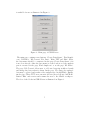
The diagram of folders in CGH-Plotter is illustrated in Figure 1.
3
.../CGH-Plotter
/gui
/ampli_math
/data_structs
/ampli_data
Figure 1: Folders of CGH-Plotter. Folders gui and ampli math are subfolders
of CGH-Plotter, data structs and ampli data can be located arbitrary.
3
Instructions
Basically CGH-Plotter functions as follows. First, CGH-Plotter filters the
data using median or mean filter with window size that has been input. Secondly, the filtered data are clustered using the k -means clustering algorithm.
The purpose of the k -means clustering is to find the maximum number of
amplicons/deletions at each chromosome. This number is required by the
last phase, dynamic programming, which actually estimates the amplicons
and deletions. CGH-Plotter saves the result file, which consists of the original data, filtered data, probable amplicons and deletions, indices to the
changes of amplicons and deletions of the CGH-data, names of the samples,
cumulative basepairs and genomic indices.
To be more precise, CGH-Plotter consists of five phases:
1. CGH-Plotter creates a data struct of separate data files that the user
has specified,
2. CGH-Plotter reads the data struct,
3. CGH-Plotter analyzes the data struct,
4. CGH-Plotter stores the analyzed data,
5. CGH-Plotter plots the data.
In this section a more detailed explanation is given for each of these phases.
3.1
3.1.1
User Interface Pages
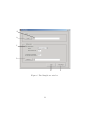
Main Page
CGH-Plotter is started with command ’CGH Plotter’, providing that current
directory in Matlab is CGH-Plotter. Main page is opened and CGH-Plotter
4
is available for use as illustrated in Figure 2.
Figure 2: Main page of CGH-Plotter.
The main page contains seven buttons: ’Create Data Struct’, ’Find Amplicons’, ’BP Filter’, ’BP Convert’,’Plot Data’, ’Write TXT’ and ’Exit’. First,
the data struct should be constructed in the page ’Create Data Struct’, if it
is not done already. After the data struct is created and stored, the analysis
part is executed at the page ’Find Amplicons’ or at the page ’BP Filter’.
The page ’BP Convert’ allows user to add new basepairs in filtered result
and interpolate data values for them. In the page ’Plot Data’ the analyzed
data may be plotted and results of the analysis saved in ASCII file. Finally,
int the page ’Write TXT’ user can write all data (if needed) into ASCII file.
Button ’Exit’ ends session and returns the user to the Matlab workspace.
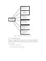
The idea of the blocks in CGH-Plotter is illustrated in Figure 3.
5
Create Struct
- creates data struct
- saves data struct
Find Amplicons
- loads data struct
- analyzes data
- stores results
BP Filter
- loads data struct
- analyzes data
- stores results
CGH-Plotter
(main page)
BP Convert
- adds new basepairs
- interpolates NaNs
Plot Data
- loads analyzed data
- plots data
- saves results of analysis
in ASCII file
Write TXT
- loads analyzed data
- saves data to text file
according to users
selections
Figure 3: Main tasks of CGH-Plotter blocks.
3.1.2
Create Data Struct
In the page ’Create Data Struct’ one is able to create a data struct that
consists of the CGH-data and essential indices. It is assumed throughout
CGH-Plotter that the data contain fields given in this section. All the data
has to be either
1. in Matlab (*.mat) format or
2. in tab delimited text (*.txt) format.
6
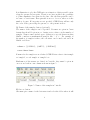
Examples of the files (both formats) are in folder \CGH−P lotter\data structs.
A
B
C
D
E
F
G
Figure 4: Create Data Struct -window.
A) Data-button (obligatory)
This button enables loading of the data file. The data file is assumed to be
m × n matrix, where m is the number of genes and n is the number of the
samples. Furthermore, it is assumed that the genes are arranged according
to their genomic order from p-telomere of chromosome 1 to q-telomere of the
Y chromosome. This order of genes is referred to as genomic index. Missing
values have to be replaced with NaNs (Not-a-Numbers). Finally, the data
should not be transformed e.g. with log-transform prior to CGH-Plotter.
After selecting a data matrix, the name of the selected data appears to the
text box next to data button.
B) Chromosome indices -button (obligatory)
7
As it is essential to know where each chromosome begins, the starting points
of the chromosomes as indices to the data matrix needs to be specified. Chromosome indices is a 24 × 1 matrix. First 22 indices are the starting points of
chromosomes 1-22, 23:rd is the starting point of chromosome X and 24:th of
the chromosome Y. Also the chromosome indices can be in *.txt or in *.mat
format. An example of chromosome indices matrix in *.mat format is shown
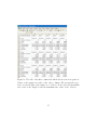
below: [3]
⎡
⎢
⎢
⎢
⎢
⎢
⎢
⎢
⎢
⎢
⎢
⎢
⎢
⎢
⎢
⎢
⎢
⎢
⎢
⎢
⎢
⎢
⎢
⎢
⎢
⎢
⎢
Chromosome indices = ⎢
⎢
⎢
⎢
⎢
⎢
⎢
⎢
⎢
⎢
⎢
⎢
⎢
⎢
⎢
⎢
⎢
⎢
⎢
⎢
⎢
⎢
⎢
⎢
⎢
⎢
⎣
1
1338
2121
2829
3292
3851
4548
5115
5480
5924
6408
7047
7729
7941
8353
8701
9193
9812
9994
10695
11047
11198
11529
11980
⎤
⎥
⎥
⎥
⎥
⎥
⎥
⎥
⎥
⎥
⎥
⎥
⎥
⎥
⎥
⎥
⎥
⎥
⎥
⎥
⎥
⎥
⎥
⎥
⎥
⎥
⎥
⎥
⎥
⎥
⎥
⎥
⎥
⎥
⎥
⎥
⎥
⎥
⎥
⎥
⎥
⎥
⎥
⎥
⎥
⎥
⎥
⎥
⎥
⎥
⎥
⎥
⎥
⎦
CGH-Plotter adds the last index of the chromosome ’Y’ to chromosome indices matrix. Therefore the chromosome indices is a 25 × 1 matrix during
the analysis.
C) Base-pairs -button (optional)
8
It is illustrative to plot the CGH ratios as a function of their actual location
along the genome in base-pairs. Therefore we have included the possibility
to define cumulative base-pairs for the data. Also the Base-pairs file can be
in *.mat or *.txt format. Base-pairs file is an m × 1 vector, where m is the
number of genes. If base-pairs are not specified, CGH-Plotter will use only
the order of the genes along the genome, i.e. the genomic indices.
D) Names of the samples -button (optional)
The names of the samples can be specified. If names are given in *.mat
format they should be given in n × 1 string vector, where n is the number of
samples. Names cannot include space characters or special characters that
Matlab considers as mathematical symbols, like ’-’ or ’+’. For example, if
the number of samples is three, the cell struct can be made and saved in
Matlab as follows.
>>Names = [{’BT474’}; {’MCF7’}; {’ZR7530’}]
>>save Names Names
If names for the samples are not defined, CGH-Plotter refers to first sample
as ’sample1’, second sample as ’sample2’ etc.
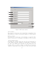
Furthermore if the names are defined in *.txt file, they must be given in
one row and each in own column as shown in figure 5.
Figure 5: Names of the samples in *.txt file.
E) Save as -button
One must give a name for the data struct and select the folder where it will
9
be saved. Folder data structs is meant for this purpose, but it is not obligatory to save data structs there.
F) Create -button
CGH-Plotter creates a data struct. When the struct is created a message
box with text ’Ready’ pops out.
G) Main page -button
Main page -button returns one to the main page.
Data struct can also be created manually. However, the struct must have
the following fields:
• data struct.data (CGH-data, size m × n ),
• data struct.chromo (Indices to chromosomes, size 25 × 1),
• data struct.basepair (Cumulative base-pairs, size m × 1),
• data struct.samples (Names of the samples, size n × 1).
3.1.3
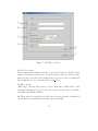
Find Amplicons
Phase ’Find Amplicons’ involves several components. The aim of this phase
is first to find amplicons or deletions and then create a result file for plotting.
A) Load data -button
This button enables loading of the data struct made in phase ’Create Data
Struct’.
B) Selected data -text box
When the data have been selected, the name of the data file can be seen in
the text box next to ’Load data’ button.
C) Filter parameters
• It is possible to specify the type of the filter, possible options are ’Move
median’ and ’Move average’. By default CGH-Plotter uses ’Move median’ filter.
10
B
A
C
D
E
Figure 6: Find Amplicons -window.
11
F
• Also the window size for filtering the data may be defined. Default
window size is five. Window size is dependent on the amount of noise
in the data. When the amount of the noise in the data is small, it is
enough to have small window size (e.g. 1-3). However, if data are very
noisy, window size should also be quite large (> 5).
D) Constant for computing the number of changes.
One may specify the constant that is used when the number of changes is
computed. Default constant is six. The procedure how to compute the number of the changes along with some guidelines is given in Section 4.2.
E) Save As -button
Before starting the analysis, one has to specify the name for the data struct
to be analyzed. Save As -button opens a Save As -dialog and the name and
the location for the result file may be selected. It is recommended that result
files are stored in the folder ampli data.
F) Start -button
After providing all required information the analysis may be started by selecting the ’Start’ button. Analysis of the data takes few minutes. For example,
analysis of CGH ratios of 11994 genes from 14 samples with Intel Pentium
IIII/2.4 GHz took approximately 5 minutes. When CGH-Plotter is ready, a
message box appears notifying that the data set has been successfully analyzed and results of the analysis are saved.
G) Main Page -button
By pushing ’Main Page’ button one can return to the main page.
3.1.4
BP Filter
In ’BP Filter’ phase it is possible to filter data with filters that have constant
window length in basepairs. It is also possible to ignore filtering certain areas
in data by specifying only special regions to be filtered. These regions are
given in separate input file.
A) Load -button
This button enables loading of the data struct made in phase ’Create Data
Struct’.
12
A
B
C
D
E
F
Figure 7: BP Filter -window.
B) Save As -button
Before starting the analysis, user has to specify the name for the file where
analyzed data will be saved. Save As -button opens a Save As -dialog and the
name and the location for the result file may be selected. It is recommended
that result files are stored in the folder ampli data.
C) Filter options
’Filter type’ selection allows user to decide, what kind of filter will be used
during the filtering process. For now only options for filter type are BP Median filter and BP Mean Filter.
In ’Filter window length (in bps)’ field user can specify window length for
chosen filter in basepair units. Default option is 500000.
13
D) Optional region info
Optional region info can be loaded by pressing Load -button in this section.
With this info user can ignore gaps like centromere and telomere regions.
Data values outside these regions will have no effect on the filtering result.
Startpoints
Endpoints
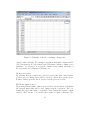
Figure 8: Example of the region info file
Region info file must be either in matlab (*.mat) or in tab delimited text
(*.txt) format. If *.mat format is used, then file must contain variable that
is Nx2 matrix containing start point and end point (in cumulative basepair
units) for every N separate regions. Element (i,1) of the matrix is considered
as a start point for i’th region and element (i,2) as an end point for i’th region. Name of the variable in *.mat the file must equal to filename. If *.txt
format is used, file must contain a matrix (similar to one described above)
in tab delimited text format. Structure of the region info file is illustrated in
figure 8.
14
If user does not load any special region info, chromosome limits included
in data struct will be considered as start points and end points for regions.
(This means that each chromosome is filtered separately but other known
gaps in data will not be ignored.)
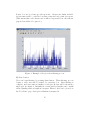
Figure 9: Example of the plot after filtering process
E) Start -button
User can begin filtering by pressing Start-button. When filtering process
begins or ends, user will be notified by a message box. After filtering is
complete, used true window lengths for each gene in data will be shown in a
single plot (see figure 9. Information on true window lengths can be useful
when adjusting window length in basepairs. Filtered data can be plotted at
the ’Plot Data’ page. Such plot is illustrated in figure 10.
15
Figure 10: Example of the plotted BP filtered result
F) Main Page -button
The Main Page -button takes user back to the main page.
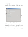
3.1.5
BP Convert
In ’BP convert’ phase it is possible to manipulate basepairs in filtered data
file. Basepair info in the file can be replaced with a new basepair structure
given as a separate input. If the new basepairs contain such pairs that are
not present in original data file, CGH and filtered data values for those pairs
will be NaNs. These (and all other) NaNs can have an interpolated data
value if interpolation window is specified.
Interpolation process can be adjusted by giving as a separate input those
regions (in cumulative basepair units) where interpolation is needed. Also
maximum length for interpolation window can be specified.
16
A
B
C
D
E
F
G
H
Figure 11: BP Convert -window.
A) Load -button
By pressing Load -button user can load data file that contains filtered data.
(Data must have been filtered in either Find Amplicons or BP filter phase.)
B) Save as -button
By pressing Save as -button user can select filename for output file. If filename is correctly selected, it will appear on the right side of Save as -button.
C) New basepairs -button
By pressing New basepairs -button user can select new basepair info for
loaded datafile (see A). File containing new basepairs must be in either matlab *.mat or tab delimited text *.txt format. If *.mat format is used, the
file must contain a one variable (column vector) that lists new basepairs in
cumulative basepair units and in ascending order. Name of the variable must
17
Figure 12: Example of the file containing basepair info
equal to name of the file. For example basepairtest.mat must contain variable
called basepairtest. If *.txt format is used, file must contain a column vector
(similar to one described above) in tab delimited text format. Structure of
the region info file is illustrated in Figure 12.
D) Regions -button
By pressing Regions -button user can select region info that controls interpolation process. Interpolation will be executed only in these given regions.
Format of this region info file is described in the previous section.
E) Chromo limits -button
By pressing Chromo limits -button user can select general chromosome limits
(in basepair units) that will be used during basepair conversion. File containing the region info must be in matlab *.mat format and it must contain
variable called chromo or a variable whose name is equal to filename. The
18
variable must be 25x1 vector containing start points for every chromosome
and an end point for last chromosome (in 25’th element).
F) Interpolate gaps shorter...
In this field user can specify the longest gap (in basepair units) that will be
interpolated. If there are less than two clones in that area, interpolation will
not be done. Default value for this field is 150000 BPs.
G) Start -button
By pressing start button user can start the conversion process. Status of the
process will be show in a message box.
H) Main page -button
The Main Page -button takes user back to the main page.
3.1.6
Plot Data
In ’Plot Data’ phase it is possible to compare the data and results from
dynamic programming. One may choose the properties of the created data
set to be illustrated. It is possible to plot the CGH-data as ratios or logtransformed ratios, and to plot amplicon boundaries from an individual sample or combined amplicon boundaries from a group of samples.
One may plot the CGH-data, filtered data, or amplicon boundaries either from one chromosome or across all chromosomes. It is also possible to
plot results from several samples at the same time. Thus one may choose
whether the results are illustrated in one figure or in multiple figures. By
default CGH-Plotter uses genomic indices to plot the data but one may also
select to use cumulative basepairs.
A) Choose data -button
By pushing choose data -button one can select the data to be illustrated.
Result file has to be constructed in the ’Find Amplicons’ phase, and consist
of seven fields:
• ’data’: CGH-data,
• ’datafilt’: Filtered data,
19
• ’dp’: Amplicon boundaries computed with dynamic programming,
• ’tu’: Indices to the changes of amplicon boundaries,
• ’chromo’: Indices to chromosome starts,
• ’basepair’: Cumulative base-pairs,
• ’samples’: Names of the samples.
Only one data set can be illustrated at a time but it is possible to observe
several properties of the data simultaneously.
B) Selected data -text box
The name of the selected data file is seen in textbox: ’Selected data’.
F
G
H
B
A
C
D
E
K
I
L
M
J
O
N
Figure 13: Plot Data -window.
20
P
C) Data type
The CGH-data can be plotted either as log-transformed or as ratios. If the
the data is plotted as log-transformed, CGH-Plotter adds ’1’ to the natural
logarithm value in order to move the baseline to around ratio of one. In every
case amplicon/deletion boundaries and filtered data are seen as ratios.
D) Samples
One may choose which CGH-data sample he wants to plot. If the last option
’All’ is selected, CGH-Plotter adds the selected chromosome of each sample
to the data listbox.
E) Chromosome
In CGH-Plotter one needs to select either the chromosome that he wants to
illustrate or the option ’All’ when the ratios of the sample will be plotted
genome-wide.
F) Add -button
After above mentioned attributes are selected ’Add -button’ will take the
facts of the data to the listbox on the right. Data must always be exported
to the data listbox, because CGH-Plotter handles only the data in listbox.
G) Data listbox
In the data listbox one can see the part or parts of the data that
CGH-Plotter is about to plot. Parts of the data are written in the form:
’Data name: Data type, Sample, Chromosome’. It is possible to select several parts of the data, but the number of genes must be same for every part.
H) Remove -button
’Remove’ button removes selected data from the data listbox. First one has
to select the data that is wanted to be removed.
I) Plot
One can select the properties to be plotted.
• If ’Data’ is selected, CGH-Plotter plots original CGH-data.
• If ’Amplicon boundaries’ is selected, CGH-Plotter will plot the amplicon/deletion boundaries that are computed by the dynamic programming algorithm.
21
• If ’Combined amplicon boundaries’ is selected, CGH-Plotter will plot
combined amplicon boundaries from selected samples.
• The method for computing the combined amplicon boundaries can be
selected. Possible choices are average, median, maximum, and minimum. By default CGH-Plotter uses average.
• If ’Filtered Data’ is selected, CGH-Plotter will plot filtered data that
are computed by the filtering algorithm. The window size and the type
of the filter were determined in the phase ’Find Amplicons’.
J) Show results
One can select how he wants CGH-Plotter to present the data.
• If ’superimpose all data to one figure’ is selected CGH-Plotter will
plot all selected data to the same figure. Each sample, filtered data
of the sample and amplicon boundaries of the sample have the same
color, samples are illustrated with points, filtered data and amplicon
boundaries with lines. Combined amplicon boundaries are seen as thick
black line (Figure 14).
• If one selects ’each plot to own figure’, CGH-Plotter will illustrate every
sample individually (Figures 15 and 17). CGH-Plotter plots CGH-data
with blue line and amplicon boundaries with red. If ’Filtered data’ is
selected CGH-Plotter will plot filtered data of the sample with green
line and if ’Combined amplicon boundaries’ is selected CGH-Plotter
will plot combined boundaries with black line.
K) Index to a gene
One may select whether he wants to see cumulative base-pairs in the x-axis
instead of genomic indices.
L) Baseline
One may select whether he wants CGH-Plotter to use median of each chromosome as baseline of the chromosome. By default baseline is value ’1’.
M) One may select to define adjoining amplicons (or deletions) as one amplicon (deletion) in the resulted boundary-file.
N) Save Boundaries -button
22
This button allows one to specify a name for the boundary file and select the
folder where he wants to save it. CGH-Plotter creates a tabular separated
ASCII file as illustrated in figure 19. If the name is not specified, the results
are not saved. By default CGH-Plotter will save the amplicons with height
over 1.2 and deletions with height smaller than 0.95. If needed it is really
straightforward to change these limits in the beginning of the function DefineAmplicons.m. If the file where to one is about to save the results already
exists CGH-Plotter will write the results after the existing text.
O) Plot -button
CGH-Plotter plots only the data that are seen in the data -list box and uses
properties that have been specified. CGH-Plotter shows a message box that
gives genomic indices to the amplicons. (Name of the samples: indices of the
boundaries). Amplicon boundaries -message is modal and it will disappear
permanently after pushing the OK-button.
P) Main Page -button
’Main Page’ button takes one back to the main page.
A capture of the typical plotting figure is provided in Figure 14, which illustrates the ratios from chromosome 20 across five samples. It is also possible
to explore only one of the samples by illustrating it separately as shown in
Figure 15. Amplicon/deletion boundaries of the samples are listed in Figure 18, while Figure 19 illustrates the created ASCII file that reveals the
properties of each amplicon and deletion.
23
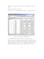
Chr 20
SKBR3
MCF7
BT474
BT20
MDA361
8
7
6
5
4
3
2
1
3.02
3.03
3.04
3.05
3.06
3.07
9
x 10
Figure 14: Ratios from five samples (chromosome 20) illustrated in one figure. Amplicon boundaries are seen with the same color as the corresponding
sample. Combined amplicon boundaries are colored black. Cumulative basepairs are in the x-axis.
24
BT474 chr 20
4
3.5
3
2.5
2
1.5
1
0.5
1.07
1.075
1.08
1.085
1.09
1.095
1.1
4
x 10
Figure 15: Chromosome 20 of the sample ’BT474’. CGH-Plotter has now
plotted each of selected data into different figures using genomic index. CGHdata is blue line, amplicon boundaries red line. NaN values of original data
are now marked with crosses. Underneath of the data is a bar where the
amplicons and deletions of the data are marked with red and green bars.
HCC1428 chr 20
3
2.5
2
1.5
1
0.5
3.02
3.03
3.04
3.05
3.06
3.07
9
x 10
Figure 16: Chromosome 20 of sample HCC1428 plotted against cumulative
basepairs. CGH-data are seen in blue, and filtered data as green line.
25
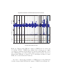
SKBR3 chr All
8
7
6
5
4
3
2
1
1
2
3
4
5
6
7
8 9
10 11
12
1314 15 16 17
18
19
20 21
22 X
Y
Figure 17: All chromosomes of sample SKBR3. CGH-data are seen in blue,
and amplicon boundaries as red line. CGH-Plotter plots dividing lines between the chromosomes. The bar below the data is indicating the amplicons
and deletions.
Figure 18: Amplicon Boundaries message box.
26
Figure 19: The title of the first column tells which chromosome is in question.
Names of the samples are titles of the other columns. File presents the type,
start, end and height of the amplicon or deletion. It also gives the maximum
ratio value of the amplicon and the minimum ratio value of the deletion.
27
Copy Number Alterations in the BT474 Breast Cancer Cell Line Genome
CGH-Plotter:
Original data
1.5
1.5
1
Chromosomal
CGH
CGH-Plotter:
Amplicon/deletion boundaries
1
1
2
3
500000000
4
5
1000000000
6
7
8
1500000000
9
10
11
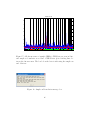
12
2000000000
13
14
15 16
17
2500000000
18
19 20 21 22
X
3000000000
Cumulative Genomic Base Pair Location
Figure 20: Chromosomal CGH and output of CGH-Plotter for breast cancer cell line ’BT474’. CGH-Plotter original data is shown on top, amplicon/deletion boundaries in the middle and chromosomal CGH-data on bottom. CGH-Plotter can clearly identify amplicons and deletions detected by
chromosomal CGH and, as expected due to the higher resolution of arrayCGH, also reveals additional aberrations.
In order to compare the performance of CGH-Plotter we have illustrated
both the chromosomal CGH and the output of CGH-Plotter in Figure 20.
28
3.1.7
Write TXT
In phase ’Write TXT’ user can write analyzed data (or simply contents of
data struct) to text file for further analysis. Data will be printed in tab delimited text format.
A
B
C
D
E
F
Figure 21: BP Filter -window.
A) Choose data -button
By pressing Choose data -button user can select analyzed data or a data
structure that will be converted to text file. If selected file is not in correct
format, other options in the window will not be enabled. If file is in correct
format, its name will appear on the right side of Choose data -button.
B) Save as -button
By pressing Save as -button user can select filename for output text file. If
29
filename is correctly selected, it will appear on the right side of Save as button.
C) Sample and Chromosome options
User can choose one or all samples/chromosomes to be printed in text file.
Figure 22: Example of resulting txt file
D) CGH Data, Filtered Data, DP Data and other Checkboxes
User can choose any combination of active checkboxes in this section. If
checkbox is selected, corresponding data is going to be printed into text file.
If none of the checkboxes is selected, only basepair and chromosome information will be printed. If one or several of checkboxes are in inactive state,
it indicates that loaded data file does not contain that type of data.
30
If Write interpolation info -checkbox is selected, 0 or 1 will be printed after every filtered data value in output file. 1 indicates that the data value is
interpolated, whereas 0 indicates that the data value is not interpolated.
If Write BP filter window size -checkbox is selected, true window sizes (that
were used in filtering) will be printed for each clone index.
E) Write -button
Writing to text file begins when Write-button is pressed. When writing process begins or ends, user will be notified by a message box. Resulting text
file is illustrated in figure 22.
F) Main Page -button
Main Page -button takes user back to main page.
4
Methods
In this section we describe the methods used in CGH-Plotter in greater detail.
The overall view for CGH-Plotter is given in Figure 23.
4.1
Filtering
Before applying the k -means clustering, CGH-ratios in each chromosome are
filtered with the moving median or average filter. The user may input the
type (i.e. mean or median) and the size of window for the filter. Suggested
window sizes are between three and nine.
The filtering proceeds as follows. First CGH-Plotter computes the median/average of first w values, where w is the size of the window. For example, if w is five, the first value in the filtered data is median/average of
the first five CGH-data points. Then CGH-Plotter takes again w values
beginning from the second data point and computes the median/average depending on the user’s choice. The filtering stops when the last data point
is reached. Therefore, in standard filtering utilizing moving window, the filtered data are w -1 shorter than the original data. In order to keep data sets
31
in the same size as the originals, CGH-Plotter inputs w -1 NaNs at the end
of each chromosome. The chromosomes are filtered individually because, for
example, otherwise values in the end of chromosome one would affect to the
values of the chromosome two. [1] The filtered data are saved and so it is
possible to plot filtered data in the phase ’Plot data’.
32
User inputs
CGH-Plotter
Data
Chromosome indices
Basepairs
Names
Create Struct
Struct
Struct
Find Amplicons
BP filtering
Find number of changes
Median/Average filter
Window size
Change function
k-means
Filtering
-define the num-median/average clustering
ber of changes
-clusters the
-window size
data to three
clusters
Filtered data
Clustered data Number of changes
Dynamic
Programming
Filtering
-median filter
-constant window size in basepair units
-filters only outside known gaps
Constant for
computing DC-levels
Window size
Known gaps
Analyzed
data
Analyzed
data
Analyzed
data
BP convert
Conversion to new basepairs
-interpolates missing values
-interpolates only outside known gaps
New basepairs
Known gaps
Analyzed
&
Interpolated
data
Plot Data / Write TXT
Figures
ASCII file
Figure 23: Overall view of CGH-Plotter. The user inputs CGH-data, chromosome indices, basepairs and names of the samples in ’Create Struct’ phase.
CGH-Plotter creates a struct that is used in the phase ’Find Amplicons’. Further, the user defines the type of the filter and size of the window, which are
used in filtering phase. CGH-Plotter clusters filtered data into three clusters
with k -means clustering algorithm. Clustered data are delivered to the function that computes the maximum number of the change points. The number
of changes is needed when dynamic programming algorithm computes the
amplicons and deletions. In ’Plot Data’ and ’Write TXT’ phase the user
may plot the results of the analysis and save the results in ASCII-file.
33
Analyzed
data
4.2
k -means Clustering
k -means clustering algorithm is used for finding the number of amplicons/
deletions for each chromosome. The idea behind the k -means clustering is to
cluster the data to k clusters (k is assumed known). Here the number of the
clusters is three denoting amplified genes, deleted genes and baseline genes.
In the k -mean clustering means µ1 , µ2 , µ3 are first initialized to be the
5:th biggest, the median and the 5:th smallest values, respectively. Actual k mean clustering proceeds as follows. First, a ratio from the sample is drawn
and nearest mean µwinner is found using Euclidian distance. Second, µwinner
is updated by moving it closer to the ratio. This procedure is repeated until
all m ratios are used. Pseudo-code for the training phase: [2]
1 begin: initialize µ1 , µ2 , µ3
2
do classify m ratios to nearest µi
3
update µwinner
4
until the last m
5 end: return µ1 , µ2 , µ3
After training phase every ratio is classified to the nearest cluster. The
clusters are presented as -1, 0 and 1, denoting deleted, base line and amplified
genes. The number of the changes is determined as follows. CGH-Plotter
computes xmax that denotes the mean value of 2% of the highest values in
the cluster ’amplified’:
xmax = mean(max2% (cluster ’1’))
In a similar fashion xmin denotes the mean value of 2% of the smallest values
in the cluster ’deleted’:
xmin = mean(min2% (cluster ’-1’))
We have chosen 2% of the highest/smallest values since the data we used
were not very noisy. However, this parameter can be changed in function
’Compute kmean.m’.
The distance between xmax and xmin is computed and multiplied with the
constant that the user has determined. The number of the changes (c) is the
result of the multiplication rounded downwards:
c = constant · (xmax − xmin ).
34
The default constant is six. This number was determined empirically by
adjusting it so that known amplicons are found from chromosome 17. The
result was then validated by comparing the results to other chromosomes
containing known amplicons and by chromosomal CGH (illustrated in Figure
20). In other data sets there may be a need to change this number. If there is
known amplicons, we suggest similar way to assess the number of the changes
as we have done. However, one should note that if the data are very noisy,
the user should try smaller constant in order not to detect noise instead of
amplicons and deletions. There are surely many other ways to determine the
number of changes and in that case the user may want to modify the way
the number of the changes is determined to the file ’Compute kmean.m’.
4.3
Dynamic Programming
In this section dynamic programming is briefly explained. More detailed
presentation on dynamic programming can be found, for instance, from [4].
In CGH-Plotter it is assumed that copy number ratios can be approximated with a constant and an error term. As a consequence, CGH-data
can be understood as a signal having constant levels, and In essence, there
exists three kinds of constant levels: base line, amplicon and deletion levels
and these are to be identified by the dynamic programming algorithm. It is
assumed that the number of the changes of constant levels (c) is known. We
use k -means for this purpose as explained in previous section.
Assume that the CGH-signal
⎧
A1
⎪
⎪
⎪
⎪
⎨ A2
n = 1, 2, . . . , n1
n = n1 + 1, n1 + 2, . . . , n2
..
.
x[n] = ⎪ ..
⎪
.
⎪
⎪
⎩
Ac+1 n = nc + 1, nc + 2, . . . , N
is corrupted by noise. Dynamic programming identifies constant levels
A = [A1 , A2 , A3 , . . . , Ac+1 ] and change points n = [n0 , n1 , n2 , n3 , . . . , nc , nc+1 ],
where n0 = 1 and nc+1 = N by minimizing the function
n
i+1
(x[n] − Ai )2 .
J(A, n) = Σci=0 Σn=n
i +1
The idea of the dynamic programming is to find the shortest path from the
value x[1] to value x[N ]. Dynamic programming utilizes the Markov property,
which ensures that the distance between points x[n1 ] and x[n2 ] does not
35
depend upon which path was used at arriving to the point x[n1 ]. Therefore
dynamic programming is capable for finding the minimum of J(A, n) without
checking every possible combinations of n1 , n2 . . . , nc .
In practice, the procedure for identifying the constant levels proceeds as
follows. First, constant levels are estimated. Ai is the mean of the interval
[ni−1 + 1, ni ] and
i
∆i [ni−1 + 1, ni ] = Σnn=n
(x[n] − Ai )2 .
i−1 +1
Second, function J(A, n) is minimized over n using dynamic programming:
Ik [L] = minΣki=1 ∆i [ni−1 + 1, ni ]
= min[(minΣk−1
i=1 ∆i [ni−1 + 1, ni ]) + ∆k [nk−1 + 1, nk ]]
= min(Ik−1 [nk−1 ] + ∆k [nk + 1, L]).
This shows that the minimum error for the interval [1, L] can be computed
by adding the minimum error of the last segment to the error of the previous
segments.
CGH-Plotter stores constant levels A and indices to the change points of
these levels.
4.4
Filtering according to basepair units
Filtering according to basepair units is almost same thing as (normal) filtering according to clone indices. The main difference is, that BP filter window
size is constant in basepair units while normal filtering window size is constant in the number of clones. The filter window is chosen so that half of it
is chosen from left side and another half from right side of the clone.
In the real data there are always locations where adjacent genes should not
interact with each other during the filtering process. Such locations are
for example chromosome borders and other know gaps. There might be
also other reasons to limit interaction between genes in sense of filtering.
Therefore, it is possible to give information of the regions that should be
treated separately during the filtering process. For every given region filter
window slides over the whole region. At the begin and at the end of the
region window size is only half of the given window size. (Since one half of
the window is outside of the region.) Also if given filter window size is very
36
big (for example 1010 basepairs) result from filtering process is constant for
each region. If any special info on regions is not given to BP filter, CGHplotter considers each chromosome as a separate region.
5
Summary
CGH-Plotter is a Matlab toolbox that is aimed to CGH-data analysis. The
main purpose of CGH-Plotter is to identify and visualize the amplicon and
deletion regions of CGH-data. With a graphical user interface CGH-Plotter is
straightforward to use. The user has many possibilities to illustrate the CGHdata. For example, the data can be illustrated as ratios or log-transformed
ratios and plotted against basepairs (if available). CGH-Plotter enables the
user to visualize each sample individually or all samples in parallel. It is
also possible to plot the data of one chromosome or the data of the sample
genomic wide. The results can be stored to tab delimited text file, in which
the results can easily be examined.
The freely available CGH-Plotter is really easy to operate with. Further it
is easy to modify and add functions to CGH-Plotter. CGH-Plotter toolbox is
under continuous development and in the future it will include new analysis
and illustration functions.
CGH-Plotter has shown to be capable of rapid high-throughput analysis
of CGH-data. Moreover the results obtained from CGH-Plotter are consistent with chromosomal CGH and thereby the results given by CGH-Plotter
are verified by biological knowledge.
References
[1] Astola, J., Kuosmanen, P. (1997). Fundamentals of Nonlinear Digital
Filtering, CRC Press LLC, Florida.
[2] Duda, R.O., Hart, P.E., Stork, D.G. (2001) Pattern Classification, John
Wiley & Sons, Inc, New York, 2nd edition.
[3] Hyman, E., Kauraniemi, P., Hautaniemi, S., Wolf, M., Mousses, S.,
Rozenblum, E., Ringnér, M., Sauter, G., Monni, O., Elkahloun, A.,
Kallioniemi, O-P. and Kallioniemi, A. (2002). Impact of DNA amplifi-
37
cation on gene expression patterns in breast cancer. Cancer Research
Vol. 62, pp. 6240-6245.
[4] Kay, S.M. (1998). Fundamentals of Statistical Signal Processing, Volume II, Detection Theory, Prentice-Hall, New Jersey.
[5] Gray, J. W., Collins, C. (2000). Genome changes and gene expression in
human solid tumors. Carcinogenesis, Vol. 21, pp. 443–452.
[6] Monni, O., Bärlund, M., Mousses, S., Kononen, J., Sauter, G., Heiskanen, M., Chen, Y., Bittner, M., Kallioniemi, A. (2001). Comprehensive
copy number and gene expression profiling of the 17q23 amplicon in human breast cancer. Proceedings of the National Academy of Sciences,
USA, Vol. 98, pp. 5711–5716.
[7] Pollack, J., Perou, C., Alizadeh, A., Eisen, M., Pergamenschikov, A.,
Williams, C., Jeffrey, S., Botstein, D., Brown, P. (1999). Genome-wide
analysis of DNA copy number changes using cDNA microarrays. Nature
Genetics, Vol. 23, pp. 41–46.
38