Download A Parylene Real Time PCR Microdevice

A Parylene Real Time PCR Microdevice
Thesis by
Quoc (Brandon) Quach
In Partial Fulfillment of the Requirements
For the Degree of
Doctor of Philosophy
California Institute of Technology
Pasadena, California
2010
(Defended December 4th, 2009)
ii
© 2010
Quoc (Brandon) Quach
All Rights Reserved
iii
To Cuong Quach and Nga Huynh
iv
It never ceases to amuse me that I was once a 7 year old weekend factory worker, a 10
year old dry cleaner, and now a Caltech PhD graduate all within a 10 mile radius.
Cheers to the American Dream!
v
Acknowledgements
I would like to acknowledge my parents whose courageous journey as (Chinese) refugees
from war-torn Vietnam to the United States serves as an inspiration for everything I do in
life. Their dangerous flight in small boats off the coast of Vietnam under the cover of
darkness followed by years of hard work raising a family in uncertain conditions as
immigrants to the United States was all done to provide a better life for their family and
especially their children. It is from my desire to show my deep appreciation and endless
gratitude that I have been able to produce and present this thesis and earn my PhD from
Caltech. To my parents: such is the level of accomplishment I have been able to achieve
from the sacrifices you made on my behalf.
Right next to the turtle pond, Guggenheim Laboratory is a special place on campus for
me. Armed with only a dream and a desire to achieve it, I knocked on the door of the
chairman of the bioengineering department, Professor Morteza Gharib, during Spring
Break of 2003 without an appointment nor any advanced warning. After 5 knocks and 2
minutes waiting, I figured he was out of town and took 6 steps towards the exit when his
door cracked open, he stuck out his head, and he welcomed me into his office. Already
with two back-to-back letters of rejection from Caltech, I pleaded my case to him in 5 of
the most life-changing and legendary minutes of my professional life.
Thank you,
Professor Gharib for seeing in me the talent and desire to purse this highest level degree
and personally accepting me into the highest quality institute of technology.
vi
The most enjoyment, amusement, and awe I have experienced during my time at Caltech
has come from my interaction with the campus community. I would like to thank my
advisor, Professor Yu-Chong Tai, for his advice, guidance, and enlightening and
entertaining answers to my technical questions. I would also like to thank him for
demonstrating how to be a leader and pursue excellence. To this day, he remains the only
person in the world with whom I can explain all my technical worries and questions and
in return I receive an out of this world solution or explanation that is based on
fundamental physics but points to amusing directions that tickle your brain. Nowhere
else can I get the experience of being in his office and saying “hmmm…maybe you’re
right,” and with a chuckle hesitantly acknowledge “that might work.”
I would like to thank my colleagues from the Caltech Micromachining Lab: Justin
Boland for introducing me to machines and the stock market, Matt Liger for that night we
tried to use the CMP machine (it has yet to be touched again to this day), Damien Rodger
for being very “niche” and introducing me to the lab, Scott Miserendino for being a cool
officemate, Victor Shih for helping to improve my processes, Siyang Zheng for being my
student mentor when I first joined the lab, Qing He for helping me with fluidic couplings,
Nick Lo for being my contact person for any EE theory, Wen Li for our discussions about
everybody else while in the cleanroom and for helping me keep the Ebeam running, PJ
Chen for lending me the pressure regulators, Jason Shih for being the master of fluidics,
Mike Liu for being from Berkeley too, Luca Giacchino for taking over for Matt Liger as
the representative of all of Europe, Ray Huang for continuing the consulting club, Jeffrey
Lin for the late night dinners (which you still owe me one for helping you with the SEM),
vii
Monty Nandra for being the master of EE and optics, Justin Young-Hyun Kim for always
saying hi, Bo Lu for putting my name on that paper, Yu Zhao for being a fun officemate,
Penvipha Satsanarukkit for being a hard-working mentee, Bo Lu for inspiring me with
enthusiasm for your lab results, Wendian Shi for all your answers to my photography
questions, and Charles DeBoer for keeping me company during lunch. The friendly
administrative staff of Tanya Owen, Christine Garske, and Agnes Tong were highly
efficient while the lab engineer Trevor Roper kept the lab and machines running
smoothly. Finally, I would like to thank the Caltech Glee Club and Caltech Consulting
Club for making my last years at Caltech memorable and music-filled.
viii
Abstract
The polymerase chain reaction (PCR) is a powerful biochemical assay that is used in
virtually all biochemical labs. By specifically amplifying a small sample of DNA, this
technique is useful in the fields of paternity testing, forensics, and virus detection, just to
name a few.
A useful advancement of PCR involves monitoring the fluorescence
generated by an increase in DNA during the amplification. This so called real time (RT)
PCR allows quantification of the initial sample amount and allows for shorter assay times
by stopping the reaction when enough fluorescence has been detected.
Technology in the field of micro-electro-mechanical systems (MEMS) has advanced
from the academic laboratory level to a handful of commercially successful devices.
Work on adapting MEMS to biochemical applications, however, is still at the laboratory
research stage. Recent breakthroughs in the use of more biocompatible materials in
MEMS devices have helped to advance bio-MEMS. In particular, the polymer Parylene
has superior properties that present a promising new platform for this field.
This work presents the design, fabrication, and testing of a parylene-based MEMS
RTPCR device. By combining advancements in both biology and MEMS engineering,
this work demonstrates the feasibility of such a device along with quantitative analysis
and data that serve as a guide for its future development.
ix
Table of Contents
1 PCR and Real Time PCR ...................................1
1.1
Introduction to the Polymerase Chain Reaction ................................................. 1
1.1.1
Components ................................................................................................ 2
1.1.2
Procedure .................................................................................................... 8
1.1.3
Molecular Level Theory ........................................................................... 12
1.1.4
Equipment ................................................................................................. 12
1.1.5
Gel Electrophoresis................................................................................... 13
1.1.6
Applications .............................................................................................. 14
1.2
Real Time PCR ................................................................................................. 15
1.2.1
Theory ....................................................................................................... 15
1.2.2
Fluorescent Indicators............................................................................... 16
1.2.3
Calibration Curves .................................................................................... 19
1.2.4
Equipment ................................................................................................. 22
1.2.5
Applications .............................................................................................. 23
1.3
Chapter Summary ............................................................................................. 26
2 Parylene Microfluidics......................................27
2.1
MEMS Background .......................................................................................... 27
2.2
General Microfluidics Technology ................................................................... 27
2.3
MEMS Technologies for PCR Microdevices ................................................... 31
2.3.1
Bulk Micromachining ............................................................................... 31
x
2.3.2
Soft Lithography ....................................................................................... 35
2.3.3
Surface Micromachining........................................................................... 37
2.4
Parylene MEMS Technology............................................................................ 38
2.4.1
Why Use Parylene?................................................................................... 38
2.4.2
Parylene Chemical Structure..................................................................... 40
2.4.3
Physical Properties.................................................................................... 41
2.4.4
Chemical Vapor Deposition Method ........................................................ 42
2.4.5
Patterning .................................................................................................. 43
2.4.6
Biocompatibility of Parylene as a Real Time PCR Material .................... 53
2.5
Chapter Summary ............................................................................................. 61
3 RTPCR Microdevice, Air Gap Version...........62
3.1
Fabrication ........................................................................................................ 62
3.2
Fluidic Channel Design..................................................................................... 74
3.3
Device Thermal Engineering ............................................................................ 76
3.3.1
Heat Transfer Background........................................................................ 76
3.3.2
Device Thermal Design ............................................................................ 81
3.3.3
Thermal Performance Results................................................................... 87
3.4
Interface with Housing...................................................................................... 91
3.5
Device Performance.......................................................................................... 93
3.5.1
Real Time Polymerase Chain Reaction Components ............................... 93
3.5.2
Thermal Cycling Protocol (94, 72, 55; 30 s each) .................................... 96
3.5.3
Optical Detection Protocol........................................................................ 97
3.5.4
Results..................................................................................................... 101
xi
3.6
Chapter Summary ........................................................................................... 103
4 RTPCR Microdevice, Free Standing Version
104
4.1
Fabrication ...................................................................................................... 104
4.2
Fluidic Channel Design................................................................................... 112
4.3
Device Thermal Engineering .......................................................................... 112
4.3.1
Heat Transfer Background...................................................................... 112
4.3.2
Device Thermal Design .......................................................................... 112
4.3.3
Thermal Performance Results................................................................. 116
4.4
Interface with Housing.................................................................................... 119
4.5
Device Performance........................................................................................ 122
4.5.1
Real Time Polymerase Chain Reaction Components ............................. 122
4.5.2
Thermal Cycling Protocol....................................................................... 122
4.5.3
Optical Detection Protocol...................................................................... 122
4.5.4
Results and Discussion ........................................................................... 123
4.6
Chapter Summary ........................................................................................... 124
5 Conclusion........................................................125
References .............................................................126
xii
List of Figures
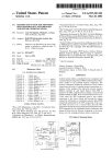
Figure 1-1: Basic concept of PCR amplification ................................................................ 1
Figure 1-2: Chemical structure of nucleoside triphosphates............................................... 3
Figure 1-3: Typical thermal recipe for PCR ...................................................................... 8
Figure 1-4: PCR schematic illustrating selective amplification of the target region
between the primer pairs................................................................................................... 11
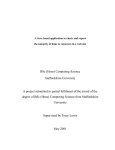
Figure 1-5: MJ Thermal Cycler from Bio-RAD .............................................................. 13
Figure 1-6: Chemical Structure of SYBR Green I............................................................ 16
Figure 1-7: Fluorescence spectrum of SYBR Green I ..................................................... 17
Figure 1-8: Schematic of TaqMan probes ........................................................................ 18
Figure 1-9: Amplification plots for a calibration curve. Replaces 16–20 are 10-fold serial
dilutions............................................................................................................................. 20
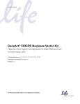
Figure 1-10: Calibration curve for an M13 virus DNA sample........................................ 21
Figure 1-11: Strategene MX3005P benchtop RTPCR system.......................................... 23
Figure 1-12: Serial dilutions to determine sensitivity of assay......................................... 24
Figure 1-13: Assay specificity .......................................................................................... 25
Figure 2-1: Basic schematic of photolithography ........................................................... 28
Figure 2-2: Photolithography using a stepper.................................................................. 31
Figure 2-3: Example of bulk micromachining.................................................................. 32
Figure 2-4: PDMS micromolding ..................................................................................... 36
Figure 2-5: Surface micromachining ................................................................................ 38
Figure 2-6: Chemical Structure of Parylene ..................................................................... 40
Figure 2-7: Schematic of parylene CVD deposition......................................................... 42
xiii
Figure 2-8: Chemical structure of di-p-xylylene, the dimer precursor to parylene N .... 42
Figure 2-9: Surface micromachined parylene channel ..................................................... 46
Figure 2-10: Embedded channel technology .................................................................... 49
Figure 2-11: Microfluidic components fabricated using parylene technology................. 51
Figure 2-12: Thermal isolation by parylene “stitches” ..................................................... 52
Figure 2-13: Integrated HPLC system .............................................................................. 53
Figure 2-14: QPCR on low volumes in parylene coated tubes........................................ 53
Figure 2-15: Amplification of 0.5 μl QPCR solution ...................................................... 54
Figure 2-16: QPCR with various S.A./volume ratios of Parylene-C............................... 55
Figure 2-17: High SA/vol ratios of Parylene on a 0.5uL RTPCR sample....................... 57
Figure 2-18: Concept of an effective distance “h” in which PCR is inhibited ................ 58
Figure 2-19: QPCR with various S.A./volume ratios of Parylene-HT ............................ 59
Figure 2-20: QPCR with glass added into reaction tubes ................................................. 60
Figure 3-1: Overall process flow ..................................................................................... 62
Figure 3-2: Silicon chip ................................................................................................... 63
Figure 3-3: Patterned oxidation layer .............................................................................. 64
Figure 3-4: Metal deposition and patterning. Oxide layer (purple) underneath the metal
(orange) acts as in electrical insulator............................................................................... 65
Figure 3-5: DRIE etching of the bulk silicon. The sides of the channels and the slots
where parylene will fill and make stitches are etched. ..................................................... 66
Figure 3-6: First parylene deposition............................................................................... 67
xiv
Figure 3-7: Inlet-outlet formation. Notice the back side etching (shaded in brown)
overlaps the channel etching region, ensuring a continuous path when the channel is
etched. ............................................................................................................................... 68
Figure 3-8: Etching of first parylene layer (light blue) and XeF2 etching of underlying
silicon................................................................................................................................ 69
Figure 3-9: Inlet outlet hole ............................................................................................. 69
Figure 3-10: Second parylene patterning. Underlying oxide is once again the top layer.71
Figure 3-11: Air gap formation......................................................................................... 72
Figure 3-12: Zoom showing the parylene “stitches” used to connect the island to the main
body................................................................................................................................... 72
Figure 3-13: Wire bonding on the completed chip. The wire bonds provide electrical
continuity across the parylene-stitched air gap................................................................. 73
Figure 3-14: Bubble trapped in reaction chamber from early chip designs..................... 74
Figure 3-15: Channel layout ............................................................................................. 75
Figure 3-16: Channel cross section................................................................................... 76
Figure 3-17: EE analogue for thermal characterization................................................... 80
Figure 3-18: Thermally isolated island ............................................................................. 82
Figure 3-19: Parylene stiches............................................................................................ 83
Figure 3-20: Extended RC Model..................................................................................... 83
Figure 3-21 Temperature sensor calibration ..................................................................... 85
Figure 3-22: Temperature control hardware arrangement ............................................... 87
Figure 3-23: Steady state temperature ............................................................................. 88
Figure 3-24: Heating with step function applied power ................................................... 89
xv
Figure 3-25: Temperature cooling dynamic with zero applied power.............................. 90
Figure 3-26: Chip housing assembly ................................................................................ 91
Figure 3-27: Chip housing components............................................................................ 92
Figure 3-28: Chip housing with external valves .............................................................. 93
Figure 3-29: Structure of the M13 virus ........................................................................... 94
Figure 3-30: Genome of the M13 virus ............................................................................ 95
Figure 3-31: Temperature recipes..................................................................................... 96
Figure 3-32: Filter block for SYBR Green I detection ..................................................... 97
Figure 3-33: SYBR Green fluorescence in microchannel .............................................. 100
Figure 3-34: Detection of M13 virus. Data normalization described above................... 101
Figure 3-35: Air gap chip versus conventional QPCR machine.................................... 102
Figure 4-1: Overall device fabrication steps.................................................................. 104
Figure 4-2: Bare silicon chip.......................................................................................... 105
Figure 4-3: Oxide layers. Notice the back side shows silicon etched by the DRIE. Back
side also shows the “legs” of the front side oxide pattern for clarity. Actual silicon is not
transparent....................................................................................................................... 105
Figure 4-4: First parylene layer with representative holes. The holes are actually present
throughout the outlined channel region. ......................................................................... 106
Figure 4-5: Channels etched into silicon. Bottom right is i/o hole. .............................. 107
Figure 4-6: Second parylene layer deposited................................................................. 108
Figure 4-7: Platinum pattern .......................................................................................... 109
Figure 4-8: Back side finishing. View from back side. Left: After DRIE. Right: After
XeF2 ................................................................................................................................ 110
xvi
Figure 4-9: Finished chip front and back....................................................................... 111
Figure 4-10: Platinum traces directly on parylene. Left: contact pads. Right: heaters113
Figure 4-11: Metal layout .............................................................................................. 113
Figure 4-12: Temperature sensor calibration.................................................................. 115
Figure 4-13: Simple circuit analogy ............................................................................... 116
Figure 4-14: Thermal resistance to heat transfer into environment ............................... 118
Figure 4-15: Cooling experiments used to determine thermal time constant and
capacitance...................................................................................................................... 120
Figure 4-16: Heating experiments .................................................................................. 120
Figure 4-17: Chip housing assembly. O-rings and pins not shown .............................. 121
Figure 4-18: Chip housing components......................................................................... 121
Figure 4-19: Detection of M13 virus on chip ................................................................. 123
Figure 4-20 Comparison of chip versus conventional machine. Sample volumes and
surface-area-to-volume ratios of parylene were comparable.......................................... 123
xvii
List of Tables
Table 1-1: Technical specifications for the Bio-Rad MJ Mini PCR Machine................. 13
Table 2-1: Methods for etching silicon............................................................................ 32
Table 2-2: Physical values of parylene (Unless otherwise stated, values are from ref 17)
........................................................................................................................................... 41
Table 3-1: Thermal conductivity of selected materials.................................................... 77
Table 3-2: Values for calculation of Rayleigh number for air......................................... 79
Table 3-3: Nusselt numbers. All correlations from CRC Handbook47 ........................... 80
Table 3-4: Power specifications for the air gap version .................................................. 86
Table 3-5: Parameters used for thermal model ................................................................ 90
Table 4-1: Parameters for heater.................................................................................... 116
1
1 PCR and Real Time PCR
1.1 Introduction to the Polymerase Chain Reaction
The polymerase chain reaction (PCR) is an in vitro molecular biology technique
used to amplify deoxyribosenucleic acids (DNA). Developed primarily by Kary Mullis
(Nobel Prize, Chemistry 1993) while at Cetus Corporation in the 1980s, PCR is now a
standard technique used in nearly all biology labs in the world. Using the reaction,
scientists can amplify a target region of DNA located within the template DNA (Figure
1-1).
The product is called the amplicon.
This technique greatly simplifies DNA
amplification which before the development of PCR required DNA to be reproduced in
vivo in bacteria using cloning techniques. The amplification of a specific target region
makes PCR an exceptional tool for a wide variety of applications including paternity
tests, genotyping, and pathogen detection.
Template DNA
Target region
Figure 1-1: Basic concept of PCR amplification
2
To explain PCR in detail, a list of components will be provided, followed by the
procedure, equipment, and applications.
1.1.1 Components
To prepare the reaction, the components of PCR are mixed together in a thin walled (for
improved heat transfer) test tube. Oftentimes this tube will be certified as DNAse free to
prevent degradation of the template and products by the DNAase enzymes.
The
components are commonly placed inside a bucket of crushed ice to minimize reactions
while mixing. Below is a list of components. The order of the list does not reflect the
order in which reactants are added.

The DNA template is the original source DNA that contains the target region. This
can be as simple as a synthesized strand of single stranded DNA or the entire genome
of an organism. In reverse transcriptase PCR, the template is a strand of RNA which,
before the reaction starts, is reverse transcribed by the reverse transcriptase enzyme
into the corresponding complimentary DNA (cDNA). Depending on the assay, some
sample preparation may be required to obtain a suitable template material. For
example, tissues have to be treated to access cells, which then are lysed into a
suspension that undergoes DNA extraction using a glass solid phase chromatography.
Care must also be taken to ensure contaminants from the sample preparation steps do
not inhibit the PCR reaction.

Deoxynucleoside triphosphates (dNTPs) are the monomeric building blocks of DNA.
The standard set of dNTPs used consists of: deoxyadenosine triphoshate (dATP),
deoxyguanosine triphosphate (dGTP), deoxythymidine triphosphate (dTTP), and
3
deoxycytidine triphosphate (dCTP). They are composed of a ribose sugar, three
phosphate groups, and a base (Figure 1-2). The base component determines the type
of nucleotide it is. RNA has an OH group at the 2’ of the ribose sugar while DNA
has only a hydrogen atom there. For normal PCR operation, equal ratios of the four
standard dNTPs are added to the reaction mix. Deviation from the standard recipe
can be useful for special applications. For example, to study random mutations to the
target region, one of the dNTPs can be added in excess to increase the chance of
erroneously incorporating that nucleotide into the amplicons. For other applications,
slight variants of the standard nucleotides can be used. Deoxyuridine triphosphate
(dUTP) can be substituted along with biotin or fluorescently labeled variants of
dUTP.
These modified nucleotides provide useful functions such as binding to
streptavidin and detection by fluorescence, two properties that are heavily exploited
in biochemistry and biotechnology.
Figure 1-2: Chemical structure of nucleoside triphosphates1
4

The two DNA primers are short (20–100 bases) single stranded pieces of DNA that
flank the target region within the DNA template. See Figure 1-3 and Figure 1-4, for
an illustration as to why the primer pair defines the target region. When they bind to
the template, they define the starting point of amplification. The starting point of one
strand is the ending point of its complimentary strand. Thus, after a few cycles all the
products start and end at the DNA primers. These primers can be synthesized inhouse or easily obtained from a vendor such as Integrated DNA Technologies2.
Design of these sequences can be complicated, but software such as MIT’s Prime3
exists to facilitate the primer design process3. Some guidelines are given below:
o The sequences should be designed such that the target DNA is contained
between the primers and is about 100–1000 base pairs (bp) in length.
o Sequence length should be about 15–30 bases long. Sequences that are
too short lack specificity.
To illustrate this point, consider that the
complementary sequence of a primer of length 1 can be found in ¼ of the
sequences of length 1. For length 2, about 1/16 of the length 2 sequences
are complimentary. For length 16, only one in set of 4.3 X 109 (416, about
the length of the human genome) random 16-mers will match. Thus,
sequences should be larger than about 16 bases. The upper limit is driven
by specificity as well. An extremely long primer will base pair despite a
single-base mismatch because the other correct pairings provide enough
thermodynamic driving force to sustain one mismatch. The most common
primer lengths used are about 20 bases long. Within these 20 bases, the 3’
end of the primer is most important since Taq DNA Polymerase will
5
extend this end when assembling the new strand even if the 5’ end is
slightly mismatched and not binding efficiently. In fact, the 5’ end can be
modified to carry additional sequences such as restriction sites that are not
complementary to the template.
o The melting temperature (Tm) of primers should be about 52–58oC. This
is the temperature above which the DNA separates from its compliment to
become two single strands of DNA. Tm that is too low will require a low
annealing temperature that allows nonspecific primer binding while
temperatures should not be higher than the elongation temperature as
DNA synthesis will prematurely start. The annealing temperature is often
set at 5oC lower than the lower Tm of the two primers to start then further
optimized using trial and error. A simplified correlation for estimating the
melting temperature for primers is:
Tm ( o C )  4(G  C )  2( A  T ) Equation 1-1
Where G,C,A,T represent the number of instances of the respective
bases.
o Primers should not contain sequences that result in secondary structure.
This structure occurs when two regions of the primer compliment each
other, causing the DNA strand to curve and bind to itself much like tape
sticking to itself.
This shields the primer DNA from accessing the
template DNA. Furthermore, primers should not be complementary to
each other to avoid primer-dimer formation. Partial dimer formation will
result in amplification of the primers themselves.
6
o In some cases, mispriming is specifically designed into the primers. Point
mutations (a difference of one nucleotide between the mutant and original
DNA strand) can be introduced into DNA sequences by first introducing
them into primers.
Larger sets of nucleotides such as a restriction
endonuclease recognition site can be added to the 5’ ends of primers to
allow the amplicons to be inserted into a cloning vector and expressed in
bacterial cells. These techniques are part of the field of molecular biology
enabled by PCR: molecular cloning.

DNA Polymerase is an enzyme that continues synthesis of a complementary strand of
DNA. In the early implementations of PCR, E.Coli DNA polymerase (in particular,
the Klenow fragment) was destroyed at the melting DNA temperatures (~95oC) and
thus replaced after every cycle. Furthermore, the ideal temperature for synthesis
using this polymerase was 37°C; however, this allowed primers to bind to
noncomplementary regions thus reducing specificity. Biologists eventually moved to
Taq Polymerase I because it is thermally stable at 95oC. This move is considered by
many as the most important development towards the wide usage of PCR4. Taq
polymerase was originally isolated from Thermus aquaticus bacteria that live in hot
springs and thus have polymerase that can withstand high temperatures. The enzyme
has optimal activity around 70–80oC, and a half life of about 10 minutes at 97oC.5
Not only did this lead to survivability at the denaturization step, it allowed higher
annealing temperatures which lead to increased primer binding specificity and
reduction in secondary structures in the template and target strands. At the optimal
temperature, Taq polymerase has an estimated extension speed of about 60
7
nucleotides per second. For the ~120 bp target region in this study, this would mean
a minimum of 2 seconds is required for the DNA synthesis step; however, the
processivity (average number of nucleotides incorporated until the polymerase
dissociates) of the enzyme is only about 60 nucleotides thus a full 15 seconds is used.
The enzyme also features a 5’  3’ exonuclease activity, meaning it can destroy a
pre-existing strand of DNA that is in front of it when synthesizing the new strand.
This feature is useful for FRET-based real time PCR, discussed in Section 1.2.2.2.
Taq polymerase used in modern reactions are recombinant (i.e., have an altered
protein sequence) and packaged with molecules that disable activity at room
temperature but restore full activity upon heating to 95oC (“hot start” polymerase).
Invitrogen’s Taq polymerase contains anti-Taq polymerase antibodies that serve this
function6. One major disadvantage of Taq polymerase is the lack of a “proofreading”
ability, resulting from random errors in replication (about 1 per 104 nucleotides4).
Since the errors are random, they are not significant for most applications of PCR
since a given site has an overwhelming number of correct nucleotides compared to
the erroneous ones. For applications where even slight errors are not tolerable, DNA
polymerase from other organisms such as Pyrococcus furiosus and Thermococcus
Litoralis can be used.

The buffer solution maintains the optimal pH and salt concentration values for
efficient amplification. This solution is often purchased from a vendor in a pre-mixed
form. It is typically a Tris-HCl buffer system around pH 8.4 with KCl and some
MgCl2 already added. Of particular importance is the concentration of Mg2+ ions that
are often supplied separately since each reaction condition requires a different
8
concentration. The ions function as a cofactor for Taq polymerase and also enhance
the ability of primers to bind to the target/template DNA. Excess Mg2+, however,
causes Taq DNA polymerase to become more error prone4. The buffer solution may
also be tested for the absence of DNase and RNase, enzymes that degrade DNA and
RNA, respectively.
1.1.2 Procedure
The PCR reaction solution is assembled to a total of 20–100 μL in a plastic thin walled
reaction tube and placed in a thermal cycler for 30–40 cycles.
(minutes)
Figure 1-3: Typical thermal recipe for PCR
A typical thermal recipe is:
9
1. 940C for 2 minutes. This initialization step activates specially modified Taq
polymerases which are designed for minimal activity at room temperature. Also,
during this step the template DNA and primers fully dissociated. This step occurs
only once in the reaction.
2. 940C for 15–30 seconds. This denaturation step dissociates the DNA targets (also
called amplicons) produced during previous cycles by disrupting the hydrogen
bonds between complementary bases. This exposes the bases and allows the
primers bind to them in the next step.
3. 550C for 15–30 seconds. During this annealing step, the primers bind to their
complementary sequences in the target DNA.
4. 720C for 15–30 seconds. This is the extension step when the DNA polymerase
extends the DNA strand starting from the primers, assembling from the 5’ to 3’
end of the new DNA strand by adding the complementary dNTP to the elongating
strand.
5. Repeat steps 2–4 for about 30–40 cycles. After each cycle, the number of DNA
molecules is theoretically doubled if 100% efficient.
6. Final Elongation. This step is often performed at 720C for 5 minutes to ensure
any remaining single-stranded DNA is fully extended.
The exact temperatures and times used vary from reaction to reaction. For a given
reaction, a series of conditions must be tested to find an optimal set. Here are some
guidelines for choosing a thermal recipe:
10
o Denaturation step: Increasing temperature causes faster breakdown of Taq
polymerase while lowering the temperature below the melting point of the
target DNA would halt replication.
o Annealing step: This temperature varies the most as it has the most effect
on PCR. Too high temperature will result in reduced products since a
smaller fraction of primers can overcome the thermal energy required to
remain bonded. Too low temperature is also detrimental as it allows
primers to bind nonspecifically, resulting in multiple products, seen as
multiple bands on gel electrophoresis.
Low temperatures promote
secondary structures on DNA.
o Extension step: Excessively high or low temperatures will result in non-
optimal performance by Taq polymerase.
11
Figure 1-4: PCR schematic illustrating selective amplification of the target region between the
primer pairs7.
12
1.1.3 Molecular Level Theory
In Figure 1-4, step 1 refers to the denaturalization of the template forming two single
stranded pieces of DNA. Step 2 shows the annealing step where the primers bind. Step 3
is the elongation step. Notice that although elongation starts at the primer, it ends when
the polymerase (labeled with a P) simply runs out of template to replicate. For the
template molecules, this end can be incredibly far from the primer binding region,
creating extra-long products. These products, when used in the next cycle, however,
produce products whose length is the region between the primers (step 4). It can be seen
that after the first few cycles, the majority of products (also called amplicons) will
contain only the target region while the original templates and extra-long products
become a minority. A more quantitative description will be provided in the next chapter.
1.1.4 Equipment
The main piece of equipment required to perform PCR is a thermal cycler.
Such a
machine attempts to cycle between the relevant temperatures as quickly as possible. In
early implementation of PCR, the scientist would manually transfer the PCR mixture
from one water bath to the next. Furthermore, before the Taq DNA polymerase came
into usage, PCR required addition of fresh E. coli DNA polymerase after each denaturing
step. Modern machines have one computer-controlled heating block that cycles through
temperatures at programmed times. The machines also have a heated cover that keeps
the caps of the reaction tubes at 105oC. This prevents condensation of the water vapor on
the cap, which in turn keeps the concentrations and pH of the reaction solution constant.
13
A typical machine is the Bio-Rad MJ Mini Gradient Thermal Cycler (Figure 1-5Error!
Reference source not found.). Some specifications are provided in Table 1-1 below8:
Table 1-1: Technical specifications for the Bio-Rad MJ Mini PCR Machine
2.50C/s
400W max
19 x 32 x 20 cm
4.1 kg
Ramping speed
Input power
Dimensions (WxDxH)
Weight
Figure 1-5: MJ Thermal Cycler from Bio-RAD
Currently PCR machines are relatively large, heavy, slow, and require hundreds of watts
power. The use of a bulky thermal block causes slow temperature ramp rates. These
issues can be addressed using MEMS technology.
1.1.5 Gel Electrophoresis
Following PCR, gel electrophoresis is used to determine if the anticipated DNA target
was amplified. Using this technique, a DNA ladder (mixture of fragments of DNA of
known size) is run alongside the PCR sample to obtain an estimate of the size of the
product (sometimes referred to as the amplicon). If only one product is formed that is of
the anticipated length, one can be reasonably assured that the amplicon is in fact that
14
identical to the target DNA. If further reassurance is required, one can sequence parts of
the amplicon or bind it to a probe strand of known sequence.
1.1.6 Applications
Since PCR is a DNA-based analysis it is versatile due to the fact that all organisms
have DNA or RNA which can be converted to DNA. The usage of DNA primers takes
advantage of the naturally evolved base pairing phenomenon that provides excellent
specificity. The assay is also practical because tests can be performed in about one hour
using a few pieces of equipment that are standard in modern biology laboratories and
using cheap, easily obtainable reagents.
PCR can supply large amounts of specific DNA for further analysis and can be
used “downstream” from other assays. This is particularly useful when only small
amounts of the original template DNA is present such as in forensic analysis. It can be
used to isolate a specific region of DNA for purposes such as bacterial transformation and
is a central part of the Sanger sequencing method for determining the sequence of DNA
fragments. Perhaps the most well known application of PCR is DNA fingerprinting used
in criminal trials. DNA fingerprinting can also be used in paternity testing and even
determine evolutionary relationships between organisms.
By designing primers that
amplify a DNA sequence that is unique to virus, one can identify its presence in a sample.
PCR can also be used to diagnose diseases such as cancer.
15
1.2 Real Time PCR
The real time polymerase chain reaction (RTPCR) or quantitative polymerase chain
reaction (qPCR) is a procedure based on PCR where a piece of target DNA is both
amplified and quantified (using fluorescence) simultaneously.
1.2.1 Theory
From the background of PCR, it is seen that the number of DNA target molecules
doubles after every cycle. Mathematically, this can be written as:
T  T0 * 2 c Equation 1-2
where
T = current number of target molecules
T0= initial number of target molecules
c = number of cycles
Furthermore, if one allows for a nonidealistic efficiency, the value “2” can be substituted
with (1+E) where E ( 0 < E < 1 ) is the average efficiency after c cycles. Thus, Equation
1-2 becomes:
T  T0 (1  E ) c Equation 1-3
Since we choose a constant value for E here Equation 1-3 is only valid for the early
cycles, before the efficiency becomes unpredictable due to a variety of factors such as
degradation of Taq polymerase after repeated thermal cycling. These early cycles are
referred to as the “exponential phase” and their termination can be identified by the
16
deviation in exponential shape of a T versus c curve or deviation of linearity in a log (T)
versus c curve.
1.2.2 Fluorescent Indicators
1.2.2.1 SYBR Green
SYBR Green I (SG) is a nucleic acid stain with many uses including double stranded
DNA (dsDNA) quantification in real time PCR and gel electrophoresis. For the latter, it
is generally considered a safer alternative to ethidium bromide, with 25X better
sensitivity. Upon binding to double stranded DNA, its fluorescence intensity becomes
1,000 times that of its unbound state, with a quantum yield of ~0.8.9 This large gain in
fluorescence contributes to a good signal-to-noise ratio as non-bound SG in the solution
and walls of the container contribute minimal noise. Its chemical structure is shown in
Figure 1-6. At low concentrations, the dye binds to DNA by intercalation; however, at the
higher working concentrations for qPCR, surface binding dominates (evidence suggests
the surface binding occurs at the minor groove of dsDNA)10. The stock stain solution
comes dissolved in DMSO (dimethylsulfoxide) and stored frozen (-20oC) until use. After
a 10,000X dilution for RTPCR analysis, the working concentration is about 2 μM.
Figure 1-6: Chemical Structure of SYBR Green I
17
Its double stranded DNA-bound fluorescence spectrum is available in Figure 1-7.
Figure 1-7: Fluorescence spectrum of SYBR Green I11
Since SYBR Green I binds to all double stranded DNA (at the working concentrations), it
can be used irrespective of target DNA sequence, making it versatile. As the number of
double stranded DNA molecules increases, so does the fluorescence. This feature is also
its biggest limitation as non-specific (non-target-DNA) sequences that are unintentionally
amplified also produce a fluorescence signal. This limitation is partially addressed by the
generation of melting curves and gel electrophoresis to check for purity and length of the
product. Removal of SYBR Green from DNA can be achieved by ethanol precipitation.
Add ethanol to cause the DNA to precipitate, then centrifuge the pellet, wash it again in
ethanol, allow to dry, then resuspend in buffer solution.
18
1.2.2.2 TaqMan
An alternative to SYBR Green I are the family of TaqMan probes. These have
the advantage of fluorescing only during the synthesis of the target DNA, thus adding
another level of specificity. A schematic of the TaqMan probe system is shown in Figure
1-8.
Figure 1-8: Schematic of TaqMan probes
In its free state, the green and red fluorophores are connected via the DNA bases
between them. These bases are designed to be complementary to a sequence within the
target DNA. The proximity allows Förster resonance energy transfer (FRET) to occur:
the energy from the optically excited green fluorophore (donor molecule) transfers to the
red fluorophore (acceptor molecule) which accepts and dissipates the energy as heat or
19
light in a longer wavelength. During the annealing step of RTPCR, the TaqMan probe
binds to its complementary sequence on the target DNA (step labeled as “anneal” above).
During the extension step, as Taq DNA polymerase extends the target DNA, it destroys
the seemingly disruptive Taqman probe as it synthesizes the new strand. This allows the
green fluorophore to become spatially separated from the red quenching molecule, thus
emitting its green photons instead of participating in FRET. This increase in fluorescence
is then measured by the RTPCR machine.
This mechanism is key to the added specificity provided by the Taqman system.
If the target DNA does not exist, the probes will not bind and thus not be destroyed by
DNA polymerase. Also if the target region is present but the primer pairs fail to function
correctly no fluorophore is emitted. The specificity of the Taqman system limits its
scope in usage. Custom probes must be synthesized for each target, increasing costs for
research.
1.2.3 Calibration Curves
The key that allows real time PCR to be quantitative is the relationship between the
starting number of template DNA molecules and the number of cycles required to
amplify it to a set amount. If there are more starting molecules, fewer cycles are
required. Below is an example of how a calibration curve is obtained followed by an
analysis of the process.

Obtain a sample of known template DNA concentration

Prepare 10 fold serial dilutions to generate multiple data points for the curve

Perform RTPCR on these samples
20
The data from these steps results in a graph such as the one below:
Figure 1-9: Amplification plots for a calibration curve. Replaces 16–20 are 10-fold serial dilutions.

From the above data, choose a “threshold” fluorescence value (blue solid line)
that crosses the sample curve where they are all linear (in a log-fluorescence
versus linear cycle number plot)

Note the number of cycles required by each known concentration to reach the
threshold fluorescence, call it ct and plot it against the concentration
These steps yield a curve such as shown in Figure 1-10:
21
Calibration Curve
25
Threshold Cycle Number
20
15
10
5
0
0.001
0.01
0.1
1
10
100
Concentration (ug/m l)
Figure 1-10: Calibration curve for an M13 virus DNA sample
From this plot the concentration of an unknown sample (assuming identical experimental
conditions) can be estimated by observing its threshold cycle number. Using linear
regression, a relationship for this curve yields:
Ct  3.423Log (T0 )  11.33
E  95.9%
Equation 1-4
where
Ct is the number of cycle required to reach the threshold fluorescence
T0 is the initial concentration of template DNA molecules
E is the efficiency of the reaction
22
A mathematical derivation of
Equation 1-4 is now given.
By rearranging
Equation 1-3, the relationship between starting DNA copy number T0 and cycle number
c can be derived using simple algebra as:
1
log(T )
Equation 1-5
log(T0 ) 
log(1  E )
log(1  E )
c
To find a one-to-one correlation, the parameters T and E must be kept constant. For a
constant value of target molecules T, we choose a set value for the threshold fluorescence
(this assumes a linear relationship between fluorescence reading and number of target
molecules which is generally a good assumption) and call it Tt. To obtain a constant
efficiency E we narrow the range of threshold fluorescence values to only when the
reaction is in the “exponential phase” or the linear phase in a log plot. When T = Tt, the
observed c is the threshold cycle number, ct. Thus,
ct 
log(Tt )
1
log(T0 ) 
Equation 1-6
log(1  E )
log(1  E )
If m is the slope of a ct versus log(T0) plot, the efficiency E can be calculated:
m
1
 E  10 1 / m  1 Equation 1-7
log(1  E )
1.2.4 Equipment
There are many manufacturers of real time PCR machines including BioRAD,
Applied Biosystems, Roche, Cepheid, and Strategene. The “entry level” models from
these manufacturers are very similar, most featuring an LED or halogen light source,
23
peltier-based heating and cooling, CCD or photodiode photodetectors with rotating filter
wheels, and a thermal block that fits standard 48 or 96 well plates. These machines
typically cost around $30,000, weight 20 kg, use max 10 Amps at 120 VAC, and have a
length scale of about 40 cm. Temperature ramping times are typically 100C/second and
results are obtained in about 1.5 hours.
Some companies seek to differentiate their machines with slight modifications.
The Roche Light Cycler 2.0 has a rotating carousel of capillary tubes instead of a 96 well
plate thermal block. In this design, temperature distribution is more uniform as a fan
blows heated or cooled air past the rotating carousel. The Applied Biosystems StepOne
model is a standalone unit that does not require a computer and has its own touch-screen
interface. The Strategene MX 3000P and MX 3005P models (shown below) feature a
scanning photodetector unit comprised of a fiber optic cable leading to a photomultiplier
tube with a 5 color filter wheel.
This design eliminates non-uniformity in the
fluorescence detection, a problem faced by the CCD image capture approach.
Figure 1-11: Strategene MX3005P benchtop RTPCR system
1.2.5 Applications
Two applications of real time PCR are described below: pathogen detection and mRNA
expression profiling.
24
1.2.5.1 Pathogen Detection
Pathogen detection is a popular application of real time PCR. The versatility of
this technique is demonstrated by Zeng et al12 as they detect the airborne mold
Cladosporium, an allergen. They determined the presence of 104 spores/m3 in two
locations: a countryside house that houses firewood and a paper factory. A higher level
at 107 spores/m3 was detected in a cow barn.
These levels exceed the medically
recommended maximum exposure of 3000 spores/m3. Prolonged exposure can weaken
the immune system and cause severe asthma. In past studies, detection of Cladosporium
was based on slower methods including cell culture, in which spores were grown in an
incubation chamber before microscopic identification by eyes, a time-consuming and
labor-intensive approach.
To test the sensitivity of their array, they performed a serial dilution test (Figure
1-12). The most dilute sample detected (labeled #6) corresponded to only 2 spores. This
sensitivity of down to 1 genome copy is not uncommon in RTPCR assays.
Figure 1-12: Serial dilutions to determine sensitivity of assay13
25
To test for specificity, the authors performed the same assay on different types of
fungi (Figure 1-13). The various species of Cladosporium gave a typical signal while
other types of fungi showed virtually no signal.
Figure 1-13: Assay specificity
1.2.5.2 mRNA Expression Profiling
As described in the earlier section, real time PCR allows quantification of initial
template DNA amount when compared against a calibration curve. An extension of this
technique is to quantify the amount of specific messenger ribonucleic acid (mRNA)
expressed in a cell or tissue by first reverse transcribing the mRNA into complementary
DNA (cDNA). This technique is referred to as reverse transcription quantitative PCR
(RTqPCR). Some authors also call this technique RTPCR, so care must be taken to
distinguish between “real time” PCR and “reverse transcription” PCR.
Upon stimulation, cells will undergo a “signal transduction” process resulting in the
transcription of mRNA which travels from the nucleus (where the DNA is) into the
cytoplasm to be translated into proteins and enzymes. Quantification of amounts of a
particular mRNA gives insight into a cell’s natural function and reaction to stimuli such
as drugs or signaling molecules from other cells and is of great importance in the field of
26
biology. Although there are various methods, in recent years RT-QPCR has emerged as
the method of choice for this analysis14.
1.3 Chapter Summary
Requiring simple, affordable machinery and components, real time PCR is easy to
implement for extension of PCR that provides a new dimension to PCR analysis. By
monitoring the amount of DNA present via fluorescence, quantification of the initial
amount of DNA or RNA in the sample can be achieved.
27
2 Parylene Microfluidics
This chapter serves as a short introduction to microfluidics including some
background, reasons for using microfluidics, and basic technologies.
Parylene as a
microfluidics material is discussed in the middle of the chapter and microfluidics as
applied to real time PCR is discussed towards the end.
2.1
MEMS Background
The microelectronic industry has greatly matured since the discovery of the
transistor effect in semiconductors in the 1940s. Whereas early computers filled entire
rooms and were only accessible to a few users through terminals, today portable “smart”
cell phones have far superior computational power packed into a hand-held device.
These devices are small, light, and affordable.
Such a dramatic change in capabilities and portability in electrical and
computational devices has inspired an analogous effort in the mechanical and biological
realms using similar technology. Since MEMS was born from microelectronics, both
fields share similarities in materials and patterning technology. Recently, however, with
increasing interest in biological assays in MEMS, new materials and methods are being
introduced that are more biocompatible.
2.2
General Microfluidics Technology
At the core of microfluidics technology is photolithography: using an energy beam
to pattern thin photosensitive films (called photoresists).
The energy beam can be
composed of photons (light, UV), electrons, X-ray photons, or even ions. In this work
28
only UV photons are used. The thin films used depend on the energy source but their
general principle is shown in Figure 2-1.
Figure 2-1: Basic schematic of photolithography 15

Film deposition:
A thin film to be patterned is deposited onto a substrate.
Because MEMS originated from microelectronics, silicon is still commonly used
as a substrate. The thin film can be silicon oxide, silicon nitride, metal, poly
silicon, or a polymer. Often it is the silicon itself that is to be patterned, in which
case no thin film is deposited.

Photoresist application:
To pattern a thin film deposited on a substrate, a
photosensitive photoresist layer is deposited. This is often performed by placing
the substrate on a spinner, pouring the photoresist suspension onto a wafer then
spinning between 1000–8000 rpm, depending on the desired thickness and
viscosity of the suspension. The casting solvent is then removed by evaporation
in an oven or hot plate.
29

Exposure: A light source such as a mercury lamp is used to supply energy while a
mask is used to supply the pattern. This mask itself is usually a glass plate with
patterned chromium as the reflecting layer. The photoresist reacts to the light in a
way that changes its solubility in a developer solution. One example of this
process is the DQN family of photoresists. They are comprised of a photoactive
diazoquinone ester (DQ) and a phenolic novolak resin (N). Upon exposure, the
DQ undergoes a photochemical reaction that makes the DQN soluble in a basic
developer solution while the unexposed regions remain insoluble18. Some types
of resists also require a post-exposure bake to speed up reactions that initiated
during exposure.

Development: During this step, the wafer is exposed to a solution that selectively
dissolves only the portions of the photoresist that has been exposed to UV. For
“negative” photoresists, the portions that were not exposed are dissolved. The
wafer is then rinsed and dried, resulting in a patterned photoresist layer. At this
time, the resist is often “hard baked” or “post baked” by placing into an oven or
hotplate to further drive away remaining development solution, casting solvent, or
moisture, resulting in a hardened film with increased resistance to etching
environments. A mild oxygen treatment referred to as “de-scumming” may also
be executed here to etch away any photoresist residue that may not have been
developed away.

Etching: With the photoresist in place, the wafer can be placed into an etching
environment such as a plasma or acidic metal etching solution. The photoresist
30
protects the layers that are underneath it from the etchant such that the thin film’s
pattern matches the resist pattern.

Resist removal: After etching, the resist has served its purpose and can now be
removed. A photoresist stripper solution can be purchased from the resist vendor.
Some resists easily dissolve in common organic solvents such as acetone.
A key feature of the photolithography process is that features can be mass produced
on wafers. As seen in Figure 2-2, the pattern from one mask can be projected onto a
wafer repeatedly to make tens to hundreds of devices simultaneously. This projector can
also reduce the size of mask features, for example, by a factor of 10. The optical limit for
feature sizes is given by Rayleigh’s criteria:
Wmin 
k
Equation 2-1
NA
Where k is a constant related to the contrast of the photoresist (typically 0.75), NA is the
numerical aperture of the projection system (about 0.6), and λ is the wavelength of light
used (365 nm). In this example, the minimum feature size under the optical limit would
be about 0.5 μm16.
As a result of these basic fabrication features, MEMS devices are smaller, lighter,
and possibly cheaper. In some cases performance is improved and potential integration
of many functions onto one chip exists.
31
Figure 2-2: Photolithography using a stepper17
2.3
MEMS Technologies for PCR Microdevices
The general outline of photolithography given above is now extended to include
MEMS techniques that are of particular interest in making PCR microdevices.
2.3.1 Bulk Micromachining
Bulk micromachining refers to the fabrication schemes that form a fluidic channel
by etching into the substrate (glass or silicon) then bonding to a cover unit (also glass or
silicon).
32
Figure 2-3: Example of bulk micromachining
Silicon is often used as a substrate because of the wide variety of etching methods
already developed for it and the potential of starting fabrication with a pre-fabricated
CMOS chip.
Both isotropic and anisotropic wet and dry etching technologies are
available (see Table 2-1).
Table 2-1: Methods for etching silicon
Wet Etching
Dry Etching
Isotropic
HNA
XeF2
Anisotropic
KOH
RIE, DRIE
HNA etching is an isotropic mixture of hydrofluoric acid, nitric acid, and acetic
acid to form a solution that oxidizes silicon (caused by the nitric acid), then etches the
oxide (caused by the hydrofluoric acid), subsequently oxidizing the freshly exposed
silicon (caused by the nitric acid). Acetic acid is used as a diluent instead of water
because it prevents dissociation of the nitric acid since oxidation requires undissociated
NHO318. The overall reaction is:
33
Si + HNO3 + 6HF  H2SiF6 + HNO2 + H2O + H2 Reaction 2-1
KOH etching utilizes potassium hydroxide which anisotropically etches the {111}
planes of silicon 30–100x slower than the {100} planes. These solutions are usually kept
at high pH values (>12) and high temperatures (70oC) as they are considerably slower
than the isotropic etching due to the slow chemistry at the surface. One proposed overall
reaction mechanism is:
Si + 2OH- + 2H2O  SiO2(OH)22- + 2H2
Reaction 2-2
In addition to KOH, other oxides used are sodium hydroxide (NaOH), tetremethyl
ammonium hydroxide (TMAH), ammonium hydroxide (NH4OH), and many more.
For dry isotropic etching, XeF2 gas is used. The overall reaction is:
2 XeF2 + Si  2Xe + SiF4
Reaction 2-3
This reaction does not require ion bombardment, heat, or other external energy sources.
Since it is dry and chemical in nature, many masking materials can be used including
aluminum, silicon dioxide, silicon nitride, photoresist, and parylene. These properties
make it useful in post-processing CMOS integrated circuits19. Etch rates are in the 1
μm/min order of magnitude with actual rate highly dependent on silicon load and feature
sizes.
34
Slight anisotropic etching (2:1 aspect ratio) can be achieved using a plasma based
on SF6 (sulfer hexafluoride) and will etch silicon to form the gaseous product SiF4 which
diffuses back into the plasma, creating a new surface to be etched. In the reactive ion
etching (RIE) configuration, a parallel plate chamber is formed, producing a biasing
electric field that drives ions towards the substrate. Since the pressure is in the 300
mTorr range (compared to 2.5 Torr for XeF2), the mean free path is low enough for
slightly directional (in the z direction) etching with a smaller component of lateral
etching caused by interactions between etching molecules.
If true anisotropic etching is required, deep reactive ion etching (DRIE) can be
used. In this modification of the RIE configuration, a SF6 plasma is still used to etch
silicon but the plasma is either alternated with a C4F8 passivation layer for the side walls
(Bosch process) or the substrate is chilled to -110oC (cryogenic process) to minimize
chemical etching rates while preserving the ion bombardment mechanism still present in
the upward facing surfaces.
Another advantage of the ICP configuration is the separation of the plasma power
source and the substrate bias voltage power source. This allows independent control of
plasma density and kinetic energy at which ions bombard the substrate. High densities
mean the plasma is more chemically reactive while lower kinetic energy means
nonspecific mechanical etching (erosion) of mask materials is reduced20. This means
higher specificity which allows for thinner masking materials, which then allows better
in-plane patterning of mask materials since aspect ratios are reduced.
35
To transform the silicon trenches into channels, the fourth wall must be
introduced. This usually occurs by bonding the silicon to either another silicon or glass
wafer. A common technique is anodic bonding, where the silicon is placed in contact
with a special high-sodium glass at 200–5000C and a high DC voltage (~kV) across the
bond. This combination allows the sodium ions in the glass to migrate away from the
interface causing a negative charge on the glass side and a positive charge on the silicon
side. Electrostatic force then holds the two pieces in place to create a water-tight seal.
Early pioneers using this technology to create PCR devices include Peter Wilding
et al. In these early chips, the silicon was etched about 40--80 μm deep and anodically
bonded to Pyrex glass to create reaction chambers between 5–10 μL. An external Peltier
heater and cooler was used for thermal cycling21,22. M.A. Burns et al. published an early
integrated DNA analysis system with PCR chamber, elctrophoresis, and optical detector
by etching glass slides and bonding them to the electrical and optical components on the
silicon23. The glass sealing also allows optical access to the solution while thermal
cycling for usage in real time PCR. The glass and silicon surface of these devices,
however, inhibit the PCR reaction by adsorbing components such as Taq polymerase24 to
an extent that surface treatments such as the addition of BSA must always be used.
Furthermore this scheme uses two rigid materials, complicating the integration of moving
parts such as valves and pumps.
2.3.2 Soft Lithography
Soft lithography generally refers to the use of elastomers such as
polydimethylsiloxane (PDMS) in conjunction with molds to form channels. First, a
master mold is formed by bulk methods such as DRIE of silicon or surface methods such
36
as SU-8 photoresist on top of silicon. A fluid mix of pre-polymer is then poured onto the
master and allowed to cure at 80–100 0C. The PDMS can then be peeled from the master
mold, forming a negative replica. Similar to bulk micromachining, a second surface is
required to complete the channel. Common glass slides work well as they bond well with
PDMS. Surface treatment such as oxygen plasma surface cleaning or application of a
thin adhesion layer of PDMS on the glass slide is often used to enhance bonding.
Figure 2-4: PDMS micromolding
The main advantage of soft lithography is its ease of use. Formation of the master
mold is the only step that requires a clean room environment. Further processing can be
performed in a standard laboratory environment with relatively few pieces of equipment.
Furthermore, PDMS is cheap and easily obtained. Inlet and outlet fluidic connections
become simple: a needle-poked hole is formed which acts as both a gasket and stabilizer
for the capillary tubes. Flexibility allows structures such as pumps and valves to be
integrated with channels. This simplicity has allowed a burst of attention and innovation
to this microfluidics paradigm. Components such as pumps, valves, and mixers have
been fabricated for applications in biochemistry and cell culture25.
Liu et al26
demonstrated a novel rotary device in which a plug of PCR solution was passed through a
circular channel containing 3 heated regions at 94 °C, 55 °C, and 72 °C. The heaters
were fabricated using metal lift-off on the supporting glass slide with tungsten as the
37
heating component with aluminum leads. This design allowed usage of only 12 nL of
solution.
The fluid was pushed by peristaltic style pumps fabricated on a separate
PDMS layer (control layer) on top of a layer of PDMS with the fluidic channels (fluidic
layer).
This control scheme provides the actuation for valves, pumps, and fluidic
metering for large scale integration. The same group later developed the technology to
enable real time PCR on the picoliter scale27. A much simpler design for a PDMS QPCR
device which does not require any photolithography was presented by Q. Xiang, et al.28.
Holes of various sizes (1–7 mm) were punched into an unpatterned sheet of PDMS, while
another PDMS sheet with a larger (5 mm) hole was placed on top. The bottom holes
contained the QCR fluid while the top sheet contained the mineral oil placed on top of the
QPCR solution to prevent evaporation. Using a fluorescent microscope and a CCD
camera, QPCR reactions were performed.
The advantages of using PDMS are its ease of use and flexibility. Disadvantages of using
PDMS arrive from its porosity and surface properties. Evaporation of liquids is common
as solvent vapors penetrate the material. Surface treatments are necessary to prevent biofouling and protein adsorption. The PDMS-glass interface is not capable of supporting
high pressures (over 30 psi). Furthermore, integration into a standard MEMS process or
pre-fabricated CMOS chip is limited to placing a finished PDMS piece on top of the chip.
2.3.3 Surface Micromachining
Surface micromachining involves building structures onto the surface of the
substrate. Channel formation in this case does not require a second bonding step with
38
another wafer. Instead the structural material such as polysilicon is deposited on top of a
sacrificial layer such as silicon oxide. See Figure 2-5.
Figure 2-5: Surface micromachining
In this way all four walls of the channel are already present and the inside is hallowed by
dissolution of the sacrificial layer. If the finished device uses only surface methods, the
substrate may be a cheaper material such as polycarbonate. If polysilicon is used as a
structural layer, biocompatibility will be poor, requiring surface treatments. Flexibility
and ability to integrate movable parts will also be difficult.
An alternative set of
materials are parylene for the structural material and photoresist as the sacrificial layer29.
This scheme will be explored in detail in the next chapter.
2.4
Parylene MEMS Technology
2.4.1 Why Use Parylene?
There are many reasons to use parylene to make microfluidics devices. A brief list of
advantages will be given here followed by more detailed discussion in the sub-sections.
Parylene is a biocompatible material as shown by its USP Class VI classification, which
means the FDA has previously approved its usage in long term human implants. This
39
elite classification translates well into the biochemical arena as it has been shown as a
good material for in vitro experimentation as well. Parylene is chemically inert, able to
withstand various solvents ranging from organic to acidic. This is convenient for testing
purposes as well as during device fabrication where organic solvents are used, for
example, to dissolve photoresist.
Parylene is optically transparent, allowing direct
measurement of fluorescence signals — a requirement for real time PCR. It is flexible
(Young’s Modulus 4Gpa) rather than brittle, allowing formation of a more robust thin
free standing structure/sheet. This also allows for micro-actuation for use in devices such
as on-chip valves and pumps. Since parylene is electrically insulative, metal wires which
serve as heaters and temperature sensors can be placed directly on top of it, making
thermal management more efficient and temperature measurement more accurate.
Parylene also has low permeability to gases which prevents evaporative loss of the pcr
mixture during thermal cycling. Finally, parylene is compatible with various MEMS
processing techniques, which means the usual well established techniques such as metal
deposition and photolithography can be used in conjunction with parylene on the wafers.
Parylene is not a new material.
It has been used in electronics industry as
protective and insulation coatings for circuit boards, wiring assemblies, and as dielectrics
for capacitors because of its resistance to moisture penetration and ability to coat devices
conformally. It has also been used in the biomedical field as microencapsulation for
controlled drug release devices and medical instruments30 because of its inert properties
when interfaced with human tissues. It is thus a natural extension to use parylene in
MEMS and in particular, bio-MEMS applications.
40
2.4.2 Parylene Chemical Structure
The proper chemical name for parylene is poly(para-xylylene). Many variants
exist with varying substitutions on the benzene ring, three of which are down in Figure
2-6:
Figure 2-6: Chemical Structure of Parylene
Variants that have halogens placed in the aliphatic carbons are also available. These
simple chemical changes result in differences in chemical and physical properties as well
as deposition kinetics. In this work, the word parylene will imply Parylene-C unless
otherwise stated.
41
2.4.3 Physical Properties
Below is a list of properties for Parylene-C
Table 2-2: Physical values of parylene31 (Unless otherwise stated, values are from ref
17)
Property
Tensile strength, Mpa
Yield strength, MPa32
Elongation at break, %
Young’s Modulus GPa33
Density, g/cm3
Index of refraction
Melting temperature (°C)
Thermal Conductivity (W/m.k)
Value
69
59
200
2.8
1.289
1.639
290
0.082
Comparison
0.027 times the value for silicon
3.2 times the value for air
Aside from these quantifiable properties, parylene has the distinguished advantage of
being classified as Class VI by the United States Pharmacopeia (USP), a classification
given to materials (and methods which are used to produce them) with superior
biocompatibility suitable for long term implantation in humans. It is also transparent to
light above 300 nm.
2.4.3.1 Parylene fluorescence
Unprocessed Parylene-C fluoresces weakly at 515–555 nm upon excitation with
465–495 nm light from a fluorescence microscope. Processing of Parylene-C using
standard MEMS fabrication techniques such as plasma etching and electron-beam metal
deposition are suspected to increase fluorescence, however further studies need to be
done and conclusive evidence is not yet available. Parylene-HT has been shown to
fluoresce less in this range34.
42
2.4.4 Chemical Vapor Deposition Method
Parylene coats substrates at room temperature conformally because of its chemical vapor
deposition process outlined in Figure 2-7.
Figure 2-7: Schematic of parylene CVD deposition35
Figure 2-8: Chemical structure of di-p-xylylene, the dimer precursor to parylene N

The desired parylene precursor (in the form of a dimer) is weighed and loaded
into the vaporization chamber. There is a direct correlation between grams of
dimer and microns of parylene deposited.

The system is pumped down to a few millitorr base pressure.
43

As the vaporization chamber gradually heats from room temperature to about 175
°C, molecules of dimer sublime and flow (due to the constant pumping by the
vacuum pump) through the pyrolysis chamber which is at 680°C.

In the pyrolysis chamber, the dimer is converted into reactive monomer units.

These units flow into the room temperature deposition chamber, maintained at a
steady 22 mTorr (by feedback from a pressure sensor) during deposition. For
increased uniformity the monomers flow past a baffle and the substrates are
placed in the center (both in the horizontal plane and in height) of a rotating stage.

Monomers that do not bind flow past the deposition chamber where they adsorb
to the walls of the cold trap. The standard temperature of the cold trap is -70 °C
although a simpler option is to use a liquid nitrogen filled cylinder as a cold trap,
resulting in a temperature approaching -196°C. This lower cold trap temperature
has no effect on the deposition process.

A vacuum pump continually runs during the process to power the flow of
molecules.
This room temperature plasma-free deposition process allows the use of organic adhesion
promoters such as silanes.
One commonly used promoter is A-174 (gamma-
methacryloxy propyltrimethoxysilane), which bonds to silicon oxide and presents an
organic surface to promote adhesion of parylene.
2.4.5 Patterning
Parylene is chemically inert to most liquids at room temperature.
Although
dissolution in some aromatic solvents such as chloronaphthalene has been reported to
occur at temperatures about 150oC, this process is not compatible with many photo-resist-
44
based MEMS fabrication steps. The most effective method for etching it is using an
oxygen plasma36. Typically etching rates range from 0–0.5 μm/min depending on plasma
parameters such as oxygen flow rate, pressure, power, and configuration of the plasma
chamber. For increased anisotropy, a Bosch-like process of C4F8 plasma alternated with
an O2 plasma can be used37. The mechanism for etching of parylene in an O2 plasma is
not well understood; however, based on studies using a remote microwave oxygen
plasma, R.R.A. Callahan et al. proposed a mechanism involving hydrogen abstraction,
oxgygen absorption, and ring opening resulting in formation of an aldehyde or carboxylic
acid group.38
The most convenient masking materials for plasma-based etching are photoresist
and metal. Photoresist has a 1:1 selectivity with parylene which is suitable for etching
thin parylene films; however, since mass transfer effects are prevalent in the small feature
sizes used in MEMS, a conservative guideline is to use a photoresist mask that is twice
the thickness of the parylene etching required. For photoresist layers thicker than about
10 μm, photoresist cracking can become problematic due to the thermal stress resulting
from the high temperatures used in a plasma system (despite water cooled wafer platters).
Cracks originate at stress concentration sites such as small circular holes or sharp corners
and propagate along the length of the wafer. Avoiding such features in design helps
reduce this problem. Hard baking may also help, although at extreme temperatures
(depending on the photoresist, in general above 140 °C) the photoresist becomes
increasingly difficult to remove by simple room temperature dissolution in acetone. If
tall features (~20 μm) already exist on the wafer, the flat-area photoresist thickness must
not only be about twice as tall but care must be taken to ensure good step coverage. Out
45
of plane corners caused by such tall features are a site of stress concentration as well as
nucleation sites for solvent bubble formation.
Such bubbles can be reduced by
optimizing the resist baking heat flow direction, temperatures, times, and ramp rates.
To address these limitations, a metal film can be used instead or in addition to a
photoresist mask. A 2000 Å layer of metal such as Al, Cr, or Au is sufficient to etch
more than 30 μm of parylene. Metal masks may not have the required step coverage,
however, if the metal is deposited in a thermal evaporation chamber. It also requires an
additional lithography step to pattern the metal. Evaporation of metal itself is a time
consuming process due to the high levels of vacuum (3x10-6 Torr) required.
2.4.5.1 Parylene Microfluidic Channels
One of the most fundamental components of microfluidics is the channel. Here
two types of channels made from parylene are presented: surface micromachined
channels and embedded channels.
Surface micromachined channels are built on top of the substrate surface using
photoresist as a sacrificial layer39. The method is outlined in Figure 2-9 below:
46
Figure 2-9: Surface micromachined parylene channel
An outline of the 6 steps shown above:

The substrate’s surface is properly cleaned and treated. An adhesion layer
such as A-174 (gamma-methacryloxy propyltrimethoxysilane), the
roughening of the lower level, or a molten layer of parylene may be used
to improve adhesion.

First layer of parylene is deposited, forming the bottom of the channel.
This layer can be thin (~2 μm); however, should be sufficiently thick (~15
μm) if the underlying substrate will be eventually removed for a free
standing channel.

Sacrificial photoresist is deposited and patterned. This step is possible
because adhesion between photoresist and parylene is good. For many
cases, this resist must be baked at high enough temperatures and long
enough times to evaporate any remaining casting solvent or water from
development to prevent bubble formation in later steps.
47

A second layer of parylene is deposited, forming the top of the channel.
For improved adhesion, a thin portion of the first parylene layer can be
etched away using an oxygen plasma. This serves two purposes: (1) it
cleans the surface by etching organic contaminants (such as residual
material from the photoresist processing) and lifting off inorganic
contaminants in the top layer and (2) it leaves a rough surface with
increased surface area for better adhesion.
Following the plasma
treatment, a 20 second dip in a 10% HF solution is performed to clean off
any remaining contaminants and produce a more hydrophobic surface.
Also before deposition, a masking material such as removable tape can be
applied to the back side of the wafer to prevent parylene deposition there
if necessary.

Excessive area of both parylene layers are etched in oxygen plasma.
Depending upon design, the excessive parylene may remain intact or be
removed in later steps. If wafer dicing is performed on the front side of
the wafer, removal of excess parylene is recommended as the water jet
from the dicing saw can flow underneath this parylene and lift off the
entire structure if adhesion is poor. With a trimmed channel, the water can
be stopped by application of a dummy non-patterned layer of photoresist.
Even if dicing is performed on the back side of the wafer, excess thick
photoresist can impede smooth dice separation as the parylene layer needs
to be manually ripped. This can leave jagged edges on the parylene edges
48
that can interfere with any chip housing. In general removal of excess
parylene is recommended.

For the inlet and outlet holes, a section of the second layer can be
patterned and etched using an oxygen plasma. The sacrificial photoresist
underneath acts as a safety buffer should over etching occur.

The sacrificial photoresist is dissolved using an organic solvent such as
acetone. For long channels (~1 cm) this step at room temperature can take
weeks, as it is diffusion limited. If the photoresist has been excessively
baked by a long (several days) and hot (140oC or higher) hard bake,
dissolution can take longer. More aggressive conditions such as higher
temperature soaking and other solvents may speed up this step; however,
this increases the likelihood that solvent can penetrate the paryleneparylene interface or parylene-substrate interface to delaminate the
channel. For soak times in the time scale of months, solvent penetration
through the parylene is a concern as solvent molecules can remain in the
parylene interfaces.
A high performance liquid chromatography (HPLC) chip based on this scheme has been
fabricated40.
Alternatively, fluidic channels can also be made using embedded channel
technology41
49
Figure 2-10: Embedded channel technology
An outline of the steps shown in Figure 2-10 is provided below:

An overhang material (black) such as silicon oxide is deposited and
patterned over a substrate (dark grey) such as silicon. This overhang
material must be able to withstand the following substrate etching step and
still be a free standing structure. This limits the extent to which the silicon
can be undercut (the width of the channel). For microfluidics it is highly
preferred that this material is transparent to allow optical monitoring of
fluid in the channel.

The silicon is then isotropically etched, causing an undercut that forms the
overhang structure. A suitable method is silicon etching by XeF2 gas,
especially if wide channels are desired. If high-aspect-ratio channels are
desired, a plasma can be used to etch the silicon if the overhang material is
properly designed (e.g., thick enough even after non-specific etching by
50
the plasma). Wet etching techniques are generally not recommended as
the surface tension from the drying process can pull the overhang
structures down and break them. Thus, the bulk material should be one
that can be etched by dry processes.

A conformally coating layer (light grey) such as parylene is deposited and
coats all surfaces creating a microfluidic channel that is embedded into the
bulk substrate. Parylene is one of the only materials that can be deposited
conformally and is also chemically inert and biocompatible for
microfluidic applications. Theoretically the parylene thickness needs to be
only half the width of the opening in the overhand structure.
A
conservative thickness would be equal to the width of the opening. The
extra parylene ensures channel is completely sealed and the top surface is
still flat enough for further processing.

For the inlet and outlet holes, a cross section of the channel with a larger
overhang structure opening will result in a partially open section of the
channel. No sacrificial material is used here so excessively long channels
can be fabricated as easily as shorter ones.
2.4.5.2 Parylene Microfluidic Components
Many microfuidic components have been fabricated using parylene technology
including active valves, pumps, check valves, and nozzles36.
This wide array of
components demonstrates the versatility of parylene and shows the potential for
integration of many components into one multifunctional device.
51
Figure 2-11: Microfluidic components fabricated using parylene technology
One interesting component of interest to this thesis is the thermal isolation island.
Such an island is a small (~mm) cut-out of silicon that is thermally isolated from the main
chip yet mechanically connected to the chip by a gap composed of air and strips of
parylene42. Since these “stitches” are made of parylene and can be as long as 100 μm,
they make good thermal insulators.
52
Figure 2-12: Thermal isolation by parylene “stitches”
2.4.5.3 Integration
A key advantage in using the parylene microfluidics platform is the promise of
system integration resulting in a sophisticated chip capable of many functions. Such a
system has been realized43 in a fully integrated HPLC system comprised of the column,
mixer, electrolysis pumps, composition sensor, mixer, filter, and electrospray nozzle.
This promising example proves the feasibility of a fully integrated RTPCR chip with
possibly integrated solution storage units, mixers, pumps, valves, and even gel
electrophoresis chamber.
53
Figure 2-13: Integrated HPLC system
2.4.6 Biocompatibility of Parylene as a Real Time PCR Material
2.4.6.1 Parylene-C Coated Reaction Tubes with Low Volume Solutions
Figure 2-14: QPCR on low volumes in parylene coated tubes
54
Am plification Plots
700
Normalized Fluorescence
600
500
400
300
200
100
0
-100
1
11
21
Cycles
0.5uL d10
0.5uL d100
0.5uL d1k
0.5uL d1k np
0.5uL d10k
0.5uL d10knp
Figure 2-15: Amplification of 0.5 μl QPCR solution
As show in Figure 2-14 and Figure 2-15, using a conventional QPCR machine and
parylene coated tubes, amplification can occur in reaction volumes from 28 μL down to
0.5 μL. There does not seem to be any adverse effects due to low volumes except
increased noise from the optical measurement system. For very low (<1 μl) reactions,
consistency is decreased. In the above figure, D10 refers to a reaction with 1.63E9
molecules of DNA, d100 = 1.63E8, and d1k = 1.63E7. The d10k sample was 1.63E6;
however, it was indistinguishable from the no-primers controls.
55
2.4.6.2 Biochemical Compatibility of parylene with QPCR
To study the effects of Parylene-C on the PCR reaction from a biomaterials
standpoint, the reaction tubes were coated with parylene and additional parylene sheets
were included at different surface-area-to-volume ratios. To fit inside the tubes, these
sheets were crunched with tweezers until their entire area was submerged in the PCR
solution. Measured in inverse millimeters, the ratios were 0, 15/mm, and 60/mm. The
parylene coated reaction tube itself contributes about 1.5/mm to the surface area/vol ratio.
The ratios of the QPCR chips in this work are about 50/mm.
Figure 2-16: QPCR with various S.A./volume ratios of Parylene-C
56
Figure 2-16 shows that a ratio of 15/mm did not have any effect on the biochemistry nor
the fluorescent readings of QPCR.
At 60/mm, what appears to be inhibition did occur
relative to the other two samples.
As shown in Figure 2-15 , a 10-fold serial dilution showed that a minimum of 1.63E7
DNA template molecules in 0.5 μl showed amplification in this setup. This suggests onchip QPCR would be possible for these low volumes. The combination of the parylene
surface and low volume effects is shown in Figure 2-17. For this 0.5 μl sample cycled in
the conventional machine, a surface-area-to-volume ratio of 60/mm is noticeably
attenuated whereas a ratio of 80/mm is indistinguishable from the no-primers control.
Thus, a parylene based chip should not have a ratio greater than 60/mm.
57
1.13
1.11
Normalized Fluorescence
1.09
1.07
0/0np
60/mm/np
1.05
80/mm/np
0np/80np
1.03
1.01
0.99
0.97
0
5
10
15
20
25
30
Cycles
Figure 2-17: High SA/vol ratios of Parylene on a 0.5uL RTPCR sample
In an attempt to quantitate the extent to which parylene (or any material in general)
inhibits RTPCR, comparisons were made between samples with parylene added to those
with small volume. It was observed that adding parylene sheets into the reaction tube had
an effect similar to that of using small volumes. Thus, by adding sheets of parylene the
sample acts as if its volume was decreased. This “lost” volume was then plotted against
the surface area added to yield Figure 2-18. Fitting a straight line resulted in a reasonable
linear fit and a slope of 0.0084 mm or 8.4 μm. This value represents an effective distance
“h” from the surface of the parylene sheets within which PCR was inhibited. Thus, the
minimum radius for parylene C microchannel to be a reaction vessel for RTPCR is 8.4
58
μm. It should be emphasized that this is an “effective” metric and no physical effect is
claimed here.
16
Volume "Lost" (uL)
14
y = 0.0084x
R2 = 0.9923
12
10
8
6
4
2
0
0
200
400
600
800
1000
1200
1400
1600
SA Added (um2)
Figure 2-18: Concept of an effective distance “h” in which PCR is inhibited
1800
59
2.4.6.3 QPCR with Other Materials
Figure 2-19: QPCR with various S.A./volume ratios of Parylene-HT
Parylene-HT has lower auto-fluorescence, thus provides lower background fluorescence
for superior optical signal. Its interaction with the components of the QPCR solution,
however, made it a less attractive material. As seen in Figure 2-19, even small S.A./Vol
ratios of 3.6/mm and 14.6/mm of Parylene-HT had a noticeable adverse effect on QPCR.
At 58.9/mm (similar to the chip’s ratio), QPCR was totally inhibited. At has been shown
that perfluoroalkoxy, a highly fluorinated hydrophobic material, can absorb DNA and
SYBR Green44. The similarly highly fluorinated Parylene-HT might inhibit QPCR by a
similar mechanism, as they both have a contact angle of about 105°45. Adsorption of Taq
60
Polymerase is also a possibility. Thus, from a biomaterials standpoint untreated and
unprocessed Parylene-HT would not be a good choice for a QPCR material.
Figure 2-20: QPCR with glass added into reaction tubes
Glass was tested for QPCR inhibition (Figure 2-20). Compared to the curve with
various amounts of parylene, the glass curves have noticeable shifts to the right. These
shifts resemble the phenomenon observed when less templates are added into a QPCR
reaction. Thus, it appears that glass is causing the adsorption of template DNA molecules
onto its surface. This is consistent with the fact that glass is used to bind and purify DNA
in chromatography format (although those occur in different salt and pH values).
Thus, it seems materials that are too hydrophilic, such as glass (contact angle
15°), or too hydrophobic, such as parylene-HT (contact angle 105°), inhibit PCR whereas
61
the slightly hydrophilic Parylene-C and polypropylene have the least inhibitory effect.
Based on current literature, it is postulated that hydrophilic materials cause the adsorption
of DNA and Taq polymerase24 whereas hydrophobic materials cause adsorption of Taq
polymerase and SYBR Green44. Although these hypotheses are offered by the author
based on these simple experiments, definitive rules and literature are lacking in this area
of materials interaction with QPCR.
2.5 Chapter Summary
Parylene MEMS technology has been shown to enable fully integrated microfluidic
devices because of the superior properties of the material and its method of deposition.
This technology has matured enough for the fabrication of advanced HPLC devices.
Based on initial studies of low volume QPCR in a parylene environment, building and
designing a parylene-based RTPCR device should be possible and is the first step
towards a fully integrated bio analysis device capable of performing multiple bio assays.
62
3 RTPCR Microdevice, Air Gap Version
3.1 Fabrication
Figure 3-1: Overall process flow
63
The process flow diagram is provided in this section with explanations for each step.
This is a detailed explanation describing how to build this device. Familiarity with
semiconductor or MEMS processing procedures may be required to fully understand
some steps. The overall process flow diagram is shown followed by illustrated step-bystep elaborations.
Figure 3-2: Silicon chip
All photoresist exposure was performed using a 10X reduction stepper at 436 nm (g-line)
wavelength. The substrate is a 100 mm diameter silicon wafer, 500 μm thick, oriented in
the 1-0-0 direction and polished on both sides.
64
Figure 3-3: Patterned oxidation layer
Thermal oxidation and metal patterning. A 1 μm layer of thermal oxide was grown in a
furnace at 10500C.
The oxide layer was then patterned using 1 μm of AZ 1518
photoresist as the mask. It was etched for 8 minutes with buffered hydrofluoric acid.
The buffered acid was used instead of diluted hydrofluoric acid for a more consistent
etching rate. The oxide layer was preserved everywhere except the locations of the
channels and air gap since their formation involves etching the bulk silicon. After
etching the photoresist was stripped by submersing the wafer in an acetone bath followed
by an isopropanol bath.
65
For metal patterning, a lift-off technique was used. A 0.5 μm layer of LOR 3B
resist was spun onto the wafer then baked at 1700C for 10 minutes on a hotplate.
Serpentine heater
Contact pad
Figure 3-4: Metal deposition and patterning. Oxide layer (purple) underneath the metal (orange) acts
as in electrical insulator.
A 1 μm layer of AZ 1518 photoresist was then spun onto the wafer on top of the LOR
3B. Both layers were then patterned by UV exposure and development in AZ 351
photoresist developer. LOB 3B is a lift-off resist based on polydimethylglutarimide
(PMGI) that dissolves isotropically in AZ 351 photoresist developer solution, providing
desired undercut when used underneath AZ 1518 for metal lift-off applications. The
undercut ensures the metal film will be discontinuous at the features, thus lifting off
cleanly. Without the LOR3B layer, the metal may provide good step coverage over the
thin AZ 1518 resist, resulting in a continuous layer metal. After hard baking the wafer
for 2 hours at 1200C, metal was deposited using an electron beam thermal evaporator. A
tri layer of 30 nm titanium, 200 nm platinum, and 200 nm gold was deposited. The liftoff resist layers were then dissolved in ST-22 photoresist stripper, a commercial product
66
based on N-methyl-2-pyrrolidone (NMP). This results in a patterned tri-metal layer. A
serpentine design was used to obtain the desired 2 kOhm resistance in a small area. The
gold is subsequently patterned using photoresist and gold etchant to remove gold
everywhere except contact pads for improved adhesion between the metal and the gold
wires used in wire bonding. The platinum layer serves as the heater and temperature
sensor while the titanium is for better adhesion to silicon oxide.
DRIE trenches for sidewalls and stitches.
Channel sidewall
Stiches
Figure 3-5: DRIE etching of the bulk silicon. The sides of the channels and the slots where parylene
will fill and make stitches are etched.
The parylene stitches and channel sidewalls were defined simultaneously by etching the
silicon wafer 100 μm deep using deep reactive ion etching. The sidewalls are defined by
etching a 8 μm wide trench around the channel which in subsequent steps were
completely filled with parylene and acts as an etch stop for isotropic XeF2 etching. This
67
feature can be seen in Figure 3-5 as black line forming an outline of a channel. The
channel itself is shaded gray indicating that it has not been etched yet. The stitches are
formed by 8 μm wide trenches across the air gap. Upon filling with parylene, these
trenches are 200 μm x 8 μm x 100 μm parylene slabs that connect the island to the main
body. A thicker photoresist is used for DRIE: 15 μm of AZ 9260 which is patterned and
developed in undiluted AZ developer. Following hard bake, this resist sustained 333
loops of the Bosch process. Photoresist etching for current conditions is 2 μm per 100
etching loops in the inductively coupled plasma (ICP) etcher used. Thus 6 μm minimum
is required for 300 loops. 15 μm was chosen as a conservative thickness. After etching,
the photoresist was stripped using ST-22. Acetone stripping may work, but residual
fluorocarbons and excessive photoresist heating during the Bosch process make the
photoresist more resistant to dissolution in acetone.
Figure 3-6: First parylene deposition
.
68
First parylene deposition
An adhesion layer of A-174 (gamma-methacryloxy propyltrimethoxysilane) was applied,
followed by parylene deposition to fill the trenches, taking advantage of its conformal
coating properties. The adhesion layer supplies a hydrophobic surface for improved
adhesion between parylene and the substrate. These filled trenches function as either
vertical etch stops for silicon etching or stitches that hold the air gap to the main chip
body. A simple layer of tape was placed on the back side of the wafers to prevent
parylene deposition there. The resulting top layer was flat enough (<2 μm features) for
further processing steps such as application of photoresist by spinning.
Back side DRIE for inlet-outlet formation.
Overlap
Figure 3-7: Inlet-outlet formation. Notice the back side etching (shaded in brown) overlaps the
channel etching region, ensuring a continuous path when the channel is etched.
69
Taking advantage of dual side alignment marks, AZ 9260 photoresist was deposited and
patterned on the back side of the wafer to serve as a mask for 800 loops of a modified
Bosch process to form the inlet-outlet holes. The depths and diameter of these holes were
designed such that when the channels are formed, there is a continuous path from the
back of the chip to the channel.
First parylene patterning and XeF2 etching of silicon.
Figure 3-8: Etching of first parylene layer (light blue) and XeF2 etching of underlying silicon
Figure 3-9: Inlet outlet hole
70
At this stage the parylene layer was etched in an oxygen plasma using an RF parallel
plate reactive ion etcher (RIE). AZ 9260 was used as an etching mask for etching in 350
mTorr of oxygen plasma at 400 watts for about 8 minutes. The process was broken into
2–3 minute etching intervals to allow etching progress monitoring and wafer cooling.
After complete etching, the photoresist mask was removed by dissolution in acetone then
cleaned with isopropanol. The wafer was then exposed to a 200 W, 2 min, 200 mTorr
O2 plasma to remove remaining photoresist residue. The exposed silicon area was dipped
into a 10% solution of hydrofluoric acid to remove native oxide and further clean the
surface in preparation for XeF2 gas etching.
20 loops of XeF2 gas etching were
performed, isotropically undercutting the parylene and creating an overhanging structure.
Each loop consisted of exposure of the wafer to 2.5 mTorr of XeF2 gas for 1 minute
followed by evacuation and an additional 30 sec of exposure from a storage chamber. In
the regions with the inlet-outlet holes, the XeF2 was etched deep enough to form a
continuous path with the previously etched inlet-outlet holes. This can be achieved by
designing the process such that the sum of the heights etched by the back side DRIE and
front side XeF2 sum are greater than the thickness of the wafer.
Second layer parylene deposition and patterning.
71
Figure 3-10: Second parylene patterning. Underlying oxide is once again the top layer.
A 16 μm parylene layer (second parylene) was then deposited. Since parylene coats
substrates conformally, the second parylene seals off the gap in the overhanging parylene
layer, thus creating a channel. Excess parylene on the wafer was then eliminated by
etching in the RIE system, exposing the underlying oxide and gold contact pads (see
Figure 3-10).
72
Air Gap Formation.
Figure 3-11: Air gap formation
Figure 3-12: Zoom showing the parylene “stitches” used to connect the island to the main body
The air gap was formed by front and back side DRIE. Both sides use thick AZ 9260
photoresist as the masking material. The parylene stitches then became visible as a stack
of parylene sheets bridging the gap between the air gap and main body (see Figure 3-13).
At this point, light from the back side was able to shine through the air gap — a good test
to check if the gap has been completely formed.
73
Dicing and wire bonding.
Figure 3-13: Wire bonding on the completed chip. The wire bonds provide electrical continuity
across the parylene-stitched air gap
A dicing saw was used to cut the wafer into 1 cm x 1 cm dies. After device separation, a
wedge wire bonder was used to electrically join the main chip body with the air gap.
This provides a simple, elegant way to join the pads with the heaters on the island. Since
both sections of the heaters were joined in series, they form one heater and can be
controlled as one resistor.
74
3.2 Fluidic Channel Design
There are many design requirements for a quantitative PCR chamber. From a
materials standpoint, the surface must be biocompatible so it does not interfere with the
reaction.
In particular, it must not cause adsorption and denaturalization of DNA
molecules or Taq polymerase. The surface must also be transparent to allow optical
fluorescence detection during thermal cycling.
Transparency is also convenient for
monitoring the fluid while inside the chamber.
Similarly, the surface must not be
excessively fluorescent itself; otherwise a high background emission may conceal the
desired signal. The surface must also provide sufficient heat transfer. This property is a
function of both material and design.
By applying a thin layer, even low thermal
conductivity materials can be used.
Figure 3-14: Bubble trapped in reaction chamber from early chip designs
From the design standpoint, it is also important that the channels limit the
formation of bubbles and facilitate the removal of the formed bubbles. Variable cross
sections make bubble flushing difficult as fluid simply flows around bubbles, even at
75
high fluid velocities (see Figure 3-15). The channels should also be sufficiently deep to
allow enough optical cross section for measureable fluorescence. Quantifying this depth
is difficult as many additional parameters such as focusing effects of the channel
geometry, thickness of the top parylene layer, and intensity of the excitation light source
contribute to the minimum depth required.
Device volume is chosen to suit the
application. Small volumes down to tens of nanoliters have been reported46 which can be
useful for highly parallel arrays of PCR reactions in small areas or when sample volume
itself is small (e.g. DNA from a small number of cells). Smaller volumes also mean
lower materials consumption, lower materials cost, and faster thermal cycling. Large
volumes (on the order of tens of microliters), however, are still important even in chips.
Detection of very dilute samples and off-chip gel electrophoresis are two examples where
large volume is advantageous. In this case, the surface-area-to-volume ratio is reduced,
which reduces material surface interference effects.
Figure 3-15: Channel layout
Figure 3-15 shows the channel layout for the QPCR device. Parylene is chosen as
the surface material because it is known to be biocompatible and deposited using
76
methods that are compatible for current MEMS processes. It can also be deposited in
thicknesses from 0.1–30 μm, which is thin enough to allow good heat transfer and limit
effects of auto fluorescence. A serpentine design was used rather than a large chamber
design to reduce bubble formation and facilitate bubble “flushing” should any trapped air
appear during sample introduction. Designs with large chambers (changes in channel
cross-sectional area) allow bubbles to become trapped in the chamber as fluid flows
around the bubble. The channels are 110 μm deep, 60 μm wide, and about 8 mm long,
making the total sample volume ~50 nL.
Figure 3-16: Channel cross section
3.3 Device Thermal Engineering
3.3.1 Heat Transfer Background
The three heat transfer mechanisms are conduction, convection, and radiation. Radiation
is not relevant for this thesis and will not be discussed.
3.3.1.1 Conduction
Conduction occurs through movement of molecules and their electrons on the
molecular scale. Conductive heat transfer is described by Fourier’s law:
77

  kT , Equation 3-1
Where φ is the heat flux, k is the material thermal conductivity, and T is temperature. If
the material is anisotropic, k becomes a tensor. In isotropy, it is a scalar. This equation is
useful in thermal engineering, as a low k material is an insulator, preventing heat from
flowing despite a large temperature gradient, while a high k material is thermally
conductive, allowing heating to easily flow, thus creating a more homogenous
temperature distribution. Thermal conductivities of materials important to this thesis are
given in Table 3-1
. It should be noted that the thermal conductivity of parylene is only 3.15 times that of air
and 6x10-4 times that of silicon making it a relatively insulative material for a parylenebased chip system. Silicon, on the other hand, maintains a homogenous temperature
distribution in this work.
Table 3-1: Thermal conductivity of selected materials
Material
k (W/m-K)
Water
Si
Parylene
0.6
130
0.082
Still Air
0.026
3.3.1.2 Convective heat transfer
Convective heat transfer (or convection) is a mechanism of heat transfer by which
heat is moved by the bulk motion of fluids. It is broken down into two categories: natural
78
heat convection and forced convection. In many cases both these affects are present. In
natural convection, bulk fluid movement occurs due to density differences caused by
temperature differences within a fluid. In forced convection, an external force such as a
fan supplies the bulk fluid motion. Analytical solutions to such fluid flow (with the
exception of a few simple cases) are extremely difficult; thus, engineers routinely rely on
correlations to quantify the extent of heat transfer using the heat transfer coefficient:
Q  hAT
Equation 3-2
where
ΔQ = rate of heat flow
h = heat transfer coefficient
A = heat transfer area
ΔT = temperature difference between the solid surface and the bulk fluid
Thus, in convective heat transfer, much of the analysis involves choosing an accurate
value for h. General correlations are available in the form of nondimensional numbers.
For example, if we wish to calculate the heat transfer coefficient for the 2 mm x 2
mm thermally isolated island on the chip, we can refer to correlations under similar
conditions. To use these correlations we must determine the Rayleigh and Nusselt
nondimensional numbers:
79
Rayleigh number
Ra L 
g

(Ts  T ) L3 , Equation 3-3
The Nusselt number.
Nu L 
hL
, Equation 3-4
k
We know that the island cycles temperatures between 950C and 550C in air at a
temperature of 230C. For this situation, definitions and values for the parameters for the
nondimensional numbers are given below:
Table 3-2: Values for calculation of Rayleigh number for air
Variable
Symbol
g
β
ν
α
Ts
T∞
Ltop/bottom
Lsides
k
Definition
Value
gravitational acceleration
thermal expansion coefficient
kinematic viscosity
thermal diffusivity
temperature at the solid surface
room temperature of air
ratio of solid’s surface area to perimeter (top/bottom)
ratio of solid’s surface area to perimeter (sides)
Thermal conductivity of air
9.8 m/s2
3.1x10-3 /0C
1.8x10-5 m2/s
2.7x10-5 m2/s
75 0C = (95+55)/2
23 0C
5x10-4 m
2x10-4 m
27.8x10-3 W/m0C
From , Equation 3-3, the Rayleigh number is: Ra = 0.41 for the top and sides and Ra =
0.026 for the sides.
Using empirical correlations such as those found in the CRC
Handbook of Mechanical Engineering47, this Ra correlates to various Nusselt numbers
depending on the surface orientation:
80
Table 3-3: Nusselt numbers. All correlations from CRC Handbook47
Surface
Top surface (2mm x 2mm)
Bottom surface (2mm x 2mm)
Side surfaces (0.5 mm x 2mm) x 4
Nu
1.23
1.15
0.842
h
68.3 W/m2C
64.1 W/m2C
117 W/m2C
By scaling each heat transfer coefficient with its area, an overall coefficient can be found:
hoverall = 83 W/m2C.
3.3.1.3 Analogues to Electrical Engineering
An alternative way to thermally analyze a system is using an electrical engineering
analogy to construct “thermal circuits.” This is particularly useful in simplifying time
varying temperature changes. Below is an RC circuit:
+ V,U
I,J
R
C
-
Figure 3-17: EE analogue for thermal characterization
where
V = voltage difference (U = temperature difference)
V0 = voltage difference at time = 0
I = current source (J = heat source)
R = electrical (thermal) resistance
C = electrical (thermal) capacitance
The equation describing this RC circuit under constant current is:
V (t )  V0 e
  RC
t
RC
 IR(1  e
t
RC
) Equation 3-5
81
Please see the appendix for detailed derivation.
This model can be used to characterize a system such as a thermally homogenous
solid with an internal heat source surrounded by air. In the analogous thermal circuit, the
current source is the heat source, the voltage differences are the temperature difference
between the solid and room temperature, the resistance becomes the thermal resistance
from the solid to the air (by convection), and the capacitance is the heat capacitance of
the solid. Hence, the solution to the thermal circuit is:
U (t )  U 0e
t
RC
 JR(1  e
t
RC
)
U  T  T
Equation 3-6
  RC
Connecting the thermal circuit with physical values,
1
Equation 3-7
hA
C  C pV
R
where
h = heat transfer coefficient
A = heat transfer area
ρ = density of the solid
Cp = heat capacity
V = volume of the solid
3.3.2 Device Thermal Design
A metal trace comprised of 2000 Å thick platinum over a 300 Å thick titanium
adhesion layer was used as both a temperature sensor and heater. The room temperature
82
resistance of the stack was dominated by the thicker platinum portion and about 2.3
kOhms. Characterization of both temperature sensor and heater functions is given in this
section.
For fast chip performance temperature cycling must occur quickly. To achieve this end,
the chip was designed with a thermally isolated silicon island so that only the area of the
chip containing the fluidic channels was heated.
Originally designed for use in
temperature control for high performance liquid chromatography chips48, the technology
works nicely for this RTPCR chip as well.
Reaction chamber
Heater/Temperature sensor
Traversing channel
Air gap
1 mm
Figure 3-18: Thermally isolated island
83
Figure 3-19: Parylene stiches
The thermal model described in Figure 3-17 would characterize the temperature on the
thermally isolated island. This island, however, can still exhibit a non-zero “leak” of
heat. To account for that leak into the chip body, the model can be extended by adding
another resistor and capacitor in parallel (representing the body of the chip) and a resistor
that represents the resistance to leaking heat through the parylene stitches and air gap
(Figure 3-20).
Figure 3-20: Extended RC Model
Where
R1 = Thermal resistance from island to the environment
C1 = Heat capacity of the island
R2 = Thermal resistance from chip body to environment
C2 = Heat capacity of chip body
Rg = Thermal resistance from island to chip body
84
An analytical solution for temperature as a function of time exists; however, it is a long
expression that does not offer any insight into the system. Instead, the solutions will be
plotted in the thermal characterization sections for various special cases.
3.3.2.1 Temperature Sensor
A resistance temperature detector (RTD) configuration was used because of its
simplicity. Such a sensor takes advantage of the relationship between temperature and
resistance of a metal given by the Callendar-Van Dusen equation:
R(T )  R0 (1  AT  BT 2 ) Equation 3-8
Where R is the resistance at temperature T (in Celsius), R0 is the resistance at 00C, and A
and B are coefficients that are characteristic of the material.
For the temperature range
of interest for PCR, 00C–1000C, the coefficient B becomes negligible. Furthermore,
instead of creating a 00C environment for measuring R0, it is common practice to replace
the Callendar-Van Dusen equation with an equation of the form:
R(T )
 1   (T  T0 ) Equation 3-9
R(T0 )
where T0 is a reference temperature (not necessarily 00C) and α is the temperature
coefficient of electrical resistance. Linear regression of a set of resistances at different
temperatures will yield suitable value for α. From Equation 3-9 it can be seen that
resolution of such a device improves by increasing the product of α and R0.
For the RTPCR chip, the following R versus T behavior was observed:
85
2700
2650
y = 5.7163x + 2149.3
2
R =1
R (Ohm)
2600
2550
2500
2450
2400
2350
20
30
40
50
60
70
80
90
100
Temperature (C)
Figure 3-21 Temperature sensor calibration
The calibration curve shows the expected linear relationship between R and T, with an α
value of 2.3x10-3/0C. This value is lower than the literature value of α for platinum
(3.7x10-3/oC), perhaps due to differences in atomic or crystalline configuration of the
thinner thermally evaporated platinum used in this work. Previous group members have
reported a 200A Ti/W adhesion layer with 1000 A platinum with a TCR value of 1.0 x103 0
/ C (49) and a 300 A titanium / 2000 A platinum hybrid layer with a TCR value of
2.1x10-3/0C (50). Thus, the values reported in this thesis are consistent with those of
previous group members. Resolution of 0.10C difference can be sensed by a measurable
0.571 Ohm change in resistance. Resistance in lead wires is less than 1 Ohm. The
largest source of inaccuracy is likely the calibration standard. A thermocouple coupled to
a signal processor that converts degrees to voltage was used without checking its
certificate of calibration, thus this inaccuracy is likely to be above the precision of the
system.
86
3.3.2.2 Heater
The thin film metal trace heater based on joule heating provides a sufficient and simple
heat source. The power dissipated by such a metal line is given by Joule’s First Law:
P  VI 
V2
 I 2 R Equation 3-10
R
In designing such a heater, it is important to choose a resistance value such that the
available power sources can supply the required voltages and current. Below are the
relevant parameters for the heater:
Table 3-4: Power specifications for the air gap version
Maximum Power Required
300 mW
Heater resistance
2300 ohms
Maximum voltage required for 300 mW
30 Volts
Maximum current required for 300 mW
10 mA
These values are within the capabilities of the available power supply.
3.3.2.3 Equipment Setup
The off-chip hardware and control software complete the temperature control system.
87
R, on chip
Heater and
temperature sensor
DC
A
Figure 3-22: Temperature control hardware arrangement
The temperature control hardware consisted of the chip, power source, multimeter (set to
ammeter mode), and computer. The hardware was connecting via GPIB connections and
controlled using LabView.
3.3.3 Thermal Performance Results
Thermal performance can be characterized by establishing the parameters in the model
described by Figure 3-20. These can be isolated by studying special limiting cases as
described below.
3.3.3.1 Steady State Temperature — Thermal Resistances
In order to determine the rate of heat transfer to the surrounding air and through the air
gap, steady state power experiments were performed.
88
Steady State Temperature (C)
95
y = 0.339x + 23.5
2
R = 0.9974
85
75
65
55
45
35
0
50
100
150
200
250
Applied Power (mW)
Figure 3-23: Steady state temperature
From Figure 3-20, at infinite time the capacitors become open circuit elements leaving an
effective resistance of:
Rss  R1 ( R2  R g ) 
R1 ( R2  R g )
R1  R2  R g
Equation 3-11
Here Rss is simply the slope of Figure 3-23. Furthermore, R1 and R2 are scaled by area
since they share the same mechanism of heat transfer:
R2  R1 (
A1
) Equation 3-12
A2
Where A1 and A2 are the heat transfer areas of the island and body, respectively. Thus,
by calculated R1 using heat transfer correlations, Rg can be determined using Rss.
Caution should be used when using the empirical heat transfer correlations, however, as
they are mainly determined for macro-scale (millimeter or larger) features and may not
89
be as accurate at these small length scales where viscous forces are much higher relative
to buoyancy forces51. Values used in the model are shown in Table 3-5.
3.3.3.2 Heating Rates
Analysis of time dynamics of temperature were performed using data from heating and
cooling experiments.
For heating, the island is heated from room temperature by
applying heat as a step function.
350
120
300
100
250
80
mW
Temp (C)
200
60
150
40
100
20
50
0
-1
0
0
1
2
3
Tim e (s)
Temp
Leak Model
Applied Pow er
Figure 3-24: Heating with step function applied power
Here, the important parameters are the thermal capacitances (i.e., heat capacity) of the
island and the body. These were calculated using known values for specific heat and
multiplying by the appropriate mass. Values are shown below:
90
Table 3-5: Parameters used for thermal model
Description
R from island to room
R from body to room
R from island to body
Heat capacity of island
Heat capacity of body
Param
R1
R2
Rg
C1
C2
Value
1.51
0.131
0.175
3.73
78.7
Units
C/mW
C/mW
C/mW
mJ/C
mJ/C
3.3.3.3 Cooling Rates
Analysis of temperature drop with zero applied power shows the island can drop from the
denaturing temperature (95°C) to the annealing temperature (55°C) in about 1.5 seconds.
100
350
90
300
80
250
70
200
50
150
40
30
mW
Temp (C)
60
100
20
50
10
0
-1
-0.5
0
0
0.5
1
1.5
2
2.5
3
Tim e (s)
Temp
Leak Model
Applied Pow er
Figure 3-25: Temperature cooling dynamic with zero applied power
The same parameters were used as in the heating model. The only “fitted” parameter
here was the initial body temperature, which was given a value of 56 °C. It should be
noted that the time varying portion of the model begins to lose accuracy at time greater
than a few seconds, possibly due to non-linearity in the actual system, thermal leakage to
91
the body housing, and non-uniform temperature distributions.
Nevertheless, these
experiments and model describe the time and temperature regions that are most important
to an RTPCR chip.
3.4 Interface with Housing
To interface the chip to the macro world, a custom built housing was designed using solid
works and fabricated in house using a computer numerical controlled (CNC) milling
machine.
acrylic
spring loaded pins
qPCR chip
2 mm
Fluidic coupling
Figure 3-26: Chip housing assembly
92
Electrical
contact pin (x2)
Clamping
screw (x4)
Acrylic top
cover
Chip
O-rings (x2)
Ultem base
Fluidic port
Set screw
hole
Figure 3-27: Chip housing components
The base was machined from Ultem (polyetherimide), a material that can be supplied as
USP Class VI compliant (implying good biocompatibility). It contains two grooves for
positioning the O-rings, a set screw hole to receive the set screw, four through holes to
receive the clamping screws, and 2 fluidic ports machined to accept a 6–40 fluidic
coupling nut. A achieve a smooth flat surface, the fluidic port was drilled using a 7/64
inch end mill instead of a drill bit. The acrylic top cover contained four holes for the
clamping screws and four holes for electrical contact pins (although only two were used).
93
Figure 3-28: Chip housing with external valves
3.5 Device Performance
3.5.1 Real Time Polymerase Chain Reaction Components
The components of the PCR reaction will be detailed including the substrate: the M13
virus.
3.5.1.1 PCR Solution
The protocol for preparation of the PCR solution is given below. Details about each
component are discussed in Chapter 1.

Start with 22 μl PCR Mix (Platinum PCR Supermix from Invitrogen)
o Mix contains: 22 U/ml DNA polymerase, 22 mM Tris-HCl (pH 8.4), 55
mM KCl, 1.65 mM MgCl2, 220
μM (dGTP,dATP,dTTP,dCTP), and
“stabilizers”

Add 2.4μl DMSO (2.2%)
o DMSO disrupts base pairing to reduce results of secondary DNA structure
of the targets and reduce non-specific primer-dimer formation52

Add 0.6μl of 40X SYBR Green I
94
o Fluorescent dye (for more details see Chapter 1)

Add 1 μl of each primers (right then left)
o Final concentration is 0.01 nmoles of each primer.

Add 1μl virus sample or its pure DNA
o See below for more details
3.5.1.2 The Sample: M13 Virus
The sample used in this study is the M13 bacteriophage, a model DNA virus. The
template was thus its 6.4 kilobases long circular single stranded DNA genome. The
phage is about 900 nm long and 9 nm diameter with a cylindrical shape53
Figure 3-29: Structure of the M13 virus
It is categorized as an Ff phage because it requires the E. coli F pilus for infection. The
bulk of the capsid is composed of about 2800 copies of a 50 amino acid polypeptide
protein derived from gene 8 (g8p). This protein has an alpha helix structure with three
domains. The hydrophilic amino end is negatively charged, comprised mostly of acidic
95
amino acids, and forms the outer surface of the virus. The inner surface is positively
charged so that it is stable next to the negatively charged DNA genome. This charge is a
result of basic residues near the carboxyl terminal. The middle region is hydrophobic,
which allows interactions with other g8p proteins to form a stable membrane structure.
These hydrophobic interactions are key to the use of the M13 virus as a model virus for
PCR. At 950C, the thermal energy is high enough to disrupt these interactions, causing
lysis of the virus and allowing its DNA genome to participate in the PCR reaction.
Figure 3-30: Genome of the M13 virus
The capsid has an interesting “plasticity.” If the genome is artificially made to be longer
by insertion of DNA into the non-essential intergenic regions of the genome, the resulting
capsid is automatically assembled longer to accommodate this longer genome. This is
possible because of the modular design: the virus simply includes more g8p proteins into
the capsid. This property makes the M13 virus a good cloning vector. Foreign DNA can
be inserted into the M13 genome then transfected into a suspension of E. coli. If
sequencing of the genome (with foreign DNA) is desired, the viral particles can be
isolated from the E. coli cells by centrifuging the solution and keeping only the
supernatant. Various mutations of the M13 virus have been produced, each containing
useful DNA sequences built into the genome54. Thus usage of this virus allows others to
96
clone pieces of DNA into its genome to be amplified by PCR. The target length for this
study is about 180 bp.
3.5.2 Thermal Cycling Protocol (94, 72, 55; 30 s each)
Although not optimized, the following temperature protocol was used:
95oC for 15 seconds
55oC for 15 seconds
72oC for 15 seconds



Each temperature transition used 5 seconds. Further reduction in temperature soaking
times can be made experimentally, especially denaturation time. A reduction in transition
times can be made by optimizing different PID control constants.
Temperature Control, Typical Cycle
95
95
85
85
75
Temperature
65
Desired
Temperature
55
Temperature (C)
Temperature (C)
Temperature Control, First 10 Cycles
Temperature
75
Desired
Temperature
65
55
45
0
200
400
600
Time (seconds)
45
0
20
40
60
Time (seconds)
Figure 3-31: Temperature recipes
As seen in Figure 3-31, the temperature control was quite good as there was good
agreement between desired and actual temperatures.
97
3.5.3 Optical Detection Protocol
3.5.3.1 Background
Optical measurements were performed using a fluorescence microscope and the SYBR
Green fluorescent dye. With this dye, fluorescence increases as the amount of double
stranded DNA increases.
3.5.3.2 Equipment
Fluorescence measurements were made using a microscope, CCD camera, and image
analysis software. The microscope was a Nikon Eclipse E800 fluorescence microscope
with a mercury arc lamp (USH-102DH) and Nikon B-2E/C filter block (see Figure 3-32).
The excitation filter allows wavelengths of 465–495 nm to pass to the sample while the
emission filter allowed wavelengths 515–555 nm to pass from the sample to the camera.
A long pass dichromatic mirror with cut-off wavelength 505 nm was used to control light
paths.
Figure 3-32: Filter block for SYBR Green I detection
98
The CCD camera was an RT KE from Spot Diagnostic. This is a one-CCD based camera
with an LCD-based optical filter that cycles between red, blue, and green for color
images. Thus each image is the composite of 3 separate images taken in succession. For
optical measurement purposes, only one LCD mode was used (monochromatic mode)
and all signal processing (noise reduction, auto contrast, etc.) was turned off. Manual
settings ensured consistent shutter speeds.
The image analysis software was the free software Image J from the NIH55.
Measurements were made in units of intensity related to the 16 bit images. Lowest
intensity was given a value of 1 whereas the saturation intensities had value 65536
(2^16).
Due to fluctuations in the mercury arc lamp intensity, normalization was
performed for every image.
3.5.3.3 Normalization
Fluorescence emission intensity (I) is related to the excitation intensity (X) and quantum
yield φ by:
I  X Equation 3-13
99
When SYBR Green binds to DNA, it is φ (of the DNA in solution) that changes. Thus in
quantitative PCR we are actually interested changes in φ with respect to time, which we
try to extract by measuring I at a region of interest (region A in Figure 3-33).
I tA  tA X tA
I 0A  0A X 0A
Equation 3-14
 tA I  X 0A 



0A I A  X tA 
A
t
0
where
It = Fluorescence intensity at time = t
I0 = Fluorescence intensity at time = 0 (first cycle of PCR)
Xt = Excitation intensity at time = t
X0 = Excitation intensity at time = 0
φt = quantum yield at time = t
φ0 = quantum yield at time = 0
100
The problem is that X is also changing with time due to the nature of the halogen light
source and thus must also be measured. Fortunately, one only needs the relative change
in time of excitation intensity X0/Xt, not its absolute value. One convenient way is get
this information is to analyze an area of the image where quantum yield is constant
(region B in Figure 3-33).
Figure 3-33: SYBR Green fluorescence in microchannel
In region B Equation 3-13 still applies and since φ is constant, relative I can be obtained
by directly looking at relative X:
I tB  X tB
I 0B  X 0B Equation 3-15
I tB
I 0B

X tB
X 0B
where
It = Fluorescence intensity at time = t
I0 = Fluorescence intensity at time = 0 (first cycle of PCR)
Xt = Excitation intensity at time = t
X0 = Excitation intensity at time = 0
φ = φt = φ0 = constant quantum yield
101
Now if regions A and B are spatially close enough and the intensity distribution of light is
fairly uniform we can assume XA=XB. This assumption links our equation together to
obtain:
 tA I  I 0B 
  Equation 3-16

0A I A  I tB 
A
t
0
3.5.4 Results
A raw sample of M13 virus from ATCC was detected using the qPCR device.
Normalized Fluorescence
1.20
NoPrimers
M13VirusSample
1.15
1.10
1.05
1.00
0
2
4
6
8 10 12 14 16 18 20 22 24 26 28 30 32 34 36 38 40
Cycle Number
Figure 3-34: Detection of M13 virus. Data normalization described above
102
Conventional Verus Chip
1.18
Conventional Machine
Normalized Fluorescence
1.16
1.14
Conventional Machine,
No Primers
1.12
Air Gap Chip
1.1
1.08
1.06
1.04
1.02
1
0.98
0
2
4
6
8
10
12
14
16
18
20
22
24
26
28
30
Cycles
Figure 3-35: Air gap chip versus conventional QPCR machine
The no-primers control and M13 virus sample are distinguishable. Although the data
shows proof of concept, some imperfections exist. The amplification curve appears
linear and not exponential. This might be caused by incomplete reactions in each step.
Although parylene is known to be an inert surface, extensive studies on the effect of
parylene on micro-PCR reactions have not been done. Poor primer binding or sluggish
extension steps can result from altered salt concentrations or reactants becoming
denatured from interactions with the parylene chamber walls. Figure 3-35 shows a
comparison of the air gap QPCR chip versus a conventional thermal cycler. The chip
performs fairly although exponential amplification is muted.
103
3.6 Chapter Summary
The first version of the device was designed, fabricated, and tested.
Further
improvements can be made by simplifying the fabrication process, removing the passive
silicon on the thermal island, and varying the biochemical parameters during the PCR
step.
104
4 RTPCR Microdevice, Free Standing Version
4.1 Fabrication
Here an improved version of the RTPCR chip is presented, featuring a free standing
chamber with the heater/temperature sensor placed on top. This new design allows for
even more efficient heat transfer by eliminating the passive silicon underneath the
channel. The overall fabrication steps are presented in Figure 4-1. Details of each step
are presented in the text body.
G r o w , p a t t e r n o x id e . B a c k s id e D R I E
D e p o s it , p a t t e r n 1 s t p a r y le n e
F r o n t s id e D R I E , X e F 2
D e p o s it 2 n d p a r y le n e
D e p o s it , p a t t e r n m e t a l
B a c k s id e D R I E , X e F 2
s ilic o n
2 n d p a r y le n e
o x id e
m e ta l
1 s t p a r y le n e
Figure 4-1: Overall device fabrication steps
105
The starting substrate is a 100 mm diameter, 500 μm thick, one-side-polished silicon
wafer. For diagrammatic purposes, only one 1 cm x 1 cm chip is used to represent the
entire wafer.
Figure 4-2: Bare silicon chip
Following piranha cleaning (submersion in a 1200C bath of H2SO4 and H2O2), a 1 μm
thermal oxide layer is grown onto the wafer using an oxidation furnace at 10500C.
Front
Back
Figure 4-3: Oxide layers. Notice the back side shows silicon etched by the DRIE. Back side also
shows the “legs” of the front side oxide pattern for clarity. Actual silicon is not transparent.
106
The oxide layer is then patterned using 1 μm of AZ 1518 photoresist as mask for 8
minutes of etching in buffered hydrofluoric acid. The buffered acid is used instead of
diluted hydrofluoric acid for a more consistent etching rate. The oxide layer is preserved
everywhere except the channels and back side window (Figure 4-3). Initial back side
etching of about 350 um of silicon is performed at this step to reduce the amount of
silicon etching required towards the end of the process. After etching, the photoresist is
stripped using acetone followed by isopropanol.
Figure 4-4: First parylene layer with representative holes. The holes are actually present
throughout the outlined channel region.
An adhesion layer of A-174 (gamma-methacryloxy propyltrimethoxysilane) was applied,
then 12 μm of parylene is deposited onto the wafer. The adhesion layer provides a
107
hydrophobic surface for improved adhesion between parylene and the substrate. A
simple layer of tape is placed on the back side of the wafer to prevent parylene deposition
there. After deposition, 10 μm holes are etched into the parylene layer using a photoresist
mask and reactive ion etching (RIE) with an oxygen plasma at 350 mTorr and 65 W
applied power for 25 minutes. These holes allow the silicon underneath to be later etched
away, forming the channel. Their arrangement (and thus, channel layout) can be seen in
Figure 4-4.
30um
inlet/outlet
Figure 4-5: Channels etched into silicon. Bottom right is i/o hole.
108
Using the parylene layer as a mask, silicon is etched about 80 μm deep using a modified
DRIE process followed by isotropic XeF2 etching. These steps allow the formation of the
channel (Figure 4-5). The inlet and outlet holes (bottom right in Figure 4-5) are larger
diameter holes that cannot be filled with parylene in the next step and thus allow for
fluidic access to the channels.
Figure 4-6: Second parylene layer deposited
A second parylene layer (20 μm) is then deposited (Figure 4-6). This layer covers the
silicon sidewalls with parylene and also fills the holes, completing the channel.
109
Figure 4-7: Platinum pattern
A 2000 Å platinum layer is then deposited on the second parylene. It is patterned using
the metal lift-off method. No adhesion layer is necessary because parylene and platinum
have good adhesion to each other. The engineering reasons behind the metal layout are
discussed in the section about thermal engineering below. Despite the 1–2 μm dimples
on the surface due to the filled holes, the metal is still a continuous film (Figure 4-7).
110
Back side DRIE, XeF2
Figure 4-8: Back side finishing. View from back side. Left: After DRIE. Right: After XeF2
After metallization, the back side of the wafer is etched using DRIE with the oxide layer
as a mask. This etches the silicon down to the lower surface of the channels (Figure 4-8
upper left). Further plasma etching at this point can damage the parylene channels. To
etch the remaining silicon, XeF2 is used. The gas based chemical reacting mechanism
has excellent selectivity to silicon and leaves the parylene intact. Following this step, all
the silicon in the back side window is removed, making the platinum layer on the front
side of the device visible from the back (Figure 4-8, right side).
111
Front
Back
Figure 4-9: Finished chip front and back
The finished chip is shown schematically in Figure 4-9. Here the channels are shown in
green (as they appear during testing with green fluorescent dyes). Optical measurements
are performed on the back side of the device so that the platinum layer serves as a
reflector (along with its normal roles as heater and temperature sensor) for increased
optical efficiency.
112
4.2 Fluidic Channel Design
Requirements for a PCR chamber were discussed in the previous chapter. Like the
previous version of the device, this design features a constant cross-section channel for
easy removal of bubbles (by flushing with high velocity liquid) should they appear. The
effective radius of the channel is 75 μm with a total length such that the total volume of
liquid contained within the amplification region is about 550 nL.
4.3 Device Thermal Engineering
4.3.1 Heat Transfer Background
Please refer to the previous chapter for a theoretical introduction to the heat transfer
principles used in this work.
4.3.2 Device Thermal Design
Since the theoretical framework for thermal design was provided in the previous chapter,
only quick explanations pertaining to differences between this version and the previous
are discussed here. Unlike the previous version, which had a silicon support piece, this
version has free standing channels with no support. This minimizes excess mass, which
reduces heat capacity, which in turn reduces the characteristic time constant τ, allowing
faster heating and cooling rates. Once again, platinum was used as the heater and
temperature sensor. This time, however, no metal adhesion layer was necessary as
platinum was deposited directly onto the parylene channels (see Figure 4-10) and the
materials have good adhesion to each other.
113
Figure 4-10: Platinum traces directly on parylene. Left: contact pads. Right: heaters
Heater #1
Pad #1
Heater #2
Heater #3
Pad #2
Pad #3
Pad #4
Pad #5
Pad #6
Pad #7
Pad #8
Figure 4-11: Metal layout
114
The metal layout is diagrammed in Figure 4-11. There are three heaters, labeled #1, #2,
and #3. Heater #2 is the main heater and the one used for all the experiments here.
Heaters #1 and #3 were placed for possible use in future experiments including
measuring the temperature at those distant positions. It should be clear from Figure 4-11
that pads #1, #2, #5, and #6 serve heaters #1 and #3. Pads #3 and #4 (and also pads #7
and #8) connect near the bottom of heater #2. The original intent was for them to be used
in a four-wire resistance measurement configuration; however, they were eventually
shorted after processing to allow larger bonding pads for interfacing with the chip
housing. More on this will be discussed in the section dealing with chip housing.
4.3.2.1 Temperature Sensor
The 2000 Å platinum trace resulted in a resistance of about 2.9 kOhms at room
temperature. The temperature calibration curve showed a highly linear relationship (see
Figure 4-12). The TCR (temperature coefficient of resistance) value was about 2.0 x 10-3
/0C, which is consistent with the previous version.
115
3300
y = 6.2117x + 2749
2
R = 0.9999
3250
R (Ohm)
3200
3150
3100
3050
3000
2950
20
40
60
80
100
Temperature (C)
Figure 4-12: Temperature sensor calibration
4.3.2.2 Heater
The thin film metal trace heater based on joule heating provides a sufficient and simple
heat source. The power dissipated by such a metal line is given by Joule’s First Law:
V2
 I 2 R Equation 4-1
P  VI 
R
In designing such a heater, it is important to choose a resistance value such that the
available power sources can supply the required voltages and current. Below are the
relevant parameters for the heater:
116
Table 4-1: Parameters for heater
Maximum Power Required
100 mW
Heater resistance
2900 ohms
Maximum voltage required for 100 mW
20 Volts
Maximum current required for 100 mW
5 mA
These values are within the capabilities of the available power supply
4.3.2.3 Equipment Setup
This device uses the same setup as the previous version, so please refer to the
previous chapter for details.
4.3.3 Thermal Performance Results
The simple RC circuit analogue (described in the previous chapter) is used to describe the
thermal results:
+ V,U
I,J
R
C
-
Figure 4-13: Simple circuit analogy
117
U (t )  U 0 e
t
RC
 JR(1  e
t
RC
) Equation 4-2
1
Equation 4-3
hA
C  C pV
R
where
h = heat transfer coefficient
A = heat transfer area
ρ = density of the solid
Cp = heat capacity
V = volume of the solid
Chip characterization can be performed by analyzing some special cases. At steady state,
t∞, Equation 4-2 reduces to:
U (t  )  JR Equation 4-4
Data from this case can be analyzed to obtain the thermal resistance R.
Another
interesting case occurs when applied power is zero J=0, which reduces the equation to:
U (t )  U 0 e
t
RC
Equation 4-5
With this equation one can deduce the thermal capacitance C, by analyzing the rate of
cooling. Both these analyses will be discussed below.
4.3.3.1 Steady State Temperature Resistance
The resistance to heat transfer into the environment in this case is the slope of the line in
Figure 4-14. R = 1/(hA) = 0.923 0C/mW. Thus for an area of 25 mm2 (12.5 mm2 on each
side), the overall (including top and bottom) heat transfer coefficient h = 43.5 W/m2/0C.
118
This is in good agreements with the calculated heat transfer coefficient of h = 46
W/m2/0C based on empirical correlations56.
Steady State Temperature (C)
95
85
y = 0.9227x + 22.8
R2 = 0.9995
75
65
55
45
35
0
20
40
60
80
100
Applied Pow er (m W)
Figure 4-14: Thermal resistance to heat transfer into environment
4.3.3.2 Thermal Capacitance
To determine the thermal capacitance, heating and cooling experiments were performed.
For the cooling experiments, the zero applied power model was used:
U (t )  U 0 e
t
RC
Equation 4-6
Using this model, a thermal time constant τ=RC was fitted to the data in Figure 4-15.
The fitted model below uses τ = 3 seconds, corresponding to a thermal capacitance C =
3.25 mJ/C. Using published data on specific heat capacities of water and parylene, the
calculated thermal capacitance was 3.03 mJ/C, which is fairly consistent with the
experimental results.
119
These same parameters also fit the heating experiments well (Figure 4-16),
maintaining a consistent model for both cooling and heating data. In this case, the zero
initial temperature difference case of Equation 4-2 was used:
U (t )  JR(1  e
t
RC
) Equation 4-7
4.4 Interface with Housing
To interface with the new chip design, modifications were made to the housing unit.
Using the same CNC machining techniques and materials described in the previous
chapter, a housing unit was designed and fabricated with back side fluidic inlet/outlet
ports along with back side electrical contact pins (Figure 4-17). To prevent the pins from
penetrating the thin platinum and parylene layers, a layer of conductive epoxy (epoxy
made conductive by incorporating silver particles into the matrix) was placed over the
contact pads. This had the unfortunate consequence of shorting the narrowly pitched
pads that were originally designed to provide a 4-wire resistance measurement
configuration. Good electrical function was still achieved, however, using a 2-wire
configuration.
120
Cooling Dynamics
100
Celcius or mW
80
60
40
20
0
-1
0
1
2
3
4
5
Tim e (s)
Temperature
Applied Pow er
Model Temperature
Figure 4-15: Cooling experiments used to determine thermal time constant and capacitance
Heating Dynamics
100
Celcius or mW
80
60
40
20
0
-1
0
1
2
3
4
5
Time (s)
Temperature
Applied Power
Model Temperature
Figure 4-16: Heating experiments
6
121
Figure 4-17: Chip housing assembly. O-rings and pins not shown
Clamping
screw (x4)
Acrylic top
cover
Chip
O-rings (x2)
Electrical
contact pin (x2)
Fluidic port
Ultem base
Figure 4-18: Chip housing components
122
4.5 Device Performance
4.5.1 Real Time Polymerase Chain Reaction Components
The same RTPCR mixture was used as in the previous version. Please see chapter 3 for
more details.
4.5.2 Thermal Cycling Protocol
The same thermal recipe was used as in the previous version. Please see chapter 3 for
more details.
4.5.3 Optical Detection Protocol
The same optical protocol was used except a 4X objective (instead of 10X) was used, at
a shutter speed of 350 ms. The same normalization scheme was also used. Please see
Chapter 3 for details.
123
4.5.4 Results and Discussion
1.1
1.08
No Primers
Normalized Fluorescence
M13 Virus Sample
1.06
1.04
1.02
1
0.98
0
2
4
6
8
10
12
14
16
18
20
22
24
26
28
30
Cycle Num ber
Figure 4-19: Detection of M13 virus on chip
Free Standing Chip Versus Conventional Machine
1.1
6/mm
66/mm
Normalized Fluorescence
1.08
free standing chip
1.06
1.04
1.02
1
0.98
0
2
4
6
8
10
12
14
16
18
20
22
24
26
28
30
Cycles
Figure 4-20 Comparison of chip versus conventional machine. Sample volumes and surface-area-tovolume ratios of parylene were comparable.
124
The resulting amplification (Figure 4-19) is very similar to the previous version. The
M13 virus sample shows an increasing fluorescence signal compared to the no-primers
control. To compare the results to a conventional machine, total volume and surface area
to volume ratio were considered. The chip had an estimated volume of 500 nL and
SA/vol of 50/mm.
Figure 4-20 shows the chip compared to cycling done with a
conventional machine where the sample volume was 500 nL and SA/vol ratios of 6/mm
and 66/mm were used. The 66/mm sa/vol sample was obtained by adding the appropriate
surface area of parylene sheets into the reaction vessel. The chip performs fairly well in
the comparison.
4.6 Chapter Summary
An improved design based on the previous version was fabricated and tested. Results
were similar to the previous version but with improved thermal efficiency, a more elegant
structure, and easier fabrication.
125
5 Conclusion
Recent advances in PCR have lead to real time PCR, where the reaction product is
quantified during the reaction via fluorescent indicators. This allows quantification of
starting material and faster reaction times since the reaction can be stopped once the
amount of fluorescence reaches an acceptable level.
Recent advances in MEMS have lead to parylene-based bio-MEMS ranging from
implantable microdevices to lab on a chip. Since this material is more bio-compatible
while fitting in nicely with current microfabrication techniques, its usage is becoming
more common.
By combining advances in both these fields, this thesis presented a real time PCR device
based on parylene MEMS technology. Compared to current devices, the chip uses less
fluidic reagents and less power while providing more efficient heating can cooling.
Future work on this device should focus on improving the fluorescent signal by adjusting
the biochemical parameters and focusing on optical engineering. In the longer term,
highly parallel arrays of these devices should be fabricated to allow simultaneous
reactions including a calibration set for quantifying the initial DNA amount in the
sample.
126
References
1
http://en.wikipedia.org/wiki/Nucleotide
2
www.idtdna.com
3
http://frodo.wi.mit.edu/primer3/input.htm
4
M. McPherson and S. Moller. PCR, Second Edition. p. 5 (2006)
5
F.C. Lawyer, S. Stoffel, R.K. Saiki, S.Y. Chang, P.A. Landre, R.D. Abramson, and
D.H. Gelfand. High-level expression, purification, and enzymatic characterization of
full-length Thermus aquaticus DNA polymerase. PCR Methods and Applications. 2:
275–287 (1993)
6
User’s manual for Platinum PCR Supermix (part no. 11306.pps). Invitrogen (Revised
01–July–2003)
7
http://www.juliantrubin.com/encyclopedia/biochemistry/pcr.html
8
Bio-Rad website: www.bio-rad.com
9
Product Manual for SYBR Green I. MP07567. Invitrogen (Revised 16–March–2006)
10
H. Zipper, et al. Investigations on DNA intercalation and surface binding by SYBR
Green I, its structure determination and methodological implications. Nucleic Acids
Research. 32:e103 (2004).
11
Invitrogen company website: www.invitrogen.com
12
Q.Y. Zeng, S.O. Westermark, A. Rasmuson-Lestander, and X.R. Wang. Detection and
quantification of Cladosporium in aerosols by real-time PCR. Journal of Environmental
Monitoring. 8:153–160 (2006)
13
14
Same as ref 12
B. Liss. Improved quantitative real-time RT-PCR for expression profiling of individual
cells. Nucleic Acids Research 30:17, pp. e89 (2002)
15
Image from Hitequest website: www.hitequest.com
16
S.A. Campbell. The Science and Engineering of Microelectronic Fabrication. Second
Edition. Oxford University Press, 167 (2001)
17
Image from Connexions website: http://cnx.org/
18
M. Madou. Fundamentals of Microfabrication. CRC Press (1997)
19
G.T.A. Kovacs, N.I. Maluf, and K.E. Petersen. Bulk Micromachining of Silicon.
Proceedings of the IEEE 86:8 (Aug 1998)
127
20
G. Beheim. Chapter 21: Deep Reactive Ion Etching for Bulk Micromachining of
Silicon Carbide. The MEMS Handbook (Chief Editor, M. Gad-el-Hak). CRC Press
(2002)
21
P. Wilding, M.A. Shoffner, and L.J. Kricka. PCR in a Silicon Microstructure. Clinical
Chemistry. 40:1815–1818 (1994)
22
J. Chen, M.A. Shoffner, G.E. Hvichia, L.J. Kricka, and P. Wilding. Chip PCR. II.
Investigation of different PCR amplification systems in microfabricated silicon-glass
chips. Nucleic Acids Research. 2:2 (1996)
23
M.A. Burns, B.N. Johnson, S.N. Brahmasandra, K. Handique, J.R. Webster, M.
Krishnan, T.S. Sammacro, P.M. Man, D. Jones, D. Heldsinger, C.H. Mastrangelo, and
D.T. Burke. An Integrated Nanoliter DNA Analysis Device. Science 282:484–487
(1998)
24
I. Erill, S. Campoy, N. Erill, J. Barbe, and J. Aguilo. Biochemical Analysis and
Optimization of Inhibition and Adsorption Phenomena in Glass-Silicon PCR-Chips.
Sensors and Actuators B 96:685–692 (2003)
25
G.M. Whitesides, E Ostuni, S Takayama, X Jiang, and D.E. Ingber. Soft Lithography in
biology and biochemistry. Annual Revue of Biomedical Engineering 3:335–373 (2001)
26
J. Liu, M. Enzelberger, and S. Quake. A Nanoliter Rotary Device for Polymerase
Chain Reaction. Electrophoresis 23:1531–1536 (2002)
27
J.S. Marcus, W.F. Anderson, S.R. Quake. Parallel Picoliter RT-PCR Assays Using
Microfluidics. Analytical Chemistry. 78:956–958 (2006)
28
Q. Xiang, B. Xu, R. Fu, and D. Li. Real Time PCR on Disposable PDMS Chip with a
Miniatuizede Thermal Cycler. Biomedical Microdevices 7:4,273–279 (2005)
29
J. Shih. PhD Thesis (2008)
30
J.C. Salamone. Concise Polymeric Materials Encyclopedia, pp. 1363–1365 (1999)
31
V&P Scientific, Inc Website: www.vp-scientific.com
128
32
C.Y. Shih, T.A. Harder, and Y.C. Tai. Yield Strength of Thin-Film Parylene-C.
Microsystem Technologies 10:407–411 (2004)
33
X.Q. Wang, Q.L. Lin, and Y.C. Tai. A Parylene Micro Check Valve. Proceeds from
The Twelfth IEEE International Conference on MicroElectroMechanical Systems 1999
(MEMS 99), Orlando, Florida, pp.177–182 (1999)
34
B. Lu, S. Zhang, and Y.C. Tai. Parylene Background Fluorescence Study for
BioMEMS Applications. Proceedings of the 15th International Conferences on Solid-State
Sensors and Actuators (Transducers 2009), Denver, Colorado (2009)
35
Paratronix website: www.paratronix.com
36
J. Shih, T.D. Lee, and Y.C. Tai. Surface-Machined Parylene Microfluidics. Lab on a
Chip Technologies and Applications, Horizon Scientific Press, UK (2008)
37
E. Meng and Y.C. Tai. Parylene Etching Techniques for Microfluidics and BioMEMS.
Proceedings of the IEEE International Conference on Micro Electro Mechanical Systems
(MEMS 2005), Miami, Florida. pp. 568–571 (2005)
38
R.R.A. Callahan, G.B. Raupp, and S.P. Beaudoin. Effects of gas pressure and substrate
temperature on the etching of parylene-N using a remote microwave oxygen plasma.
Journal of Vacuum Science and Technology B. 19:725–731 (2001)
39
K. Walsh, J. Norville, and Y.C. Tai Photoresist as a sacrificial layer by dissolution in
acetone. Proceedings of the 14th IEEE International Conference on
MicroElectroMechanical Systems (MEMS 2001), Interlaken, Switzerland, p. 114-117
(2001)
40
J. Xie, J. Shih, Q. He, C.L. Pang, Y.C. Tai, Y. Miao, and T.D. Lee. An integrated LC-
ESI Chip with Electrochemical-based gradient generation. Proceedings of the 17th IEEE
International Conference on MicroElectroMechanical Systems (MEMS 2004).
Maastricht, The Netherlands, 2004
41
P.J Chen, C.Y. Shih, and Y.C. Tai. Design, fabrication and characterization of
monolithic emb.edded parylene microchannels in silicon substrate. Lab Chip 6:803–810
(2006)
129
42
C.Y. Shih, Y. Chan, and Y.C. Tai. Parylene-strengthended thermal isolation
technology for microfluidic system-on-chip applications Sensors and Actuators A:
Physical. 126:1, pp. 270–276 (2005)
43
J. Shih, PhD Thesis (2008)
44
A. Gonzalez, R. Grimes, E.J. Walsh, T. Dalton, and M. Davies. Interaction of
Quantitative PCR Components with Polymeric Surfaces. Biomedical Microdevices
9:261-266 (2007)
45
Y. Chen and Y. Momose. Reaction of Argon Plasma-treated Teflon PFA with
Aminopropyltriethoxysilane in its n-Hexane Solution. Surface and Interface Analysis
27:1073–1083 (1999)
46
C. Zhang and D. Xing. Survey and Summary. Miniaturized PCR chips for nucleic
acid amplification and analysis: latest advances and future trends. Nucleic Acids
Research 35:13, pp. 4223–4237 (2007)
47
F. Kreith (Editor in Chief). The CRC Handbook of Mechanical Engineering. Section
4-16 (1998)
48
C.Y. Shih, Y. Chen, J. Xie, Q. He, and Y.C. Tai. On-Chip Temperature Gradient
Liquid Chromotography. Technical Digest of the 18th IEEE International Conference on
MicroElectroMechanical Systems (MEMS 2005), Miami, Florida, pp. 539–542 (2005)
49
E. Meng. MEMS Technology and devices for micro fluid dosing system. PhD Thesis,
p. 123 (2003)
50
C.Y. Shih, Temperature-Controlled Microchip Liquid Chromatogrphy System. PhD
Thesis, p. 86 (2006)
51
J.S. Kim, B.K. Park, and J.S. Lee. Natural Convection Heat Transfer Around Microfin
Array. Experimental Heat Transfer 21:55–72 (2008)
52
S. Frackman, G. Kobs, D. Simpson, and D. Storts. Betaine and DMSO: Enhancing
Agents for PCR. Promega Notes 65, p.27 (1998)
53
http://www.microbiologybytes.com/virology/Phages.html
130
54
D. Greenstein and R. Brent. Vectors Derived from Filamentous Phages. Current
Protocols in Molecular Biology 1.14.1–1.14.5 (1990)
55
W.S. Rasband. ImageJ. U.S. National Institutes of Health, Bethesda, Maryland
http://rsb.info.nih.gov/ij/ (1997-2007)
56
F. Kreith (Editor in Chief). The CRC Handbook of Mechincal Engineering. Section 4-
16 (1998)