1
Manual of the user
The software was developed to visualize the effect of any parameter change in real time. This function, that makes unnecessary any manual refresh, requires a good graphic card supporting OpenGL rendering. The software is optimized to work with
MS Windows 95 following versions but some bugs may happen
since almost each Windows version differently handle the different software functions.
April 2004 - Manual version 1.0
TABLE OF CONTENTS :
Page
1.
INTRODUCTION
1.1
What kind of map you will obtain
1.2.1
1.2.2
2.
Delaunay triangulation and Voronoi tessellation
Circumcircle property of the Delaunay triangulation
OBTAINING A MAP
2.1
Importing coordinates
2.2
The map
2.2.1
2.2.2
Why virtual points are necessary
Modification of the map
2
2
3
4
5
5
7
7
8
3.
COMPUTATION OF BARRIERS
3.1
Setting the parameters for matrix (matrices) extraction
3.2
Again on the use of virtual points
10
13
15
4.
ROBUSTNESS OF BARRIERS
4.1
Additivity of barriers
18
18
18
18
20
4.1.1
4.1.2
4.2
5.
(One barrier computed N times)
(Two or more barriers computed N times)
Using BARRIER vs. 2.2 in the reverse mode
VISUAL DISPLAY OF THE MAP
5.1
Layers
5.2
Levels of undo
5.3
Visualizing barriers
5.4
Real time analyses and the synchronization with the interface
5.5
Saving, exporting and printing the results
5.5.1
5.5.2
Exporting a pixelized image
Printing directly from the program
HOW TO CITE
23
23
25
26
27
28
28
28
6.
KNOWN BUGS
6.1
Bug one
6.2
Bug two
29
29
30
7.
ADDENDA
31
1
1. INTRODUCTION
When sampling locations are known, the association between genetic and geographic distances can be tested by spatial autocorrelation or regression methods. These tests give some
clues to the possible shape of the genetic landscape. Nevertheless, correlation analyses fail
when attempting to identify WHERE genetic barriers may exist, namely the areas where a
given variable shows an abrupt rate of change. To this end, a computational geometry approach is more suitable since it provides the locations and the directions of barriers and it can
show where geographic patterns of two or more variables are similar. In this frame we have
implemented the Monmonier’s (1973)1 maximum difference algorithm in a new software in
order to identify genetic barriers.
To provide a more realistic representation of the barriers in a genetic landscape, a significance test was implemented in the software by means of bootstrap matrices analysis. As a
result, i) the noise associated in genetic markers can be visualized on a geographic map and ii)
the areas where genetic barriers are more robust can be identified. Moreover, this multiple
matrices approach can visualize iii) the patterns of variation associated to different markers in
a same overall picture.
This improved Monmonier’s method is highly reliable and can also be applied to nongenetic data: whenever sampling locations and a distance matrix between corresponding data
are available.
1.1 What kind of map you will obtain
To obtain a geometrically satisfactory map from a list of geographic X/Y coordinates2 (Fig. 1)
we have implemented in the software a Voronoï tessellation calculator. From this tessellation
(Fig. 2A) a Delaunay triangulation is obtained (Fig. 2B). In the following section we will
provide some geometric background intended to describe the properties of this approach.
x
y
Figure 1
Example of sample points: the X and Y locations of chief towns of French departments.
1
Monmonier, M. 1973. Maximum-difference barriers: an alternative numerical regionalization method. Geogr.
Anal., 3: 245-61.
2
Mind that the software can handle only X/Y coordinates format and not as longitude and latitude coordinates.
2
1.2 Some geometric background
1.2.1 Delaunay triangulation and Voronoï tessellation
The Voronoï tessellation represents a polygonal neighborhood for each sample (population)
that is constituted of those points, on the plane, that are closer to such sample than to any
other one (Figs. 2A; 3A). This tessellation determines which samples (populations) are
neighbors, adjacent. As a consequence, two samples A and B are adjacent if the corresponding Voronoï polygons have a common edge (Fig. 3B). All the points on such edge are equidistant both from A and B and the edge itself is the median of the segment [AB] (Fig. 3B).
A
B
Figure 2 A/B
A: Voronoï tessellation (in blue) of the points (samples, populations) according to geographic locations
of figure 1 (in red).
B: Voronoï tessellation (in blue) of the points (samples, populations) according to geographic locations
of figure 1 (in red) and the corresponding Delaunay triangulation (in green).
Voronoï diagrams, as defined by the author, 3 imply that all possible points inside a polygon
are closest to its centroid (the location of the sampled population) than to any other. It means
that we divide the geographic space S in m subspaces Si satisfying the following properties:
with wi = centroid of S i.
Furthermore, each vertex of a Voronoï polygon is located at the intersection of three
edges, in other words such vertex will be equidistant from three samples (populations) representing the centroids of surrounding polygons. As a consequence each vertex of the Voronoï
tessellation will correspond to the intersection of the medians of the triangle (Fig. 3D). In
3
Voronoï M.G. 1908. Nouvelles application des paramètres continus à la théorie des formes quadratiques,
deuxième mémoire, recherche sur le paralléloedres primitifs. Journal Reine Angew. Math., 134: 198-207.
3
other words, a Voronoï vertex it is the center of the circle circumscribed to this triangle. If we
compute all the triangles that have a circumscribed circle whose centre is a Voronoï vertex we
obtain the Delaunay triangulation (Fig. 4). Concluding, the Delaunay triangulation can be obtained from the Voronoï tessellation and vice versa.
Delaunay triangulation4 is the fastest triangulation method to connect a set of points
(localities) on a plane (map) by a set of triangles (Figs. 2B; 3C). It is the most direct way to
connect (triangulate) adjacent points on a map. Given a set of populations whose geographic
locations are known, there is an only possible Delaunay triangulation.
A
B
C
D
Figure 3 A/B/C/D
A: Sample points (samples/populations) in red and corresponding Voronoï tessellation (in blue).
B: Two points are neighbors if the have a common edge in the Voronoï tessellation.
C: Sample points (samples/populations) with corresponding Voronoï tessellation (in blue) and Delaunay
triangulation (in green).
D: The circumcircle property. Given a triangle of the Delaunay triangulation, the segments of the Voronoï tessellation crossing his edges will join in a point that is the center of the triangle.
1.2.2 Circumcircle property of the Delaunay triangulation
The Delaunay triangulation of a set of geographic locations (Fig. 2B)is constituted of triangles satisfying the following property: the circle circumscribed to each of such triangles does
not contain any point of the triangle except its vertexes (Figs. 3D; 4). Let’s consider now a
triangle where C is the center of its circumscribed circle. By definition C is equidistant from
such vertexes, being its distance equal to the radius (Fig. 3D). Since only the vertexes belong
to the circle, all the points constituting the triangle will have a distance from C that is minor
than the radius length. This trivial geometric property enables us to define C as the vertex
formed by three Voronoï edges that belong to those Voronoï neighborhoods having the ve rtexes of the triangle as centroid. As we said, Voronoï tessellation edges are located on the
medians of the edges of the triangle. A Voronoï tessellation is obtained from the intersection
of the medians of the triangles defined in the Delaunay tessellation.
Figure 4
Circumcircle property: in this example we show circles circumscribed to the triangles highlighted in light blue. …The
circle circumscribed to each of such triangles does not contain any of the points of the triangle except its vertexes…
4
Brassel, K.E. and D. Reif 1979. A procedure to generate Thiessen polygons. Geogr. Anal., 325:31-36.
4
2. OBTAINING A MAP
2.1 Importing the coordinates
The user can obtain a triangulated map from the X/Y coordinates of the original points (location of samples, populations, etc). These coordinates should be made available as an ASCII
file (*.txt) built as in the example 2 of section 6. (Known bugs).
To import the coordinates select the "New" option from the scroll-down "File" window
in the menu bar and, then, choose the file with the coordinates (Fig. 5) from a standard openfile window (not shown). Soon after a dialog box enabling the import opens ("Import coordinates data") (Fig. 6). This box is divided in three parts: i) on the left a preview of the ASCII
file; ii) in the middle a preview of the coordinates as they will be extracted according to current parameters; iii) on the right the user settings consisting in the raw and column from
which the import has to be started and of the number of extracted points. You can select to
work only on a sub-sample of such points by stopping the import at a given line, it is up to
you to give a certain rank to the samples (that ought to be ordered as in the corresponding
distance matrix and vice versa) in order to proceed to a partial meaningful import of a subset
of samples. Let's imagine you have 100 samples and 50 of them correspond to first sampling
and the remaining 50 correspond to the second sampling. If you order them consecutively being the 1-50 those of the 1st sampling and 51-100 those of the 2nd sampling you can then
compute the barriers in two times then visualizing the two samplings separately.
We remind here that the software automatically interprets as columns all numbers
separated by tabs and spaces (see section 6. Known bugs). It is possible to define if coordinates are in X/Y order or in Y/X order. Each time one of these parameters is changed the preview of the extraction is updated.
Once that the parameters are correctly defined you must confirm your choice by “OK”
(Fig. 6). Soon after the software verifies if all the coordinates are numbers and if there is Y
value for each X value and vice versa. If an error is detected an alert message appears (Fig. 7).
If the coordinates are successfully read by the software (Fig. 8), then an extraction bar appears
displayed and the triangulation map is computed and displayed. The triangulation time depends on the number of coordinates.
Figure 5
To open a coordinate data file choose “New ” from the “File ” menu. To open an existing project choose
“Open”.
5
Figure 6
The Dialog box that opens when you are extracting X/Y coordinates from a data file. In the “File preview” window (left) you have a view of the file data to be extracted. In the central window “Data preview” you see what kind of extraction will result. Such parameters are lo cated on the right part of the
window. Extraction settings are: 1) the option concerning the line of the data-file where the import has to
be started (“Start import at line”); 2) the option concerning the column of the data-file from which the
import has to start (“Start import at column”); 3) the number of points (samples, populations) that will
be used to obtain the Voronoï tessellation and Delaunay triangulation (“Number of points”); 4) the order of coordinates in colons that can be X/Y or Y/X (“Data order”).
Figure 7
Box informing you that the coordinate extraction went wrong. Possible causes can be a wrong definition of extraction parameters or
an careless prepared input file. See section 6. (Known bugs) to fix
most common bugs.
Figure 8
Box that opens during the extraction showing the progress bar. If
you see this window it means that things are going well.
ty
6
vi
nca
Co
Virtual points often lead to the destruction of an edge of
the triangulation between two samples that are located at
the border of the map. This is the case when the spatial
distribution of samples does not correspond to a convex
polygon, meaning that there is concavity in the shape of
the swarm of points. Where concavity is, there you will find
long edges connecting samples at the two extremes of this
concavity. If you have convexity there are no long links as
you can see in the figure.
Concav ity
Figure 9 (corresponding to paragraph 2.2)
Convexity
2.2 The map
Once that the coordinates have been successfully extracted “Barriers” automatically computes
a map that is displayed. All the elements of the map can be modified for a better dis play and
you will find all the details concerning these settings in section 5. (Visual display of the map).
Before introducing the computation of barriers we will describe one of the main features of “Barrier” software, that is the possibility to edit the Voronoï tessellation and the Delaunay triangulation by the use of what we will call virtual points (virtual samples, populations).
As we will see, a satisfactory definition of the borders of the triangulation can’t be
automatically obtained as it also depends on the requirements of the user. For these reasons, a
triangulation editor has been implemented within BARRIER vs. 2.2.
2.2.1 Why virtual points are necessary
In Voronoï tessellations, the tessellation can’t describe the borders of the mapped area since
polygons enclosing the external samples to infinity (Figs. 2; 9). This phenomenon results
from the Voronoï division of the geometric space according to sample locations. The computation of a Voronoï tessellation between two points results in two semi planes, three points result in three semiplanes, etc. As a consequence only internal points are inside a closed polygonal tessellation whereas peripheral points do not.
The Voronoï tessellation of peripheral points (samples, populations) tend to infinity
meaning that an adjacency is established also between some points that are not adjacent on
the map itself (Fig. 9). The result is that, in the Delaunay triangulation, long edges will appear
between very distant populations and this property will affect heavily the computation of barriers as we will see in chapter 3. (Computation of barriers).
Figure 10
Figure 11
The same populations as in figures 2 and 9 after the computation of Delaunay triangulation
and Voronoï tessellation and the automatic
placing of “virtual points” in order to obtain a
closed tessellation enclosing all the populations.
By comparing this figure with figure 2B you will
see
thatAutomatic
many external
triangulation
edgespoints
have
2.2.1
placing
of virtual
disappeared as a consequence of the presence
of virtual points.
If your populations approximate a convex polygon
(in the ideal case a circle), by placing virtual points
you will not destroy any triangulation edge. The
geometry of the triangulation, in this example, remains unchanged if such virtual points are not
computed.
7
When a new triangulation is obtained virtual points are automatically placed along the
borders of the swarm of points (as in Fig. 10 if compared to Fig. 2B). You can keep them as
they are (their geometry is often satisfactory when the swarm of points approximates a convex
polygon) or modify them by adding, deleting and/or moving virtual points.
Another way to obtain a satisfactory map/tessellation/triangulation is to delete all the
virtual points and to add new ones. You have the “Delete all virtual points” option in a menu
appearing when you click the right button of your mouse.
Any kind of virtual points editing influences the shape of the Voronoï tessellation and
of the triangulation. Virtual points often lead to the destruction of an edge of the triangulation
between two samples that are located at the border of the map. This is the case when the spatial distribution of samples does not correspond to a convex polygon, meaning that there is
concavity in the shape of the swarm of points (see Fig. 9). Where concavity is, there you will
find long edges connecting samples at the two extremes of this concavity.
Concluding, when you don’t want far samples to be considered as adjacent (because
they are not geographically neighboring) you can separate them by appropriately placing
some virtual points thus obtaining a Voronoï- tessellation / Delaunay-triangulation responding
to your needs. All this discussion on the virtual points will appear more focused once that you
will get familiar with barrier computation. Check also section 3.2 (Again on the use of virtual
points).
2.2.2 Modification of the map
The graphic menu « Tools » (the third of the second line of the top menu bar) is made of 7
buttons that enable the navigation and the modification of the map:
Selecting an object
With this button you can select a specific edge or population of the map that will then be dis played by a flashing motif (Fig. 12). Even though all the elements of the map can be selected in
such a way (this option can be useful for presentations or didactical purposes), only the edges of
the triangles and the virtual points can be deleted, once they are selected (selection by the arrow
and then “Del” key). It must be noted that the suppression of the edge of a triangle leads to the
suppression of the triangle to whose such edge belongs.
Moving a virtual point
To move a virtual you must select the « arrow » shown on the left and click on the virtual point
you want to move. By keeping the left button of the mouse pressed you can then move the point
as you want.
Adding a virtual point
Adding a virtual point is simple, you just need to select the « + arrow » on the left and click on
the screen in the position where you want such point to be added. Soon after the Delaunay triangulation and the Voronoï tessellation are recomputed.
Deleting a virtual point
To eliminate a virtual point you must select the « - arrow » and click on the virtual point you want
to suppress. Also in this case the Delaunay triangulation and the Voronoï tessellation are re computed.
Zoom in
Displays a narrower portion of the map centered on the zone where you click.
Zoom out
Displays a larger portion of the map centered on the zone where you click.
Map frame moving
Moves the map in order to make visible areas that are not visible on the screen.
8
Fig. 12
Specific edges of the triangulation can be selected
(see the grayed flashing motif in the figure) and
then deleted. This deletion causes the loss of the
triangle to which the edge belong.
NOTE that populations are automatically numbered starting
from “1” according to their rank in the coordinate data file. No
other labels will identify them !!!
9
3. COMPUTATION OF BARRIERS
Once a network connecting all the localities is obtained and a corresponding distance matrix
is available, the Monmonier’s (1973) maximum-difference algorithm can be used to identify
boundaries, namely the zones where differences between pairs of populations are largest.
Even though BARRIER vs. 2.2 automatically performs all the necessary computation, it may be
useful to describe the step-by-step procedure leading to the barriers:
1. Before running the algorithm itself, each edge of the Delaunay triangulation is linked
with its corresponding distance value in the distance matrix.
2. Starting from the edge for which the distance value is maximum and proceeding
across adjacent edges we cross the edge of the triangle whose distance value is higher.
3. The procedure is continued until the forming boundary had reached either the limits of
the triangulation (map) or another preexisting boundary. 5
In principle, barrier construction can be continued until all the edges of the triangulation are
crossed by a barrier but it must be noted that the significance of barriers is expected to decrease with their rank. We did not have the time to implement a statistical test to assess if barriers pass by the edges of higher ranks and this implementation represents one of the possible
future improvements.
Fig. 13
68
Three examples of barriers with
different geometries.
Barrier 1 closes itself in a loop
around a population.
Barrier 2 stops against a previously computed barrier.
Barrier 3 has an independent
and linear extension.
More details concerning the barrier computation procedure are
provided in the next figure.
67
81
74
2
33
29
77
54
41
1
74
85
80
56
67
61
95
56
65
40
2
75
78
46
54
1
45
28
45
71
74
40
3
33
3
5
33
The computation of barriers can be difficult when identical distance measures appear in the distance-matrix
have since, in this case, the cited “right of left” decision can’t be made. The way-out suggested by Barbujani et
al. (1996.) in Human Biology 68:201-205, to include in the barrier the edge associated to the shortest geographic
distance, may be not appropriate since it implicitely assumes the IBD model, even when it was not tested. We
undertook a more conservative approach by including, in the forming barrier, that edge that drives the boundary
towards that triangle (of the two possible ones) that is associated to higher distance measures. If identical distance values are observed again then the barriers is stopped (this phenomenon is called “undetermined direction” in the report [see how a report looks like in Fig. 20]).
10
NOTE that the order of the samples in the X/Y coordinates file has to be
the same as in the distance matrix (or vice versa) !!!
Figure 14 (see follo wing page)
Example concerning the linguistic diversity of the province of Ferrara (Italy). 16 towns have been studied
and a linguistic distance matrix computed. All the different sub-figures (A, B, C, D, E, F, G; H) exemplify
the computation of barriers with the Monmonier (1973) algorithm. The Delaunay triangulation is shown
in green; the Voronoï tessellation in blue; samples are in red and virtual points in light blue. Note that
the barriers lie on the Voronoï tessellation.
A : Distance values are associated to triangulation edges. The computation of the first barrier “a” starts
from the edge associated to the higher distance value (the one between samples “5 “ and “6 “ that has a
distance value of “65 ”).
B : The extension of the first barrier “a ” continues across adjacent edges. In one direction (left) the extension of the barrier stops since the limit of the triangulation is already reached; then the extension
proceeds in the other direction, across the edge of the triangulation between samples “4 “ and “6 “that
has a distance value of “56 ” (the second higher distance value of the triangulation).
C / D / E : The extension of barrier “a ” continues by crossing the edges that have higher distance
value, until the limit of the triangulation is reached (edge between “2 “ and “13 “ (distance value of “46 ”).
F : If the procedure is continued, as it is here the case, you will then start the construction of the second
barrier “b”. Between all the edges that have not been crossed by the first barrier (“a ”) the one associated with the higher distance value of the matrix is “58” (distance between points “14 ” and “16 ”). This
edge is the starting point of the second barrier “b ” (see Fig. 14 G).
G : As with barrier “a ” the extension of the barrier “b ” is continued until the two extremes reach the
limits of the triangulation (as it is again the case here) or close on themselves in a loop or reach another
barrier.
F : A third barrier “c ” is computed, note that this barrier is constituted of a single edge since, on one direction, the barrier immediately reaches the limit of the triangulation and, on the other direction, it joins a
pre-existing barrier.
11
Fig. 14
12
3.1 Setting the parameters for matrix (matrices) extraction
Now that the kernel of the Monmonier algorithm has been fully presented we will introduce
the practical computation of barriers by using the software.
To compute the barriers, once a map has been created, you have to select the “ New…”
option from the “Barriers” scroll-down menu (on the top command bar) (Fig. 15). Initially
you have to select the file containing the distance matrix (or the distance matrices, as we will
see later) corresponding to the populations displayed in the map; to this end you must click on
the « Load matrix data… » button (visible in Fig. 16) that opens a standard open-file dialog
box (Fig. 17). Once that you have selected the ASCII file containing the matrix (or the matrices), a second dialog box called “Import distance matrices” will appear. With this dialog box
(Fig. 18), similarly to what was done when creating the map, you will set parameters to correctly import the matrix.. This window is divided in three parts: i) on the left a view of the file
containing the matrix (or the matrices) ii) in the middle a preview of the data as they will be
extracted according to setting parameters and, on the right, iii) the parameters for matrix (matrices) extraction. Once that a matrix is imported, boundaries will be displayed according to
the setting of the « Monmonier algorithm specifications » box (Fig. 16). See captions of figure
in this page for more details.
Figure 15
To start barrier computation you first need to open a
barrier project and to import a distance matrix (or
multiple distance matrices) from an ASCII file. The
first step is to click on the “Barriers” scroll-down
menu of the command bar and to select the “New”
option.
Figure 16
Setting window enabling you to specify the parameters for barrier analysis. With the first button
“Load matrix data” you will jump to the data-file
selection (Fig. 17) and to the data import dialog
window (Fig. 18). Once that the distance matrix
has been successfully imported you can set the
following parameters:
Number of barriers : Option enabling you to
choose how many barriers you want to compute.
You can directly set such number up to 10 barriers and set a higher number of barriers by on
clicking the right button of your mouse.
Monmonier title : In this box you can type a title for your project.
Barrier labels :. By this frame you can select the kind of labels you want to be displayed to identify barriers on the map (in a hierarchical order as 1;2;3… or as a;b;c… or as I, II, III…). In the example of Fig.
12 the “a; b; c…” option was selected.
Subreplicate analysis : If you have single matrix data the “No ” box will be automatically checked, informing you that you can't get an estimate of the level of significance of with sub-replicate analysis. If
you have a multiple -matrices data-file the “Yes ” box will be automatically checked informing you that
sub-replicate analysis will be performed.
Show report : This option is related to the creation of a text report giving all the details of barrier computation, step by step (Fig. 19).
13
Figure 17
Dialog box enabling you to select the ASCII file containing the matrix (matrices) for barrier computation.
The selection of the file containing the matrix leads
you to the dialog box shown in figure 18.
Figure 18
The Dialog box that opens when you are attempting to extract a distance matrix (distance matrices) coordinates from a data file. In the “File preview” window (left) you have a view of the file data to be extracted. In the central window “Data preview” you see what kind of extraction will result according to the
extraction parameters that are located on the right part of the window. Extraction settings are divided in
three frames:
Matrices : The “Matrix size” value cannot be changed, it just informs you about the expected size of
the matrix according to the number of samples (populations) that constitute the map. The “Square matrix ” option enables the preview of imported matrix as squared or triangular. The “Number of matrices”
box tells the program how many distance matrices are expected in the matrix data file. With a single matrix this option has to be set at “1”, whereas you have to tell the program how many resampled (bootstrap) matrices you have if you want to perform a multiple matrices analysis (see section 4. “Robustness
of barriers”).
Ignored data : With this box you have to say to the program what are the separators 1) concerning the
line of the data-file where the import has to be started (“Start import at line”); 2) the column of the
data-file from which the import has to start (“Start import at column”); 3) the number of text lines (that
can also be empty lines) between matrices if you are analyzing multiple matrices (“Lines between matrices”).
Data preview setup : With this box you can select which matrix you want to preview before the extraction. This option is useful to check if multiple -matrices data will be correctly imported.
14
Figure 19
Alert message appearing when you are attempting to compute classic Monmoniers’ analysis on a single matrix on multiple-matrices data.
Fig. 20
Example of “barrier text report” where 10 barriers were
computed. You can see how
barriers are computed and in
what directions. In the example, barrier 1 starts on the
edge connecting populations
209 and 84 (“{ 209, 84}”)
that is associated to a distance value of 8.818, that
is the higher distance value
in the triangulation. Then you
have all the edges of the triangulation crossed by the
barrier until it stops. Barriers,
when starting in the “middle”
of the triangulation, are extended in two directions and
you have the details of this
process in the “Constructing barrier: opposite
direction” section. Barrier
2 starts with the edge connecting populations 196 and
178 (“{ 196, 178} ”) that is
associated to a distance
value of 8.485, that is the
higher distance value in the
triangulation of those not already concerned by the
passing of barrier 1. As you
can see from the buttons below the report can be saved
as an ASCII file.
3.2 Again on the use of virtual points
In section 2. (Obtaining a map) we discussed the use of virtual points mainly in terms of map
shape. Now that we have described how to obtain the barriers we will discuss how the use of
virtual points (samples, population) can influence barrier computation. As we said, “virtual
points” (Fig. 21 A/B) locally modify their neighborhood being interpreted as the borders of
the triangulation. Their appropriate placement is of great importance since the more external
edges of a Voronoï tessellation will tend, by definition, to infinity (Fig. 22B). It often happens
15
that one of such Voronoï edges corresponds to a triangulation edge that is coupled with the
highest genetic distance value of the matrix. Therefore, the origin of the barrier will take place
outside the triangulation itself. In figure 21 we compare the first five barriers after (A) and
before (B) adding the virtual points that close the Voronoï diagrams. Any further triangulation
program that doesn’t correct for this geometric property of Voronoï diagrams is likely to drive
to fake barriers when the Monmonier’s algorithm is applied to it.
Concluding, by editing the triangulation, the user adapts the Dealunay network to specific features of the geographic space as, for example, the presence of deserts or lakes. Moreover, this tool can be useful to delete some long links between distant populations. These long
links appear between external samples when the general shape of the triangulation is not convex (Fig. 9), since they will be visualized as adjacent by a Voronoï tessellation. An extreme
case of external links removal is provided in figure 21A, where all the triangulation lies inside the administrative borders of The Netherlands and only links between very close
neighbors were preserved. A further example is shown in figure 22, here the long link between the French and the Georgian samples was removed (in this case its presence or absence
doesn’t change the geometry of the barrier, data not shown).
This discussion about virtual points is an addendum to the section 2.2 (The map).
A
B
Figure 21
See text in this page.
16
No
0. 073
0. 04 7
0 .4 83
0.
60
3
0. 376
0.0
73
08
0.2
89
0 .3
No
Figure 22
Human Y-chromosome differences around the Mediterranean basin. A Delaunay triangulation (thin dotted green lines) and the first genetic barrier (solid red line) computed on a Fst distance matrix between
populations are shown [redrawn from Manni et al. 2002, Human Biology 74:645-58]. Note that the
edges between “Moroccan Berbers” and “Saudi Arabia” populations as well as between “France” and
“Georgia” were deleted from the published figure. The final Voronoï tessellation and Delaunay triangulation was obtained by editing the map by a suitable placing of virtual points.
17
4. ROBUSTNESS OF BARRIERS
The definition of the Monmonier’s algorithm reminds the dichotomic process of arborescence
of phylogenetic trees: once a barrier passes across the edges of a triangle it can be extended
only across one of the two remaining edges, in what we will define a “right or left” decision
(see section 3. “Computation of barriers”). To assess the robustness of computed barriers, we
have implemented a test that is based on the analysis of resampled bootstrap matrices (for example from molecular sequences). As with bootstrap phylogenetic trees, a score will be associated to all the different edges that constitute barriers, thus indicating how many times each
one of them is included in one of the boundaries computed from the N matrices (tipically N =
100). The scores are vis ualized by representing the thickness of each edge proportionally to
its bootstrap score (Fig. 25). In other words, if you have 100 matrices and you want to compute the first barrier, you will obtain 100 separate barriers. These 100 different barriers (different in the sense that they have been computed on different matrices) are displayed in a single picture by plotting the edges of the Voronoï tessellation proportional to the number of
times they belong to one of the 100 barriers (check a simpler example in Fig. 23). If a given
pattern exists, then you should obtain barriers repeatedly passing in certain areas of the plot. If
barriers pass everywhere in the plot then your results may be not robust (in terms of geographic differentiation). This issue is similar to the interpretation of phylogenetic trees bootstrap scores and similar comments can be applied to barriers.
4.1 Additivity of barriers
In bootstrap phylogenetic trees, each node of the tree is supported by a score S with 1<S<N
where N is the number of resampled matrices. Using bootstrap matrices with the Monmonier
algorithm results in some additivity properties that depend on the number of computed barriers. Let’s consider now the simpler case of the computation of a single barrier:
4.1.1 (One barrier computed N times )
The bootstrap-score S associated to each edge of N barriers is 1 < Sedges < N; where N is the
number of resampled matrices.
The sum of all the bootstrap scores Sedges can be highly variable as with phyloge netic trees
and, therefore, there is no possible statistics that can lead to a consensus barrier. 6 Anyhow,
barriers “flow” trough the Voronoï tessellation and this phenomenon is often visible on the
map since the sum of the number of barriers passing in a given section (between two arbitrary
points A and B) is often equal to the total number of computed barriers (that is to the number
of matrices) (see example G in Fig. 23).
Differently from an approach currently used with bootstrap phylogenetic trees, we do not
suggest to represent only those edges of the tessellation that are supported by a score higher
than a choused cut-off value (let’s say Sedges >= ½ N) because in this case a pattern that may
be visually obvious will disappear or be less visible (example F in Fig. 23).
4.1.2 (Two or more barriers computed N times)
If the interpretation of the bootstrap scores of the first Monmonier’s barrier computed on N
matrices is quite easy, some difficulties may appear when computing more barriers because it
will be almost impossible to distinguish the “flow” of the first N barriers from the “flow” of
the second N barriers. When computing barriers on a single overall matrix, labels unambiguously identify the rank of barriers but this information is impossible to be displayed for hundred of barriers without generating a chaotic representation.
6
Also because barriers can have different geometries and can be composed of a variable number of edges.
18
To solve this problem we have implemented in the “Barriers” scroll-down menu an option called “Barrier selection…” (Fig. 34) that allow you to visualize only the barriers of a certain rank. Let’s imagine you computed 5 barriers on 100 bootstrap matrices. With the box
« Barrier selection… » you can check the numbers “4” and “5”, thus seeing only the 100 barriers computed in as the fourth and fifth and masking the first three ones. By plotting different
images separately, you will visualize only the barriers of different orders. It must be underlined that, in this way, any additivity is lost because, as hown in figure 9, barriers can stop
one against another (a barrier of the 3rd order can stop against a barrier of the 1st order, etc.)
and (by plotting them separately) this phenomenon can’t be visualized. Besides this inconve nience, the option is useful to provide a deeper understanding of the results.
A
B
C
D
1
1
1
2
4
1
1 3
1
1
2
3
4
4
2
2
3
3
3
1
2
1
1
3
3
2
E
3
3
2
3
F
%
100
1
1
1
2
1
31
4
1
1
1
A 1
3
1
3
1
2
1
1
1
C
1
3
2
3
3
2
1
G
Figure 23
See description in the following page.
19
1
1
1 B
31
4 DF
3
3
1
E 1
H
2
1
3
2
3
3G
1
H
Figure 23
Example of barrier computation with multiple matrices. Let’s assume that we have 26 populations, spatially spaced as visible in the figure, and that we have 4 matrices accounting for them (usually bootstrap
matrices are available in much higher numbers – this is only a simple and didactical example). Let’s also
imagine that we ask the program to compute four different barrier projects, each one consisting of the
first barrier on each of the four different matrices, thus obtaining the four maps shown as ‘A’; ‘B’; ‘C’ and
‘D’. If we superpose these maps we obtain the map shown in ‘E’ where we can show, on each edge of
the Voronoï tessellation, the number of times the four barriers pass by there (small numbers in ‘E’). We
can now plot the thickness of these segments proportionally to such numbers, as was done in ‘F’. When
you run BARRIER vs. 2.2 on multiple matrices you will obtain this kind of representation.
In this example, intentionally, barriers show a very similar pattern and pass in a same up-down direction
thus suggesting that a pattern do exist and that the four matrices support it. Now comes the question of
how these results should be presented. 1) They can be presented as in E thus leaving to the reader the
interpretation of the patterns; 2) you can provide a spatial range where all the barriers (or almost all)
pass as in G or, 3) as in F, you can keep only those edges supported by bootstrap scores higher than a
given cut-off value (in this case 2, that is the 50%). This last choice can be controversial because it is
preferable, in our opinion, to visualize all the barriers in order to avoid oversimplification.
Concluding, in H we have also provided a visualization (thin blue dotted lines) of the additivity of barriers
by showing that the number of barriers flowing in a given section (between two arbitrary points) is equal
to the total number of computed barriers (that is to the number of matrices). As we said in the text, this
property is easily visible only when you compute the first barrier of each matrix and when barriers do not
close themselves in a loop.
4.2 Using
puted)
BARRIER vs. 2.2
in the reverse mode (How many barriers should be com-
In all the preceding pages we have described a classic barrier computation with a limited
number of boundaries. It can be of interest to see if there are areas of the map where barriers
are less likely to appear or never appear at all until the maximum number of barriers is computed. Even if this use of the Monmonier algorithm is unconventional it can useful to get an
idea of the most homogeneous and the most diversified areas of the plot. The first question we
never addressed before is: How many barriers should be computed ? The answer is not obvious, therefore we will provide a discussion concerning such question more than a definite response. First of all, given the nature of the algorithm, you can compute as much barriers as
there are populations. In this case, in the end, each population will be surrounded by barriers.
This kind of representation is obviously meaningless and so comes the question about the
number of barriers to be computed.
A barrier is supposed to highlight the geographic areas where a discontinuity exist,
meaning that populations, on each side of the barrier, are more similar than populations taken
on different sides of the boundary. As a consequence you expect the barrier to cross those
edges of the triangulation that are linked to the higher distance values of the matrix. 7 In the
ideal case barriers cross the edges associated to these values regularly decreasing from the
higher to the lower values, being barriers of the late orders associated to lower values than
barriers of higher orders. This hardly ever happens. We could say that you can always compute the first barrier without taking big risks since the first boundary is the most important
one. Nevertheless, also subsequent boundaries can be as much interesting, especially if there
7
Not all the values of the distance matrix but only those values that appear in the triangulation according to an
adjacency criterion
20
are many populations in the map. In a certain sense the bootstrap procedure we advocate for
barriers is a way-out since, until barriers keep a similar pattern, flowing matrix after matrix, a
pattern do exist. The reverse is also true, when barriers do not exhibit a recurrent pattern and
flow in all directions, you don’t have a pattern.
Figure 24
Dialect differences of the Province of Ferrara. This example refers to the same data of Fig. 14; here the
first three barriers of such figure are visualized in yellow. Additionally, data was also analyzed as multiple matrices corresponding, each, to the phonetic variability of single word (24 different words were
used in the survey). With the superposition of the 24 first barriers (one for all the 24 matrices) we obtain
the boundaries drawn in red (whose thickness is proportional to the number of times a barriers passes
there). Please note that this example differs from the one of figure 25 in the sense that here we don’t
have bootstrap matrices but matrices accounting for the variability of different markers (words in this
case).
21
Figure 25
Surname differences in the Netherlands. The analysis refers to the surname distribution of 226 localities. Differences were summarized in a single overall distance matrix used to compute the first five barriers with the Monmonier’s method (yellow lines).
We also analyzed the first five barriers (in red) on 100 bootstrap matrices obtained by randomly resampling original surnames. The thickness of each edge of the barriers is proportional to the number of
times it was included in one of the 500 computed barriers. In green the Delaunay triangulation, in blue
the Voronoï tessellation. Small blues dots outside the triangulation are the “virtual points” used to close
the Voronoï tessellation (see text).
22
5. V ISUAL DISPLAY OF THE MAP
5.1 Layers
A BARRIER vs. 2.2 map results from the superposition of different layers concerning the:
1.
2.
3.
4.
5.
6.
7.
8.
the dots (original points) marking the geographic position of samples/populations,
the dots corresponding to virtual points,
the labels of the points (automatically numbered starting from 1),
Voronoï tessellation,
the edges of the Delaunay triangulation,
the barriers,
the labels of the barriers,
the bootstrap score in case of multiple barriers.
You can choose which layers have to be displayed by selecting the “Layers” scroll-down
menu and selecting/deselecting the different layers (Fig. 26). The choice is visualized in the
button menu in the “Active layer” box (on the left of Fig. 27) and by the closed ( ) or open
eye ( ) as we will see in the next paragraph.
Figure 26
Scroll-down window corresponding to the “Layers” menu. You can choose to show or hide any layer by
this menu. Additionaly, you have fast buttons in the “Active layer” graphic menu visible in figure 27.
Figure 27
The main command bar of the program. Detailed descriptions of the graphic menus are provided at
pages 8 and 24.
The visualization of the map can be modified by changing the color and the width of the i)
Delaunay triangulation, ii) of the Voronoï tessellation and iii) of the barriers. Moreover the
color and size of iv) sample points and v) of virtual points can be modified. Finally all the attributes of vi) population labels can be modified. All these changes can be done by selecting
23
the « Active layer » button on the menu bar and with the « Properties » box options that are located on the bottom of the menu bar. When some properties are not available for a given variable the corresponding button is displayed as grayed.
The eye can wide of shut. When it is open (red in the center like in the picture on the left)
it means that a given layer is visible on the screen. If you want / don’t-want to see something, you have to select the corresponding active layer and then to click on the eye until
the layer appears/disappears.
Button leading to a palette of colors that can be selected to change the display properties of the different layers (Fig. 28). This button as active with all layers.
Button to set the width of Voronoï tessellation edges and/or of Delaunay triangulation
edges (Fig. 29). This function is disabled when other layers than those specified are selected.
Button to set the size of sample points and/or of virtual points (Fig. 30). This function is
disabled when other layers than those specified are selected.
Button to set font properties (size, style) of sample labels and of bootstrap scores (in
multiple matrices analysis).
Figure. 28
Color palette enabling you to display all
the different layers composing a map by
different colors. This palette is accessible
only through the “ ” button in the “Properties” command bar.
Fig. 33
Figure 29
Line-width palette enabling you to display Voronoi,
Delaunay and barrier layers with a different thickness. This palette is accessible only through the
“5.1” Le
button in the “Properties” command bar.
24
Figure 30
Palette enabling you to display population/sample
points and virtual points with a different thickness.
This palette is accessible through the “ ” button
in the “Properties” command bar.
5.2 Levels of undo
Obtaining a map with the desired shape (by adding/deleting/moving virtual points) can be
quite tedious. To make this operation easier, the software has been implemented with infinite
level of undos (Fig. 31).
Figure 31
Though the “Edit” scroll-down menu
you can access the “undo” option. A
short-cut option is the combination of
keys “Ctrl+Z”.
5.3 Visualizing barriers
Barriers are visualized as an independent. For this reason three new menus have been added
to the scroll down menu called « Layers » as well as three special buttons to the palette named
« Active layer ».
It must be noted that, given a set of populations (and their triangulation), you may
have several distance matrices corresponding to such populations. Let’s imagine that you
have two different matrix files: one called «single_barrier» and another called «multiple_barriers». Barriers corresponding to such matrices will be visualized as two separate la yers: therefore, before being able to change the display parameters, you will have to choose the
active layer you are working on. This choice results in and additional submenu as visualized
in figure 33 where you have to check which kind of barriers you want to graphically modify.
Figure 32
The “Layers” scroll-down menu enables the
selection of the layer to be modified (line
width, point size, colors, etc). Concerning
barriers, since you may work on different
matrices related to a same triangulation,
you can select the matrix with an additional
sub-menu appearing in the “Layers” menu.
Barrier title” and “Barrier numbers” layers
options are available in the same way.
Figure 33
Let’s imagine we have two files containing
matrix data: “single_barriers” and “multiple_barriers”. These files are visualized in
the “Barriers” scroll-down menu. The active
layer (the one you can modify) is discernible
since it is checked…
25
Figure 34 (Continued from figure 33)
To activate the “multiple_barriers” file and,
therefore, to be able to modify the properties
of the corresponding barriers (numbers,
color, thickness, etc.) you have to click on
the “activate” option at the beginning of a
scroll- down menu visible in the figure on the
very right.
Summarizing, for each barrier layer (that is: for each matrix used to compute barriers) a specific submenu is created in the « Layers » option of the menu bar. The selection of a specific
submenu makes possible the adjustment of corresponding barrier settings. The command
« Activate » enables the selection of the barrier- layer of interest without passing through the
menu « Layers » or the palette « Active layer ».
The command « Configure… » enables the setting of the parameters of the Monmonier’s algorithm by visualizing the specific dialog box « Monmonier algorithm specifications » (Fig. 16).
5.4 Real time analyses and the synchronization with the interface
As we have seen, the software makes possible the modification of the map shape. This function implies the editing (adding, deleting or moving) of virtual-points. This kind of editing
modifies the adjacency matrix related to the Voronoï tessellation; as a consequence, since the
barriers pass on the edges of the Voronoï tessellation, it is necessary to totally re-compute the
barriers after each virtual-point editing. If you find that barrier re-computation takes too much
time (elapsed time is visualized by progression bars as in Figs. 35 and 36), since a real time
analysis is performed after all change, we suggest you to “arrange” the geometry of virtual
points before computing barriers.
Figure 35
Progression bar displayed during the matrix
reading preliminary to barrier computation.
Figure 36
Progression bar displayed during barrier computation.
26
5.5 Saving, exporting and printing and the results
The specific extension of “Barrier” files is «.dvb » (« Delaunay-Voronoï-Barriers ). The
icon of the software represents a level crossing sign (Fig. 37A). The «.dvb » files are displayed by the same icon on a background representing a sheet of paper. (Fig. 37B).
Results can be saved as specific DVB files (File scroll-down menu, Save option). A
possible problem can be represented by the size of data: as an example a « .dvb » file accounting for 226 samples and 100 resampled distance matrices , as in the example of Fig. 25,
weights about 40 Mb. Those familiar with bootstrap matrices know that it is not uncommon to
have 100 or even 1000 resampled matrices to be analyzed, meaning files of 40 or 400 Mb! To
improve software performances, not all the matrices will be loaded in memory (see Fig.
35)but, whe never the user will move/add/delete a virtual point all the matrices will be read
again. If there is not enough space on the local drive an alert message appears (Fig. 38).
Figure 37 A/B
A: Icon of the software “Barrier”.
B: Icon of “Barrier” files
Figure 38
Message box that pops up when the DVB file is too
large to be saved. By this window you can select an
alternative drive destination.
You can export computed maps as BMP (Windows Bitmap) or PS (Postscript) files. Corresponding options are available trough the “File” scroll-down menu in the major menu bar
(Fig. 39).
PS exported maps can be edited by a PS editor but, due to some problems we could
not identify, the resulting vectorial image may not exactly correspond to the image displayed
by the software (concerning the thickness and size of points and edges). The advantage of
BMP files is that they look exactly like the map displayed on the screen but they are of heaviest weight in terms of me mory and can’t be edited.
Figure 39
In the “File” scroll-down menu
you have “Export” options concerning the vectorial format
(Postscript) or graphic format
(Bitmap).
27
5.5.1 Exporting a pixelized image
Even though BMP images can be of lower quality and memory consuming if compared to PS
images, they represent a simple and fast method to export the results. The BMP graphic format
has been chosen since it is the standard format of the MS Windows ® platform and since it can
be read by all image editors.
Because the quality of a pixelized image depends from its size, when selecting the
BMP export option, you can adjust the width, the height and the resolution in a dialog box
(Fig. 40). The creation of a BMP image can be time keeping with high resolutions.
Figure 40
Setting window that opens when exporting or
printing a BMP image. By these parameters you
can select the resolution and the print size of the
print.
5.5.2 Printing directly from the program
You can print your map directly from the program without exporting it previously. To print
select the “Print” option from the “File” menu. Soon after the same dialog box described for
the export of BMP images opens (Fig. 40); this dialog box enables you to select correct parameters for the print.
HOW TO CITE
There is one article describing the software with some application examples:
F.MANNI , E. GUÉRARD & E. HEYER (2004). Geographic patterns of (genetic, morphologic, linguistic) variation: how barriers can be detected by “Monmonier’s algorithm”. Human Biology, 76(2): 173-190.
Additionally you can cite this manual:
F. MANNI & E. GUÉRARD (2004). Barrier vs. 2.2. Manual of the user. Population genetics team, Museum
of Mankind (Musée de l’Homme), Paris [Publication distributed by the authors].
28
6. K NOWN BUGS
6.1 Bug one
The most common bug is related to the coordinates import from an ASCII file. As we said
you can select the column where the coordinates are. Tabulations or spaces are interpreted as
column separations; therefore, if there are labels preceding X/Y coordinates, you must be sure
that this labels do not contain spaces in them. In the example 1 (below) you can see how labels containing spaces (“Hong Kong” & “New York”) affect the import detrmining a column
shift in coordinates import. The way-out is to replace these spaces with underscores or by deleting the space (“Hong_Kong” or “HongKong” or “Hong-Kong”, etc.). In this way the import is correct and X/Y coordinates of all the samples appear in the same column.
Example 1
Original ASCII FILE…
Hong Kong
London
New York
Paris
Madrid
52
23
11
21
22
11
22
30
18
14
… and how it will be read:
Column 1
Hong
London
New
Paris
Madrid
Column 2
Kong
23
York
21
22
Column 3
52
22
11
18
14
Column 4
11
Column 3
11
22
30
18
14
Column 4
30
Example 2
Modified ASCII FILE:
Hong_Kong
London
New_York
Paris
Madrid
52
23
11
21
22
11
22
30
18
14
… and how it will be read:
Column 1
Hong_Kong
London
New_York
Paris
Madrid
Column 2
52
23
11
21
22
To import the coordinates you just have to start the import at column 2 (trough the setting parameters visible in Fig. 6), since the software is unable to read labels and automatically numbers samples starting from “1”.
29
6.2 Bug two
The second most common bug appears when there are samples having the same coordinates.
In this case the software can’t compute a triangulation since the two points are superposed.
There are three possible solutions:
1. To delete a population from the data.
2. To merge the two populations in one single sample.
3. To slightly modify the coordinates of one of the populations having the same coordinates. In the following example you have two populations having the same coordinates (London & London2) causing a bug in the software. The problem was solved by
slightly changing the coordinates of one sample.
Problematic data:
Hong_Kong
London
London2
New_York
Paris
Madrid
52,00
23,00
23,00
11,00
21,00
22,00
11,00
22,00
22,00
30,00
18,00
14,00
Modified data:
Hong_Kong
London
London2
New_York
Paris
Madrid
52,00
23,00
23,01
11,00
21,00
22,00
11,00
22,00
22,00
30,00
18,00
14,00
30
7. ADDENDA
What must be said in the MATERIALS AND METHODS section of a scientific article if you
want to publish maps obtained with BARRIER vs. 2.2 ?
The purpose of this section is to provide a checklist to help in the preparation of your article:
1. You should say if some e external (or internal) edges of the triangulation were dele ted
and justify this choice. Mind that aesthetic purposes are not a justification.
2. You have to say how many barriers you have computed and number them on the map.
3. If you have analyzed multiple matrices (bootstrap matrices) say how many matrices
were analyzed and compare these results with those obtained with a single overall matrix.
4. If you were working on a matrix (matrices) having several null distances be aware that
the performance of the Monmonier algorithm is likely to be poor.
NOTE that the authors are not responsible for the misuse of the software and
for any wrong outcome.
With “Barriers” you can do a considerable number of analyses but, to avoid any misunderstanding, there are a certain number of things that you can’t do:
1. You can’t compute and apply an Isolation by Distance (IBD) regression model directly.
2. You can’t use vectors instead of distance matrices.
3. You can’t use a similarity matrix instead of a distance matrix.
We probably forgot to address a lot of important key-points concerning BARRIER vs. 2.2, future
versions of the manual (if any) will probably be more accurate.
Paris, March 23, 2004
31