1
GPS Jamming in A Laboratory Environment
Gregory D. Rash
Naval Air Warfare Center Weapons Division (NAWCWPNS)/China Lake
BIOGRAPHY
Greg Rash received his Bachelor of Science in Electrical
Engineering from Fresno State University in 1991.
Employed by the Naval Air Warfare Center Weapons
Division (NAWCWPNS), China Lake, California, he has
worked on the development of phased-array antennas and
has performed simulation, analysis, modeling, and testing
for various missile programs. His first exposure to the
Global Positioning System (GPS) occurred when he was
tasked as the GPS system engineer for Tomahawk Cruise
Missile in mid 1993. In late 1995 he started developing a
remotely controllable GPS jamming system for laboratory
use. Greg is currently part of the design team tasked with
integrating an EGI for use in a real-time simulation
application at the NAWCWPNS Navigation Laboratory.
ABSTRACT
Most modern weapon systems and aircraft depend, in part,
on the Global Positioning System (GPS) for navigation.
This reliance on GPS navigation dictates that laboratory
test facilities be equipped to create realistic GPS jamming
environments able to verify compliance with jamming
specifications. Engineers at the Naval Air Warfare Center
Weapons Division (NAWCWPNS) have designed and
built a GPS jamming system for laboratory use to test GPS
system jamming performance.
This paper identifies and discusses issues related to
implementing a GPS jamming system in a laboratory test
environment. These issues pertain to jamming accuracy
requirements, as well as important jamming system design
parameters and how they may affect jamming system
performance. An example of the Navigation Laboratory
jamming system is presented. It addresses fabrication
issues, data requirements, error handling, local
and remote operations, and how to attain high accuracy and
repeatability during the generation and measurement of
jamming.
INTRODUCTION
The Global Positioning System (GPS) has effectively been
operational since the early nineties and has been available
to users for over a decade. In recent years, jamming of
GPS has arisen as a major concern for users. Safety
concerns for civilian applications, and operational concerns
for the military continue to escalate. However, the
vulnerability of the GPS downlink to jamming is not a new
issue and has existed since the system's inception. In fact,
papers discussing vulnerability date back over twenty
years.1
GPS receiver testing and performance characterization
against jamming has been performed by many entities, both
civilian and military. No standard test methodology exists
to define how accurate or repeatable GPS jamming testing
should be. Only recently has there been an attempt to
standardize the military’s navigation testing facilities and
testing procedures.2 As a result, current navigation system
testing, including GPS jamming, has not necessarily been
consistent across the civilian and military communities.
The intent of this paper is to define reasonable values for
jammer-to-signal ratio (J/S) accuracy tolerances, and to
show how errors in measuring the amplitude of GPS
jamming relate to the overall accuracy of the test
environment. Important jamming system parameters and
design issues will then be discussed. An example will be
given that describes a suite of instruments and associated
techniques that perform jamming of the GPS signals while
maintaining high quality control over the jamming
parameters.
Approved for public release; distribution is unlimited.
DEFINITIONS
Most jamming techniques fall into three major types
usually based on bandwidth. Continuous wave, or CW
jamming, is usually defined as occupying less than 100
kHz of bandwidth. In this paper, CW jamming will be
defined as one frequency only. Narrowband (NB)
jamming will be defined as any unwanted signal occupying
more than one MHz of bandwidth but less than or equal to
the entire ±1.023 MHz bandwidth of C/A code. NB is
usually centered about L1 or L2 but not necessarily so.
Wideband (WB) jamming will be defined as jamming
signals occupying the entire ±10.23 MHz bandwidth about
L1 or L2.
All discussions of J/S will be related to dBm. J/S ratios are
with respect to L1 or L2 P(Y) code only, where L1 = -133
dBm, L2 = -136 dBm. Three dB are added for C/A-code
J/S comparisons.
where
JM = Measured jammer power
JT = True jammer power
then
JT = 1.26 JM or a positive 26% error in measurement.
For a -1.0 dB error in measuring jamming amplitude, we
have
-1 dB = 10 Log JM / JT
or
JT = 0.79 JM
which corresponds to a negative 21% error in our
measurement.
Another example relating measurement error to range
follows. Suppose we wish to determine the range at which
a given receiver loses lock for a fixed jammer power.
Since power decreases as the reciprocal of the distance
from the emitter, we have
JAMMING DESIGN ISSUES
JM / JT = (RT /RM)
Accuracy
When testing GPS receivers/navigation systems, the most
important jamming specification is the amplitude accuracy,
because overall J/S is calculated using jamming signal
amplitude. When measuring the GPS jamming signals, it is
also important to note that the complete 20.46 MHz of
signal bandwidth for L1 or L2 P(Y) code should be
measured to ensure that all the jamming energy is
accounted for when performing the J/S calculations.
GPS simulator signals must also have correct signal power
levels. Adjusting the power output to correct for the
testing system's losses or gains usually attains this.
Incorrect GPS simulator output levels will cause J/S to be
artificially high or low, nullifying test results, even if the
GPS jamming levels are correct.
In order to validate the performance of the GPS component
of any given platform in the Navigation Laboratory, we
need to be able to determine J/S as accurately as possible.
Any error in determining this parameter can have a large
impact on system performance. For example, suppose we
wish to determine how a +1.0 dB error in measuring the
amplitude of jamming would affect the overall accuracy of
our J/S calculation. Assume there is no amplitude error in
S, the GPS signal level, and that it is a constant value.
Given
1 dB = 10 Log JM / JT
2
where
RT = range calculated using JT
RM = range calculated using JM
This equation can be rewritten as
10 Log JM – 10 Log JT = 20 Log RT /RM
If we assume a +1.0 dB error in measuring JM, we have
-1/20
RM = RT * 10
or
RM = 0.89 RT
This represents an 11% error in our range estimate to jamout, possibly a critical parameter of the system's
operational design. This error may translate into an
operational concern for certain customers.
Based upon these brief calculations, it appears that the
maximum amplitude measurement error we should allow
for when performing GPS jamming is ±1.0 dB. For
reference, the Interstate Electronics Corporation (IEC)3
GPS constellation simulator specifies an amplitude
accuracy of ±0.7 dB root sum squared when generating
satellite signals, on par with the previously stated accuracy
requirement for jamming signals.
The total amplitude error of J/S that exists when
performing jamming testing will be made up of errors in
both J and S. Amplitude errors in the simulator output S
cannot be easily calibrated and reflect the performance
specification of the GPS simulator. Amplitude errors in
jamming or J can be minimized but not completely
eliminated. To produce GPS jamming signals that have
accuracy values similar to the simulator means generating
jamming signals with less than ±0.7 dB of amplitude error.
GPS receiver/system testing can be performed with or
without the antenna or antenna subsystem. When testing
with single-element or multi-element antennas, the
requirement that all jamming be measured to within ±1.0
dB is still valid. If jamming an actual antenna system in an
anechoic chamber, a calibrated radio frequency (RF) horn
or some other measurement device should be used to
determine the actual power levels present at the antenna
elements.
When testing GPS receivers without the antenna, the signal
specification for power at the input to the receiver must be
accounted for. This signal level can be above or below
ICD-GPS-200 levels. All system gains or losses must be
accounted for to ensure the signal feeding the input to the
receiver under test is correct in amplitude. If jamming a
multi-element GPS receiver system without the antenna,
then each RF input (one per antenna element) should be
measured to within the previously mentioned ±1.0 dB
value to ensure jamming levels are correct.
Frequency
There are other important jamming parameters besides
amplitude tolerances. Frequency is also an important
issue. CW jammer or NB jammer center frequency
location relative to the GPS signal is important, especially
if testing a GPS receiver that can notch-out4 CW and NB
jammers in the frequency domain. Too much drift from the
commanded center frequency of the signal generators
could nullify test results.
From test experience, we have found that knowing the
center frequency of any jamming to within ±500 Hz over
the 20.46 MHz GPS bandwidth is accurate enough for
laboratory testing. If needed, more accuracy could easily
be obtained by feeding a highly accurate frequency
standard into the laboratory signal generators.
When generating jamming signals that can be moved about
the entire bandwidth of GPS, care should be taken to limit
the absolute frequency offset allowed to ensure that signals
stay within the bandwidth. The front-end bandwidth of the
GPS receiver under test and the accuracy of the signal
generators usually determine the maximum allowable
frequency offset. We chose to limit the frequency offset to
±9.0 MHz to avoid generating jamming outside the band,
and to ensure that all the jamming energy enters the GPS
receiver under test.
Pulse
For pulse jamming (turning CW, NB, and WB jamming on
and off at some rate), care should be taken to limit the two
pulse description parameters, pulse repetition frequency
(PRF) and duty cycle (DC). Large values for both PRF
and DC will make the jamming look continuous, and very
small values for both will not affect the GPS receiver
noticeably. Also, the ability of the test equipment to
accurately emulate any given pulse characteristics should
be taken into account. Usually the rise and fall times of
test equipment controlling the RF output of pulses is
sufficiently fast enough (msec to nsec) that the pulse
appears instantaneous to the GPS receiver(s) RF input.
Realistic values found through experimentation are:
Minimum PRF:
Minimum DC:
1 Hz, Maximum PRF: 20 kHz
10%, Maximum DC: 90%
These values should only be considered as a starting point
and are tailorable for specific requirements.
Modulation/Mixing
The overriding goal of any GPS jamming
modulation/mixing scheme is to completely fill a given
bandwidth of frequency with energy that will cause the
GPS receiver to lose lock or never attain lock.
There are many types of modulation options available.
Some standard modulation types are amplitude modulation
(AM), frequency modulation (FM), and biphase shift
keying (BPSK). Mixing of noise with a carrier frequency
to produce WB jamming is another common practice.
Other options are as follows: sweeping the center
frequency, summing two different kinds of modulation
together (AM and FM, for instance), RF summation of
multiple signal generator jamming signals, and others. The
possibilities are almost endless.
When generating NB or WB signals in a testing
environment, care must be taken to ensure harmonics from
L1 do not enter the L2 bandwidth. The inverse case is also
true. This occurs because the L1 and L2 jamming signals
are usually summed together and summed again with the
GPS simulator's output. This problem was first observed
during experimentation with double sideband mixers
generating WB noise. While generating a WB jammer on
L1 and L2, it was noticed that both 20.46 MHz bandwidths
measured slightly high. When L2 jamming was turned off,
L1 measured correctly; when L1 jamming was turned off,
L2 measured correctly. The harmonics from the two
frequencies were bleeding into each other and causing
more than one dB of measurement error. In certain cases,
as much as three dB of additional energy was being fed
into the adjacent frequency band, even though it was more
than 300 MHz away.
bandwidth to ensure our J/S calculations are correct, we
must find another way. There is simply not enough signal
present.
J/S Range
Minimum Signal Level
Another design parameter not already addressed is the
absolute limits placed upon the J/S values of the GPS
jamming system. Low values of J/S will have little effect
on receiver performance, and very high values provide
little useful information because the GPS receiver has long
since lost lock. Values chosen for the jamming system
located inside the Navigation Laboratory were 20 to 80 dB
J/S in 0.50 dB increments of precision. The minimum
value of 20 dB J/S was chosen because C/A acquisition at
24 dB J/S is a common military requirement. The
maximum value was chosen because no GPS receivers can
track at 80 dB J/S against a WB jammer without
employing beamsteering,*nulling, or some other multielement antenna technique. There is simply not enough
processing gain available. No current Navigation
Laboratory customers need a higher J/S level; however,
scaling the power level up does not pose any technical
problems, if requirements change in the future.
The minimum signal level that can be measured with a
spectrum analyzer over the 20.46 MHz bandwidth of GPS
is a critical parameter to be considered. Experimentation
with WB noise-like signals showed that the minimum
measurement level was a signal of at least -70 dBm. For
safety, a bottom limit of -65 dBm was set. This meant
that, for NB or WB jamming measurements, a J/S of over
50 dB would be needed before accurate measurements
could be taken, a useless value. Figure 1 shows a
simplified diagram of the jamming system we used to
overcome the inability to measure NB and WB low level
signals in the frequency domain.
MEASUREMENT ISSUES
Bandwidth of Measurement
In order to guard against inaccurate J/S calculations and
GPS jamming system RF generation errors, and to
guarantee high quality control, one needs to consider
measuring the entire GPS bandwidth per frequency when
generating GPS jamming. This should occur irrespective
of the type of jamming being generated, be it CW, NB, or
WB. Since the front-end bandwidth of military GPS
receivers is 20.46 MHz, any jamming generated in that
bandwidth affects the overall J/S calculation. Because we
have limited our jamming range to 20-80 dB J/S for L1
and L2, we know the range of values that must be
measured over the GPS bandwidth.
For L1:
For L2:
20 dB J/S = -113 dBm, 80 dB J/S = -53 dBm
20 dB J/S = -116 dBm, 80 dB J/S = -56 dBm
While it is possible to measure a CW signal at -116 dBm
accurately, spectrum analyzers with the capability to
measure a WB noise signal at -116 dBm over 20 MHz of
frequency are difficult to find. Most high-end spectrum
analyzers can measure signals down to around -140 dBm,
with the restriction that the bandwidth of measurement be
less than 100 Hz, usually less than 10 Hz. If we are trying
to measure noise or other jamming signals over a 20 MHz
*
For example Hughes Anti-Jam GPS Receiver (AGR),
currently in use by Tomahawk Cruise Missile-BLK IV.
Figure 1. Simplified Jamming System.
The jamming signals are split and sent to the spectrum
analyzer and a variable attenuator (VA). The jamming
signals are then summed with the GPS simulator and/or
live satellite signals. A combined signal is then sent to the
GPS receiver(s). The VA scales the jamming ratio
between what is measured by the spectrum analyzer and
what is actually sent to the GPS receivers. This allows
accurate measurement of all jamming due to the higher
signal level available for measurement at the spectrum
analyzer's input. This approach is how many GPS
simulators work. A 50 or 60 dB attenuation pad is placed
internally in line with the generated RF signals, dropping
the power levels down to GPS specifications. GPS
simulator manufacturers have the same problem: the
inability to perform quality control measurements on such
low power levels. A calibration port or “Cal” port, that is
the generated GPS constellation before attenuation, is
available on GPS simulators. Feeding the spectrum
analyzer the jamming signals before attenuation is
analogous to measuring a GPS simulator's calibration port.
Some words of caution should be given, however. If at all
possible, use only passive RF components for all GPS
jamming and GPS simulator signal paths. Passive
components have very low failure rates, usually only need
to be characterized once, and their performance does not
degrade much over time, if at all. As can be seen from
Figure 1, no active components exist in any signal paths,
which ensures that the only difference between what is
measured at the spectrum analyzer's input and what is sent
to the GPS receiver(s) under test is a loss in signal. The
signal loss, once characterized for L1 and L2, does not
change over time and is simply a constant in software.
All active components (amplifiers), if used, must be well
characterized. Active components should also be
periodically checked, as gain characteristics tend to change
over time.
Repeatability of Measurement
It can be argued that the most important characteristic in a
test environment is repeatability. Accuracy is very
important, but one accurate measurement out of many is
usually worthless. Repeatable and accurate measurements
minimize test confusion and become invaluable when
performing troubleshooting of test setups. Even if the
measurement data is wrong, as long as it is repeatably
wrong, the cause for the test inaccuracy can usually be
found quickly.
To ensure valid test results when performing GPS
jamming, we should set limits on the accuracy and
repeatability of our jamming. Should every single
measurement be within our stated accuracy, or maybe
every other? From test experience we have found that
when components fail or cables become disconnected, they
rarely do it intermittently. Because of this, we chose to set
limits on how many failed measurements are allowed in a
row. Too many failed measurements cause the jamming
system to error-out and quit, notifying the user of the error
and probable causes.
How many failed measurements before an error occurs and
other issues associated with implementing GPS jamming
will be presented in the next section.
EXAMPLE: NAVIGATION LABORATORY
JAMMING SYSTEM
This example details many of the jamming systems
capabilities and provides a brief introduction to a system
that satisfies our quality control criteria.
The first and foremost requirement was to design and
fabricate a GPS jamming system that emphasized quality
control (QC) over the entire process of jamming GPS
receivers/systems. A definition of what exactly QC means
with respect to GPS jamming is given below.
QC was defined as the ability to ensure that all generated
GPS jamming signals conform to some predefined
specifications, especially for accuracy and repeatability.
The ability to substantiate all stated jamming system
performance was also a requirement.
To avoid wasting any scheduled laboratory time during
testing, a comprehensive error detection and error-handling
algorithm was devised. This would ensure rapid and
precise troubleshooting in the event of system failures.
The first step in designing the jamming system was to
define some of the critical parameters, while satisfying the
QC objectives. We have already discussed how jamming
amplitude errors greater than ±1.0 dB can impact GPS
testing, and considering that the IEC simulator has an
accuracy specification of ±0.7 dB when generating satellite
signals, we felt that any jamming signal generated should
meet or exceed this value. We chose ±0.5 dB as an
acceptable error value. As previously explained, the entire
GPS bandwidth of 20.46 MHz per frequency was to be
measured. The calculated J/S would be based upon the
total summation of jamming energy contained inside this
bandwidth.
Repeatability was the next parameter to be addressed. To
ensure a robust, repeatable system, we chose for every
jamming measurement to be within the stated accuracy.
Five bad measurements in a row would cause the jamming
system to error-out. This statement leads to other
questions. At what rate should the jamming measurements
be taken? At what rate should system parameters
(amplitude, frequency, etc.) be allowed to change?
It was decided to run the system at a 1 Hz rate. All the
jamming parameters for L1 and L2 can be changed once
every second, and both frequencies jamming signals are
measured once a second. Most military GPS receivers
output many data blocks—for example, the timemark
block, once a second. Changes in jamming levels at the RF
input to the receiver should take longer than one second
before being reflected in the GPS data blocks, so it was felt
that this was an acceptable rate which provided good
fidelity. Faster update rates are possible, but limited by the
capability of the test equipment to respond to GPIB
commands.
Quality Control
To ensure ease of troubleshooting and to be able to defend
any claims to performance, all important jamming
parameters, including the commanded J/S and the actual
measured J/S, are saved once per second. Each piece of
data is time-tagged to within ±5 msec of universal time
coordinated (UTC).
Accurately generating and measuring GPS jamming, while
saving all jamming parameters at a one-second rate,
ensures that QC is maintained while testing. Saving all
data for review allows for defense of test results, and
stopping jamming system operation in the event of an error
(five jamming measurements outside the ±0.5 dB
tolerance) provides quick termination for non-valid testing.
An overview of the system capabilities will be presented
next.
Jamming System Specifications
The jamming system consists of five GPIB controlled
pieces of test equipment, various cabling and interconnects,
RF summers/dividers, RF switches, and RF high pass
filters. A personal computer called the Jamming Controller
(JamCtrl) coordinates and controls the system. The
JamCtrl utilizes Windows NT version 3.51™ software to
control all test equipment. The controlling software is
written in LabVIEW 4.0™. Figure 2 shows how the
jamming equipment is interconnected.
The system offers the following GPS jamming types:
• CW—Successive oscillations that are identical under
steady-state conditions.
• NB—Generated from a pseudorandom gaussian
distributed noise sequence. A 2 MHz bandwidth contained
within a 20.46 MHz band usually centered about the L1 or
L2 frequency.
• WB—Generated from a pseudorandom gaussian
distributed noise sequence. A 20.46 MHz bandwidth
centered on the L1 or L2 frequency.
Characteristics common to all types of jamming are as
follows:
• Pulsed NB, WB, and CW—Each of the previously
mentioned jamming types can be pulsed at a maximum
pulse repetition frequency of 20 kHz. The minimum PRF
is 10 Hz. Duty cycle can range from 10 to 90%.
• Jamming levels—Variable from 20 to 80 dB J/S with an
accuracy of ±0.5 dB in 0.5 dB increments of precision.
• Frequency offset—Allowable frequency offset of ±9
MHz in 1 kHz increments for CW and NB jamming types.
Only wideband noise may not be offset in frequency.
Figure 2. Jamming System Interconnect.
Test Equipment
Each piece of test equipment is described next, including
how that equipment functions in the jamming system.
• Personal Computer
A Pentium class computer functions as the JamCtrl. This
computer contains a GPIB interface card, an IRIG B
timing card, a SCSI card, an A/D & D/A card, a video
card, and an ethernet card. 100MB of random access
memory (RAM) is also included to prevent any virtual
memory swapping to disk during operations.
The following functions are controlled by the JamCtrl:
ethernet communications, both local and remote user
interfaces, built-in test (BIT), error detection and
handling, saving of data, and generation and measurement
of GPS jamming by controlling the test equipment
settings.
• Arbitrary Waveform Generator
The two-channel arbitrary waveform generator creates two
independent sequences that are fed into the external FM
input of the signal generators, one arbitrary waveform
generator channel output to each signal generator. The
modulating sequences generated by both channels of the
arbitrary waveform generator are gaussian distributed
pseudorandom noise sequences consisting of 10,000 data
points clocked at a 2 MHz rate. The arbitrary waveform
generator can clock through the modulating sequences at a
maximum rate of 250 MHz. The values can lie anywhere
between ±1.0 VDC.
• RF Signal Generators
For CW jamming, all modulation capabilities are turned
off. This causes the signal generator to output a pure sine
wave only that can be offset ±9 MHz from L1 or L2.
When generating NB or WB jamming, the external FM
modulation of the respective signal generator is
commanded on. During NB jamming, the bandwidth for
FM modulation is set to 1 MHz, effectively limiting the
FM modulation to ±1 MHz about the current center
frequency being generated. For WB jamming, the signal
generator FM modulating bandwidth is set to 10 MHz,
limiting the maximum deviation to ±10 MHz about L1 or
L2. No frequency offset is allowed when generating WB
jamming, since the complete 20.46 MHz containing the
signal of interest is jammed out. The modulating
noiselike sequence remains the same regardless of which
type of noise jamming is selected, NB or WB. All types
of jamming can be pulsed. This is accomplished by
generating a transistor-transistor (TTL) signal that is fed
into the blanking input of the respective signal generator.
Blanking controls the RF output of the signal generator
and is independent of all other signal generator functions.
Blanking attenuates the RF output by at least 80 dB.
• Spectrum Analyzer
The spectrum analyzer’s primary function is to measure
all generated jamming power (in dBm) across the 20.46
MHz frequency spectrum surrounding L1 or L2. This
measurement is called channel power. This ensures that
the total amount of J/S in the spectrum of interest is
accounted for when performing calculations. The frontend detector is set to average mode, and the spectrum
analyzer is allowed to sweep each 50 MHz of frequency
centered about L1 or L2 for 100 msec. Considering that
this instrument can sweep from 9 kHz to 3.5 GHz in 5
msec, dwelling on a 50 MHz wide window for 100 msec
allows for very accurate summation of the power
contained within that window. Because the modulating
sequence is pseudorandom, the spectrum analyzer gets a
very good “look” at the amplitude of the waveform. Two
measurements, one for L1 and the other for L2, are taken
once per second. No measurement is taken if jamming
(per frequency) is turned off.
• RF Switch Driver
Controlled by the JamCtrl, it routes signals during BIT
and is not used for normal operations.
• GPS Timing Receiver
Provides UTC to JamCtrl. JamCtrl uses UTC to
timestamp saved data.
BIT
BIT is performed during jamming system startup. Each
piece of test equipment is reset to its default state and
commanded to perform a self-test first. After the self-test
is performed successfully, all test equipment is configured
to perform RF signal path checking.
The JamCtrl will not allow the generation of jamming
unless all BIT sequences have been completed
successfully. The tolerance for all signal path
measurement magnitudes is ±0.25 dBm. The tolerance for
frequency measurements is ±500 Hz. Any measurements
that are out of bounds will cause BIT to fail and cause the
JamCtrl to reset.
Local Operations/ Remote Operations
An additional capability of the JamCtrl is local or remote
control. “Local” means the jamming system is controlled
from within the Navigation Laboratory by a local
operator, whereas the F/A-18 WSSA Remote GPS
5
Jamming Controller is an example of a “remote” unit that
can control the jamming system from outside the
Navigation Laboratory via an ethernet connection. The
JamCtrl functions as a server when in the remote control
operating mode.
During local operations, the user interacts with the
JamCtrl through a monitor, mouse, and keyboard. The
local mode user screen is displayed, with all jamming
turned off by default. During local operations, the
JamCtrl is isolated from all other computers in the
Navigation laboratory. No outside information is required
to generate and control GPS jamming. All the
aforementioned capabilities are available to the user in
local mode. Multiple sessions are allowed.
Remote control of the jamming system is accomplished
using Transmission Control Protocol/Internet Protocol
(TCP/IP) and User Datagram Protocol (UDP) ethernet
communications. NavLab-008-ICD6 establishes the
protocol for clients to communicate with the Navigation
Laboratory from remote sites. Communication with the
Navigation Laboratory by an external client is
accomplished via a series of messages through the
Laboratory Controller. The Laboratory Controller7 is a
server that verifies that the client is a valid user,
configures the Navigation Laboratory as requested, and
sends status messages back to the user.
User Modes
Six user modes of operation are currently available during
remote operation. Mode control is established by an
internet message. Mode 0 turns off all jamming. Mode 1
allows the user to specify the desired J/S ratio at the
receiver, and the JamCtrl performs the necessary
calculations to maintain the J/S ratio at that level. The J/S
level can be changed at a 1 Hz rate, along with all the
other jamming parameters.
In Modes 2-5, the user can create a jamming scenario
involving multiple jammers along the trajectory route.
Mode 2 indicates one jammer, Mode 3 two jammers,
Mode 4 three jammers, and Mode 5 four jammers. Up to
four jammers per L1 or L2 may be specified. The
location of each jammer is given in earth-centered, earthfixed (ECEF) coordinates and the maximum output power
is 100 kW per jamming source. Unlike Mode 1 where the
J/S ratio at the receiver can remain constant (if the user so
desires), in Modes 2-5 the J/S ratio will vary depending on
parameters selected by the user. Modes 2-5 are only
available during remote control operations, because
dynamics information is needed from the client to
calculate range to each jamming source, and hence overall
J/S from each signal generator.
Error Checking and Handling
During both local and remote operation, error checking
and handling is constantly being performed. All file,
GPIB, and ethernet operations are constantly monitored
for error. In all instances the user is notified of what kind
of error occurred, and where in the software the error
occurred to ease troubleshooting.
All GPS jamming must measure within ±0.50 dBm of the
requested J/S (either local or remote operations) or an
error will occur. Five out-of-tolerance measurements in a
row on either L1 or L2 will trigger an error. The user is
notified that a measurement error occurred, and whether
L1 or L2 was at fault.
Data Format
All jamming values are stored to RAM at a 1-Hz rate.
Data is saved to disk when the run is terminated, or in the
event of an error. The data is saved in spreadsheet format
for easy portability. Any spreadsheet software (Excel, for
example) can read the data. The data is labeled for easy
recognition of values, with the current UTC displayed in
the first column, and the first row displaying the name of
all the saved numerical data below. All data is timetagged to within ±5 msec.
RF Signal Flow
Five distinct RF signal paths can be created within the
jamming system by commanding the switch driver to
control four RF switch settings. One of the five signal
paths is used for normal operation of the system. The
other four signal paths are used exclusively for BIT to
verify RF system integrity. As previously mentioned, the
RF switches are only used during BIT.
Normal Operation
The normal RF signal path is used when generating and
measuring GPS jamming in both the local and remote
operating modes and will be discussed next. This is the
default signal path. Figure 3 shows the normal flow of
signals through the system. Both signal generator inputs
feed into the left side of the diagram, along with the
simulator inputs GPS IN 1/GPS IN 2. Live GPS from a
surveyed location outside of the laboratory is also fed into
the RF patch panel. This signal is split and is available on
two outputs, LIVE OUT 1/LIVE OUT 2. LIVE OUT 1 or
LIVE OUT 2 could also be used as one of the GPS IN
inputs, if desired. All RF outputs (except the spectrum
analyzer) run through 0-50 dB variable attenuators
(symbol VA), giving independent control of each output.
Output levels are adjustable in 1.0 dB
Figure 3. Jamming System Normal Signal Flow.
increments. GPS OUT 1/GPS OUT 2 are available to
drive GPS receivers. A calibration receiver output is also
available. Approximately 45 dB more jamming signal
level is fed to the spectrum analyzer to allow for accurate
measurements. As discussed previously, VA 1 sets the
relationship between how much signal is measured by the
spectrum analyzer and how much signal is sent to the
receiver(s) under test. VA 1 is not normally adjusted
during testing, only during overall system calibration.
Fabrication Issues
Due to the very low signal levels involved with GPS, care
must be taken to avoid corrupting signals. It is desirable
to use cable with greater than 100 dB of isolation to
prevent coupling of unwanted signals. Use of high-quality
RF summers, dividers, mixers, and connectors is
warranted. Any RF switching should be done using
electromechanical relays due to their high isolation
specifications (greater than 100 dB). If possible, specify
components capable of handling frequencies that range
from DC to 18 GHz, as this ensures that the gains/losses
for all L1 and L2 signal paths will be virtually identical.
To ensure no signal paths are corrupted, all cable
assemblies should be semi-flex coax (or similar) with
soldered connections. Extreme care should be taken
during RF cabling assembly to prevent unwanted
electromagnetic interference (EMI) from corrupting the
GPS simulator(s) and GPS jamming signal paths. Use of
standard grounding and power techniques for the test
equipment is highly recommended. Power all test
equipment from an uninterrupted power supply (UPS) to
prevent any power fluctuation problems.
SUMMARY
This paper has presented the major issues and problems
associated with generating GPS jamming. The
importance of maintaining QC was discussed, and a brief
example was given detailing one approach to designing
and fabricating a GPS jamming system suitable for
laboratory use.
ACKNOWLEDGMENTS
The author would like to thank Mr. Daniel Crabtree and
Mr. Sherryl Stovall of the Navigation and Data Link
Section for their assistance and guidance in preparing this
paper. Special thanks to Mr. David Ferrucci and Mr. Bo
Shaw of the F/A-18 Weapons System Support Activity for
their sponsorship of this work.
REFERENCES
1. “ECM Vulnerability of the GPS Receiver in a
Tactical Environment,” by L.L. Horowitz and J. R. Sklar
of MIT.
2. “Core INS/GR/EGI Test Plan,” Document # CIGTFTP-96-XX.
3. IEC User’s Manual for the Simulator, IEC document
# SCS2400-E001-AA.
4. “Low-Cost Solution To Narrowband GPS
Interference Problem,” by G. Dimos, T. Upadhyay,
Mayflower Communications and T. Jenkins, Wright
Laboratory.
5. “Report on the F/A-18 WSSA Remote GPS Jamming
Controller,” by David F. Greskowiak, internal memo,
Code 471120D, NAWCWPNS. See for a more detailed
description of a remote interface.
6. ICD that documents all ethernet traffic both external
and internal to the Navigation Laboratory. Contact author
for copies or more information.
7. “Lab Controller User Manual and Design
Document,” by Mike A. Dorey, internal memo, Code
471120D, NAWCWPNS. For a detailed description of
the Lab Controller and how it works.