1
RADAN
Version 6.6
Geophysical Survey Systems, Inc.
www.geophysical.com
August 6, 2009
Geophysical Survey Systems, Inc.
RADAN Manual
Limited Warranty, Limitations Of Liability And Restrictions
Geophysical Survey Systems, Inc. hereinafter referred to as GSSI, warrants that for a period of
24 months from the delivery date to the original purchaser this product will be free from defects in
materials and workmanship. EXCEPT FOR THE FOREGOING LIMITED WARRANTY, GSSI
DISCLAIMS ALL WARRANTIES, EXPRESS OR IMPLIED, INCLUDING ANY WARRANTY OF
MERCHANTABILITY OR FITNESS FOR A PARTICULAR PURPOSE. GSSI's obligation is limited to
repairing or replacing parts or equipment which are returned to GSSI, transportation and insurance prepaid, without alteration or further damage, and which in GSSI's judgment, were defective or became
defective during normal use.
GSSI ASSUMES NO LIABILITY FOR ANY DIRECT, INDIRECT, SPECIAL, INCIDENTAL OR
CONSEQUENTIAL DAMAGES OR INJURIES CAUSED BY PROPER OR IMPROPER OPERATION
OF ITS EQUIPMENT, WHETHER OR NOT DEFECTIVE.
Before returning any equipment to GSSI, a Return Material Authorization (RMA) number must be
obtained. Please call the GSSI Customer Service Manager who will assign an RMA number. Be sure to
have the serial number of the unit available.
Copyright © 2001-2009 Geophysical Survey Systems, Inc.
All rights reserved
including the right of reproduction
in whole or in part in any form
Published by Geophysical Survey Systems, Inc.
12 Industrial Way
Salem, New Hampshire 03079 USA
Printed in the United States
GSSI, RADAN and SIR are registered trademarks of Geophysical Survey Systems, Inc.
MN43-171 Rev F
Geophysical Survey Systems, Inc.
RADAN Manual
LIMITED USE LICENSE AGREEMENT
You should carefully read the following terms and conditions before opening this package. By opening this package
you are agreeing to become bound by the terms of this agreement and indicating your acceptance of these terms and
conditions. If you do not agree with them, you should return the package unopened to Geophysical Survey Systems,
Inc.
Geophysical Survey Systems, Inc. (GSSI), an OYO Corporation, provides the computer software ("RADAN 6.x")
contained on the medium in this package, and licenses its use. You assume full responsibility for the selection of
RADAN 6.x to achieve your intended results and for the installation, use and results obtained from the Program.
LICENSE
a) In consideration of the payment of a license fee, you are granted a personal, non-transferable license to use
RADAN 6.x under the terms stated in this Agreement. You own the diskette or other physical media on which
RADAN 6.x is provided under this Agreement, but all title and ownership of RADAN 6.x and enclosed related
documentation "("Documentation"), and all other rights not expressly granted to you under this Agreement, remain
in Geophysical Survey Systems, Inc.;
b) RADAN 6.x must be used by you only on a single computer or as a traveling license via use of a USB Hardware
Security Key;
c) You and your employees and agents are required to protect the confidentiality of RADAN 6.x. You may not
distribute or otherwise make RADAN 6.x or Documentation available to any third party;
d) You may not copy or reproduce RADAN 6.x or Documentation for any purpose except you may make one (1)
copy of RADAN 6.x if RADAN 6.x is not copy-protected, in machine readable or printed form for backup purposes
only in support of your use of RADAN 6.x on a single computer. You must reproduce and include the Geophysical
Survey Systems, Inc. copyright notice on the Backup copy of RADAN 6.x;
e) Any portion of RADAN 6.x merged into or used in conjunction with another program will continue to be the
property of GSSI and subject to the terms and conditions of this Agreement. You must reproduce and include the
copyright notice on any portion merged into or used in conjunction with another program;
f) You may not sublease, assign, or otherwise transfer RADAN 6.x or this license to any other person without the
prior written consent of GSSI. Any authorized transferee of RADAN 6.x will be bound by the terms and conditions
of this Agreement; and
g) You acknowledge that you are receiving only a Limited License to use RADAN 6.x and Documentation and
GSSI retains title to RADAN 6.x and Documentation.
You acknowledge that GSSI has a valuable proprietary interest in RADAN 6.x and Documentation.
You may not use, copy, modify, or transfer RADAN 6.x or Documentation, or any copy, modification, or merged
portion, in whole or in part, except as expressly provided for this Agreement.
If you transfer possession of any copy, modification, or merged portion of RADAN 6.x or Documentation to another
party, your license is automatically terminated.
TERM
The license granted to you is effective until terminated. You may terminate it at any time by returning RADAN 6.x
and Documentation to GSSI together with all copies, modifications, and merged portions in any form. The license
will also terminate upon conditions set forth elsewhere in this Agreement or if you fail to comply with any term or
condition of this Agreement. You agree upon such termination to return RADAN 6.x and Documentation to GSSI
together with all copies, modifications, and merged portions in any form. Upon termination, GSSI can also enforce
any rights provided by law. The provisions of this Agreement which protect the proprietary rights of GSSI will
continue in force after termination.
MN43-171 Rev F
Geophysical Survey Systems, Inc.
RADAN Manual
LIMITED WARRANTY
GSSI warrants as the sole warranty provided to you that theCD on which RADAN 6.x is furnished will be free from
defects in materials and workmanship under normal use and conditions for a period of ninety (90) days from the date
of delivery to you as evidenced by a copy of your receipt. No distributor, dealer, or any other entity or person is
authorized to expand or alter either this warranty or this Agreement; any such representation will not bind GSSI.
GSSI does not warrant that the functions contained in RADAN 6.x will meet your requirements or that the operation
of RADAN 6.x will be uninterrupted or error-free.
Except as stated above in this section, RADAN 6.x and Documentation are provided "as is" without warranty of any
kind, either express or implied, including but not limited to, the implied warranties of merchantability and fitness for
a particular purpose. You assume the entire risk as to the quality and performance of the program and
documentation. Should the program prove defective, you (and not GSSI or any authorized GSSI distributor or
dealer) assume the entire cost of all necessary servicing, repair, or correction.
This warranty gives you specific legal rights, and you may also have other rights which vary from state to state.
Some states do not allow the exclusion of implied warranties, so the above exclusion may not apply to you.
LIMITATION OF REMEDIES
GSSI's entire liability and your exclusive remedy will be:
a) The replacement of any diskette not meeting GSSI's "Limited Warranty" explained above and which is returned to
GSSI with a copy of your receipt; or
b) If GSSI is unable to deliver a replacement diskette which conforms to the warranty provided under this
Agreement, you may terminate this Agreement by returning RADAN 6.x and Documentation to GSSI and your
license fee will be refunded.
IMPORTANT: If you must ship RADAN 6.x and Documentation to GSSI, you must prepay shipping and either
insure RADAN 6.x and Documentation or assume all risk of loss or damage in transit. To replace a defective
diskette during the ninety (90) day warranty period, if you are returning the medium to GSSI, please send us your
name and address, the defective medium and a copy of your receipt at the address provided below.
In no event will GSSI be liable to you for any damages, direct, indirect, incidental, or consequential, including
damages for any lost profits, lost savings, or other incidental or consequential damages, arising out of the use or
inability to use RADAN 6.x and Documentation, even if GSSI has been advised of the possibility of such damages,
or for any claim by any other party. Some states do not allow the limitation or exclusion of liability for incidental or
consequential damages, so the above limitation or exclusion many not apply to you. In no event will GSSI's liability
for damages to you or any other person ever exceed the amount of the license fee paid by you to use RADAN 6.x,
regardless of the form of the claim.
U.S. GOVERNMENT RESTRICTED RIGHTS
RADAN 6.x and Documentation are provided with restricted rights. Use, duplications, or disclosure by the U.S.
Government is subject to restrictions as set forth in subdivision (b)(3)(ii) of the Rights in Technical Data and
Computer Software clause at 252.277-7013. Contract/manufacturer is Geophysical Survey Systems, Inc.,
12 Industrial Way, Salem, New Hampshire 03079.
GENERAL
This Agreement is governed by the laws of the State of New Hampshire (except federal law governs copyrights and
registered trademarks). If any provision of this Agreement is deemed invalid by any court having jurisdiction, that
particular provision will be deemed deleted and will not affect the validity of any other provision of this Agreement.
Should you have any questions concerning this Agreement, you may contact GSSI by writing Geophysical Survey
Systems, 12 Industrial Way, Salem, New Hampshire 03079 U.S.A.
You acknowledge that you have read this agreement, understand it and agree to be bound by its terms and
conditions. You further agree that it is the complete and exclusive statement of the Agreement between you and
GSSI which supersedes any proposal or prior Agreement, oral or written, and any other communications between us
relating to the subject matter of this Agreement.
MN43-171 Rev F
Geophysical Survey Systems, Inc.
RADAN Manual
Table Of Contents
Part 1: Main Module Chapter 1: Getting Started...........................................................................................................1 System Requirements ........................................................................................................... 1 USB Keys and GSSI Activation Policies ............................................................................ 1 New Features Included on a Trial Basis .......................................................................... 2 General Description ............................................................................................................... 2 How To Use This Manual ...................................................................................................... 3 Installing and Starting RADAN........................................................................................... 3 Data Sources and Input for RADAN ................................................................................. 3 Changing Program Defaults ............................................................................................... 4 RADAN File Types and Extensions.................................................................................... 4 Opening a Data File ............................................................................................................... 6 Working with Multi-Channel Data Files ......................................................................... 6 Chapter 2: Displaying, Editing & Printing Radar Data .......................................................7 General Overview ................................................................................................................... 7 Recommended Data Processing Sequence.................................................................. 7 Editing the File Header
............................................................................................................................... 8 GPS Entry Explained............................................................................................................................................... 9 Data Display Options
................................................................................................ 9 Display Parameters Setup ................................................................................................................................. 10 Interactive Display ............................................................................................................................................... 14 Editing the Data..................................................................................................................... 16 Viewing the Data.................................................................................................................................................. 16 Removing Unnecessary Information (Select Block) ................................................................................ 16 Saving the Selection in a Separate File ........................................................................................................ 18 Zooming In: Expanding the Vertical Scale of a Data File ....................................................................... 18 Working with the Database .............................................................................................. 20 Pull-Down Menus ................................................................................................................................................ 21 Tables ....................................................................................................................................................................... 22 Database Tables Descriptions .......................................................................................... 24 Marker Table .......................................................................................................................................................... 24 GPS Table ................................................................................................................................................................ 25 3D Table .................................................................................................................................................................. 26 .................................................................................... 27 Regions Table Descriptions............................................................................................... 28 Coordinates............................................................................................................................................................ 29 Position .................................................................................................................................................................... 30 Properties ............................................................................................................................................................... 30 Special Case: Editing the Markers Database
MN43-171 Rev F
Geophysical Survey Systems, Inc.
RADAN Manual
Generating Displays for Reports ..................................................................................... 31 Printing a File.......................................................................................................................... 31 Saving Your Data .................................................................................................................. 32 Saving to Hard Drive ........................................................................................................................................... 32 Chapter 3: Processing ................................................................................................................. 33 Specific Processing Objectives ........................................................................................ 33 Horizontal Scale Adjustments ......................................................................................................................... 34 Appending Files ................................................................................................................................................... 38 Vertical Scale Adjustments ............................................................................................................................... 40 About Filters ........................................................................................................................... 44 IIR Filters
........................................................................................................................................................ 44 FIR Filters
....................................................................................................................................................... 45 Data Filtering ......................................................................................................................................................... 45 Removing Flat-Lying Ringing System Noise .............................................................................................. 50 Removing High Frequency Noise .................................................................................................................. 53 Spatial 2D Filtering
.................................................................................................................................... 54 Increasing Visibility Of Low Amplitude Features ..................................................................................... 59 .................................................................................. 61 Deconvolution: Removing Ringing Multiples
Migration: Removing Diffractions And Correcting Dipping Layers
......................................... 62 2-D Variable Velocity Migration ...................................................................................... 64 Velocity Profile ...................................................................................................................................................... 65 Arithmetic Functions
................................................................................................................................ 65 Hilbert Transform: Detecting Subtle Features
Static Corrections
Local Peaks
................................................................................. 66 ....................................................................................................................................... 67 ................................................................................................................................................... 68 Multi Component Combo Function
.................................................................................................... 69 Velocity Analysis
.......................................................................................................... 70 Data Preparation .................................................................................................................................................. 70 Theoretical Overview ......................................................................................................................................... 70 Using the Velocity Analysis Function ........................................................................................................... 71 Comparison of Stacked Amplitude vs. Cross Correlation Methods................................................... 75 Max Depth Estimator
................................................................................................. 76 Running the Automatic Portion of the SI Module
Interactive Interpretation
.......................................... 77 ......................................................................................... 79 Opening the Interactive Option ..................................................................................................................... 80 Interactive Interpretation Main Menu .......................................................................... 81 Display Gain ........................................................................................................................................................... 81 Pick Options ........................................................................................................................................................... 81 Save Changes ........................................................................................................................................................ 86 Editing Picks Using Spreadsheet .................................................................................................................... 87 Ground Truth......................................................................................................................................................... 89 Layer Options ........................................................................................................................................................ 90 MN43-171 Rev F
Geophysical Survey Systems, Inc.
RADAN Manual
Target Options ...................................................................................................................................................... 94 Global Options ...................................................................................................................................................... 96 Exporting a KML File for Use in Google Earth ............................................................................................ 96 Exiting the Interactive Interpretation Session ........................................................................................... 97 Chapter 4: Basic Processing Tutorials ................................................................................... 99 Topic 1: Changing the RADAN working directories................................................. 99 Topic 2: Loading a data file into RADAN ................................................................... 100 Topic 3: Changing Display Parameters ...................................................................... 100 Topic 4: Performing a Position Correction ............................................................... 101 Topic 5: Background Removal ...................................................................................... 102 Topic 6: Constant Velocity Migration ......................................................................... 104 Chapter 5: Advanced Processing Tutorials .......................................................................107 Topic 1: Distance Normalization .................................................................................. 107 Topic 2: Band Pass Filtering ........................................................................................... 109 Topic 3: Range Gain Adjustments ............................................................................... 111 Chapter 6: Processing Large Amounts of Data ...............................................................115 Introduction ......................................................................................................................... 115 Macro Programming ........................................................................................................ 115 Creating a Macro Program ............................................................................................................................. 115 Loading and Modifying an Existing Macro Program ............................................................................ 116 Running Your Macro Program ...................................................................................................................... 116 Processing Multiple Files - Running a Project ......................................................... 117 Creating a New Project .................................................................................................................................... 117 Project Options ................................................................................................................................................... 119 Loading a Project File ....................................................................................................................................... 120 Running a Project .............................................................................................................................................. 120 Appendix A: Data Input ...........................................................................................................121 Data Formats Supported ................................................................................................ 121 Using Data Saved With Previous RADAN Programs ............................................. 121 Using Multi-Channel Data Saved With Previous RADAN Programs ................................................ 121 Importing Data From A GSSI SIR-2 System ............................................................................................... 122 Data Transfer Via Parallel Port ....................................................................................................................... 122 Data transfer via ZIP Drive .............................................................................................................................. 122 Importing Data from A GSSI SIR-10B System ........................................................................................... 123 Importing Data from A GSSI SIR-10H System .......................................................................................... 123 Importing Data from A GSSI SIR-10, SIR 10A, or SIR 10A+ System ................................................... 124 Using Data from Other Ground Penetrating Radar Systems ............................................................. 124 Appendix B: Dielectric Constants .........................................................................................125 Appendix C: Glossary of Terms .............................................................................................127 List of References and Suggestions for Further Reading ............................................134 MN43-171 Rev F
Geophysical Survey Systems, Inc.
RADAN Manual
Part 2: 3D QuickDraw Module (if purchased)
Chapter 7: Introduction ...........................................................................................................139 Structure of a 3D Dataset ................................................................................................ 140 3D File Format ..................................................................................................................... 141 Data Sources for 3D QuickDraw ................................................................................... 142 Chapter 8: Collecting Data for a 3D Project .....................................................................143 Data Requirements ........................................................................................................... 143 How to Determine Survey Parameters for a 3D GPR File.................................... 144 Choosing GPR Settings .................................................................................................... 144 Uni-Directional Survey: Collecting Data in One Direction Along Survey Lines147 Zig-Zag Survey: Collecting Data In Two Directions Along Survey Lines ...... 148 Chapter 9: Compiling A 3D File .............................................................................................151 Step 1: Examine the Data ................................................................................................ 151 Step 2: Create New 3D Project File .............................................................................. 151 Step 3: Entering Grid Dimensions................................................................................ 152 Step 4: Adding and Editing the Data File Coordinates ........................................ 153 Step 5: Run Project ............................................................................................................ 154 3-D Project Features and Limitations ......................................................................... 155 Chapter 10: Specialized 3D Process Functions ...............................................................159 Gain Equalization
.................................................................................................... 159 Migration
..................................................................................................................... 160 2-D Constant Velocity Migration ................................................................................. 162 2-D Variable Velocity Migration ................................................................................... 163 Chapter 11: Understanding Imaging for 3D Data ..........................................................165 3D Cube Display
........................................................................................................ 166 3D Cube Manipulation..................................................................................................... 167 3D Cube View Options
........................................................................... 171 Chapter 12: Advanced 3D Functions ..................................................................................177 On-Screen Feature Identification ................................................................................ 177 Drill Hole................................................................................................................................ 178 Shape Manager
............................................................................. 179 Time Slice
..................................................................................................................... 183 3D Slice .................................................................................................................................. 187 MN43-171 Rev F
Geophysical Survey Systems, Inc.
RADAN Manual
Chapter 13: Super 3D................................................................................................................189 New File Setup .................................................................................................................... 190 Orthogonal Super 3D Files ............................................................................................. 192 Multiple-Grid Sites ............................................................................................................. 195 Appendix D: Installation ..........................................................................................................197 Appendix E: Super 3D Rotation Guide ...............................................................................199 Part 3: Interactive 3D Module (if purchased)
Introduction .................................................................................................................................205 Getting Started
.......................................................................................................... 205 Navigating ............................................................................................................................ 205 Adding and Modifying Targets in Linescan View .................................................. 206 Main Menu ........................................................................................................................................................... 207 Saving Targets..................................................................................................................... 210 Adding and Modifying Targets in 3D View .............................................................. 210 Adding Targets ................................................................................................................................................... 210 Adding “Pipes” .................................................................................................................................................... 211 Selecting Targets ............................................................................................................................................... 211 Modifying Targets ............................................................................................................................................. 212 Pipe Diameter ..................................................................................................................................................... 213 Auto Target Recognition................................................................................................. 213 Hyperbola Locating Limitations ................................................................................................................... 214 Linear Feature Extraction Limitations ........................................................................................................ 214 MN43-171 Rev F
Geophysical Survey Systems, Inc.
MN43-171 Rev F
RADAN Manual
Geophysical Survey Systems, Inc.
RADAN Manual
Main Module
Chapter 1: Getting Started
Thank you for purchasing RADAN 6.6 (hereafter referred to as RADAN). The packing list included with
your shipment lists all of the items in your order. The RADAN program and example files are stored on a
single CD-ROM disk included in the RADAN package.
System Requirements
•
A Pentium 4 or better processor (1 GHz or greater recommended)
•
USB Port required for hardware security key
•
GSSI will only support RADAN running on Windows XP Professional or Vista Business Edition.
Note: While some laptops or desktops will say Vista ready, a Windows Vista Business Edition
requires a minimum 1 GHz 32- or 64-bit processor; 1GB of RAM; support for DirectX 9 graphics
with a WDDM driver, 128MB of graphics memory, Pixel Shader 2.0, and 32 bits per pixel; 40GB
hard drive with 15GB free space; DVDE-ROM drive; audio output capability, and the ability to
access the Internet. While RADAN itself doesn’t require all this, Vista does.
•
256 MB of RAM minimum (512 MB or greater recommended)
•
A 32 MB video card running in at least 32-bit color mode that supports Open GL and has up-todate video drivers. We recommend nVidia GeForce or higher chipsets. Avoid any chipset that is
no longer manufactured including S3 and 3DFX products and avoid SIS integrated chipsets.
•
All Panasonic ToughBooks currently supplied with the new SIR-20 and StructureScan
Professional systems have been qualified to run RADAN 6.6. RADAN 6.6 is unavailable for
Model CF-27 Panasonic ToughBooks. Please contact GSSI with your SIR-20’s serial number
before beginning any upgrade procedure. You may be required to send in your system for a
factory upgrade.
USB Keys and GSSI Activation Policies
•
RADAN requires a hardware key that fits into your computer’s USB port. RADAN also has a
software registration key that GSSI will provide you once you install the software. Please see the
RADAN installation guide on the RADAN CD or online at support.geophysical.com for
installation and activation instructions.
•
Your RADAN license includes one USB key and five software activations. Once your software is
activated, you can run your purchased modules unrestricted as long as the USB key is inserted.
The software will only run if you have the key inserted. You may activate up to a maximum of
five computers (or the same computer 5 times), but RADAN will only run if the key is inserted.
GSSI recommends that you reserve at least 2 activations in case of computer failures or upgrades
to a new Windows OS or a complete reinstall of an existing operating system.
•
Additional USB keys are available at the site license price. Each site license includes an
additional 5 activations.
MN43-171 Rev F
1
Geophysical Survey Systems, Inc.
RADAN Manual
Main Module
•
If your key is damaged, you can obtain a replacement at a cost of $150. The damaged key must
be returned to GSSI within 4 weeks of receiving the new key. If it is not received, GSSI will have
to charge you the cost for a site license. In order for GSSI to ship a new key prior to receiving the
damaged one, you must supply a valid credit card number.
•
If your key is lost or stolen, you may purchase a new key at the site license price.
•
SIR-20 and PathFinder systems do not require the USB key and come with no extra activations
for other computers.
•
Please make sure that your chosen computer meets the minimum requirements for RADAN and is
a stable platform. Reinstallation or upgrade of your computer’s operating system that requires the
re-activation of RADAN will be counted toward your 5 activations.
New Features Included on a Trial Basis
This version of RADAN 6.6 includes some new features. These features are identified as such in the
section in which they are discussed. They are provided free of charge in RADAN version 6.6 on a trial
basis. In future versions of RADAN, GSSI may, at its discretion, unbundle these features and establish
them in a new module which will be available as a separate purchase. This may result in functionality
being available for free to users of v.6, but requiring a separate fee for v.7. This fee will be in addition to
any upgrade fee that GSSI charges. GSSI regrets any confusion that this may cause.
General Description
In order to solve the complex subsurface problems of today GSSI Subsurface Interface Radar (SIR®)
Systems have the capability of acquiring data at very high rates (up to 1 MB per 10 seconds) resulting in
very large data sets. This resulted in a need for a radar processing program that could manipulate and
store large data sets and implement fast processing algorithms.
RADAN was created to fill this need, and to provide both novice and experienced GPR users with
processing capabilities using a Windows XP Pro or Vista format, making processing radar images easy.
The RADAN software package consists of a Main module and add-on modules. The RADAN Main
module (henceforth called RADAN) provides all of the tools to display, process, analyze, interpret and
present ground penetrating radar data for most applications. The Main module is required when using the
optional add on modules. This manual describes operation of the Main module only.
RADAN Main module can perform the following functions:
•
•
•
•
•
•
•
•
•
•
•
Display multiple screens of radar data as linescan (color-amplitude plots), wiggle trace, oscilloscope.
Manipulate color table and color transform parameters to enhance data display.
Edit file headers and distance markers.
Process individual files in Macro Programming Mode.
Process multiple files using Project Processing.
Modify or restore data gains.
Correct position (shift data scans along the time axis).
Provide horizontal scaling and distance normalization.
Incorporate topographic changes with top surface normalization.
Display the frequency spectrum of data.
Apply Infinite Impulse Response (IIR) and Finite Impulse Response (FIR) filters.
MN43-171 Rev F
2
Geophysical Survey Systems, Inc.
•
•
•
•
•
•
•
•
RADAN Manual
Main Module
Spatial Filtering (2 Dimensional/F-K filter).
Perform migration.
Perform Predictive Deconvolution.
Perform Envelope processing functions (Hilbert Transform).
Velocity analysis.
Local Peak Interpretation.
Interactive Interpretation.
Print to all Windows supported printers.
How To Use This Manual
This manual is designed for both experienced and novice users of RADAN. We recommend that all users
read the entire manual and go through at least some of the tutorials. However, if you are not sure you will
do this, we can make the following recommendations:
All RADAN users should read Chapters 1, 2, and 3 to help install this program, input data, and get a
general overview of RADAN features.
Beginners should go through the Tutorials (Chapter 4) to learn RADAN basic operation.
Installing and Starting RADAN
1
Insert the RADAN CD into your computer’s CD drive.
2
The installation program should start automatically. Follow instructions on screen. If the program
did not start automatically, move on to Step 3.
3
Double-click on the CD drive that the RADAN disk is in. It is probably Drive D: or E:.
4
Find the Start Icon and double-click it.
5
Follow on-screen instructions.
Each time you open RADAN Main you will get a message with two choices;
1. Activate Now
2. Activate Later
If you select Activate Later you can proceed with using RADAN for a limited number of uses. A
counter shows how many times you have used the RADAN software.
If you select Activate Now, you will see a window with 2 User Codes and 2 blank boxes for Registration
Keys. Write down the User Codes and visit http://support.geophysical.com for software activation. You
do not need to type in “www.” You will be given Registration Keys to unlock those modules that you
purchased.
Data Sources and Input for RADAN
For information on transferring data from different sources for analysis with RADAN please refer to
Appendix A.
MN43-171 Rev F
3
Geophysical Survey Systems, Inc.
RADAN Manual
Main Module
Changing Program Defaults
1
To change RADAN’s file source and output default directories, after starting the program, close
all data files.
2
Select View > Customize. There are four tabs under the Customize menu: Directories,
Appearance, Linear Units and SIRveyor.
Directories: Source is the default directory for input data files and Output is the default directory
for output data files. We recommend you set Source and Output as different directories. This will
prevent accidentally saving over raw data. Create the directories in Windows. Clicking on the
Source or Output buttons will open a browser that will allow you to select the appropriate folders.
Appearance: The appearance tab contains the following options:
• Enable Fly By: Auto help appears for menus. We recommend keeping this option On.
• Enable Tool Tips: Small descriptions of tools appear when moving over tools. We
recommend keeping this option On.
• Large Buttons: Selecting this will make the toolbar buttons larger.
• Enable Sound Signals: This turns on program user indicator sounds.
Linear Units: Select the appropriate units you want to use for the vertical and horizontal scales.
SIRveyor: This tab is used to configure the SIR-20 for GPS data collection. This has no
functionality for post-processing. If you are running RADAN on a SIR-20, see the SIR-20 User’s
Guide for additional information.
3
After making changes to the Customize options, click OK to save. The new defaults are now
stored in the default parameter file Radan.pam (see below for description of this file).
RADAN File Types and Extensions
RADAN assigns various file extensions as defaults to identify the file type. RADAN default extensions
are as follows:
1
*.pam: Program start-up parameter file, containing saved default or user-defined color tables,
color transforms, file default directories, and printer type information used by RADAN.
RADAN.pam is the default parameter file, found in the folder into which RADAN was installed.
Custom .pam files can also be created by the user and stored in the default RADAN directory or
within working folders.
2
*.dzt: RADAN data files.
3
*.cmf: Command file that executes a user-created macro program. This macro command file
processes only one data file at a time.
4
*.rpj: Project file that tells RADAN how to automatically process a group of data files from the
same project using a previously established macro file.
5
*.vpx: ASCII file containing the velocity picks generated by Variable Velocity Migration
routine.
MN43-171 Rev F
4
Geophysical Survey Systems, Inc.
RADAN Manual
Main Module
6
*.vlc: ASCII file contains the output from the Velocity Analysis routine.
7
*.lay: ASCII database file containing the output picks from the Layer Reflection Picking and
Interactive Interpretation Modules.
8
*.dxf: Drawing exchange format. Output of Find Linear function and universal CAD format
9
*.S3D: Super 3D output file from 3D QuickDraw Module.
10
*.m3D: ASCII file output from 3D QuickDraw 3D project creation. Project file containing all
positioning data required to build a 3D project from multiple 2D profiles.
11
*.b3D: 3D information file generated by the SIR-3000 during StructureScan Optical or Quick 3D
operation.
12
*.tmf: Time-Mark-Format. A file generated during data collection with your SIR system which
encodes system offset time and scan number for GPS locations.
13
*.plt: GPS location information and track log in OziExplorer format.
14
*.txt: ASCII file containing GPS locations.
15
*.mdb: Microsoft Access database file. This file will have the same root name as the .dzt file it
comes from and will contain all of the marker and positioning information for that .dzt file. This
file must be stored in the same directory as the .dzt file.
16
*.shp: RADAN shape file. This file stores information about any pipes or contours that you have
drawn.
17
*.ind: Index files. The .ind file was used in previous versions of RADAN to denote a 3D file. If
the 3D file was compiled in a version earlier than RADAN 6, the .ind file will be read and the
necessary information will then be stored as a .mdb and the .ind will no longer be used. However,
the .ind is still used in Terravision files but once the data is opened in RADAN, Terravision .ind
files are converted to .mdb.
18
*.gtr: Any ground truth information entered in Interactive Interpretation is stored in this file.
19
*.bmp: Bitmap image format read in all Windows and Mac computers.
20
*.kml: Google Earth file output. RADAN will create this file as long as the data has GPS
information. The .kml can be imported in Google Earth and the data will be located on the image.
Note: *.pam files from DOS-based RADAN I, RADAN BASIC and RADAN III files are incompatible
with RADAN because RADAN uses a different set of color tables than DOS-based programs.
MN43-171 Rev F
5
Geophysical Survey Systems, Inc.
RADAN Manual
Main Module
Opening a Data File
Inputting data from a previously saved *.dzt file is easy. Simply:
1
Choose File > Open. The software defaults to the directory you set as Source.
2
Either select the file you wish to input from the default source folder (see above to change the
default folder), or use the mouse to click onto the folder in which your file is stored.
3
Click OK.
4
Your file will open up on the screen. To review the data use the Left
or Right
scroll arrows.
You may wish to practice opening a file before processing your data. If so, try opening one of the
example radar data files found in the RADANDAT folder.
5
Please note that files that have been saved to storage media, such as the hard drive, CD or other
media as READ ONLY can be opened and displayed BUT NOT edited or processed. The user
must change the Attributes of the file(s) from Read Only to Archive or RADAN will return a File
Open Error when any processing is applied to the active file.
Working with Multi-Channel Data Files
There are two methods of processing multi-channel data. The first is to keep the multi-channel file
together and simply perform a processing operation to the multi-channel file. In this case, all channels
will be processed with the same parameters. For example, a 2-channel file with two different depth ranges
can be processed with an IIR low pass filter at 700 MHz. Each channel will be filtered with a 700 MHz
filter.
Inputting data from a previously saved *.dzt file is easy. Simply:
1
Choose File > Open.
2
Either select the file you wish to input from the default source folder (see above to change the
default folder), or use the mouse to click onto the folder in which your file is stored.
3
Click OK.
The second method is to split the multi-channel file into separate files, one file for each channel and
process each file separately. This method is preferable in cases where different antenna types are used on
the different channels.
To Split Files
1
Repeat Steps 1 through 3 above to open the multi-channel file.
2
Next, choose File > Save As. A dialog box will appear and you will notice at the bottom right a
small box that says Split Channels.
3
Check the Split Channels function.
4
From here, the file splitting procedure is then automatic. RADAN will split your file into sections
and designate each section by a letter sequentially coded to the channel number. For instance, a
four-channel file called Test.dzt may be split into four separate files called Testa.dzt, Testb.dzt,
Testc.dzt, and Testd.dzt.
MN43-171 Rev F
6
Geophysical Survey Systems, Inc.
RADAN Manual
Main Module
Chapter 2: Displaying, Editing & Printing Radar
Data
General Overview
Because of the time needed to process and interpret large data sets, you should consider how much
processing is necessary. Can an interpretation be made from the raw data? Will a modification of color
table or color transform be sufficient for this interpretation? Or will filtering be needed to help clean up
the radar record. Processing should be done for the following reasons:
•
To remove unwanted signal (noise) from the data and thereby improve data interpretation.
•
To correct for geometric errors and provide more accurate spatial and depth interpretation.
•
To convert from time to depth and provide accurate information in depth sections.
•
To provide displays to you (and your clients) that are easier to understand than the raw data.
•
Data processing schemes should be designed to accomplish these overall objectives, and each
processing step should be designed to fulfill a specific objective.
Recommended Data Processing Sequence
The following is a recommended sequence for processing a data file:
1
Open a data file.
2
View and edit the file header as necessary.
3
Choose View > Display Options.
4
View and edit the data.
5
Process the data.
6
Save the data.
7
Prepare figures for a report.
8
Print the data.
Note: Before opening any data files, use the Customize command in the View menu to set certain
parameters essential for the processing, such as:
•
Source and Output Folders (Directories).
•
Desktop Appearance (Help tools, sound, button size).
•
Linear Units (meters, feet, etc.). The selected units will be used by RADAN wherever units of
distance or depth are required for processing.
MN43-171 Rev F
7
Geophysical Survey Systems, Inc.
RADAN Manual
Main Module
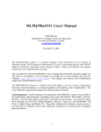
Editing the File Header
A header accompanies each data file and describes the setup of the radar system at the time of data
collection. Some of this information can be edited to correspond to post-processing changes or for report
generation. Also, the file header should include field information such as location, client, date, job
number, surface material, or other information useful in characterizing a site.
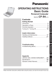
Figure 1: Edit File Header Dialog Box.
File header parameters include: file name, antenna frequency, range, transmitted pulse position, channel,
samples/scan, bits/sample, scans/unit, units/mark, dielectric constant, and approximate depth range.
Scans/unit will be English (Imperial) or Metric units depending on what linear units you selected in
View>Customize.
1
To open the file header choose Edit > File Header or by select the
2
Review and change as necessary the following information in the file header: Position (ns),
ft/mark, scans/meter and dielectric constant.
3
button on the Toolbar.
•
The scans/sec, ft/mark, and Range should be known parameters from the survey, and the
scans/meter will have to be estimated if the data was not collected with a survey wheel
•
Use the Position parameter to shift the time-zero of the vertical scale up or down. For
example, to align it with the ground surface/top of the time window.
•
Dielectric constant values vary from material to material. The value you enter for the
dielectric constant will define the vertical depth scale. Selection of the proper value of this is
very important to obtain reasonable depth estimates of subsurface features. For a complete
discussion, refer to Appendix B. The Depth parameter, if different from 0, will take priority
over the dielectric-based depth scale.
After changes are made, choose the Save button to save any changes that you made to the File
Header.
MN43-171 Rev F
8
Geophysical Survey Systems, Inc.
RADAN Manual
Main Module
The grayed-out box in the center contains some of the initial setup information that the GPR system used
to collect data. It also keeps a running track of any post-processing steps done in RADAN. Also, if you
used a GPS with a SIR-3000, the GPS coordinate information is stored here in two parts: Starting GPS
Info and Ending GPS Info.
GPS Entry Explained
GPR Tick Count: This is an internal system time clock. It can be ignored.
Latitude: This is a coordinate either North or South of the Equator. The first two digits are degrees. The
remaining digits are minutes.
Longitude: This is a coordinate either East or West of the Prime Meridian. The first two digits are
degrees. The remaining digits are minutes.
Altitude: This is the height of the GPS receiver in meters above sea level.
UTC: This is a Universal Time Count that the GPS is receiving from the satellite. The format is
hours/minutes/seconds, or hhmmss.ss
Data Display Options
Radar data can be displayed in five different formats:
Linescan : In the Linescan format your data is displayed in a color-amplitude form, and a color is
assigned to a specific positive or negative amplitude value of the recorded signal, depending upon the
color table and color transform selected. The vertical scale represents time (or depth) while the horizontal
scale represents the horizontal distance traveled by the radar antenna. The Linescan display is the most
useful for mapping man-made objects, such as underground storage tanks, pipes, and drums.
Wiggle : In the Wiggle format the data, consisting of multiple radar scans, are displayed as waveforms
or “wiggle traces.” Wiggle plots are more useful for identifying geologic features, such as a clay layer or
a water table. In both formats, the whole data file is displayed, with time zero (beginning of each scan) on
top and time (or depth) increasing downward.
O-Scope : In the O-Scope format, you are able to view your data one scan at a time and as an
individual waveform or wiggle trace. In O-Scope, time zero is at the left of the display, with time (or
depth) increasing to the right.
Linescan with Wiggle : In the Linescan with wiggle format your data is displayed in the Color
amplitude form as described above with the addition of a Vertical wiggle trace display that appears on the
right hand margin of the active file. Display Gains and Transfer Functions can be applied separately to
either the Linescan display or the Wiggle trace display.
The trace that appears in the wiggle trace window will scroll automatically when the display cursor is
placed in the linescan window and the Left mouse button is clicked on the display.
MN43-171 Rev F
9
Geophysical Survey Systems, Inc.
RADAN Manual
Main Module
3D Display : The 3D display is only active if you have purchased the 3D QuickDraw module for
RADAN. The 3D Display allows you to view 3D files or to view a single profile in 3D and use the 3D
display tools to analyze it.
•
Once a file has been opened in one of the formats by selecting the appropriate toolbar button
or View drop down menu display, it can be closed by clicking on that toolbar button again,
providing that at least one view remains active.
•
If a file is open in a format and you wish to see it in a different format, simply click on the
appropriate button. The new display will not preserve any display gain that you applied to the
profile. You will need to reapply display gain.
•
For a detailed analysis of a radar wavelet, open both the Linescan and O-Scope views for the
file.). Move the two views so they are visible, either manually or by using the tile function
(under Window > Tile > Vertical or Horizontal view) and click on the Linescan view at the
point of interest. Note that the O-Scope view will display the corresponding scan number.
This is a good way to correlate waveform attributes with features found in the Linescan
representation. (See also Linescan with Wiggle display). You can also display gain the scan
wave as well as the linescan image.
Note: A display format is active when the button is in a lighter background in comparison to its
disabled state. One of the three display buttons must be active at all times. It is impossible to disable all
three.
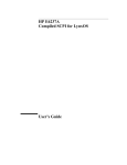
Display Parameters Setup
The Display Options command under the View menu allows you to review and modify the display
parameters for your data. There are four icons for the different display formats: Linescan, Wiggle, OScope, and 3-D (available only with the 3D option) as well as the Print icon.
Double-click on a display format icon to open the Parameters dialog box for the selected format.
Figure 2: Display Parameters Setup dialog box.
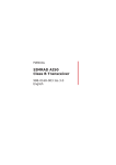
Linescan Display Parameters
Select the Linescan
icon on the toolbar to create a color-amplitude image of the data file as it is
loaded. The Linescan Parameters dialog box (Figure 3) can be opened by selecting the Linescan icon in
Display Parameters Setup.
MN43-171 Rev F
10
Geophysical Survey Systems, Inc.
RADAN Manual
Main Module
Figure 3: Linescan Parameters Setup dialog box.
Color Table: Color is used to code the amplitude of each scan (i.e., the recorded radar signal) as shown
in Figure 3. You may choose one of the standard display color tables from a list of twenty-five tables. A
color table represents the amplitude of the recorded radar signal mapped to different colors.
For instance, white in color table 1 corresponds to the highest positive amplitude pulse; therefore, when it
appears on the radar record, it means that there is a strong reflection (or a high dielectric contrast).
•
Generally, dark means low amplitude signal. Therefore, a large black region on the linescan
plot could be indicative of a uniform structure (such as a homogeneous sand deposit) with
little or no dielectric contrast.
•
The first eight color tables are preset.
•
Tables 9 - 16 may be customized.
•
Tables 17, 18, and 19 are high-resolution (256 shades) gray scales.
•
Tables 20-25 are high-resolution 256 shade 2-color tables.
RADAN defaults to Color Table 17.
Color Transform: You can also change the Color Transform to enhance weak amplitude or small
contrast reflectors. The color transform determines whether the color scale applied to the radar wave’s
amplitude is linear, logarithmic, exponential, or customized. This function can also be used to deemphasize certain features.
•
For example, in a logarithmic map, all low amplitude signals are assigned into a compressed
lower color range, and the range of high amplitude signals is extended.
•
If white represents a high-amplitude signal, then there will be more white area for a given
data set than in a linear transform.
•
There are 16 color transforms (transforms 9 - 16 may be customized), with the default being
linear (Color Transform = 1).
In addition, a Wiggle display may be superimposed onto the Linescan plot by checking the Wiggle Over
Scan box.
MN43-171 Rev F
11
Geophysical Survey Systems, Inc.
RADAN Manual
Main Module
Note: Care must be taken when selecting wiggle parameters for the Wiggle Over Scan, because the
wiggle trace may obscure certain color table transform combinations.
Wiggle Display Parameters
Wiggle format is used to create a wiggle trace representation of the data as it is loaded into RADAN.
Again, the vertical axis corresponds to the time (or depth) while the horizontal scale represents the
distance traveled with the antenna. You may choose for presentation purposes to vary the wiggle trace
parameters.
Figure 4 shows the Wiggle Parameters dialog box that can be found by selecting the Wiggle icon in the
Display Parameters Setup.
Figure 4: Wiggle Parameters dialog box.
Scale: Determines the relative amplitude of the wiggle trace.
Space: Determines the relative spacing between wiggle traces.
Stack: Averages several scans and presents the results as one wiggle trace. In a strict sense this is not true
stacking because the antenna may have been moving, thereby averaging out features as well as random
noise.
Skip: Determines the number of scans to omit between wiggle traces. Unless otherwise specified, this
value will be zero.
Fill: Determines how much (Level (%)), if any, as well as the polarity of pulses (Criteria) that are filled.
•
You may choose to fill either the Positive or Negative pulses, Both, or None.
•
You may choose the fill color by clicking on the color palette and the wiggle trace width
using the Line Width option.
Chop: Zeroes out either the positive or negative side of the return radar signal. It defaults to None.
MN43-171 Rev F
12
Geophysical Survey Systems, Inc.
RADAN Manual
Main Module
O-Scope Display Parameters
O-Scope display represents an oscilloscope trace of one scan of radar data in a file and is configured by
pressing the O-Scope icon on the Display Parameters Setup (see Figure 5). The scan number is displayed
below the trace, and the entire radar file may be viewed in this format by pressing scroll right or scroll
left. (You can use the Stop Processing
data window to scroll at a slower rate.)
button to stop scrolling, or, you can use the scroll keys in the
Figure 5: O-Scope Parameters Setup dialog box.
Scale: Determines the relative amplitude of the wiggle trace.
Stack: Averages several scans and presents the averaged results as one wiggle trace. In a strict sense this
is not true stacking because the antenna can be moving, thereby averaging out features as well as random
noise.
Fill: Determines how much (Level (%)), if any, as well as the polarity of pulses (Criteria) that are filled.
•
You may choose to fill either the Positive or Negative pulses, Both or None.
•
You may choose the fill color by clicking on the color palette and the oscilloscope trace
width using the Line Width option.
Other Display Options
The user may also choose to change the display using General Parameters in the Display Parameters
dialog box (Figure 2).
Start/End Sample: RADAN allows you to enter the start sample (default 1) and end sample (default 512
or 1024) to show the portion of each scan that interests you. For example, if the data is recorded at 1024
samples per scan, but most of the important information is located between sample 1 and 512, you may
enter an End sample of 512 to show only the upper half of your data. Essentially, this expands the vertical
scale of your data by a factor of 2.
Also, if you have a large data file and you are interested in viewing an object located in the middle of the
file, you may change the Start Scan and End Scan so that only that portion of the file is displayed.
Display Scale: Allows you to display the position scale along the horizontal axis. Vertical grid can be
displayed by selecting the Display Grid option.
MN43-171 Rev F
13
Geophysical Survey Systems, Inc.
RADAN Manual
Main Module
Display Parameters Dialog Box: Allows the user to change how the markers are displayed. Click on
the Marks option to display Short or Long marks; select None if you do not want any marks displayed on
your data.
Channel: For SIR-20, PathFinder, SIR-10, SIR-10A, SIR-10B and SIR-10H users, the Channel option
allows you to display all multi-channel data simultaneously or one channel at a time.
Save: Allows you to save your favorite display setting for Recall at another time. To save changes as a
new user parameter file, click Save and choose a name. The new pam file will be stored in your output
directory. To make any changes permanent, click Save and browse for the RADAN XP program
directory. You will see a RADAN.PAM file there. Overwrite that file with your new pam file and call it
RADAN.PAM. Changes are now permanent. See also: RADAN File Types (.pam files).
Interactive Display
The main data display window of RADAN is designed so that different menus and functions can be
accessed by right-clicking at particular places. (right mouse button functionality): Key features and
functions of the RADAN interactive display are summarized in Figure 6.
Certain functions can be accessed by clicking the right mouse button with the mouse cursor in the data
window or within the gray vertical scale area in any display format. This shows small menu boxes that
provide a fast access to some functions also available in the main menu or on the toolbar (Gain, Select,
Horizontal and Vertical Units, Color Table, and Color Transform selection). The user may choose to
display the horizontal scale in distance units or scan number, or the vertical scale as time, depth or sample
number. They also allow the user to display a frequency spectrum of data (see Frequency Spectrum of
Data).
The menu options are slightly different in each display format. For example, only the horizontal scale
parameters can be modified in O-Scope format; the Color Table and Color Transform only apply to the
Linescan display, etc. Depth and Distance/Scale options are active only if the necessary parameters
(dielectric constant and Scans/Unit value, respectively) are entered in the file header.
Dragging the vertical split bar (left edge of the data window) to the right or left allows you to display or
hide the vertical scale. The horizontal split bar at the bottom of the data window splits the data window in
two. Each of them may then be modified separately using the same interactive tools.
The name of any current Region will also be displayed next to coordinate info on the status bar.
Note: Cursor position boxes at the bottom of the RADAN main data display window are also affected
by the display format, selected units, and data window content. These appear in the Status Bar. In order to
view them, make sure that the Status Bar is checked under the View menu.
MN43-171 Rev F
14
Geophysical Survey Systems, Inc.
RADAN Manual
Main Module
Interactive Display Options
Figure 6: Interactive display options (Linescan format).
MN43-171 Rev F
15
Geophysical Survey Systems, Inc.
RADAN Manual
Main Module
Editing the Data
Viewing the Data
To view data use the Left
and Right
scroll arrows located in the Command Toolbar. The scroll
buttons are useful for a quick review of long data files where it is impossible to view the entire file on the
screen at once.
•
These will allow you to scroll continuously towards the beginning (Left arrow) or the end (Right
arrow) of large files.
•
There is a scroll bar at the bottom of the display to show the relative position of the displayed
data within the file
•
Use the Stop Processing
point.
•
Use the scroll arrows in the data window to scroll at a slower rate.
button (located in the Command Toolbar) to stop scrolling at any
Removing Unnecessary Information (Select Block)
You may choose to remove (Cut) unnecessary information from the data file for processing or report
presentation purposes.
1
Choose Edit > Select to selecting a rectangular overlay.
Note: Depending upon how your monitor is configured, the rectangular overlay may be similar
in color to your data file and therefore not be apparent. The overlay will appear at the left of the
file screen. If you are having difficulty seeing the overlay, try changing your color table.
Handles
Select Block
Select Dialog Box
Figure 7: Example1.dzt showing the rectangular Select Block.
(Color Table 25. 256 shade Red, White and Blue)
MN43-171 Rev F
16
Geophysical Survey Systems, Inc.
2
RADAN Manual
Main Module
Next, move and/or adjust the overlay to fit over the section you wish to edit and save as a separate
file or eliminate by clicking on it with the mouse. You can either drag the overlay to move it, or
simply type in sample and scan values for the beginning and end of the overlay.
•
This overlay may be adjusted in both the horizontal and vertical directions. The Select Block
contains tiny squares either centered on each face or located on each corner. These squares
act as handles that can be used to resize the Select Block.
•
You will see within the dialog box the starting and ending scan and sample number that will
tell you the horizontal and vertical limits of the rectangular overlay. You may also move the
entire overlay by placing the cursor within the overlay and dragging the mouse until the
overlay is centered over the section of interest.
Figure 8: Example1.dzt. Showing the edit block moved to the desired location.
3
To remove radar scans at the beginning and end of the file (these occur when the antenna may be
stationary and running in continuous mode), simply align the mouse at the midpoint on the right
side of the overlay. The mouse cursor will change into a left/right arrow symbol when you are in
the right place.
4
Then, drag the mouse until the box is at the desired width.
Stationary antenna positions
Figure 9: Example2.dzt. Stationary antenna positions to be edited.
MN43-171 Rev F
17
Geophysical Survey Systems, Inc.
RADAN Manual
Main Module
Figure 10: Example2.dzt. Select Edit Block positioned over file segment to be saved.
Note: If the overlay or the midpoint box on the right side of the overlay is difficult to see, you
may enter the starting and ending scans corresponding to the overlay’s desired horizontal width.
This display limitation may be overcome in many cases by changing the color table being used.
5
Once you are satisfied with the section you have selected, click OK.
6
Choose Edit > Save or use the Scissors
sections of the file.
button located in the toolbox to remove undesired
•
The cut file action will remove the section of a radar file selected by the mouse-driven
rectangular overlay.
•
RADAN will automatically save the remaining data using a new, user-defined name.
•
If you are not satisfied with the box you have selected or with the edits you have made, you
may choose not to save the new file and all the edits will be undone.
Note: If you make a mistake and cut the wrong section, the edits made to the original file will
be undone if you select Cancel when RADAN goes to save the changes under a new file name.
Saving the Selection in a Separate File
In large data files, you may find it easier and less time consuming to process by saving a small section of
data and process it.
1
Select the desired portion of the file.
2
Choose Edit > Save. You will then be prompted for the new file name under which the new data
will be stored.
Zooming In: Expanding the Vertical Scale of a Data File
The rectangular overlay may be adjusted in the vertical direction as well as horizontal.
1
Choose Edit > Select.
MN43-171 Rev F
18
Geophysical Survey Systems, Inc.
RADAN Manual
Main Module
2
Move the rectangular overlay to the area you wish to enlarge.
3
Use the handles located at the rectangular overlay’s corners and midpoints to shape the rectangle.
As described above, this is accomplished by moving the mouse to the box and dragging the
mouse to expand or contract the overlay to the desired size. Click OK.
4
Next, right click on the data and click Accept Block to cut the selected section and save the
section using a different file name.
5
The selected section, consisting of a specific number of samples will then be resized to the
number of samples in the original file.
•
For instance, if the vertical length of your rectangular overlay is 300 samples long, and your
original data file is a 512-sample file, RADAN will resize the selected section so that it is 512
samples long. The horizontal width of this new file will be determined by the number of
scans selected in the rectangular overlay.
Figure 11: Example1.dzt. Select Edit Block positioned over file segment to be zoomed (1024 samples).
Figure 12: Example1.dzt showing completed edit (Zoomed Section – 1024 samples)
MN43-171 Rev F
19
Geophysical Survey Systems, Inc.
RADAN Manual
Main Module
Working with the Database
RADAN now encodes information in a permanent, storable database based on Microsoft Access. This
means that the database file associated with each .dzt file can be opened and edited in Microsoft Access.
However, Microsoft Access is not required to use the database option in RADAN. The database format is
the Microsoft Access .mdb file. A database is automatically created when a file is opened and is only
properly saved when a file is closed. This means that if RADAN crashes while you have a file open, that
database may be corrupted and RADAN may produce an error the next time that you open that file. That
error will say: “Database apparently corrupted, creating new database.” RADAN will then create the new
.mdb file and you will have lost any changes that you may have made to the old database.
There are two main choices in the database window: Table and Regions. Each discrete 3D dataset may be
preserved as a separate region. This allows easy modification of that single dataset’s display properties
and location information. The Tables sections (3D, GPS, Marker) deal with the overall position
information of the entire dataset. Each Region will refer to the master position information contained in
the Tables section in order to properly locate the data.
The following sections discuss how to edit a specific database table, the different databases available, and
how to relate the regions databases with the tables.
Figure 13 shows the window that pops up after clicking the database icon or going to Edit > Edit
Database.
Figure 13: Database Chooser Window.
Each table or region listed in the database chooser window can be accessed by double-clicking on the
table name. Double-clicking on the table name opens up a spreadsheet-style window containing the
relevant data.
MN43-171 Rev F
20
Geophysical Survey Systems, Inc.
RADAN Manual
Main Module
Pull-Down Menus
File: The only option in the File Menu is Merge Regions. Merged regions cannot be broken up, so it is
advisable to save a copy of the file under a different name prior to merging.
GPS: There are two options available in the menu: Import GPS and 3D GPS Position.
Import GPS: When you open a DZT file, RADAN typically examines the folder that the DZT file came
from to find GPS data that it can apply to the radar file. If it finds a TMF file and a GPS location file
(TXT or PLT) with the same root name as the DZT, it is automatically loaded. If not, RADAN will
prompt you to specify first the TMF and then the location file. It will then save the necessary information
to the GPS table in the database.
3D GPS Position: This dialogue allows you to ascribe GPS coordinates to a 3D dataset. This allows you
to correctly position a 3D area by using coordinate values that were recorded separately from the GPR
data. Two values are needed and one of them must be the local grid origin.
Figure 14: Global GPS Position Dialog
•
Region: If you have a multi region file, this allows you to specify which region’s origin to
use.
•
GPS Units: Either Lat. Long. or UTM.
•
GPS X/Y Origin: This is the GPS coordinate of the grid’s local origin point (0,0).
•
GPS Field X/Y: This is the GPS coordinate value of another location within the grid. The
further away from the origin value, the better.
•
Local Field X/Y Offset: This is the location of the second GPS point (not the origin) within
the grid. The distance units are those set in the View>Customize menu. Think of this as the
coordinate within the grid.
Note: All of the GPS coordinate values for Lat/Long are expressed in decimal degrees. To convert
degrees.minutes.seconds to decimal degrees, divide the minute value by 60, and the second value by 3600
and add to the degrees. For example: a latitude of 42 deg N 46 min 40.26 seconds becomes 42.7778514
degrees. (42 + 46/60 + 40.265/3600)
MN43-171 Rev F
21
Geophysical Survey Systems, Inc.
RADAN Manual
Main Module
Note: This functionality is provided on a trial basis for users of v. 6.6. See page 2 for details.
Video: This menu has one option: Video Sync. This is useful if you are recording digital video at the
same time as GPR data. After syncing with the video timeline, you can display that time in the status bar.
You will still need to view the video data in a separate player. You can synchronize them by specifying a
scan number within the data file, the corresponding time in the video timeline, and the distance offset
between the scan location and the location that the camera is recording.
•
File Scan #: The file scan corresponding to the video synchronization point. Typically this
will be zero.
•
Video Time (sec): The video time corresponding to the File Scan #.
•
Video Pos. Offset (distance): The distance offset between the field of view of the video
camera and the antenna. The distance is positive in the direction of travel. For example: if the
video camera is mounted on the front of the data collection vehicle looking forward 10 ft., the
vehicle length is 20 ft, and the antenna is mounted 5 ft behind the vehicle, then the offset
would be 35 feet.
Note: This functionality is provided on a trial basis for users of v. 6.6. See page 2 for details.
Channel: This menu has one option: Position Reference. This is used to locate the GPR antenna relative
to a GPS receiver. The inline offset is the distance forward (positive) or backward (negative) along the
collection line from the GPS receiver. The crossline offset is the distance to the right (positive) or left
(negative) from the receiver.
The channel position offset is disabled for TerraVision data. TerraVision data is handled in a unique way
when it is loaded into RADAN.
Tables
The RADAN database is structured as a series of “tables.” A “table” can be considered to be a simple
spreadsheet containing a number of columns and rows. Each row in the table is called a “record.” A
record contains a number of properties called “fields.”
As an example of how this all works, consider the marker table associated with a RADAN File. The
marker table contains markers associated with different scans. Each marker is a separate record in the
marker table. The different marker properties such as its scan number and type (distance mark or user
mark) are fields in the marker record. Adding or deleting a marker is simply adding or deleting a record
from the markers table.
The RADAN database is a relational database. This means that information from one table may be related
to information from other tables. The relationships between different tables are described in the following
section.
Each table in the database file can be viewed and edited in the standard spreadsheet format (Figure 15).
MN43-171 Rev F
22
Geophysical Survey Systems, Inc.
RADAN Manual
Main Module
Figure 15: Spreadsheet editing display.
Editing Data
The image above shows the spreadsheet table associated with the markers database table. Different
marker properties can be directly modified by clicking on the column and performing the desired action
whether typing in a value or clicking on a checkbox. Note: None of the edits are saved until the
button is pressed.
Deleting Data
Specific rows of the database are deleted by clicking on the left-most column of the table, which
highlights the entire row, then selecting Edit > Delete from the Edit menu item. Multiple records can be
selected by holding down the “Shift” key while pressing the mouse button on more than one row. These
multiple records can then be deleted using the Edit > Delete menu items. Note: None of the deletes are
button is pressed.
saved until the
Adding Data
New records are added to the database table by typing in the desired information in bottom row. Note:
button is pressed.
None of the added records are saved until the
Some tables require unique information in one or more columns. If duplicate information is typed in, an
error message will pop up. One example of this is the Marker table. There cannot be any duplicate scan
numbers within each region in the Marker Table.
Sorting Data
Clicking a column header sorts the table in an ascending direction based on the values in the column.
Clicking on the same column header twice changes the sort direction. The sort capability is a powerful
tool for quickly finding certain information in large database tables.
MN43-171 Rev F
23
Geophysical Survey Systems, Inc.
RADAN Manual
Main Module
Scroll To Scan Button
The Scroll to Scan button is used to synchronize the linescan data window with the selected scan number
in the database. To force the linescan window to scroll to a specific scan number, first select the desired
record containing the scan number by pressing the left mouse button on the left-most column of the
spreadsheet. This will highlight the entire row. Then, press the
button. In RADAN version
6.0, this option only works with the markers table.
Refresh Button
The Refresh button is used to reload the data in the spreadsheet from the database file. This button is
useful when undesirable edits have been made to the spreadsheet data. Pressing the
button
performs the same task as closing and reopening the table.
Apply Button
The apply button saves all changes made to the spreadsheet to the database file.
Database Tables Descriptions
Marker Table
The Marker table can be accessed via double-clicking on “Marker” in the Database Chooser Window or
by clicking on the Edit Marks button on the main tool bar
or by selecting Edit > Edit Markers from the
RADAN Main menu items. Using any one of the three methods opens up a spreadsheet containing all of
the marker information.
The Marker table shown contains a number of new properties in addition to the properties of markers in
previous versions of RADAN. Each marker property is briefly described below.
Scan: The scan number associated with the marker. This scan number is relative to the scan number
associated with the start of the region in which the scan number belongs. All scan numbers belonging to
region 0 are referenced relative to the beginning of the file.
UserMark: A marker in the data that has been added by the user either during data collection or from
RADAN. This marker may have a name and or position information. User marks appear in line scan
mode as dashed lines.
DistMark: A marker in the data that has been added either automatically during data collection or by the
user in RADAN. DistMarks (which is short for distance marks) that are added automatically during data
collection contain the correct distance values of the corresponding scan. This is a safety feature for GPR
systems that may skip scans when the antenna is moved too fast to maintain the specified scans per
distance interval. The distance normalization process in RADAN uses the distance mark values to
perform interpolation to fill in the missing scans in files.
Distance-based GPR data collected on the SIR-3000 with a GPS receiver attached contains GPS location
information at each distance mark in the GPR data file. In RADAN, this GPS information can be loaded
into the marker table. See section describing the GPS Table for more details.
MarkName: The user-assigned name of the mark. It can be up to 64 characters in length.
X,Y,Z: The x-, y-, and z-coordinates of the scan.
MN43-171 Rev F
24
Geophysical Survey Systems, Inc.
RADAN Manual
Main Module
Profile: The profile line number for 3-D files.
Region: This is the region number in which the marker belongs. This value is not fully implemented. By
default, all scans in all files have the region number “0.” In RADAN the only case where the region
number will be non-zero is where the user has used the Append option in RADAN to create an appended
file.
Zone: This is the UTM zone for markers containing GPS position coordinates.
GPS Table
The GPS table stores GPS data imported from GPS log files. GPS data logged on the SIR-3000 and
TerraVision systems is stored in two files: a TXT or PLT file and a TMF file. GPS data collected with the
SIR-20 is stored in a POS file. See GSSI Technical Note 0101 for details regarding GPS integration with
the SIR-3000. See the SIR-20 manual for GPS integration with that instrument.
The GPS data collected by each system is loaded into the database file from the database table viewing
window. If RADAN detects a TMF and a TXT or a PLT file with the same root name as the DZT file in
the same folder, then it will automatically load GPS information. Otherwise you can load it manually by
accessing the database table window by going to Edit>Edit Database and selecting “GPS” as shown in
Figure 16.
RADAN will also accept NMEA GGA files which are output by most GPS instruments.
It is your responsibility to get the GPS output into the NMEA GGA string. GSSI does not support GPS
instruments. Contact your GPS manufacturer if you are having trouble getting your GPS to output
data in this format.
Once you have a NMEA GGA file with the extension .log or .txt, click import GPS. RADAN will ask you
to select the correct file. Change the Files of Type to “NMEA GGA File (*.Log; *.Txt)” and select the
correct file. RADAN will then parse out the information that it needs.
Figure 16: Procedure for importing GPS data into GPS table.
The GPS table contains the GPS coordinates in UTM coordinate system with respect to the global origin.
The coordinates of the first scan are identical to the global coordinate origin stored in the Regions Table.
All subsequent GPS values are relative to the first scan. The horizontal and vertical units of the UTM
coordinates are specified using the View > Customize > Linear Units option in RADAN. A brief
description of each field in the GPS table is presented below.
MN43-171 Rev F
25
Geophysical Survey Systems, Inc.
RADAN Manual
Main Module
Figure 17: GPS table.
Scan: This is the scan number with respect to the first scan number of the specified region.
X,Y,Z: The x, y, and z coordinates with respect to the global x-, y-, and z- coordinates that are saved in
the Regions Table.
Zone: The UTM zone to which the data are referenced.
Region: This is the local region number in which the scan belongs.
3D Table
The 3D Table contains local 3D coordinates of the scans in each region. The local coordinates of all 3D
files created in RADAN version 6 are stored in this table.
Note: The information in this table is for viewing purposes only in RADAN. Therefore, the contents of
this table should not be modified. In future versions of RADAN, the information from this table will be
extensively utilized.
The concept behind the fields in the 3D table is to assign coordinates to each scan in the data file. To
accomplish this, the data file is divided into the smallest possible piece, the segment. A segment (Seg in
the table) contains a starting scan number, total number of scans, starting (X,Y,Z) coordinates, and vector
X, Y, and Z lengths. Each segment belongs to a profile. In turn, each profile belongs to a region. A
segment may have a radius of curvature (ROC in the table).
A brief description of each field in the 3D table is presented in Figure 18.
Figure 18: 3D Table.
MN43-171 Rev F
26
Geophysical Survey Systems, Inc.
RADAN Manual
Main Module
ScanSt: This is the scan number with respect to the first scan number of the specified region to which the
indicated segment of the profile belongs.
NumScans: Total number of scans comprising the segment.
FileName: Filename from which data comprising the segment originated.
XSt, YSt, ZSt: Starting x-, y- and z- coordinates of the segment.
XLength,YLength,ZLength: Vector lengths in x-, y-, and z-directions from starting scan to ending scan
in segment.
Seg: Segment number of profile. For profiles that only have one segment this number is always zero.
Profile: Profile number within a region.
Region: Region number.
ROC: Radius of curvature of segment. This function is reserved for future versions.
Special Case: Editing the Markers Database
RADAN provides a way to edit markers entered by the user or survey wheel during the field survey.
Before beginning, please make sure that you read the previous section on the database. There are three
different markers used by RADAN:
User Marks: Manually entered during the data collection.
Distance Marks: Written into the data file using a survey wheel or another distance-measuring device.
Combo Marks: Overlays of distance and user marks.
Marks that are created on older analog systems by pressing the marker button on either the antenna or
SIR-3 or SIR-8, have to be manually entered.
Note: Distance (or Combo) markers are needed to perform Distance and Surface Normalization. If you
are converting User marks (from clicking Mark in the field during data collection) to Combo marks, make
sure that the DistMark box next to the appropriate mark is checked. Click Apply to save any changes.
Microsoft Access Database creates a database that can be accessed from one RADAN session to another,
and saved in Microsoft Access format.
1
To edit markers, choose Edit > Edit Markers or click on the Edit Markers
Figure 19: Edit Markers Setup Dialog Box.
MN43-171 Rev F
27
button.
Geophysical Survey Systems, Inc.
2
RADAN Manual
Main Module
Next, you will want to find all the markers you wish to keep (i.e., those that correspond to station
locations which will help orient the data to your survey line or grid). Set the Horizontal Scale on
your linescan data window to scans. You can do this by right-clicking on the vertical scale bar at
left and finding Scans under the Horizontal Scale section. Next, find the scan number of the mark
you are interested in by left clicking on that mark. The scan number will be displayed in the
Status Bar at the bottom of the screen.
• If you know the mark location, you can click on it in the Database window and click Scroll to
Scan to have the data window advance to the appropriate mark.
To Delete A Marker
1
Select the marker by left-clicking on the gray box at the far left column of the database window.
This will cause the whole row to be highlighted.
2
Find the Edit pull-down menu at the top left of the database window (not the main set of pulldown menus at the top of the RADAN screen).
3
Select Delete. Be sure that you are deleting the correct mark, because there is no undo delete
option.
To Add A Marker
To manually add a marker, follow these steps:
1
Scroll to the bottom of the marker database window and find the empty row with an * next to it.
2
Click on the Scan window and type in the scan number where you want the marker to go.
3
Type in any additional position information in the appropriate window.
4
Make sure that the correct marker type box (UserMark or DistMark) is checked.
5
Click Apply.
To Manually Change Marker Type
To manually change the type of marker, follow these steps:
1
Find the scan number of the mark that you want to change and find that mark in the database
display.
2
Place a check in the mark type box to change the mark to the desired type. If you want a Combo
mark (a mark that encodes Distance, but still remembers that it is a User-defined mark), make
sure both UserMark and DistMark are checked.
Regions Table Descriptions
Figure 20 shows the three Regions items in the database: Coordinates, Position, Properties. These can be
accessed by double-clicking on them. Additionally, if you would like to merge all of the regions together,
select Edit>Merge Regions. This process cannot be undone.
MN43-171 Rev F
28
Geophysical Survey Systems, Inc.
RADAN Manual
Main Module
Coordinates
Figure 20: Display Coordinates
It is possible to collect data with no positioning device or with multiple positioning devices. The Display
Coordinates control allows you the option of drawing location information from different databases.
Region: Selects which region you will apply changes to.
Source: Selects which type of location information you are using.
•
Survey wheel: This data is drawn from the Marker Table and typically contains only linear
distance information.
•
3D Table: This data is drawn from the 3D Database and allows X,Y positioning of data
points. The 3D database is only populated if the file is a 3D file.
•
Imported GPS : This data is drawn from the GPS data and allows X,Y positioning of data
points. This allows a single profile of GPS collected data to be displayed in 3D.
Type: Selects which display type you would like location information displayed as. It is only possible to
display data in the 3D QuickDraw module if you select X,Y or GPS.
•
Scan: Location is scan number from the beginning of the region. This display type is
available with all collection methods, including time-based continuous mode and point data
collection.
•
Linear Dist.: Distance offset as a straight line from the beginning of the region in units
selected under View>Customize. This is only possible with survey wheel or GPS collected
data. This will also disregard any data in the 3D database with the result that the region will
show as a single profile in the 3D display mode. This display type is useful for single profiles
of data.
•
(X,Y): If you have 3D or GPS data, then each point has both an X and a Y coordinate used to
locate it in space. This choice will display that information and make it possible to view the
data as a 3D area in the 3D display mode.
•
Ratio: This type will display a ratio of your current location to the whole data file length.
Reference: This sets the zero point that your data is offset from.
•
Local will establish an arbitrary zero position that your data coordinates will be referenced to.
Usually this is either the start of your profile line or the 0,0 origin of the 3D grid.
•
Global is used mainly when you have a GPS. This sets a GPS coordinate at the reference
point and all data points are offset from that spot.
MN43-171 Rev F
29
Geophysical Survey Systems, Inc.
RADAN Manual
Main Module
Position
Figure 21: Region Position
The Region Position item allows you to manipulate the position of each region.
Region: Selects the region to apply changes to.
Rotation Angle: This will rotate the region around the local X,Y origin. Values entered here are degrees
in a counter-clockwise direction.
Local X/Y Origin: This is the coordinate within the single region that will be considered its origin for the
purposes of rotation and concatenation with other regions.
Global X/Y Origin: This origin is typically used only with GPS data to place the region against a
Lat/Long coordinate system.
Flip Vertically/Horizontally: Checking these boxes will flip the region in the desired direction.
Properties
Figure 22: Region Properties
The Region Properties item allows you to change region name. It will also display the starting scan
number or the currently selected region and the total number of scans in that region.
MN43-171 Rev F
30
Geophysical Survey Systems, Inc.
RADAN Manual
Main Module
Generating Displays for Reports
GPR data displays can be simplified so that significant features stand out. Changing or customizing Color
Tables and/or Color Transforms can be used to emphasize the amplitude ranges of specific features. For
example, if you are trying to image weak reflections like fine soil layering, you might choose Color Table
1, Color Transform 3. This shows a lot of color variation around zero amplitude and can help to make
weak reflections more visible.
In addition, the size of files can be tailored to fit onto a report page using RADAN’s file editing feature
found under the Edit menu.
1
Select the desired portion of the file.
2
Use the Cut command (or select the Scissors button from the toolbar) to remove the desired
section.
3
You will then be prompted for the new file name under which the new data will be stored.
Note: It is easy to export data using RADAN via the Windows clipboard to annotate using other
drawing programs. You may copy a selected section, paste it to the clipboard and export it to other
programs, such as CorelDraw, Adobe Photoshop, or Microsoft Word. Simply click the clipboard icon
on the toolbar, open the target application, and paste it into that program. You can also use the Print
Screen key to save the active window of the screen. This can now be viewed and edited in MS Paint.
Printing a File
Once a file has been edited and processed, you may choose to print this file for publication. The Print
command, found under the File menu is used to print a file as well as all the header and processing
button can also be used. The print format (Linescan, Wiggle
information that goes with it. The Printer
or O-scope) will be the same as that of the active window.
1
Choose File > Print Setup to select or establish the default printer.
2
Select the printer port (usually LPT1). The Setup option will also allow you to select the paper
size, source and orientation (portrait or landscape).
3
Preview your print file by using the Print Preview command (found under the File menu), which
will display the active file as it would appear when printed.
•
Print Preview allows you to view either one or two pages at a time, move back and forth
through the document, zoom in, zoom out and initiate printing. The next page and previous
page commands may also be used to scroll through the pages in the print preview.
Note: In the Print Preview, your file may appear too stretched or too compressed horizontally.
To adjust scans per inch for printing purposes go to Display Parameters option under View, or on
the main tool bar. Scroll to and select the print option on right side of the display box. Set the
desired number of scans per inch. Check on final print resolution through Print Preview.
4
When satisfied with what you see on the screen, click Print or select Print from the File menu.
MN43-171 Rev F
31
Geophysical Survey Systems, Inc.
RADAN Manual
Main Module
Note: Some printers have different dots per inch resolution. Select Printer Zoom found in the
View menu under Display Options, and enter a number between 1 and 5, depending upon
whether your printer is a laser or an ink jet.
•
In some cases, the size of the RADAN file to be printed will exceed the internal memory
capacity of the printer spooled for use. You should be aware of the memory size of the printer
you are using and the size of the file they are trying to print. If the file size exceeds the printer
memory size, Windows will return a printer error message. You should then cut the file into
smaller sections and print them individually.
Saving Your Data
We recommend storing your output files in a separate output directory to assure that the raw field data
and processed data are not stored in the same folder and risk being over-written or otherwise corrupted.
Saving to Hard Drive
Saving data in C:\...\RADANOUT or some other exclusive folder will help prevent accidental deletions.
Along the way, as data are edited, filtered, and processed, RADAN will automatically ask you for a new
file name so it may store the updates without overwriting old (raw) data.
RADAN will also ask you if you intentionally want to overwrite a data file. You may save your data in
RADAN data format as a *.dzt file by going to the File menu and selecting the Save As function. You
may choose to save your data using another file name, or on a different drive.
To save FILE1.DZT on Drive A, for instance, go to the File menu and select the Save As function. A
dialog box will appear and you may enter either the file name or drive under which you want your data
stored. In this case, you will either type in A:\file1.dzt or select the drive using the mouse.
Data may also be saved using the SEG-Y format. From the Save As dialog box, select SEGY File under
Save as Type. Data will be saved under the SEG-Y format (*.SGY) so that it may be imported into
another processing package. Regardless of which format you choose to save your data, we recommend
that you save all active files before closing them and exiting RADAN.
Note: You may use WinZIP or other archiving programs to compress data files and minimize disk
space. Compressed files must first be decompressed to run in RADAN.
MN43-171 Rev F
32
Geophysical Survey Systems, Inc.
RADAN Manual
Main Module
Chapter 3: Processing
Specific Processing Objectives
You may choose to apply further processing as appropriate, from the Process menu to clarify the GPR
data presentation:
Horizontal and Vertical Filters
Spatial 2D Filtering
Range Gain
Restore Gain
Surface Position Adjustment
Distance Normalization
Horizontal Scaling
Horizontal Distance Adjustment
Deconvolution and Migration
Hilbert Transform
Surface Normalization
Velocity Analysis
These processing functions are described in detail below. Initially, single files are processed step by step.
Once processing parameters have been established for a specified function, you may start processing by
selecting OK in the menu corresponding to the processing function of interest. Use the Stop Processing
button (located in the toolbar) to stop processing at any point.
Once you are satisfied with the processing steps necessary to produce a good-looking data file, a macro
program may also be created to automatically process a data file. Large data sets may be automatically
processed by using RADAN Project Mode. The user assigns numerous data files, all of which are
processed using the steps outlined in the specified macro program. Chapter 6 will discuss in detail how to
create macro programs and process large data sets.
Listed below are specific radar data processing objectives and the methods that will accomplish each of
them. Also included are the critical processing parameters that must be established.
MN43-171 Rev F
33
Geophysical Survey Systems, Inc.
RADAN Manual
Main Module
OBJECTIVE
METHODS
•
Horizontal High Pass Filter
•
Vertical High Pass Filter
•
Spatial Filter
•
Background Removal
•
Vertical Low Pass Filter
•
Horizontal Low Pass Filter
•
Spatial Filter
Ringing Multiples
•
Deconvolution
Remove diffraction (compress hyperbolas)
and correct dipping layers
•
Migration
Increasing visibility of low amplitude
features
•
Arithmetic Functions
•
Display and Range Gain
Detect subtle features
•
Hilbert Magnitude Transform
•
Spatial Filter
•
Arithmetic Functions
•
Local peaks
•
Static corrections
Remove flat-lying ringing system noise
High frequency noise (i.e., snow)
Generate clearer data displays for reports
Table 1: Processing objectives and corresponding methods.
Horizontal Scale Adjustments
Distance Normalization
Distance Normalization allows you to establish a constant horizontal scale between marks. This function
performs rubber-sheeting so that there is an equal distance, or equal number of scans per unit distance,
between markers.
This is generally required when data is collected in continuous mode without a survey wheel and is due to
unavoidable inconsistencies in antenna towing speed. When Combo or Distance Marks are set and
verified (see Editing the Markers in Chapter 2), Distance Normalization will correct the number of scans
between markers by stretching and skipping, thereby correcting for variations in survey speed.
MN43-171 Rev F
34
Geophysical Survey Systems, Inc.
RADAN Manual
Main Module
Figure 23: Distance Normalization Parameters Setup (with meters selected as linear units).
Note: Distance Normalization requires that marker information be stored in the Microsoft Access
Database; otherwise it will be inactive.
Note: Distance Normalization will be “grayed out” and inactive if the file is a 3D file or has GPS
information.
•
Distance Normalization requires a minimum of TWO markers to work.
•
Make sure that the markers are correct (no double or missing markers, first and last markers are
present, all User markers are converted to Distance or Combo) before running Distance
Normalization.
•
The Scans per Unit and the Units per Mark must be assigned a value in the input file header in
order for Distance Normalization to work.
•
Units per Mark are determined at the time of the survey.
•
Scans per Unit may be estimated by using the mouse cursor to count the number of scans between
markers or by taking the Scans/Sec value in the header and estimating the number of seconds it
took to traverse the distance between marker stations.
•
Both Scans per Unit and Units per Mark parameters can be changed for the output file.
•
Horizontal and vertical units (meters, feet, etc.) must be set before opening the file. Use the
Linear Units tab under the Customize command in View menu.
To use, correctly set the scans/unit distance and the distance/mark in the File Header. Then click on the
Distance Normalization button, or Process>Distance Norm. Make sure that the correct parameters appear
in the Distance Normalization window, check the “Apply to User Marks” box, and click OK. Save the file
with a new name when prompted.
MN43-171 Rev F
35
Geophysical Survey Systems, Inc.
RADAN Manual
Main Module
Note the correct values for the scans/unit distance and marks/unit distance in
both the file header and Distance Normalization dialog box.
Figure 24: Example2.dzt. Distance normalization complete. Note the slight shift of the
markers relative to reflectors in the data. Note also that data up to the first mark (scan 22)
has been cut off by the normalization process.
Horizontal Scaling
Data may be modified by adjusting the Horizontal Scale using the Stacking, Skipping and Stretching
button or go to the Process menu and select Horizontal Scale.
functions. To do this, use the
MN43-171 Rev F
36
Geophysical Survey Systems, Inc.
RADAN Manual
Main Module
Figure 25: Horizontal Scaling Parameters Dialog Box.
Note that you can only run one of the three choices at a time. You must click on the circle next to your
desired choice to select it.
Stacking: Select Stacking to apply a simple running-average to stack the data. Stacking combines the
adjacent selected radar scans and outputs a single scan. When stacking values are used in RADAN, the
program will retain the marks in the file. However, the scans per unit distance and marks per unit distance
will be changed in the header. For example if you had a raw file with 80 scans per meter and 1 meter per
mark and you stacked by a factor of two (2) the output file would have 40 scans per meter written into the
header (reduced by a factor of 2).
Skipping: Select Skipping to specify the number of scans you wish to skip over from the previous scan.
For instance, enter 1 if you wish to omit every other scan from the file (hence compressing it by a factor
of 2).
Stretching: Select Stretching to expand the horizontal scale. The Stretching function will calculate the
simple average of two adjacent scans (or the specified number of scans) and place the averaged scan in
between the existing scans.
Figure 26: Example2.dzt. Data file STRETCHED by a factor of 2.
MN43-171 Rev F
37
Geophysical Survey Systems, Inc.
RADAN Manual
Main Module
Appending Files
In some cases it is necessary to collect profiles in segments due either to logistical or data file size
constraints. In order to append two (2) or more segments of the same profile together the user must first
determine if any data editing functions (Marks conversion, Horizontal scaling, etc.) need to be performed
on the data.
In the example that follows we will:
•
Append the file segments,
•
Edit the markers and the file,
•
Perform a Zero Position correction and then;
•
Perform a Surface Normalization.
***In this example we will actually skip a step, as it is generally desirable to perform any signal
processing (Filtering, Migration, Gain functions, etc) on the whole file PRIOR to Surface Normalization.
We will return to this file later on in the manual.
Appended files will be preserved as different regions. This is especially helpful if the files are 3D files.
1
To append files segments together select File > Append File. This opens the Select Single
Channel File dialog box (Figure 27).
Extraneous USER marks
to be removed
‘Hinge’ of Profile 3a and 3b
Figure 27: Example3a and 3b. 40 MHz antenna. Top profile (Example 3a.dzt) is the first segment.
The bottom profile (Example3b.dzt) is to be appended to Example3a.dzt.
MN43-171 Rev F
38
Geophysical Survey Systems, Inc.
RADAN Manual
Main Module
Figure 28: Select Single Channel File dialog box open. First profile segment selected.
2
Select each file segment IN SEQUENCE and select Add from the dialog box. In Figure 28 the
first file segment has been selected.
3
When both file segments have been selected and Added to the Files In Project box, click Done.
4
The files will then be appended. Save the file with a new file name.
Figure 29: All file segments to be appended are Selected.
‘Hinge’ of Example 3a and Example 3b
Figure 30: Example3a & 3b. File append is complete.
MN43-171 Rev F
39
Geophysical Survey Systems, Inc.
RADAN Manual
Main Module
Vertical Scale Adjustments
Surface Position Adjustments
Sometimes it is necessary to vertically adjust the position of the whole profile in the data window (adjust
time-zero). You may want the first positive peak of the direct wave from a ground coupled, bistatic
antenna to be centered at the top edge of the screen so that you can consider ground surface to be at the
top of the window (at Time Zero). This can be done using the Correct Position command in the Process
menu or by selecting the
button. A corrected 0-position will give you a more accurate depth
calculation because it sets the top of the scan to a close approximation of the ground surface.
Figure 31: Position Setup Dialog Box.
In the dialog box, the position of the beginning of the trace on the time scale can be entered.
•
The trace can also be shifted in small increments using the Delta Pos (nS) arrows.
•
The scan to be displayed is selected in the Scan box and can be changed by placing the mouse
cursor on the Display (Linescan, Wiggle, O-scope) and scrolling through the file.
•
When you are satisfied with the correction select OK. The position correction will then be applied
to the entire file. The correct 0-position is usually about 90% of the way to the first positive peak.
•
If you wish to reset the top of the vertical scale to zero, then go to Edit>File Header and replace
the value in Position(nS) with a zero.
Note: To shift the vertical scale without shifting scans in the display, modify the Position parameter in
the file header.
MN43-171 Rev F
40
Geophysical Survey Systems, Inc.
RADAN Manual
Main Module
Figure 32: Example3a&b.dzt. Position Setup dialog box open.
Trace location corresponds to the dashed User mark in the middle of the profile.
Note corrected position of surface reflection
Figure 33: Example3a&3b.dzt. Zero position corrected.
Surface Normalization (Adjusting for Elevation Changes)
Surface Normalization allows you to assign an elevation to the markers in the database and correct for
elevation changes. In other words, Surface Normalization adjusts the vertical scale to remove topographic
effects, which results in horizontal or near horizontal reflectors appearing as they are in reality. For
instance, the water table may appear to have significantly greater relief in radar data than in actuality.
Surface Normalization corrects for the topography and displays the water table as a flat reflector.
Vertical Scale: The Vertical Scale may be set to 1:1 (normal view), 1:2, or 1:4. Using the latter two
scales compresses the vertical axis (and adjusts the vertical scale accordingly) by factors of 2 and 4,
respectively.
This compression of the vertical scale may be necessary if the relative change in elevation for the file is
greater than the display range of the monitor being used. If data is not compressed, the file may ‘run-off’
the top or the bottom of the display window.
MN43-171 Rev F
41
Geophysical Survey Systems, Inc.
RADAN Manual
Main Module
Figure 34: Surface Normalization Parameters Setup.
Normal Level: Normal Level can be manually input if the Auto Level option is deactivated. Surface
Normalization requires that Combo (or Distance) Markers be used.
Note: Elevation values have to be manually assigned to the markers using Edit Markers (see Chapter 2,
Editing Markers.)
When entered, elevation data will be stored in the Microsoft Access Database file.
Figure 35: Example3ab.dzt. All DISTANCE markers converted to COMBO marks and Elevations entered. (See Table
3 for elevations.)
Figure 36: Example3a&b.dzt. Data has been normalized with Auto Level ON, Vertical Scale is 1:1.
Note that part of the file has ‘run-off’ the display window. You must either set a greater Vertical Compression or
change the Auto Level.
MN43-171 Rev F
42
Geophysical Survey Systems, Inc.
RADAN Manual
Main Module
Figure 37: Example 3a&b.dzt. File has been normalized with Auto level set to 92. Vertical Scale is 1:1. Note that by
using an Auto Level value of 92 (top of display window is 92 M) , the highest point (91m msl) in the data will
appear on the screen. Please note that the Vertical scale is set in TIME, not depth (or elevation)
Figure 38: Example3ab.dzt. Auto Level selected. Vertical Scale 1:2. Due to the long time range
of this file a 1:2 compression is probably not suitable for display or printing purposes.
Figure 39: Example 3ab.dzt. Auto Level = 92, Vertical Scale 1:1. While the bottom of this file is missing
(at the lowest surface elevations) .
MN43-171 Rev F
43
Geophysical Survey Systems, Inc.
RADAN Manual
Main Module
About Filters
There are three types of filters available in RADAN to process radar data:
•
Infinite Impulse Response (IIR) filters
•
Finite Impulse Response (FIR) filters
•
2-D spatial FFT filters (F-K filters).
IIR Filters
IIR filters were introduced before the advent of computers, when simple LRC circuits were used as
analog filters. When an IIR filter encounters a feature in the radar data, it produces an output that decays
exponentially towards zero but never reaches it, hence the name “infinite.” IIR filters are not necessarily
symmetrical and while they achieve excellent amplitude response, their phase response is non-linear and
so they can cause slight phase shifts in the data.
Figure 40: IIR Filter Parameters Setup.
•
The IIR Filter Parameters Box lets you define the high and low pass horizontal and vertical filters
as well as the time interval that will be processed, defined by the start and end sample number
(RADAN automatically defaults to the whole time window).
•
The cutoff frequencies are defined in number of scans horizontally and in MHz vertically.
•
You can apply any combination of vertical filters simultaneously and see the result using the
Apply button.
•
Horizontal filters, due to their implementation, will not work under Apply. Select OK to see the
horizontal filter’s effect on the file.
•
When you’re satisfied with the results, Save the processed file.
RADAN uses IIR filters having only one pole so that there is not a sharp break at the cutoff frequency,
which may provide limited noise reduction. As a consequence of this, it may be beneficial to run the same
filter more than once. Or, another approach is to modify the Color Transform (under the Display
Parameters Dialog Box) to hide what little noise remains in your data.
MN43-171 Rev F
44
Geophysical Survey Systems, Inc.
RADAN Manual
Main Module
FIR Filters
RADAN contains Vertical and Horizontal FIR filters as well as Spatial 2-D filters. FIR filters
have a
finite-duration impulse response. FIR filters, when encountering a feature in the data, are guaranteed to
output a finite filtered version of that feature. This property makes it possible to design filters that are
perfectly symmetrical and have linear phase characteristics.
FIR filters will therefore produce symmetrical results so reflections will not be shifted in time or position.
Note, because of the symmetrical nature of FIR filters, FIR filter lengths should always be an odd
number. Generally, FIR filters are normally preferred in digital signal post processing; however, users
more familiar with IIR filters might choose to use them instead.
There are two types of FIR filters available in RADAN, Boxcar and Triangular Filters.
Boxcar Filter: The Boxcar filter is a rectangular window function that performs a simple running
average on the data. A portion of the data, determined by the filter length, is averaged, and the average is
output as a single point at the center of the active portion of the filter window. The filter moves on to the
next sample and the process is repeated. The Boxcar filter assigns equal weight to the data all along the
filter length.
Triangular Filter: The Triangular filter emphasizes the center of the filter more heavily than the ends of
the filter. This type of filter is a weighted moving average, with the weighting function shaped like a
triangle. A portion of the data, determined by the filter length, is multiplied and summed by this function.
The result is output at the center of the triangle. The filter then advances one sample and the process
repeats.
Because of the number of calculations involved, Triangular filters are slower than Boxcar filters. Hence,
we recommend using the Boxcar filter first because of its speed. If results are not adequate try the
Triangular filters.
Data Filtering
Frequency Spectrum of Data
You may wish to determine the predominant frequencies of your data for processing purposes, or to
determine the frequency of any noise. In RADAN, you can display the frequency spectrum of your data in
any display format. The frequency spectrum can be analyzed in detail on a scan-by-scan basis using the
O-Scope display format.
1
Enable the O-Scope display by using the toolbar or View menu. You will see the oscilloscope
representation of a scan (amplitude versus time or depth).
•
2
Use the scroll bar to choose the desired scan. Its number will be displayed beside the cursor
position in the bottom of the main window.
Place the cursor within the data window and click the right mouse button.
•
In the menu box that appears, choose Transfer > Spectrum. The displayed scan will be
replaced with its frequency spectrum plotted in terms of relative amplitude (0 to 1) versus
frequency in MHz.
•
It is recommended to create a Split Display first by using the Horizontal Split Bar, and then
display the spectrum in one of the windows with the right mouse button (Figure 41). This
way, both the waveform and the frequency spectrum for the selected scan will be shown.
MN43-171 Rev F
45
Geophysical Survey Systems, Inc.
3
4
RADAN Manual
Main Module
Move the mouse cursor to determine amplitude or frequency parameters.
•
If you click the left mouse button within the time-amplitude plot, the cursor position display
at the bottom right of the main window will give you values for amplitude and time (or depth
if it is selected as the vertical scale option and a dielectric constant or depth range is input
into the file header).
•
Frequency (MHz) and relative amplitude will be displayed if you click within the frequency
spectrum plot.
Use the Scroll bars to view other scans.
Figure 41: Example 2.dzt. Split Display with Linescan and O-Scope. O-scope display split to show frequency
spectrum of scan 201 on top and scan on bottom. Trace location corresponds to black highlighted marker in the
middle of linescan display.
Horizontal noise
to be removed
Figure 42: Example3a&b.dzt. Upper profile is raw data. Bottom profile has had
FIR Background Removal filter, Ν =1023 applied from sample 20-512 and was then migrated.
A display gain of 2 has been applied to the processed file.
MN43-171 Rev F
46
Geophysical Survey Systems, Inc.
RADAN Manual
Main Module
Figure 43: Split Display with a frequency spectrum in Wiggle format (top) and Linescan Format (bottom).
In the split display, if you use the scroll bar associated with the O-Scope plot, the frequency spectrum
below will be synched to the current scan. Scrolling is not synchronized if you use the scroll keys from
the frequency plot. It is also possible to synchronize to the Linescan plot by clicking on a single scan in
the Linescan display window.
In RADAN, the frequency spectrum can be displayed in the Linescan and Wiggle formats as well, using
the above procedure in the corresponding data windows. This option allows you to analyze frequency
variations along the survey line.
•
In the Linescan format, the scans will be replaced with their frequency spectra. The same color
table will be used. Right-click on the data window, select Transfer, then Spectrum.
•
In the Wiggle format, the wiggle traces (waveforms) will be replaced with their spectral plots
(Figure 43).
MN43-171 Rev F
47
Geophysical Survey Systems, Inc.
RADAN Manual
Main Module
Some Examples Of Different Filter Applications And Their Effects
Figure 44: Example2.dzt. A Vertical IIR Low and High Pass Filter combination (band-pass).
Upper half of spilt-screen is processed data. Lower half is original (raw) data.
Figure 45: Example2.dzt. A 10 scan IIR Horizontal Low Pass (smoothing) filter applied.
Upper half of split-screen is processed data. Lower half is original (raw) data.
MN43-171 Rev F
48
Geophysical Survey Systems, Inc.
RADAN Manual
Main Module
Note removal of ‘time–constant direct coupling pulse
Figure 46: Example2.dzt. 511-Scan FIR Background Removal (Horizontal High Pass) filter applied. Bottom profile
is raw data upper profile is processed data
Figure 47: Example2.dzt. A Vertical FIR Low and High Pass filter combination (notch) applied.
MN43-171 Rev F
49
Geophysical Survey Systems, Inc.
RADAN Manual
Main Module
Removing Flat-Lying Ringing System Noise
(Vertical HP, FIR Horizontal BM, IIR Horizontal HP)
This type of noise is usually most prevalent when the range is set near the maximum limits for the
antenna. It is characterized by flat-lying or horizontal bands usually of a vertical frequency lower (shown
by wider bands) than that of the real reflections in the data set. This type of noise can obscure or mask
real reflections at greater depths.
Figure 48: Example3.dzt. 400 MHz antenna. Data is predominated by flat-lying horizontal or ‘ringing.’
The O-scope display and spectrum correspond to a trace centered on the right-hand hyperbolic target.
Two utilities are shown here. The shallower target located in the upper left is a 6 inch metallic pipe
buried .8 ft below the surface (ε ~ 24). The target on the right is a gas filled PVC pipe 1.85 ft below the surface.
Both targets are buried in clay under a 4-6 inch thick asphalt pavement.
Horizontal High Pass (Background Removal) Filter
Using the Horizontal High Pass (Background Removal) Filter is the best way to remove bands of ringing
noise. When a non-zero value is used, high pass filtering will occur in the horizontal direction. This has
the same effect as a background removal filter. Low frequency features in the data will be removed, such
as antenna ringing.
•
The filter length should be set to the number of scans equal to the feature length you want to
remove. In some cases this may or may not be realizable, as the file may be longer than the
maximum number of scans that can be implemented for a particular filter. In these cases the user
will have to accept some filtering of long i.e. ‘real’ horizontal reflectors in the data.
•
The maximum value for a Horizontal HP IIR filter is 511 scans.
•
The maximum value for a Horizontal Background Removal FIR filter is 1023 scans. In the case
of Example3.dzt, the total file length is 719 scans (total distance is 45.4 ft). You may use a filter
length of 719. Note that any continuous feature within the data that is on the order of 719 scans in
length, such as a water table reflector or a stratigraphic boundary between two soil types, may
also be filtered out to some extent. In this case these features are not present. You must be careful
not to filter out actual real data.
MN43-171 Rev F
50
Geophysical Survey Systems, Inc.
RADAN Manual
Main Module
Horizontal High Pass (Background Removal) Filter Parameter Selection
•
The horizontal high pass length parameter should be an odd number.
•
For the initial filter test, set this parameter to its maximum value (255 scans for IIR and 1023 for
FIR filters) and run a Boxcar filter.
•
If this does not remove the noise, decrease the filter length.
•
Features that are flat (time constant) for the number of scans equal to the length of the filter or
longer will be filtered.
•
Features that are flat for and have feature lengths less than the length of the filter will be
minimally affected by the filter.
Direct coupling pulse
eliminated
Figure 49: Example3.dzt. FIR Background Removal Filter Ν=1023 scans.
Note: The length of the filter should always be a greater number of scans than the length in scans of the
longest flat “real” event in the data that you want to keep.
This filter will remove the surface reflection (direct coupling) pulse. In many cases, it is important to keep
that direct coupling pulse as that is a visual check of your surface. If you want to keep the pulse, change
the starting sample number to a value below the surface reflection. This may necessitate overlap filtering
later to remove non-linearities created in the data by “window” filtering.
MN43-171 Rev F
51
Geophysical Survey Systems, Inc.
RADAN Manual
Main Module
Direct coupling
pulse retained
Figure 50: Example 3.dzt. FIR Background Removal Filter, Ν =127.
Filter started at sample number 28 to retain direct coupling/surface pulse.
Note the removal of additional horizontal and sub-horizontal event as compared to Example 34.
In some cases, the unwanted horizontal information will be lower in frequency than the antenna signal in
the ground. In these cases, a Vertical High Pass Filter may be used to remove the lower frequency
information.
Figure 51: Example4.dzt. 400 MHz antenna. A Vertical High Pass (band-pass) FIR filter, Ν = 300 MHz is applied.
The bottom half of the split screen is the original ‘raw’ data. Two metallic utilities are shown in this example.
Total profile length is 43.2 feet. The targets are located under a 4-6 inch concrete slab reinforced with wire mesh.
The target in the upper left is 1.6 ft below the surface.
The target on the right is 2.3 ft below the surface.
MN43-171 Rev F
52
Geophysical Survey Systems, Inc.
RADAN Manual
Main Module
If the desired horizontal features are of higher frequency content, use a FIR or IIR Vertical High Pass
Filter with a cut-off frequency corresponding to about ¼ the center frequency of the antenna. For
example, if you are using a 400 MHz (Model 5103) antenna, set the high pass cut-off to 100 MHz as a
starting point, then try changing the frequency of the filter up or down within the antenna bandwidth to
find the best fit.
Vertical High Pass Filter Parameter Selection
1
First measure the frequency of the noise bands you want to eliminate. This can be accomplished
(as previously discussed In Frequency Spectrum) by using the O-Scope Display mode in the
Display Options menu.
2
Click the right mouse button within the data window and choose Transfer > Spectrum.
•
3
The section describing the O-Scope Display Format in this chapter explains how to obtain
and analyze a frequency spectrum of your data. See Figure 45 for example of
O-scope/spectrum display with linescan.
Set the vertical high pass frequency equal to or slightly lower than the highest frequency you wish
to eliminate and run the Boxcar filter.
•
The frequency range that you may choose will depend on the data sampling frequency. You
should start at low frequencies first. If this does not adequately filter the noise, slowly
increase the high pass cut-off frequency.
•
If the frequency of the noise bands is much lower (i.e., wider bands) than the reflections of
interest, this approach will work quite well. However, if the noise bands and the reflections of
interest are of the same frequency (width) the effectiveness of this approach is minimal.
Removing High Frequency Noise
This type of noise is usually most prevalent when the range is set near the limits for the antenna in use,
and large amounts of gain are used. It is characterized by “snow-like” noise in the data at depth. This type
of noise can make it difficult to map real reflections at depth. Both Vertical and Horizontal Low Pass
Filters are effective for removing high frequency noise.
Vertical Low Pass Filter Parameter Selection
The Vertical Low Pass Filter will eliminate all the high frequency noise that often is seen in relatively
deep radar profiles. You will be asked to input a frequency inside the range, which depends on the data
sampling frequency.
•
The cutoff frequency may be estimated by looking at the frequency spectrum of the radar data.
We suggest using the frequency spectrum feature of RADAN to look at the frequency content of
the radar file.
•
A Vertical Low Pass Filter will reject frequencies above an established threshold. It is a good idea
to reject all frequencies above the range where meaningful data are observed.
MN43-171 Rev F
53
Geophysical Survey Systems, Inc.
RADAN Manual
Main Module
Figure 52: FIR vertical low pass filter selection.
Horizontal Low Pass Filter Parameter Selection
When a nonzero value of the Horizontal Low Pass Filter is used, low pass filtering will occur in the
horizontal direction and reduce the “snow” noise and smooth the data. A number of scans on either side
of the center scan will be averaged and the results placed in the center scan. The filter then moves on to
the next scan and repeats this process until the end of the file is reached.
This type of processing is the same as applying a running average stack. Always input an odd number for
symmetry. A Horizontal Low Pass Filter length of 5 will normally greatly reduce the “snow” noise and
only slightly smooth the data. Increasing the filter length will remove more “snow” noise but will smooth
the data more.
Spatial 2D Filtering
Spatial FFT Filters (F-K Filters)
The spatial FFT filter , which is a two-dimensional frequency filter, takes place in the time-space
domain. It is often called a frequency–wave number, or F-K, domain. This approach generates a twodimensional matrix, the complex elements of which represent the phase and amplitude of various spatial
waves present in the radar data. It allows the user to develop a two-dimensional filter to attenuate the
noise.
Performing the inverse Fourier transformation of the product matrix from the transformed data and the
filter yields a data with reduced noise. Technically, at this stage the frequency domain data is
reconstructed back to the time domain.
The advantage of F-K filtering over successive vertical and horizontal one-dimensional frequency
filtering is that it enables a better distinction to be made between the signal and the noise. The signal and
noise spectra may overlap in one dimension, which makes their separation impossible, but this is less
likely in the F-K domain.
The 2-D filter is defined by four parameters: Radius, Delta Radius (dRadius), Alpha and Delta Alpha
(dAlpha). In a two-dimensional F-K domain their analytical expression in polar coordinates is as follows:
MN43-171 Rev F
54
Geophysical Survey Systems, Inc.
RADAN Manual
Main Module
F(r,a) = k * Fo(r,a)
RADIUS r0 = (r1 + r2)/2;
Alpha a0 = (a1 + a2)/2;
dRADIUS dr = r2 - r0;
dAlpha da = a2 - a0;
Four different filters are available in the RADAN Spatial FFT module: High-cut Horizontal, High-cut
Vertical and the two corresponding symmetrical filters. They are described in the Spatial FFT section
further in this manual.
Each filter can be used with filtering windows of different shapes. This determines the type of function
necessary to obtain a finite-length impulse response by truncating an infinite-duration impulse response
(frequency domain analog of time domain window functions).
•
The linear window parameters, which are the radius parameters, represent fractions of the
maximum data frequency. The following selection of filtering windows is available: Rectangle,
Bartlett, Hanning, Hamming, and Blackman. The rectangular window cuts off at the specified
limits, when the other windows allow for a smoother, more gradual transition. Their analytical
expression, based on the parameters defined above, is as follows (assuming rt = r - r0; at = a a0, PI=3.14..):
Rectangular
k = 1, for -dr <= rt <= dr and -da <= at <= da;
Bartlett
k = (1 - rt/2dr) * (1 - at/2da),
for -2dr <= rt <= 2dr and -2da <= at <= 2da;
Hanning
k =0.5*(1+cos(2*PI*rt/4dr))*0.5(1+cos(2*PI*at/4da)),
for -2dr <= rt <= 2dr and -2da <= at <= 2da;
Hamming
k = (0.54 + 0.46 * cos(2*PI*rt/4dr))*
(0.54 + 0.46 * cos(2*PI*at/4da)),
for -2dr <= rt <= 2dr and -2da <= at <= 2da;
Blackman
k = (0.34 + 0.5 * cos(2*PI*rt/4dr) +
0.16 * (cos(2*PI*rt/4dr) ** 2) ) *
(0.34 + 0.5 * cos(2*PI*at/4da) +
0.16 * (cos(2*PI*at/4da) ** 2) ),
for -2dr <= rt <= 2dr and -2da <= at <= 2da;
otherwise always k = 0.
MN43-171 Rev F
55
Geophysical Survey Systems, Inc.
RADAN Manual
Main Module
Using The 2D Spatial Filter To Enhance Target Reflections In GPR Data
The 2D spatial filter (i.e., frequency/wave-number (F-K)) filtering technique is a robust tool for isolating
sloping features with known frequency components in GPR data. This technique was first implemented
by the seismic industry to remove ground roll from seismic data. In the case of GPR, many of the
important targets contain reflections with characteristic slopes. Figure 53 is an example of noise removal.
Figure 53: Noise removal using the Spatial filter.
Note the lattice-like noise pattern in the top window of data. A spatial filter can be adjusted to remove
features with a specific dip angle, while leaving other features intact (bottom window).
1
To activate the F-K target filter, click the F-K button on the menu bar or choose Spatial Filter
from the dropdown menu on the toolbar.
2
Click the box near Target Parameters. Approximate values for the ground propagation velocity,
depth, and diameter of the pipe should be entered in the dialog.
3
The F-K spectrum of the highlighted section of the data file is shown on the left side of the dialog
with the outline of the F-K target filter super-imposed.
4
When the highlighted section of the data file contains a strong hyperbolic reflection and the userspecified target parameters are accurate, the outline of the F-K target filter should extend around
the highest amplitude portion of the spectrum.
5
To activate the F-K target filter, click OK. Features in the data with slopes outside the filter range
are removed from the processed data.
MN43-171 Rev F
56
Geophysical Survey Systems, Inc.
RADAN Manual
Main Module
This function is entered by selecting Spatial Filter in the Process menu or by using the
button. A
dialog box appears as shown in Figure 54 below. It shows spectrum display and filter parameters on the
right and a 2D FFT diagram on the left. The diagram is a graphical representation of the 2D filter in a
time-space domain. Its vertical axis represents signal frequency F (MHz) in the vertical direction (in
time); the horizontal axis shows the wave number K (cycle/cm) in the horizontal direction (in space, i.e.,
along the profile).
Figure 54: Setup menu for spatial filtering.
The recommended processing sequence starts with a spectrum display. The Recalc button transforms the
file into the two dimensional frequency domain and displays the spectrum of the active file in the 2D FFT
Diagram (Figure 55).
The Display group of parameters on the right side of the dialog box controls the spectrum display. Once a
spectrum is displayed, use the Gain and Zoom parameters to enhance the display as desired. By default,
the spectrum of 512 scans by 512 samples data section is calculated. You can select a different block of
data by changing the start and end values under Scans and Samples, or you may select a portion of the file
using the overlay box which will appear on the data display when the 2D FFT function is selected. Click
the Recalc button again to display the spectrum of the selected section.
A 2-D filter for the inverse spatial FFT can now be set up. This can be done either by setting the filter
parameters directly or by using target parameters.
Figure 55: Spatial FFT dialog box with a data frequency spectrum.
MN43-171 Rev F
57
Geophysical Survey Systems, Inc.
RADAN Manual
Main Module
Filter Parameters Setup
1
To set filter parameters directly, make sure the Use Target Parameters box is blank (this is the
default).
2
Check and adjust the Geometrical Parameters (Min and Max Frequencies, Alpha and Delta
Alpha).
•
These parameters can be entered in the appropriate boxes or adjusted by dragging the four
square boxes in the 2D diagram.
•
Minimal and maximal frequencies are represented by the arcs in the diagram.
•
Alpha and Delta Alpha that control the horizontal components are represented by two straight
lines (radiuses) in the diagram.
Alpha expresses the filter symmetry and remains close to zero whenever the radiuses are placed
symmetrically on both sides of the imaginary vertical centerline (zero wave number). In this
configuration, horizontal and vertical features will be emphasized.
An asymmetric setting (high Alpha) will emphasize slant reflections. Default is a zero Alpha
setting, but it is recommended to experiment with combinations of asymmetric radiuses and
symmetric filters (see below) that can, in some cases, make weak reflections clearly visible.
Delta Alpha controls the angle between the radiuses that physically corresponds to the linear
dimension of reflections.
3
Once the Geometrical Parameters of the filter have been set, the 2D diagram can be printed out
using the Print button. The arc and radius positions will be drawn with the four parameters
printed below: Radius, dRadius, Alpha, and dAlpha (see the "About Filters" section for the
definitions).
Filter: This parameter determines the part of the 2D diagram that will be processed with inverse spatial
FFT. The five possible options are:
None: The FFT file will be reconstructed without any changes.
High-Cut Horizontal: Reconstruction will use only the wide arc domain between the radiuses.
High-Cut Vertical: Reconstruction will use only the wide arc domain between horizontal zero-frequency
line and radiuses (outside the radiuses).
High-Cut Vert Symm: Two equal sectors outside the radiuses are used for reconstruction.
High-Cut Horz Symm: Two equal sectors between the radiuses are used.
The symmetrical filters are useful in cases where the radiuses are positioned asymmetrically relative to
the imaginary vertical centerline.
Window: Each filter can be used with any of the filtering windows available: Rectangle, Bartlett,
Hanning, Hamming, and Blackman. The rectangular window cuts off at the specified limits, whereas the
other windows allow for a smoother, more gradual transition. The analytical expression for these
windows is given earlier in this manual (see section, About Filters).
Overlap Scans: Determines the overlap between consecutive passes of the filtering window. More
overlap produces a smoother result; in most cases, the default value of 8 is adequate.
MN43-171 Rev F
58
Geophysical Survey Systems, Inc.
RADAN Manual
Main Module
Using the Target Parameters
The Geometric Parameters setup is replaced with the Point Target Parameters setup, if the Use Target
Parameters option is activated (the corresponding box is checked). The following parameters are required:
Diameter (m): Enter the typical size of an expected target.
Depth (m): Enter the expected target depth.
Ground Relative Permittivity: Enter an estimate of the relative dielectric constant of the ground material.
Low K removal number: Cutoff wave number. Wave numbers less than this value are removed by the
filter.
1
RADAN will adjust the filter parameters according to the specified target parameters. In the Use
Target Parameters mode, no arcs and radiuses are displayed in the 2D diagram, but a spectrum
can still be displayed using the Recalc button.
2
When the filter parameter setup is complete, click OK and the result of the F-K filtering will be
displayed in the data window.
3
You will be prompted to save the file. Do so if you’re satisfied with the result. Otherwise, cancel
the Save operation, go back to the Spatial FFT dialog, readjust parameters and try filtering again.
A trial and error approach may be necessary due to the complexity of this procedure.
Increasing Visibility Of Low Amplitude Features
Gain may be used to emphasize low amplitude sections of data or accentuate small amplitude differences.
GPR data will often exhibit large amplitude variations. The low amplitude regions of the survey data are
often difficult to interpret from the raw field data. There are three methods in RADAN to enhance low
amplitude sections of data or accentuate small amplitude differences:
1.
Change the Color Transform
2.
Adjust Range Gains
3.
Adjust Display Gain
By changing the Color Transform, low amplitude regions can be enhanced with only minimal effect on
the high amplitude events. Range Gains, while increasing the low amplitudes, also amplify the high
amplitude reflections. The Display Gain may be thought of as nothing more that screen contrast, and does
not apply any permanent processing to the data. It also applies the same value to the entire dataset and as
a result, higher amplitude areas may appear over-gained.
Changing The Color Transform
The Color Transform is in the View menu under Display Options (select Linescan). The section on
reviewing and changing the Display Parameters earlier in this chapter explains in greater detail how to
change the Display Parameters such as Color Transform. The default Color Transform (Transform #1,
linear) is made up of 8 positive polarity and 8 negative polarity amplitude color bins. The total amplitude
range of all the color bins are equal.
Often, small amplitude differences in GPR data can be an indication of significant changes in the
subsurface. For instance, hydrocarbons floating on top of the water table may cause slight amplitude
changes. To emphasize lower amplitude events, select Color Transform #2 (square root); for an even
stronger lower amplitude emphasis, select Color Transform #3 (logarithm).
MN43-171 Rev F
59
Geophysical Survey Systems, Inc.
RADAN Manual
Main Module
Weak, or similar amplitude reflectors, can be highlighted by creating customized transforms that
emphasize low amplitudes. The Color Transform can also be used to suppress high amplitude features and
highlight only the features of interest, such as metal pipes, drums, and underground storage tanks.
Range Gain Parameters Selection
Often, the signal amplitude is reduced when some filters are executed. RADAN allows you to increase the
Gain and compensate for amplitude reduction. Two types of gain modification are present: Range Gain
and Restore Gain . The Range Gain helps the user to interactively modify the gain applied to the
data. Restore Gain removes the gain applied to the data during acquisition.
Range Gain
There are three Range Gain options available in RADAN: Automatic Gain, Linear Gain and Exponential
Gain. Linear and Exponential Gain functions are applied in the Manual Mode and allow the user to
manipulate the gain between gain points. The gain value can be entered in the Value box or adjusted by
dragging the gain points (small squares) up and down.
•
When Linear and Exponential Gain functions are selected, gain corrections are applied to the
entire data set. These curves will not only amplify the low amplitude signal but also the high
amplitude areas.
•
The Linear function applies a linear gain between gain nodes.
•
The Exponential function applies an exponential gain curve between gain nodes. The vertical
scale of the Exponential Gain function is displayed in terms of decibels (dB) so that it is linear.
This is designed to compensate for attenuation.
Figure 56: Range Gain Parameters Selection.
•
The Automatic Gain feature attempts to balance the gains over each scan.
•
A value for the horizontal time constant is required to run the Automatic Gain function. This time
constant determines how many scans on the left side of the current scan will be used to shape the
automatic gain curve. It applies a weighted filter. A small value giving more weight to scans
adjacent to the current scan, a large value giving weight to those further away.
•
When using both the Automatic Gain and the Manual Gain we recommend setting the number of
breakpoints to between 4 and 8.
•
For the Automatic Gain the overall gain factor is normally set between 2 and 5 and the horizontal
time constant is normally set between 11 and 21.
MN43-171 Rev F
60
Geophysical Survey Systems, Inc.
RADAN Manual
Main Module
Restore Gain
The Restore Gain function removes the gain applied to the data during acquisition. Restoring gain is an
important option should you wish to export your data to a forward modeling program, or determine the
dielectric permittivity, conductivity, and dispersion (approximate attenuation) of layers. The Restore Gain
function uses gain information found in the file header to remove the gain function and normalize the
gains.
Note: Gain differences exceeding 30 dB may result in a significant loss in data resolution. Saturated
data will result in distorted wavelets after Gain Restoration.
Display Gain
To change the Display Gain, simply right click on the data window and select Display Gain. You can
either then select from a preset list of multiples ranging from .0625 up to 16, or input a Custom value.
This will change all samples, no matter where they are in the pulse, by the same amount. Altering the
display gain does not change data values like Range Gain. Trying different values in the Display Gain
may make it easier to spot lower amplitude targets.
Deconvolution: Removing Ringing Multiples
Multiples or “ringing” occur when the radar signal bounces back and forth between an object (such as a
piece of metal or layer of wet clay) and the antenna, causing repetitive reflection patterns throughout the
data and obscuring information at lower depths. Multiple reflections may also be observed when mapping
is the filtering method used to remove this
water bottom, bedrock (or till), or voids. Deconvolution
type of noise.
RADAN uses a method called Predictive Deconvolution. It is a general technique that includes “spiking”
deconvolution as a special case. Predictive deconvolution is aptly named because the method tries to
approximate the shape of the transmitted pulse as the antenna is coupled to the ground. Assuming a
source wavelet of a specified length, called the operator length, this filter will predict what the data will
look like a certain distance away, called the prediction lag, when the source wavelet is subtracted (or
deconvolved) from it. This results in the compression of the reflected wavelet. Predictable phenomena,
such as antenna ringing and multiples, are moved to distances greater than the prediction lag and are
effectively removed from the data.
Deconvolution Parameter Selection
In order for Deconvolution to work properly, certain parameters, such as operator length, prediction lag,
prewhitening, gain, start sample, and end sample, must be supplied as input.
Operator Length: The operator length specifies the size of the filter used in terms of the number of
samples making up 1 pulse length.
•
Longer filters give a better approximation of the radar wavelet and generally give better results,
but take longer to process.
•
A good rule to start with is that the operator length should be about one full cycle of the radar
antenna wavelet. A value less than this gives poor results.
•
To remove reverberation, first measure the width of a reverb packet in number of samples. Then
set the operator length to that value. Increase the operator length slightly for more effect.
MN43-171 Rev F
61
Geophysical Survey Systems, Inc.
•
RADAN Manual
Main Module
Tutorial two in the "Advanced Processing Tutorials" section will detail how to measure the width
of a feature and input an appropriate operator length.
Prediction Lag: The Prediction Lag should be set to the desired length of the output pulses (about onehalf cycle of the antenna wavelet). Smaller values than this will produce more noise.
•
When using Deconvolution to remove multiple reflections, the lag should be equal to or less than
the spacing between multiples.
•
A prediction lag between 5 and 1 is used to approximate “spiking deconvolution.” However, this
introduces significantly more noise into the data.
Prewhitening: Prewhitening modifies the autocorrelation function by boosting the white noise (zero
delay) component. Mathematically, prewhitening stabilizes the filter, thereby smoothing the output and
reducing noise. Values between 0.1 and 1 percent are common, 0.8 is a good value to start with.
Additional Gain: Additional Gain may be needed because the deconvolution process attenuates the
signal, especially when the prediction lag is short. Gain values of 3 to 5 are common, but use whatever
achieves an amplitude level equal to the original data.
Start/End Sample: The starting sample and ending sample should be set to establish the “time gate,"
specified in terms of sample number, in which the Deconvolution filter is active. For instance, a start
sample and end sample of 256 and 1024 respectively may be used to remove multiples beneath a reflector
located at sample number 240 in a 1024 Samples/Scan data set.
Migration: Removing Diffractions And Correcting Dipping Layers
The radar antenna radiates energy with a wide beamwidth pattern such that objects several feet away may
be detected. As a consequence of this, objects of finite dimensions may appear as hyperbolic reflectors on
the radar record as the antenna detects the object from far off and is moved over and past it.
Deeper objects may be obscured by numerous shallower objects that appear as constructively interfering
hyperbolic reflectors. Steeply dipping surfaces will also cause diffracted reflections of radar energy. This
diffracted energy can mask other reflections of interest and cause misinterpretation of the size and
geometry of subsurface objects. The apparent geometry of steeply dipping layers are an illusion and need
to be corrected in many cases. Migration is a technique that moves dipping reflectors to their true
subsurface positions and collapses hyperbolic diffractions.
Figure 57: Migration Window explained.
MN43-171 Rev F
62
Geophysical Survey Systems, Inc.
RADAN Manual
Main Module
Migration Parameter Selection
There are two Migration
methods available in RADAN: Kirchhoff and Hyperbolic Summation. The
Hyperbolic Summation method is faster but less accurate than the Kirchhoff method.
Hyperbolic Summation: Hyperbolic Summation works by summing along a hyperbola placed on the
data, and placing the resulting average at the apex of the hyperbola. This process is repeated with the apex
on every point of the data.
Kirchhoff (default): The Kirchhoff method is more accurate than the Hyperbolic Summation. An
average value is still derived by summing along a hyperbola placed on the data and placed at the apex.
However, Kirchhoff Migration also applies a correction factor to this averaged value, based upon the
angle of incidence and distance to the feature. It also applies a filter to compensate for the summation
process. This filter improves resolution by emphasizing the higher frequencies and applying a phase
correction. Generally, because of speed considerations, the Hyperbolic method is used if it provides
adequate results. If the Hyperbolic Summation method does not provide good results, the Kirchhoff
Migration method should be tried.
•
Both the Hyperbolic Summation and Kirchhoff Migration require that the hyperbolic width and
relative velocity are specified.
•
The following file header parameters must also be assigned a value before the data can be migrated:
Samples/scan
Range (ns)
Scans/meter
Helpful Hint: You should use a survey wheel during the data collection process in order to migrate
the data accurately.
Velocity is the speed at which the radar pulses travel through the material. The relative velocity is the
ratio between the length of an object in the distance axis (in number of scans/meter) to its length in the
time axis on the screen (number of samples/meter).
•
You should adjust the shape of the Ghost Hyperbola to match a real hyperbola in the data.
Notice that as you change the shape of the hyperbola, the velocity changes. The Ghost
Hyperbola is nothing more than a tool to help you identify the correct velocity of your
material.
Width (in number of scans) is used to sum across the data file. This value should be set to about the same
number of scans as the diffraction hyperbolas in the data. Larger values tend to give more accurate
results, but if the value is too large, deterioration will occur.
Gain function is used to increase the data amplitudes after migration, since migration usually reduces the
amplitude of the radar signal. The Gain is usually set to a value between 1.5 and 5.
Follow these steps to Migrate:
1
Left-click and hold the mouse button when the cursor is over the center of the Ghost Hyperbola.
This will allow you to drag the Ghost Hyperbola to center it over a real hyperbola in the data.
2
Now use the Shaping Handles to match the shape of the Ghost Hyperbola to a real one. You will
have to left-click on and hold to drag those around. Be sure to cover up the entire real hyperbola
and remember to use to tails of the real hyperbola to help your shaping. This sets Migration
velocity.
MN43-171 Rev F
63
Geophysical Survey Systems, Inc.
RADAN Manual
Main Module
3
Adjust the Width by left-clicking and holding on the Slider Bar Handle at the top or the bottom of
the profile window. You want the slider bars to be wide enough to encompass the real hyperbola
that you are matching, but not so wide as to include adjacent hyperbolas. This sets the hyperbola
search width.
4
If your material is homogenous, click on Run 2-D Constant Velocity Migration. If your
material is not homogenous, click Next to go to 2-D Variable Velocity Migration.
2-D Variable Velocity Migration
After matching the hyperbola, click the Next button to go to the next dialog, Variable Velocity Migration.
This allows you to enter different velocity values for different depths. This method is most often used
when the survey material changes with depth, like dirt. Soil chemistry, porosity, and moisture can all
change with depth and using a simple 2-D constant velocity migration may produce tremendous error. In
an area of changing conditions, hyperbolas are collapsed more accurately using variable velocity
migration, which leads to accurate depth calculations.
Note: This type of migration will not produce a single dielectric value and will not replace the dielectric
constant in the File Header.
1
Using the mouse, click on the peaks of several hyperbolas in the data window.
•
They will appear as colored circles and the hyperbolas originated at them will be used to
automatically calculate the velocity at each of these targets.
•
Try to pick targets at different depths, as the velocity of the survey area material may vary not
only laterally, but also with depth (IMPORTANT).
Figure 58: 2-D Variable Velocity Migration.
2
The results are plotted in the left pane of the dialog box and shown in tabular form in the right
pane.
•
Each target position and velocity are determined with a confidence level. The levels of
confidence are displayed in the left pane of the dialog box with three different colors:
White – high; Black – low; gray – medium.
•
The spreadsheet in the right pane of the dialog box provides numerical information on
selected targets: target position (scan and sample #), estimated velocity and its confidence
level.
MN43-171 Rev F
64
Geophysical Survey Systems, Inc.
RADAN Manual
Main Module
Velocity Profile
1
Double-click in the velocity diagram scatterplot to create a velocity curve. The curve is
constructed by selecting a point in the upper level of clustered plotted points (with high
confidence, i.e. white), double-clicking, then proceeding down defining the curve as a function of
point-velocity cluster.
2
Using the selected points as reference, you may drag breakpoints left or right to define an optimal
velocity profile.
•
The resulting profile is used by the migration function when the Run Variable Velocity
Migration button is clicked. Point targets at different levels will now collapse more accurately
than using constant velocity migration.
•
If, after initial migration, the data is over-migrated, decrease the relative velocity. Overmigrated reflectors appear as “smiles” or inverted hyperbolic reflectors on the radar record.
•
If the data is under-migrated, increase the relative velocity. Under-migrated data appear as
“frowns” or partially collapsed hyperbola.
Some general observations about migration:
1.
Reflections move updip
2.
Anticlinal features become more narrow
3.
Anticlinal features have less or the same vertical closure
4.
The crest does not move
5.
Synclinal features become broader
6.
Low point does not move
7.
Synclines have more or the same vertical closure
8.
Crossing reflections may produce sharp syncline image
9.
Diffractions become points
10. Crests do not move
Arithmetic Functions
Simple arithmetic functions may be performed on the data by using the Arithmetic Functions
feature
of RADAN. It allows you to add or subtract another file, add or multiply by a constant, or express data in
terms of its absolute value, square root, or integrate the data. When the arithmetic functions log and
square root are applied to GPR data, they will emphasize the low amplitude data relative to the high
amplitude data.
Note: When using Log or Square Root functions, data amplitudes must be expressed as positive
numbers (i.e., data cannot be zero or negative). Otherwise, an error will occur resulting from an improper
mathematical procedure. Therefore, you must first take the absolute value of your data.
Using the Exponential or Squared function, you can emphasize strong (high amplitude) signals and
reduce or remove weak (low amplitude) signals or noise. All operations are performed on the binary 16bit data, therefore the constants used will always be in the 32767 to -32767 range and have an integer
value.
MN43-171 Rev F
65
Geophysical Survey Systems, Inc.
RADAN Manual
Main Module
These operations are performed in the following order:
Add Constant
Multiply Constant
Function
Multiply 2nd Constant
Add 2nd Constant
Truncate to Range (-32768 to 32767)
It is possible to Add and Multiply by a constant before and/or after a nonlinear function.
Note: When designing an operation, be aware that if the original data is only 8 bits it will range from 128 to 127 before the math operation. After the operation, the output file will still be 8-bits, any overflows
as a result of the operation will be clipped.
Some operations, such as square root or log, will not operate on zero or negative numbers. However, they
can operate on data by first taking the absolute value of the amplitude. Therefore, the Log, Exponent,
Square, or Square Root functions may need to be combined with constant multiplication and addition in
order to obtain output within the proper range. This is why multiplication and addition are allowed before
(1st add constant and 1st multiply constant, respectively) and after (2nd add constant and 2nd multiply
constant, respectively) a function. The Arithmetic Function option allows you to select from a number of
linear and nonlinear functions as follows:
Negate:
y(t) = - x(t)
Absolute Value:
y(t) = | x(t) |
Differentiate:
y(t) = x(t) - x(t-1)
Integrate:
y(t) = x(t) + x(t-1) + x(t-2) +...
Square:
y(t) = (x(t))2
Square Root:
y(t) = (x(t))1/2
Log:
y(t) = ln [x(t)], where ln is the natural logarithm
Exponent (Exp):
y(t) = Exp [x(t)] or e[x(t)]
Hilbert Transform: Detecting Subtle Features
Reflector amplitude and geometry are the primary types of information in GPR data used to make
interpretations. The time domain radar data is defined as time and amplitude of the reflected pulses.
Another way of defining the data is to transform it into frequency and phase information. The phase
information is sometimes more sensitive to important subsurface (dielectric) changes than the amplitude
or geometric information (e.g., contaminants).
A Hilbert Transform, accessed by clicking on the Hilbert icon
on the tool bar or by the Processing
menu, will change a radar signal represented as a time series into its magnitude (via envelope detection),
instantaneous phase, or instantaneous frequency components (the derivative of phase). The Hilbert
Transform expresses the relationship between the magnitude and phase of a signal, or between its real and
imaginary parts. It allows the phase of a signal to be reconstructed from its amplitude.
The Hilbert Transform is used to display subtle properties of the earth. The magnitude display is useful
for indicating the raw energy reflected from an object or layer. The radar wavelet itself may not always be
a clear indicator of energy levels because it consists of several cycles. The instantaneous frequency
indicates how the earth is filtering the radar signal.
MN43-171 Rev F
66
Geophysical Survey Systems, Inc.
RADAN Manual
Main Module
Hilbert Transform Parameters Selection
1
2
Certain input parameters are required to use the Hilbert Transform. They include:
•
Starting sample number
•
Ending sample number
•
Transform to
•
Frequency scale
The Transform To function allows the user to process the data in the indicated format: magnitude,
phase, or frequency.
•
The frequency scale requires an input in cycles/scan. When Frequency mode is chosen, this
sets the maximum frequency that will be output. This value becomes the full scale, and if
higher frequencies are present they will be set to this full scale value.
Static Corrections
Static Corrections
compensates for variations in elevation, phase shifts, and high frequency noise
observed in the horizontal direction and is generally one of the last processing steps undertaken.
Static Corrections assume that near-horizontal layering should be continuous, and only appears
discontinuous due to poor antenna coupling, time-zero tracking problems, or some localized changes in
velocity. Sometimes after a lot of processing, once horizontal (or near-horizontal) and continuous layers
appear discontinuous and slightly shifted in time, making the reflector difficult to trace from scan to scan.
Static Corrections can correct for this.
Static Corrections compensates for noise that is introduced by shifting the reflector within a specified
time window (specified by the number of samples) so that it is realigned.
Another function of Static Corrections is that it allows you to filter horizontally without influencing the
vertical frequency of the data, unlike Horizontal High and Low Pass Filtering. Static Corrections proves
the horizontal traceability of layers using cross correlation.
1
To apply Static Corrections, choose Process menu > Correct Static.
•
2
After adjusting the first segment on the reflector, move the cursor with the mouse to the next
segment, and click on it.
•
3
A rectangular overlay will appear superimposed upon your data. You can use the mouse to
shape the rectangle to the desired width and move it so it is superimposed upon the reflector
of interest.
In this way, create a multi-segmented window that the Static function will use to trace a
reflector.
A dialog box will appear in which you will be able to choose the window height (in number of
samples), the filter length, and the type of model (Boxcar or Triangle) you wish to use to filter.
•
RADAN correlates this model scan of a specified filter length and performs a horizontal
boxcar or triangle filter size of filter length on the number of samples in the window and
compares it to the highlighted layer.
MN43-171 Rev F
67
Geophysical Survey Systems, Inc.
•
RADAN Manual
Main Module
The correlation threshold is the value used to cross-correlate the model data with the actual
data. It is this parameter that tells you how well a layer can be traced from scan to scan. The
correlation threshold is usually from 0.5 to 1.0.
Local Peaks
Local Peak extraction function (Local Peaks) can be accessed from the Process menu or by selecting the
button on the Process bar. It will automatically trace continuous reflections in the data window of the
active file according to the user-specified selection parameters.
The Local Peaks Extraction Parameters dialog box has the following entries:
Select: Defines if the function will trace ALL, only the POSITIVE or only the NEGATIVE reflections.
Max # of Points: Defines the number of peaks to trace. The indicated number of strongest reflections
will be displayed. The reflections may vary along the profile, but their total number in any trace will not
exceed the Max #.
Figure 59: The Local Peaks dialog box.
Samples/Point: Defines the width of the peaks in the vertical direction. The peaks are displayed as
bands of the indicated width, with the amplitude values preserved within these bands. The rest of the data
is zeroed.
Start and End Samples: By default the entire trace is processed, but the user may choose any horizontal
layer, expressed in sample numbers. Only the selected interval will be processed, the rest of the file being
left unchanged.
•
The Apply button enables the user to see the results of the extraction without being prompted
to save the file.
•
The button label changes to Reset; pressing it without changing parameters will redisplay the
original data.
•
If different parameters are selected, pressing Reset will display the results of the new
extraction.
•
When you’re satisfied with the results, click OK to save the processed file.
MN43-171 Rev F
68
Geophysical Survey Systems, Inc.
RADAN Manual
Main Module
Multi Component Combo Function
The MC Combo function
creates combinations of channels and assigns them to a selected channel in a
multi-channel file. A selection of arithmetic operations is available for this operation. The Multi
Component Combo dialog box for a 4-channel file is as follows:
Figure 60: Multi-component combo dialog box.
For a single-channel file, Combo function means an arithmetic operation performed on that channel. The
Compensate Original Gain option allows you to restore the range gain.
The following list of functions is available:
NONE - no transformation
ADD - adds the channel
SUB - subtracts the channel
ADD3 - add 3 numbers
SQADD - square root of the absolute value of the sum of the channels
SQSUB - square root of the absolute value of the difference of the channels
SQDIV - square root of the absolute value of the division of the channels
SQMUL - square root of the absolute value of the product of the channels
VSUMM - square root of the sum of the squares of the two channels
VSUMM3 - square root of the sum of the squares of the three channels
•
The Apply button enables the user to see the results of the Combo operation without being
prompted to save the file.
•
The button label changes to Reset; clicking it without changing parameters will redisplay the
original data.
•
If different parameters are selected, clicking Reset will display the results of the new extraction.
•
Click Reset again, and the original data will be redisplayed.
•
When you’re satisfied with the results, click OK to save the processed file.
MN43-171 Rev F
69
Geophysical Survey Systems, Inc.
RADAN Manual
Main Module
Velocity Analysis
Data Preparation
To use the velocity analysis program in the RADAN Velocity Analysis module, you must first have a
data set recorded at multiple offsets using a bistatic antenna configuration using the common-midpoint
(CMP) method (described below) or wide angle refraction reflection (WARR) method.
GSSI makes two bistatic antenna models, which can be used for CMP acquisition: the Model 3207 (100
MHz), and the Model 3200 MLF (16-80 MHz). Using a radar system with a multi-channel capability
(e.g., the SIR 20, 10A, 10A+, 10B, or 10H systems), any combination of antennas can be used to gather
CMP data. Additionally, a dual-antenna adapter is available for bistatic operation with a single-channel
system, such as GSSI’s SIR-2, 2000, or 3000.
To estimate velocity from a CMP “gather,” you will need to collect GPR data using a bistatic antenna
configuration in the Static Stack mode. Initially, transmitting and receiving antennas start off adjacent to
one another at the “zero offset” position. (Actually, because of the size of the antennas’ housings,
transmitting and receiving antennas are never at the true zero offset position. Rather, the initial offset is
the distance from the symmetrical reference - i.e., the zero offset position- to the antenna’s centerline.)
Data are then collected at multiple offsets, as the antennas are moved symmetrically apart from the zero
offset position. The output data quality improves significantly using a large number of offsets and stacks.
However, by using a lot of offsets and stacking, acquiring data may be very time consuming. The operator
will have to decide the best utilization of time when establishing the best offset interval, the number of
stacks per measurement, and number of offsets, versus the desired quality of data output.
With estimated velocities acquired in this way, we can more accurately estimate the depth to certain
targets or stratigraphic features. Also, using a DOS subroutine supplied by GSSI with the Velocity
Analysis module, estimated velocities can be used to construct a CMP “stack.” Using derived velocities,
offset traces are corrected for nonzero offset, and then stacked to form a single trace at the zero offset
position. Many CMP gathers can be likewise compressed to a single trace, resulting in a corrected stacked
section with a significantly enhanced signal-to-noise ratio.
Theoretical Overview
For a single constant-velocity horizontal layer, the travel time curve as a function of offset is a hyperbola.
The time difference between travel time at a given offset and at zero offset is called normal moveout
(NMO). The velocity required to correct for normal moveout is called the normal moveout velocity. For a
single horizontal reflector, the NMO velocity is equal to the velocity of the medium above the reflector.
For a dipping reflector, the NMO velocity is equal to the medium velocity divided by the cosine of the dip
angle:
(0), or Vnmo = V / Cos 0
Travel time, as a function of offset from a series of planar horizontal layers, is approximated by a
hyperbola. This approximation is better at small offsets than large offsets. For short offsets, the NMO
velocity for a horizontally layered earth is equal to the root mean square (rms) velocity down to the layer
boundary under consideration. In media composed of layers with arbitrary dips, the travel time equation
gets complicated. However, in practice, as long as dips are gentle and the spread (offset interval) is small
(less than the reflector depth), the hyperbolic assumption can be made. Conventional velocity analysis is
based on the hyperbolic assumption. For a detailed discussion of velocity analysis, see Seismic Data
MN43-171 Rev F
70
Geophysical Survey Systems, Inc.
RADAN Manual
Main Module
Processing, by Ozdogan Yilmaz, published by the Society of Exploration Geophysicists in 1987, an
excellent reference from which this brief description has been extracted and adapted.
The velocity analysis method used in this module is based on computing the velocity spectrum. The
principle is to display some measure of signal coherency on a graph of velocity versus two-way zerooffset time. Signal coherency is computed on the CMP gather in small time gates that follow a hyperbolic
trajectory. Stacking velocities are interpreted from velocity spectra by choosing the velocity function that
produces the highest coherency at times with significant event amplitudes.
Using the Velocity Analysis Function
Once you have gathered some CMP data sets,
1
Transfer them to your computer (into a separate directory for Velocity Analysis).
2
Next, run RADAN and choose File > Open.
3
Select the desired CMP file having the extension (*.dzt). Note that GSSI has provided a sample
CMP data set for your use, should you not have one available to you.
4
Next, check the file headers of the CMP gathers and make sure that the Scans/Unit parameter is
entered (Figure 61).
Figure 61: Check file header information for velocity analysis.
Note: The Scans/Unit parameter must have a non-zero value before the velocity analysis can
begin.
5
With a CMP file open, initiate the Velocity Analysis module by clicking on the appropriate icon
on the toolbar, or choosing Process > Velocity Analysis.
6
An Open Velocity File Message Box will appear and prompt you to input a *.vlc file.
•
A *.vlc file is a velocity data file created and saved from a previous Velocity Analysis
session.
•
If this is the first time activating the Velocity Analysis, click Cancel to continue to the
Velocity Diagram screen.
MN43-171 Rev F
71
Geophysical Survey Systems, Inc.
7
RADAN Manual
Main Module
Upon activating the Velocity Analysis function, you will see the following window on your
screen (Figure 62):
Figure 62: Velocity analysis processing window.
8
9
The program will default to the Configuration menu, as indicated when the Configuration button
at the right center portion of the screen is selected. In order for the Velocity Analysis program to
operate properly, the following information MUST be input:
•
In the Configuration section of the menu, select the proper Distance Unit (cm, inch, or foot).
•
Next, set the Input Step. This refers to the step interval distance the antennas are moved apart
each time data is stacked during the CMP gather.
•
Input the Minimum Offset. This is the distance between the antennas center to center when
they are at their closest during the CMP gather. Note that because of the antenna housing, this
value should always be a non-zero number.
•
In the Process section of the menu, input the minimum and maximum velocity values you
expect at the site you are surveying in cm/ns.
•
Next, choose the type of analysis you want the program to use: Stacked Amplitude or Cross
Correlation. As the name implies, the latter method relies on a cross-correlation of traces in a
gather, and not on the lateral continuity of traces. Hence, the Cross Correlation method
produces less scatter in the data, but at the cost of using up significantly more processing
time. The Stacked Amplitude method generally produces adequate results, but requires much
less time for processing. For a detailed description of these analytical methods, see Yilmaz,
(1987).
Last, select whether you want the Zero Time Position derived automatically, or if you want to
input a value manually.
MN43-171 Rev F
72
Geophysical Survey Systems, Inc.
RADAN Manual
Main Module
Figure 63: Velocity Analysis window showing results of computation.
10
Once you have entered the required information, click the Recalc button and the program will
calculate the estimated velocities of the layers present in the data. The resulting velocity spectrum
will look like Figure 63.
The velocity spectrum shown clearly exhibits three layers. The bold elliptical to circular areas in each
layer represent the most probable velocity of that layer, based on the correlation or lateral continuity of
data.
The Diagram Parameters menu allows the user to locate the maximum velocity within the data set and
establish the velocity within other layers. The program can also display isolines, or contours having the
same velocity.
To access the Diagram Parameters window, click the Diagram button. The Diagram Parameters window
is shown on Figure 64. The following features will allow you to modify the display in ways described
below:
Mouse Cursor Function: When the cursor is placed on the left side of the window, the program shows
the user the velocity, two-way travel time, and amplitude at that point.
MAX Function: The Max function returns the cursor to the maximum velocity of the dataset. By clicking
Max, the program will automatically pick the maximum velocity layer, place crosshairs at the maximum
point, and display the velocity of the layer and the time in nanoseconds (ns) at which it occurs.
Amplitude %: Amplitude % is displayed in another window. The Amplitude % value can be used as an
indication of the “coherency” of the layer. The closer to 100%, the greater the correlation (or lateral
continuity) of that value with adjacent values.
Isolines Function: The Isolines function enables the user to see contours of areas having the same
velocity. This function is active when the Isolines box is selected with the mouse. When selected, a check
mark will show next to the word isolines and the display will show velocity contours, as in Figure 65.
Left/Right Arrow: Clicking on the left or right arrow buttons will cause the program to select other
layers to display their velocities, times and amplitudes.
MN43-171 Rev F
73
Geophysical Survey Systems, Inc.
RADAN Manual
Main Module
Figure 64: Velocity Analysis window showing Diagram Parameters menu.
The Velocity menu is accessed by selecting the Velocity button. This function allows the user to make a
velocity log of significant layers in the data by clicking on the Velocity button. The velocity log consists
of the velocity from each layer, the two-way travel time to the maximum velocity, the effective layer
velocity, and the true layer velocity. To set up a velocity log:
1
Starting at the upper-most layer, move the mouse cursor to the maximum % Amplitude value.
2
Double-click the left mouse button, and the layer information will appear at the top right of the
screen in the Velocity Dialogue box.
3
Move the mouse cursor to the next velocity layer and repeat the steps above.
Velocity log information will be displayed in the Velocity window to the right, as shown on Figure 65. A
line will also be plotted from layer to layer, showing the best correlation of velocity.
Figure 65: Velocity Analysis window showing Velocity menu.
MN43-171 Rev F
74
Geophysical Survey Systems, Inc.
RADAN Manual
Main Module
Results of the velocity analysis can be saved in a file, or printed. To save these results in a velocity file
(*.vlc), select the Save button at the bottom of the screen. To print the velocity log:
1
Select the Diagram button.
2
Click the Print button. A Print Dialogue box will appear.
3
Select Setup to make sure that the printer is setup properly, having the appropriate page quality
and orientation.
4
OR, to save the velocity log to a file, using the mouse, select the Print to File box at the bottom
left of the Printer Dialogue box.
5
Click OK to Print to the printer (or file).
Comparison of Stacked Amplitude vs. Cross Correlation Methods
As mentioned previously, the cross-correlation method derives velocity estimation from the crosscorrelation of traces in a gather. The Stacked Amplitude method correlates reflections (and hence
velocities) by determining if the reflections are laterally continuous from trace to trace (Yilmaz, 1987).
Of the two methods used in the Velocity Analysis program, the Stacked Amplitude method runs the
fastest. It provides acceptable results when the reflecting horizons are easy to pick and reasonably regular
and horizontal. For more complex situations, or when the layers vary more, use the Cross Correlation
method. It takes longer to run (about 6.5 times), but gives more coherent results. The following is a
comparison of results of the two methods on a 50-scan CMP gather acquired in river flood-plain
sediments exhibiting two prominent layers in Goffstown, NH:
Max. Vel.
Layer
Method
Stacked
Ampl.
10.17 cm/ns
Time
Run time
Amplitude %
130.5 ns
1.8s
100
Cross Correl. 10.27 cm/ns
138.22 ns
12.1s
100
% difference
<6
647
<1
Slower
Vel.Layer
Stacked
Ampl.
Time
0
Run time
Amplitude %
7.26 cm/ns
282.42 ns
1.8s
68.7
Cross Correl. 7.26 cm/ns
287.57 ns
12.1s
49.15
% difference
<2
0
647
28.5
Table 2: Comparison of Velocity Analysis: Stacked Amplitude versus Cross Correlation.
MN43-171 Rev F
75
Geophysical Survey Systems, Inc.
RADAN Manual
Main Module
Max Depth Estimator
This function analyzes the noise and signal loss (attenuation) from scan to scan and gives you an estimate
of your effective depth penetration The output of this function is shown as a red line on the screen and
saved as an ASCII .shp file for review later.
To use this function, follow these steps.
1
Open the data profile.
2
Click on the Max Depth Estimator button. The output will be saved in a .shp file with the same
root name as the .dzt file.
Helpful Hint: You may want to have the Command Toolbar (View > Toolbars > Command Bar)
open so that you can pause this function as it is running. If you wait till the end of the function, that red
line will disappear.
Figure 66: Max Depth Estimator analysis.
MN43-171 Rev F
76
Geophysical Survey Systems, Inc.
RADAN Manual
Main Module
Running the Automatic Portion of the SI Module
1
After opening the data file that will be processed, click the Structure Identification icon located
on the RADAN tool bar. (It is also possible to run the process by selecting
Process > Infrastructure, then selecting Structure Identification). The dialog shown in Figure 67
will appear. Each item in the dialog is described in detail below.
Figure 67: Dialog containing the various settings used to process the data.
Set Time-Zero (Position): When checked, this function will shift the vertical scale so time zero is
aligned with the surface reflection in each scan. Should always be enabled unless there is a specific reason
not to use it.
Antenna Model: Select the antenna used for data collection. Factory-defined antenna parameters
(Transmitter-Receiver, or T-R separation) will be used in depth calculations. The T-R Separation box will
display the distance between transmitter and receiver of the selected antenna. User input of this parameter
will only be enabled if Other antenna model is selected.
Background Removal: When checked, a filter useful for removing horizontal banding will be applied
to the data before further processing. Two options are available under Advanced Options:
•
Average of All Scans calculates the average scan by averaging all of the scans in the file
and subtracts it from each scan starting at time-zero. This is the default option used in most
cases.
•
Specified Scan option allows the user to subtract a single scan of his choice by specifying
the Background Scan number. Figure 68 shows data obtained over a concrete floor with and
without the background removal option used, respectively. If an airwave or other single scan
is to be removed from the data, this option would be used.
MN43-171 Rev F
77
Geophysical Survey Systems, Inc.
RADAN Manual
Main Module
Figure 68: Data processed with (top) without (bottom) background removal.
Advanced Options
Figure 69: Advanced Options dialog.
Time Zero Amplitude Threshold: The amplitude value used by the system to locate the surface in a
data file. If the threshold value is positive, the first positive peak exceeding that value is assumed to be
the surface. If it is negative, the first negative peak exceeding the threshold is assumed to be the surface.
MN43-171 Rev F
78
Geophysical Survey Systems, Inc.
RADAN Manual
Main Module
Amplitude Threshold can be adjusted if the surface detection is incorrect (data appear broken after SI
processing). The default setting will normally work, but if problems occur, use the O-scope display of
data in RADAN to estimate the minimum amplitude value of the first peak throughout all scans in the
data file. Set the threshold just below this amplitude, but high enough to avoid picking minor noise peaks
before the surface.
Time-Zero Adjustment: Gives the choice of shifting the surface to the top of the data window (Top of
Scan) or leaving it at the current Average Position (default). The Top of Scan option should be selected if
the data file will later be migrated.
1
Click OK to begin data processing. There may be a delay (depending on the computer speed)
before any action appears on the screen.
2
After processing is completed, a Save RADAN File As dialog will appear on the computer screen
asking the user whether to save the processed data to an output file. This dialog allows the user to
select the directory in which to save the output file and the option of changing the output
filename.
Interactive Interpretation
The Interactive Interpretation module in RADAN is similar to the SSI module in RADAN for Windows
95 and of RadPick in some older NT versions.
Interactive Interpretation allows the user to semi-automatically locate and analyze features in radar data
by placing “picks” on the data. A “pick” is a peak of amplitude identified in a scan that can correspond to
a layer or a point target. Each pick is identified by a small circle on top of the data in the top Interactive
window pane and by a small circle located at the proper depth in the bottom window pane. Numeric
information on their position, depth and amplitude is automatically extracted into a spreadsheet. Both
horizontal and vertical velocity variations can be taken into account in the depth calculations.
When picking layers, the program looks for amplitude peaks in each scan. Up to 7 layers can be defined
for each file. All picks assigned to a layer have the same name, color and size. Target picks are single dots
not associated with a layer. They can be assigned individual properties (name, color) by placing the cursor
on them and pressing the right mouse button. A scan can contain any number of target picks, but only one
pick of each layer in the right order (layer 1 above layer 2, etc.).
The pick locations, depths, and reflection amplitudes are stored in an ASCII file (*.lay) when the user
selects the “Save Changes” option. An ASCII file can be opened and edited many times.
Note: If you are running Interactive Interpretation on structural concrete data (StructureScan or single
profiles collected with the 1.5 GHz antenna) you should migrate the data first. If you are using Interactive
Interpretation for utility or any soil application, you should work with un-migrated data.
Note: If you purchased Interactive3D, then this button will open the I3D split screen.
MN43-171 Rev F
79
Geophysical Survey Systems, Inc.
RADAN Manual
Main Module
Opening the Interactive Option
Open the desired file (or click on the data window if already open), then click the
button in the
RADAN tool bar. The Get ASCII File dialog shown in Figure 70 will appear on the screen.
Figure 70: Dialog appearing after pressing the Interactive button.
If this is the first time you'll be working on this file after it was processed in SI, there is no result (ASCII)
file associated with it. Make sure the Generate New ASCII File option is checked and click OK.
A split data window will appear (Figure 71). The top half contains the radar data. This window is similar
to a standard RADAN data window, except the vertical scale is in time units only. Depth scale cannot be
displayed here. A horizontal scale in units of distance or scan numbers can be shown as usual (right-click
on the vertical scale). Picking the important features within the data window (i.e., labeling them with
colored dots) is the first step in interactive interpretation.
The bottom half is reserved for display of the results. Layer and target picks, for which depth can be
determined, will appear in the bottom pane against a depth scale. The depth of each pick is calculated
using the information provided by the operator. This information is entered as user later-specified layer
velocity or core data and can be modified (see Other Options below). The entire depth range of the
bottom window is defined by the Depth parameter in the file header.
Figure 71: Interactive Interpretation window. The upper window shows the GPR data and
the lower is reserved for the picked feature depths relative to the surface.
Since no picking has been performed, the lower window is blank.
MN43-171 Rev F
80
Geophysical Survey Systems, Inc.
RADAN Manual
Main Module
Interactive Interpretation Main Menu
All of the user options available in Interactive Interpretation are accessed first by moving the mouse
cursor so that it is within the Interactive Interpretation data window (upper pane), then pressing the right
mouse button. The menu shown in Figure 72 will appear. A detailed explanation of each of the available
options is presented below.
Figure 72: Main menu accessed by clicking on the right mouse button when the mouse
is positioned anywhere within the Interactive Interpretation data window.
Display Gain
The multiplication factor applied to the data to increase or decrease their display amplitude. It is called
Display Gain because this multiplication factor will not change the data values in the file.
Clicking the left mouse button when the cursor is positioned over one of the gain values changes the
display gain. A gain of 1 is set by default. Clicking on Custom allows the user to specify a different
multiplier than those listed.
Pick Options
Selecting Pick Options from the Main menu opens a dialog box containing the available options for
adding and deleting picks. This process is useful for editing poor reflection picks and adding new picks.
Figure 73: Pick Options dialog.
Current Focus
The layer or target to which all edit operations currently apply. The choice is any of the layers defined in
the *.lay file (1, 2, etc.), All, Targets, or Filtered.
MN43-171 Rev F
81
Geophysical Survey Systems, Inc.
RADAN Manual
Main Module
•
When a layer number is selected, picks in that layer can be added or deleted.
•
The All and Filtered options only allow the user to delete picks.
•
The Targets option allows the user to add single independent picks to mark objects such as pipes,
culverts, voids, or events such as road intersections, starting and ending points of new pavement,
etc.
•
Filtered appears as an option when the filtering option is enabled (See section on Layer Options).
Figure 74: Options available for the Current Focus.
Current Target
The user has the option of adding target picks. These picks can be used to denote specific features in the
data, such as culverts, bridge locations, etc. The user can add specific target picks by specifying “Target”
as the current focus, then selecting the desired current target. The default target name is “Rebar.” Specific
targets can be named using the Target Options menu item in the Main Menu.
Picking Tool
The mode in which the picks are selected. Figure 75 shows the different types of picking tools.
Figure 75: Different layer picking tools available.
Single Point: Layer picks are added each time the user presses the left mouse button and deleted each
time the user presses the right mouse button. Only one pick can be added at a time with this option, but
multiple picks can be deleted depending on the Search Width.
MN43-171 Rev F
82
Geophysical Survey Systems, Inc.
RADAN Manual
Main Module
Search Width
The effective width of the mouse cursor when the selected picking tool is Single Point. The search width
is only applicable to the Single Point mode. Figure 76 shows the different search widths available.
Figure 76: Different Search Widths indicated by the cursor size that can be used to add and delete picks in single
point mode in Interactive Interpretation. The cursors correspond, from left to right, to 1 scan,
3 scans, 5 scans, 9 scans, and 17 scans.
Adding Picks in Single Point Mode
1
Position the mouse cursor over the area where you would like a pick to be added.
2
Click the left mouse button. A search will be performed on all of the scans between the left and
right inside edges of the mouse cursor to locate the maximum amplitude. If the search is
successful, a pick will appear on the data (Figure 77). The type of search used to locate the new
pick can be customized in the Layer Options menu choice (see section on Layer Options).
Click the LEFT mouse button
In Add Picks mode
Figure 77: Example of correct mouse cursor position prior to adding a pick.
•
A pick will only be successfully added if a reflection can be located over the cursor search
width.
•
If no pick is added after pressing the left mouse button, reposition the mouse cursor and click
the left mouse button again.
•
For cases where the reflection peak is reversed polarity, the user would first need to select
Neg. Peak for the Layer Properties under Layer Options in the Interactive Interpretation main
menu, then place the mouse cursor over a negative polarity reflection.
Deleting Picks in Single Point Mode
1
To delete poor picks, a procedure similar to adding picks is followed. Position the mouse cursor
so that the poor pick is located within the search area of the cursor as shown in Figure 78.
Click the RIGHT mouse button
In Delete Picks mode
Figure 78: Example of correct mouse cursor position prior to deleting a poor pick.
MN43-171 Rev F
83
Geophysical Survey Systems, Inc.
2
RADAN Manual
Main Module
Then, click the right mouse button. If a portion of the pick circle bisects the vertical midpoint of
the cursor, then the pick will be deleted from the database and from the screen.
Select Block and Select Range
The Select Block and Select Range picking tools are designed to operate over a large number of scans.
Select Block
When Select Block is activated, a multi-colored, translucent square will appear over the data when the
user clicks the left mouse button. The select block contains tiny squares on each face and corner. These
squares act as handles that can be used to resize the select block. Select Block is only available if you
have purchased the Structure Identification module for RADAN.
To Resize Select Block
1
Position the mouse cursor over one of the handles and press the left mouse button.
2
Move the mouse cursor to the desired location with the left mouse button still pressed down.
3
When the desired size is reached, simply release the left mouse button.
To Move Select Block
1
Place the mouse cursor within the select block and press the left mouse button down.
2
Move the mouse cursor with the left button still pressed down until the block is in the desired
position. Finally, release the left mouse button.
Select Range
When Select Range is activated, a multicolored translucent overlay appears over the data, extending from
the beginning to the end of the file. It operates similarly to the Select Block, except that all operations
performed using the Select Range picking tool are performed within the time interval (slice width) of the
selected area on all of the scans in the file.
The slice width can be changed by clicking the left mouse button on one of the handles (located at the top
and bottom at the horizontal midpoint of the slice) and with the left mouse button still pressed, dragging
the handle to the desired location.
Adding and deleting points are performed within the Select Block and Select Range areas. These options
are activated by pressing the right mouse button down while the mouse cursor is positioned within the
multicolored Select Block or Select Range area. This action activates a pop-up menu shown in Figure 79.
Figure 79: Options available for the Select Block and Select Range picking tools.
MN43-171 Rev F
84
Geophysical Survey Systems, Inc.
RADAN Manual
Main Module
Add Points: Clicking on Add Points will activate the program to begin a smart search for reflection
peaks within the selected region. Circles will overlay the data where reflection peaks are identified by the
search algorithm
Delete Points: Clicking on Delete Points will activate the program to start deleting the picks of the
Current Layer located within the selected region.
Layer Modification Options:
•
Change Velocity changes the velocity of the currently selected layer points located in the
selected region. Clicking on Change Velocity opens a dialog box for entering the desired
velocity. The new velocity is used for all of the currently selected layer picks in the selected
region.
•
Change Pick ID allows the user to change the layer number assigned to the picks located
within the selected region. For example, the user desires to change the layer # of a group of
layer 3 picks to layer 2. The user must select layer 3 as the Current Layer, position the Select
Block (or Select Range) over the group of points and click the right mouse button to access
the pick modification options shown in Figure 80. Clicking on Change Pick ID will open a
dialog box for entering the desired layer number. After changing the layer number, the color
of the selected picks will change to the color of the new layer.
Note: A selected point is not changed to the new layer if a pick from the new layer is already present in
the scan, or if the new layer overlaps another layer pick (i.e., changing a layer 3 pick to a layer 1 pick with
a layer 2 pick present in the scan).
Figure 80: Layer Modification Options submenu.
Interpolate Points: Will interpolate layer picks (add new picks between existing ones) using the
interpolation method (Linear or Nearest Neighbor) specified in the Properties dialog under Layer Options.
EZ Tracker
EZ Tracker will attempt to trace a layer by following similar conditions in successive scans. You should
note the desired layer’s phase information and select Positive, Negative, or Both under layer options.
To use EZ Tracker, make sure that the current focus is set to the layer that you want to track and click
Start. Then click on the layer. Move the cursor further down the layer and click again. EZ Tracker will
attempt to trace that layer between the two points. A closer click spacing will produce better results. If
you make a mistake, you can right click to undo the previous section. You should click Save every few
picks to save changes. If you come to a gap in the layer, click Stop and then Start to restart the layer at the
other side of the gap.
MN43-171 Rev F
85
Geophysical Survey Systems, Inc.
RADAN Manual
Main Module
Figure 81: EZ Tracker Control Dialog.
Save Changes
The picks are stored to an ASCII *.LAY file or binary *.BII file when Save Changes is selected from the
main menu. See Layer Interpretation section for the detailed description of the *.LAY files format. The
user has an option of saving the changes to the currently open file or to a new file.
When New Filename is selected, two options are offered:
•
Save As Is will prompt for a new filename;
•
Save Options, if selected, displays the dialog box shown in Figure 82.
•
Export will allow you to export the layer data as a KML file for use in Google Earth. See the
Export to Google Earth section later in this chapter for more details.
Save Options allows the user flexibility in saving the layer information. Different data units, depth
references and distance intervals can be selected. The user also has the option of saving only picks
associated with scans containing user marks.
Output Interval Data: This option allows the user to output data at specific distance intervals rather
than writing all of the data to the output file. The Output Interval Data box must be checked to activate
the available save options.
Figure 82: Save Options dialog box.
Output Distance Interval: The spacing between reflection picks output to the data file. For example, if
the user selects the output interval to be 1.0 ft. and the data were obtained at a distance increment of 25
scans/ft, then the pick from only 1 of the 25 total scans will be output per 1 foot increment to the ASCII
file. The depth, amplitude, velocity and time values associated with the output pick are determined by the
Interval Options (Actual, Average, Minimum or Maximum) specified next to each respective category.
MN43-171 Rev F
86
Geophysical Survey Systems, Inc.
RADAN Manual
Main Module
Selected Picks: The desired output picks. Only the selected picks will be output to the ASCII file.
Output Interval Options: Only specific picks meeting the criteria specified on this line are output to
the ASCII file.
•
For example, if Minimum and Time are chosen as the options and Layer 1 is the selected
picks, and the output distance interval is 1 ft, for the pick at 3 ft, the minimum depth value
corresponding to a distance between 2.5 ft and 3.5 ft is output to the ASCII file.
•
When Actual is selected for the criteria, the depth value associated with the scan at 3 ft is
output to the ASCII file.
•
The other Output Interval Options are average, minimum, maximum. These options apply to
All parameters, Depth, Amplitude, Velocity, or Time. For certain combinations of Selected
Picks, Output and interval options the Output parameters box will be disabled, as shown in
Figure 82.
One more Output Option example: Suppose the pavement engineer needed to know the average pavement
thickness over 10 meter intervals. The options in Figure 82 should be set to:
Output Distance Interval (m) = 10
Selected Picks
= All
Output Interval Options
= Average and All Parms.
The output ASCII file will contain the averages of all parameters (depth, time, velocity, and amplitude)
for each layer. The user can then extract the average depth values for the desired pavement layer.
Save only Picks at User Marks: Only the picks located at scans containing user marks are saved to the
output ASCII file.
Convert Velocities to Dielectric Permittivity: This will replace the velocity column in the
spreadsheet with dielectric for the picks.
Editing Picks Using Spreadsheet
Selecting the Spreadsheet option from the Interactive Interpretation main menu shown in
Figure 72 brings up an Excel-style spreadsheet containing the current pick information.
Figure 83 shows spreadsheet data from a single channel file. The spreadsheet from a multi-channel file
will have a separate column to denote channel number. Additional columns are also added if the filter
option is enabled (see section on Layer Options) Each row in the spreadsheet shows data from a single
pick. Subsequent rows represent subsequent picks. All layers and target picks are displayed by default.
Figure 83: Pop-up spreadsheet containing layer pick information.
MN43-171 Rev F
87
Geophysical Survey Systems, Inc.
RADAN Manual
Main Module
By clicking the right mouse button on the Picks column header, a small pop-up menu is invoked (Figure
84). You will be able to select a single layer or targets or all picks to be displayed.
Figure 84: Layer selection menu.
Figure 85 shows the same spreadsheet with only Layer 1 displayed. Picks can also be filtered based on
depth by clicking on the z column header with the right mouse button.
Single picks can be deleted from the spreadsheet and database by clicking on the row numbers to
highlight a row (Figure 86), then pressing the delete (Del) key on the computer keyboard.
Figure 85: Single layer display in a spreadsheet.
Figure 86: Spreadsheet rows (picks) selected by clicking on the row number.
They can be deleted using the delete key on the keyboard.
MN43-171 Rev F
88
Geophysical Survey Systems, Inc.
RADAN Manual
Main Module
Ground Truth
Selecting the Ground Truth menu item from the Interactive Interpretation main menu (see next section)
opens a spreadsheet that allows the user to enter ground truth data that can automatically be used to
calculate layer velocities as shown in Figure 87.
Figure 87: Spreadsheet showing options for ground truth points.
Ground truth data can be entered on the left half of the spreadsheet and the calculated velocity and nearest
scan location are automatically updated and shown in the right side of the spreadsheet.
For example, let’s say a core was drilled 104.5 m from the starting location of the file and the measured
depths of the layer interfaces were 12 cm, 22 cm, and 33 cm. Each of the first three columns in the
Ground Truth spreadsheet should be filled with this information as shown in Figure 88.
Figure 88: Spreadsheet showing options for ground truth points.
The 5th, 6th and 7th columns of the spreadsheet shown in Figure 88 were automatically calculated by
RADAN. The Data X shows the location of the nearest scan containing the layer pick, Time is its arrival
time, and V is the calculated velocity for the layer. If no picks are located within 20 scans of the core
location, then zeros will appear in the last 3 columns.
Once core data have been entered, the spreadsheet can be closed or left open. When the user saves the
data as an ASCII *.lay file, the core data are stored in a separate ASCII file with the same name as the
*.dzt file and the extension .gtr. Once this file has been created it will automatically open and its contents
read by RADAN the next time the user opens the ASCII file providing it is located in the same directory
as the ASCII file. Alternatively, if the user saves the pick data in a *.bii file, all of the ground truth
information will be stored with the picks in the *.bii file.
The velocities calculated from core data can be used to calculate layer depths. To change the velocities of
existing picks, use the select block or select range picking tool and move the selected region over the
MN43-171 Rev F
89
Geophysical Survey Systems, Inc.
RADAN Manual
Main Module
picks that need to be changed. Then, click the right mouse button to bring up the pick options as shown in
Figure 73 and select the Change Pick Velocity option. Proceed to change the selected pick velocities as
directed in the dialog.
To specify all new layer picks to have velocities calculated from the ground truth data, the velocity option
must be changed from the Layer Properties Dialog page accessed through the Layer Options menu item.
When ground truth data from more than one core are entered in the Ground Truth spreadsheet and the
user selects core data as the velocity option for picks, the velocity used for each pick is obtained from the
nearest core.
Any changes in core data are automatically updated in the picks that have core data calculated velocities.
Layer Options
This tabbed dialog box is accessed by selecting the Layer Options item from the Interactive Interpretation
main menu. You can select one of the 6 pages: Filters, Display, Properties, Layer Names, and Other
options... by clicking on the corresponding tab.
Filters
Data can be filtered according to several statistical parameters. By default, filtering is disabled and the
parameter boxes are inactive. The user has to uncheck the Disable Filters box in order to enable filtering
and adjust the desired filter parameters. The filter items are statistics calculated for each layer. The data
can be filtered according to the normalized reflection amplitude or another amplitude criteria (see Global
page) using column 1. The -40 appearing in column 1 (Figure 89) indicates that all reflections associated
with each layer that have normalized amplitudes less than –40 dB will appear as a different, user-defined,
color in the window panes.
The second column in Figure 89 is the filter option for the deviation of picks from a least-squares fit line
through a segment of the data defined by the Statistics Layer Length. Figure 89 shows that all layer picks
with deviations greater than 0.03 m will be filtered out (shown as a different color in the window).
Filtering points using their deviation from a least-squares fit line is effective in eliminating spurious
reflections from the database.
The third column in Figure 89 is the Minimum Percent Scans filter option. The percent scans containing
the layer surrounding each reflection point is calculated for each reflection. This calculation is performed
using the Statistics Layer Length entered in the bottom of the page. Very discontinuous layers can be
filtered out (shown as a different color in the window) using this option.
The Statistics Layer Length shown on the bottom of the page is used in the calculation of Maximum
Deviation and Percent Scans statistics.
MN43-171 Rev F
90
Geophysical Survey Systems, Inc.
RADAN Manual
Main Module
Figure 89: Filters page of the Layer Options dialog box.
Display
This dialog (Figure 90) controls the appearance of picks representing each layer.
Color: The different layer pick colors available include: yellow, red, green, blue, brown, gray, and black.
Filtered Points Color selection will display the filtered points in a distinct color.
Size: The size of the picks shown on the screen can be varied using this option. The number shown is the
diameter of the pick in pixels. Pick sizes can be varied from 0 to 10 pixels. Setting the pick size to 0 will
prevent the picks for the specified layer from being drawn on the computer screen.
Add Black Outline around Points: This option is used to add or delete a black outline around each
pick. Normally the black outline enhances individual picks. However the black outline may be
undesirable if multiple picks are placed very close together because the black outline will prevent the user
from observing the color of the pick.
Figure 90: Display page of the Layer Options dialog box.
MN43-171 Rev F
91
Geophysical Survey Systems, Inc.
RADAN Manual
Main Module
Properties
The layer properties dialog page allows the user to specify the criteria used to pick the layer reflections
and the velocity used to calculate the layer depth (thickness). Figure 91 shows the layer property options.
Bottom Picking Criteria: These criteria are used when the user adds reflection picks using the picking
tool. Each time the user adds a pick, a search is performed to locate the corresponding feature of the
reflection that will be used to identify the reflection arrival time and amplitude. The different criteria
include: Positive Peak, Negative Peak, Absolute Amplitude Peak and None. When the picking tool is the
Single Point and the None criteria is selected, the location and amplitude of the reflection is determined
by the exact position of the mouse cursor over the data. Otherwise the nearest reflection peak meeting the
chosen criteria is selected. Positive Peak is the default for all road subsurface layers.
Layer Velocity: Sets the propagation velocity used to calculate the thickness of each layer. If the Auto
box is checked, the velocity will be automatically calculated for each radar scan. The other options are:
(1) User-specified, (2) Core Data, and (3) Velocity Analysis File. The Velocity analysis option is most
commonly used for geological investigations where a common-midpoint file has been collected and
processed using the Velocity Analysis Option in RADAN. The output file from the Velocity Analysis
must be entered in the Global page before this option is activated here.
Interpolation Type: Selects Linear or Nearest Peak as the method used to interpolate points within the
selected data block or range (see Interpolate Points in the Select Block and Select Range section). The
nearest neighbor method involves a search for the nearest peak between existing picks. The linear
interpolation method does not perform any peak searching and simply picks points in scans based on a
straight line drawn between the nearest 2 picks. The Nearest Peak interpolation is recommended because
it preserves reflection amplitude information.
Figure 91: Properties page of the Layer Options dialog box.
Note: Changes made to the items in the Properties page will only be applied to new picks. For existing
picks the user must use the Select Block or Select Range to modify pick velocities.
Layer Names
The Layer Names page permits the user to specify a name for each layer. For example, for a typical road
structure, the user may want to rename Layer 1 as Asphalt, Layer 2 as Base and Layer 3 as Subbase.
Layer name changes are shown in all dialogs and will be output to the ASCII file when the user performs
the next ASCII file save (see the Save Changes section).
MN43-171 Rev F
92
Geophysical Survey Systems, Inc.
RADAN Manual
Main Module
Figure 92: Layer Names page of the Layer Options dialog box.
Other
The Other page contains two separate options.
Maximum Number of Layers: Maximum number of layers that can be traced in the current data file. It
is recommended that the user select the minimum # of layers required for the project. Additional layers
require more memory allocation and decrease program performance. A maximum of 7 layers is permitted.
Figure 93: Global options page of the Layer Options dialog box.
Vel. Analysis File: The Velocity analysis option is most commonly used for geological investigations
where a common-midpoint file has been collected and processed using the Velocity Analysis process in
RADAN. Enter output file from the Velocity Analysis process here to make these velocities available for
picked layers. After the velocity analysis file is entered here, these velocities can be specified for new
picks using the Properties Page or on existing picks by using the select block/select range option and
selecting Pick Mod. Options from the drop-down menu.
MN43-171 Rev F
93
Geophysical Survey Systems, Inc.
RADAN Manual
Main Module
Target Options
Clicking on the Target Options menu item from the Main Menu opens up a list box containing the names
and properties of all of the targets as shown in Figure 94.
Figure 94: Target Options list accessed by selecting Target Options from the Main Menu.
Initially, the target list will be empty. Targets are added by clicking
. Each time the user clicks
, a new target name and its properties are added to the list. Figure 95 shows the target rebar that
.
has just been added by clicking
Figure 95: Default target showing up following clicking
. Target properties are edited by placing the
mouse cursor over the target name, as shown, and double-clicking.
The new target properties are edited by placing the mouse cursor over the target name as shown in Figure
95 and double-clicking. This procedure opens up the dialog shown Figure 96.
MN43-171 Rev F
94
Geophysical Survey Systems, Inc.
RADAN Manual
Main Module
Figure 96: Target Parameters dialog accessed by double-clicking on the target name.
Description Of Each Target Parameter:
Name: The name of the target. This name will appear in the spreadsheet and in the output ASCII file.
Color: The color of the circle drawn at the target location in the data pane and corresponding target depth
in the depth pane.
Size: The size, in pixels, of the circle drawn at the target location in the data pane.
Diameter: The diameter of the target. The width of the circle drawn in the depth pane is directly
proportional to the target diameter when this value is greater than zero. When this value is zero, the size
of the target circle drawn in the depth pane corresponds to the specified pixel size.
Picking Criteria: The criteria used to pick targets in the data. The options are: (1) Positive Peak, (2)
Negative Peak, (3) Absolute peak, and (4) None. When options 1-3 are used, the location of the target will
correspond to a reflection peak. For option (4), the location of the target will directly correspond to the
location of the mouse cursor or select block.
Velocity Calc.: Sets the propagation velocity used to calculate the depth of each target. The options are:
(1) User-specified, and (2) Core Data. To enter a user-specified option, select Specify and enter the value
in the box next to Default Velocity.
Velocity: This is the user-specified velocity.
Lock Vel: Checking this box prevents the user from selecting a different velocity method or userspecified velocity for individual targets within the group of targets possessing the same target name.
Hide: Checking this box hides all the target picks from view and prevents them from being selected using
the select block or select range picking tools.
Link: Checking this box connects the target picks together to form pipes and other linear objects that can
be viewed in RADAN QuickDraw This option is only available for users who have purchased the I3D and
QuickDraw modules.
MN43-171 Rev F
95
Geophysical Survey Systems, Inc.
RADAN Manual
Main Module
Global Options
The Global Options dialog is accessed from the Global Options menu item in the Main menu. This dialog,
shown in Figure 97, contains two adjustable options.
Figure 97: Global Options dialog accessed by selecting Global Options from the Main Menu.
Single Pt. Search Length: This option permits the user to select the search distance when adding single
points. There are two options: (1) Closest Peak and (2) Cursor Length. The closest peak search type will
perform a search until the first peak is located or the start or end of the scan is reached. In other words, the
search may potentially extend over the entire scan. The Cursor Length search method only performs a
search for a peak over the vertical length shown by the mouse cursor. The Closest Peak method is the
default option.
Amplitude Values: This option allows the user to specify how the amplitude values for each layer are
calculated. The different options are: (1) Data Units, (2) dB, (3) Normalized dB, and (4) Corrected dB
(with Horn antenna files). The data units option provides the layer bottom reflection amplitudes in the
actual data values. The dB option converts the data units amplitudes to decibels (dB) by using the
equation 20*log10(x) where x is the absolute value of the data amplitude. The normalized dB option
normalizes the data amplitude relative to 32767 before converting to dB. The Corrected dB option
corrects for amplitude loss related to reflections from preceding layers. The corrected amplitude would
therefore be a more representative value of the portion of energy reflected at the layer bottom. The
importance of this value is that is can be used as one parameter in the assessment of the integrity of the
layer bottom reflection. This option is only available with horn antenna data processed through the Road
Structure module.
Exporting a KML File for Use in Google Earth
A KML file is a file type used to display geographic data in an earth browser, such as Google Earth and
Google Maps. KML files have a tag-based structure with names and attributes used for specific display
purposes. In RADAN you can export certain kinds of information as a KML file and easily view that
information in Google Earth. This section discusses exporting layers identified in Interactive
Interpretation.
Note: This is new functionality provided on a trial basis to users of 6.6. See the note on page 2 for more
information.
Note: In order to create a KML file, you must have collected the data with GPS.
To export, right click on the Interactive Interpretation data pane and go to Save Changes>Export. You
will see the dialog pictured in Figure 98.
MN43-171 Rev F
96
Geophysical Survey Systems, Inc.
RADAN Manual
Main Module
Figure 98: KML file Export Options.
Layer: Selects the Layer that you want to export. If you have multiple layers, you must export them one
at a time.
Channel: Selects the data channel to export. You can export different channels if you have collected a
multi-channel file.
Output Parameter: This can be pick depth, amplitude, velocity, or time depending on the type of data
that you want to depict.
Distance Placemarks/Distance Interval: This option outputs a notation at a prescribed distance.
Line width: The KML output line width in pixels.
Minimum/Maximum: This sets the range of output values specified in the Output Parameter option.
Number of Intervals: The number of evenly spaced breakpoints for the output data.
Range/Colors: The range will be set by the number of output intervals. You can decide to code different
intervals with colors.
The output of this is a KML file with the same root name as the ASCII pick LAY file. To import into
Google Earth, simply drag this file onto Planet Earth and it will zoom to the given location of the data.
Exiting the Interactive Interpretation Session
Exit the Interactive Interpretation session by clicking the left mouse button on the
at the top right
corner of the Interactive Interpretation window or by exiting RADAN. If changes have not been saved,
you will be prompted to save them to the current output file.
MN43-171 Rev F
97
Geophysical Survey Systems, Inc.
MN43-171 Rev F
RADAN Manual
Main Module
98
Geophysical Survey Systems, Inc.
RADAN Manual
Main Module
Chapter 4: Basic Processing Tutorials
These tutorials are designed to familiarize you with basic process functions available in RADAN. They
are not exhaustive and are meant to get you started working with the software. The data examples for the
tutorials can be found included on your RADAN CD.
Note: These tutorials are written to work with RADAN 6.6. If you have an earlier version of RADAN
you should download the update from GSSI’s support site: www.support.geophysical.com.
Datafile: TestPit.DZT, Excavation1.DZT
This tutorial will cover the following topics:
•
Changing RADAN working directories and Linear Units.
•
Loading a data file into RADAN.
•
Changing display parameters.
•
Performing a position correction.
•
Performing a horizontal background removal.
•
Performing a constant velocity migration.
Topic 1: Changing the RADAN working directories
1
Double-click the RADAN program shortcut from your desktop to start the RADAN program.
2
Choose View > Customize. Note that this option will only be active if there are no data files
open. A small window will appear with four tabs: Directories, Appearance, Linear Units,
SIRVEYOR.
Figure 99: Customize dialog box.
3
Click the button for Source to bring up a browser window and navigate to the folder where your
data is located. You can also specify an output folder by clicking the button for Output and
navigating to that location. The option for output is provided if you wish RADAN to save
processed data to a different location than the raw data.
MN43-171 Rev F
99
Geophysical Survey Systems, Inc.
RADAN Manual
Main Module
4
Click the tab for Linear Units and select the Units that you wish to use. This example was
collected with metric units. This data was collected without a GPS, but if you have GPS data you
can choose to display the coordinates as Latitude and Longitude or UTM values.
5
The Appearance tab controls the look and feel of RADAN. Changes you make here control the
display size of the icons as well as sound signals that RADAN will make when it finished
processing functions.
6
The SIRVEYOR tab is a GPS control interface for the SIR-20 control unit. It is not used in postprocessing.
Topic 2: Loading a data file into RADAN
There are two ways to load a DZT file into the RADAN software.
1
From RADAN, choose File > Open. RADAN will default to the Source folder that you specified
in View > Customize. RADAN will also default to the DZT file type. Click on TestPit.DZT and
then click Open.
2
You can also drag a data file into the RADAN software from an open Windows browser window.
For this method to work, RADAN must be open and the file that you drag must be a DZT file.
Topic 3: Changing Display Parameters
1
Open TestPit.DZT. Initial gain setting may be weak, so right click on the data and choose display
gain from the pop-up menu. Select 4.
2
Right-click on the vertical scale at the left side of the data window and select Show Scale from
the Horizontal Scale portion of the window. RADAN will display a distance scale across the top
of the data window.
3
Right-click on the vertical scale again and select Color Table from the section at the bottom of the
pop-up window. Choose Color Table 1. Right-click on the vertical scale again and select Color
XForm. Select Color XForm 1.
Figure 100: TestPit.DZT with Display Gain of 4, Color Table and Transform of 1.
MN43-171 Rev F
100
Geophysical Survey Systems, Inc.
RADAN Manual
Main Module
Topic 4: Performing a Position Correction
This topic covers Position Correction (sometimes called Time-Zero correction). Position correction is
used to remove the section of data that occurs before the direct wave. This topic will use TestPit.DZT.
1
With the data file open, choose Process > Correct Position. The window shown below will appear
on the screen. The scan is displayed tipped on its side with zero at the left of the horizontal scale
and a 1 to -1 amplitude scale on the vertical.
Figure 101: Position Correction window.
2
On the Delta Pos (nS) option (green circle) use the small buttons to cause the scan to shift to the
left until the maximum of the first positive peak is as the left edge. The model scan is Scan 0
which is the first one in the profile. If this scan is not representative, click on the small buttons
next to the scan window to select a more appropriate model.
Note: There is some discussion in the GPR industry as to the proper position of time zero. For
the sake of consistency, GSSI recognizes the first maximum as the correct point.
3
Click OK to run the process and save the data file with a unique name. The filename
TESTPITTZ.DZT is used in this example.
Figure 102: Result of process after Step 3.
MN43-171 Rev F
101
Geophysical Survey Systems, Inc.
4
RADAN Manual
Main Module
Notice that the vertical scale on the processed file no longer begins with zero. Choose
Edit > File Header and reset the position to zero. Then click Save.
Figure 103: Edit File Header dialog box.
Topic 5: Background Removal
Background Removal is a horizontal high pass filter that is meant to removal constant horizontal banding
in the data. This horizontal banding is usually the result of a poor signal to noise ration that can stem from
nearby metal or surveying over conductive conditions. Since it is constant in the data, it is easy to remove.
A background removal is a scan length filter. It will average together a number of scans and subtract the
averaged value at each sample from all scans. For normal situations, it is best to set this filter very long.
For example, if your collection scans/meter was 50 and you set your filter length to 49, then you will
remove all horizontal features 1 meter long (or longer).
This filter will also remove the direct wave, so position correction should be done first.
For this topic, we will use file Excavation1.DZT.
1
Open Excavation1.DZT and perform a position correction on the file. Save it as
Excavation1pc.DZT.
Figure 104: Excavation1pc.DZT. Color table 17, display gain = 4.
MN43-171 Rev F
102
Geophysical Survey Systems, Inc.
RADAN Manual
Main Module
2
Choose Process > FIR Filter. While the FIR filter can perform a number of different processes,
this tutorial will only use the background removal.
3
Excavation1.DZT was collected in English units. The scans/meter is approximately 60. In the
window next to background removal, enter 299. You will need to enter in 299 instead of 300
because the value entered needs to be negative. A value of 299 means that the filter will remove
horizontal features 5 meters in length or longer. Click OK and then save the file as
Excavation1pcbr.DZT.
Figure 105: Excavation1pcbr.DZT. Color table 17, display gain = 4. Filter length = 299 scans.
4
Now go back to Excavation1pc.DZT and choose Process > FIR Filter again. This time use a value
of 3 scans in background removal. Click OK and save the data as Excavation1pcbr2.DZT. Notice
that much of the data are gone. This is an example of improper settings.
Figure 106: Excavation1pcbr2.DZT. Color table 17, display gain = 16. Filter length = 3 scans.
You can also choose to enter in an extremely large number. A window will then pop up and note the
maximum possible filter length. This will be either 1023 or the total number of scans in the profiler,
whichever is smaller.
MN43-171 Rev F
103
Geophysical Survey Systems, Inc.
RADAN Manual
Main Module
Topic 6: Constant Velocity Migration
Migration is a filter designed to remove the dipping tails from hyperbolas and give a clearer image of the
target’s location and total reflection amplitude. It is a necessary step for 3D surveys in which the goal of
the survey is to locate linear objects such as pipes or rebar. Constant velocity migration also provides a
dielectric value and can thus be useful for estimating depth to target in a homogenous matrix.
Since a successful migration requires a time zero position correction to be performed, we will use the
output of Topic 4. Open the file TESTPITTZ.DZT.
1
Choose Process > Migration. You will see the migration window pop up and a hyperbolic
selection tool will be superimposed on the data. If your color table is a grayscale, this may be
difficult to see. Changing the color table to 25 will make this easier.
Figure 107: Migration window. Color table = 25, Display gain = 2.
2
Click in the center of the selection tool and hold down the mouse button. You can now drag the
selection tool to cover up one of the hyperbolas in the data.
3
Use the small, square handles along the edges of the selection tool to reshape the toll to match the
shape of the data hyperbola as closely as possible. This is changing the velocity shown in the
migration window.
4
Click on the handle at the top of one of the vertical line and drag the lines so that they are
approximately 90% down the tails of the data hyperbola.
5
Click Run 2D Constant Velocity Migration and save the file with a unique name. For this tutorial
we will use TESTPITTZM.DZT. If the hyperbolas collapse to small points, then the migration
velocity was correct. If hyperbolas remain or if they have become inverted, then the velocity is
incorrect.
MN43-171 Rev F
104
Geophysical Survey Systems, Inc.
RADAN Manual
Main Module
Figure 108: Accurate migration velocity.
6
Right-click on the vertical scale and select Depth.
MN43-171 Rev F
105
Geophysical Survey Systems, Inc.
MN43-171 Rev F
RADAN Manual
Main Module
106
Geophysical Survey Systems, Inc.
RADAN Manual
Main Module
Chapter 5: Advanced Processing Tutorials
Topic 1: Distance Normalization
If data were collected without a survey wheel or cart, it may be necessary to distance normalize the
profile before it is useful. Distance normalization is a necessary process step to run before any distancebased process function such as migration or spatial fft.
For this topic, open the file DistNorm.DZT. This file was collected with a SIR-3000 and 400 MHz
(Model 5103) antenna in northern Florida, USA. It was collected with metric units, so make sure that
your horizontal and vertical units are set to Meter in the View > Customize window. The file is shown
below. Note the short, dotted white lines at the top. Those are user marks that were input every 5 meters
during collection. User marks are essential to tie the scans to actual distances.
Figure 109: DistNorm.DZT, Color table = 17, Display gain = 4.
1
There is one extra mark in the data toward the beginning of the file. The section of flat horizontal
banding represents data collected when the antenna was stationary. That extra mark is an error
and must be removed. Right click on the vertical scale bar and set the horizontal scale to display
scans.
2
Click on Edit > Edit Markers. Identify the scan which corresponds to the first mark (50).
3
Click on that scan’s row in the marker table to highlight the whole row and then click Edit >
Delete. Then click Apply and close the database window.
4
At this point, you may need to close the file and reopen it to get the database to update.
5
Click on Edit > File Header and input the correct scans/meter and correct meters/mark. This
information is arbitrary and must match the true mark interval that you collected in the field. For
convenience, the values of 25 scans/m and 5 m/mark have been saved in the notes area of the file
header. This will not be present for actual survey data. Click Save after the values have been
entered.
MN43-171 Rev F
107
Geophysical Survey Systems, Inc.
6
RADAN Manual
Main Module
Click Process > Distance Norm. The software will read the file header for the scans/m and
m/mark that were input in step 5. Check the box next to “Apply to User Marks.” Click OK and
save the file under a unique name.
Figure 110: DistNormDN.DZT: Output of Distance Normalization process. Color table = 17, Display gain = 2.
MN43-171 Rev F
108
Geophysical Survey Systems, Inc.
RADAN Manual
Main Module
Topic 2: Band Pass Filtering
This topic covers the use of high and low pass FIR frequency filters. It will use the file BandPass.DZT.
The data below were collected without any frequency filters. Data are typically collected with a high and
low pass filter that is somewhere outside of the frequency range measured at -3 dB from the peak power
center frequency. At -3 dB for the 400 MHz antenna, these measured values are at 200 MHz and 600
MHz. Data collection filters are placed outside of these values. The high pass filter is usually set at 100
MHz and the low pass is set at 800 MHz. These filters are meant to stabilize the signal and weaken any
noise.
The lack of collection filter allows a great deal of noise to be recorded. This manifests as both a highfrequency oscillation and a low-frequency shift.
Figure 111: BandPass.DZT. Color table = 17, Display gain = 4.
1
Open the file BandPass.DZT.
2
Select Process > FIR Filters
Figure 112: FIR Filter Parameters dialog.
3
The top section of the dialog concerns horizontal filters. This topic focuses on the options noted
by the green enclosure in the above window. The Low Pass and High Pass are denominated in
units of frequency (MHz). During data collection, the Low Pass is typically two or three times the
center frequency. The High Pass is usually one-quarter or one-third of the center frequency. For
the 400 MHz antenna, set the Low Pass to 800 and the High Pass to 100.
MN43-171 Rev F
109
Geophysical Survey Systems, Inc.
RADAN Manual
Main Module
4
The Filter Type window will set the shape of the filter. The default is boxcar. A triangle shaped
filter is less likely to cause phase, time, or amplitude shifting in the data. Click the box next to
Triangle.
5
Click Apply to see a preview of the filter effect and then click OK. Save the data file as
BandPass_Filt.DZT.
6
To go further, this data would also benefit from a time-zero correction and a horizontal
background removal.
Figure 113: BandPass_Filt.DZT. Color Table = 17, Display Gain = 4.
Figure 114: BandPass_Filt with corrected time-zero and horizontal background removal.
MN43-171 Rev F
110
Geophysical Survey Systems, Inc.
RADAN Manual
Main Module
Topic 3: Range Gain Adjustments
Figure 115: Gain.DZT. Color table = 17, Display Gain = 1
This tutorial addresses manual corrections to the time variable gains that were recorded during data
collection. In the example above, the top 50% of the data appears under-gained relative to the lower
portion. The function used to correct this is range gain.
Figure 116: Automatic Gain.
Automatic Gain Correction
This type of gain correction is preferable for finding objects in the data as opposed to changes in ground
conditions. Since the amount of gain applied is not constant along the profile, it will downplay or
eliminate overall differences in signal amplitudes along the horizontal direction.
1
Select Process > Range Gain. The window pictured above will appear. We will try the automatic
correction first.
MN43-171 Rev F
111
Geophysical Survey Systems, Inc.
RADAN Manual
Main Module
2
Select 7 for the number of points. Note that a black square appears along the center of the scan
each time you click on the “up” box in the Number of Points window. These will be evenly
spaced.
3
Click Apply to see a preview of the changes. You will notice that the upper portion of the data
will brighten and the lower portion of the data will dim. The algorithm is making decisions about
the amount of gain to apply at different locations along the time scale. The amount of gain
applied will vary along the time range and between scans.
4
Click OK and then save the file as GAINAG.DZT
Figure 117: GAINAG.DZT. Color table = 17, Display Gain = 1.
Exponent Gain Correction
This type of range gain correction applies a constant gain curve to the data. Each scan thus has the same
amount of gain applied. This is appropriate for situations where you need to preserve the relative
reflection amplitudes along the profile. The amount of gain applied changes as an exponential function
between points.
This section will use the file GAIN.DZT.
1
Select Process > Range Gain.
2
Change the Gain Type to Exponent.
3
Set the number of points to 7. The idea here is to set the number of points so that there is a gain
point located in the center of the time range portion that is under-gained.
4
Drag each point up or down. You will notice that the red trace will get larger or smaller along the
vertical scale. You can also select different scans to model the output. A proper curve will should
amplitude peaks of approximately the same height.
Note: If you collected the data with no gain or have performed a gain restoration prior to range
gain corrections, the slope of the gain curve must either be zero or positive between points.
MN43-171 Rev F
112
Geophysical Survey Systems, Inc.
5
RADAN Manual
Main Module
Click OK and then save the file as GAINEG.DZT.
Figure 118: Exponent range gain correction window with adjustments made.
Figure 119: GAINEG.DZT. Color table = 17, Display gain = 4.
MN43-171 Rev F
113
Geophysical Survey Systems, Inc.
MN43-171 Rev F
RADAN Manual
Main Module
114
Geophysical Survey Systems, Inc.
RADAN Manual
Main Module
Chapter 6: Processing Large Amounts of Data
Note: The features in this chapter are only available with the RADAN modules. They are not available
if you have the Main module only.
Introduction
Large data sets may be processed in either the Macro Programming or Project Modes. The Project
Processing capability requires an optional module. If a project file is open, but all of the menu items in the
Project menu remain inactive (menu entries are gray), you do not have this module. Please contact GSSI
or its sales representative for more information.
The Macro Programming Mode is a semi-automated mode that allows the user to create a macro program
that will execute specified processing steps upon the designated active file. The Project Mode allows the
user to automatically process data sets (i.e., numerous files) assigned to a project using a macro program.
Large and numerous data files may be assigned to a project, all of which will be processed using the
processing steps outlined in the specified macro program. This chapter explains how to set up and run
macro programs and execute projects.
Macro Programming
Macro Programs are used only on a file by file basis. They only operate on ONE file at a time. Macro
Programs are designed to use only the processing functions that appear on the processing toolbar. It is
possible to associate a different macro with each open file simply by creating or loading a macro while a
specific file is active. It is necessary to have at least one file active in order to create a macro.
Creating a Macro Program
1
Choose Process > Macro Process or use the Macro toolbar. You will have a choice between
creating a new macro or loading an old one.
2
Select Create from the Macro Process menu.
3
RADAN will ask you for a file name. Type in the name of the file you wish created. This new
macro file will be saved under the *.cmf extension. Note the directory path for the file to be
saved. If you have created a macro subdirectory as suggested earlier, use this directory.
4
Click OK.
•
At this point, the macro is open and waiting for input. From here on any processing function
you choose from the menu or from the toolbar will be input into the Macro Program.
Note: Processing functions will not be activated until the macro is closed or you load and run
the macro. So it is normal that the display of the active file will remain unchanged while adding
processes to the macro.
MN43-171 Rev F
115
Geophysical Survey Systems, Inc.
•
5
RADAN Manual
Main Module
For example, you may wish to choose to apply an IIR Horizontal High Pass filter, after which
you would like to modify the Range Gain. To add these functions, go to the toolbar and click
button. A dialog box will appear, and you will have to input the required
the IIR Filter
parameters for the IIR Horizontal High Pass filter. Next click the Range Gain
button. The
Range Gain dialog box will then appear. As above, input the appropriate parameters.
When you are satisfied with the functions you have selected for your Macro Program, go to the
Macro Process menu in the Process menu and select Close. This will close and save the Macro
Program.
Loading and Modifying an Existing Macro Program
You must Load a Macro Program before running it. It is possible to modify an existing Macro Program
instead of creating a new file. Use the following procedure:
1
Go to the Macro Process menu and select Load. A dialog box will ask which Macro Program you
wish to load.
2
Highlight the Macro Program (*.cmf extension) and click OK. (Or, you may double-click on the
desired file.)
3
An Edit Macro Program dialog box will appear. If you do not have any modifications to make,
click OK. You are now ready to run your Macro Program.
4
If you need to edit your Macro Program, you can double-click on any function already in it (such
as IIR Filter) and modify its parameters as they appear in the function dialog box.
5
•
Or, if you wish to deactivate a function without deleting it, move the mouse cursor to the
check box in the Macro dialog box, and uncheck the box by clicking on it.
•
This is a good way to troubleshoot macros by eliminating specific functions from the
processing list. Standard editing tools also exist, in the Edit Macro menu, which allows
cutting and pasting of functions into and/or out of the macro.
Click OK when you have completed your changes. Note that if you simply want to load a macro
program, you may skip Steps 4 and 5.
If you have performed any edits, it is good practice to save the changes before running the macro. This is
done by choosing Process > Macro Process > Close. This saves the changes and closes the macro. To run,
you need to re-load the macro as indicated in steps 1-3 above. You are now ready to run the Macro
Program.
Running Your Macro Program
After loading a macro, you will be able to use either the Process menu or toolbar buttons to run the macro.
•
button on the Command bar is active. Click Start Processing
Notice that the Start Processing
and the selected macro program will run.
•
If you need to Stop processing, click the Stop Processing
•
If you wish to Pause processing, click the Pause
MN43-171 Rev F
116
button.
button.
Geophysical Survey Systems, Inc.
RADAN Manual
Main Module
Processing Multiple Files - Running a Project
This capability requires the Project Processing module. If you cannot access the Project menu (the entries
are gray) when a project file (*.rpj) has been loaded or a new one has been created, you do not have this
module. Please contact GSSI or its representative for assistance.
Large data sets may be processed in RADAN’s Project Mode. Projects may be only executed if all active
files are closed.
Creating a New Project
1
Close all active files.
2
Choose File > New and the Create New Project dialog box (Figure 120) will appear.
Figure 120: Create New Project dialog box.
Check the options (little boxes) applicable to your project (Create Slice File, Create 3D File, Create Super
3D File, or RadBridge Project). Type in the name of the Project file (*.rpj) you wish to create, and save it.
3
The Project Information box (Figure 121) will appear. Type in a title for the project and all the
pertinent information associated with that project. You may wish to include client name, job
number, location, type of antenna used, and other parameters that are important.
4
Type in or select the Output Path where you wish processed data to reside. Click OK.
Figure 121: Project Information dialog box.
MN43-171 Rev F
117
Geophysical Survey Systems, Inc.
5
RADAN Manual
Main Module
In the Edit Project File List dialog box that opens (Figure 122), select the files you wish to
include in your project by moving the mouse cursor and clicking onto the desired file.
•
Click Add to add it to the list of project files.
•
You can choose from the default input directory or from any other file folder. You may
choose files from different folders.
•
To modify the Project File List later, this dialog box can be accessed using Edit command in
the Project menu.
Figure 122: Edit Project File List dialog box.
6
When done selecting files for the Project, click OK.
7
The last dialog box, Edit Macro List (Figure 123), lets you select the Macro Program (or
programs) needed to process your Project. You can assign macros to files individually. Click the
desired macro in the macro list on top, then select the file in the file list on the bottom. Click on
the Attach Macro button. Repeat this procedure until all required macros are attached.
•
If you cannot see long file or macro names in the Data File / Macro File list, drag field
separators on top of the selection window to the left or right to change the field width.
•
After clicking Done, if no other dialog boxes pop up, you are ready to Run your Project.
MN43-171 Rev F
118
Geophysical Survey Systems, Inc.
RADAN Manual
Main Module
Figure 123: Edit Macro List dialog box.
Note: A macro included in the active project can be edited at any time by selecting its name in Macro
submenu under Project menu. This was not possible in the earlier versions of RADAN.
Project Options
The above project creation procedure will be different if option boxes have been selected in the Create
Project dialog. Some dialogs will be omitted and/or additional dialog boxes will pop up if one of the
options has been selected.
Create 3D File
Use this option to generate a 3D file from multiple single profiles. See the 3D QuickDraw section of this
manual for details.
RadBridge Project
If this option is selected in the Create Project dialog, the whole sequence described in Create Project
above will be followed by a 3D File Parameters dialog box (Figure 124).
In the Grid Parameters tab, the user is prompted to enter a filename for the resulting 3D file, specify the
number of scans per distance unit, the system configuration and the grid outline. The Files tab allows
adjusting the positioning information for each file in the project.
MN43-171 Rev F
119
Geophysical Survey Systems, Inc.
RADAN Manual
Main Module
Figure 124: RadBridge Project: 3D File Grid Parameters.
Loading a Project File
1
Close all active files.
2
Choose File > Open. In the Open File box, select Project file (*.rpj) under Files of Type.
Highlight the project file you wish to run and open it.
3
In the Project Information box that appears, review all the pertinent information associated with
the project. Modify, if necessary, the Output Path where you wish the processed data to reside.
Click OK to close the dialog box. It can be accessed again using the Info command under Project
menu.
4
You can review and modify the list of files included in the project, by choosing Project > Edit.
This command opens the Edit Project File List box that lets you add files to the list or delete them
from it. You can choose from the default input directory or from any other directory you select.
You may choose files from different directories, too. When done selecting files for the Project,
click OK.
•
5
You can also review and modify the Macro Programs used to process your Project. To do
that, use the Macro submenu under Project menu. The Edit Macro List option opens the
corresponding dialog box where macros can be added to the processing list. Selecting macro
names below in the Macro submenu allows you to edit each macro included in the project. If
you cannot see long file or macro names in the Data File / Macro File list, drag field
separators on top of the selection window to the left or right to change the field width.
Click OK when done. You are now ready to Run your Project.
Running a Project
To Run a Project, choose Project > Run. RADAN will now begin automatically processing your data. The
computer will automatically finish the Project and close it. You can select Close if you prefer to save the
project file and use it later.
Note: You will not be able to interrupt a Project by the Stop Processing key. A Project must be allowed
to finish its task (or closed with the Close command).
MN43-171 Rev F
120
Geophysical Survey Systems, Inc.
RADAN Manual
Main Module
Appendix A: Data Input
Data Formats Supported
RADAN supports the following data formats:
•
All GSSI .dzt formats
•
PulseEKKO (Sensors &Software) data format
•
RAMAC (MALA) data format
•
SEG-Y data format
Note that RADAN does NOT support inputting data stored in ASCII, or other file formats. These data
files will first have to be converted to the RADAN format before they can be used in the RADAN
program.
Data files obtained using GSSI SIR System-10A+, SIR System-10H and SIR System 20 can often exceed
several hundred megabytes in size. The maximum file size RADAN can import is limited to the available
memory on the computer.
Using Data Saved With Previous RADAN Programs
Inputting data from a previously saved *.dzt file is easy. Simply:
1
Choose File > Open.
2
Either select the file you wish to input from the default source folder (see above to change the
default folder), or use the mouse to click onto the folder in which your file is stored.
3
Click OK.
Your file will open up on the screen. To review the data use the Left
or Right
scroll arrows. You
may wish to practice opening a file before processing your data. If so, try opening one of the example
radar data files found in the RADANDAT folder.
Using Multi-Channel Data Saved With Previous RADAN Programs
There are two methods of processing multi-channel data. The first is to keep the multi-channel file
together and simply perform a processing operation to the multi-channel file. In this case, all channels
will be processed with the same parameters.
For example, a 2-channel file with two different depth ranges can be processed with an IIR low pass filter
at 700 MHz. Each channel will be filtered with a 700 MHz filter.
Inputting data from a previously saved *.dzt file is easy. Simply:
1
Choose File > Open.
2
Either select the file you wish to input from the default source folder (see above to change the
default folder), or use the mouse to click onto the folder in which your file is stored.
3
Click OK.
MN43-171 Rev F
121
Geophysical Survey Systems, Inc.
RADAN Manual
Main Module
The second method is to split the multi-channel file into separate files, one file for each channel process
each file separately. This second method is preferable in cases where different antenna types are used on
the different channels.
To split files:
1
Repeat Steps 1 through 4 above to input the multi-channel file.
2
Choose File > Save As function. A dialog box will appear and you will notice at the bottom right
a small box that says Split Channels.
3
Check the Split Channels function by moving the mouse cursor to the box and clicking on it.
From here, the file splitting procedure is then automatic. RADAN will split your file into sections and
designate each section by a letter sequentially coded to the channel number. For instance, a four channel
file called Test.dzt may be split into four separate files called Testa.dzt, Testb.dzt, Testc.dzt, and
Testd.dzt.
Importing Data From A GSSI SIR-2 System
There are two methods to transfer data from a SIR-2 system to the computer for processing with RADAN
1) data transfer via parallel port and 2) via Iomega ZIP drive.
Data Transfer Via Parallel Port
1
Load the SIRLINK software program on the computer running RADAN.
2
Connect the parallel data transfer cable from the SIR System to the computer.
3
After the data has been transferred you can open the files with RADAN.
4
Open the files with RADAN:
5
Choose File > Open.
6
Either select the file you wish to input from the default source folder (see above to change the
default folder), or use the mouse to click onto the folder in which your file is stored.
7
Click OK.
8
Your file will open up on the screen. To review the data use the Left
or Right
scroll
arrows. You may wish to practice opening a file before processing your data. If so, try opening
one of the example radar data files found in the RADANDAT folder.
Data transfer via ZIP Drive
1
Attach an Iomega ZIP drive to the parallel port of your SIR-2 system and transfer your data files
to the ZIP drive. See your SIR system manual for details on this procedure.
2
Install the ZIP drive on the computer running RADAN. Refer to the ZIP drive instructions for
details.
3
Copy files from the ZIP drive to the computer hard drive using Windows Explorer.
MN43-171 Rev F
122
Geophysical Survey Systems, Inc.
RADAN Manual
Main Module
4
Open the files with RADAN:
5
Choose File > Open.
6
Either select the file you wish to input from the default source folder (see above to change the
default folder), or use the mouse to click onto the folder in which your file is stored.
7
Click OK.
8
Your file will open up on the screen. To review the data use the Left
or Right
scroll
arrows. You may wish to practice opening a file before processing your data. If so, try opening
one of the example radar data files found in the RADANDAT folder.
Importing Data from A GSSI SIR-10B System
1
Attach an Iomega JAZ drive to the SCSI port of your SIR-10B system and transfer your data files
to the JAZ drive. See your SIR-10B manual for details on this procedure.
2
Install the JAZ drive on the computer running RADAN. Refer to the JAZ drive instructions for
details.
3
Copy files from the JAZ drive to the computer hard drive using Windows Explorer.
4
Open the files with RADAN:
5
Choose File > Open.
6
Either select the file you wish to input from the default source folder (see above to change the
default folder), or use the mouse to click onto the folder in which your file is stored.
7
Click OK.
8
Your file will open up on the screen. To review the data use the Left
or Right
scroll
arrows. You may wish to practice opening a file before processing your data. If so, try opening
one of the example radar data files found in the RADANDAT folder.
Importing Data from A GSSI SIR-10H System
1
Attach an Iomega JAZ drive to the SCSI port of your SIR-10H system and transfer your data files
to the JAZ drive. See your SIR-10H manual for details on this procedure.
2
Install the JAZ drive on the computer running RADAN. Refer to the JAZ drive instructions for
details.
3
Copy files from the JAZ drive to the computer hard drive using Windows Explorer.
4
Open the files with Radar:
5
Choose File > Open.
6
Either select the file you wish to input from the default source folder (see above to change the
default folder), or use the mouse to click onto the folder in which your file is stored.
7
Click OK.
MN43-171 Rev F
123
Geophysical Survey Systems, Inc.
8
RADAN Manual
Main Module
Your file will open up on the screen. To review the data use the Left
or Right
scroll
arrows. You may wish to practice opening a file before processing your data. If so, try opening
one of the example radar data files found in the RADANDAT folder.
Importing Data from A GSSI SIR-10, SIR 10A, or SIR 10A+ System
There is one method to transfer data from a GSSI SIR-10, SIR-10A or SIR-10A+ system to the computer
for processing with RADAN: data transfer via parallel port
Data transfer via parallel port
1
See section for SIR-2 data transfer.
2
Load the SIRLINK software program on the computer running RADAN.
3
Connect the parallel data transfer cable from the SIR System to the computer.
After the data has been transferred you can open the files with RADAN
1
Open the files with RADAN:
2
Choose File > Open.
3
Either select the file you wish to input from the default source folder (see above to change the
default folder), or use the mouse to click onto the folder in which your file is stored.
4
Click OK.
5
Your file will open up on the screen. To review the data use the Left
or Right
scroll
arrows. You may wish to practice opening a file before processing your data. If so, try opening
one of the example radar data files found in the RADANDAT folder.
Using Data from Other Ground Penetrating Radar Systems
Two other commercial GPR formats are supported by RADAN:
•
PulseEKKO format used by Sensors & Software. Each recording comprises two files, the header and
the data file. Both use the same filename with extensions *.hd (header) and *.dt1 (data file).
•
RAMAC format used by MALA Geoscience.
To open these files, follow the procedure described above (Using GSSI files from previous versions of
RADAN), but select the appropriate file type from the File of type list.
MN43-171 Rev F
124
Geophysical Survey Systems, Inc.
RADAN Manual
Main Module
Appendix B: Dielectric Constants
The relative dielectric permittivity is a dimensionless measure of the capacity of a material to store a
charge when an electric field is applied. The dielectric constant is the real part of dielectric permittivity,
as it is normalized to air. Dielectric constant values vary from material to material. In dry materials the
dry bulk density primarily influences the dielectric constant. In partially saturated or saturated soils the
dielectric constant is primarily determined by the water content. Radar energy is reflected at boundaries of
electrically dissimilar materials where there is a contrast in the dielectric constants (i.e., where there is
electrical impedance). These boundaries typically occur at stratigraphic boundaries, but may occur at the
water table and within stratigraphic units where changes in electrical properties occur.
The chosen value of the dielectric constant defines the relationship between time and depth (i.e., it is
directly related to velocity) for the file. In resistive soils, those with conductivities less than 20 millimhos
per meter, the average soil velocity may be approximated by:
Vm =
C
Er
where: Vm is the average soil velocity (m/s)
C is the speed of light or 2.998 x 10 8 m/s
Er is the dielectric constant or real dielectric permittivity normalized to air (dimensionless).
Note that this equation is not valid in conductive soils (such as clays) or soils with conductive pore fluids
(such as brackish and conductive groundwater).
Note: When you input a dielectric constant value in the header, RADAN makes the assumption that
this value is valid throughout the entire file, which may not be representative.
The dielectric constant may be changed to evaluate the effect of different velocity assumptions of the
location of features.
The dielectric constant may be determined from:
1.
On-site calibrations over targets of known depth.
2.
Common depth point or midpoint (CDP or CMP) calibrations using bistatic antennas over a
reflector of known depth (such as the water table) or,
3.
Estimated velocities or dielectric constants observed at similar sites.
MN43-171 Rev F
125
Geophysical Survey Systems, Inc.
RADAN Manual
Main Module
A table of values of dielectric constants (at 100 MHz) for common materials follows:
Air
1
Glacial ice
3.6
PVC
3
Asphalt
3-5
Concrete
4 - 11 (5)
Granite
4-7
Sandstone
6
Shale
5 - 15
Limestone
4-8
Basalt
8-9
Water saturated sands (20% porosity)
19 - 24
Soils & sediments
4 - 30
Water
81
Table 3: Dielectric Constants of Some Common Materials
MN43-171 Rev F
126
Geophysical Survey Systems, Inc.
RADAN Manual
Main Module
Appendix C: Glossary of Terms
Antenna: A component of an impulse radar system designed to radiate radio waves (electromagnetic
radiation) from Applied voltage impulses (transmitting antenna), or conversely, to intercept radio waves
and convert them back into electrical impulses (receiving antenna). Antennas radiate or receive
electromagnetic energy.
Antenna Radiation Pattern: A plot of the intensity of the radiation received at a given radial distance
from an antenna versus angle, relative to a given reference axis. The pattern is a three dimensional
measure of the energy at a fixed radial distance from the antenna.
Attenuation: A measure of the loss of radiated signal amplitude or signal energy as it progresses
through a lossy medium. The loss can be due to a spreading loss as the wave expands out into the medium
and also due to an ohmic loss, due to the finite conductivity of the medium.
Background Removal: A digital signal processing function that filters by subtracting an average of a
large number of scans from each individual scan. The result is horizontal changes in the data are
accentuated while linear features (background) are suppressed.
Backscatter: A portion of a radar's transmitted energy that is intercepted by a target, or other object and
reflected (scattered) back in the radar's direction.
Bandwidth: The band of frequencies occupied by the central lobe of the spectrum of an electromagnetic
signal. Bandwidth is usually defined so that it includes most, but not all of the signal power. Generally, it
includes the portion lying between the points at which the power has dropped to half that at the center of
the band.
Beamwidth: The angular width of a slice through the main lobe of the radiation pattern of an antenna.
Bias: The amount by which the average of a set of values departs from a reference value.
Bistatic: The survey method that utilizes two separate antennas at a constant distance. One antenna has a
transmitter and the other contains a receiver sampler. With this method it is possible to transmit a higher
power signal and receive reflections with a greater time delay.
Common Depth Point (CDP): Also known as Common Midpoint (CMP). Having the same midpoint
between source and detector.
Common Depth Point Method: A survey method that can be performed to calculate the
electromagnetic velocity of a material. This is conducted by transmitting from one antenna and receiving
from a second antenna at several known offsets (surface horizontal distance).
Clutter: Unwanted reflections from the ground, from within the ground or from above the ground. In the
case of ground penetrating radar (GPR), clutter may be produced by boulders, soil interfaces and other
scatterers that are not of interest. Clutter is also produced within the radar system.
Conductivity: The electrical conductivity of a dielectric material is a measure of the ease with which an
electrical current can be made to flow through it. In the MDS system, the unit of conductivity is the
Siemens per meter (S/m). Conductivity is the reciprocal of resistivity. The higher the conductivity of the
subsurface materials, the greater the attenuation of the radar signal.
Control Unit (C/U): An electronic instrument that interfaces a transducer (s) to recorders, processors,
displays, survey wheel, power supply, etc. It also has controls to allow radar functions such as range, gain
and filtering to be adjusted. A C/U can be analog, digital, or hybrid.
MN43-171 Rev F
127
Geophysical Survey Systems, Inc.
RADAN Manual
Main Module
Data Channel: A software channel on the control unit that displays and records a received signal. It is
possible to have one transducer and four data channels with the same or varied processes.
Decibel (db): A unit of measure for gain. A logarithmic unit used to express power ratios. One decibel
equals 20 LOG (P2/P1). Decibels are also used to express voltage ratios.
Deconvolution: A digital signal processing function designed to attenuate multiples and improve the
recognition and resolution of reflected events. A process that restores a waveshape to the form it had
before it underwent a linear filtering action (convolution).
Delay Time: The amount of time the radar wave propagates through a material, reflects off an interface
and returns to the receiver. Time lag introduced by either hardware (cable length, etc.) or software ( filter
averaging, etc.).
Depth of Penetration: In any medium, the radar wave is attenuated as it progresses due to losses that
occur. At radar frequencies in a conductive material (sea water, metallic materials, clay soils, etc.) the rate
of attenuation is very great and the wave may penetrate only a short distance (<1m) before being reduced
to a negligibly small value. In a resistive dielectric earth material (fresh water, granite, quartz sand, etc.),
where the losses are low, the depth of penetration can be quite great (>30m).
Dielectric Constant: See Dielectric Permittivity.
Dielectric Permittivity: Dielectric Permittivity is a property of an electrical insulating material (a
dielectric) equal to the ratio of the capacitance of a capacitor filled with the given material to the
capacitance of the identical capacitor filled with air. Earth materials are classified generally as conductors,
semiconductors and insulators (dielectrics). A dielectric material is a poor conductor of electric current.
The specific capacitance of a vacuum is Eo = 8.85 x 10⁻¹² Farads per meter. The relative dielectric
constant, Er for air is 1 and is approximately 81 for fresh water.
Dielectric Interface: A place in the subsurface of a dielectric material where the dielectric permittivity
changes.
Diffraction: The phenomenon that causes electromagnetic waves in the beam of a directional antenna to
spread out. The bending of wave energy around obstacles without obeying Snell's Law. An event that
occurs at the termination of curved topped, or steeply dipping reflectors that is characterized by a
distinctive curved alignment.
Diffuse: To break up and distribute the energy in an incident electromagnetic wave in many directions.
Dipole: A simple antenna having two elements driven from the center of the antenna by a balanced
source.
Directivity: Ability of an antenna to concentrate transmitted energy in a given direction and to
emphasize the returned energy received from that direction.
Dynamic Range: The spread between the minimum signal at the input of a system, which produces a
discernible change in the output and the maximum input that the system can handle without saturating.
Measured in decibels (db).
Echoes: Radar energy reflected from a given target or object.
Electromagnetic Wave: A wave that is propagated by the mutual interaction of electric and magnetic
fields. Radiant heat, light and radio waves, are electromagnetic waves.
MN43-171 Rev F
128
Geophysical Survey Systems, Inc.
RADAN Manual
Main Module
Finite Impulse Response (FIR) Filter: A digital signal processing function that convolves a finite
length function (boxcar, triangle) with the data. Each data value is multiplied by the corresponding filter
value and added together. FIR filters are digital filters and have no time delay.
Frequency: The number of positive and negative voltage amplitude cycles that a pure unmodulated sine
wave completes per second. The unit of frequency is Hertz (Hz).
Frequency Domain: Mathematical realm in which the amplitudes of signals are expressed as functions
of frequency, rather than time. The frequency spectrum of a time varying signal is obtained by translating
the expression for the signal from the time domain to the frequency domain.
Frequency Domain (FK) Filter: Also called a velocity filter. A digital signal processing function that
discriminates on the basis of apparent velocity. Coherent arrivals with certain apparent velocities are
attenuated.
Fresnel Zone: The portion of a reflector from which reflected energy can reach a detector within onehalf wavelength of the first reflected energy.
Gain: A change in signal amplitude or power from one point in a circuit or system to another, often from
system input to output. See Range Gain.
Gigahertz: A unit of frequency. One GHz equals 109 Hz.
GPR: Acronym for Ground Penetration Radar.
GPS: Acronym for Global Positioning System.
Hertz (Hz): A unit of frequency. One Hertz equals one cycle per second.
High Pass Filter: A filter that passes without significant attenuation frequencies above some cutoff
frequency while attenuating lower frequencies. The same as low-cut filter.
Hilbert Transform: A digital signal processing function that determines the magnitude envelope,
instantaneous phase and instantaneous frequency of a received signal.
Horizontal Filter: A digital signal processing function that attenuates signals outside the filter function
across adjacent scans.
Infinite Impulse Response (IIR) Filter: A digital signal processing function that emulates an analog
filter function. An IIR filter is a filter function that offsets the data in time.
Interface: The common surface separating two different media in contact. A location in the subsurface
where the dielectric constant changes.
Isotropic Radiator: An antenna that radiates equally (both in amplitude and in phase) in all directions.
The imaginary source of the radiation used as a reference for the gain of a directional antenna.
Lateral Resolution: The ability of the system to resolve in a horizontal direction the smallest discernible
target. This is a function of antenna frequency, scan rate and speed of travel.
Low Pass Filter: A filter that passes frequencies below some cutoff frequency while substantially
attenuating higher frequencies. Same as a high-cut filter.
Magnetic Permeability: The magnetic permeability of a material is a measure of the difficulty of
magnetization of the material in an external field. The magnetic permeability of earth materials is taken to
be that of free space, = 4 x 10⁻⁷ Henrys per meter. Therefore, the relative permeability of earth materials
is Ur = 1.
MN43-171 Rev F
129
Geophysical Survey Systems, Inc.
RADAN Manual
Main Module
Megahertz: A unit of frequency. One MHz equals 106 Hertz.
Migration: A digital signal processing function that rearranges data so that reflections and diffractions
are plotted at the locations of the reflectors and diffracting points rather than with respect to observation
points on the profile. Migration by computer is accomplished by integration along diffraction curves
(Kirchhoff migration), by numerical finite-difference downward-continuation of the wave equation and
other algorithms.
Monostatic: A survey method that utilizes a single transducer with either a single antenna with
transceiver or a dual antenna transducer with separate electronics.
Multiple: Also known as ringing. Wave energy that has been reflected more than once. In radar data
multiples may occur when there is a large change in the dielectric permittivity or conductivity of the
medium. A multiple can be identified by signals that have the same time delay as between the surface and
the first reflector.
Nanosecond: A unit of time. One nanosecond equals 10-9 seconds; one billionth of a second.
Noise: Unwanted, usually random, electrical or electromagnetic energy that interferes with the detection
of wanted signals. The term is also applied to any unwanted random variations in the measured value of
any quantity.
PC: Acronym for Personal Computer.
Permittivity: See Dielectric Permittivity.
Phase: Degree of coincidence in time between a repetitive signal, such as a sine wave and a reference
signal, having the same frequency. The angle of lag or lead of a sine wave with respect to a reference.
Generally expressed in degrees. 360 degrees corresponds to the period of the signal.
Point Reflector: A subsurface feature with electromagnetic properties different from its surroundings,
whose dimensions are approximately the same as the fresnel zone of the radar wave.
Polarization: The orientation of the electric and magnetic fields of an electromagnetic wave, such as a
radio wave. By convention, the polarization of the wave is the direction of the electric field. If the
polarization does not change as the wave propagates, the polarization is said to be linear.
Power: A measure of the quantity of electric energy, commonly expressed in Watts. One watt equals one
Joule per second.
Profile: A graph showing the depth measurements as a vertical cross section of the medium along a
horizontal line.
PRF (Pulse Repetition Frequency): The number of pulses per second transmitted by a pulsed radar.
Propagation: The outward spreading, or travel, of an electromagnetic wave, such as a radio wave.
Radar: RAdio Detection And Ranging. An electronic system that transmits electromagnetic energy and
detects the location of reflected energy.
Radar Cross Section: A factor relating the power of the radio waves that a radar target scatters back in
the direction of the radar, to the power density of the radar's transmitted waves at the target's range. Takes
account of the cross sectional area of the target, as viewed by the radar, the target's reflectively and its
directivity.
Radiation: Energy in the form of an electromagnetic wave emitted by an antenna, in which free electrons
are accelerated. Radiant heat, light and radio waves are electromagnetic radiation. They differ only in
wavelengths.
MN43-171 Rev F
130
Geophysical Survey Systems, Inc.
RADAN Manual
Main Module
Range: The radial distance from a radar to a target or other object. A user adjustable setting on a control
unit to determine the amount of time displayed and recorded (0 - thousands of nanoseconds).
Range Gain: Also known as time gain control or time varying gain. Control for varying the amplification
or attenuation of an amplifier, used to compensate for variations in input signal strength over time.
Receiver: The portion of the antenna used, to intercept the radio waves reflected from the subsurface and
convert them back into electrical impulses (receiving antenna).
Reflection: The degree to which an object returns incident radio waves.
Reflection Coefficient: A description of the reflected field strength from an infinite interface between
two media 1 and 2. The reflection coefficient r is defined by:
r= Z2-Z1 / Z2+Z1
where Z is the impedance of the respective media.
Refraction: The bending of an electromagnetic wave that occurs when the wave passes obliquely from
one medium into another whose dielectric constant is different from that of the first medium. The bending
results from the speed of the propagation being different in one medium than in the other. Refraction may
also occur in a single medium whose dielectric constant gradually changes in a direction normal to the
wave's direction of propagation.
Resistivity: The reciprocal of the electrical conductivity is the electrical resistivity. The electrical
resistivity of a substance is a measure of the difficulty an electrical current can have flowing through it. In
the MKS system the unit of resistivity is the ohm-meter (Ω -m). The symbol is Ω
Resolution: The ability to separate two features that are very close together. The minimum separation of
two bodies before their individual identities are impossible to interpret. The smallest change in input that
will produce a detectable change in output.
Sampler: A circuit whose output is a series of discrete values representative of the values of the input at
a series of points in time.
Scan: One discrete sequence of events such as a sampling at all time points of the amplitudes at a
receiver.
Scatter: The irregular and diffuse dispersion of energy caused by imhomogeneities in the medium
through which the energy is traveling.
Signal Position: The relative delay between the time when the Radar system sends out a transmit pulse
and when the Radar systems sends out a receiver pulse.
Signal-to-Noise Ratio: Ratio of the power or energy of a received signal to the power or energy of the
accompanying noise.
SIR: Acronym for Subsurface Interface Radar.
Spectrum: The distribution of the power or energy of a signal over the range of possible frequencies is
commonly represented by a plot of amplitude versus frequency. If the amplitude is a voltage, a plot of the
square of the amplitude is the power spectrum. The area under the power spectrum corresponds to the
signal's energy.
Specular Reflection: Mirror-like reflection occurring when an electromagnetic wave strikes a flat
surface, the irregularities (roughness) in which are small compared to the wavelength of the incident
wave.
MN43-171 Rev F
131
Geophysical Survey Systems, Inc.
RADAN Manual
Main Module
Running Average: A digital signal processing function that averages a finite number of scans with a
user designated function to produce a single output scan. This method can be operated in continuous or
static modes.
Static Correction: Corrections applied to data to compensate for the effects of variations in elevation,
weathering thickness, weathering velocity, or reference to a datum.
Time Domain: Mathematical realm in which the amplitudes of electromagnetic signals are expressed as
functions of time.
Time Varying Gain: See Range Gain.
Top Surface Normalization: Correction of data for the effects of surface elevation changes by time
(depth) shifting the data. The result is to present the data as if all measurements had been made on a flat
plane.
Transducer: An antenna or antennae with built-in or plug-in transmitter and receiver electronics.
Transducer Input Connector: The connector on the control unit that connects the cable from the
transducer/antenna.
Trans-illumination: This a method of surveying where a transmitting antenna transmits one way
through a material to a receiving antenna. Example; crosshole investigations.
Transect: The line along the surface that a profile is acquired.
Transmit Pulse: The impulse of radar energy from the transmitting antenna as seen at the receiving
antenna. This is shown on the recorded data at the top of the display. When the transducer is moved on
the ground surface the first arrival of the transmit pulse is interpreted as the surface.
Transmitter: The electronics, which after receiving a trigger pulse from the control unit, sends an
impulse of electromagnetic energy to the attached antenna.
Travel Time: The amount of time (nanoseconds) that the radar signal takes to travel from the
transmitting antenna to a target or receiving antenna. This is used for transillumination methods (also
called Transit Time).
Trigger Pulse: Pulse generated in the control unit that is sent through the cable to the transmitting
antenna.
Two-way Travel Time: The amount of time (nanoseconds) that the radar signal takes to travel from the
transmitting antenna, reflect off a target and return to the receiving antenna. This is used for most
standard GPR field methods.
Velocity: The speed at which electromagnetic signals propagate. In air or free space, electromagnetic
energy propagates at the speed of light. In dielectric materials, the velocity of propagation is slower by the
square root of the dielectric constant.
Vertical Filter: A digital signal processing function that attenuates signals outside of the filter function
for each individual scan
Vertical Resolution: The ability to separate two feature within one scan that are very close together.
The minimum separation of two bodies before their individual identities are lost on the resultant map or
cross-section. A function of transducer frequency, sampling interval and range.
MN43-171 Rev F
132
Geophysical Survey Systems, Inc.
RADAN Manual
Main Module
Some of the above definitions are from the following sources:
Encyclopedic Dictionary of Exploration Geophysics, Third Edition, R.E. Sheriff, Society of Explorations
Geophysicists, Tulsa, OK, 1991.
IEEE Standard Dictionary of Electrical and Electronics Terms, John Wiley and Sons, Inc., New York,
NY, 1972.
Van Nostrand's Scientific Encyclopedia, Fifth Edition, D.C. Considine, Van Nostrand Reinhold
Company, New York, NY, 1976
MN43-171 Rev F
133
Geophysical Survey Systems, Inc.
RADAN Manual
Main Module
List of References and Suggestions for Further
Reading
Davis, J.L., Annan, A.P.
1989
Ground-penetrating radar for high-resolution mapping of soil and rock stratigraphy.
Geophysical Prospecting 37, 531–551.
Hatton, L., Worthington, M.H., and Makin, J.
1986
Seismic Data Processing Theory and Practice, Blackwell Scientific Publications, Boston,
MA., 177p.
Jackson, J.D.
1975
Classical Electrodynamics. Wiley & Sons.
Jordan, E.C., Balmain, K.G.
1968
Electromagnetic Waves and Radiating Systems. Prentice-Hall, NJ, pp. 139–144.
Oppenheim, Willsky and Young
1983
Signal and Systems. Prentice Hall.
Roberts, R.L., Daniels, J.J.
1996
Analysis of GPR Polarization Phenomena. JEEG 1 2 , 139–157.
Sheriff, R.E., and Geldart, L.P.
1985
Exploration Seismology Volume 1 - History, Theory, and Data Acquisition, Cambridge
University Press, New York, 253 p.
Sheriff, R.E., and Geldart, L.P.
1985
Exploration Seismology Volume 2 - Data-Processing and Interpretation, Cambridge
University Press, New York, 221 p.
Telford, W.M., Geldart, L.P., Sheriff, R.E.
1990
Applied Geophysics. Cambridge Univ. Press, MA, p. 291.
Wait, J.R.
1982
Geo-Electromagnetism. Academic Press, New York.
Yilmaz, Oz
2001
Seismic Data Analysis: Processing, Inversion, and Interpretation or Seismic Data.
Investigations in Geophysics No. 10, Society of Exploration Geophysicists, Tulsa, OK.
MN43-171 Rev F
134
RADAN
3D QuickDraw Module
Geophysical Survey Systems, Inc.
www.geophysical.com
August 6, 2009
MN43-171 Rev F
136
Geophysical Survey Systems, Inc.
RADAN Manual
3D QuickDraw Module
Table Of Contents
Chapter 7: Introduction ...........................................................................................................139 Structure of a 3D Dataset ................................................................................................ 140 3D File Format ..................................................................................................................... 141 Data Sources for 3D QuickDraw ................................................................................... 142 Chapter 8: Collecting Data for a 3D Project .....................................................................143 Data Requirements ........................................................................................................... 143 How to Determine Survey Parameters for a 3D GPR File.................................... 144 Choosing GPR Settings .................................................................................................... 144 Uni-Directional Survey: Collecting Data in One Direction Along Survey Lines147 Zig-Zag Survey: Collecting Data In Two Directions Along Survey Lines ...... 148 Chapter 9: Compiling A 3D File .............................................................................................151 Step 1: Examine the Data ................................................................................................ 151 Step 2: Create New 3D Project File .............................................................................. 151 Step 3: Entering Grid Dimensions................................................................................ 152 Step 4: Adding and Editing the Data File Coordinates ........................................ 153 Step 5: Run Project ............................................................................................................ 154 3-D Project Features and Limitations ......................................................................... 155 Chapter 10: Specialized 3D Process Functions ...............................................................159 Gain Equalization ............................................................................................................... 159 Migration............................................................................................................................... 160 2-D Constant Velocity Migration ................................................................................. 162 2-D Variable Velocity Migration ................................................................................... 163 Chapter 11: Understanding Imaging for 3D Data ..........................................................165 3D Cube Display ................................................................................................................. 166 3D Cube Manipulation..................................................................................................... 167 3D Cube View Options ..................................................................................................... 171 Chapter 12: Advanced 3D Functions ..................................................................................177 On-Screen Feature Identification ................................................................................ 177 Drill Hole................................................................................................................................ 178 Shape Manager................................................................................................................... 179 Time Slice .............................................................................................................................. 183 3D Slice .................................................................................................................................. 187 Chapter13: Super 3D.................................................................................................................189 New File Setup .................................................................................................................... 190 Orthogonal Super 3D Files ............................................................................................. 192 Multiple-Grid Sites ............................................................................................................. 195 Appendix D: Installation ..........................................................................................................197 Appendix E: Super 3D Rotation Guide ...............................................................................199 MN43-171 Rev F
137
Geophysical Survey Systems, Inc.
MN43-171 Rev F
RADAN Manual
3D QuickDraw Module
138
Geophysical Survey Systems, Inc.
RADAN Manual
3D QuickDraw Module
Chapter 7: Introduction
The 3D QuickDraw module for RADAN has been designed to create and analyze three-dimensional (3D)
displays of GPR data. It overcomes the obvious limitations of the common form of GPR data display,
which is a two-dimensional vertical cross-section.
Analysis of several such cross-sections (survey lines) covering a surface area usually involves viewing
them individually and then manually plotting the results. Three-dimensional display has the advantage of
looking at the entire survey site at once. It allows the creation of plan views (maps) at different depths as
well as perspective views (Figure 125). Subtle features that are easily missed or misidentified in single
profiles can be readily detected in 3D.
Figure 125: Examples of 3D display.
Three dimensional displays have important advantages for applications that require linear feature
recognition. Identifying pipes, cables or structural elements in soil or concrete becomes an easier task
when they appear as continuous lines in a 3D display. This is especially important in areas with multiple
intersecting, dipping or layered targets (pipes, rebar, etc.) that may be hard to identify in single radar
profiles. Using a 3D display in this type of complex area makes detection and classification of multiple
targets much easier.
3D QuickDraw provides tools designed specifically for optimizing the display of linear features
(Migration), displaying them in a plan view (3D slice) and automatically recognizing them in a dataset
(Auto Target).
MN43-171 Rev F
139
Geophysical Survey Systems, Inc.
RADAN Manual
3D QuickDraw Module
Structure of a 3D Dataset
A 3D dataset in RADAN is a stack of parallel survey lines (radar profiles) in an XYZ coordinate system
shown in Figure 126.
Figure 126: Structure of a 3D dataset.
Two of the profiles are shown in Figure 126. The rest of them can be seen as curtains parallel to each
other and filling the entire cube.
When a 3D display is generated, the computer examines each profile and fills in the gap between it and its
neighbor with generated data. This is called interpolation, and it produces a solid cube of data that can be
‘sliced’ at a particular depth. The quality and detail of a 3D set increases as the number of profiles
increases – as a rule of thumb, 20 survey lines are necessary for a good 3D display. The more data you
have, the better the picture.
MN43-171 Rev F
140
Geophysical Survey Systems, Inc.
RADAN Manual
3D QuickDraw Module
3D File Format
In RADAN, 3D files appear on the file list along with regular (profiles) radar files. They have the same
*.DZT extension and there is nothing in their names that indicates that they are 3D files. It is therefore
recommended to name the 3D files in a way that would distinguish them from regular files. For example,
instead of Area1.dzt, call it Area1_3D.dzt.
Note: Every DZT file is accompanied by a *.MDB file having the same name as the DZT data file. The
*.DZT and *.MDB files must be kept in the same folder. The *.MDB file tells the computer that it is a
positioning information which is important for the 3D display.
A 3D file sticks together each individual profile (survey line) in the order of increasing Y-coordinate to
create one what looks like one long file. You can scroll manually through the file using either the
Windows tools or arrows on the RADAN toolbar. Clicking on the slider bar on the bottom enables
scrolling through the data like frames in a movie. Whenever the mouse cursor is placed within the active
3D data window, the boxes in the lower right hand corner of the RADAN window provide the X, Y, and
Z (time or depth) coordinates of the cursor. You may notice that the horizontal scale (if shown) is
different from the X coordinate box at the bottom: while the X box displays the true X coordinate of the
scan, the horizontal scale shows the total distance from the beginning of the file. Blank spaces may appear
between survey lines and at the ends of the grid if lines vary in length.
A 3D file appears in linescan display as a regular data file and can be handled in the same way. As you
scroll right through the data, you’ll see that the survey lines comprising the 3D dataset are all appended to
each other. RADAN automatically recognizes a 3D file (because of the *.MDB file) and activates the 3D
functions and toolbar buttons.
Cursor XYZ
coordinates
Figure 127: 3D file display.
Radar data used for 3D display may require processing. Most processing procedures that can be used on a
single file are applicable to a 3D file. Use the conventional guidelines for noise removal, gain
modification, etc. For more information on basic processing, see the RADAN User’s Manual.
MN43-171 Rev F
141
Geophysical Survey Systems, Inc.
RADAN Manual
3D QuickDraw Module
Data Sources for 3D QuickDraw
•
Manually collected grids of individual parallel survey lines.
•
These can be collected using any GPR system with accurate distance control. In addition to the
GSSI data format, RADAN accepts the PulseEKKO (Sensors & Software) and Ramac (MALA
Geoscience) data formats.
•
When using a single antenna, remember that it can only provide good visibility of linear features
that are parallel to the antenna dipole(s), usually positioned across the survey lines. This means
that you must survey over a pipe so that your profiles are at right angles to the direction of the
pipe.
•
Linear features parallel to your profiles will be more difficult to see.
•
Quality of these data is also subject to human error during survey. Data collected with a survey
wheel is the best, but you must be careful to start and stop profiles consistently. The next Part,
Collecting Data for a 3D Project, explains how to avoid many common data collection errors.
•
Files collected using the GSSI Pathfinder System capable of real-time collection of georeferenced 3D datasets with multiple polarizations. These files contain the information necessary
to create a complete 3D image of the subsurface. Each scan is automatically positioned in X and
Y, which assures a high dataset integrity. These files are ready for 3D display immediately after
collection.
•
Files collected using the GSSI UtilityScan, or the survey pad data collected with the GSSI
HandyScan or the GSSI StructureScan systems.
•
Files collected on the GSSI survey pad with HandyScan or StructureScan are automatically
positioned in the X and Y. A 3D cube can be drawn after each file is subjected to the autoprocessing.
•
Files collected with GPS.
MN43-171 Rev F
142
Geophysical Survey Systems, Inc.
RADAN Manual
3D QuickDraw Module
Chapter 8: Collecting Data for a 3D Project
Data Requirements
A 3D file in RADAN stacks regular survey lines that are parallel to each other that are then interpolated
to create a solid cube of data. The two ways to collect 3D data are either as a single .DZT file with your
SIR-system’s 3D collection program, or as individual profiles that are later assembled into a 3D file by
the software. If you are using the SIR-20, Pathfinder, StructureScan, or 3D data collection mode in the
SIR-3000, it may be easier to enter grid parameters and collect as a single file. See your hardware
documentation for instructions on how to perform a 3D survey with your particular piece of equipment.
Whichever way you choose, bear in mind that certain requirements must be satisfied in order to produce a
high-quality 3D display:
•
The survey lines must form a regular parallel grid;
•
All lines must be collected using the same system settings (range, samples/scan, scans/sec,
scans/m);
•
The total number of lines should be as high as possible; 20 lines are recommended for good
results.
When planning a survey, think about line spacing, feature size, and desired resolution. Use the general
rules that apply to GPR scan spacing according to the frequency and target size. The line spacing should
make radar beams from adjacent lines overlap at the minimal depth of interest. A spacing of 2 feet (60
cm) is adequate for 3D utility mapping using a 400 MHz antenna, but a 3D rebar map based on 1600
MHz data would require a line spacing of 2 inches (5.1 cm). The more information in the original data set,
the finer final images will be.
Using the survey wheel for data collection will produce the best 3D results. If the survey wheel is not an
option, regular distance marks must be carefully entered during data collection. Data must then undergo
Distance Normalization (See the RADAN Main Module User’s Guide) before being processed in the 3D
Module.
Direction of first survey
Figure 128: Survey grid setup for 3D data collection.
MN43-171 Rev F
143
Geophysical Survey Systems, Inc.
RADAN Manual
3D QuickDraw Module
How to Determine Survey Parameters for a 3D GPR File
Recommended Reading available from GSSI:
Petroy, David E. 1994. Assessment of Ground Penetrating Radar Applicability to Specific Site
Investigations: Simple methods for pre-survey estimation of dielectric constants, target resolution &
reflection strengths. Presented at SAGEEP 1994, Boston, MA.
Choosing GPR Settings
Appropriate site sampling will provide the most reliable images in 3D QuickDraw. When determining
how many samples/scan, scans/meter (or feet), and transect spacing take site, target and antenna
frequency information into consideration.
Sampling decisions are based on the minimum dimension of target, the dielectric of the material that your
target is in, antenna frequency, and target depth. For example:
Pipe Mapping:
Assuming pipes are 3 - 6 inch diameter, no more than 3-4 m deep in loamy soils, gravel/sand grade, steel,
terracotta, PVC.
Optimal Survey parameters are:
•
400 MHz antenna
•
512 samples/scan
•
50 scans/meter or 24 scans/ft
•
Transects at 0.5 m spacing, 2 ft.
•
Normal survey direction
•
Survey perpendicular to target
Structure Foundation Mapping:
Assuming foundations are of a material with contrasting E to site media, no deeper than 3-4 m, loamy
soils (not clay).
Optimal Survey parameters are:
•
270 MHz or 400 MHz antenna
•
512 samples/scan
•
20 scans/meter
•
Transects at 1 m spacing
•
Zig-zag
•
Survey perpendicular to target
MN43-171 Rev F
144
Geophysical Survey Systems, Inc.
RADAN Manual
3D QuickDraw Module
Landfill Mapping:
Optimal Survey parameters are:
•
200 or 100 MHz antenna
•
512-1024 samples/scan
•
20 scans/meter
•
Transects at 3 m spacing
•
Zig-zag
Burial mapping:
Assuming the burials are ~ 1.5 to 2 m in length, ~2 m deep, historic period (not Native American), loamy
soils (not clay).
Optimal Survey parameters are:
•
400 MHz antenna
•
512 samples/scan
•
30-50 scans/meter, 18-24 scans/ft
•
Transects at 0.5 m spacing, or 2 ft.
•
Uni-directional survey (or careful zig-zag)
•
Survey direction perpendicular to target
Antenna Specifications:
1600 MHz (Model 5100/5100B):
•
Lateral Resolution: 2 in
•
Vertical Resolution: 1 in
•
Vertical Scale Accuracy: ¼ in or 5% of total depth (whichever is larger)
Accuracy depends on calibration through measured (or known) depth to a feature in the radar
profile OR after 2D Constant Velocity Migration. If velocity is assumed (by guessing the
dielectric of the material that the target is in) depth calculations may be off up to 20% of total
depth.
•
Footprint: ~ 2 in
MN43-171 Rev F
145
Geophysical Survey Systems, Inc.
RADAN Manual
3D QuickDraw Module
900 MHz (Model 3101D):
•
Lateral Resolution: 3 in
•
Vertical Resolution: 2 in
•
Vertical Scale Accuracy: 0.5 in or 5% (whichever is larger)
Accuracy depends on calibration through measured (or known) depth to a feature in the radar
profile OR after 2D Constant Velocity Migration. If velocity is assumed (by guessing the
dielectric of the material that the target is in) depth calculations may be off up to 20% of total
depth
•
Footprint: 4 in
400 MHz (Model 5103):
•
Lateral Resolution: 6 in
•
Vertical Resolution: 4 in
•
Vertical Scale Accuracy: 5%
Accuracy depends on calibration through measured (or known) depth to a feature in the radar
profile OR after 2D Constant Velocity Migration. If velocity is assumed (by guessing the
dielectric of the material that the target is in) depth calculations may be off up to 20% of total
depth
•
Footprint: 2 ft
200 MHz (Model 5106):
•
Lateral Resolution: 1 ft
•
Vertical Resolution: 8 in
•
Vertical Scale Accuracy: 5%
Accuracy depends on calibration through measured (or known) depth to a feature in the radar
profile OR after 2D Constant Velocity Migration. If velocity is assumed (by guessing the
dielectric of the material that the target is in) depth calculations may be off up to 20% of total
depth
•
Footprint of scan beam: 3 ft
100 MHz (Model 3207AP):
•
Lateral Resolution: 2.5 ft
•
Vertical Resolution: 2 ft
•
Vertical Scale Accuracy: 5%
Accuracy depends on calibration through measured (or known) depth to a feature in the radar
profile OR after 2D Constant Velocity Migration. If velocity is assumed (by guessing the
dielectric of the material that the target is in) depth calculations may be off up to 20% of total
depth
•
Footprint of scan beam: 5 ft
MN43-171 Rev F
146
Geophysical Survey Systems, Inc.
RADAN Manual
3D QuickDraw Module
Uni-Directional Survey: Collecting Data in One Direction
Along Survey Lines
Figure 129: Uni-directional survey grid.
This is the most accurate method of collecting 3D data but it is the most labor-intensive.
When using the higher frequency antennas to map small features such as rebar, wire mesh, conduits, or
some archaeological features, the best method for data collection is to begin each survey line on the same
X coordinate while moving incrementally up along the Y-axis
(Figure 129).
Because of the high resolution of higher frequency antennas and the typically smaller targets they find,
data collection must be correspondingly more accurate and careful.
•
If using the survey wheel (optimal for 3D data), place the middle of the antenna on the
X-minimum coordinate and then begin data collection.
•
The length of each transect can vary as the software will end each file at the X-maximum
coordinate entered in the Geometry window. If the file runs short of the X-maximum coordinate,
that area will show up blank in the 2D profile and 3D cube.
Warning: If you are using a SIR-2000 or a SIR-3000 and it beeps, it means a scan is dropped because
the survey wheel is moving faster than the machine is running. The dropped scan is not recorded, thus
resulting in undersampled transects with incorrect distance scaling. The SIR-20 and the SIR-3000 fill in
missing scans instead, thus preserving the scaling.
Figure 130: Uni-directional survey with varying starting points (up to 3 inch variation).
MN43-171 Rev F
147
Geophysical Survey Systems, Inc.
RADAN Manual
3D QuickDraw Module
If you vary the start points of your survey lines even slightly, straight lines will appear broken.
Figure 131: Carefully collected uni-directional file with all start points beginning on X = 0.
•
Files can always be edited after viewing to correct for position inaccuracies during data
collection.
•
If an obstacle is present at the start of the survey line, make a note (in field notes) of the
X coordinate where data collection begins. This can later be corrected during 3D file creation. If
you are using the SIR-20, Pathfinder, or 3D mode in the SIR-3000, follow the instructions in the
equipment manual to skip over the obstacle.
Zig-Zag Survey: Collecting Data In Two Directions Along
Survey Lines
Figure 132: Zig-zag survey grid.
On larger survey areas data collection in the zig-zag mode can save time and be less tiring. With careful
attention to start and end points, final images can reveal linear features almost as accurately as unidirectional survey.
•
Be sure to note start coordinates of every line (whether the zig or the zag) for easy 3D Project file
assembly.
•
3D QuickDraw places files according to X-minimum and X-maximum coordinates.
MN43-171 Rev F
148
Geophysical Survey Systems, Inc.
RADAN Manual
3D QuickDraw Module
•
When zig-zag mode is selected the software will automatically reverse every other line. The first
line in the 3D project will begin on the Y-minimum and X-minimum coordinate (antenna
traveling WEST to EAST, for example). The next line will be reversed beginning on the
X-maximum coordinate (antenna traveling EAST to WEST).
•
Careful data collection avoids editing start points for each transect during 3D file creation.
•
It is important to keep in mind if the starting coordinate for each transect is not precisely measured,
linear features in the ground may appear in a broken or “zipper pattern”.
Figure 133: Examples of well-collected and poorly-collected data.
Both slices have the same parameters (thickness and depth). The slice on the left has precisely collected
data beginning and ending each transect on the same coordinate. The slice on the right of the image does
not have the same start and end points for each transect, resulting in not only poor linear features, but
some site features may not appear at all.
MN43-171 Rev F
149
Geophysical Survey Systems, Inc.
MN43-171 Rev F
RADAN Manual
3D QuickDraw Module
150
Geophysical Survey Systems, Inc.
RADAN Manual
3D QuickDraw Module
Chapter 9: Compiling A 3D File
This section assumes that you are creating a 3D file from multiple single profiles. If you have collected a
3D file as a single continuous .DZT file on the SIR-20, Pathfinder, StructureScan, or SIR-3000, you
should skip this section.
When the data collection procedure is complete, you will have a number of files equal to the number of
survey lines. All these files now have to be compiled into a single 3D file using Project Processing.
Basic Project Setup Guidelines:
Step 1: Examine the data. Display a file (or several files) from the dataset to assess data quality and
determine what processing is needed before the 3D display.
Step 2: Create New 3D Project File. This file (extension *.m3d) will store information on how to
assemble a 3D file from the available single GPR files.
Step 3: Enter grid dimensions, file order, and collection method.
Step 4: Enter Data.
Step 1: Examine the Data
Looking at all files in the dataset may be too time consuming and unnecessary. Open as many files as you
need to evaluate the integrity of the dataset and to determine what processing is needed. Try the
processing on one or several files to see the results and to define the exact processing parameters. Most
processing operations can be performed (and are best performed) after completion of the 3D file.
Step 2: Create New 3D Project File
The project file controls the way individual files are processed and (in the case of a 3D project) assembled
into a 3D file. Think of it as the box that holds all of the information that the computer needs to create
your 3D file.
•
To create a new 3D Project choose File > New.
•
The dialog shown in Figure 134 will appear. Enter a project filename and check Create 3D File.
The file will be saved into the Source Directory selected through View > Customize at start of
session.
Figure 134: Create New Project dialog. Enter a filename and check Create 3D File as shown.
MN43-171 Rev F
151
Geophysical Survey Systems, Inc.
RADAN Manual
3D QuickDraw Module
Step 3: Entering Grid Dimensions
Figure 135: Adding files and Defining Grid geometry.
3D Filename: This is the name of the single .DZT file that RADAN will construct from the individual
profiles, and the location where it will be stored. Clicking on this button will allow you to change either
the name or the storage directory.
Files in X/Y Direction: If you collected the same grid twice, but with perpendicular transects, these tabs
allow you to define different input parameters for each direction. For example, if you collected the X
transects in zig-zag, but the Y as unidirectional lines, you can input the different line order here. Also if
you collect data in the Y direction as with some other geophysical instruments (Geoscan RM15 or FM36,
or Geometrics 858), you can just check the Files in Y-Direction tab.
Starting Coords (units): This is the coordinate of the bottom left corner of your grid. If your area is tied
into a larger site grid, you can input those coordinates here so that the axis of the resultant 3D file matches
with the larger area.
X-Length/Y-Length: These are the maximum coordinates or your grid. For example, if your grid is 100
inches × 100 inches, you would put those values in here. If your profile lines are not all the same length,
you should put in the measurement of the longest one.
# Profile Lines: Total number of lines in either the X or the Y direction.
Line Spacing: This is the distance between each survey transect. The software figures out this number by
dividing the grid size by the number of profile lines. You should use this as error checking. If you
collected data with transects placed one foot apart, and you have the correct number of transects for the
grid size, than this number should be 1. Anything else and you have a positioning error.
Helpful Hint: Do not forget to count the “0” transect. If you are scanning a 10 × 10 foot area with profiles
every one foot, and your first profile is at 0 and your last is at 10, you will have 11 profiles.
Line Order: This is a pull down menu. Visualize your site grid and the order that your files were
collected, and choose the orientation that matches your collection method.
Working Folder: This is where your data is stored. Clicking this button will open a browser so you can
select a different directory.
MN43-171 Rev F
152
Geophysical Survey Systems, Inc.
RADAN Manual
3D QuickDraw Module
Auto Load Files: If you check this box, RADAN will go to the working directory and automatically
input the data files in alpha-numerical order. This is the same order that is shown when you sort the data
files by name in Windows Explorer (by clicking on the “Name” column header). If the files are not in the
correct naming convention, you may find it easier to rename them in Windows Explorer.
After you have worked with all the selections in the dialog, click OK to open the 3-D File Creation
window.
Step 4: Adding and Editing the Data File Coordinates
Figure 136: Editing Profile line coordinates can be performed by double-clicking on the filename.
The window in Figure 136 shows the actual locations and orientations of your data profiles. If you clicked
“Auto Load Files…” on the previous window shown in Figure 135, the left pane will show a list of file
names with starting and ending coordinates.
Existing filenames and coordinates can be edited two ways. The first way is shown in Figure 136. The
filename is highlighted by pressing the left mouse button. A double-click then opens up the File
parameters dialog shown in Figure 138. The second way to edit a file is to move the mouse cursor to a
line as shown in Figure 137.
Figure 137: Mouse cursor positioned on red line. A left mouse click can then open up
the corresponding file for editing.
MN43-171 Rev F
153
Geophysical Survey Systems, Inc.
RADAN Manual
3D QuickDraw Module
When you choose to edit a filename or its coordinates by double-clicking on the filename or clicking on
the line drawn on the right half of the window (Figure 137), the File parameters dialog pops up.
Figure 138: File Parameter Dialog used to edit filenames and profile line coordinates.
The file parameter dialog (Figure 138) allows you to change filenames associated with the profile line, or
change the profile line coordinates. All of the profile line coordinates are relative to the grid origin. Files
collected in the reverse direction will automatically be flipped in the output 3D file.
For example, suppose you collected a data file in the reverse Y-direction. You’ll need to specify a starting
Y-coordinate that is greater than the ending coordinate. If the file shown in Figure 138 above was
collected in the reverse direction, its Starting Y-coordinate would be 0.00 and its ending Y-coordinate
would be 20.00.
The Skip Distance option shown in Figure 138 permits you to skip a certain distance from the start of the
file when writing to the 3D output file. This is particularly beneficial for files that were mistakenly started
with the antenna in back of the starting point for the grid.
to the right of the
If your files were collected in Zig-Zag, you will see the align file button:
Skip Distance window. This button will adjust the file so that the last scan is aligned with the end of the
grid. This option is typically used in cases where the user is more confident in the ending position of the
profile than the starting position. This option is only available for evenly spaced x- or y-directed files.
Files can be deleted from the 3-D file list by clicking on the filename shown in Figure 136, then pressing
the Delete key on the computer keyboard.
New files can be added by clicking on
which brings up the dialog shown in
Figure 138. The user needs to add the filename and starting and ending coordinates of the file.
Step 5: Run Project
1
To run the active project, simply click OK once you are finished with the 3D File Creation
window.
2
The project may take some time to process the data files, depending on the size of the files, the
RAM memory in the computer, and the speed of the computer.
MN43-171 Rev F
154
Geophysical Survey Systems, Inc.
RADAN Manual
3D QuickDraw Module
3
When finished, RADAN will display a 2D linescan of your 3D project. All of the data files have
been appended together.
4
The 3-D project file (*.m3d) is now closed, but can be re-opened and edited many times.
5
Perform any necessary signal processing on the 2D linescan file, then click the 3D cube button
.
3-D Project Features and Limitations
Features
The 3-D project provides a great deal of flexibility in creating a 3-D file from a series of straight line
profile lines. As noted above, data can be collected in either the x- or y-direction. In addition, data from
profile lines collected in 2 directions can be combined as shown in Figure 139.
Figure 139: Example data collected in perpendicular directions that will be combined to form an output file.
Data from 2 separate files can be combined to form 1 profile line.
Figure 140: Example of data from 2 input files located on the same x-directed profile.
MN43-171 Rev F
155
Geophysical Survey Systems, Inc.
RADAN Manual
3D QuickDraw Module
Figure 140 shows an example where there is a gap in the data collection grid. The user has a short file,
then a gap, then an added file along one of the grid lines. When the 3-D file is created, the gap will be
filled with zeroed scans.
Varying density profile lines are permitted. Figure 141 shows an example where a greater density of
profile lines has been collected near the bottom of the grid.
Figure 141: Example of different density profile lines
Non-regularly spaced profile lines: Figure 142 shows an example with non-regularly spaced profile
lines. In this case the user has specified a regular grid, than added two very-closely spaced profile lines,
which are shown in the figure as blue lines.
Figure 142: Example of non-regularly spaced profile lines.
Files collected at angles relative to the X and Y-axes: Figure 143 shows a 3-D file that will be
created from a series of regularly spaced profile lines and one profile line at an angle that is not
perpendicular to them.
MN43-171 Rev F
156
Geophysical Survey Systems, Inc.
RADAN Manual
3D QuickDraw Module
Figure 143: 3-D file being created from a series of regular profile lines and one crossing profile line
Non-regular line starting and ending points: Figure 144 shows a regular 3-D grid where the starting
or ending points of 2 files are not located at the grid boundaries. The user has edited the 3-D info
associated with these profile lines. When the 3-D file is created, scans with zero amplitude will be written
to fill these gaps.
Figure 144: Example showing non-regular line starting and ending points.
The 3-D project information is stored in a *.M3D file that is written in ASCII format. This file can be
opened up in Notepad as shown in Figure 145. It is highly recommended that this file not be modified
outside of RADAN. However, this file can be viewed to examine all of the project properties.
MN43-171 Rev F
157
Geophysical Survey Systems, Inc.
RADAN Manual
3D QuickDraw Module
Figure 145: 3-D project file opened up in notepad.
MN43-171 Rev F
158
Geophysical Survey Systems, Inc.
RADAN Manual
3D QuickDraw Module
Chapter 10: Specialized 3D Process Functions
3D display capacities are frequently used for detecting and mapping such targets as pipes, cables or
reinforcing bars in concrete. QuickDraw works with RADAN to use a set of tools specifically designed to
visualize and map linear targets:
Gain Equalization: Removes striping and mosaics resulting from differences in gain between transects;
Migration: Advanced migration algorithms that help to create clear 3D displays of pipe-like features in
QuickDraw;
Time Slice: Instant map-like display of 3D files with automatic Find Linear capability;
3D Slice: Creates slice maps of 3D datasets at user-specified depths.
Gain Equalization
Gain Equalization is a very basic, automated processing algorithm that looks for differences in the
average gain values of data files in a 3D set. It is ideal for correcting data sets that have been improperly
gained, or have had gain differences from profile to profile. To use, click on the gain equalization button,
or Process>3D Gain Eqz. RADAN will analyze the relative amplitude values of each profile and alter the
gains accordingly. After the process is run, you will be prompted to save the data file with a new name.
Below is an example of data before and after gain equalization. Notice the horizontal stripes in the top
data example.
Figure 146: Gain Equalization Before and After.
MN43-171 Rev F
159
Geophysical Survey Systems, Inc.
RADAN Manual
3D QuickDraw Module
Migration
Migration is a processing procedure that reduces or eliminates hyperbolic diffraction patterns in the data.
Basically it takes out the tails of the hyperbolas to more accurately represent the location, and in some
cases, the size of the target. This makes the recognition of point reflectors much easier, especially in 3D
files. Migration also offers a simple and accurate way of calculating the radar velocity (and thus
dielectric) of the material your target is in from the shape of the hyperbolas. The migration function is a
part of RADAN but is discussed here because of its special importance for linear feature display and
detection. You can also see the RADAN User’s Manual for details on the Migration function.
Any hyperbolic reflections in a 3D dataset will clutter the display. It is strongly recommended to migrate
data containing pipe-like features before displaying them in 3D QuickDraw.
Figure 147 shows the end result of migration with a comparison of the raw data of a 3D file (top) and the
same file after migration (bottom). Each hyperbola has been reduced to a single point in the resulting
migrated file.
Survey Line 1
Survey Line 2
Survey Line 3
Survey Line 4
Figure 147: Comparison of raw data (top) and migrated data (bottom).
MN43-171 Rev F
160
Etc….
Geophysical Survey Systems, Inc.
RADAN Manual
3D QuickDraw Module
Position (Time-0) Correction
Before migration, data must be Position (Time-0) corrected. The Correct Position command is in the
Process menu or can be activated by clicking the
button. By correcting the Time Zero, you are telling
the computer where the actual ground surface is. The computer needs this information to accurately figure
the velocity of radar energy in the ground. See the RADAN manual for more information.
Figure 148: Position Setup dialog.
In the dialog box the position of the beginning of the trace on the time scale can be entered.
•
The trace can also be shifted in small increments using the Delta Pos (nS) arrows.
•
The scan to be displayed is selected in the Scan box, but any modification is applied to the whole
file. (See more information on Position correction in the RADAN Main User’s Manual.)
Migration Setup
1
To start the migration procedure, open the data file in Linescan format and click the Migration
button to open the first migration window (Migration and Target Picking).
2
Match the colored hyperbolic overlay to a hyperbolic reflection in the data. The colored
hyperbola may be difficult to see if your color table is one of the grayscales. Switching to a
different table, 23 for example, will make the colored hyperbola more visible. Try not to choose
hyperbolas that are partially in the ground-coupling wave because the computer might not be able
to accurately separate them from the stronger ground-coupling.
3
•
You can change its shape by dragging square boxes at the edge of the overlay and move it by
dragging the cursor within the colored area.
•
The hyperbola shape sets the signal velocity value. The two vertical lines on both sides of the
shaded hyperbola should be roughly matched to the hyperbola width (Figure 20). These lines
set the Hyperbola Width parameter. The quality of the migration is dependant on how well
you are able to match the colored hyperbola to the actual hyperbolas. This can be frustrating
at first, but it gets much easier with practice.
Once velocity and hyperbola width are set, you have a choice of running a Constant Velocity or a
Variable Velocity migration.
MN43-171 Rev F
161
Geophysical Survey Systems, Inc.
RADAN Manual
3D QuickDraw Module
2-D Constant Velocity Migration
1
Press the Run 2-D Constant Velocity Migration button. The entire data set will be migrated using
the single velocity value you have chosen. This assumes that your material is all the same
throughout your vertical profile (concrete, for example). You'll be prompted to save the resulting
file.
Figure 149: 2-D Constant Velocity Migration.
2
Check the results visually to make sure the hyperbolas have collapsed into dots, not into “smiles”
or “frowns.”
•
If this is the case, the velocity setting was either over- (smiles) or under- (frowns) migrated.
Click Cancel and repeat the procedure, matching the colored hyperbola more accurately. Save
the file when satisfied with the results.
Keep in mind that a constant velocity is assumed throughout the entire depth range, so some hyperbolas
may be over- or under-migrated. This can only be avoided by using Variable Velocity Migration.
MN43-171 Rev F
162
Geophysical Survey Systems, Inc.
RADAN Manual
3D QuickDraw Module
2-D Variable Velocity Migration
After matching the hyperbola, click the Next button to go to the next dialog. Variable Velocity Migration
allows the user to enter different velocity values for different depths. This method is most often used
when the survey material changes with depth, like dirt. Soil chemistry, porosity, and moisture can all
change with depth and using a simple 2-D migration may produce tremendous error. In an area of
changing conditions, hyperbolas are collapsed more accurately using variable velocity migration, which
leads to accurate depth calculations.
1
Using the mouse, click on the peaks of several hyperbolas in the data window.
•
They will appear as colored circles and the hyperbolas originated at them will be used to
automatically calculate the velocity at each of these targets.
•
Try to pick targets at different depths, as the velocity of the survey area material may vary not
only laterally, but also with depth (IMPORTANT).
Figure 150: 2-D Variable Velocity Migration.
•
The results are plotted in the left pane of the dialog box and shown in tabular form in the right
pane.
•
Each target position and velocity are determined with a confidence level. The levels of
confidence are displayed in the left pane of the dialog box with three different colors:
White – high; Black – low; gray – medium.
•
The spreadsheet in the right pane of the dialog box provides numerical information on
selected targets: target position (scan and sample #), estimated velocity and its confidence
level.
MN43-171 Rev F
163
Geophysical Survey Systems, Inc.
RADAN Manual
3D QuickDraw Module
Velocity Profile
1
Double-click in the left pane to create a velocity profile. The profile is constructed by selecting a
point in the upper level of clustered plotted points (with high confidence, i.e., white), doubleclicking, then proceeding down defining the curve as a function of point-velocity cluster (see
Figure 151).
2
Using the selected points as reference, you may drag breakpoints left or right to define an optimal
velocity profile.
•
The resulting profile is used by the migration function when the Run Variable Velocity
Migration button is clicked. Point targets at different levels will now collapse more accurately
than using constant velocity migration.
Figure 151: Migration Velocity profile.
MN43-171 Rev F
164
Geophysical Survey Systems, Inc.
RADAN Manual
3D QuickDraw Module
Chapter 11: Understanding Imaging
for 3D Data
Z (time) Axis
Figure 152: Construction of a Time Slice.
MN43-171 Rev F
165
Geophysical Survey Systems, Inc.
RADAN Manual
3D QuickDraw Module
3D Cube Display
3D QuickDraw generates a 3D “cube” display of the dataset. It allows you to view the entire dataset at
once as a transparent or solid cube, to look at it from any direction, slice it along any coordinate axis, etc.
1
First, open a 3D file. The 3D file is the DZT profile that was created after you ran the 3D project.
Select an appropriate color table – the same color table will be used for the 3D display (for 2D we
often use color table 17 but for 3D we often use, 20,23,25).
2
The 3D cube can now be created by selecting 3D Display in the View menu or by clicking the 3D
Mode button
. The default view that appears on the screen is an angled plan view of the 3D
cube from above.
3D Cube
2D Project File
Controls Cube, gain and color table
Figure 153: 3D Cube mode (default view).
•
When a 3D window opens, most processing and editing buttons on the toolbars turn gray
which shows that they are deactivated. At the same time, the 3D Options toolbar becomes
activated (colored) and an Option menu replaces the Process menu.
•
If no 3D toolbar is shown, open it by selecting 3D Options under Toolbars in View menu.
The initial default display is a Z-slice (horizontal slice).
Note: Color and gain of cube data are controlled through the 2D project file (profile). Reduce
the size of the 2D project file window for easy movement from window to window.
MN43-171 Rev F
166
Geophysical Survey Systems, Inc.
RADAN Manual
3D QuickDraw Module
3D Cube Manipulation
Figure 154: 3D Options toolbar.
Figure 155: 3D Stretch toolbar.
After you generate a 3D cube display by clicking the 3D display mode icon on the Toolbar or by selecting
View>3D Display, the 3D tools bars will light up. Manipulation of the 3D cube is controlled by 2 toolbars
which are accessed under View>Toolbars. These toolbars are the 3D Options bar and the 3D Stretch bar.
Some of the icons will be grayed out initially when you open the 3D file. Be sure to read through this
entire section in order to gain a full understanding of the function of each icon.
Zooming and Adjusting the Viewable Range
Figure 156: Zoom (Red) and 3D Range (Green).
Zooming: Zooming in and out on a data section can be done several different ways.
•
If you have a wheel mouse, spinning the wheel forward zooms into the center, while spinning
it backward zooms out from the center.
•
Holding down the Control key (Ctrl) on the keyboard while left clicking on the + magnifying
glass zooms in to the center. Clicking on the – magnifying glass zooms out.
•
Clicking on the open magnifying glass will activate the zoom chooser window. This will look
like a green square that overlays your z-slice. You can change the size of the zoom chooser
window with the wheel on your mouse. Once satisfied, click the left mouse button and
RADAN will zoom to that area while cropping data outside of it. To undo, click the Full
Extent button.
•
Clicking on a + or – magnifying glass will activate it and change the cursor to a magnifying
glass. You can then click on a portion of the data and it will zoom and re-center to the point
that you clicked on.
•
Clicking on the Full Extent button
MN43-171 Rev F
will undo any zooming.
167
Geophysical Survey Systems, Inc.
RADAN Manual
3D QuickDraw Module
3D Range
Used to zoom selected areas of cube in display window.
Figure 157: 3D Range Select dialog.
Figure 158: Full 3D Range display.
1
Slide tabs on each axis to select an area of the 3D data set to view.
2
Click Apply to check viewing window selection.
3
When satisfied with viewing window selection, click Done and view using all of
3D QuickDraw’s tools.
4
To return to the full cube view click Full Range.
Figure 159: Select 3D Range dialog.
MN43-171 Rev F
Figure 160: Selected 3D range display.
168
Geophysical Survey Systems, Inc.
RADAN Manual
3D QuickDraw Module
3D Cube Orientation
The cube can be rotated using three different methods:
•
Put the mouse cursor on the cube, hold down the left mouse button and drag the cube with the
cursor. The cube will rotate as you move the mouse.
•
Click on the image. Then use the up/down left/right arrows to rotate. This is especially useful for
getting some axis Face On.
•
Click the 3D Cube Orientation button
for the 3D Angles dialog. The cube shown in the
dialog box will rotate to reflect user input rotations. The data cube will rotate as numbers are
entered for the x, y, and z parameters.
Figure 161: 3D Angles dialog for cube orientation.
Change Background
Clicking this button will toggle the background between white and black. If you want to output images
for printing, a white background may be preferable.
3D Grid Density
To display 3D data with a mesh line overly or to change the interval that the outside wire grid marks are
show at, click the Grid button.
Figure 162: 3D Grid Density.
MN43-171 Rev F
169
Geophysical Survey Systems, Inc.
RADAN Manual
3D QuickDraw Module
Re-map Color Transform
This button allows you to re-map the color transform, contrast, and display gain on the 3D slice in real
time. Clicking it will open the window below. None of these functions actually changes your data, they
are for display and interpretive purposes only. In practice it is best to simply drag these sliders back and
forth to get the best picture.
Figure 163: Color Mapping control window.
Color Threshold: The input here is a percentage of data that will be given the color of 0 amplitude (in
grayscale, this is medium gray). In other words, if this is set to 90, then the middle 90% of your data will
be set to one color, while the extremes will be accentuated.
Contrast: This input is also a percentage. The higher the number, the more ‘washed-out’ your data will
become, and the more colors will be distributed over the extremes. This function operates in a very
similar fashion to the Threshold selection, except that Contrast is gradational, while the Threshold is a
sharp break.
Gain: This is display gain. The input here is 2 raised to some power. For example, putting a 2 in here
really means 22, or a display gain of 4. Negative numbers are fractions.
Horizontal and Vertical Scale Adjustments.
This toolbar, called the 3D Stretch Bar, allows stretching and shrinking of both the vertical and horizontal
axis.
•
The first three buttons control the vertical axis. They stretch, restore, and shrink respectively. The
last three buttons control the horizontal axis.
•
To manipulate the horizontal axis, hold down the letter key (on the keyboard) of the appropriate
axis while clicking the desired function.
•
These same functions can also be performed by holding down the letter key (on the keyboard)
and by spinning the wheel on your mouse. For example, holding down Z and spinning the wheel
forward will stretch out the Z axis.
MN43-171 Rev F
170
Geophysical Survey Systems, Inc.
RADAN Manual
3D QuickDraw Module
3D Cube View Options
The Control-Click Interface
Individual X, Y, or Z slices can be moved simply by left-clicking and dragging them while holding down
the Control (Crtl) key on the keyboard. Note that if your 3D file has multiple regions, then only the region
that you have clicked on will move. If you would like to be able to move the entire Z slice with the
Control-Click interface, you will need to merge the regions into a single one by going to Edit
Database>Edit>Merge Regions. This cannot be undone.
Single X, Y, Z Axis Slicing
Data in the 3D project file can be viewed on multiple axes. Sometimes, looking at data from the X and Y
axis can help to answer questions that the Z alone cannot.
To navigate through the cube, left click on the handle and drag. The position will change to reflect the
location of the handle and the slice in the cube.
Unless you zoomed in too far, the position of the slice can also be seen by placing the cursor on the slice
image and reading the coordinate values in the lower right corner of the display.
To open this display, click on the XYZ fence button. The window below will pop up:
Figure 164: Fence Slice Parameters
The units displayed here will be the same as those you selected in View > Customize.
3D Section: This display is discussed in the next section.
X and Y: These slider bars control the positions of the X and Y fence diagrams on the data display. They
are visible as long as the boxes next to them are checked. If you only want to see the Z slice, uncheck the
X and the Y.
The numbers shown in the white boxes indicate the position of the slice. Note that the slices are
perpendicular to the axis listed, so that the X slice runs along the Y axis. The location number for X in the
white box is thus the location along the X axis where that slice starts from.
Z: This slider bar controls the position of the Z-slice. The position of the center of the slice is shown in the
box to the right of the Z check box. The Z-slice can be displayed in units of distance (ft/m), time (ns), or
samples (smp). You can toggle through the 3 display types by clicking on the button to the right of the Zposition indicator.
MN43-171 Rev F
171
Geophysical Survey Systems, Inc.
RADAN Manual
3D QuickDraw Module
Width: This is the thickness of the Z-slice. It is represented in the Z-slice slider bar by the blue region.
The data is displaying everything within that width. In the window above, the Width is 2 inches and the Z
position is 3.27 inches below surface. The displayed range is thus 2.27 to 4.27 inches below surface.
Snap to Profile: If you slice along the X or Y profiles, clicking snap to profile will ensure that you only
see actual, collected data rather than interpolated data along those axes. If you leave this box unchecked,
then the computer will create data between profile lines. The most scientifically sound way to analyze
your data is to keep the interpolation to a minimum.
Animate: Clicking this button will automatically scroll the data along the Z-axis. You can speed up the
scroll rate by pushing the arrow key (on the keyboard) in the direction of the scrolling and slow it down
(or stop it) by pushing the arrow in the opposite direction.
Set: Clicking this will preserve the current Z-slice on the screen. This will allow you to scroll to another
slice and compare the two at once. You can have any number of Z-slices preserved at once. Clicking
Reset will remove them.
To Set Up A Section Display (Cutout Cube)
You can display a 3D Cut Cube by clicking on the XYZ fence display and checking the 3D Section box.
Figure 165: 3D Section axis control.
MN43-171 Rev F
172
Geophysical Survey Systems, Inc.
RADAN Manual
3D QuickDraw Module
Figure 166: 3D section (cutout cube).
3D Transparency
Highlights the peak amplitudes in a solid cube by making the center values transparent. Color scale values
represent amplitude. This feature works best when there are a number of high amplitude reflections in the
data area. Figure 167 shows metal targets in a concrete slab.
Figure 167: 3D transparency view.
Figure 168: Transparency control dialog.
MN43-171 Rev F
173
Geophysical Survey Systems, Inc.
RADAN Manual
3D QuickDraw Module
Transparency: 0% transparency is a solid cube, and 100% transparency is a nearly empty cube.
Transparency Range: The range of data to be imaged.
Position: The depth of the center plane of the image (i.e. your cube is 4 m thick, with the position at 2 m
– the entire cube is displayed.)
Resolution: The number of faces drawn for each axis (X, Y, and Z) within the cube. The higher the
resolution, the more information will be included in the data cube. This will also take longer for the
computer to display. For this reason, we recommend keeping the resolution set low until you are sure of
correct settings for the other parameters. Then you can ramp the resolution up to higher levels.
3D Data Display Methods
Figure 169: 3D Data Display Methods.
This function allows you to apply different level of horizontal smoothing and perform simple image
processing on the 3D Z-slice.
•
Median Filter: This will perform a horizontal smoothing on your data. There are 3 levels of
filtering with the amount of smoothing increasing from level 1-3. No median filters are applied by
default. The filters are 8x8, 16x16, and 32x32 respectively.
•
Max: Checking this box will display max amplitude for each X and Y location no matter at what
level it is in the slice. This choice is on by default.
•
RMS: Checking this box will display the root mean square (RMS) of amplitude values within the
specified slice width. This is off by default.
•
Background Removal: This will subtract the average of amplitudes from the whole displayed
window. This can improve visibility of the 3D slice. This is on by default.
MN43-171 Rev F
174
Geophysical Survey Systems, Inc.
RADAN Manual
3D QuickDraw Module
Multi-Region Files
Figure 170: 3D Region Parameters.
The 3D Region Parameters window allows you to manipulate the individual regions in a multi-region 3D
file. A 3D file may be built of multiple individually collected and processed 3D grids. These grids may be
displayed as one large map (a Super3D file), but they still retain their individual identity. You can merge
the regions into a single one by going to Edit Database>Edit>Merge Regions. This cannot be undone.
•
Regions are listed in the window at the left. For regions with both X and Y profiles, you can
decide to view either X or Y or both under the View Orientation option.
•
Regions that overlap spatially can be reordered by selecting a region from the window at the left
and then clicking one of the display order buttons. You can also hide a region by selecting it from
the list and clicking “Hide.”
•
Individual regions can have different display gain values assigned to correct general differences
in the visible gain.
Figure 171: A Large Multi-Region 3D File.
MN43-171 Rev F
175
Geophysical Survey Systems, Inc.
MN43-171 Rev F
RADAN Manual
3D QuickDraw Module
176
Geophysical Survey Systems, Inc.
RADAN Manual
3D QuickDraw Module
Chapter 12: Advanced 3D Functions
On-Screen Feature Identification
Once 3D data are imaged, linear features can be highlighted. Features are identified while viewing data in
the X, Y, or Z-slice mode. The points or linear “pipes” can be hidden or shown in any 3D viewing mode.
The points and “pipes” file can be exported in .dxf format for use in any CAD, GIS or other mapping
program.
To Draw A Point or a “Pipe” Line On The Data
1
The four corners of a single (x, y or z) slice must be visible. If you can see coordinates in the
bottom right of the screen as you float your mouse over the slice, you can draw pipes.
2
Double-click with the left mouse button on one end of the feature and you will see a point. Move
cursor to the other end of the feature and hold down the Spacebar and click again with the Left
mouse button. A red line will be drawn over the feature. Make sure the “show pipes” and the
“show points” icons
3
are on!
Linear features do not have to be on the same plane. If a linear feature dips, double-click the left
mouse button on one end of the feature, then move the slice until the other end of the feature
appears, then double-click the left mouse button.
Figure 172: On-Screen Feature Identification
To Highlight Or Delete A “Pipe” Line
1
Right click on the “pipe” line to be highlighted or deleted.
2
A flashing yellow halo will appear around the pipe.
3
To delete the line, select Delete from the pop-up menu.
MN43-171 Rev F
177
Geophysical Survey Systems, Inc.
RADAN Manual
3D QuickDraw Module
Drill Hole
This function is useful if you are using 3D data to find a location for drilling or coring and want to find a
location with no obstructions. This function puts a simulated drill hole running vertically through your
data set so you can slice up and down to use Movie Mode to note clear areas to drill.
Create Hole: Right click the 3D Slice where you want the hole to go. This will open a pop-up menu.
Highlight Drill Hole, and the one of the preset sizes or Custom and enter in a custom diameter. This will
create a transparent green shaft at that location. You can create as many holes as you want.
Figure 173: Drill Hole Creation
Edit Holes: Right clicking on the hole will bring up another pop-up menu that will allow you to delete
the hole or to change hole diameter.
Figure 174: Z-Slice planview of data with 3 holes.
MN43-171 Rev F
178
Geophysical Survey Systems, Inc.
RADAN Manual
3D QuickDraw Module
Shape Manager
Shape Manager Control
The Shape Manager controls these functions:
•
Export Targets.
•
Load Shape Files from previous work.
•
Import Profiler EMI files. (see Profiler manual for details)
•
Add or Update Contour.
•
Edit your drawn-in target legend.
•
Fix Pipe Aspect Ratio.
Figure 175: Shape Manager dialog.
Export Pipes to CAD
1
To export Pipes, or Linear features, to a .dxf formatted file, click the Shape Manager
2
Click Export Targets while the 3D cube with target picks is displayed.
MN43-171 Rev F
179
button.
Geophysical Survey Systems, Inc.
RADAN Manual
3D QuickDraw Module
Figure 176: Exporting a Linear Feature ID file to *.dxf.
3
Enter a file name and select the proper folder in which to save the new .dxf file. You can choose
either a 2D DXF or a 3D DXF file. You can also save the “pipes” as a SHP file. Shape files can
be added to and edited in RADAN. This is the best way to save a work in progress for later
editing in RADAN.
•
Software will default to the Output path selected during initial RADAN setup
(Customize > View).
Figure 177: 2D.dxf export of linear features.
Export Z-Slices to CAD
Though not in the Shape Manager, Z-slices can be exported to CAD and other mapping programs in *.csv
format. The CSV format can opened in MS Excel or other spreadsheet.
1
Display Z-Slice to be exported.
2
Select File > Save As and enter the file name and folder it is to be saved in.
MN43-171 Rev F
180
Geophysical Survey Systems, Inc.
RADAN Manual
3D QuickDraw Module
Load Shape Files
1
Once the Auto Target function has been run, open the Migrated 3D file in the 3D cube.
2
Click the Shape Manager button
3
Click Load Shape Files.
4
Select desired file from the Open Shape File dialog and the Auto Target results will be displayed
in the 3D cube.
•
.
Any viewing option (X slice, Z slice, fence diagrams, etc) can be used with the Shape File
overlay.
Figure 178: Shape file selection dialog.
Figure 179: Z-slice with linear features, “pipes.”
MN43-171 Rev F
181
Geophysical Survey Systems, Inc.
RADAN Manual
3D QuickDraw Module
Points On/Off
To turn the points on and off, click On/Off button
.
“Pipes” On/Off
To turn user drawn or Auto Target drawn “pipe” lines on and off, click the Pipes button
is a feature of InterActive 3D.
. Auto Target
Add Contour
1
To get more information on feature amplitude to assist in data interpretation, position the Z-slice
at the desired depth and click the Shape Manager button
.
2
Click Add Contour. A contour file will appear above the 3D cube.
3
The contours of this image reflect amplitude values of the displayed slice.
•
If you wish to change the displayed Z-slice, turn the Contour file off by clicking the Add
, then change the Z-slice. When you have the new Z-slice displayed, go
Contour button
back into the Shape Manager and click Add/Update Contour..
Figure 180: Z-slice contour display.
Slice View On/Off
During any 3D cube display with overlain features, the slice(s) can be turned off and on with the
button.
MN43-171 Rev F
182
Geophysical Survey Systems, Inc.
RADAN Manual
3D QuickDraw Module
Time Slice
Time Slice provides a “plan view” of survey data. This is another convenient method for manual or
automatic search for linear features in a 3D dataset.
1
Open a 3D file.
2
Create a time slice by selecting View > Time Slice or clicking the Time Slice button
.
A data window and a Time Slice Parameter box will be displayed that shows a plan view of the
data, the window can be adjusted to display the true shape of the survey area.
Figure 181: Time Slice display.
Time Slice Parameters
Four time slice parameters can be modified:
Position: Position of the slice on the vertical (Z) axis.
Width: Desired “thickness” of the slice you are imaging.
Method: Determines the type of values that form the slice.
•
MAX: Maximum Amplitude within the slice width is displayed.
•
RMS: Root Mean Square (i.e. Standard Deviation) within the slice is displayed.
Units: Determines whether the slice position and width are shown in:
•
Linear Units
•
nS – nanoseconds (two-way time)
•
Smp – samples
MN43-171 Rev F
183
Geophysical Survey Systems, Inc.
RADAN Manual
3D QuickDraw Module
Figure 182: Select Time Slice Parameters dialog.
Once a slice is displayed, you can move it up and down between the surface and the maximum depth.
This can be done by entering numbers in the Position box or by dragging the handle in the middle of the
dialog box. You can also change the slice width (thickness) using the Width box. Try different
combinations of Width, Method and color table for optimal display.
A time slice window can be modified using the same display options and right mouse button commands
that are available for any regular radar profile (Display Gain, Color Table, etc.). On the left side of the
time slice, the Y-scale is displayed. To display the X-scale, right-click on the Y-scale and select Show
Horizontal Scale. Both are shown in distance units selected in Customize menu.
MN43-171 Rev F
184
Geophysical Survey Systems, Inc.
RADAN Manual
3D QuickDraw Module
Find Linear: Automatic Tracing Of Linear Features
This feature is currently disabled in this release of RADAN.
This part of Time Slice performs an automatic search for linear features (pipes, rebar, etc.) with specified
parameters. Find Linear generates slices of specified width (thickness) throughout the file, starting from
the surface, then detects linear features in each slice.
The slice file is a file that can be displayed in RADAN like any regular radar profile. Instead of radar
scans, it contains several time slices. The number of slices in a file depends on the selected slice width.
The entire 3D file will be sliced with a 50% width overlap.
The identified linear features are shown as lines of colored dots. At the same time, they will be saved in a
3D graphic file in AutoCAD format (*.dxf). It will be assigned the same filename as the time slice file.
1
With the data file displayed in Time Slice, first select the Width and Method that provides the
best display of linear features.
Width: Start with a thicker slice, perhaps set Width to the entire depth range, then decrease as
desired. Remember: low Width settings (thin slices) will result in increased noise, longer
processing times and large output files.
Method: Either method (MAX or RMS) may provide good results; the best choice in each case
depends on the data set.
2
Find a slice with prominent linear features and then click the Find Linear button. In the Linear
Feature Parameters dialog, adjust the following parameters:
Minimum Pipe Length: Any feature longer than the specified value will be considered; any
feature shorter than that will be rejected. This setting should be maximized as much as possible to
the extent of expected linear features.
Max. Residual: The acceptable non-linearity of the feature. Depends on the data quality and is
typically between 2 and 10 cm (1 to 4 inches). This setting should be minimized as much as
possible.
3
Click Apply as many times as you like until the visible linear targets are correctly identified.
4
Click OK.
•
The file will be processed and you'll be prompted to save the slice file. The identified linear
features will be added to the Time Slice display as colored dotted lines and can be viewed
using the same Time Slice Parameter box. You can view the results by right-clicking on the
time slice view.
MN43-171 Rev F
185
Geophysical Survey Systems, Inc.
RADAN Manual
3D QuickDraw Module
1. Time Slice of a
survey area.
2. Settings for the Time Slice set Width and Method used by
the Find Linear function.
3. Settings for Linear Feature Parameters
should be adjusted to maximize the
Minimum Pipe Length and minimize the
Max Residual.
4. Resulting time slice file
with superimposed
colored lines over the
detected linear features.
5. 3D graphic file of
identified linear features
displayed in AutoCAD.
Figure 183: CAD drawing of Linear Feture *.dxf file
MN43-171 Rev F
186
Geophysical Survey Systems, Inc.
RADAN Manual
3D QuickDraw Module
3D Slice
This feature is currently disabled in RADAN 6.6.
The 3D Slice tool allows the user to directly generate a slice file. Unlike Time Slice, it does not allow
interactive display or perform a linear feature search. This tool can be used whenever a printable plan
view (or views) of the survey area needs to be quickly generated.
3D Slice offers more flexibility than Time Slice for creating slice files – for example, the number of slices
in 3D Slice is independent of the slice width (thickness).
1
Select Process > 3D Slice.
2
The dialog box will prompt you to enter desired slice parameters.
Figure 184:3D Slice dialog.
Slicing Method: Determines whether the slices will consist of maximum amplitude values within the
slice width (MAX), standard deviation values (RMS), or a smoothed median filter (MED).
Stretching: Interpolates (add samples) between adjacent survey lines in the 3D dataset. It varies from
NONE (no stretching) to the FULL option that stretches the slice to the height of the data window (512
samples).
MN43-171 Rev F
187
Geophysical Survey Systems, Inc.
•
RADAN Manual
3D QuickDraw Module
Stretching results in a smoother image and compensates for the large difference between the
number of lines in a dataset (typically 20-50) and the number of scans in a line (typically
hundreds or thousands).
Number of Slices: Determines the total number of slices that will be generated.
Start and End Positions: Set the top and the bottom of the depth range to be sliced. User has a choice
of slicing the entire depth range or only a part of it. The slices will be evenly spaced within the selected
range.
Slice Width: Vertical thickness of each slice. Slices can, but do not have to, overlap.
Figure 185: 3D Slices generated from the same dataset, with Stretching of ¼ (top), X/Y (middle)
and FULL (bottom).
MN43-171 Rev F
188
Geophysical Survey Systems, Inc.
RADAN Manual
3D QuickDraw Module
Chapter 13: Super 3D
The Super 3D mode of 3D QuickDraw allows you to combine multiple grids into one survey area. Not
only can you stitch together grids collected across your site, you can merge grids collected on the same
survey area oriented at a 90-degree angle.
Super 3D files are made with fully processed 3D project files. Once positioned in the Super 3D file, the
software reassigns grid coordinates to data so they reflect your designated survey area parameters.
A typical survey area may have standing structures and
other surface obstacles. In this case, GPR data sets
have to be collected in segments across a site.
Figure 186: Survey area with surface obstructions.
Multiple grids cover a single survey
area. Note some grids are orthogonal,
some grids overlap and grids have
different transect orientation (NS, EW,
diagonal to regular grid).
All of these data sets can be combined
in Super 3D. Data collected
orthogonally (at 90 degree angles) will
be merged together and peak amplitude
values drawn from the data sets will be
displayed.
If 2 or more grids overlap with the
same or different grid transect
orientation – Grids can be layered to
display the data layer of choice.
187: Example of survey coverage with multiple grids.
MN43-171 Rev F
189
Geophysical Survey Systems, Inc.
RADAN Manual
3D QuickDraw Module
New File Setup
1
To create a Super 3D file, close all windows on your screen and select File > New.
2
Enter a new File name.
3
Change the file type from Project file (*.rpj) to S3D File (*.s3d).
4
Put a check in the “Create Super 3D File” box.
5
Save the new S3D file.
Figure 188: Create New Project File dialog.
6
The Super 3D File page will open and can be resized to fit your screen by dragging on edge of
window.
Add New File
Site Grid Map
File
Management
Window
Figure 189: Super 3D File Creation dialog.
MN43-171 Rev F
190
Geophysical Survey Systems, Inc.
7
RADAN Manual
3D QuickDraw Module
Once the Super 3D file is named, select each fully processed 3D grid file merge.
•
Click the Add File button.
•
The File Parameters dialog will open.
•
Click the Filename button and select the file from the Specify RADAN File dialog to be
inserted into the Super 3D file.
Figure 190: Super 3D File Parameter dialog.
8
Figure 191: 3D file selection browser for Super 3D file.
Enter file parameters:
•
Starting X & Y Coordinates
•
Rotation Angle of grid
•
Also available are the options to Reverse Line Direction or Reverse Line Order.
Figure 192: Super 3D File Parameter dialog.
9
Once the first file is selected, a block appears in the Site Grid Map window with an arrow
showing the direction of the first profile collected. The Site Grid Map window will also reflect
the dimensions of the selected file.
10
Continue adding files until all the grids in the survey area entered.
MN43-171 Rev F
191
Geophysical Survey Systems, Inc.
RADAN Manual
3D QuickDraw Module
Figure 193: Super 3D File Creation Dialog with single grid.
Orthogonal Super 3D Files
The following example shows 2 data sets collected at 90 degrees over the same survey area. Super 3D
will merge the data sets and display peak amplitudes selected from the two data sets.
1
Create new Super 3D Project.
2
Add first file.
3
Add second file.
MN43-171 Rev F
192
Geophysical Survey Systems, Inc.
RADAN Manual
3D QuickDraw Module
The above File Parameters dialog shows the second file, rotated counter clockwise 90 degrees starting at
the lower right corner of the initial grid.
Note: The File Management dialog displays each file in the Site Grid Map, as the cursor passes over a
file in the Site Grid Map window, the file will be highlighted in the File Management dialog.
The cursor in the Site Grid Map window is active showing X and Y coordinates.
Figure 194: List of files with coordinates
in Super 3D file.
4
When all grids are entered into the new Super 3D file, click OK.
5
The new Super 3D file will run, reassigning coordinates to the data in the new Super 3D file
according to user input information.
MN43-171 Rev F
193
Geophysical Survey Systems, Inc.
6
RADAN Manual
3D QuickDraw Module
When this process is finished, the new Super 3D file will be displayed on the screen as a regular
2D vertical profile with all transects connected.
Figure 195: Super 3D *.dzt vertical profile. View Super 3D files using all the 3D cube display options.
Figure 196: Super 3D file of combined survey grids collected with a 90 degree angle.
The two regular 3D files that were combined to create the above image are:
Survey Direction
Survey Direction
Figure 198: Grid 2 (collected with a 90o
orientation to Grid 1).
Figure 197: Grid 1
MN43-171 Rev F
194
Geophysical Survey Systems, Inc.
RADAN Manual
3D QuickDraw Module
Multiple-Grid Sites
Super 3D will create a single Super 3D file for your project area by combining multiple 3D files into one
Super 3D file.
1
Follow the same steps above for creating a new Super 3D file (*.s3d).
2
Enter each fully processed regular 3D file making sure to enter X & Y min coordinates and any
rotation angle that will correctly position each grid. (Line order and direction can be reversed if
necessary.)
3
There may be some overlap with multiple files. To correctly layer each file, place cursor on top of
file to be moved, right click and select where the file should be positioned (On Top, On bottom,
Down One Layer, Up One Layer).
4
When all files are added, click OK.
5
The new *.dzt file will appear after the S3d function runs. View the 3D cube using all display
options.
Figure 199: Super 3D file Creation dialog with multiple grid files
Figure 200: Super 3D file showing 3 combined grids.
MN43-171 Rev F
195
Geophysical Survey Systems, Inc.
MN43-171 Rev F
RADAN Manual
3D QuickDraw Module
196
Geophysical Survey Systems, Inc.
RADAN Manual
3D QuickDraw Module
Appendix D: Installation
This section is for users who purchased the 3D QuickDraw separately, at a later date than the main
module. Users who purchased the 3D QuickDraw module at the same time as the main module, should
skip this section.
Additional modules can be purchased and added to RADAN at any time. Contact GSSI for details. To
activate the 3D QuickDraw module after purchase:
1
Activate the RADAN program.
2
Press the F5 key to open the Activation dialog box. You will see two sets of numbers:
User code 1
User code 2
3
Record these numbers and visit the GSSI support site at support.geophysical.com (you do not
need a www at the beginning of this web address).
4
Follow the instructions to register for a username and password and then follow the instructions
for software activation. You will receive the following:
Key number 1
Key number 2
5
Once you receive these numbers, open the Activation dialog box in RADAN by pressing F5.
Record these two numbers in the appropriate fields.
MN43-171 Rev F
197
Geophysical Survey Systems, Inc.
MN43-171 Rev F
RADAN Manual
3D QuickDraw Module
198
Geophysical Survey Systems, Inc.
RADAN Manual
3D QuickDraw Module
Appendix E: Super 3D Rotation Guide
MN43-171 Rev F
199
Geophysical Survey Systems, Inc.
MN43-171 Rev F
RADAN Manual
3D QuickDraw Module
200
RADAN
Interactive 3D Module
Geophysical Survey Systems, Inc.
www.geophysical.com
August 6, 2009
MN43-171 Rev F
202
Geophysical Survey Systems, Inc.
RADAN
Interactive 3D Module
Table Of Contents
Introduction .................................................................................................................................205
Getting Started
.......................................................................................................... 205
Navigating ............................................................................................................................ 205
Adding and Modifying Targets in Linescan View .................................................. 206
Saving Targets..................................................................................................................... 210
Adding and Modifying Targets in 3D View .............................................................. 210
Adding Targets ................................................................................................................................................... 210
Adding “Pipes” .................................................................................................................................................... 211
Selecting Targets ............................................................................................................................................... 211
Modifying Targets ............................................................................................................................................. 212
Pipe Diameter ..................................................................................................................................................... 213
Auto Target Recognition................................................................................................. 213
Hyperbola Locating Limitations ................................................................................................................... 214
Linear Feature Extraction Limitations ........................................................................................................ 214
MN43-171 Rev F
203
Geophysical Survey Systems, Inc.
MN43-171 Rev F
RADAN
Interactive 3D Module
204
Geophysical Survey Systems, Inc.
RADAN
Interactive 3D Module
Introduction
The I3D module in RADAN Version 6 helps you interpret your GPR data. You can view (a) the O-scope
display, (b) 3D display (c) Linescan display, and (d) depth pane display of 3D data files in one window.
In addition, you can interactively interpret the data in the 3D and Linescan views by drawing in points
and pipes (and soon layers) right on the data. These added targets show up in all four views at the same
time. The 2D and 3D panes are interactive and editable. All targets added can be saved in a binary file or
ASCII file for later viewing and editing.
To help data interpretation, an auto-target function has been developed that looks for and marks
hyperbolas in the data. Not only can this give you a leg up on subtle utility interpretations, but in some
cases, weeks of time analyzing large data-sets can be cut dramatically. Gigabytes of data can be analyzed
in well under an hour, automatically performing the first 80-90 percent of the time-consuming task of data
interpretation.
With the I3D module, designed especially for the UtilityScan and StructureScan users, you can create
clean accurate data for presentations in record time.
Note: I3D requires both RADAN 6.6 and 3D QuickDraw to run.
Getting Started
For users of RADAN with this module activated, the I3D module is opened when you select the Interactive
Interpretation button. If you do not see this button, go to View > Toolbars and make sure that the Toolbar
is opened. If the file is not 3D format, then the normal Interactive Interpretation window opens with an Oscope view on the left side. For 3D files a 3D view is also opened.
Navigating
1
After you click on the I3D, the window shown in Figure Figure 201 will pop up.
•
If you are starting a new session, then check the box for “Generate New Pick File.”
•
If you are continuing a session, then click on the “Pick File” button and browse for the saved
pick file that you last worked on.
•
Pick files will have the root name of the DZT file that they were generated from and they will
have the extension .LAY or .BII.
Figure 201: Interactive Interpretation Pick File.
MN43-171 Rev F
205
Geophysical Survey Systems, Inc.
RADAN
Interactive 3D Module
Once you open a 3D file in I3D, four windows pop up.
2
•
By clicking and dragging the gray frames that separate the views, you can resize them as you
like.
•
Notice that clicking in the 3D window activates all the buttons you use in 3D QuickDraw.
•
Clicking in the Linescan window changes the focus by activating the Interactive
Interpretation options and graying out the 3D buttons.
•
Each window pane can act independently in this way.
3D
But I ’s power is that the views are also interactive. If you create or edit a point or a pipe in the 2D
window, it shows up in 3D and vice versa. If you click on the 2D window, the actual scan shows up on
the wiggle trace along with a circle where your point is located.
At the same time, a 3D “cross-hair” appears on the 3D cube, showing you exactly where you are in the
data. If you look at the bottom right corner of the RADAN window you will see the X, Y, Z information
in real-time. This lets you move around your data intuitively and accurately. All the information is right
there.
Figure 202: Moving around the data with the cursors.
Adding and Modifying Targets in Linescan View
Once the I3D view is opened from a 3D file, you can add picks from either the 3D view or the Linescan
view.
The addition and deletion of picks in the Linescan portion of Interactive Interpretation works the same as
Interactive Interpretation in earlier versions of RADAN. There are several differences in the pick
properties, however. These differences are listed below.
MN43-171 Rev F
206
Geophysical Survey Systems, Inc.
RADAN
Interactive 3D Module
Main Menu
The new Main menu, accessed by pressing the right mouse button with the mouse cursor in the data pane
is shown in Figure 203.
Figure 203: New Main Menu in Interactive Interpretation.
The new Main menu has divided the Other Options menu item that existed in previous versions of
RADAN into 3 categories: (1) Layer Options, (2) Target Options, and (3) Global Options.
The layer options have not changed from previous versions of RADAN; and, currently, no layer picks
will appear in 3D. Layer picks will be viewed in 3D in a future version of RADAN.
The Target Options Menu item opens up a target list as shown in Figure 204.
Figure 204: Initial Target Options Menu.
Click
to add a new target to the target list. A new target is shown in Figure 205.
Figure 205: Default new target added after pressing
MN43-171 Rev F
207
.
Geophysical Survey Systems, Inc.
RADAN
Interactive 3D Module
The target properties can be edited by moving the mouse over the target name, which in this case is Rebar
and double-clicking. This opens up the target parameters dialog, shown in Figure 206, which allows you
to change target parameters.
Figure 206: Target parameters dialog.
There are a number of target parameters that can be modified. These include the target name, color,
diameter, picking criteria, velocity calculation method, and the velocity value if you choose to specify the
velocity. In contrast to Version 4, the target size (diameter) is in physical units instead of the previously
used pixel values. If no diameter is specified, the pixel size will be used.
MN43-171 Rev F
208
Geophysical Survey Systems, Inc.
RADAN
Interactive 3D Module
The options new to Version 5.0 include three check-boxes:
Lock Vel – if this box is checked, all targets with the same name are forced to have the same velocity.
Hide – the target is hidden from view when this box is checked.
Link – when this box is checked all of the targets with the same name are physically linked in the 3D
view. This basically allows you to visualize pipes and elongated targets.
When adding targets in the Linescan portion of I3D, you have the option of selecting the desired target to
add. First, imagine you add 3 targets to the Target Option list, as shown in Figure 207.
Figure 207: Target Options list after adding 3 new targets.
Next, you open the Main menu and select Targets as the Current Focus. You then have the option of
selecting the current target, as shown in Figure 208.
Figure 208: The user has the option of selecting which target to add when adding picks
to the Linescan portion of I3D.
All other operations in the Linescan portion of Interactive Interpretation are essentially the same as in
RADAN NT version 4.x.
MN43-171 Rev F
209
Geophysical Survey Systems, Inc.
RADAN
Interactive 3D Module
Saving Targets
There are now two options for saving targets identified in I3D. These save options are accessed in the same
manner as previous Interactive Interpretation versions. You must go to the Main menu from the Linescan
view of Interactive Interpretation and select Save Changes then Current File or New FileName. The Save
File Dialog shown in Figure 209 now has two options:
(1) ASCII File and (2) BII file.
Figure 209: Two different file formats that I3D files can be saved in.
The .BII extension is an acronym for Binary Interactive Interpretation. The BII file is a binary file that is
efficiently written and read into RADAN. It is recommended that during intermediate processing steps
you save the work as a BII file, then only at the completion of the project write the output as an ASCII
file.
RADAN 6.6 has the capability of reading all RADAN NT ASCII .lay files generated in previous versions
of RADAN. However, there is no backward compatibility between ASCII files created in RADAN 6.6
and previous versions of RADAN. In other words, .lay files created in RADAN 6.6 cannot be read in
RADAN 4.x.
Adding and Modifying Targets in 3D View
Before proceeding, familiarize yourself with the 3D QuickDraw manual, since this description assumes a
basic understanding of our 3D functions. Please note that several important improvements have been
made to 3D QuickDraw in Version 6.6. Two “Target” shapes are available in I3D, Points and Pipes. Pipe
targets are nothing more than multiple “linked” points. With these you can perform most of the data
analysis required for GPR interpretations.
Adding Targets
To add new points in the 3D view, simply put the mouse cursor in the desired location anywhere on the
data slices and double-click (this is the same as with 3D QuickDraw). A target will appear on the data and
a unique Name will be created in the I3D Target Options List described earlier.
The target will be picked using the picking criteria of the current target selected in the Linescan view.
This means that if Pos Peak is the picking criteria, the target will be located at the nearest positive peak in
the data. If you clicked on a Z-slice the target may be above or below Z-slice depending on the Z-Slice
Thickness selected.
MN43-171 Rev F
210
Geophysical Survey Systems, Inc.
RADAN
Interactive 3D Module
If you don’t see your dot, then (1) check that all four corners of the slice are visible, (2) rotate the cube to
see if the positive peak was located underneath your slice. If you want a dot right ON your slice, change
your Z-slice thickness to a minimum, and try again. Now the dot will be drawn right on the surface of
your slice (with the diameter set to zero). More on this later.
Helpful Hint on “all four corners.” Before adding targets in the 3D view portion of I3D, it is important to
remember that the entire slice of data must be showing in the view. We use each corner to calculate your
cursor position. Figure 210 (a) shows a slice with the edges clipped. No targets can be added to this slice.
Figure 210 (b) shows a slice that will permit the addition of targets.
Clipped view –
no targets can be added.
(b) Data with no clipping –
targets can be added.
Figure 210: Two different magnifications of 3D view: (a) clipped view that prevents addition of picks,
and (b) view that is not clipped.
Adding “Pipes”
Linking points together creates tubes, useful for mapping rebar and pipes in 3D. To create a pipe doubleclick with your left mouse button at one end, then press the Spacebar and double-click on the other end of
your pipe. These two targets will then be linked together. Continuing to hold down the Spacebar while
adding additional targets creates a snake of linked points. These new points keep getting added to the
same Target Name until you double-click without pressing the Spacebar.
What if you want to join (or link) two points together? Two separate targets (points or pipes) can be
grouped together to create a new single linked target by right-clicking your mouse and selecting Group
Target(s). But first you need to select them.
Selecting Targets
Once you have points and targets in your data, you may modify them only if they are selected. You know
a target is selected when a yellow border blinks around it. There are three ways to select targets:
1.
Simply right-clicking it.
2.
Holding down the Ctrl key lets you left-click to select multiple targets.
3.
Holding down the Shift key lets you left-click and drag a square border around targets you want
to include in selection.
Once several targets are selected, you can modify them by right-clicking on any one of the selected
targets. You can unselect and start over by right-clicking elsewhere.
MN43-171 Rev F
211
Geophysical Survey Systems, Inc.
RADAN
Interactive 3D Module
Helpful Hint: Since small targets are sometimes hard to select, you can continue to press Ctrl or
Shift and right-click anywhere within 3D to modify the selected targets. That way the targets won’t
become unselected by mistake.
Helpful Hint: Once you link targets to form pipes, the targets will be connected in the order that you
selected them. Be sure to keep this in mind when selecting targets.
Modifying Targets
Right-clicking permits three options for modifying: Edit, Delete, Group (Figure 211).
Figure 211: Modifying selected targets.
•
Group Targets combines targets, creating a new entry in the Target Options List on the 2D side. A
numerical extension is added to the new target name.
•
Delete deletes targets from the Target List.
•
Editing lets you change target properties. (Also accessible on the 2D side)
Figure 212: Editing target properties.
You can check Show/Hide Target Link to change the state of the selected targets.
If targets already appear linked, checking Show/Hide Target Link reverts them to individual points again
and vice versa. Internally, they are still part of the same Target Name and therefore can be re-Linked
again.
Helpful Hint: If you would like to break the link, you can select point(s) in the chain and click
Group. This breaks the selected object(s) out of the chain and creates a new Target Name. The remaining
targets remain grouped together.
You can also change the material type (metal, PVC, PE), the color and the diameter.
MN43-171 Rev F
212
Geophysical Survey Systems, Inc.
RADAN
Interactive 3D Module
Figure 213: Editing color.
The colors (Figure 213) are linked to names consistent with the U.S. color code standard for marking
underground utility lines. In the future these names may be changed to match your choice (or language)
using the Shape Manager
or the Edit Table button.
Pipe Diameter
Since determining diameter from GPR data is still very much a matter of research, we set it initially to
Zero (0) to make it clear that we don’t know the diameter. In this case the center of the point is located in
the center of the positive peak simply for the purposes of marking that position. This is useful for tracing
regions of interest: building foundations: grave sites, soil boundaries etc.
However, changing diameter contains some design subtleties that can be confusing initially. If you make
the diameter non-zero, we assume you have some prior information about the pipe, and that you now
mean to position it relative to the diameter you have chosen. Therefore we need to shift its location down
by its radius so that the positive peak of the hyperbola coincides with the top of the pipe. If you are not
aware of this, the pipe will appear to shift down mysteriously, once a diameter is selected.
Helpful Hint: Because we now have the ability to stretch and compress the data in X, Y, or Z, pipes
may not stay round. If you want to keep them round, then check Fix Pipe Aspect Ratio in the Shape
Manager
.
Auto Target Recognition
In most cases Auto Target Recognition saves time on data analysis and presentation. It is included in the
I3D module as an aid to data interpretation. Functionally it is designed to be simple and fast, offering an
interpretation of data that might otherwise take too long to produce. On a 2GHz computer it can process
about 1000 data scans per second, (about 16Mbytes a minute). This speed now makes it possible to do
preliminary data interpretation on-site, without migration. It is especially useful for collections of large
3D files where finding pipes in data can be quite labor-intensive. Although target recognition will never
be as good as the human eye, nevertheless, even a poor recognition accuracy of 50% would still reveal a
shape in the data, something that might take quite a while to determine otherwise.
Actually, the function has two parts: 1) Hyperbola locating and 2) Linear Feature Extraction. First,
hyperbolas are marked as points in the 3D data-space. Second, these targets points are searched for linear
patterns. Of course, ATR is intended for unmigrated (usually raw) data files. Operation on Super3D files
is soon to be available.
MN43-171 Rev F
213
Geophysical Survey Systems, Inc.
RADAN
Interactive 3D Module
Hyperbola Locating Limitations
First and most importantly, ATR is intended as an advisor, not a substitute for intelligent analysis. The
advice it offers is sometimes wrong and sometimes incomplete. The danger is that it’s pretty good at
finding most of the targets in the data. But don’t rely on it to give the complete answer. Here are some
things it’s bad at so far.
1. Hyperbolas close together can be hard to untangle.
2. Extremely irregular hyperbolic shapes may not look hyperbolic enough!
3. One hyperbola under another can get misdiagnosed as multiples and ignored.
4. Hyperbolas that rest just under strong layers can be overlooked.
5. Parallel pipes, those aligned along the data path, don’t produce hyperbolas, and therefore cannot
be recognized with this method.
Linear Feature Extraction Limitations
Feature extraction through 3D space is an interesting challenge. The method we use is strongly biased
toward perpendicular crossing pipes. Since hyperbolas in GPR data often indicate crossing pipes, this
method works well in these applications. Increasingly oblique angles make it increasingly difficult for the
software to follow the pipe through the data. Of course pipes parallel to the survey line are missed
completely.
Operation:
1
Select Process > Auto Target, or click the Auto Target button on the process bar.
2
Click OK.
At the end we 1) save results to a binary data file (*.BII), 2) overwrite the dielectric in the Header based
on a weighted average of the velocities found and 3) automatically open the results in I3D.
The user selects auto-target and hits OK to run it. The algorithm will rip through the data, marking on the
screen what it finds.
Helpful Hint:
shrinking (not minimizing!) the window avoids the slow-down caused by video
updating. However, the data view must be visible during processing, i.e., unobstructed by other programs.
The dots (Figure 214) that appear on the screen are color-coded based on the initial recognition
confidence: gray (threshold), green (good), blue (better), red (best). At the end, these initial estimates get
completely changed as points get combined and sorted.
MN43-171 Rev F
214
Geophysical Survey Systems, Inc.
RADAN
Interactive 3D Module
Figure 214: Auto Target running on screen.
When finished, the algorithm saves the output to a binary (*.BII) file and opens into Interactive 3D
automatically. It also overwrites the Dielectric value in the header with a best guess number.
Helpful Hint: If there are only weak targets, then a nonsensical dielectric value may be produced
which will need to be corrected and saved in the header. This will become immediately apparent in the
3D pane of I3D.
The output is displayed in the four I3D data panes, with the pipes automatically shown in 3D as in Figure
215. These are the long linear features shown in red. Weak isolated targets get dropped altogether, while
the strong ones as well as points that show up in two or more passes get represented as black dots.
Recognition confidence is mapped to transparency. So if the algorithm is unconfident about a target, it
displays it as semi-transparent. This can be helpful information. Objects become completely solid once
you hit OK inside edit, although any “grouping” causes the confidence values to reappear.
Figure 215: Unedited Auto Target output in I3D.
MN43-171 Rev F
215