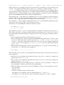
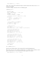
Download PH36010 Numerical Methods Worksheet 1 Using the PGPLOT

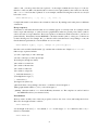
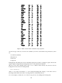
PH36010 Numerical Methods Worksheet 1
Using the PGPLOT libraries
The aim of this worksheet is learn how to incorporate external libraries into our Fortran 90 programs. The
particular library that we will consider is the PGPLOT library which adds two-dimensional graph plotting
capability to Fortran.
1. An example
Consider the following code
PROGRAM pgtest
IMPLICIT NONE
REAL, DIMENSION(21) :: xarr, yarr
INTEGER :: i, ier
INTEGER, EXTERNAL :: PGBEG
! Calculate values of COS(x) for 0<x<pi
DO i=1,21
xarr(i) = 6.28*REAL(i-1)/20.
yarr(i) = COS(xarr(i))
END DO
! plot a graph of y=COS(x)
ier=PGBEG(0,’?’,1,1)
IF (ier /= 1) STOP
CALL PGENV(0.0,7.0,-1.0,1.0,0,1)
CALL PGLINE(21,xarr,yarr)
CALL PGEND()
END PROGRAM pgtest
Type this code in (call it pgtest.f90) and compile and run it with the following commands
dob@fortran> f90 -o pgtest pgtest.f90 -lpgplot -lX11 -lpng
dob@fortran> ./pgtest
You will be prompted for a graphics device. Type /XWIN.
Run the code again, and instead of /XWIN, type ?, this will give you a list of possible graphics devices.
Of particular interest are /XWIN which we have already seen, /PNG which will produce a PNG graphics
file, and perhaps /PS which will produce postscript files.
For this example, enter /PNG. This should have created a file called pgplot.png. You can view this
by running
dob@fortran> xv pgplot.png &
Right clicking on the image will produce a user interface for manipulating the image.
Alternatively, we can transfer pgplot.png to our local machine using WinSCP, and use the local
graphics packages under Windows XP.
Explanation
This example has introduced several new concepts that we will now look at in more detail. First we will
look at the compilation line
1
dob@fortran> f90 -o pgtest pgtest.f90 -lpgplot -lX11 -lpng -L/usr/X11R6/lib
We have the basics of compiling code that we have previously seen, but there are a few new flags at the
end. The -l flag indicates the library that we wish to use, so in the above example, the flags -lpgplot
-lX11 -lpng indicate that we wish to use the pgplot library (which gives us our plotting routines)
along with the X11 library (which allows us to produce a new window and draw in it) and the PNG library
(which allows us to write png graphics files). Strictly speaking, our program only uses the PGPLOT
library, and the PGPLOT library then uses the X11 and PNG libraries.
The final flag is the -L flag. This tells us which directories to look in for libraries. Linux should know
where most libraries are stored, but a few libraries may be stored in unusual locations (for a variety of
reasons), so the -L flag directs the Fortran compiler to these extra locations.
The command xv is a Linux graphics package that allows us to view and manipulate graphics files (such
as pngs). We can use this to convert to other formats if we wish.
We will now look at the PGPLOT commands in a little more detail.
ier=PGBEG(0,’?’,1,1)
IF (ier /= 1) STOP
This initialises a new plot. PGBEG is an external function, and must be declared as such at the top of
the program. We output to an integer variable, which should return the value 1. If it does not, an error
has occured which we should deal with accordingly (in this case stop the program). The function takes 4
arguments:
• The first argument is historical, and should always be set to 0.
• The second argument is a character string that tells PGPLOT what graphics device to write to. This
can be any of the devices that you have seen above (e.g., ’/XWIN’, ’/PNG’, ’/PS’, etc). If
you put ’?’ then the program will ask which device you want. You may extend this further and
provide a name for your output file, so ’mypic.png/PNG’ will create a PNG with filename
mypic.png.
• The third and fourth arguments are used to place multiple plots on a page. For the time being, set
both of these to 1, so that we have just a single plot.
CALL PGENV(0.0,7.0,-1.0,1.0,0,1)
This subroutine sets up a new plot, providing information about the range, scale and setup of the plot. It
takes 6 arguments:
• The first two are real numbers that indicate the range of the x-axis, so in the above example, the
graph is plotted for 0.0 ≤ x ≤ 7.0.
• The second two are real numbers that indicate the range of the y-axis, so in the above example, the
graph is plotted for −1.0 ≤ y ≤ 1.0.
• The fifth argument gives the scaling of the plot, 1 scales the x- and y-axes equally (so 1 unit in x is
the same length as 1 unit in y), 0 scales the axes independently.
• The final argument controls the look of the surrounding box and axes. Some acceptable values are
-2
-1
0
1
2
No annotation
Draw box only
Draw box and label it with coordinate values
In addition to box and labels, draw axes with tick marks at x = 0 and y = 0
In addition to box, labels and axes, draw a grid at major increments of x- and y-coordinates
CALL PGLINE(21,xarr,yarr)
2
This subroutine plots a line on our graph, the arguments are the number of points that make up the line,
a 1D array of the x-points of the line and a 1D array of the y-points of the line.
CALL PGEND()
This subroutine ends our plot. All plots should be ended before the program ends, or moves on to do
another task (e.g., another plot).
2. Customising the plot
This plot is pretty bare, and often when we plot graphs we wish to customise them further, for example,
label the axes, plot data points and plot multiple lines.
Labelling the axes
Add the following line directly after the PGENV line
CALL PGLAB(’(x)’, ’(y)’, ’Graph of y=cos(x)’)
Compile and run this program. You will see that the two axes are labelled and the graph has a title. This
corresponds to the three arguments of the subroutine, they are all CHARACTER strings, the first is the
label for the x-axis, the second for the y-axis, and the third is the graph title.
If we wanted to leave one of these blank, we could pass an empty CHARACTER string.
Figure 1: Table of symbols available with the PGPT subroutine along with their reference numbers.
Plotting data points
Add the following line to the program after the PGLINE line
CALL PGPT(21,xarr,yarr,11)
3
Compile and run this program. You will see that a diamond has been placed at the location of each
point. The subroutine follows the same syntax as the PGLINE subroutine, except there is an additional
argument at the end. This is an integer which tells the subroutine what symbol you wish to use. A table
showing the more popular symbols can be seen in figure 1.
Plotting multiple lines
We may use the PGLINE and PGPT routines to plot as many lines on a graph as we wish. Modify your
existing program so that the plotting part looks like the following
! plot a graph of y=COS(x)
ier=PGBEG(0,’/XWIN’,1,1)
IF (ier /= 1) STOP
CALL PGENV(0.0,7.0,-1.0,1.0,0,1)
CALL PGLAB(’(x)’, ’(y)’, ’Graph of y=a*cos(x)’)
CALL PGLINE(21,xarr,yarr)
CALL PGPT(21,xarr,yarr,11)
CALL PGLINE(21,xarr,0.75*yarr)
CALL PGPT(21,xarr,0.75*yarr,11)
CALL PGLINE(21,xarr,0.5*yarr)
CALL PGPT(21,xarr,0.5*yarr,11)
CALL PGLINE(21,xarr,0.25*yarr)
CALL PGPT(21,xarr,0.25*yarr,11)
CALL PGLINE(21,xarr,-yarr)
CALL PGPT(21,xarr,-yarr,11)
CALL PGEND()
Compiling and running this shows that we have put multiple lines on the same plot. In this case we have
used variations on the same curve, but we could just as easily have completely different lines and points.
3. Line style, width and colour
When plotting lines (and in some cases points) we often want to change the lines style, thickness and
colour. This is particularly important if we have multiple lines on a plot, and wish to distinguish between
them.
PGPLOT offers a range of routines that will change the style, and any lines plotted after the change will
take that style.
Line style
The style of a line can be changed using the following routine
CALL PGSLS(n)
where the argument n is an integer between 1 and 5. This number will select from the following styles:
1
2
3
4
5
full line
long dashes
dash-dot-dash-dot
dotted
dash-dot-dot-dot
In your program, add a call to PGSLS before each PGLINE, changing the style (n) each time.
Line width
The default width of a line is as close to 0.13 mm as the device can manage. This is what we get when
we set the line width to 1. If we choose another number, then we will get multiples of this, so a line width
of 2 is double thickness, which is 0.26 mm, and so on. We can set the width of a line with the following
command:
4
CALL PGSLW(n)
where n is an integer indicating the width as discussed above. Like PGSLS, this must be called before
you plot the line.
In your program, set the thickness of each line to different values. Note how this also changes the plotted
diamonds. Try resetting the line width before plotting the diamonds.
Index
0
1
2
3
4
5
6
7
8
9
10
11
12
13
14
15
16+
Colour
Black (background)
White (default)
Red
Green
Blue
Cyan (Green + Blue)
Magenta (Red + Blue)
Yellow (Red + Green)
Red + Yellow (Orange)
Green + Yellow
Green + Cyan
Blue + Cyan
Blue + Magenta
Red + Magenta
Dark Gray
Light Gray
Undefined
R
0.00,
1.00,
1.00,
0.00,
0.00,
0.00,
1.00,
1.00,
1.00,
0.50,
0.00,
0.00,
0.50,
1.00,
0.33,
0.66,
G
0.00,
1.00,
0.00,
1.00,
0.00,
1.00,
0.00,
1.00,
0.50,
1.00,
1.00,
0.50,
0.00,
0.00,
0.33,
0.66,
B
0.00
1.00
0.00
0.00
1.00
1.00
1.00
0.00
0.00
0.00
0.50
1.00
1.00
0.50
0.33
0.66
Table 1: Table showing the default colour indices and the RGB proportions that make up the colour.
Colour
Colour is defined by a set of colour indices which usually range from 0-255. We can change our pen
colour at anytime in a plot, and anything draw after will use this colour (until we change is again). This
includes lines, points, text, and so on.
The pen colour is changed using the routine
CALL PGSCI(i)
where i is the number of the new index. Consider the final plotting block in your code, modify it as
follows
CALL
CALL
CALL
CALL
CALL
CALL
CALL
PGSCI(2)
PGSLS(5)
PGSLW(10)
PGLINE(21,xarr,-yarr)
PGSCI(7)
PGSLW(1)
PGPT(21,xarr,-yarr,11)
Compile and run your code. Try changing the colours of the other lines. Available colours can be seen in
table 1.
Defining your own colours
We can see in table 1 that there are 16 predefined colours, but the indices between 16-255 are undefined.
This gives us the option of defining our own colours. One method of defining colours on a computer
5
is to specify how much red, green and blue light are mixed to make the colour. The RGB ratios for the
predefined indices are shown in table 1. We can define our own colours by passing our own mixture ratios
to an index. This is done using the following routine:
CALL PGSCR(i, r, g, b)
where i is the index number that we wish to set, r, g, b are real numbers between 0 and 1 which indicate
the ratio of red, green and blue in our mixture. So for example,
CALL PGSCR(16, 1.0, 0.59, 0.0)
CALL PGSCI(16)
will define a index 16 as a bright orange and use it as the pen colour for the next lines/points plotted.
In your code, try defining and using your own colours.
Note, it is possible to redefine the default colours. Indeed, we must do this if we wish to change the
background/foreground colours. For example, if you write your plot to png format in order to include it
in a document, you may prefer to have a white background rather than a black one. To do this, add the
following two lines to you program before you call PGENV.
CALL PGSCR(0, 1.0, 1.0, 1.0)
CALL PGSCR(1, 0.0, 0.0, 0.0)
The first line redefines the background colour to white, the second redefines the default pen colour to
black.
Try this in your code.
4. Error bars
In physics, when we plot experimental data, we usually have an associated error which we would like to
indicate on our graph as error bars. We can do this with PGPLOT using one of the following routines
CALL PGERRY(n, x, ylo, yhi, t)
CALL PGERRX(n, xlo, xhi, y, t)
The first routine plots error bars in the y-direction (vertical), the second plots error bars in the x-direction
(horizontal). The calls are similar to PGPT or PGLINE in that the first number (n) is an integer giving
the number of points to be plotted for. x is a real array giving the x-positions of the error bars, ylo and
yhi give the lower-upper extent of the error bars in the y-direction. xlo, xhi, and y do a similar thing
for horizontal errors. The t argument is a real number giving the width of the terminals at the end of the
error bars.
So as an example, consider the following code
PROGRAM pgerrbars
IMPLICIT NONE
REAL, DIMENSION(11) :: xarr, yarr, err, ylo, yhi
INTEGER :: i, ier
INTEGER, EXTERNAL :: PGBEG
! Calculate some arbitrary data values
DO i=1,11
xarr(i) = REAL(i-1)/2.
yarr(i) = 6.5*EXP(-0.4*xarr(i))
6
err(i) = SQRT(yarr(i))/3.0
ylo(i) = yarr(i) - err(i)
yhi(i) = yarr(i) + err(i)
END DO
! Set up plot
ier=PGBEG(0, ’/XWIN’, 1, 1)
IF (ier /= 1) STOP
! Plot axes and label
CALL PGENV(0.0, 5.0, 0.0, 8.0, 0,1)
CALL PGLAB(’(x)’, ’(y)’, ’Data with Error Bars’)
! Plot data points and error bars
CALL PGPT(11, xarr, yarr, -4)
CALL PGERRY(11, xarr, ylo, yhi, 1.0)
! End plot
CALL PGEND()
END PROGRAM pgerrbars
Type this in, compile and run it. Try modify some of the settings as you see fit. Try adding in some
horizontal error bars as well.
Logarithmic plots
We have seen (e.g., in the Data Handling and Statistics laboratory) how it is often useful to plot graphs
with logarithmic axes. It is not possible to plot log-plots directly, however, there is a work around. We
may calculate the logarithm (to the base 10) of our data and plot that, but label the axes logarithmically.
To do this we change the final argument in PGENV. There are 3 new options
10 Draw box and label the x-axis logarithmically
20 Draw box and label the y-axis logarithmically
30 Draw box and label both axes logarithmically
We must also change the range of the log’d axes, so that it ranges over the log of the data. For example,
the following changes to our error bar program will display a plot where the y-axis has a logarithmic
scale.
! Plot axes and label
CALL PGENV(0.0, 5.0, LOG10(0.5), LOG10(8.0), 0, 20)
CALL PGLAB(’(x)’, ’(y)’, ’Data with Error Bars’)
! Plot data points and error bars
CALL PGPT(11,xarr,LOG10(yarr),-4)
CALL PGERRY(11, xarr, LOG10(ylo), LOG10(yhi), 1.0)
Add these changes to the error bar program, compile and run. Try changing the code so that the x-axis is
log’d instead/as well.
5. Annotating the graph
While in many situations we need no more text on a graph than the labelling on the axes, for more
complicated plots we often want to label features on the graph, this may include labelling different lines
or pointing out features with arrows.
For basic labelling we can use the following routine:
7
CALL PGTEXT(x, y, ’label’)
where x and y are the position (in the units of the plot) of the bottom-left corner of the text, and ’label’
is the text to be printed.
Consider for example, a cut down version of our initial program.
PROGRAM pgannot
IMPLICIT NONE
REAL, DIMENSION(21) :: xarr, yarr
INTEGER :: i, ier
INTEGER, EXTERNAL :: PGBEG
! Calculate values of COS(x) for 0<x<pi
DO i=1,21
xarr(i) = 6.28*REAL(i-1)/20.
yarr(i) = COS(xarr(i))
END DO
! plot a graph of y=a*COS(x)
ier=PGBEG(0,’/XWIN’,1,1)
IF (ier /= 1) STOP
! setup the plot
CALL PGENV(0.0,7.0,-1.0,1.0,0,1)
CALL PGLAB(’(x)’, ’(y)’, ’Graph of y=a*cos(x)’)
! plot the case where a=1
CALL PGLINE(21,xarr,yarr)
CALL PGPT(21,xarr,yarr,11)
CALL PGTEXT(6.3, 0.92, ’a=1.0’)
! plot the case where a=0.25
CALL PGLINE(21,xarr,0.25*yarr)
CALL PGPT(21,xarr,0.25*yarr,11)
CALL PGTEXT(6.3, 0.18, ’a=0.25’)
! plot the case where a=-0.5
CALL PGLINE(21,xarr,-0.5*yarr)
CALL PGPT(21,xarr,-0.5*yarr,11)
CALL PGTEXT(6.3, -0.47, ’a=-0.5’)
! end the plot
CALL PGEND()
END PROGRAM pgannot
Type this in and compile and run it. Try moving the labels around and changing the text.
This is fine for most cases, but sometimes we might want to do something a bit more intricate. A more
general command allows us to alter the justification and the angle the text is printed:
CALL PGPTXT(x, y, a, b, ’label’)
8
where x and y are the position the text is placed, a is the angle at which the text slopes, b is the justification of the text (0.0 is left justified, 0.5 is centred, 1.0 is right justified, other values are allowed),
and ’label’ is the text that is printed. So as an example, add the following line to the above code just
before the PGEND.
CALL PGPTXT(4.1, -0.5, 65.0, 0.5, ’a=1.0’)
Compile and run this code and note the orientation of the text. Try adding text in other places at different
orientations.
Escape sequences
Sometimes we will want characters that do not normally appear on our keyboards. For example, Greek
letters, super and subscripts, or symbols used as graph markers when we plotted points. These symbols
can be accessed as escape characters. These are sequences of characters which start with a \, but are not
printed directly. Instead they instruct PGPLOT to substitute another symbol, or they pass on directions
for the following text. For example, the \gx directive will convert the letter corresponding to x into the
Greek character equivalent. So if we modified our PGLAB call to
CALL PGLAB(’(\gh)’, ’(y)’, ’Graph of y=a*cos(\gh)’)
then the x-axis would be labelled with “(θ)” and the title would become “Graph of y = a ∗ cos θ”.
Other escape sequences include
\u start a superscript (or end a subscript)
\d start a subscript (or end a superscript)
\b backspace (though not delete)
\fn switch to normal font
\fr switch to Roman font
\fi switch to italic font
\fs switch to script font
\\ backslash character (\)
\x multiplication sign (×)
\. centred dot (·)
\A Angstrom symbol (Å)
\gx Greek letter corresponding to the letter x, a full list is shown in figure 2
\mnn graph marker number n (1-31), as shown in figure 1
\(nnnn) character number nnnn from the Hershey character set. The complete set can be found on
the PGPLOT website (see reference below)
Text attributes
We may wish to modify some of the text properties, such as size, font, colour, and background colour.
These are all straight forward to achieve.
CALL PGSCH(h)
sets the height of the text (h = 1.0 is default, h = 1.5 is 50% larger, h = 0.5 is half-size, and so on). h
must be a real number.
CALL PGSCF(f)
9
Figure 2: Table of Greek letters with their escape sequence.
sets the font type of the text, four fonts are available (as we have seen with the escape characters), these
are
1 normal font (default)
2 Roman font
3 italic font
4 script font
Changing this will change the font for all further displayed text (until you change it again), whereas the
escape sequence change will just change the font for a few characters in that line.
The text colour can be changed with a call to PGSCI which we have already seen, however, the text
background colour can also be changed with
CALL PGSTBG(i)
where i is one of the colour indices, or -1 for a transparent background. Setting i to the same colour as
the background will have the effect of erasing whatever is underneath the text.
So for an example, consider the PGTXT line in our previous code, adding the following lines
10
CALL
CALL
CALL
CALL
CALL
PGSCH(1.25)
PGSCF(2)
PGSCI(2)
PGSTBG(3)
PGPTXT(4.1, -0.5, 65.0, 0.5, ’a=1.0’)
will increase the text size by 25%, use the Roman font, and colour the text red on a green background.
Try changing the text using different escape sequences, and modify the text properties using the above
routines.
Further reading
PGPLOT has much more functionality than is described in this worksheet, for example, it can plot histograms,
contour plots and image data. The PGPLOT website which contains a much larger user manual and information
about downloading and installing PGPLOT can be found at:
http://www.astro.caltech.edu/∼tjp/pgplot/
11