1
R. Pitt
April 4, 2005
WinTR55 for Watershed Analyses
Example use of WinTR55 .........................................................................................................................................1
Program Description..............................................................................................................................................1
Example WinTR-55 Setup and Operation .............................................................................................................4
Example Applications to Construction Sites ...........................................................................................................12
Design Storms for Different Site Controls ..........................................................................................................15
The Use of WinTR-55 for Detention Pond Analyses ..............................................................................................16
Predevelopment Conditions.................................................................................................................................16
Post Development Conditions .............................................................................................................................25
Post Development with Pond...............................................................................................................................28
Summary..............................................................................................................................................................34
Important Internet Links ..........................................................................................................................................35
References ...............................................................................................................................................................35
Example use of WinTR55
The following discussion is summarized from the WinTR-55 user guide information, while the example uses the
previously described information.
A WinTR-55 work group was formed in the spring of 1998 to modernize and revise TR-55 and the computer
software. The current changes include: upgrading the source code to Visual Basic, changing the philosophy of data
input, developing a Windows interface and output post-processor, enhancing the hydrograph-generation capability
of the software and flood routing hydrographs through stream reaches and reservoirs.
The availability and technical capabilities of the personal computer have significantly changed the philosophy of
problem solving for the engineer. Computer availability eliminated the need for TR-55 manual methods, thus the
manual portions (graphs and tables) of the user document have been eliminated as official guidance. The WinTR-55
user manual (NRCS 2002a) covers the procedures used in and the operation of the WinTR-55 computer program.
Part 630 of the Natural Resources Conservation Service (NRCS) National Engineering Handbook provides detailed
information on NRCS hydrology and is the technical reference for WinTR-55.
Program Description
WinTR-55 is a single-event rainfall-runoff small watershed hydrologic model. The model generates hydrographs
from both urban and agricultural areas and at selected points along the stream system. Hydrographs are routed
downstream through channels and/or reservoirs. Multiple sub-areas can be modeled within the watershed.
Model Overview
A watershed is composed of subareas (land areas) and reaches (major flow paths in the watershed). Each subarea has
a hydrograph generated from the land area based on the land and climate characteristics provided. Reaches can be
designated as either channel reaches where hydrographs are routed based on physical reach characteristics, or as
storage reaches where hydrographs are routed through a reservoir based on temporary storage and outlet
characteristics. Hydrographs from sub-areas and reaches are combined as needed to accumulate flow as water moves
from the upland areas down through the watershed reach network. The accumulation of all runoff from the
watershed is represented at the watershed outlet. Up to ten sub-areas and ten reaches may be included in the
watershed.
1
WinTR-55 uses the TR-20 (NRCS 2002b) model for all of the hydrograph procedures: generation, channel routing,
storage routing, and hydrograph summation. Figure 10 is a diagram showing the WinTR-55 model, its relationship
to TR-20, and the files associated with the model.
TR-55 System
TR-55 Windows
Standard
Land use
Data
State
Rainfall Data
Custom
Dimen. Unit
Hydrograph
Land use
Pointer
File
Help
Text
Data
Displays
and Plots
TR-55
Input Data
TR-20
Input File
Name
Custom
Rainfall
Distribution
TR-20
Input Data
TR-20
Model
Debug
Error
Printed
Page
Legend
Data Flow
Program Flow
Hydrograph
Figure 10. WinTR-55 system schematic (NRCS 2002a).
Capabilities and Limitations
WinTR-55 hydrology has the capability to analyze watersheds that meet the criteria listed in Table 9:
Model Input
The various data used in the WinTR-55 procedures are user entered via a series of input windows in the model. A
description of each of the input windows follows the figure. Data entry is needed only on the windows that are
applicable to the watershed being evaluated.
Minimum Data Requirements. While WinTR-55 can be used for watersheds with up to ten sub-areas and up to ten
reaches, the simplest run involves only a single sub-area. Data required for a single sub-area run can be entered on
the TR-55 Main Window. These data include: Identification Data-User, -State, -County, -Project, and -Subtitle;
Dimensionless Unit Hydrograph; Storm Data; Rainfall Distribution; and Subarea Data. The subarea data can
be entered directly into the Subarea Entry and Summary table: Subarea name, subarea description, subarea flows
to reach/outlet, area, runoff curve number (CN), and time of concentration (Tc). Detailed information for the
subarea CN and Tc can be entered here or on other windows; if detailed information is entered elsewhere the
computational results are displayed in this window.
2
Watershed Subareas and Reaches. To properly route stream flow to the watershed outlet, the user must
understand how WinTR-55 relates watershed subareas and stream reaches. Figure 11 and Table 10 show a typical
watershed with multiple sub-areas and reaches.
Table 9. WinTR-55 Capabilities and Limitations (NRCS 2002a)
Variable
Minimum area
Limits
No absolute minimum is included in the software.
However, carefully examine results from sub-areas less
than 1 acre.
Maximum area
25 square miles (6,500 hectares)
Number of Subwatersheds
3-10
Time of concentration for any sub-area
0.1 hour < Tc < 10 hour
Number of reaches
0-10
Types of reaches
Channel or Structure
Reach Routing
Muskingum-Cunge
Structure Routing
Storage-Indication
Structure Types
Pipe or Weir
Structure Trial Sizes
3-3
Rainfall Depth1
Default or user-defined
0 – 50 inches (0-1,270 mm)
Rainfall Distributions
NRCS Type I, IA, II, III, NM60, NM65, NM70, NM75, or
user-defined
Rainfall Duration
24-hour
Dimensionless Unit Hydrograph
Standard peak rate factor 484, or user-defined (e.g.
Delmarva—see Example 3)
Antecedent Moisture Condition
2 (average)
1
Although no minimum rain depth is listed by the NRCS in the above table, it must be recognized that the original SCS curve
number methods, incorporated in this newer version, are not accurate for small storms. In most cases, larger storms used for
drainage design are reasonably well suited to this method. Pitt (1987) and Pitt, et al. (2002) showed that rain depths less than 2 or 3
inches can have significant errors when using the CN approach.
Figure 11. Sample Watershed Schematic (NRCS 2002a)
3
Table 10. Sample Watershed Flows (NRCS 2002a)
Subarea
Area I
Area II
Area III
Area IV
Area V
Area VI
Area VII
Area VIII
Area IX
Area X
Flows into
Upstream End of
Reach A
Reach C
Reach C
Reach B
Reach C
Reach E
OUTLET
OUTLET
Reach D
OUTLET
Reach
Flows into
Reach A
Reach B
Reach C
Reach D
Reach E
Reach C
Reach C
OUTLET
OUTLET
OUTLET
Reaches define flow paths through the watershed to its outlet. Each subarea and reach contributes flow to the
upstream end of a receiving reach or to the Outlet. Accumulated runoff from all sub-areas routed through the
watershed reach system, by definition, is flow at the watershed outlet.
Processes
WinTR-55 relies on the TR-20 model for all hydrograph processes. These include: hydrograph generation,
combining hydrographs, channel routing, and structure routing. The program now uses a Muskingum-Cunge method
of channel routing (Chow, et al. 1988; Maidment 1993; Ponce 1989). The storage-indication method (NRCS NEH
Part 630, Chapter 17) is used to route structure hydrographs.
Example WinTR-55 Setup and Operation
An application using WinTR-55 and an urban watershed example is shown on Figures 12 through 21. Figures 22
and 23 are other screens available in WinTR-55 that can be used to aid in the calculation of some of the site data,
while Figure 24 is used for detention facilities (structures).
Figure 12. WinTR-55 opening screen.
4
Figure 13. WinTR-55 small watershed basic information screen.
5
Figure 14. WinTR-55 reach data screen.
Figure 15. WinTR-55 reach flow path screen.
6
Figure 16. WinTR-55 reach routing screen.
Figure 17. WinTR-55 storm data screen (information automatically determined by location).
7
Figure 18. WinTR-55 event selection/run screen.
8
Figure 19. WinTR-55 calculated hydrograph summary screen.
9
Figure 20. WinTR-55 hydrograph plot screen.
Figure 21. WinTR-55 report generation screen.
10
Figure 22. WinTR-55 land use details screen (if data not directly entered).
Figure 23. WinTR-55 time of concentration details screen/calculator (if data not directly entered).
11
Figure 24. WinTR-55 structure data screen for detention facilities.
This WinTR-55 example resulted in a peak flow for the 2-yr storm of about 730 cfs, compared to the previously
calculated value of 910 cfs. This difference is due to the different routing procedure used, plus the more precise
hydrograph development procedure in the updated WinTR-55 version compared to the tabular hydrograph method.
Example Applications to Construction Sites
The following example outlines the hydrographic information needs and how they can be determined using WinTR55 for a small urban area, in case, a construction site. There are a number of situations where WinTR-55 (or TR-55)
can be used to advantage when evaluating construction sites, including the design of erosion and sediment controls.
These may include:
• Determination of flows going away from the site affecting downstream areas. Downstream erosion
controls may include filter fencing along the project perimeter, or sediment ponds, depending on flow conditions.
These controls must be completed before any on-site construction is started.
• Determination of upland flows coming towards the disturbed areas. These flows must be diverted by
swales or dikes, or safely carried through the construction sites. Channel design will be based on the expected flow
conditions. These controls must be completed after the downstream controls, and before any on-site controls are
started.
• Determination of on-site flows on slopes going towards filter fencing, sediment ponds, or other controls.
Needed to also evaluate shear stress on channels and on slopes.
Figure 25 is an example site regional map (drawn on a USGS quadrangle) showing a construction site, and
associated upland and downslope drainages. The previous discussion illustrated how it is possible to easily calculate
the runoff characteristics affecting the site and downslope areas for different rain conditions. In addition, detailed
site conditions for different project phases can also be evaluated for the design of appropriate erosion and sediment
controls.
12
Figure 25. Determination of general upslope and downslope drainage areas from hypothetical construction
site.
Figure 26 shows subdrainages for the upslope, downslope, and on-site areas for this example construction site. Table
11 summarizes the characteristics of these areas, along with the hydrologic information needs for each area. Most of
the site will be cleared and graded, except for the two small areas near the downslope edge. The upslope diversions
will carry the upslope water to the main channel. The runoff from the O1 and O2 on-site areas will be controlled by
slope mulches and filter fences, before the runoff drains to the on-site main channel. A sediment pond will be
constructed at the downslope property boundary before this main channel leaves the site.
13
Figure 26. Subdrainage areas on and near construction site.
14
Table 11. Upslope and On-Site Subdrainage Area Characteristics for Construction Site
Area
Notation
Location
Objective
Area
(acres)
Cover n
U1
Upslope – direct to on
site stream
Upslope – diversion to
on site stream
Hydrograph (to be
combined with U2 and U3)
Peak flow rate and
hydrograph (to be
combined with U1 and U3)
Peak flow rate and
hydrograph (to be
combined with U1 and U2)
Peak flow rate and
hydrograph
37.4
U2
U3
Upslope – diversion to
on site stream
O1
On site – drainage to
sediment pond and
main site stream (also
slope protection
needed)
On site – drainage to
filter fence and main
site stream (also
slope protection
needed)
On site – towards
perimeter filter fence
(also slope protection
needed)
On site – towards
perimeter filter fence
(also slope protection
needed)
On site – towards
perimeter filter fence
(also slope protection
needed)
On site – nothing (will
remain undisturbed)
On site – nothing (will
remain undisturbed)
O2
O3
O4
O5
O6
O7
0.4
Average
flow
path
slope
8%
CN
(all
“C”
soils)
73
Tc
(min)
29
14.6
0.4
11.5
73
25
2.4
0.4
12.7
73
20.7
12.6
0.011
10
91
3.5
Peak flow rate and
hydrograph
7.1
0.011
10.5
91
1.6
Peak flow rate and
hydrograph
6.1
0.011
5
91
4.1
Peak flow rate and
hydrograph
3.1
0.011
6.7
91
3.3
Peak flow rate and
hydrograph
1.8
0.011
11.3
91
1.5
na
1.3
0.24
6.7
na
na
na
0.3
0.24
10
na
na
Design Storms for Different Site Controls
All of the information needed to calculate the expected flows from these upslope and on-site areas is shown on
Table 12, except for the design storm. The area has a SCS type III rain distribution and the construction period will
be one year. The different site features will require different design storms due to the different levels of protection
that are appropriate. Table 12 lists the features and the (assumed) acceptable failure rates during this one year
period, along with the corresponding design storm frequency and associated 24 hr rain total appropriate for the area.
The design storms range from 4.0 to 8.4 inches in depth and the times of concentration range from 1.5 to 30 minutes.
The design rain intensities could be very large for some of these design elements.
Table 12. Example Acceptable Levels of Protection for Different Site Activities
Site Construction Control
Acceptable Failure Rate
during Site Construction
Activities
Design Storm
Return Period
(years)
Diversion channels
Main site channel
Site slopes
Site filter fences
Sediment pond
Downslope perimeter filter fences
25%
5%
10%
50%
5% and 1%
10%
6.5
20
10
1.9
20 and 100
10
15
24-hr Rain Depth
Associated with this
Design Storm Return
Period
5.5
6.6
6.0
4.0
6.6 and 8.4
6.0
The Use of WinTR-55 for Detention Pond Analyses
This example application of WinTR-55 demonstrates the use of this new program in evaluating detention ponds in a
watershed with multiple subdrainage areas. As noted in the User Guide, WinTR-55 has some limitations compared
to the more comprehensive TR-20 program. In the analysis of detention ponds (“structures”), the most important
limitation is the availability of only 3 types of outlet structures (a broad-crested weir, a 90o weir, and a pipe outlet).
The greatest concern is how the pipe outlet is considered (a short-tube approximation approach). The USDA
WinTR-55 team explained this as follows: This approximation uses the pipe diameter and the head on the pipe as the
total head (permanent pool elevation to outlet invert plus 1/2 diameter). This estimation of head, coupled with a
slightly different orifice flow coefficient (0.6 instead of 0.8), essentially cancel each other out and the result is a
higher discharge estimate for one type of pipe material versus a slightly lower discharge estimate for another. The
pipe materials checked were reinforced concrete and corrugated metal. Overall, the estimated differences were very
small. The future version of the User Manual will be rewritten to reflect this short tube flow assumption with a
disclaimer that if the user needs a more exact estimate they should use a different tool (SITES or a user-estimated
rating in TR-20). They also stated that Version 1.0 of WinTR-55 will keep the existing short-tube approximation for
pipe outlets of structures. A future version 2.0 of WinTR-55 will likely have the ability to enter a user-provided
stage-storage-discharge rating curve or more complete pipe rating curves.
WinTR-55 is a great improvement over the older TR-55 in that more accurate channel and reservoir routing is
provided. This Windows version of the program is also very easy to use and the provided graphical output options
enable efficient and rapid evaluations.
This simple example is comprised of two subwatersheds, a 500 undeveloped area and an adjacent 100 developing
area. Specific characteristics of these areas (soils, land use breakdowns, channel characteristics, etc.) are provided in
the following discussion. Initially, the pre-development conditions are examined, followed by developed conditions.
A preliminary design of a detention pond is then evaluated to attempt to provide similar discharge peak flows from
the developed watershed portion after development as before development.
Predevelopment Conditions
The following screen shows the basic site conditions. The screen also shows the location of the area (Tuscaloosa
County, Alabama), the selection of the standard dimensionless hydrograph, the selection of the area units, and
labels. The drop-down “options” menu was also used to select “English” units (actually US customary units). The
area, CN, and Tc values area entered and calculated in other screens and the information was automatically
transferred to this screen.
16
In order to enter the area, CN, and Tc screens, double-click on one of the cells in the columns under the desired
label. The following screen is opened when either the area or CN column is selected. The screen shows the complete
listing of available land uses and surface covers for each of the 4 hydrological soil groups (scrolling is needed to see
all the options). Type in the area associated with each condition for each area. In this example, the pre-development
condition is woods-grass combination in good condition, with B soils. Area 1 is 500 acres in size, while Area 2 (the
developing area) is 100 acres in size. These pre-development conditions are the same throughout the sub-areas, but it
is possible to select a variety of conditions and have the program automatically weight the overall CN. If desired, it
is possible to directly enter the CN value without using the calculator.
Although not noted in the WinTR-55 User Guide, the prior TR-55 guidance recommended that the range of CNs for
one area should be relatively narrow, with no more than an extreme difference of 5 in the CNs for any area. If the
CN values varied by more than 5, it was recommended that the sub-area be further divided to place the extreme
values in separate sub-areas. This was recommended to enable more accurate routing of sub-area flows compared to
using a composite CN based on a wide range of individual values.
17
18
The Tc calculation screen can be opened in the same way, by double-clicking on any cell under the Tc column. If
available, the Tc can be directly entered without using the calculator. The following screens show the examples for
sub-areas 1 and 2 (selected by using the drop-down option under “sub-area name”). The flow path described on the
screens needs to be pre-determined to be the critical Tc flow path (the path that requires the longest time for water
drainage, not the physically longest flow path necessarily).
As in TR-55, the Tc can be comprised of three components. The sheet flow length is now restricted to a maximum
length of 100 ft. Prior TR-55 guidance allowed a maximum length of 300 ft, but this was thought to be excessive by
the WinTR-55 development team. The “Surface (Manning’s n)” menu lists the available sheetflow roughness
values. These are substantially different than what would be appropriate for channel flow conditions for rougher
material. Smooth surfaces have similar values. The shallow concentrated flow surface drop-down options are
restricted to “paved” and “unpaved.” Two shallow concentrated flow segments are allowed. There are also two
channel segments allowed. These are usually designated as streams on USGS topographic maps.
The “Reach Data” also needs to be entered. These are not the channels described on the Tc screen. The Tc channels
are located within the sub-areas. The Reach channels are the channels into which the sub-areas discharge (and as
noted on the opening screen). This screen also asks for the receiving reach into which each reach discharges. It is
also possible to designate the outlet as the receiving reach, as in this example. This screen is also used to designate a
reach as a structure (“reaches” can be either channels or detention ponds, with the appropriate routing procedure
used). If the structure has already been described, then the structure name will appear on the structure name dropdown menu.
19
The “Reach Flow Path” should be selected to confirm that the model interpreted the entered the area and reach
connections correctly. This screen shows the basic watershed area conditions, plus shows the reaches each sub area
flows into, plus shows how the reaches are combined as they flow downstream. It is possible to construct and
evaluate a very complex set of sub-areas for evaluation. This example is about as simple as possible and still show
pond and sub area hydrographs can be combined.
Finally, the “Storm Data” must be selected, or entered. The following screen is available under the “GlobalData”
drop down main menu. If the “NRCS Storm Data” button is selected, the standard 24-hr rainfall amounts and
20
appropriate Rainfall Distribution Type are used, corresponding to the county selected on the first program screen. It
is possible to enter other rainfall amounts. WinTR-55 is an event model that is used for individual design storms,
although WinTR-55 can examine the entire set, or a sub-set, of the standard storms. Although the 24-hr rainfall
amounts are used, the critical rain intensity corresponding to the Tc is actually used to normalize the dimensionless
hydrograph.
The “Run” icon is then selected and the following screen appears. This screen is used to select which event(s) are to
be evaluated.
When the “Run” button is selected, after clicking on each desired rain, the program calculates the site runoff and
routes it through each reach. An embedded version of TR-20 is actually used to conduct the analyses, being much
better than the prior manual TR-55 procedures which required rather crude increments of important site factors. The
21
following screen is then automatically displayed after a run. This screen displays the TR-20 output screen, showing
the peak runoff conditions and times. It is also possible to select “WinTR-20 Reports” for more detailed output
information.
The “Output Definition”, or report writer, icon displays the following screen. This allows specific information to the
produced in a written report, or displayed on the computer screen.
22
The following is an on-screen report.
23
The following is the hydrograph that can be plotted by selecting the next to last icon on the top tool bar. The
selection screen allows different hydrographs to be displayed. This plot shows how the pre-development
hydrographs from the two sub-areas join for the complete hydrograph. The 10-year storm (having a 10% chance of
occurring in any one year) produces a peak flow of about 139 cfs in the developing watershed. The upland sub-area
peak flow was about 453 cfs, while these combined to create a total basin peak flow of about 522 cfs.
24
Post Development Conditions
The pre-development file was edited and re-saved (using the “save as” option under the file drop-down menu) to
reflect developed conditions in sub-area 2, as shown on the following screens:
25
The developed 100 acre sub-area is comprised of 25 acres of commercial, 25 acres of town houses, and 50 acres of
1/3 acre lot residential areas (notice that the individual CNs range from 72 to 92, much broader than a difference of
5. Therefore, this area should be further sub-divided to separate the individual land uses, if possible. They were not
in this example though).
26
The Tc factors also changed substantially for sub-area 2 after development:
When the same 10-year storm was evaluated, the following hydrograph was produced:
27
The upper sub-area (#1) had the same hydrograph characteristics, but the urbanized sub-area (#2) had a substantial
increase in runoff volume and peak flow rate. The above composite hydrographs also show that the peaks are much
more separated after development, with the hydrograph of the developed area to develop and recede much faster
than the slower responding upper area sub-area. The developed area now has a peak flow rate of 391 cfs, but
because the hydrograph components are more separated than for pre-developed conditions, the overall total peak
hydrograph actually decreases slightly, to about 518 cfs.
Post Development with Pond
Even though the total area peak flows are actually less after development with no pond, the site development
standards still required a detention pond to reduce the post-development peak flow to the pre-development levels for
the area undergoing development. The WinTR-55 suggests a simplified approach to size the needed pond based on
the difference in the runoff volumes for pre and post-development conditions, and restricting the pond outlet device
to the pre-development flow.
The “WinTR-20 Reports” lists the runoff depth, in watershed inches. The pre-development runoff was reported to be
1.95 inches (over 100 acres). This corresponds to about 16.2 acre-feet. The post-development runoff depth was
about 4.05 inches (also over the same 100 acres), corresponding to about 33.8 acre-feet. The difference (and
“required” pond storage) is therefore 17.6 acre-feet. The maximum pond discharge was the pre-development peak
flow (for the 10-year storm for this example) of 139 cfs.
The pond size can then be crudely sized using these values. However, this was to be a multi-purpose pond, also
providing water quality benefits. A rough guide for the pond surface area (the bottom of the storage layer) for water
quality benefits can be estimated to be about 3% of the watershed paved area, plus 0.5% of the watershed pervious
28
area. The CN menu presented the watershed % imperiousness areas for each development category. The commercial
area is assumed to have 85% impervious area, the high density residential area to have 65% imperviousness, and the
low density residential area to have 30% imperviousness. A simple calculation resulted in a pond bottom area (the
actual surface of the permanent pool, which needs to be at least 3 feet deep), of 1.78 acres. A value of 2 acres will
therefore be used. If this portion of the pond is 6.5 feet deep, and the top area is 3.5 acres, the pond side slopes
would be about 7.3:1 (H:V), a reasonable value, to provide about 17.6 acre-feet of storage.
The first step was to describe the pond and to edit the post-development file to change Reach B from a channel to a
pond. The following is the description of the pond “structure” using the “Structure Data” top menu bar option. The
pond surface areas are described using the above calculated estimates. The area is 2 acres at the depth where the
discharge begins, and is 3.5 acres in area 6.5 feet above this spillway elevation. WinTR-55 will assume a deeper
pond as needed (above 6.5 feet) but will use this side slope. If the upper area was not entered (it is an optional
value), the pond is assumed to then have vertical side slopes (not a good idea). The Discharge Description” is based
on the spillway type selected, either a pipe (using the pipe approach previously described), or a weir. If a weir is
selected, it can be a broad-crested weir and the weir length entered. If a 0 value is entered for the weir length, the
model will assume a 90o V-notch weir. If a pipe spillway is selected (as in this example), the pipe diameter (in
inches) is given, ranging from 6 to 60 inches. When a pipe is selected, the height from the invert of the discharge
end of the pipe to the spillway elevation is also needed for the simplified equation. This height must be at least twice
the diameter of the pipe. Up to three pipe diameters (or weir lengths) can be entered. The model will evaluate all
three options, making the selection of the choice easier. As the dimensions are entered, the rating curves (flow vs.
height) and storage below the elevations are displayed. This is a good indication of the correct spillway size, as the
maximum discharge close to the desired pond depth can be observed. In this case, the 40 inch pipe has the desired
discharge of 139 cfs at a stage slightly above 4 feet, and well under 10 feet. The 36 inch pipe option would need
about 10 feet of stage (greater than planned), while the 24 inch pipe would require even more (more than 20 ft).
Therefore, it is expected that the 3rd pipe option, the 40 inch pipe would work best.
29
A rating curve can also be plotted for each outlet option if the “Plot” option is selected on the structure screen. This
plot confirms that the 40 inch pipe discharge would require about 5 feet of the available pond stage.
30
The reach is then modified to be a pond instead of a creek. The “Structure Name” drop-down menu in the
appropriate cell is used to select the available pond name (available after the “accept” button on the pond menu is
clicked). The creek data, if previously on the reach data menu row for the named reach that is now a pond, needs to
be deleted.
31
The “Reach Flow Path” screen (selected from the “Project Data” drop down menu) can also be selected to ensure
that the model has the outfall, reaches and areas correctly connected:
32
Upon program execution, the data can be reviewed to verify if any of the spillway options were suitable. The
following table shows that trial #3 (the 40 inch pipe) reduces the reach B influent flow (391 cfs) down to about 130
cfs, close enough to the desired maximum peak flow. Unfortunately, the outfall peak flow is shown to be about 580
cfs, substantially greater than the predevelopment peak flow of 521 cfs and the post development peak flow, with no
pond, of 518 cfs.
The following plot of the reach hydrographs indicate how this occurred. The water from subarea 2 was delayed in
the detention pond (Reach B) and was discharged so that its peak rate closely coincided in time with the
undeveloped hydrograph from subarea 1 (Reach A), causing a larger peak flow than if the water was not detained.
33
This example illustrated how a detention pond can be evaluated for a developing area, how it can be designed for
multiple objectives, and how these objectives may, or may not, be realized in a watershed. The simple application of
detention pond standards may not always provide the desired downstream benefits. A basin-wide hydrologic
analysis (the above example was a crude and simple example) is needed to ensure that ponds area sized and located
correctly to provide the desired benefits. Obviously, the above example was a set-up to illustrate this issue.
However, it would be relatively easy to modify the pond to still provide the desired water quality benefits, while not
exasperating the flood control objective. A change in the pond spillway device to allow the pond to empty more
rapidly would solve this problem. In most cases, detention ponds providing large amounts of storage for flood
control should be located in upper reaches of watersheds to lessen these problems.
Summary
WinTR-55 is probably the simplest (and cheapest!) model that can be used to examine basin-wide hydraulic issues.
It is relatively simple to use and is based on conventional drainage design procedures. Future improvements in the
spillway options will make it more accurate. If more precise analyses are needed, TR-20, or more sophisticated
models should be used. It must also be emphasized that WinTR-55 (and TR-20) are not suitable models for water
quality evaluations. The curve number approach is not applicable for the moderate-sized events that are responsible
for the vast majority of pollutant discharges, continuous simulations for long periods are needed to understand the
complex behavior of pollutant discharges under a wide range of environmental conditions, and particle routing
34
(including scour from shallow and dry ponds) is needed to predict the level of pollutant control that may be achieved
in detention ponds. However, multiple tools can be used together to better understand how multiple (and often times,
conflicting) objectives can be met.
Important Internet Links
Alabama Rainfall Atlas:
http://bama.ua.edu/~rain/
WinTR-55 computer program (windows beta version):
http://www.wcc.nrcs.usda.gov/hydro/hydro-tools-models-wintr55.html
TR-55 1986 documentation:
ftp://ftp.wcc.nrcs.usda.gov/downloads/hydrology_hydraulics/tr55/tr55.pdf
TR-20 computer program (new windows beta version):
http://www.wcc.nrcs.usda.gov/hydro/hydro-tools-models-wintr20.html
National Engineering Handbook, Part 630 HYDROLOGY
http://www.wcc.nrcs.usda.gov/hydro/hydro-techref-neh-630.html
US Army Corps of Engineers, Hydrologic Management System User Guide (HEC HMS) (replacement for HEC-1):
http://www.hec.usace.army.mil/software/hec-hms/hechms-hechms.html
US Army Corps of Engineers, River Analysis System User Guide for water surface profile calculations (HEC RAS)
(replacement for HEC-2):
http://www.hec.usace.army.mil/software/hec-ras/hecras-hecras.html
References
Chow, V. T., Maidment, D. R, and Mays, L. W., Applied Hydrology, McGraw-Hill, 586 pages. 1988.
HEC. HEC-RAS User's Manual, Version 2.0. US Army Corps of Engineers, Hydrologic Engineering Center, April
1997.
Illinois. Illinois Procedures and Standards for Urban Soil Erosion and Sedimentation Control. Association of
Illinois Soil and Water Conservation Districts, Springfield, IL 62703. 1989.
Maidment, D. R. (ed.), Handbook of Hydrology, McGraw-Hill, 1422 pages. 1993.
McGee, T.J. Water Supply and Sewerage. McGraw-Hill, Inc., New York. 1991.
NRCS. National Engineering Handbook, Part 630 HYDROLOGY, downloaded June 23, 2002 at:
http://www.wcc.nrcs.usda.gov/water/quality/common/neh630/4content.html
NRCS. SITES Water Resource Site Analysis Computer Program User’s Guide. United States Department of
Agriculture, Natural Resources Conservation Service. 469 pp. 2001.
NRCS. WinTR-55 User Manual. US Dept. of Agriculture, Natural Resources Conservation Service. Downloaded on
June 23, 2002 from: http://www.wcc.nrcs.usda.gov/water/quality/common/tr55/tr55-beta.html Version dated April
23, 2002a.
NRCS. TR-20 System: User Documentation. United States Department of Agriculture, Natural Resources
Conservation Service. 105 pp. 2002b (draft).
Pitt, R. Small Storm Urban Flow and Particulate Washoff Contributions to Outfall Discharges, Ph.D. Dissertation,
Civil and Environmental Engineering Department, University of Wisconsin, Madison, WI, November 1987.
35
Pitt, R. and S.R. Durrans. Drainage of Water from Pavement Structures. Alabama Dept. of Transportation. 253 pgs.
September 1995.
Pitt, R., J. Lantrip, R. Harrison, C. Henry, and D. Hue. Infiltration through Disturbed Urban Soils and CompostAmended Soil Effects on Runoff Quality and Quantity. U.S. Environmental Protection Agency, Water Supply
and Water Resources Division, National Risk Management Research Laboratory. EPA 600/R-00/016.
Cincinnati, Ohio. 231 pgs. December 1999.
Pitt, R., M. Lilburn, S. Nix, S.R. Durrans, S. Burian, J. Voorhees, and J. Martinson Guidance Manual for Integrated
Wet Weather Flow (WWF) Collection and Treatment Systems for Newly Urbanized Areas (New WWF Systems).
U.S. Environmental Protection Agency. 612 pgs. Expected final publication in 2002.Ponce, V.M., Engineering
Hydrology, Prentice Hall, 640 pages. 1989.
SCS. Urban Hydrology for Small Watersheds. Technical Release 55, US Department of Agriculture, Soil
Conservation Service. 91 pp. 1975.
SCS (now NRCS). Urban Hydrology for Small Watersheds. US Dept. of Agric., Soil Conservation Service. 156 pgs.
1986.
SCS. Time of Concentration, Hydrology Technical Note No. N4. United States Department of Agriculture, Soil
Conservation Service, Northeast National Technical Center. 12 pp. 1986.
Thronson, R.E. Comparative Costs of Erosion and Sediment Control, Construction Activities. U.S. Environmental
Protection Agency. EPA430/9-73-016. Washington, D.C. 1973.
Welle, P.I., Woodward, D. E., Fox Moody, H., A Dimensionless Unit Hydrograph for the Delmarva Peninsula,
Paper No. 80-2013, ASAE 1980 Summer Meeting, 18 pp. 1980.
36