Download User manual v.2.0

© 2004-2008 Atte Moilanen
Zonation
Software for spatial conservation prioritization
by Atte Moilanen
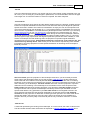
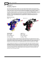
Zonation is a spatial conservation prioritization framework
for large-scale conservation planning. It identifies areas,
or landscapes, important for retaining high habitat quality
and connectivity for multiple biodiversity features (eg.
species), providing a quantitative method for enhancing
species' long term persistence.
Essentially, this software is a decision support tool for all
non-commercial parties working on conservation issues.
As Zonation operates on large grids, it provides a direct
link between GIS, statistical distribution modeling and
spatial conservation prioritization.
The Zonation framework is presently under constant
development and the next version of the software can be
expected not too far in the future. Thus, keep an eye on
our web site:
www.helsinki.fi/bioscience/ConsPlan
Zonation - User manual
© 2004-2008 Atte Moilanen
All rights reserved. USE THIS SOFTWARE AT YOUR OWN RISK. THE AUTHOR WILL NOT BE LIABLE FOR ANY
DIRECT OR INDIRECT DAMAGE OR LOSS CAUSED BY THE USE OR THE INABILITY TO USE THIS SOFTWARE.
CONDITIONS OF USE: Zonation v. 2.0 is freely usable for non-commercial uses. For any other kinds of uses, contact
the author for permission.
Do not use this software if you disagree with the disclaimer and conditions of use.
Even though the ZIG software has been done with the best of intentions, it is quite beyond one researcher to ensure
its correct operation under all operating systems and environments. Also anticipating and checking for all
combinations of erroneous input has not been possible. Therefore, use the software with care and make an effort to
understand the output and make a reality check as to whether the results make logical sense.
Publisher
Atte Moilanen/ Metapopulation
Research Group
Managing Editor
Atte Moilanen
Technical Editors
Heini Kujala
Anni Arponen
Cover Designer
Heini Kujala
Atte Moilanen
Cover Photo
Heini Kujala
Evgeniy Meyke
Special thanks to:
Anni Arponen, Alison Cameron, Aldina Franco, Ascelin Gordon,
John Leathwick, Grzegorz Mikusinski, Chris Thomas and Brendan
Wintle are thanked for comments on the software and its functions
and usability.
Special thanks to Anni Arponen who helped with an early version of
Zonation documentation, and to Mar Cabeza, who commented the
first version of the manual. Brendan Wintle generously provided
sample data files from the Hunter Valley region to be included in
the tutorial, and Evgenyi Meyke kindly provided beautiful
background photographs for the Zonation documentation.
Thanks to all who have collaborated in the development of
Zonation methods and applications.
This work has been supported by the Academy of Finland project
1206883 to the author, and two Academy of Finland Centre of
Excellence grants (2000-2005 and 2006-2011) to the MRG lead by
Academy professor Ilkka Hanski.
Helsinki, February 26, 2008
Atte Moilanen
Academy Research Fellow
Metapopulation Research Group
Dept. Biological and Environmental Sciences
P.O. Box 65
FI-00014 University of Helsinki
Finland
I
Zonation - User manual
Table of Contents
2
Part I Introduction
1 Aim & purpose
........................................................................................................................... 2
........................................................................................................................... 3
2 The Zonation framework
...........................................................................................................................
4
3 Zonation compared
to other reserve selection approaches
Zonation .............................................................................................................................................................
.............................................................................................................................................................
Integer programming
4
4
Stochastic.............................................................................................................................................................
global search
5
6
4 A typical Zonation...........................................................................................................................
work flow
...........................................................................................................................
8
and quick start
5 Software installation
6 New features
........................................................................................................................... 11
15
Part II Methods & algorithms
1 References
........................................................................................................................... 15
........................................................................................................................... 16
2 The Zonation meta-algorithm
17
3 The cell removal...........................................................................................................................
rule
.............................................................................................................................................................
Basic core-area
Zonation
.............................................................................................................................................................
Additive benefit function
17
18
.............................................................................................................................................................
Target-based
planning
.............................................................................................................................................................
General differences
between cell removal rules
20
.............................................................................................................................................................
Generalized
benefit function
22
20
24
4 Inducing reserve...........................................................................................................................
network aggregation
.............................................................................................................................................................
Distribution
smoothing
Boundary.............................................................................................................................................................
Quality Penalty (BQP)
Boundary.............................................................................................................................................................
Length Penalty (BLP)
.............................................................................................................................................................
Directed connectivity
(NQP)
25
25
28
28
........................................................................................................................... 31
5 Uncertainty analysis
.............................................................................................................................................................
Uncertainty
in species distributions, distribution discounting
.............................................................................................................................................................
Uncertainty
in the effects of landscape fragmentation
31
35
...........................................................................................................................
37
analysis
6 Replacement cost
........................................................................................................................... 39
7 Species interactions
........................................................................................................................... 42
8 Assumptions & limitations
44
Part III ZIG - The Zonation software
1 Introduction
........................................................................................................................... 44
........................................................................................................................... 44
2 Running Zonation
Command.............................................................................................................................................................
prompt
Windows.............................................................................................................................................................
interface
Batch-run.............................................................................................................................................................
capability
.............................................................................................................................................................
Loading previously
calculated Zonation solutions
44
45
46
48
........................................................................................................................... 49
3 Input files & settings
.............................................................................................................................................................
Introduction
.............................................................................................................................................................
Compulsory files
49
49
Species distribution
....................................................................................................................................................
map files
49
Species list
....................................................................................................................................................
file
50
© 2004-2008 Atte Moilanen
Contents
II
Run settings
file
....................................................................................................................................................
.............................................................................................................................................................
Optional files
53
58
SSI list and
....................................................................................................................................................
coordinates
58
Planning unit
....................................................................................................................................................
layer
59
Cost layer....................................................................................................................................................
60
Removal ....................................................................................................................................................
mask layer
61
Distributional
....................................................................................................................................................
uncertainty map layer
62
Uncertainty
....................................................................................................................................................
analysis weights file
63
Boundary....................................................................................................................................................
quality penalty definitions file
63
Directed connectivity
....................................................................................................................................................
description file
64
Species interactions
....................................................................................................................................................
definition file
65
...........................................................................................................................
67
4 Standard Zonation
output
.............................................................................................................................................................
Visual output
.............................................................................................................................................................
Automated
file output
67
73
5 Main analyses ........................................................................................................................... 77
.............................................................................................................................................................
Basic Zonation
and species weighting
.............................................................................................................................................................
Distribution
smoothing + Zonation
77
79
.............................................................................................................................................................
BQP Zonation
.............................................................................................................................................................
Directed connectivity
81
Including.............................................................................................................................................................
distributional uncertainty - Distribution discounting
.............................................................................................................................................................
Species interactions
86
.............................................................................................................................................................
Inclusion/Exclusion
cost analyses using mask files
91
83
89
95
analyses & options
6 Post-processing...........................................................................................................................
.............................................................................................................................................................
Landscape
identification
Statistics.............................................................................................................................................................
for management landscapes
95
97
............................................................................................................................................................. 99
Solution comparison
.............................................................................................................................................................
100
Fragmentation
uncertainty anlysis
Solution.............................................................................................................................................................
cross-comparison using solution loading
.............................................................................................................................................................
ZIG_Sum
Utility
102
.............................................................................................................................................................
Obtaining
species-specific information about solution quality
105
103
107
7 Data limitations...........................................................................................................................
& system requirements
........................................................................................................................... 108
8 Troubleshooting
...........................................................................................................................
110
9 Tips for using the
command prompt
Part IV Tutorial & Examples
113
1 Exercise 1
........................................................................................................................... 115
2 Exercise 2
........................................................................................................................... 117
3 Exercise 3
........................................................................................................................... 118
4 Exercise 4
........................................................................................................................... 120
5 Exercise 5
........................................................................................................................... 122
6 Exercise 6
........................................................................................................................... 123
7 Exercise 7
........................................................................................................................... 124
8 Exercise 8
........................................................................................................................... 126
Index
© 2004-2008 Atte Moilanen
128
Part
I
Introduction
1
Introduction
1.1
Aim & purpose
2
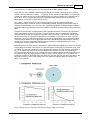
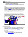
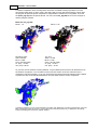
Zonation is a reserve selection framework for large-scale spatial conservation planning. It
identifies areas, or landscapes, that are important for retaining habitat quality and connectivity for
multiple species, thus providing a quantitative method for enhancing species' long term
persistence.
Zonation produces a hierarchical prioritization of the landscape based on the biological value of
sites (cells), accounting for complementarity. The algorithm proceeds by removing least valuable
cells from the landscape while minimizing marginal loss of conservation value, accounting for
connectivity needs and priorities given for biodiversity features (species, landcover types etc.). As a
result, a nested sequence of highly connected landscape structures is obtained with the core areas
of species distributions remaining latest and previously-removed areas showing as buffer zones. In
this way, landscapes can be zoned according to their potential for conservation, and differing
degrees of protection, maintenance or restoration effort can be applied to different zones. The
purpose is not necessarily to produce a detailed conservation plan for a large region, but to identify
priority areas of the landscape that could be subjected for more detailed analysis and planning that
accounts for other land-use pressures than nature conservation.
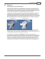
The Zonation software has been geared towards using large grids as input data, facilitating a direct
link between GIS, statistical distribution modeling and Zonation. It is particularly simple to input
modeled species distributions (or land cover types) into Zonation. First do statistical habitat models
for species, then predict species occurrence across the landscape grid, then feed the grids into
Zonation. The Zonation software can be run with relatively large datasets on an ordinary desktop
PC.
The Zonation software is intended for the analysis of biological data with the aim of finding out
spatially good conservation solutions. In this process Zonation purposefully ignores other land use
planning considerations, such as commercial or recreational values (except for what can be
entered as simple cost/mask layers). Thus, output of Zonation should be seen as an analysis of
conservation value which feeds into a broader land use planning framework where political
decisions are made that balance between different land use needs.Note that Zonation can also be
used for identifying the least important parts of the landscape, those in which human activity would
cause least harm to biodiversity value.
© 2004-2008 Atte Moilanen
3
1.2
Zonation - User manual
The Zonation framework
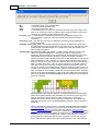
Aim and purpose
To provide a tool for large-scale high-resolution spatial conservation planning using primarily
GIS grid data
Analyses
Identification of optimal reserve areas
Identification of least useful conservation areas
Replacement cost analysis for current or proposed reserves
Planning methods
- Core-area Zonation
- Additive benefit function
- Target-based benefit function
Data
Large-scale grids with
- Presence/absence -data
- Probabilities of occurrence
- Abundance/density -data
- Cost and mask layers
Point observation data (New in v. 2.0)
Planning unit layers (New in v. 2.0)
Features
Methods for dealing with connectivity needs of species
- Distribution Smoothing (species-specific)
- Boundary Quality Penalty (species-specific)
- Boundary Length Penalty
- Directed Freshwater Connectivity (species-specific) (New in v. 2.0)
Uncertainty analysis aiming at reliable conservation decisions
Species weighting
Clearly defined trade-offs between species
Species interactions (New in v. 2.0)
© 2004-2008 Atte Moilanen
Introduction
1.3
4
Zonation compared to other reserve selection approaches
In this section we comment on the differences between Zonation and other commonly used
approaches to reserve selection. This comparison is not meant to be exhaustive nor completely
referenced, but rather, to give an indication of the most fundamental differences (that we believe to
exist) between these methods. This section will also be outdated when new features are developed
into other conservation planning softwares.
1.3.1
Zonation
Input data. Zonation is targeted for use with large grid-based data sets. This implies that species
distributions, used within Zonation, might be produced using some predictive statistical technique
using environmental layers as predictors for species presence/abundance. Data sets in the order of
millions of grid cells can be analyzed.
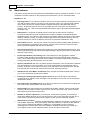
Output. Instead of outputting the optimal set of sites for achieving targets, Zonation outputs (1) the
hierarchy of cell removal throughout the landscape and (2) species loss curves. This kind of output
has multiple advantages.
(i) The result for a range of targets is immediately obvious,
(ii) there is an indication of the importance of all cells, both inside and outside any given
fraction,
(iii) the curves show how well (relatively) individual species do at any given fraction of the
landscape, and
(iv) the curves indicate the relative value of the solution as well as the stability of the solution.
(v) the zonation output lends itself to easy visualization
We will elaborate the item (iv). If species performances are declining rapidly at the chosen
landscape fraction, it means that the solution is not stable with respect to uncertainty in input data,
and that smallish changes in the selected fraction and / or spatial pattern might have large
consequences for species. If the species performances are stable at the chosen fraction, then
small changes in the fraction/spatial pattern are unlikely to have any significant effect on the
solution quality.
Additionally, the core-area Zonation method has a specific feature in that it emphasizes best areas
for all species, instead of treating low-to-medium quality locations as additive.
Optimality. The optimality characteristics of Zonation have not been conclusively examined, but
this is our present evaluation of this issue.
(i) Zonation using additive benefit functions or the targeting benefit function (above the target) is
very close to globally optimal. This is because with these cell removal rules the optimization
problem is convex and can thus be solved using a gradient-like iterative heuristic. (van Teefelen
and Moilanen 2008). Also, with the additive cell removal rules the degree of suboptimality goes
down when the landscape size (number of cells) increases. Thus optimality is not a problem with
the additive cell removal rules. Except, use of the Boundary Quality Penalty BQP renders the
problem non-convex (especially if some species benefit from fragmentation), and the degree of
sub-optimality of the solution is unknown.
(ii) The core-area Zonation. This method has so far only been defined algorithmically, not in an
objective function form (the CAZ cell removal rule specifies a difference equation for conservation
value but not the objective directly), and the degree of suboptimality of results is unknown. Then
again, no other implementation of this method is available.
1.3.2
Integer programming
Input data. Can accept arbitrary sites as well as grid cells. According to a relatively recent review,
Williams et al. (2004), the data size limits of IP were at that time around 10000 landscape
elements, which as a grid is only 100x100 elements. This is orders of magnitude less than the data
limits of Zonation, which can run landscapes of 10+ millions of elements even when using the
© 2004-2008 Atte Moilanen
5
Zonation - User manual
Boundary Quality Penalty.
Output. Globally optimal set of sites achieving targets. No prioritization through the landscape, no
performance curves.
Optimality. Guaranteed globally optimal solution to a simplified problem. The value of the global
optimality of results is compromised by the requirement that both the objective function and
constraints need to be linear (or that they can be linearized). In a sense you have the optimal
solution to the wrong (simplified) problem. Not applicable, at least not easily, to species-specific
connectivity calculations on large landscapes.
Williams, J., C.S. ReVelle, and S.A. Levin. 2004. Using mathematical optimization models to
design nature reserves. Frontiers in Ecology and the Environment 2: 98–105.
1.3.3
Stochastic global search
Stochastic global search includes techniques such as simulated annealing (SA; as in MARXAN)
and genetic algorithms (GAs).
Input data. In principle can be run on extremely large problems with few constraints on the
complexity of the problem. SA can handle larger problems than a GA, because of the memory
requirement for storing the GA population.
Output. A solution to the problem, typically of unknown quality. In some cases it may be possible to
devise an analytical method that provides bounds on solution quality (as in Moilanen 2005), which
then changes the method from a heuristic to an approximation. (Heuristic = method for which the
quality of results is unknown; approximation = method for which the maximum degree of
suboptimality of the results has been quantified in a non-trivial manner.)
Optimality. Degree of suboptimality will be highly dependent on (1) the size of the data, (2) the
complexity of the problem, like does it have nonlinear connectivity components in it, and (3) the
details of the implementation of the optimization algorithm. SA and GA are no way standard
algorithms (except for the high-level meta-algorithm). They can be varied in endless ways, in
particular, in terms of how they generate the new solutions to evaluate. If search starts far from the
good regions of the search space, it actually is not guaranteed that the good regions are found at
all. Good convergence with large problems absolutely is not guaranteed. Multiple runs from
different starting points are required to test for indications of convergence – and if multiple runs
reliably converge to a very similar result, then this indeed is an indication that the solution probably
is quite acceptable in terms of optimality. Probably are ok with smallish data sets with thousands or
tens of thousands of sites, but at the million-element scale the performance of these methods is
poorly known. Relative performance probably degrades when problem size increases, which is
opposite from what is actually expected for Zonation, at least with the additive cell removal rules.
There are piles of literature on optimization, which is an enormous field of science in itself. See the
references below for examples of the use of stochastic optimization on nonlinear reserve selection
problems. Also check MARXAN reserve selection software user manual and references therein.
Moilanen, A. 2005. Reserve selection using nonlinear species distribution models. American
Naturalist 165: 695-706. AND in particular its electronic appendixes A-C.
Moilanen, A. and M. Cabeza. 2002. Single-species dynamic site selection. Ecological Applications
12: 913-926.
For a more philosophical intro to these optimization methods see
Moilanen, A. 2001. Simulated evolutionary optimization and local search: Introduction and
application to tree search. Cladistics 17: 512-525.
© 2004-2008 Atte Moilanen
Introduction
1.4
6
A typical Zonation work flow
This section outlines a typical sequence of steps that would be done for the Zonation analysis of
one data set.
(i) Get the basic analyses running
i.1. Install Zonation, and get the basic zonation running with the example files provided.
i.2. Decide your cell removal rule.
i.3. Produce a new settings file, species list file etc. for your own data and check that you are
able to run the basic analysis (without aggregation methods or uncertainty analysis).
i.4. Try variants of the basic analysis by adding unequal species weights, aggregation methods
and uncertainty analysis. You can use solution comparison to check how big a difference
does the addition of one complication cause into the solution. These preliminary analyses
can as well be run using high warp-factors (100-1000) to reduce runtimes.
(ii) Identify your base-analysis. There are endless options of what species weights to give, what
species-specific parameters exactly to use in the aggregation method (distribution discounting or
boundary quality penalty) and what parameter(s) to use in the uncertainty analysis. You cannot run
all combinations of everything and indeed it is not useful to do so. Therefore, after getting the basic
Zonation running, you need to decide the most reasonable options for your analysis. These options
would depend on the availability of data and on your planning needs. Things that need to be
decided include
ii.1 Decide species weights. Equal weights is the basic option but there may well be good
reason to favour particular species by giving them more weight.
ii.2 Decide about how to induce aggregation into the final solution. Options include distribution
smoothing, boundary quality penalty, directed freshwater connectivity and boundary length
penalty. In general, you want aggregation at least if your planning units are small, like
hectares or so, because with small selection units population dynamics of nearby cells are
strongly linked. If planning units are very large, like 10x10km cells, then aggregation could
plausibly be omitted.
ii.3 Decide if some amount of distribution discounting uncertainty analysis would be
appropriate.
(iii) Base-analysis and sensitivity analysis. At this point you have identified the analysis options
which you believe to be most appropriate. Next
iii.1 Run your base-analysis, preferably using a relatively low warp factor.
iii.2 Run variants around your base-analysis varying a single analysis feature at a time (you
probably cannot run all combinations of everything). This is essentially a sensitivity
analysis, which is done by varying weights, aggregation and uncertainty analysis settings
within reasonable bounds. Investigate using solution comparison how big a difference
various options make.
iii.3 An analysis of selection frequency (with ZIG_Sum utility) may provide useful summary
information over analyses.
At this point you have a good idea of how different planning options influence your analysis and
solutions.
(iv) Identification of reserve areas. Identify management landscapes and check their statistics to
find out why different areas are important – what are the biodiversity features that occur there?
© 2004-2008 Atte Moilanen
7
Zonation - User manual
(v) Evaluation of proposed reserve areas using replacement cost analysis. If you need to
evaluate proposed or existing reserve areas, you can do that using mask files and replacement
cost analysis. This involves repeating your base analysis both with and without existing/proposed
areas included/excluded.
© 2004-2008 Atte Moilanen
Introduction
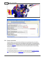
1.5
8
Software installation and quick start
Installation
The installation package includes the Zonation program (zig2.exe), the ZIG_Sum utility
(zig_sum.exe), a user manual (pdf) and tutorial files. You can find the installation package via the
Metapopulation Research Group website:
www.helsinki.fi/science/metapop
or directly from the Zonation pages
www.helsinki.fi/BioScience/ConsPlan
For practicality reasons it is recommended to keep data files (including the tutorial) in the same
directory with the program. One option is to make a new copy of the program to the directory
containing data files when starting a new project.
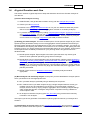
Quick start
Here are instructions to run the basic Zonation for those who have already familiarized themselves,
at least to some extent, with the program. For more detailed instructions and additional analyses
please see sections 3.2 Running Zonation, 3.3 Input files & settings, 3.5 Main analyses and 3.6
Post-processing analyses & options.
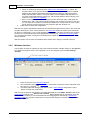
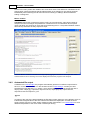
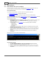
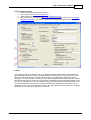
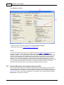
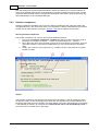
Using Windows interface
1. To run the program you need at least two sets of input files:
Species distribution map files, which are basic raster files (.asc) exported from GIS
programs. These files define species distributions in the landscape. The program can
incorporate any kind of species distribution data, such as presence-absence,
probabilistic or abundance data, or species-specific population connectivity surfaces
etc. Zonation v. 2.0 can also use point distribution data.
The names of all the species files must be listed in a separate species list file (.spp),
each file on a separate row with the species-specific parameters before the file name
(see section 3.3.2.2 Species list file for more detailed descriptions). The species list file
tells the program which species distribution files will be used in the analysis.
Remember to always use decimal points, NOT commas, in all input files!
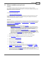
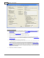
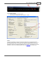
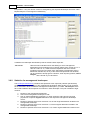
2.
Double clicking on the zig2.exe icon starts the windows version of the program.
3.
Go to Run settings -window and give the name of your species list file.
4.
Select the suitable cell removal rule.
5.
Give the name of your species list file.
6.
Define the name of your output files.
7.
Press Run -button to initiate the computation.
8.
For additional settings and analysis see sections 3.3.2.3 Run settings file and 3.5 Main
analyses. Features you might consider changing include the warp factor, the uncertainty
analyses and the aggregation methods.
9.
Note that using the windows interface is the secondary mode for running Zonation. Typically
runs would be started by calling batch files, which are simple text files that include a
Zonation call. Such runs are easily repeatable and less prone to parameter input errors than
the use of the interactive interface directly.
© 2004-2008 Atte Moilanen
9
Zonation - User manual
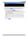
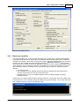
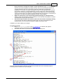
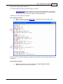
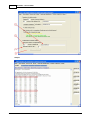
Using the command prompt
1. To run the program from command prompt, in addition to species distribution map files and
species list file you need a third input file called run settings file. This will define the setting
of your analysis.
2.
Select the suitable cell removal rule in your run settings file .
3.
Open the command prompt from your Windows "Start" -menu.
4.
Use "cd directory_name" -command to change to the correct working directory which
contains the zig2.exe and all the input and settings files. See section 3.9 for working with the
command prompt.
5.
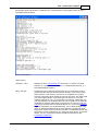
Call the program with the following command line:
call zig2 -r settingsfile.dat specieslistfile.spp outputfile.txt
0.0 0 1.0 0
In this command line, give the names of your settings file and species list file and define a
suitable name for your output files. See section 3.2.1 for explanations for the four numbers
in the call. Note that this call can also be written into a normal text file using notepad. If the
extension of the file is renamed to .bat (a batch file), the Zonation run can also be initialized
simply by double-clicking the file name in the Windows file manager. This is an easy way to
prepare and use batch files.
6.
Press enter to initiate the computation.
© 2004-2008 Atte Moilanen
Introduction
10
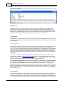
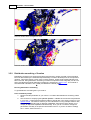
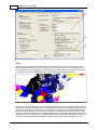
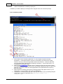
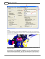
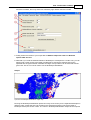
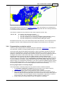
The basic Zonation program can be used for example for identifying a best proportion of the
landscape (rank selection in Map window), or for identifying the area required for representing a
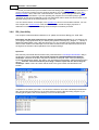
certain proportion of the species' distribution (remaining selection in Map window).
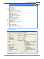
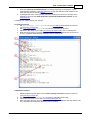
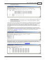
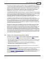
The program automatically produces six output files:
.jpg and .bmp maps of the landscape ranking showing the order cell removal in different
colors. See section 3.4.1 for detailed interpretation of the colors.
A .curves.txt -text file containing a list of species and weights used in the analysis, and
columns representing how large proportion of original occurrences of each specie is remaining
when landscape is iteratively removed.
A .rank.asc -raster file representing the order of cell removal (ranking). This file can be used to
produce map images in GIS softwares.
A .prop.asc -raster file representing proportions of species distribution (across species )
remaining at the removal of that cell. This file can be used to produce map images in GIS
softwares.
A .wrscr.asc -raster file. This file file contains a weighted range size normalized measure of
conservation value for each cell, which can be used as a scoring measure of value for cells.
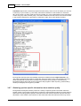
A .run_info.txt -text file copy of the Memo. This file will be created after you have closed the
program.
For saving other results (pictures of specific maps or curves), double click on the map image. See
also examples on visual output.
© 2004-2008 Atte Moilanen
11
1.6
Zonation - User manual
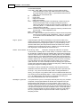
New features
This section shortly lists the new features and small additions that are included in Zonation v. 2.0 in
comparison to earlier versions. It also present some useful tricks you can use with Zonation.
Added for v. 2.0
Planning units As a new feature, Zonation can now be run with planning units larger than one
cell. With a specific planning unit layer you can group the cells in your grid into larger entities,
which will be removed as a whole instead of singular cells during the landscape ranking
process. These planning units can be of any shape and size. This option can be useful in
situation when, e.g., land ownership dictates that certain groups of grid cells should be treated
as distinct units.
SSI species A.k.a species of special interest. These are the second kind of species
occurrence information that can be entered into Zonation in addition to traditional species
distribution maps. The input for a SSI species is a (probably relatively short) list of observation
locations instead of a map. This option is particularly useful with species that have very few
occurrences and can not be modeled to produce a comprehensive distribution map.
New output Zonation v. 2.0 has new outputs: The species-specific habitat quality distribution,
which is displayed in the Species info -window, and the scoring measure for grid cell value,
which is produced together with the other output files.
New cell removal rule Cell removal rule number four is the generalized benefit function. This
is a two-piece power function which allows high flexibility in defining the shape and operational
features of the function.
Directed (freshwater) connectivity This is a development of the aggregation method
boundary quality penalty, with the distinction that the connectivity between sites is directed
(thus, it is not measured all around the cell as in BQP). This feature is particularly useful when
working with clearly directed systems, such as rivers.
Species interactions With this new feature species interactions, such as interactions between
prey and predator or host and parasite, can now be implemented to the landscape ranking
process. Thus sites can be valued not only by their importance to the target species, but also
how well they are connected to resources such as food, wintering areas etc.
Additional info in the Memo -window Because of all the cool features listed above, there is
a lot of new information printed into the Memo.
Facility for selecting top fraction of given cost Cost can now be used to calculate the
corresponding top fraction of the landscape. This new feature can be found in the Landscape
identification -window.
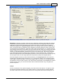
New outlook for run settings Because of all the new features, the outlook of run settings file
and window have changed quite a bit. Have a look!
Special maps New special maps are accessible via the Map -window. These include the old
richness and rarity maps, but also a planning unit map and river basin map, which indicates
linked planning units with the same color.
Addition to Curves output file If you have given conservation targets to your species (ie.
using target-based planning as your cell removal rule), the curves output file now tells you at
which level of cell removal process those targets for each species have been violated.
Implementing corridors Corridors can be designed by utilizing a combination of mask file use
and the BQP. Essentially, some good-quality areas are masked in to operate as the skeleton
of the corridor. Because the skeleton is masked in, and the BQP is used, it becomes
advantageous to expand areas around the skeleton. Whether the solution is good will very
much depend on the choice of skeleton areas, so they should be chosen well.
© 2004-2008 Atte Moilanen
Introduction
12
Outlook for the next version
V. 2.1 main feature: The main feature of v. 2.1 is going to be ability to use Zonation on
community modeling data, which utilize data/models about species richness and community
similarity/dissimilarity. Essentially, this builds an ability for the use of environmental-based
surrogates in Zonation. Look out for the new feature, which can be used in combination with
species-based analyses.
© 2004-2008 Atte Moilanen
13
Zonation - User manual
© 2004-2008 Atte Moilanen
Part
II
15
Zonation - User manual
2
Methods & algorithms
2.1
References
The basic Zonation analysis and distribution smoothing
Moilanen, A., Franco, A. M. A., Early, R., Fox, R., Wintle, B., and C. D. Thomas. 2005.
Prioritising multiple-use landscapes for conservation: methods for large multi-species planning
problems. Proceedings of the Royal Society of London, Series B, Biological Sciences 272:
1885-1891.
Moilanen, A. 2007. Landscape zonation, benefit functions and target-based planning: Unifying
reserve selection strategies. Biological Conservation, 134: 571-579.
Distribution smoothing, info-gap uncertainty analysis
Moilanen, A. and B. A. Wintle. 2006. Uncertainty analysis favours selection of spatially
aggregated reserve structures. Biological Conservation, 129: 427-434.
Basics of the information-gap decision theory and accounting for distributional uncertainty
Moilanen, A., Runge, M. C., Elith, J., Tyre, A., Carmel, Y., Fegraus, E., Wintle, B., Burgman, M.
and Y. Ben-Haim. 2006a. Planning for robust reserve networks using uncertainty analysis.
Ecological Modelling, 199 (1): 115-124.
Moilanen, A., B. A. Wintle, J. Elith and M. Burgman. 2006b. Uncertainty analysis for
regional-scale reserve selection. Conservation Biology, 20: 1688-1697.
A quantitative method for generating reserve network aggregation
Moilanen, A., and B. A. Wintle. 2007. The boundary-quality penalty: a quantitative method for
approximating species responses to fragmentation in reserve selection. Conservation Biology,
21: 355-364.
An extension of the BQP method to freshwater systems with different connectivity
requirements upstream and downstream
Moilanen, A., Leathwick, J. and J. Elith. 2007. A method for spatial freshwater conservation
prioritization. Freshwater Biology, 53: 577-592.
Accounting for species interactions
Rayfield, B., A. Moilanen and M.-J. Fortin. 2008. Incorporating consumer-resource spatial
interactions in reserve design. Submitted manuscript.
Replacement cost analysis
Cabeza, M. and A. Moilanen. 2006. Replacement cost: a useful measure of site value for
conservation planning. Biological Conservation, 132: 336-342.
See also the following references for the benefit function approach to reserve selection
Arponen, A., Heikkinen, R., Thomas, C.D. and A. Moilanen. 2005. The value of biodiversity in
reserve selection: representation, species weighting and benefit functions. Conservation Biology
, 19: 2009-2014.
Arponen, A., Kondelin, H. and A. Moilanen. 2007. Area-Based Refinement for Selection of
Reserve Sites with the Benefit-Function Approach. Conservation Biology, 21 (2): 527–533.
van Teeffelen, A., and A. Moilanen. 2008. Where and how to manage: Optimal allocation of
alternative conservation management actions. Biodiversity Informatics, 5: 1-13.
For those who would wish to familiarize themselves more broadly with recent literature concerning
spatial conservation planning, we recommend using Web of Science (or a similar search facility)
with key words such as, reserve selection, reserve network design, site selection algorithm,
area prioritization, spatial conservation planning and spatial optimization. Journals such as
Biological Conservation, Conservation Biology, Ecological Applications, Journal of Applied Ecology
and Environmental Modeling and Assessment, among others, include many studies concerning
quantitative conservation prioritization methods.
© 2004-2008 Atte Moilanen
Methods & algorithms
2.2
16
The Zonation meta-algorithm
The Zonation algorithm (Moilanen et al. 2005) produces a hierarchical prioritization of the
conservation value of a landscape, hierarchical meaning that the most valuable 5% is within the
most valuable 10%, the top 2% is in the top 5% and so on. At a high level, Zonation simply
iteratively removes cells one by one from the landscape, using minimization of marginal loss as the
criterion to decide which cell is removed next. The order of cell removal is recorded and it can later
be used to select any given top fraction, like best 10%, of the landscape. Simultaneously,
information is collected about the decline of representation levels of species during cell removal.
Essentially, the algorithm applied by Zonation is a reverse, accelerated, iterative heuristic. Reverse
comes from starting from the full landscape and removing cells (this is important for the treatment
of connectivity). Accelerated comes from the option of removing more than one cell at a time, via
the warp factor.
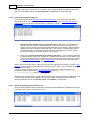
The Zonation meta-algorithm
1.
2.
3.
Start from the full landscape. Set rank r = 1.
Calculate marginal loss following from the removal of each remaining site i, i.
Complementarity is accounted for in this step.
Remove the cell with smallest i, set removal rank of i to be r, set r=r+1, and return to 2 if
there are any cells remaining in the landscape.
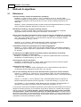
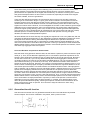
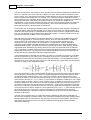
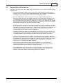
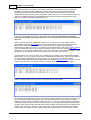
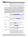
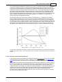
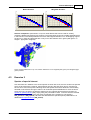
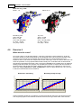
Thus, sites are ranked based on biological value and the least valuable cells are removed one (or
more) at a time, producing a sequence of landscape structures with increasingly important
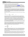
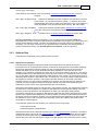
biodiversity features remaining. It is emphasized that the result of a Zonation analysis is not a
single set of areas. Rather, it is (i) the nested ranking of cells and (ii) a set of performance curves
describing the performance of the solution at the given level of cell removal.
1
0.8
0.6
0.4
0.2
0
0
0.1
0.2
0.3
0.4
0.5
0.6
0.7
0.8
0.9
1
proportion of landscape lost
Sample figures illustrating the ranking and the curves.
The Zonation meta-algorithm can, among other things, answer two questions frequently
encountered in conservation biology:
which parts of the landscape, totalling x% of landscape cost or area, have the highest
conservation priority (ranking), or,
which part of the landscape includes at least y% of the distribution of each species
(proportional coverage selection)?
Whether the Zonation algorithm makes any sense at all depends on the definition of marginal loss (
i), step 2 in the algorithm above. This definition is done by a separate cell removal rule, which is
described in the next chapter (see 2.3.). The Zonation method can thus be divided into two parts,
the Zonation meta-algorithm and the cell removal rule (= definition of marginal loss), which should
not be confounded. The cell removal rule should be seen as a separate component with several
alternatives that have different interpretations. Note that the notion of complementarity is inherent in
the way the cell removal rule is defined.
There is one feature, which according to Moilanen et al. (2005) is a part of the Zonation algorithm,
but which is more appropriately seen as a relevant detail for which there are alternatives. This is
© 2004-2008 Atte Moilanen
17
Zonation - User manual
edge removal, by which it is meant that cells can only be removed from the edge of the remaining
landscape. Edge removal may promote maintenance of structural habitat continuity in the removal
process. It also makes the cell removal process much faster with large landscapes, which is the
primary reason for using it.
2.3
The cell removal rule
This section is mainly based on Moilanen (2007).
The Zonation meta-algorithm is the same for all analyses described in this manual. The rule that
determines the loss of which cell leads to smallest marginal loss, and is therefore removed next,
differs depending on the cell removal rule that is chosen. There are three conceptually different cell
removal rules:
1.
2.
3.
Core-area Zonation
Additive benefit function
Target-based planning
In the following sections we first describe these three main cell removal rules and the theory behind
them, and then highlight the differences between the rules and give some guidelines how to choose
the most suitable one for your analysis. Finally we describe the fourth cell removal rule, added in
Zonation V2,
4. the generalized benefit function,
which is a two-piece power function that can assume very versatile forms, allowing flexibility in the
specification of conservation value.
Note that core-area Zonation has the property that it can identify important, otherwise species-poor,
locations where a single species has an important occurrence. The additive benefit function
analysis gives more weight to locations with high species richness. Therefore, it may be useful to
run both analyses and compare results. If the top-fractions do not agree, then there are some
species-rich areas but also some species-poor areas with occurrences of otherwise rare species.
Thus running both core-area Zonation and the additive benefit function analysis may reveal
information that is interesting for conservation planning.
2.3.1
Basic core-area Zonation
This section is mainly based on Moilanen et al. (2005) and Moilanen (2007).
In basic core-area Zonation cell removal is done in a manner that minimizes biological loss by
picking cell i that has the smallest value for the most valuable occurrence over all species in the
cell. In other words, the cell gets high value if even one species has a relatively important
occurrence there. The removal is done by calculating a removal index i (minimum marginal loss of
biological value) for each of the cells, where:
where wj is the weight (or priority) of species j and ci is the cost of adding cell i to the reserve
network. When running the analysis the program goes through all cells and calculates them a
value i based on that species that has the highest proportion of distribution remaining in the
specific cell (and thus represents the highest biological value to be lost, if the cell is removed). The
cell which has the lowest i -value, will be removed.
The critical part of the equation is Qij(S), the proportion of the remaining distribution of species j
located in cell i for a given set of sites (the set of cells remaining, S). When a part of the distribution
© 2004-2008 Atte Moilanen
Methods & algorithms
18
of a species is removed, the proportion located in each remaining cell goes up. This means that
Zonation tries to retain core areas of all species until the end of cell removal even if the species is
initially widespread and common. Thus, at first only cells with occurrences of common species are
removed. Gradually, the initially common species become more rare, and cells with increasingly
rare species occurrences start disappearing. The last site to remain in the landscape is the cell with
the highest (weighted) richness. This is the site that would be kept last if all else was to be lost.
Note that Eq. (1a) can alternatively be expressed as (Moilanen et al. 2005)
where qij is the fraction of the original full distribution of species j residing in cell i according to data,
and Qj(S) is the fraction of the original distribution of species j in the remaining set of cells S.
The min-max structure of the equation also indicates a strong preference to retaining the best
locations with highest occurrence levels. Thus, the program can spare otherwise species-poor
cells, if they have a very high occurrence level for one rare species. It is important to understand
that core-area Zonation does not treat probabilities of occurrence as additive; ten locations with
p=0.099 is not the same as one location with p=0.99. However, this is strictly true only when
analysis is based on biological value only and when a landscape cost layer is not used in the
analysis. When cost is used, cell removal is based on local conservation value divided by cell cost
(efficiency), and now a high value for a cell can be explained with either (i) a very high occurrence
level for some species or (ii) low cost for the cell. Thus, when cost information is used, the
interpretation of a core-area becomes vague, and this should be recognized in planning. Therefore
it is not recommended to use cost layers when trying to find out biologically most important areas
with core-area Zonation.
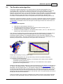
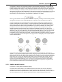
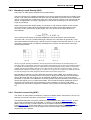
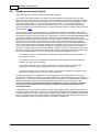
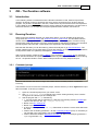
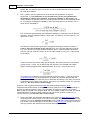
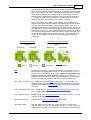
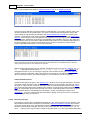
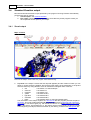
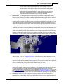
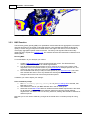
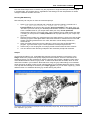
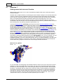
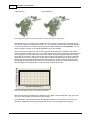
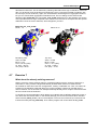
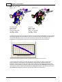
This figure illustrates principles that core-area Zonation implements in numerical form. Essentially, the
question is, if you have two (multiple) species, and you are going to lose a fraction (here one cell, marked as
yellow) of one distribution, then where would you prefer to lose the cell from? (A) If you have two otherwise
identical species, but one has a larger range remaining, then you prefer to lose from the species that has the
larger range. (B) If you have two otherwise equal species, but one has relatively higher weight, then you
prefer to lose from the distribution of the species with a lower weight. (C) You have two presently equal
species with equally wide distributions. Then you prefer to lose from the species that has had a smaller
historical reduction in the range (dashed line). (D) Within the distribution of a species, one prefers to lose
from a location with a relatively low occurrence density (light gray).
2.3.2
Additive benefit function
This section is mainly based on Moilanen (2007).
Compared to core-area Zonation, the additive benefit function takes into account all species
proportions in a given cell instead of the one species that has the highest value. The program
calculates first the loss of representation for each species as cell i is removed, and the i -value of
the cell is simply the sum over species-specific declines in value following the loss of cell i:
© 2004-2008 Atte Moilanen
19
Zonation - User manual
in which Qj(S) is the representation of species j in remaining set of sites S, and Qj(S-i) indicates
what remains after cell i has been removed. Here wj is the weight of the species j and ci is the cost
(or area) of planning unit i. Again the cell that has the smallest
-value, will be removed.
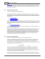
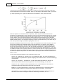
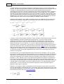
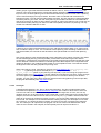
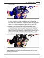
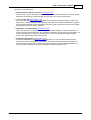
Above is a picture of a benefit function for species j. When a grid cell is removed from the
landscape, the representation of each species occurring in the removed cell goes down by a small
fraction Rj and the respective value for that species goes down by Vj. The total marginal loss in
value is simply a sum over species-specific losses. Note that here the species has a standard
weight of 1.0, but as with core-area Zonation it is possible to weight species differently when using
additive benefit function. The effects of weighting are seen on the scale of the y-axis which will go
from 0.0 to species weight wj instead of going from 0.0 to 1.0.
Because the additive benefit function sums value over all species, the number of species in a cell
has a higher significance compared to basic core-area Zonation. For example, using additive
benefit function might lead to situation where species-poor cells are removed even though they
have a high occurrence level for one or two rare species, because the i -value of these cells is
smaller than that for cells that have many common species with high representations. Thus, using
the additive benefit function typically results in a reserve network that has a higher performance on
average over all species, but which retains a lower minimum proportion of original distributions for
the worst-off species compared to core-area Zonation (see figure of the first three removal rules in
section 2.3.4).
To find more information about the use of benefit functions, see:
Arponen, A., Heikkinen, R., Thomas, C.D. and A. Moilanen. 2005. The value of biodiversity in
reserve selection: representation, species weighting and benefit functions. Conservation Biology
19: 2009-2014.
Arponen, A., Kondelin, H. and Moilanen, A. 2006. Area-based refinement for selection of
reserve sites with the benefit-function approach. Conservation Biology, 21: 527-533.
Cabeza, M. and A. Moilanen. 2006. Replacement cost: a useful measure of site value for
conservation planning. Biological Conservation,132: 336-342.
Moilanen, A. and M. Cabeza. 2007. Accounting for habitat loss rates in sequential reserve
selection: simple methods for large problems. Biological Conservation, 136: 470-482.
van Teeffelen, A., and A. Moilanen. 2008. Where and how to manage: Optimal allocation of
alternative conservation management actions. Biodiversity Informatics, 5: 1-13.
© 2004-2008 Atte Moilanen
Methods & algorithms
2.3.3
20
Target-based planning
This section is mainly based on Moilanen (2007).
Target-based planning is implemented in Zonation by using a very particular type of a benefit
function - the purpose of this special functional form is to enable the Zonation process to converge
to a solution that is close to the proportional coverage minimum set solution for the data. In this
function value Vj is zero until representation Rj reaches the target Tj. Then there is a step with the
height of (n+1), where n is the number of species. When Rj increases above Tj and approaches 1,
there is a convex increase in value, with a difference in value [Vj(1)-Vj(Tj)]=1. This means that the
loss in value from dropping any one species below the target is higher than any summed loss over
multiple species that stay above the target.
The idea is that, as cells are iteratively removed, species representations will approach the
species-specific targets from above, and that the convex formulation with increasing marginal
losses will force species to approach targets in synchrony in terms of lost value. Thus, as one of
the species approaches the target level, the program starts to avoid removing cells that contain that
particular species (at the expense of other species) in order to retain the target. At some point it will
not be possible to remove any more cells without violating the target for at least one species. After
one of the species has declined below target, the remaining distribution of that species has no
value for the reserve network. Thus removing cells where only this species occurs does not
increase the loss of biological value from network anymore.
Note however, that the definition of how marginal value is calculated does not change from that of
additive benefit function. Also with this cell removal rule species occurrences are considered as
additive and the cell that has the lowest marginal value summed across all species will be removed
next.
Also, when using target-based planning the species-specific weights have no function as the goal is
to retain a given proportion of distributions for all of the species. However, it is possible to set
different targets to different species. It is also recommended to avoid using very high warp factors
to allow the program to find the most optimal solution near the targets.
2.3.4
General differences between cell removal rules
It is important to realize that there may be significant differences between different cell removal rule
solutions and that the most preferable solution method depends on the goals of planning. Thus,
different cell removal rules may be conceptually better suited for different situations.
Core-area Zonation is most appropriate when there is a (i) definite set of species all of which
are to be protected - tradeoffs between species are discouraged, (ii) the hierarchy of solutions
and easy weighting of species is desired and (iii) importance is given to core-areas - locations
with highest occurrence levels; occurrences in cells are not additive meaning that twenty
locations with p=0.05 is not the same as one location with p=1.0.
The additive benefit function formulation may be more appropriate when (i) the species are
© 2004-2008 Atte Moilanen
21
Zonation - User manual
essentially surrogates or samples from a larger regional species pool, and tradeoffs between
species are fully allowed, and (ii) the hierarchy of solutions and easy weighting of species is
desired.
The targeting formulation is most appropriate when (i) it is accurately known what proportion
of the landscape can be had and the hierarchy is not needed, (ii) there is a definite set of
species all of which are to be protected, (iii) occurrences are additive, and (iv) easy weighting
of species is not needed. In target-based planning species weighting essentially needs to be
done by giving species different targets.
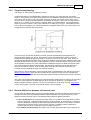
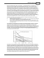
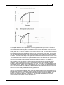
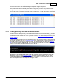
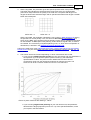
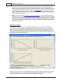
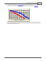
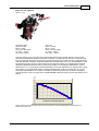
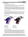
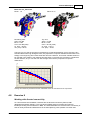
The figure above (from Moilanen 2007) illustrates some general differences between the core-area
Zonation, the additive benefit function formulation and the targeting benefit function. Here, the lines
show how large proportion of species distributions is remaining in the landscape as cells are
progressively removed. Overall, the additive benefit function has the highest average proportion
over all species retained (dashed line), but it simultaneously has the smallest minimum proportion
retained (solid line), because it favours species-rich areas over those areas that might be
significant for the existence of one species, but that otherwise are species-poor. Core-area
Zonation has a high minimum proportion combined with a relatively low average, because it retains
the most significant areas of species (the "core areas") till the end, even thought these areas might
be unsuitable for all the other species. The targeting benefit function does well in terms of finding
the highest level of cell removal without having any species-specific targets violated. However,
© 2004-2008 Atte Moilanen
Methods & algorithms
22
when further away from the target it does relatively poorly in terms of the minimum fraction over
species retained. The problem with the targeting benefit function is that it is aimed at good
performance at one particular set of targets, but the hierarchy of solutions is missing in the sense
that good overall performance at other levels of cell removal, especially at a level where targets
have been violated, cannot be guaranteed.
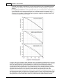
There are also differences between the cell removal rules on how much area they require for
achieving a set conservation target. To get a given minimum fraction across species core-area
Zonation requires more cells than the benefit function variants. This is because benefit function
variants take occurrences as additive whereas core-area Zonation prefers the locations with very
highest occurrence levels. However, if one investigates the number of cells needed to get the target
distribution for an individual species, then core-area Zonation may require fewer cells because it
prefers the higher-quality (density) cells. Thus, benefit function variants generate landscapes with
many species occurring simultaneously at potentially low occurrence levels and with high overlap
between species. Core-area Zonation produces solutions with species occurring at higher
densities, but with less overlap between species.
All these differences are such that they can logically be expected to occur in any data sets, with the
magnitude of differences depending on the nestedness of species distributions. Differences would
be largest when there are both (i) substantial regional differences in species richness and
occurrence levels combined with (ii) a generally low overlap between species distributions. In this
case core-area Zonation could catch cores of species occurring in species-poor areas whereas the
additive benefit function would concentrate the solution more towards species-rich locations, where
cells have high aggregate value over species.
Core-area Zonation and presence-absence data
Note that when using presence-absence data, all cells where a species is present receive an equal
value (of 1). Thus, in P/A data there apparently are no core-areas of particular importance for the
species, and it might seem pointless to use core-area Zonation as the cell removal rule. But this is
not the case. First of all, if you use any additional analyses such as aggregation methods or the
uncertainty analysis, the value of the cell will be calculated based on not only the species data, but
other features as well (e.g. connectivity of the cell). Thus, differences between areas where the
species is present do emerge. Secondly, even though in presence/absence data there are no core
areas in terms of relatively higher occupancy densities, there still is the significant difference in the
cell removal process between core-area Zonation and additive benefit functions. We highlight this
with an example. Let us assume we have a landscape where 7 different species occur. Six of these
species have overlapping distributions and one (denoted here as species A) has a distribution
isolated from the other species. Because benefit functions take species occurrences as additive,
the cells in sites where distributions of several species overlap receive a higher value than the cells
where only one species occurs, as is the case with species A. Thus, in the cell removal process the
additive benefit function would always favour cells with multiple species over the cells of species A,
which would lead to unequal preservation of species (in other words species A would loose its
distribution much more quickly than the other species). In contrast, Core-area Zonation would
retain all species distributions equally, meaning that species A would loose its distribution at the
same pace as do the other six species. This conclusion stays the same even when using
presence-absence data.
2.3.5
Generalized benefit function
Cell removal rule number four is a generalized benefit function form that allows very flexible
function shapes. The function is defined in two pieces, each a power function.
R
w1 j
Tj
V j ( R j ))
w1
© 2004-2008 Atte Moilanen
w2
Rj
x
if R j
Tj
1 Tj
Tj
y
if T j
Rj
1
23
Zonation - User manual
In this equation Rj is the fractional representation level of the species, the fraction of the original
distribution remaining. Tj is a nominal target level for the species, at Rj =Tj, the representation of the
species gets value w1. x is the parameter of the first part of the power function. When Tj < Rj < 1
the function continues as another power function with parameter y, and at Rj =1 the representation
of the species gets value w1+w2. Thus, by giving different values to parameters you have practically
an endless number of options for the shape of the benefit function. Note however, that the
definition of how marginal value is calculated does not change from that of additive benefit function.
Also with this cell removal rule species occurrences are considered as additive and the cell that has
the lowest marginal value summed across all species will be removed next.
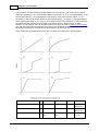
Some shapes that generalized benefit function can assume are listed in the following table:
w1
w2
Tj
x
Y
i) Linear
wj
0
1.0
1.0
NA,
dummy=1.0
ii) Power function (=ABF)
wj
0
1.0
<1 or >1
NA,
dummy=1.0
iii) Mild sigmoid
wj
same order
as wj
at inclination
point
>1
<1,
e.g. 1/x
© 2004-2008 Atte Moilanen
Methods & algorithms
iv) Steep sigmoid – step
imitation
wj
same order
as wj
at step
>>1
<<1,
e.g. 1/x
v) Ramp
wj
0
at step
1.0
NA,
dummy=1.0
vi) Ramp, with linear
over-representation
wj
<< wj
at step
1.0
1
24
The parameter definitions are suggestive, and the exact shape of the function can easiest be
determined by plotting it. To use generalized benefit function as a cell removal rule the parameters
of the function need to be given in the species list file.
2.4
Inducing reserve network aggregation
Fragmentation is an undesirable characteristic in reserve design as it has been concluded in many
studies that species persist poorly in small and isolated patches. Also, implementing a fragmented
reserve network may be awkward and expensive. In this section we introduce three different
aggregation methods that can be used when running analyses with the Zonation program. These
methods produce relatively more compact solutions. Note, however, that aggregation always
involves trade-offs. There is usually an apparent biological cost in more aggregated solutions
because in many cases it is necessary to include lower-quality habitats into the reserve network in
order to increase connectivity. In reality this apparent loss is more than offset by benefits of having
a well-connected area. Thus, it is recommended to use aggregation methods in reserve planning
as the cost of loosing a minor amount biologically valuable areas is usually low compared to the
benefits of high connectivity. For more information on true and apparent costs related to
aggregation, see Moilanen and Wintle (2006) and (2007).
There are some distinct differences between the aggregation methods in Zonation, and choosing
the right one depends on conservation targets and computational issues.
Boundary Length Penalty (BPL) has been the most commonly used way to introduce
aggregation to reserve planning. However, it is important to understand that BLP is a
general, non-species-specific aggregation method which does not asses the actual
effects of fragmentation on species. Rather the method only uses a penalty on a
structural characteristic of the reserve network (boundary length) to produce more
compact reserve network solution. The method is computationally quick and effective, but
might not be biologically most realistic.
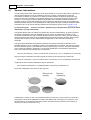
Distribution Smoothing is a species-specific aggregation method which retains areas
that are well connected to others, thus resulting a more compact solution. The
connectivity of sites is determined with a smoothing kernel, which means that the value of
a cell is "smoothed" to the surrounding area. Another way of looking at distribution
smoothing is, that it does a two-dimensional habitat density calculation, identifying areas
of high habitat quality and density. Consequently, cells that have many occupied cells
around them receive a higher value than the isolated ones. The widths of the smoothing
kernel are species-specific, implicitly expressing the species dispersal capability or scale
of landscape use. This aggregation method is computationally very quick. However, it
assumes that fragmentation (low connectivity) is generally bad for all species and it
always favors uniform areas over patchy ones.
Boundary Quality Penalty (BQP) is biologically the most realistic aggregation method
included in Zonation. This method describes how the local value of a site for a species is
influenced by the loss of surrounding habitat. The change in local value is based on
species-specific responses to neighborhood habitat loss, thus local value may also
increase if the site includes species that benefit from fragmentation. The downside of this
method is the required computation time, which is much higher compared to the other two
aggregation methods. This is because each cell removal influences the habitat value in all
remaining neighborhood cells, which needs to be accounted for in the cell removal
process.
Directed connectivity (Neighborhood Quality Penalty; NQP) is a generalization of
© 2004-2008 Atte Moilanen
25
Zonation - User manual
boundary quality penalty, where the connectivity between sites is strictly directed, such as
in riverine systems. This option also demands the use of planning units, groups of cells,
which are removed as a whole instead of singular cells during the landscape ranking
process. (In freshwater planning these units would correspond to catchments.) The value
of a focal planning unit is influenced by the removal of other planning units "upstream" or
"downstream" of the focal unit. Following the philosophy of BQP, also here the change in
local value is based on species-specific responses to nearby habitat loss. However, the
computation times are relative to the size of the planning units: Smaller planning unit size
means longer computation times and vice versa.
If you are including aggregation into your analysis, it is recommended to be careful with the
simultaneous use of multiple methods, due to difficulties in interpreting results.There however is no
technical reason why smoothing, the BLP and the BQP could not be used in the same analysis.
2.4.1
Distribution smoothing
This section is mainly based on Moilanen et al. (2005) and Moilanen and Wintle (2006). Instructions
to how to use distribution smoothing in Zonation can be found in section 3.5.2.
The first aggregation method described here is called distribution smoothing. When using
distribution smoothing, planning is based on a connectivity surface computed from the original
species distributions that have been input into zonation. The calculation that is applied to each
species distribution is identical to the calculation of a metapopulation-dynamical connectivity
measure, where the connectivity value is directly proportional to the number of migrants expected
at that location in the landscape. Technically, the computation is a two-dimensional kernel
smoothing using a species-specific parameter (width of the smoothing kernel).
For practical purposes, distribution smoothing identifies areas that have on average high
occupancy levels for species. The smoothing very effectively identifies important semi-continuous
regions where the species has overall high levels of occurrence, although not necessarily in every
grid cell. In contrast, relatively scattered occurrences in fragmented habitat lose value. As the
distribution of the species in the landscape becomes smoother, populations in fragmented areas
end up with less value relative to continuous areas with the same average probability of
occurrence.
Note that distribution smoothing should be used with care if the data includes a species that lives
happily as a metapopulation in a fragmented habitat - smoothing should be narrow for this species
at least if the habitat matrix is taken as partially suitable for the species. Distribution smoothing is a
convenient technique to apply because it can be run as a relatively fast preprocessing step before
going on to the zonation analysis itself. The appropriate level of smoothing for a given species
would be determined based on a conception of the typical dispersal distances for that species, or
from information concerning home range sizes for the species.
When using smoothing, the value for species j in a focal cell i is
where Oij is the original occurrence level of species j at cell i. Cell i is located in (u,r) and d(x-u, y-r)
is the distance between locations (x,y) and (u,r). The summation is over the landscape grid and j
is the parameter of the dispersal kernel for species j. This is a two-dimension kernel smoothing
using a radially symmetric negative exponential (dispersal) kernel.
2.4.2
Boundary Quality Penalty (BQP)
This section is mainly based on Moilanen and Wintle (2007). Instructions to how to use BQP in
Zonation can be found in section 3.5.3.
The boundary quality penalty is a quantitative species-specific way of inducing aggregation into
Zonation solutions. It can be seen as a way of approximating nonlinear effects of connectivity that
© 2004-2008 Atte Moilanen
Methods & algorithms
26
may be present in habitat models. The rationale behind the BQP goes as follows.
There are very many different statistical species distribution modeling techniques (a.k.a. habitat
models, resource selection functions, ...). Typically, in such models the abundance of a species at
a location is influenced not only by local habitat quality, but also by habitat in the neighborhood of
the location. Such a neighborhood influence essentially states that the species is somehow
dependent on connectivity or edge effects or both.
Now, ideally, reserve selection would be directly based on nonlinear habitat models with
neighborhood effects. However, this is not realistically possible, because it would make reserve
selection computationally very, very slow. Also, implementing dozens of different habitat modeling
techniques efficiently into reserve selection software would be an enormous task. Herein enters the
BQP.
The BQP is a mechanism for approximating the aggregate response of a species to edge effects
and metapopulation size and connectivity. It can be seen as a way of exploiting the connectivity
response that is present for a species in a habitat model. Essentially, one uses the habitat model
for two things. First, one predicts an abundance or probability of occurrence into every cell in the
landscape – giving the standard input layer for one species. Additionally, one analyses the habitat
model to find out what kind of an aggregate response to habitat loss and fragmentation does the
species have. And this response is transferred into Zonation as a standardized curve, which
mediates the boundary quality effect in Zonation.
Different species can have different responses to fragmentation and habitat loss, which are entered
into Zonation as two BQP components: (i) a species-specific radius and (ii) a response curve. First,
the radius. The effect of habitat loss can be localized (the species only has a narrow edge effect or
so), or, the effects can extend over a longer distance, as could be the case with a timid larger
animal that avoids human proximity – habitat loss could negatively influence such a species from a
long distance away. By setting a species-specific radius, one can model how close habitat loss
influences the species. Note that inside the radius only the loss of those cells that have data on the
particular species (in other words cells that are not marked as missing data) can influence the
value of the focal cell.
Figure clarifying the two components used when specifying the BQP for a species.
© 2004-2008 Atte Moilanen
27
Zonation - User manual
The second component, the response curve, specifies the kind of effect neighborhood habitat loss
has on the species. First, there could be an absence of effect, which would be modeled by a flat
line (no effect). Then, the species could suffer variable degrees of loss in local population density if
there is neighborhood habitat loss. For example, you could have a relatively insensitive species,
which loses half of the population density when the focal cell has lost all it neighbors from inside the
species-specific buffer. Then again, the species could be very sensitive to neighborhood
fragmentation – all local value could be lost when only half of the neighboring cells have been lost.
And finally, a species could even favor fragmentation, which would be modeled by a response
curve that goes above 1 at some levels of habitat loss.
For the exact way of analyzing a habitat model to get the species-specific response, see Moilanen
and Wintle (2007). Note also that the BQP curves need not be derived from habitat models. One
could also use expert opinion to guesstimate the response of the species to neighborhood habitat
loss. The hypothetical curve would then be entered into Zonation – it makes no difference for the
Zonation process how the BQP-curves were obtained.
Note that there are major differences between distribution smoothing and the BQP even though
both induce aggregation in a species-specific manner. First, from a practical point, the BQP is
much slower to run as the effect of removing a cell is not only local but extends over the
neighborhood area which needs to be accounted for in computations. Second, the BQP is
biologically better justified. The BQP definitions can be based directly on species responses in
statistical habitat models. The difference between the methods would be most strikingly visible in
fragmented areas. Distribution smoothing perceives the value of fragmented areas as relatively
low. In comparison, the BQP could recognize a species that happily lives as a metapopulation in a
fragmented environment – the response for that species would be such that it is recognized that
the species can have high-value habitats in fragmented areas.
In the implementation of the BQP into Zonation, the value of a cell that is removed is now divided
into two components (i) local value, which is as before, and (ii) loss of conservation value in the
neighborhood of the focal cell as modeled via the BQP specification. Thus with BQP the effect of
cell removal is not only the loss of the value in the cell itself but also a (potentially species-specific)
reduction in quality in the neighborhood cells:
,
where Nj(i) indicates the cells (containing data for that species) within the species-specific radius of
cell i for species j. Denoting by h the fraction of original neighbors that have been lost from within
the species-specific buffer around the site, Hj(h) is the proportion of the original value of cell k
remaining for species j when the focal cell has fraction h of its neighbors remaining. The fraction of
cells remaining is simply h = nkj /nkj*, where nkj is the number of neighbors remaining for cell k within
the buffer radius of species j, and nkj* is the original number of neighbors. The loss term in the curly
brackets is divided into two, local loss and loss in the neighborhood of the focal cell. Local loss is
the fraction remaining of the original value of the focal cell i - if many of its neighbors have already
been lost, the value of Qij(S) has been reduced. Loss in the neighborhood is mediated via the loss
of one cell from the number of neighbors, which goes down from nkj to nkj - 1. (Note that the formula
above is employed as it is only for the core-area Zonation. For additive benefit function and
target-based planning the formula includes few trivial differences, but the concept behind BQP is
the same in all cases.)
The size of the neighborhood of a cell and the effects of habitat loss are defined separately for
each species according to habitat models, which themselves mediate the boundary quality penalty.
Because BQP ranks the cells based on the responses of species to fragmentation, also species
that actually benefit from the loss of surrounding habitats will be equally protected (compare
distribution smoothing).
© 2004-2008 Atte Moilanen
Methods & algorithms
2.4.3
28
Boundary Length Penalty (BLP)
This section is mainly based on Moilanen and Wintle (2007).
The most common way of adding aggregation into a reserve network has been the boundary length
penalty. This method is qualitative in the sense that the estimated conservation value of individual
cells, or consequently the conservation value of the entire reserve network, is not influenced by the
degree of fragmentation, but rather, aggregation is induced via a penalty given for the boundary
length of the reserve.
When using the boundary length penalty, the hierarchy of cell removal is based on both species
occurrence levels in cells and the increase/decrease of boundary length that results from the
removal of a cell. The boundary length penalty can in the context of core-area Zonation be
formulated as:
where (BL/A) is the change in boundary length/area -ratio of the reserve network following
removal of cell i, and is a constant defining the strength of the boundary length penalty. If cell
removal decreases boundary length, (BL/A) receives a negative value and the value of i for cell
i decreases, indicating that it is relatively advantageous to remove the cell because removing it
reduces fragmentation.
L=0
L = +2
L = -2
Above is a picture showing how different cell removal options would influence the boundary length. The
boundary length is calculated in the terms of cell edges. Removing the gray cell in the first example results in
no changes in boundary length for as two edges are removed while another two are gained. In the second
example the cell removal leads to the loss of one edge, but also to the gain of three new edges. Thus as a
result the total change in boundary length is +2, and so on. To get from L to (BL/A) one needs to account
for both the change in boundary length and the decrease of the reserve area by one.
Note that BLP is different from both distribution smoothing and the BQP. First, the BLP is not a
species-specific way of handling reserve connectivity. It simply uses a penalty term that devalues
reserve structures with lots of edge. This is completely qualitative; there is no species-specific
parameter or response. Like distribution smoothing, the BLP may be expected to perform poorly for
species that happily occur in fragmented habitats. This is because the BLP qualitatively favours
structurally connected areas, and it will therefore have a tendency to remove small habitat
fragments from the solution irrespective of whether some species can actually persist in them or
not.
2.4.4
Directed connectivity (NQP)
This section is mainly based on Moilanen, Leathwick, and Elith (2008). Instructions for how to use
directed connectivity in Zonation can be found in section 3.5.4.
The directed freshwater connectivity measure is a generalization of the BQP technique, in which
the concept of neighborhood is generalized – hence the name Neighborhood Quality Penalty
(NQP). Instead of using a circular neighborhood, the NQP is defined using a tree-hierarchy of
linked planning units. A focal area (planning unit) is influenced by negative action (habitat loss)
potentially both “downstream” and “upstream” from the focal location, depending on the
requirements of the species.
© 2004-2008 Atte Moilanen
Zonation - User manual
29
The NQP technique was originally developed for freshwater planning in riverine systems. Note
however, that the technique could be suitable for quite different situations as well: the NQP method
is based on a bidirectional linking of planning units. These linkages could correspond to
hydrological flow. But, they could also correspond to other kinds of biological linkages, including (i)
other spatially continuous connecting landscape elements, such as hedge rows, or (ii) spatially
discontinuous functionally linked planning units, such as areas on migration routes of birds, or (iii)
they could approximate connectivity at marine areas where very strong flows generate a situation
analogous to a river system. In the end, an appropriate aggregation of cells to planning units and
suitable linkages and loss functions allow modeling of relatively variable situations.
Following closely Moilanen et al. (2008), the present version of the NQP technique is technically
specified by the following modification of the marginal loss value used in the cell removal rule:
ij
local
ij
neighborhood
ij
local
ij
upstream
ij
downstream
rijup down rijdown
hj
oijup
oijdown
up
ij j
ph
pkj h
up
j
k N iju p
pkj h
k N ijdown
up
j
rkjup down rkjdown
hj
okjup
okjdown
rkjup down rkjdown
hj
okjup
okjdown
h
up
j
h
up
j
rkjup down rkjdown Aij
hj
okjup
okjdown
rkjup Aij down rkjdown
hj
okjup
okjdown
.
(1)
in which pij is the occurrence level of species j in cell i. Equation (1) describes the fraction lost from
original distribution of species j following the removal of site i. The loss consists of three
components, local loss, loss upriver, and loss downriver. The assumption is that everything
remaining locally is lost if a cell is removed, and that loss accrued upriver and/or downriver will
depend on the size of unit i for species j, Aij – loss of a larger unit implies greater influence on
connectivity nearby. The influence of connectivity on occurrence levels is mediated via functions hj
(upriver and downriver), which are response functions like those in BQP with the x-axis reversed.
When the full landscape remains, and nothing has been lost, hj (1)=1. Importantly, when calculating
marginal loss, the equation accounts for degradation that already has occurred. This implies that if
no local value remains due to past neighborhood loss, further loss of connectivity has no local
influence on the species.
Connectivity in Eq (1) is modeled separately upriver and downriver. Quantities rij and oij (up and
down) are the remaining and original connectivities of unit i for species j both upriver and downriver,
respectively. Loss of planning unit i influences the downwards connectivity of sites upriver from it,
which is the component of the equation having the summation across neighbors k upriver from
focal site i, k Nijup. Similarly, loss of unit i influences the upwards connectivity of units downriver
from it. Note that the present version of Zonation uses species and unit specific predictions of
occurrence pij and species-specific connectivity responses hj(). However, connectivity up and down
is based directly on the numbers of grid cells in planning units in a non-species-specific manner,
meaning that rij, oij and Aij are taken as the same for all species, which assumption might be
relaxed in a later version of Zonation.
Equation (1) is simply the fraction of distribution lost for one species, which does not account for
how lost representation is translated to lost in conservation value. When deciding which cell can be
removed with smallest loss of conservation value, ij is aggregated across species according to the
cell removal rule, which now is for core-area Zonation
(2a)
© 2004-2008 Atte Moilanen
Methods & algorithms
30
and for the additive benefit function Zonation
(2b)
in which wj is weight of the species j, ci is cost (or area) of planning unit i, and qj is the fraction of
distribution of species j remaining before removal of cell i, and Vj() is the function translating
increasing representation into increasing conservation value (see Sections 2.3.1 and 2.3.2;
Arponen et al. (2005); Moilanen (2007)).
© 2004-2008 Atte Moilanen
31
2.5
Zonation - User manual
Uncertainty analysis
A common problem with conservation planning is the uncertainty of planning inputs. Mostly these
uncertainties are due to lack of data - we simply do not have a comprehensive database with
accurate information of the distribution of every species. Uncertainty can also arise, for example,
from outdated or false observations, the use of predicted data (e.g. distribution models), or from
any future factors such as the potential for anthropogenic land-use changes, or climate change.
Taking into account both biological value and uncertainty creates a prospect of four scenarios. (1)
Areas with high conservation value and high certainty of that information would be important for
conservation. (2) Areas with low conservation value and high certainty (car parks, etc.) would
ordinarily rank low among conservation priorities. (3) Areas with high estimated conservation value,
but low certainty have potential for producing negative surprises for conservation. (4) Finally, areas
with low conservation value and also low certainty have potential for producing positive surprises.
The goal of uncertainty analysis in reserve selection is to implement and evaluate trade-offs
between biological quality and the certainty of that information. Ideally, one would identify a reserve
network that guarantees high biological quality despite some uncertainty in input data. Uncertainty
analysis could also be used for evaluating the opportunities arising from uncertainty, that is,
potential for positive surprises.
Here we introduce two methods of uncertainty analysis that can be used in the Zonation context.
The first method is called distribution discounting, which enables the ranking of the landscape
using species distribution data that includes uncertainties. Our second method is for testing reserve
network structures to see how robust they are against uncertain negative influences of habitat loss
and fragmentation.
For more information about the aims and methods of uncertainty analyses in reserve selection,
see:
Moilanen, A., Runge, M. C., Elith, J., Tyre, A., Carmel, Y., Fegraus, E., Wintle, B., Burgman, M.
and Y. Ben-Haim. 2006. Planning for robust reserve networks using uncertainty analysis.
Ecological Modelling 199: 115-124.
Moilanen, A. and Wintle, B.A. 2006. Uncertainty analysis favours selection of spatially
aggregated reserve structures. Biological Conservation 129: 427-434.
Moilanen, A., Wintle, B.A., Elith, J. and Burgman, M. 2006. Uncertainty analysis for
regional-scale reserve selection. Conservation Biology 20: 1688-1697
2.5.1
Uncertainty in species distributions, distribution discounting
This section is mainly based on Moilanen et al. (2006). Instructions for how to use distribution
discounting in Zonation can be found in section 3.5.5.
Distribution discounting is a method for including uncertainty analysis into the conservation
prioritization done in Zonation. This method helps you find the most robust solutions, those that
© 2004-2008 Atte Moilanen
Methods & algorithms
32
most likely achieve a conservation goal given a level of uncertainty in species distributions. This
analysis utilizes both the estimated biological value (probability of occurrence) of a species in a cell,
and the certainty of that information.
Looking for robust reserve networks
In the framework of uncertainty analysis, one goal for reserve selection would be to find those
network candidates that would achieve the given conservation targets despite uncertainty in input
data. Thus, cells need to be ranked so that the highest priority is given to cells that have both
relatively high conservation value and high certainty of information. In Zonation, uncertainty analysis
has been implemented according to a convenient formulation that uses information-gap decision
theory (see Ben-Haim 2006).
Conceptually, relevant components of the info-gap theory are
1.
The nominal model. This is your best set of predictions for species.
2.
The uncertainty model. This states that even though you do have a nominal estimate,
your true probabilities of occurrence are certain to deviate from your nominal model. The
uncertainty model specifies a set of bounds that expand around the nominal estimate as a
function of an uncertainty parameter, .
3.
A performance function. This is a function measuring how well you are doing, for
example, what is the proportion of species distributions that would be covered by a given
set of areas.
4.
Robustness function. This function measures "how large can the horizon of uncertainty
be so that conservation goals are still met even if you take the most adverse choice of
probabilities from inside the uncertainty bounds". A good reserve candidate is such that it
achieves goals while allowing for high uncertainty ( ). The robust optimal reserve
candidate is the one that achieves conservation goals while allowing for highest
uncertainty.
Ben-Haim, Y. 2006. Info-gap decision theory: Decisions under severe uncertainty, 2nd edition.
Elsevier Academic Press.
At simplest, distribution discounting is implemented as follows
1. Take your nominal estimates (the normal input distributions for species)
2. Develop a respective uncertainty map for each species. The uncertainty layer could, for
example, represent the standard deviation (SD) of the nominal estimate or the length of the
lower half of the 95% confidence interval.
3. Specify, e.g., that the horizon of uncertainty is 0.5 or 1. E.g., if = 1 and your uncertainty
model is 1xSD, then you would essentially subtract one SD of the nominal estimates, thus
emphasizing locations with relatively certain predictions.
© 2004-2008 Atte Moilanen
33
Zonation - User manual
Distribution model
Error surface
Discounted distribution
Picture demonstrating the concept of distribution discounting. Here the first picture shows a modeled map of
species distribution, white areas representing a high probability of occurrence. The second picture displays
an error surface, eg. standard deviation of the modeled values, again white color indicating large deviation
and therefore high uncertainty. The -value (horizon of uncertainty) can be used to either enhance or
diminish the strength of the error surface, e.g. = 2 would double all error values in the map. The third
picture is species discounted distribution, where the error surface has been subtracted from the modeled
distribution map. This is the map that Zonation finally uses to run the analysis.
An expanded explanation for distribution discounting.
In more detail: The occurrence of species s in a cell c (here indicated as p*sc) is by no means
certain, but merely the nominal "best guess" probability. Thus the true probability psc [0,1] could
be within an interval given by:
where is the horizon of uncertainty and wsc is any error measure related to the accuracy of p*sc
(for species s in cell c). Thus the true probability psc could be either higher or lower than the
estimate p*sc, with bounds for psc determined by and the relative error measure wsc, which could
be, for example, related to the accuracy of statistical prediction. The model of Eq. (1) is called an
uniform bound model in info-gap terminology.
When using predictions based on logistic regression habitat models, a plausible model for
uncertainty is to define the uncertainty interval in logit space, where wsc is the standard error for the
linear predictor of a logistic regression:
According to info-gap theory, one should favor reserve structures that achieve given conservation
targets even with the most adverse choice of probabilities (in other words, in the worst case
scenario). Given the present definitions, the most adverse choice of probabilities occurs when all
probabilities are at their lower bounds (this is when the lowest expected number of populations is
obtained). Assuming the analysis in logit space:
Thus the program calculates the discounted biological value of a cell by reducing (discounting) the
value of the logit of probability (p*sc) by a multiple of the error ( wsc). In the distribution discounting
technique, the original estimated occurrence data is simply replaced by the discounted data before
proceeding to do the Zonation run. Thus, one Zonation run with discounted data is needed for each
value of the horizon of uncertainty, . Note that Zonation does not care how the nominal estimates
and associated error measures are obtained - any statistical method or expert evaluation can be
used as a basis for developing those quantities.
© 2004-2008 Atte Moilanen
Methods & algorithms
34
But how to determine the horizon of uncertainty, ? As mentioned above, the relative error wsc can
be any error measure related to the predicted species distribution. It can, for example, be a
statistical error (e.g. the length of the lower half of the 95% confidence interval) or a probability of
future anthropogenic threat, or both. The value of , on the other hand, is unknown and has no
correct value. The way forward is to investigate how different reserve network candidates perform
under increasing uncertainty. In practise, the way is to try out several levels of to see what areas
are selected. If an area is always selected irrespective of the value of , then the area is important
for sure. If the area is selected with low but not with high alpha, then the area is selected because
of the occurrence of an uncertain biological feature. If the area is not selected with low but is
selected with high alpha, then something of interest occurs in the area with relatively low density
but high certainty. Based on such uncertainty analysis, one can split the landscape in three
categories of areas: (i) areas that are good for sure, (ii) areas that are never selected and thus
have low priority and (iii) areas that are selected with some levels of uncertainty - these areas may
need further investigation before a choice of conservation priority for them can be fixed.
Distribution discounting uses the following algorithm for finding robust-optimal reserve designs:
1.
Specify robustness requirement .
2.
Distribution discounting. Read in species information. For every species and cell, apply Eq.
(3) or its analogue, depending on type of data/uncertainty model.
3.
Use any reserve selection algorithm (here Zonation) to search over spatial patterns. The
robust optimal design X* (at the given level of ) is the one achieving the highest possible
conservation value.
The advantage of this approach is that the worst-case probability set (Eq. 3) has to be calculated
only once (item 2.), and thereafter the contributions of cell to representation levels, psc, do not
change in the reserve selection process. Testing several -values allows you to outline how
different reserve structures behave in increasing uncertainty. Some designs are always bad, some
are good according to nominal habitat model predictions, but bad if uncertainty is incorporated into
the models. Others have intermediate nominal performance, but have a good robustness to
uncertainty. The robust-optimal designs are always at the Pareto-optimal boundary with respect
to the target, as demonstrated below:
Here each thin line represents one solution (spatial reserve structure). An increasing robustness
requirement ( ) implies that a decreasing biological value can be achieved reliably. The thick line is
the Pareto-optimal boundary representing solutions that are optimal in the sense that increased
biological value can only be obtained with the cost of lowered robustness, and vice versa. When
doing reserve selection on a large grid, there is a huge number of potential reserve structures, but
only one or few of them would correspond to the Pareto-optimal boundary at any given -level and
resource (fraction of landscape). Any solution not at the Pareto-optimal boundary is inferior in the
sense that another solution exists with either higher biological value or higher robustness or both.
The distribution discounting technique used inside Zonation automatically identifies the
robust-optimal nested Zonation set of solutions for the given level of .
© 2004-2008 Atte Moilanen
35
2.5.2
Zonation - User manual
Uncertainty in the effects of landscape fragmentation
This section is mainly based on Moilanen and Wintle (2006). Instructions of how to use
fragmentation uncertainty analysis in Zonation can be found in section 3.6.4. This analysis is for
investigating how robust a given reserve network is to potential negative effects of fragmentation.
This is a minor analysis that would not be relevant for most applications of Zonation - essentially, it
is intended for the investigation of the robustness of a network that has been designed without any
spatial aggregation method. The description below is a brief description of the analysis, please see
the original publication for details.
We start from the assumption that cells ending near the edge of a reserve network will end up with
decreased conservation value due to negative edge effects, disturbance and disrupted spatial
(meta)population dynamics. Just like distribution discounting, fragmentation uncertainty analysis is
based on the info-gap theory. Since the main interest of this analysis is uncertainty in conservation
value due to habitat loss and fragmentation, error rates (see section 2.5.1) are explicitly related to
the amount of habitat loss occurring near the focal cell, assuming the habitat close to the reserve
network border is degraded.
The error model chosen for this study specifies that the "true" value of a cell is inside an uncertainty
interval;
where the relative error measure wsc has been replaced by the proportion of cells lost from the
neighbourhood of focal cell c, Lc. (This is the proportion of cells that were available but were not
chosen into the reserve network.) The uncertainty model above is a proportional error model in the
info-gap terminology (Ben-Haim, 2006). In the equation, f( Lc) could be any decreasing function of
Lc with f(0)=1, and f(x) (0,1) for all x 0. The condition f(0)=1 specifies that if nothing has been lost
from the neighborhood of a cell, then the nominal predictions should be used as there is no
uncertainty caused by nearby habitat loss. In the Zonation program a simple relationship f( Lc
)=exp(- Lc) is used, but any other decreasing function would give similar results. With this
relationship, if =0 (no uncertainty) or if there is no habitat loss (Lc=0), then from (1) it follows that p
sc=p*sc. Increasing the uncertainty parameter
or the fraction of habitat lost will result in a potential
loss of conservation value in the target cell.
Note that it is not claimed that any correct value of is known. Rather, the uncertainty analysis will
proceed to analyse how robust different solutions (reserve network candidates) are to increasing
uncertainty. The second component needed for the uncertainty analysis is a measure of the
performance of a candidate reserve network as uncertainty is increased. The performance of
species s in candidate reserve network X, Vs(X,p), was defined as the proportion of the original full
distribution of the species remaining in the given reserve structure X;
where p*sc is the original value for species s in the cell c, and psc is the final value after the loss of
neighbourhood habitat has been taken into account. xc receives values depending whether the cell
in question is included to the candidate reserve network (xc=1) or not (xc=0). Just like in distribution
discounting, also here the evaluation of robustness means that we are interested in the most
adverse choices. Therefore, we look at the lower bounds of probabilities. This means that in Eq.
(2) psc is equal to f( Lc)p*sc.
Different reserve structures will be differentially resistant to negative effects of fragmentation - very
fragmented reserve networks will have the characteristic that if species occurring in the network are
sensitive to fragmentation, then the true value of the network can be much less than what is
estimated based on an analysis that does not include explicit spatial effects. In contrast, a large
© 2004-2008 Atte Moilanen
Methods & algorithms
36
and well-connected reserve will be relatively insensitive to negative effects of fragmentation,
because only a small fraction of the reserve area will be close to the reserve edge. Essentially,
such a reserve would have a large core. When running the fragmentation uncertainty analysis, the
program calculates how much biological value might be lost from a candidate reserve network as
the uncertainty and/or the fragmentation of surrounding habitats increases (see section 3.6.4).
© 2004-2008 Atte Moilanen
37
2.6
Zonation - User manual
Replacement cost analysis
This section is mainly based on Cabeza and Moilanen (2006).
Very seldom can reserve planning be started from a fresh table with areas that have no older
reserves nor any restrictions for conservation (such as areas ear-marked for residential building).
More commonly reserve networks are planned so, that due to logistic or social constraints, certain
sites need to be included to, or excluded from the final solution. In most cases this leads to a
suboptimal network either in terms of conservation value or in terms of the cost of achieving a
given conservation goal. Instructions how to include or exclude areas to a Zonation solution can be
found in section 3.5.7.
It is useful to be able to asses the degree of suboptimality of solutions compared to the optimal
ones. Here we introduce a method called replacement cost analysis, which can be used to evaluate
the effects of forced site inclusion/exclusion. Replacement cost refers to the loss in solution value
given that the optimal cost-efficient solution cannot be had and that alternative solutions, with
particular sites forcibly included or excluded, must be accepted. It tells us at what cost (biological or
economic) can we exclude (or include) a site from the reserve network. Assuming a constant
budget, the exclusion cost of that site is the loss in the network's conservation value that follows
when a site that belongs to the optimal solution cannot be taken. The inclusion cost of a site is the
loss in conservation value that must be accepted if a suboptimal site is forced into the reserve
network. On the other hand, when the conservation budget is not fixed, replacement cost can also
be defined in terms of the extra funding required to maintain conservation value that is equal to the
value of the optimal solution. Thus, one can define four variants of replacement cost:
1. Biological exclusion cost. Decrease in conservation value following forcible exclusion of a
given (group of) site(s).
2. Biological inclusion cost. Decrease in conservation value following forcible (suboptimal)
inclusion of a given (group of) site(s).
3. Economic exclusion cost. Increase in solution cost required to keep the same total
conservation value following the forcible exclusion of a given (group of) site(s).
4. Economic inclusion cost. Increase in solution cost required to maintain conservation value
following the forcible inclusion of a given (group of) site(s).
For practical purposes, the replacement cost is calculated in the following manner. First, find
optimal reserve selection X* which has highest possible value F(X*) obtainable with the available
resource (Cmax). Then rerun the analysis with some areas forced in or out. Replacement cost is the
difference between the value of the optimal solution and the value of the new solution. We
emphasize that this does not mean keeping the optimal set of sites plus/minus a particular
site, but finding a completely new solution given that the particular site(s) are forcibly
included/excluded.
A replacement cost of zero tells us that there exists an alternative solution with the same value as
the current (best) solution has, i.e. same cost, and same conservation value (although obtained via
a different selection of areas compared to the original optimal selection). A replacement cost larger
than zero means that any alternative solution including/excluding the focal site(s) will have either a
lower conservation value or a higher economic cost than the optimal one.
© 2004-2008 Atte Moilanen
Methods & algorithms
38
A conceptual illustration of the replacement cost of a hypothetical site (a) in terms of increase in
resources required to maintain value ( C) and (b) in terms of loss of biodiversity value ( F) (from
Cabeza and Moilanen 2006). (a) Exclusion cost: the dashed line indicates the value of the best
solution when site x is forcibly excluded. Up to a certain resource level, CE,k, site x does not belong
to the optimal solution and thus exclusion cost is zero. Even with C>CE,k, exclusion cost can be
zero if the site is fully exchangeable with another site or a combination of other sites. (b) Inclusion
cost: the dashed line indicates the value of the best solution when a site is forced to be included in
the solution. Inclusion cost is likely to be highest with low resource, when the forced inclusion of the
unwanted site prevents the acquisition of other biologically much more valuable locations. At C>CI,k
, the focal site becomes included in the optimal set and inclusion cost becomes zero. (Note that the
resource here should be understood the proportion of landscape retained in the Zonation.)
The figure also shows an example of how exclusion and inclusion can be expected to behave
qualitatively. With a small resource (<CE,k), the exclusion cost (a) of a site is likely to be zero,
because the site would not be in the optimal set in any case. At a level CE,k the site becomes part
of the optimal solution. With a resource slightly higher than CE,k, it is likely that the exclusion of the
site can be compensated with small cost, at least if there are many selection units. However, when
the available resource is large, sites of less importance are included in the solution and the
exclusion of a high-quality focal site has a clearly positive cost.
Inclusion cost (b) behaves differently. When a site that would not belong to the optimal solution is
included in the network it generates an increase of cost even when the resource available is small
because the resource is spent on suboptimal areas. With increasing resource availability, the
inclusion cost gradually decreases. At a level CI,k, the site would already become part of the
optimal solution and inclusion cost thus becomes zero.
© 2004-2008 Atte Moilanen
39
2.7
Zonation - User manual
Species interactions
In most cases conservation planning is done purely based on occurrence data, either of species or
other biological features such as vegetation types etc. However, sometimes more specific
information is needed, for example, if we want to include interactions between species and e.g.
their food resources, predators or competing species, into conservation planning process. With
Zonation v. 2.0 this type of specific planning is possible as the software includes a facility for
modeling a variety of species interactions. In this section we describe the method and philosophy
behind this facility and give some possibilities of cases where this type of analysis would be useful.
Instructions for how to include species interactions into Zonation can be found in section 3.5.6.
(1) Interaction type 1 - resource-consumer, predator-prey, host-parasitoid, present to future
distribution, etc. type interactions.
The general idea is that one wishes to (i) protect the resource independently, (ii) protect a part of
the resource distribution which is available to the consumer, (iii) emphasize protection of the
consumer at areas that are within foraging distances from the resource. Item (i) can be achieved
simply by entering the resource as an independent layer into the Zonation analysis. Items (ii) and
(iii) are linked, and they can be implemented via application of the distribution smoothing
technique.
The figure below illustrates the principle of positive connectivity interactions in Zonation (see
Rayfield, Moilanen, Fortin, submitted). There are four distributions of interest, the first two of which
are not interaction layers: i) the distribution of the resource (prey, host etc.), and ii) the distribution
of the consumer (predator, parasitoid). The two other distributions are interaction distributions.
First, iii) the resource use intensity layer is defined as
resource use intensity = (local occurrence level of resource) x (con. to distribution of consumer)
and iv) turning the interaction around one gets the resource connectivity layer, defined as
resource connectivity = (local occurrence level of consumer) x (con. to distribution of resource).
In general the the interaction distribution layer is defined as
(local quality of distribution 1) x (metapopulation connectivity to distribution 2),
where the computations are done for each grid cell.
Following this, mark by rij and cik the local abundances of resource j and consumer k in grid cell i,
respectively. Let k be the parameter modeling the spatial scale of foraging for consumer k. k is
the parameter of a negative exponential function. We specify that the resource use intensity of
resource j at cell i by consumer k is Rij,
© 2004-2008 Atte Moilanen
Methods & algorithms
40
(1)
which is the local resource density multiplied by the connectivity of the cell to the consumer
population, Sijk, using parameter k to model the foraging distances of the consumer (din is distance
between cells i and n). Thus locations with high Rij have both an abundance of resource, and that
resource is within the foraging distance to a relatively high number of consumers. Eq. (1) is the
connectivity of the resource to the distribution of the consumer.
parameter describing how fast resource use is saturated. If
j
j
[0, 1] is a species-specific
=1, Rij scales linearly with
connectivity between distributions, Sijk. If, for example, j=0.1, Rij achieves its maximum value when
connectivity is 10% of the maximum it gets anywhere in the landscape, and so on.
Concerning parameterization, in the two-dimensional case half of the foraging would be performed
with a distance of 2/ k from the focal cell. Knowledge of foraging distances thus allows setting a
reasonable estimate for k. Note that the size and unit of the grid cell needs to be accounted for
when calculating k, see section 3.3.3.9. Essentially k, is calculated identically than the scale of
landscape use for the distribution smoothing technique.
Eq. (1) is a simple variant of a connectivity computation between distributions. A general variant is
(2)
where function f() describes an arbitrary (more complicated) function of connectivity, which
influences resource use. Notably, in some cases it might be appropriate to use log of connectivity
instead of connectivity direct. Such complications are likely to be implemented in future versions of
Zonation.
(2) Interaction type 2 - negative interactions; competition, avoidance of invading species or
pollution, etc.
The general idea is that one wishes to de-emphasize those parts of the distribution of feature
(species) A, that are close (well connected to) the distribution of B. Feature B could be, for
example, a competitor, a potential source of an invading species, or a source of pollution that may
cause future degradation of habitat quality and consequent reductions in the population sizes of
species (biodiversity features) of conservation interest.
Using the notation above, we now specify that the discounted value of feature j at cell i is Rij,
(3)
which is the local density of the focal feature rij discounted by connectivity to the undesirable feature
to be avoided u, using parameter k to model the distances to which the undesirable influence
spreads. Effectively, Rij is the distribution of species j, which is not connected to the distribution of u
© 2004-2008 Atte Moilanen
41
Zonation - User manual
. In equation (3), the nominator inside the brackets is the connectivity of the focal cell to the
distribution u. The denominator is the maximum connectivity any cell has to the distribution u. Thus,
assuming
j
=1, the fraction term scales from zero (for unconnected locations) to one (for a
maximally connected location). If j<1, then the (here negative) effects of connectivity saturate with
a lower level of connectivity, as in Eq (1).
Possible analyses with species interactions
Analysis variants that one might imagine doing using the interactions facility include
(1) Modeling of predator-prey, resource-consumer and host-parasitoid interactions. In these
analyses, the objective would be to ensure protection of those parts of the resource
distribution that are “close enough” to be utilized by the consumer. This corresponds to
interaction variant 1, in which the connectivity of the resource to consumer is included in
analysis.
(2) Application of Zonation to alleviating conservation consequences of climate change. In this
analysis the connectivity of the predicted future distribution of the species to the present
distribution is used. At least three maps would be entered for each species, present
distribution, future predicted distribution and connectivity from future to present.
(3) Avoidance of invading species or sources of pollution. Interaction variant 2 can be used to
discount a distribution in the proximity to a known or potential source of an invading
species. In effect, occurrence levels of the target species will be reduced at locations that
are close to (well connected to) the distribution of the invasive species (or source of
pollution).
(4) Modeling of food chains or food webs. The interactions can be calculated between multiple
species in the analysis, multiple resources can be connected to one consumer etc. By
appropriately chaining connectivity effects between distributions, it should be possible to
model more complicated relationships than just simple pair-wise interactions.
When Zonation is started, the species and uncertainty layers are read in one by one. For each,
distribution discounting is done first, and then distribution smoothing (if used). Interactions are
implemented after all species layers have been read and discounted/smoothed. The interactions
are read in one by one and performed between the layers specified in the interaction definitions file.
Each interaction transforms one of the species layers that were read in. This means that if, for
example, a habitat quality layer, a connectivity layer and interaction layer are to be calculated and
used based on the distribution map of one species, then the distribution map needs to be entered
three separate times into Zonation: once as a plain unsmoothed habitat quality layer, a second time
smoothed to implement the connectivity calculation and a third time to be used in the interaction as
a focal layer. Note also that a species map may be transformed by more than one interaction. If the
same layer is the focal layer of an interaction multiple times, then the layer models simultaneous
connectivity to multiple (different) sources.
After interactions have been implemented, Zonation proceeds as before. Connectivity methods
BQP and BLP operate as before, also on interaction layers.
© 2004-2008 Atte Moilanen
Methods & algorithms
2.8
42
Assumptions & limitations
This section lists some known assumptions and main limitations of the presently available zonation
implementation.
The Zonation software presently only accepts data in grids and point observation lists, in
particular, it does not accept vector-based planning units. This limitation is not practical, not
conceptual, but it is unlikely to be removed in the next Zonation version.
Zonation is presently for doing an implement-in-one-go reserve/conservation plan. In
particular, it does not include any explicit mechanism for handling multi-year planning with
considerations of stochastic site availability and the possibility of site loss. Speculatively, it
may be possible that suitably defined input layers or a clever use of mask/cost files could be
used for doing an analysis where approximate effects of habitat loss could be accounted for.
This limitation most likely can be removed at least partially.
At present Zonation only has a single option per selection unit, that is, protect or not, restore
or not, maintain or not and so on. In a more advanced analysis one could envision multiple
alternative outcomes for each location (e.g., different levels of protection or restoration). The
currently available Zonation version does not allow for multiple alternative land-uses (partial) solutions to this issue are under consideration.
At present, Zonation operates on input distributions of biodiversity elements (species, land
cover types etc.). It does not operate on environmental surrogate information. This is not a
conceptual limitation and will most likely be lifted in forthcoming versions of Zonation.
The connectivity measures used in Zonation (in distribution smoothing, BQP or NQP) are
simplistic in the sense that they are based on species-specific dispersal distances (or scales
of landscape use), and influences of habitat loss. However, they do not include any explicit
analyses of movement paths, such as least-cost path –type analyses. The directed
connectivity of v. 2.0 partially alleviates this issue.
The Zonation software does not include a full GIS interface and only a limited set of
analyses and graphs can be produced with the software. The analysis output files can
however be imported into GIS software for further processing.
The present software can use at maximum 4 GB of memory on a PC, which sets the
ultimate limit of how many species and in how large landscapes can be handled. This
limitation is likely to be lifted in a forthcoming release of the software.
© 2004-2008 Atte Moilanen
Part
III
ZIG - The Zonation software
3
ZIG - The Zonation software
3.1
Introduction
44
In the following sections we describe how the Zonation software is used, what kind input files it
requires, what kind of output it produces and which are the analyses that can be done with the
program. If a phrase is underlined in the text, it means that it is just mentioned here and explained
in more detail in another section. Just click the word (if reading the manual pdf) or use the index to
find these sections. For concepts and analyses implemented the software, see section 2.
3.2
Running Zonation
When running the Zonation program you have three options: You can operate the program by
using either the Command prompt, the Windows interface or batch files. The Windows interface
can be more easily approachable when familiarizing oneself with the program, but when running
several more advanced analyses it is highly recommended to operate the program from command
prompt together with batch files. These options are explained in the following sections.
Note that with Zonation you can also either (i) make new analyses or (ii) load old solutions. The
solution loading option can be used either to review old solutions or to investigate how old solutions
would perform under new (different) assumptions (cross-compare).
After running Zonation, please check the Memo or the respective .run_info.txt -file for verification
about data characteristics and options used, and about any warnings or errors that occurred during
the run - the present Zonation version does not stop execution at every suspicious input.
3.2.1
Command prompt
Picture of basic Zonation call, when running a new solution without uncertainty analysis or distribution
smoothing.
The Zonation can be run from the command prompt, from the directory in which zig2.exe and input
files are located. To do this you need to
1.
2.
3.
Open the command prompt from your "Start" -menu.
Use "cd directory_name" to change to the correct working directory which contains
the zig2.exe and all the input and settings files.
Call the program with "zig2" followed by:
-r, if a new solution will be calculated, or -lfilename if an existing solution is loaded (the
name of the rank.asc -file, e.g., -loutput.rank.asc)
Name of the Run settings file
Name of the Species list file
A name for the output files (name.txt). Remember to write the correct suffix after each
file name.
Value of the uncertainty parameter for the uncertainty analysis (UCA). If uncertainty is
not included in the computation, this should be set to zero.
Value to determine whether distribution smoothing is used in the analysis (parameter =
1) or not (parameter = 0).
© 2004-2008 Atte Moilanen
45
Zonation - User manual
4.
Factor for multiplying species-specific widths of the dispersal kernel ( -values, the
second column in you species list file). This parameter helps you to produce multiple
solutions with different dispersal kernel sizes without needing to change the kernel
widths manually after each run. All kernel widths will be multiplied with this factor. To
run more complicated solution groups (e.g. with several different factors varying), see
section 3.2.3 for batch-run capability.
Zero or one indicating whether the program window will be left open: 0 will leave the
window open, and 1 will close the window allowing the program to move on to the next
run. If a batch file is written for performing multiple runs, it is important to write 1 at the
end of each line or the program will not proceed to the next Zonation run.
Press enter to initiate the computation.
Note that it is good to familiarize oneself with the command prompt and its functions, but to use the
program efficiently it is much more practical to use batch files instead of rewriting the commands
for each run (see section 3.2.3). In this example no aggregation has been included in the analysis.
However, it is recommended that some aggregation methods (e.g. distribution smoothing, BQP
etc.) would be used when running the final analysis to increase the true conservation value of the
reserve network.
See also section 3.9 for basic commands that are useful when using the command prompt.
3.2.2
Windows interface
The program can also be operated by using the windows interface. Double clicking on the zig2.exe
icon starts the windows version of the program. To run the program, go to the Run settings
-window.
Picture of the Zonation interface when opened.
1.
2.
3.
Enter the name of your species list file and
Give a suitable name for your output files. Remember to write the correct suffix after each
file name (e.g. ouputfile.txt).
If needed, adjust the settings (see section 3.3.2.3, Run settings) and press the "Run"
-button to initiate the computation.
After running the program the results of your data are displayed in the Maps -window. Rest of the
visual output is shown in the Species info -window. Note that although no aggregation has been
included in this example, it is recommended that some aggregation methods (e.g. distribution
smoothing, BQP etc.) would be used when running the final analysis to increase the conservation
values of the solution.
© 2004-2008 Atte Moilanen
ZIG - The Zonation software
46
Picture of Run settings -window.
3.2.3
Batch-run capability
Your third possibility is to run the program with batch files. A batch file is a simple Windows/DOS
command line file that can be used to give commands to Windows. Batch files can be created for
example with notepad. This is done by writing the program call (same as when using the command
prompt) on a new notepad document and saving it with the batch file -extension (.bat). The file
name extension of a batch file has to be .bat, like do_zig2.bat. If there is anything else after the .bat
-suffix, Windows can not identify the file as a command file. It is much more practical to use batch
files instead of writing the commands in the command prompt for each run. There are several
reasons:
You will save time.
The information of your analysis (which input files and settings has been used) will be
saved in the batch file and you can review them later.
With batch files you can run multiple analyses without needing to adjust the setting
between the runs.
A batch file is run simply by either double clicking the file icon or writing the name of the batch file in
the command line in the command prompt and hitting enter (picture below). You can edit batch files
with notepad or with the command prompt edit utility.
© 2004-2008 Atte Moilanen
47
Zonation - User manual
A batch file is useful, for example, if you want to experiment with different levels of distribution
smoothing, uncertainty analysis, BQP etc. (several settings files) or with alternative species
weighting schemes (several species list files). You can also use batch files to run the most
complicated analyses (requiring long computation times) overnight or over the weekend. When you
wish to run multiple analyses, the simplest batch file consists of several command lines, each
calling the program with different parameters, e.g.
Here, the same species list file is run with three different settings. Remember to identify the
output files separately (give different names), or the program will overwrite old results after
each run.
Notice, however, that when performing multiple runs, you will have only the results that are
automatically saved (see file output) and you will not be able to explore the results in any more
detail with the windows interface. Further, you will not be able to perform the landscape
identification procedure for each run, but will have to do that separately after using solution loading.
This is because after each run the program will have to close in order to proceed to the next
analysis run. Therefore there also has to be a 1 in the end of each row to close the program. If this
parameter is 0, the program will not close itself and can not move to the next run.
The description so far cover the basic use of batch files, but another more complicated example
follows below. If you want to alter more than one parameter simultaneously, then one way forward
is to use multiple nested batch files. For instance, you might want to run the above batch
(do_zig2.bat) with different species weights defined in separate species list files. To do this we first
create a new file called "myruns.bat" and then adjust the settings from our example above:
Then we create another batch file, which in turn calls the "my runs"-batch.
Here the first parameter after "my runs" defines which species list file is used when running the "my
runs"-batch and the second parameter (sp1, sp2, sp3) defines a part of the output file name to
distinguish which species file has been used in each run. In "my runs"-batch file these parameters
will be referred as %1 and %2. When running the "do_my runs"-batch the program first calculates
solutions using "species1.spp"-file with three different settings and giving each of the output files an
ending "sp1" (outS1_sp1, outS2_sp1 and outS3_sp1). Then the program repeats the procedure
with the other two species list files, "species2.spp" and "species3.spp". Thus, running the batch
© 2004-2008 Atte Moilanen
ZIG - The Zonation software
48
produces nine solutions with different settings and species weights composition.
Using nested batch files is extremely useful when running many solutions using combinations of
settings. For example, if we would use only one batch file to run the solutions described above, we
would need to write a separate call for each of the nine solutions, and with many calls it is relatively
to introduce errors into some of them:
3.2.4
Loading previously calculated Zonation solutions
It is also possible to load previously calculated Zonation solutions. This is a useful utility, if you want
to make some further analysis with your old solution, but also if you need to test the performance of
your old solution in different circumstances (see section 3.6.5, solution cross-comparison using
solution loading).
You can load solutions either from the command prompt or the windows interface. When operating
the program from batch files or the command prompt type "-lfilename" as the second parameter of
your call. "-l" points out that an old solution is loaded. For file name enter the name of the ranking
file from your old solution (.rank.asc file, one of the output files produced during each run). Thus, a
typical call when loading an older solution would look like this:
Remember to give a new output name in the call, if you do not wish to overwrite your old
solution. If you are using the windows interface, select the "Load old solution .rank file" -option
from the Run settings -window and type the name of your rank file on the field below. Give the
name of your species list file and adjust the settings if needed.
© 2004-2008 Atte Moilanen
49
Zonation - User manual
3.3
Input files & settings
3.3.1
Introduction
To use the Zonation software, you need a set of input files, some of which are compulsory, some
optional. You can use some of the tutorial files as templates when creating your own input files. All
of these are text files (technically ASCII files), but to separate different types of files from each
other, it is useful to give an additional suffix to your input files.
.asc files
This is the suffix for all basic GIS raster files such as species distribution layers
, cost layers, mask file or uncertainty map layer. All these files need to be
exported from a GIS software (e.g. from ArcView) or produced with some
other appropriate software. When exporting, remember to select ASCII as the
file format. During the export, the suffix will be automatically added after the file
name.
.spp files
A suffix for species list files such as species list file or uncertainty analysis
weights file. In Zonation, these files would contain a list of .asc files with
possible parameters. You need to create all .spp files yourself, for example,
with Notepad. You can use the tutorial files as templates. When saving a .spp
file, remember to add the suffix (.spp) after the file name. You could also name
these files .spp.txt to emphasize they are text files containing species lists.
.dat files
This is the suffix used in the tutorial and examples for the run settings file. Also
this file needs to be created by yourself. You can use the tutorial files as
templates. These files are also technically ascii files, that can be created using
any text editor, including notepad.
Note that you could call .spp and .dat files anything, e.g. myspecies.spp or myspecies.txt, but using
consistently a unique extension helps you to organize and find files of the required type.
3.3.2
Compulsory files
All these files are needed every time you run Zonation.
3.3.2.1 Species distribution map files
A standard GIS raster file (.asc -file) of species distribution, one file per each species. These files
need to include the standard GIS raster fill header:
ncols
nrows
xllcorner
yllcorner
cellsize
NODATA_value
either
Number of columns
Number of rows
X-coordinates of the low-left corner
Y-coordinates of the low-left corner
Cell size used in the raster file
Definition of "no data" values. In example files "no data" has
value -1 or -9999.
After these rows comes the species distribution matrix. Each value in the matrix describes species
occurrence in a specific cell. Values can be of any form of data, e.g. probability of occurrence,
presence/absence -data, number of population etc. The data does not have to be the same for all
species, i.e. you can simultaneously input different data types for different species. Note that value
0 in the matrix indicates that the species does not occur in the cell with certainty, whereas lack of
data must be marked as -1 or -9999, or with a similar value indicating "no data".
© 2004-2008 Atte Moilanen
ZIG - The Zonation software
50
It is important that all species distribution rasters have the same grid size! This means that in all
files the number of columns and rows as well as the size of cells should be equal. It is
equally important to have at least one row of no data on each edge of the raster matrix. This is
due to computational reasons and the lack of these no data -rows leads to a situation where the
program automatically transforms the values on edge rows to missing data. This in turn may alter
species distribution information, which possibility one should be aware of. Missing data in the
species distribution rasters do not necessarily need to be congruent between all species, the
program will run if cells marked as "no data" for one species has values for other species.
However, if missing data is not aligned, there are implications for the use of the BQP. Remember
also to use decimal points, not commas, in all the input files.
Picture of species distribution map file, in this case with presence-absence information coded as 0 and 1.
3.3.2.2 Species list file
A .spp file containing a list of all species distribution map files (.asc -raster files), which will be used
in your analysis. Each species file is on a separate row. This file always contains six columns,
except when using generalized benefit function as a cell removal rule, when there are nine columns
(only in version 2.0). The six-column version used by Zonation v. 1.0 and v. 2.0 with the other cell
removal rules has the following parameters:
Picture of species list file.
1.
Species weight (wj) in the Zonation algorithm. If no weights are used, this should be set to
1.0. In the example above all species have equal weights (1.0), but weights could go from
zero to any positive value. No negative value can be used as species weight. Using 0 as a
weight means, that the program calculates the performance of the species during cell
removal, but that the species does not in any way influence the cell removal order. Thus,
other species are acting as surrogates for weight-zero species. Note that species-specific
weights have no influence on the analysis if you have chosen the target-based benefit
function as your cell removal rule. This is because all species have given targets when
using this cell removal rule - thus weights have no influence on the outcome.
The weight parameter can include considerations such as degree of historical distribution
loss, species local or global scale priority, taxonomic uniqueness, etc. All such
considerations should be aggregated to a single weight reflecting the importance of the
species (biodiversity feature) in the analysis. Some notes about weighting: (i) Weighting is
a political decision, and there is no general method for determining correct weights. (ii)
Weights should still be used. If weights are implicitly taken as equal, then that is a
weighting also. In analysis, a species with, say, unique taxonomic history, should have
higher weight than a species that has 200 rather similar sister-species. (iii) Increasing the
weight of one feature (species) will increase the fractional representation levels for that
© 2004-2008 Atte Moilanen
51
Zonation - User manual
feature. But, this positive effect comes with the cost of small fractional losses for some or
all of the other features.
2.
The -value of species-specific scale of landscape use (parameter of negative
exponential, j). This parameter is only needed when you are using distribution
smoothing as a part of your analyses, if not used, a dummy 1.0 will do fine. The
value indicates how species use the surrounding landscape and can be calculated based
on, for example, the dispersal capability or the home range sizes of the species. The
value can be calculated as
E.g. if the known/guesstimated mean dispersal capability of a species A is 3 km and the
cell size in species distribution files is 1.0 km (note, not 1000 m), then the value of for
species A is ~0.67.
The last part of the equation ([Cell size in km]/[Input cell size]) is needed to keep the
value in same unit of length as the cell size given in the species distribution map file.
E.g. if the cell size of previous example would be given in meters instead of kilometers
(thus the cell size would be 1 000 m in the .asc files instead of 1 km), the -value would
be as follows:
Another common unit used in raster files is degrees. Also these need to be converted to
get the correct -value. Let us assume that the cell size in our example was 0.0083
degree, equaling approximately 0.860 kilometers. Thus the -value in this case is
It is important to understand, that this parameter is NOT the same -value as is used in
uncertainty analysis! The two parameters only happen to have been denoted with the
same symbol in literature. Note also, that if distribution smoothing is not used, you should
nevertheless enter a value in this column. This can be any positive number, e.g. a dummy
value of 1. Do not leave the column empty!
Columns 3 and 4 together define either BQP (Boundary Quality Penalty) or NQP
(Neighborhood Quality Penalty in directed connectivity) settings for the species, depending on
which one of the two options is used. The information of these two columns is only used if
BQP or NQP is included to the analysis. Note, that even if BQP or NQP is not used, you should
nevertheless enter a value into these columns. They can be any positive numbers, e.g. a
dummy values of 1. Do not leave the columns empty!
3.
When using BQP, this parameter indicates the row number in BQP definitions file linking
the species to a correct penalty curve. When using NQP, this parameter serves the same
purpose, but only for upstream connectivity. Thus, in NQP this number links the species
to a penalty curve that describes how the value of focal planning unit changes when other
planning units are lost upstream from the focal planning unit.
© 2004-2008 Atte Moilanen
ZIG - The Zonation software
4.
52
When using BQP, this parameter gives the species-specific buffer size (number of cells).
The buffer size indicates the area around the focal cell in which any fragmentation
(removal of cells) influences the quality of the focal cell. For species with large home
ranges the buffer size should be larger and for species with small home ranges a smaller
buffer size is adequate.
buffer size = 3
buffer size = 5
When using NQP, this parameter indicates the row number in BQP definitions file linking
the species to a correct penalty curve, this time for downstream connectivity. Thus,
when running NQP, every species have two penalty curves, one for upstream and another
for downstream. As NQP-option uses planning units instead of singular cells, no buffers
are needed. The connectivity of separate planning units, i.e. which ones are upstream or
downstream, is defined in the directed connectivity description file.
Column 5 is used when using additive benefit function, target-based planning or generalized
benefit function as your cell removal rule, with core-area Zonation a dummy number, e.g. 1.0
can be used..
5.
This column has three functions depending on which cell removal rule is used.
If you are using additive benefit function as your cell removal rule, this parameter is
the exponent (x) of the species-specific power function (r jx) that translates
representation to value. The power function determines the rate of loss of
conservation value from the remaining landscape as cells are removed. The
exponent can be any positive number, but zero is not a valid value.
Picture of power functions with differing x -values.
If you are using target-based planning as your cell removal rule, this parameter
determines the target proportion (from 0.0 to 1.0) of the species distribution, which
you require in the final solution.
© 2004-2008 Atte Moilanen
53
Zonation - User manual
If you are using generalized benefit function as your cell removal rule, then four
extra parameters are needed for each species. Essentially, the final numerical
column (the single ABF/TBF parameter) is split into four numerical columns, which in
column order correspond to variables w2, Tj, x, and y, in the two-piece power function.
These parameters are used to determine the shape of the function, as explained in
section 2.3.5. The fifth parameter, w1, is the ordinary weight given for the species as
the first column in the species list file.
Note that even though benefit functions or target-based planning is not used, you should
nevertheless enter a value into the fifth column (however, no dummy values are needed to
the three extra columns used with generalized benefit function). This can be any positive
number, e.g. a dummy value of 1. Do not leave the column empty!
6.
Name of the species distribution map file (.asc -raster file). If your species distribution
maps are in a different directory than your species list file, remember also to type the
correct path in front of the names. Note that if you are using generalized benefit function
as your cell removal rule, the context of this column is shifted to column number nine.
Picture of species list file when using generalized benefit function as cell removal rule.
When using the windows version, type the correct path of your species list file on the "Species file
list in file" -box in "Run settings" -window (if all the files are in the same directory with Zonation
program, only the name of the file is required). If you are running the program from command
prompt, type the name of your species list file as the third parameter on the command row. There
should not be any empty rows at the end of the species list file. If necessary, you can enter
comments in your species list file on separate rows starting with the symbol #. Remember also to
use decimal points, not commas, in all the input files.
Tips for using the command FOR to automatically produce species list files
Note that the FOR-command can be used in creative ways to automatically create species list files.
For example, the following single command row, typed and run from the command prompt,
FOR /L %i IN (1,1,900) DO @ECHO 1.0
1
1
1
0.25
p%i.asc >> my_spp_list.spp
generates a file my_spp_list.spp, which has rows and relevant parameters for files p1.asc, p2.asc,
..., p900.asc. The ">>" at the end of the command indicates redirection of output into the following
file. Without the ">> my_spp_list.spp", output is shown on the screen (command prompt).
Another variant of the for command allows one to loop through a set of files using the normal
wildcard file name specification:
FOR %i IN (species_*.asc) DO @ECHO 1.0
1
1
1
0.5
%i
See the help for the FOR-command for further information.
3.3.2.3 Run settings file
A .dat file containing all basic Zonation settings. This input file is needed only when running the
program from the command prompt. When running from the windows interface these same
settings can be found on the "Run settings" -window. In the run settings file the following
© 2004-2008 Atte Moilanen
ZIG - The Zonation software
54
parameters need to be written on separate rows, with parameter names typed exactly as in the
examples (case sensitive):
Picture of settings file.
[Settings]
removal rule
Determines which cell removal rule will be used. 1 = Basic core-area
Zonation, 2 = Additive benefit function, 3 = Target-based planning, 4 =
Generalized benefit function.
warp factor
Defines how many cells are removed at a time. If warp factor is 100, it
means that 100 cells are removed at each iteration. Thus a lower warp
factor leads to a finer solution, but also to an elongated running time,
whereas a high warp factor keeps the running time short, but might result
in a more coarse solution. If the warp factor is more than 1% of the
remaining cells, then only 1% is removed. For example, if there are only
100 cells remaining in the landscape, then only one cell can be removed
regardless of what the warp factor is. Note that if you are using planning
units (PLU) the warp factor is automatically set to 1. If planning units are
not used, warp factor can be defined freely. [In our tests having a warp
factor of 100 has had little influence on the solution compared to lower
warp factor values, but the run times have been considerably shorter. We
recommend to use a warp factor of 1 mainly for the final runs, if run times
allow it. You can compare the effects of different warp factors with
Landscape comparison.]
© 2004-2008 Atte Moilanen
55
Zonation - User manual
edge removal
Determines whether the program removes cells from the edges of areas
(value = 1) or anywhere from the areas (value = 0). Note that setting this
parameter to 0 might increase the running time substantially with large
landscapes.
add edge points
Randomly selects additional cells inside the landscape that will be initially
classified as edge-cells, from which removal can proceed. The value of
this parameter determines the number of cells that are selected.
When adjusting the settings, it is good to understand the function of Edge removal and Add edge
points options. The main profits of using edge removal is that it keeps computation times short
and, to some extent, increases the connectivity of high quality habitats in the landscape structure.
Hypothetically however, this option can have downsides in cases where a large area of "poor"
habitat is completely surrounded by "good" habitats, and the Zonation program should first remove
all the good habitats from the edge to reach the poor area. Naturally, by not selecting the edge
removal option the program would easily find all poor habitats deep inside the landscape, but with
the cost of lost structural connectivity and increased computation times. To prevent any valuable
areas to be lost and to keep the computation times short, it is recommended that one
should use the add edge points option together with edge removal. By adding logical edge
cells into the landscape the program can spot any larger poor areas surrounded by good habitats
without the risk of removing valuable cells.
use SSI
Determines whether Species of Special Interest (SSI) are included into
the analysis. The distribution data of these species is not given as maps
but rather as a list of single point occurrences. If there are no SSI species
to be included to the analysis, this parameter should be set to 0.
SSI file name
Indicates the file that contains the names and coordinates of SSI species.
use planning unit layer Determines whether a planning unit layer is used (value = 1) or
not (value = 0). With this option cells are grouped into defined planning
units which are then removed as a whole during the landscape ranking
process.
planning unit layer file
Indicates which planning unit layer will be used.
use cost
Determines whether land costs are included in the analysis (value = 1). If
no land costs are used, this parameter should be set to 0.
cost file
Indicates which land cost file will be used.
use mask
Determines whether a removal mask layer is used (value = 1) or not
(value = 0).
mask file
Indicates which mask layer file will be used.
use boundary quality penalty Determines whether BQP is used (value = 1) or not (value
= 0). Use of BQP leads to solutions that include aggregation at scales
relevant for individual species (features).
BQP profiles file
Indicates which BQP profiles file will be used.
BQP mode
Determines how the program will calculate the effects of fragmentation
from species distribution data. Essentially, this parameter tells the
program what type of species distribution layers you are using.
Mode 1 indicates that the data/no data matrix in all species distribution
map files should be uniform and aligned, and that there are no
differences between species in terms of which cells are considered
© 2004-2008 Atte Moilanen
ZIG - The Zonation software
56
potential habitat, and which are then used in BQP buffer calculations. In
other words, all species would be dependent on the same general habitat
type, such as forest. With mode 1, Zonation automatically aligns missing
data if different species layers happen to have missing data at different
locations. When aligning data, if species A has missing data at location
(x,y) where any species B has a positive occurrence, then the missing
value for species A is replaced by a zero-level occurrence.
Mode 2 indicates that the data/no data matrixes are not uniform and
aligned, and that the program needs to calculate species-specific buffers
for each species/cell separately. Mode 2 is more realistic in the sense
that fragmentation/loss in habitats that are not suitable for the species will
not influence the value of the focal cell. But, mode 2 also requires longer
computation times due to more complicated species-specific calculations.
Also, use of mode 2 at least doubles the memory usage of Zonation, thus
decreasing the number of species that can be run in one analysis. Thus,
mode 1 is a preferable when all species use approximately the same
habitat type.
Uniform data matrixes
Species-specific data matrixes
(mode 1)
Species A
= Data
BLP
(mode 2)
Species B
= No data
Species A
= Focal cell
Species B
= Buffer
Defines a penalty given for the boundary length of the reserve. Use of
BLP leads to more aggregated solution. Try first a small value, e.g. 0.01,
to perceive the effect of BLP to the solution. When including BLP in the
analysis, always use a warp factor of 1. If BLP is not used, this
parameter should be set as 0. Note potential difficulties in interpretation
of results if multiple aggregation methods are used simultaneously.
use tree connectivity
Determines whether NQP is used (value = 1) or not (value = 0).
Unlike the other aggregation methods, NQP has a directed connectivity
measurement. Note that planning units need to be always used together
with NQP.
tree connectivity file Indicates which directed connectivity description file will be used
when including NQP into the analysis.
use interactions
Determines whether species interactions are included (value = 1) into the
analysis or not (value = 0).
interaction file
Indicates which interaction definition file will be used.
annotate name
With this option you can mark your output file names to show which
analyses have been used to produce them (value = 1). The program will
add letters and numbers in the middle of your output file name depending
© 2004-2008 Atte Moilanen
Zonation - User manual
57
on the used analyses:
CAZ_/ABF_/TBF_/GBF= shows, whether you have used the basic
core-area Zonation (CAZ), the additive benefit function (ABF),
the target-based function (TBF), or generalized benefit function
(GBF) as your cell removal rule.
M
= mask used.
C
= costs used.
E
= edge removal used.
A
= edge points added.
Sxxx = distribution smoothing used. The following numbers show the
factor that has been used to multiply the species-specific
values. Note that for output the factor has been multiplied by 100.
Thus using factor = 1.0 would result a suffix of S100, factor = 0.1
results a suffix of S10 etc.
IGxxx = uncertainty analysis included. Again the following numbers show
the info-gap
value multiplied by 100.
BQP = BQP included.
BLPxxxx = BLP included. Again the following numbers show the penalty
given for the boundary length multiplied by 1 000. I.e. using BLP
= 0.5 results a suffix of BLP500, BLP = 0.05 results a suffix of
BLP50 etc.
logit space
A special option relevant for probability of occurrence models using
logistic link functions. Determines whether the biological values of cells
will be transformed from logit space (value = 1) for processing. In this
case the raster files (.asc files) should contain the values of the linear
predictor part of a logistic link function. If data is not to be transformed
from logit space, this parameter should be set as 0.
This option changes all cells with no species
treat zero-areas as missing data
occurrences to missing data. In other words, if a cell has a value of zero
for all species, it will be turned into missing data. This function might be
useful in some cases, for example, if the missing data is in fact marked
with the value 0 in your species distribution files due to some technical
reasons. Note however, that there is a fundamental biological difference
between species not occurring somewhere (value 0) and us not having
any information from that same place (missing data). Thus, use this
option with care. The use of this option does not change your input files
anyway (thus cells with value 0 will remain as they are), it will only change
the way the program is reading the files.
z
This value is used to calculate the extinction risks of species as their
distribution sizes are decreasing. z is the exponent of the species-area
curve (S = cAz), which has been widely used in ecological studies. In
theory, you can give z any positive value, but as a default it has been set
to a commonly found empirical value z = 0.25. If using an exponent equal
to z in an ABF analysis, then Zonation is essentially minimizing the
SA_curve predicted extinction risk across species.
resample species
This option allows you to, for example, test analyses using only a subset
of species. The program selects an random set of species from your
species list file and uses them to run the analysis. Thus you can run
several analyses and check how the selection of species influences the
outcome. Note that the random sets do not include multiple selections of
one species, all species in the set are different ones. To use this option
enter the number species you wish to include in one set. If this value is
zero, any negative value or equal to the total number of species, no
sampling is done.
© 2004-2008 Atte Moilanen
ZIG - The Zonation software
58
[Info-gap settings]
These settings are required, if you are including uncertainty in species distributions into your
analysis.
Info-gap proportional
Determines whether the errors in species occurrences are uniform
errors (value = 0) or proportional errors (value = 1). Uniform error is the
default setting and works for most of the data sets, but in some cases it is
more appropriate to use proportional errors (see e.g. Ben-Haim 2001).
use info-gap weights
Determines whether species-specific distribution uncertainty map
layers are used in the info-gap analysis (value = 1) or not (value = 0).
Info-gap weights file
Indicates which uncertainty analysis weights file will be used.
It is very important that all the parameters in your run settings file are written exactly like
presented here. If there are errors in the spelling of parameters, the program can not find them and
will use default settings instead. The order of parameters on the other hand is not obligatory. If
necessary, you can enter comments in your species list file on separate rows starting with the
symbol #. Remember also to use decimal points, not commas, in all the input files.
3.3.3
Optional files
These files are needed only when certain options are used.
3.3.3.1 SSI list and coordinates
The SSI species (Species of Special Interest) are the second kind of species occurrence
information that can be entered into Zonation. The input for a SSI species is a (probably relatively
short) list of observation locations instead of a map. The SSI species input can be used for a
species that either (i) has so few observations that the distribution of the species cannot be
modeled, or (ii) has been completely surveyed and all occurrence locations are known. The idea in
the SSI species is that if the species only occurs in a few locations, it is wasteful to enter a full map
for it; a one million element grid map takes ~3000 times as much memory to store as does a list of
100 observation locations + population sizes. Consequently, a very high number of SSI species can
be analyzed in Zonation. Ordinary ‘map’ species and SSI species can be mixed in the same
analysis, however, it is not currently possible to run Zonation only with SSI species. (But one can
just enter one zero-weighted map of the landscape and all of the rest of the species as point
distributions, which amount to an observed-distribution-only analysis.)
SSI species are treated exactly as map species in the Zonation process, the marginal loss following
the removal of a cell is based on the fraction of the distribution of the species residing in the cell.
However, there is the difference that distribution smoothing and boundary quality penalty
connectivity methods do not operate on SSI species. Note that connectivity requirements for a SSI
species can be implemented indirectly by entering “buffering” locations for the SSI species around
the actual occurrence locations. Overall, it can be expected that full distributions of SSI species will
be retained far into the cell removal process especially if there are relatively few locations with
observations of these species.
To include SSI species into the analyses, you need two kinds of input files:
1) SSI species list file
2) Species-specific coordinate files
SSI species list file has an identical structure to the ordinary species list file. However, it should be
understood that the columns for the dispersal alpha and BQP parameters contain dummy values –
whatever is entered there will not influence computations. Thus, the relevant columns for a SSI
species are (i) the first one defining the weight of the SSI species, and (ii) the last numeric column
© 2004-2008 Atte Moilanen
59
Zonation - User manual
which gives the parameter either for additive benefit function or for targeting analysis.
Picture of SSI species list file.
The second set of files are the species-specific coordinate files, one for each species, which give
the exact locations for each observation. The given coordinates must fall within the area of the
maps loaded for map species (as defined in the species distribution map files for ordinary map
species) or otherwise an error will be reported. Here, the final column is the info-gap relative error
measure, with exactly the same interpretation and operation as for the map species. If uncertainty
analysis is used, distribution discounting will be applied to the population size (or to any other form
of information) given for the location. Note that the fourth column can be omitted for SSI species; if
so, the uncertainty error measure will be taken as zero, and any uncertainty analysis will not
influence population sizes given in column number three.
Picture of the species-specific coordinate file. The first two columns give the x and y coordinates of the
record. The third column shows the biological value of that record (any non-negative integer or decimal
value) and the last column is the relative error measure.
When including SSI species into your analysis, remember to type in to your Run settings -file "use
SSI = 1" (SSI option selected) and "SSI file name = my_SSI_list.txt" (name of your
SSI species list file). If you are running the program from windows version, go to "Run settings"
-window, select the "Use SSI" -option and type the correct path to your SSI species list file (if the
file is in the same directory with Zonation program, only the name of the file is required).
Output with SSI species
Output for SSI species is given in the "Species info" -window, where a graph displays the minimum
and mean fraction retained across all SSI species. Numbers for these mean and minimum curves
are given in a special .SSI_curves.txt output file, which is produced together with the basic output
files whenever SSI species are included into the analysis. In this file there is also information about
the level of landscape removal when the last occurrence of that SSI species is removed. Locations
with SSI observations can be displayed in the "Maps" -window by selecting this option from
annotations – it is worth checking that the SSI locations display correctly as errors in coordinates
might otherwise easily go unnoticed.
3.3.3.2 Planning unit layer
The planning unit layer file is a standard GIS raster file (.asc -file) containing integer numbers. This
file includes all basic raster information as explained in species distribution map files and a matrix
where the number given for a cell identifies the planning unit that the cell belongs to. Planning unit
numbers must be positive integers, but they need not be sequential, they could be like 1, 2, 5, 12,
1010, … Planning units may be used to model the situation when, e.g., land ownership dictates that
© 2004-2008 Atte Moilanen
ZIG - The Zonation software
60
certain groups of grid cells should be treated as distinct units. Or, with directed connectivity, the
planning units could corresponds to hydrologically linked catchment areas. When the planning unit
layer is in use, the entire planning unit is removed simultaneously. Note that cells within a planning
unit are removed simply from top to bottom, thus here order of individual cell removal has no
biological function. The cell removal rules operate as before, but they operate on value aggregated
across the planning unit. Also, the cost of the planning unit is taken as either the summed cost of
cells (if the cost layer is used) or as the area of (number of cells in) the planning unit if costs are not
used. Note that each planning unit does not need to be spatially continuous; a planning unit may
consist of a scattered collection of cells.
A planning unit number should be defined for every cell that has species data, if not, some kind of
error condition is likely to occur. It is not harmful to have planning units extending outside the area
with species data, the critical bit is that all locations with species data are covered with planning
units.
Use of large planning units will automatically cause a decrease in the quality of results. The reason
for this is that large planning units will probably contain both areas that are good and bad for
conservation. Consequently, the performance curves will suggest lower protection levels than what
can be obtained if selection is based on individual grid cells. With respect to the computation time
needed by Zonation, use of planning units is likely to cut computation times. The reduction will be
the larger the more cells are grouped into planning units.
When using planning units, remember to type into your Run settings -file "use planning unit
layer = 1" (planning unit option selected) and "planning unit layer file =
my_plu_layer.asc" (name of your planning unit layer file). If you are running the program from
windows version, go to "Run settings" -window, select the "Use planning unit layer" -option and type
the correct path to your planning unit layer file (if the file is in the same directory with Zonation
program, only the name of the file is required). Note that when using planning units as input data,
the program automatically sets warp factor to one.
3.3.3.3 Cost layer
A standard GIS raster file (.asc -file) on land cost information. This file includes all basic raster
information as explained in species distribution map files and a matrix of land costs in each cell.
The land cost value in the matrix can be any positive number larger than 0. Thus, zero nor any
negative value can not be used as land cost! If areas with no land costs need to be included in the
analyses, the land cost value for these cells can be set very low, e.g. 0.00001. Note that here the
costs do not need to be measured in terms of money, you can use other measures of economical
loss as well. For example in economical fisheries the fishing intensity of a landscape can be used
as a cost layer - the higher the fishing intensity, the higher is the cost of protecting the particular
site. The cost layer is an optional file, the program can be run without cost data as well. If land
costs are not included in the analysis, all cells implicitly have an equal cost value of 1.
© 2004-2008 Atte Moilanen
61
Zonation - User manual
Picture of cost layer file.
It is important that the cost layer raster has the same grid size as the species distribution map
rasters! This means that in all files the number of columns and rows as well as the size of
cells should be equal. It is equally important that all those cells which have data of any of the
species used in the analysis (that is to say, the cells that are NOT marked as "no data" in species
distribution files), also have to have a cost value. Otherwise undefined program behaviour may
occur. Remember also to use decimal points, not commas, in all the input files.
When using the cost layer, remember to type in to your Run settings -file "use cost = 1" (cost
option selected) and "cost file = yourcostfile.asc" (name of your cost layer file). If you
are running the program from windows version, go to "Run settings" -window, select the "Use cost
information" -option and type the correct path to your cost layer file (if the file is in the same
directory with Zonation program, only the name of the file is required).
3.3.3.4 Removal mask layer
A standard GIS raster file (.asc -file) which determines the removal hierarchy of the edge cells. The
main use of the mask layer is replacement cost analysis (see section 2.6). This file includes all
basic raster information as explained in species distribution map files, followed by a matrix, where
cells are categorized as follows:
0.
1.
2.
Cells with a value of 0 are considered as "normal" cells with no preference to removal
hierarchy. These cells will be removed after there are no more cells with a value of 2 left.
Cells with a value of 1 are removed last. These cells may, for example, have a special
conservation value or they may already be ear-marked for conservation. These cells will
be removed only after there are no more cells with values of 0 or 2 left and are therefore
forced into the top fraction of the solution.
Cells with a value of 2 are removed first. These cells may be, for example, undesirable for
conservation (e.g. built-up areas, private areas, areas ear-marked for residential building
or commercial fishing etc.) or they may have any other reason to be primarily excluded
from the final solution.
Picture of removal mask layer file.
It is important that the mask layer raster has the same grid size as the species distribution map
rasters! This means that in all files the number of columns and rows as well as the size of cells
should be equal. It is equally important that all those cells which have data of any of the species
used in the analysis (that is to say, the cells that are NOT marked as "no data" in species
distribution files), also have a mask value. Otherwise undefined program behaviour may occur.
Remember also to use decimal points, not commas, in all the input files.
© 2004-2008 Atte Moilanen
ZIG - The Zonation software
62
When using the removal mask layer, remember to type in to your Run settings -file "run mask =
1" (mask option selected) and "mask file = yourmaskfile.asc" (name of your removal
mask layer file). If you are running the program from windows version, go to "Run settings"
-window, select the "Use incl./excl. mask" -option and type the correct path to your removal mask
layer file (if the file is in the same directory with Zonation program, only the name of the file is
required). Note that use of removal mask layer is likely to result a biologically non-optimal solution
as the program is not allowed to remove cells only based on their conservation value. See r
eplacement cost analysis (section 2.6) for the analysis of the suboptimality of masked solutions.
3.3.3.5 Distributional uncertainty map layer
A standard GIS raster file (.asc -file) of uncertainties in species occurrence. These files are needed
if you are including the uncertainty in species distributions in to your analysis, where you need one
uncertainty map layer for each species used in the analysis. The file includes all basic raster
information as explained in species distribution map files and a matrix of species occurrence
uncertainties in each cell (parameter wsc in the info-gap uncertainty model). The
species-cell-specific uncertainty value wsc can be any measure of error in prediction, or any
uncertainty about whether the species will persist there, or a combination of those, as long as the
data of all species is in same format.
For example, if confidence intervals are available for the probabilities of occurrence of species A in
a given cell, the uncertainty value for species A in that same cell can be the size of the (lower half
of the) respective confidence interval. Or the probabilities of anthropogenic threat, e.g the
uncertainty of occurrence of species in a given cell due to human activities in the near by future,
can be used as uncertainty value. Or both. The higher the uncertainty value, the greater the risk
that the species does not actually occur there (although the species distribution data might suggest
so). Thus, an uncertainty value of 0 indicates that the observed occurrence of a species A in a
given cell is trusted to be completely accurate. Note that the uncertainty values should not be
negative values.
Picture showing both the species distribution layer (species1.asc) and the uncertainty layer (sp1_UC.asc) for
species 1. During the distribution discounting process the value in each cell of the distribution layer will be
discounted by a multiple of the corresponding value in the uncertainty layer.
It is important that the uncertainty layer raster has the same grid size as the species distribution
map rasters! This means that in all files the number of columns and rows as well as the size
of cells should be equal. It is equally important that all those cells which have data of the species
occurrence (that is to say, the cells that are NOT marked as "no data" in the respective species
© 2004-2008 Atte Moilanen
63
Zonation - User manual
distribution file), also have to have an uncertainty value. Otherwise undefined program behaviour
may occur. Remember also to use decimal points, not commas, in all the input files.
3.3.3.6 Uncertainty analysis weights file
A file containing a list of all distributional uncertainty map layers (.asc -raster files) with each
species file on their own row. This file is needed if you are including the uncertainty in species
distributions into your analysis. This file always contains two columns:
Picture of uncertainty analysis weights file.
1.
Species-specific weights in the uncertainty analysis. With these you can stress the
accuracy of occurrence of a certain species (e.g. very rare species). The higher the
weight, the more strongly the program prefers cells with low uncertainty. Species-specific
weights can have any positive value larger than 0. Thus, zero or negative values cannot
be used as weights. If no species-specific weighting of uncertainty is used (as is most
commonly the case), this should be set as 1.0 - all equal.
2.
Name of the species distributional uncertainty map layer. If your uncertainty maps are
in different directory than your weights file, remember also to type the correct path in front
of the names. Note that the uncertainty layers for species have to be in the same order as
the species distribution maps in the species list file - these files are linked to each other
solely via the order of listing in the two files.
When using the windows version, select the "Use info-gap distribution discounting" -option in "Run
settings" -window (under Info-gap settings) and type the correct path of your uncertainty analysis
weights file on the field.
If you are running the program from command prompt, remember to type the name of your
uncertainty analysis weights file to your Run settings -input file ("Info-gap weights file =
yourweightsfile.spp" ) under the Info-gap settings.
Note that there shouldn't be any empty rows at the end of the uncertainty analysis weights file. This
is because the program might interpret these as empty values or files that just don't have any
names. Remember also to use decimal points, not commas, in all input files.
3.3.3.7 Boundary quality penalty definitions file
A text file where different species responses to neighbourhood habitat loss are displayed as points
of penalty curves, each curve on their own row.
Picture of BQP definition file.
© 2004-2008 Atte Moilanen
ZIG - The Zonation software
64
Here, the first column indicates the number of row. After row numbers comes the first column pair,
in which the initial state (when no neighborhood habitat has been lost) is represented. Here, the
first number of the pair indicates the proportion of neighborhood habitat left and the second column
indicates the status of biological value in the focal cell. Hence, in the initial state, when no habitat
has yet been lost and therefore the biological value of the focal cell has not yet changed, the two
parameters always have a value of 1.000, respectively. The following column pairs describe the
loss of neighborhood habitats and effects that this has on the biological value in the focal cell. Note
that the change in biological value can be either negative (< 1) or positive (> 1) depending on
species preference to fragmented habitats.
As mentioned earlier, the column pairs should be considered as x,y -coordinates on a penalty
curve. To draw a penalty curve, or any curve at all, you need to have at least two points. Thus, in
the BQP definition file at least two column pairs are needed. The two points could for example be
the initial point, when no habitat has been lost and the final point, when all the habitat has been lost.
E.g. for species A the two points could be (1.000 1.000) and (0.000 0.500), meaning that when all
the neighborhood habitat has been lost, the biological value of the focal cell for the species has
decreased by half. Note that each of the penalty curve rows can contain a maximum of 20 points!
The figure above represents an example of different species-specific penalty curves (redrawn from Moilanen
& Wintle 2006). Note that the curve increasing over value 1 indicates a species that prefers semi-fragmented
habitats.
3.3.3.8 Directed connectivity description file
A text file that contains a description of the linkages between planning units (PLU). This information
is entered simply as file with two columns, a planning unit number (as given in your planning unit
layer) and the number of the planning unit downstream, as shown in the picture below.
The numbers in the picture would be interpreted so that the PLU 10 flows into PLU 9, PLU 9 flows
into PLU 8, and PLU 8 has no downstream component – like it flows into the sea. PLU 7 flows into
PLU 3, 3 into 5, and 5 is at root of the tree. PLU 1 is unlinked to anything and it is taken as an
independent entity. The ending of a linkage line is always marked as -1. Note that the planning unit
numbers need not be consecutive. Warnings will be issued to the memo if linkage information is
missing for a planning unit, or linkage is confused, like when having multiple downstream
connections for one planning unit (remember that a PLU can have several upstream connections,
but only one downstream connection).
© 2004-2008 Atte Moilanen
65
Zonation - User manual
Picture of directed connectivity description file
In addition to the directed connectivity description file, loss functions (i.e. penalty curves)
completely analogous to those used in the BQP technique need to be defined for each species.
Just like with BQP, the penalty curves represent the loss of biological value in the focal unit (here
the planning unit) when neighboring units are removed. The difference to the BQP is essentially
that the neighborhood is not symmetric, but directional, and that for each species there are
separate upstream and downstream response functions modeling effects of habitat loss upstream
or downstream from the focal location (hence, in stead of one, each species has two penalty
curves).
Note that the use of NQP also changes the interpretation of the species list file. With the NQP,
there is no species-specific radius like with BQP – the neighborhood is the set of linked planning
units. Rather, instead of as number of response and radius, the third and fourth columns in the
species list file are interpreted as the row number of the penalty curves for upstream and
downstream losses, respectively. The curves are specified in the same input file as in BQP (see
section 3.3.3.7).
A map of planning units can be displayed via the “special maps” window, which can be accessed
via the Maps -window. Similarly, a map of “river basins” shows linked planning units by the same
color – this map is useful for visually checking that the linking of planning units is correct. Make
sure to repeat the display a few times especially when using grey-scale color, as units could
accidentally end up having a similar shade, making them hard to separate from each other.
3.3.3.9 Species interactions definition file
A text file which defines what interactions between species (or other input features) are to be
included in the analysis. This file is only needed if you want to include species interactions into your
analysis.
The structure of the interaction definition file is as follows:
The first column (S1) is the focal species, the map of which is transformed. The number in column
one is the ordinal number of the species, referring to the order of species in the species list file; in
the example above, the first row indicates that species map number 6 is transformed by
connectivity to map number 1, using distance dependence (beta, k) 0.008. Beta is equivalent to
the alpha value that is given in the species list file. Thus, beta is calculated using the same formula
© 2004-2008 Atte Moilanen
ZIG - The Zonation software
66
,
where the species-specific measure for landscape use refers to the distance, to which focal
species S1 in cell i can interact with species S2 in the surrounding area of cell i.
The fourth column, type, specifies whether this interaction is a positive (e.g. resource-consumer),
or a negative one (e.g. competition) (see section 2.7 in methods). The final fifth column gives the
value of gamma, which in turn defines how fast the value of connectivity between S1 and S2
saturates when moving away from the focal site. For more detailed explanation about gamma, see
section 2.7. By default, gamma should be 1.0.
When including species interactions, remember to select the "Use interactions" -option in "Run
settings" -window and type the correct path of your interaction definition file on the field. If you are
running the program from command prompt, type into your Run settings -file "use
interactions = 1" (option selected) and "interaction file = myfile.txt" (name of
your interaction definition file).
© 2004-2008 Atte Moilanen
Zonation - User manual
67
3.4
Standard Zonation output
Next we will describe the basic output produced by the program. Running Zonation automatically
produces two sets of outputs:
1. Visual output in the windows interface.
2. File output. These files will be saved in the same directory as the program unless you
have specified another path for your output.
3.4.1
Visual output
Maps -window
Picture of the "Maps" -window after the program has finished running.
1.
Top rank. In the "Maps" -window the first map that appears (and the creation of which you can
follow on screen during the iterative cell removal) is the ranking of the landscape. In the picture
sites are ranked by using different colors to indicate the biological value of the site:
red
= the best 2 % of the landscape
dark red
= the best 2-5%
magenta
= the best 5-10%
yellow
= the best 10-25%
light blue
= the best 25-50%
dark blue
= the best 50-80%
black
= the best 80-100% (or the least valuable 20%)
The information of this map is equal to the .rank.asc file that the program produces as part of
file output. This map will also automatically be saved as a picture (output.jpg and output.emf
files), but you can save it again (e.g. with a different name or to a different directory) by double
clicking the picture. The background, i.e. the cells for which no data exists, are shown in white.
In the beginning of analysis, before overwritten by the ranking, locations with SSI species are
© 2004-2008 Atte Moilanen
ZIG - The Zonation software
68
shown as red dots.
A picture of the landscape ranking map.
In the options it is also possible to select a certain proportion of the best landscape based on
the ranking, e.g. the best 10%. Type the wanted proportion (from 0 to 1) into the "Top
rank"-field and press the "Top rank" button. The area removed after this procedure is shown in
and the best remaining area is shown in the same gradual colors. Note that you can also use
this option to show you the worst proportion of the landscape. For example, if you select the
best 90% (0.9) of the landscape, the area shown in black equals to the worst 10% etc.
2.
Remaining. In some cases it can be useful to find out those areas that are required for
representing a certain proportion of species occurrences. For example if you have a
conservation target of protecting 10% of all species occurrences, this can be done by typing
the target proportion (here 0.1) in to the "Remaining"-field and pressing the "Remaining"
button. Note that using this option changes the coloring of the map: Here the red color
does not present the best 2% of the landscape, but those areas that are needed to protect at
least 2% of all species occurrences, and so on. It is equally important to understand that in this
procedure the program displays areas that achieve at least the given target for all species
simultaneously. Thus, some species may have much higher proportions of their ditribution
remaining in the solution.
Here in gradual colors is shown the area required for representing at least 30% of distribution of all species.
In black are those areas which are not included in the solution.
When a certain proportion of the landscape is selected based on either "ranking" or "remaining",
the program displays a small information window about the selected top fraction. This window
includes the following information:
© 2004-2008 Atte Moilanen
69
Zonation - User manual
BL
Area
BL/A
Cost
= Boundary length of the selected area.
= Count of cells in selected area.
= Boundary length/Area -ratio.
= This will tell you, how much the selected area costs if you are using a cost
layer. If no cost layer is used, all cells are given a equal value of 1 (thus, this
will show the number of cells required for the area).
min-prop_rem = The proportion of distribution remaining in the selected area for the
worst-off species (note that other species may have larger proportions
remaining).
mean-prop_rem = The average proportion of distribution remaining in the selected area
across all species.
weighted_mean_prop_rem = The weighted average proportion of distribution remaining in
the selected area across all species, ie. the values for each species have been
multiplied with a possible weight. If no weights are used, this equals to the
basic average proportion.
average_90%_cell_count and 50%_cell_count = These numbers will tell you how many
cells are required to represent on average 90% (50%) of the species
distribution that are located in the selected area. We illustrate the 90% (50%)
cells statistic with the following example. Assume you select a Zonation
solution top fraction that includes at least 30% of the distributions of all species
(that is Remaining = 0.3). However, for species A the selected area covers a
bit more, namely 40% of its original occurrences. Now the 90% cells statistic is
asking for 90% of the 40% = 36% of original remaining. To get the number of
cells, the occurrences of species A are first ranked into decreasing order of
occurrence density in the selected area. Note that species A does not occur in
all cells in the landscape. It follows that if species A is widespread, getting the
36% could require, for example, 10000 cells from the selected area, whereas if
species A has a limited distribution, 36% could mean 2000 cells. Note that the
90% (50%) statistic reports the averages of these numbers across all species
used in the analysis.
Figure illustrating the example. Species A original distribution is marked with
green cells (values indicating the probability of occurrence in each cell). The
red line outlines the area required to retain at least 30% of all species
distributions, here including 40% of species A distribution. The yellow cells
show the area of 90% cell count for species A, totaling the 36% of species A
distribution.
What is this statistic useful for then? It actually quantifies differences between
cell removal rules. The trend is this: to get a given minimum fraction across
species core-area Zonation requires more cells than the benefit function
variants. This is because benefit function variants take occurrences as additive
whereas core-area Zonation prefers the locations with very highest occurrence
levels. However, if one investigates the number of cell needed to achieve a
given target for an individual species, then core-area Zonation may require
fewer cells because it prefers the higher-quality (density) cells. Thus, benefit
© 2004-2008 Atte Moilanen
ZIG - The Zonation software
70
function variants generate landscapes with many species occurring
simultaneously at potentially low occurrence levels and with high overlap
between species. Core-area Zonation produces solutions with species
occurring at higher densities, but with less overlap between species. Which
kind of solution is preferable depends on the goals of planning, but it is
important to realize that there may be significant differences between
core-area Zonation and benefit function Zonation solutions.
3.
Special maps. By clicking the "Special maps" button you can ask the program to display
different types of maps of your study area. Note that all these maps can be saved by double
clicking the picture. To return to the basic map, click on the "Remaining" button.
Richness. The Richness -map highlights areas that have the highest occurrence values (in
terms of summed fractions of distributions in the cell) across all species in your data. Here the
colors indicate the sum of all normalized species distribution values in a given cell. In other
words, the black areas represent those cells which have the highest proportional occurrence
for the largest number of species.
Rarity. This option shows you the areas that are most important for any single species, in other
words the core areas of a species distribution. These areas might have a low biodiversity (low
number of species), but a very high occurrence of one species. Essentially, the rarity map is
scaled by the highest fraction of the distribution of any species occurring in the cell. Note the
difference between rarity and richness maps: areas can have a high conservation value by
containing cells that are either good for many species combined (richness) or that are most
important for a single species (rarity). Both species richness and rarity maps are in grey scale.
An example of a rarity map, where black areas show the core areas of species distributions. Areas with no
data are shown in blue.
Planning units. If you are using planning units in your analysis, this option displays a map of
them, using randomized colors.
River basins. This map of “river basins” shows linked planning units by the same color – it is
useful for visually checking that the linking of planning units is correct. Make sure to repeat the
display a few times especially when using grey-scale color, as units could accidentally end up
having a similar shade, making them hard to separate from each other.
4.
Species-specific maps. All maps explained above are summaries over all species. From the
dialog box in top-left corner of the map window you can select species-specific maps showing
the input distributions of species. Note that if the species distribution layers have been
modified anyway during the analysis (e.g. smoothed with distribution smoothing or discounted
with uncertainty analysis), these maps show the distributions after they have been modified. To
return to summary maps just click any of the map buttons (Rank, Remaining or Special maps).
5.
Annotations. For printing your maps you can change the settings of the map layout in
annotations by clicking the "A" button. You can adjust the colors of your maps, add scale line
© 2004-2008 Atte Moilanen
Zonation - User manual
71
and panel ID, or just outline the landscape to distinguish it from the white background when
using gray-scale. After adjusting the layout settings, select again any of the map options
(Specie-specific maps, Rank, Remaining, Special maps) and your new annotations will appear
in the map window. Note that the point locations of SSI species (Species of Special Interest)
can be displayed by selecting the "Show SSI location on top" -option. The locations will then
appear as green dots on the map. To save any of the images just double click on the pictures
and a saving window appears.
6.
Wmap. If you are including uncertainty in species distribution in to your analysis, this option
shows you how the uncertainty of your data is distributed in the landscape. Activate the Wmap
-option and select a species from the dialog box (4.) to display the species-specific uncertainty
maps. Here the black color indicates high uncertainty in the data whereas white color indicates
high certainty. Note that these maps can only be displayed when uncertainty layers have been
included to the analysis.
Species info -window
In the "Species info" -window you can see several panels, the first of which shows summary
information about the proportion of distribution remaining across species when landscape is
removed. The red line represents the species with the lowest proportion of distribution remaining,
and the blue line represents the average over all species. You can select from the dialog box a
respective curve for each species, which will be shown in black. All this information can be found in
numerical form from the .curves.txt file.
Picture of the "Species info" -window .
Below the occurrence curve is the cost curve showing how high costs are needed for buying the
respective top fraction. If no cost layer is used, all cells receive an equal value of 1.0 and the
curves thus show the number of cells needed for respective top fractions.
© 2004-2008 Atte Moilanen
ZIG - The Zonation software
72
The third curve shows how the extinction risk of species increases as landscape is removed. This
curve is based on the species-area ratio and shows the average extinction risk over all species,
assuming the exponent z given in the settings.
The fourth and last curve displays the proportion of distribution remaining for SSI species
(Species of Special Interest) when landscape is removed. Also here, the red line represents the
species with the lowest proportion of distribution remaining, and the blue line represents the
average over all species. Note that, unlike the other panels, this panel will only be displayed when
SSI species are included into the analysis.
The information of these four graphs is equal to the .curves.txt file that the program produces as
part of file output.
Below the curve panels is a histogram the species-specific habitat quality distribution. This is
the third basic output of Zonation in addition to the rank map and performance curves. Essentially,
this is the histogram of habitat quality for a selected species in a given top fraction of the
landscape: enter fraction and select the species, and the histogram will be displayed in a graph.
The respective information is also output into the Memo, from where it can be copy-pasted
elsewhere for further processing. The x-axis of the histogram is linearly scaled from 0 to 1, where 1
represents the highest quality found in the original input map for the species.
i) CAZ
Histogram of local occurrence levels in cut
2 600
2 148
2 400
2 200
2 000
1 800
1 600
1 092
1 400
1 024
916
1 200
1 000
608
505
800
391
348 303
273
600
227 174
123 115 165 164 99 79 74 108
400
1
200
0
0
0.1
0.2
0.3
0.4
0.5
0.6
0.7
0.8
0.9
1
ii) ABF
Histogram of local occurrence levels in cut
1 400
1 185
1 138
1 200
879
1 000
715
780
835
795
800
600
768
669
583
534
328
309
400
200 0
369
277 254
88
77
169
0
0
0
0.1
0.2
0.3
0.4
0.5
0.6
0.7
0.8
0.9
1
The habitat quality histogram can be used for example for investigating the difference between (i)
core-area Zonation (CAZ) and (ii) the additive benefit function (ABF) analysis: it can be expected
that core-area Zonation produces solutions that include relatively more of the areas with highest
habitat quality. In contrast, the additive formulation allows the representation of the species to be
© 2004-2008 Atte Moilanen
73
Zonation - User manual
summed from many areas with middle to low occurrence levels. This difference is illustrated in the
picture below, where the species-specific habitat quality in top fraction for one species changes
substantially when switching the cell removal rule from CAZ (i) to ABF (lii). Note the different
scaling in histograms.
Memo -window
The Memo keeps track of what the program is doing or has been doing. Also certain results of
analyses and error messages are printed here. Check the memo for information about options
used, and about any warnings or errors that occurred during the run - the present Zonation version
does not stop execution at every suspicious input.
Picture of "Memo" -window. The fields on the right display aggregate information about input data, which
could be useful for error checking. The memo displays info about the progress of the analysis.
3.4.2
Automated file output
In addition to the visual output, the program automatically produces six different output files for
each run. In the command line, or in the windows version's "Run settings" -window you have
specified the output filename, e.g. "output", which will be used for each of the output files with a
varying suffix: output.jpg, output.emf, output.curves.txt, output.prop.asc, output.rank.asc,
output.wrscr.asc and output.run_info.
.jpg file
An image of the map of the area illustrating the Zonation results, ranked by using different colors to
indicate the biological value of the site. Here the best areas are displayed in red and the worst
areas in black, with the "no data" -areas marked as white. See section 3.4.1 Visual output for more
detailed interpretation of the colors used in landscape ranking.
© 2004-2008 Atte Moilanen
ZIG - The Zonation software
74
.emf file
This is an identical image showing your output map, but it has a higher quality compared to the .jpg
file. Thus, if you are using any of the images in publications, it is recommended to use this file type.
The images can of course be redrawn in GIS from imported .asc raster map files.
.curves.txt file
A text file containing a list of species and the relative weights used in the analysis, together with the
initial sum of species distributions and the level of cell removal at which point targets for particular
species have been violated. The initial sum of distribution is simply the sum of each species local
occurrence levels through the landscape. E.g., if your species data is in probabilities of occurrence,
this is the sum of probabilities in all cells before any landscape has been removed. If you are using
target-based planning as your cell removal rule, each species has a defined target (e.g. 25% of
original distribution) which the program seeks to retain during the removal of landscape. However,
as all cells will be eventually removed these targets will be inevitably violated. Thus, in .curves.txt
file the program simply reports when the targets of particular species have been violated, ie. what
fraction of landscape was still remaining when the proportion of species original distribution
dropped below the given target. If target-based planning is not used as a cell removal rule, this
column has only dummy values. After the list you can find columns representing more detailed
information of how large proportion of each species' distribution is remaining when landscape is
iteratively removed.
Picture of output.curves.txt file.
The first column gives the proportion of the landscape removed. If you have initially removed
some parts of the landscape before running the program (initial removal), the file contains only
those areas that are included in the analysis. The second column shows the cost of remaining
landscape. If land costs are not included in the analysis, this column represents the number of cells
that is remaining in the landscape. The third column shows the minimum proportion of species
distribution that is remaining in the landscape, thus the situation of the worst-off species. The
fourth column represents the average proportion over all species. The fifth column shows the
average extinction risk of species as landscape is iteratively removed (as calculated from the
species-area relation using parameter z) and the sixth column is the weighted extinction risk
where species-area extinction risk has been weighted by the species weights. The following
columns show the proportion of distribution remaining for each species in the same order as the
species are listed in the beginning of the file. Note, that for the output file to be readable, the
program does not print every step of cell removal (this file only includes a maximum of 10 000
rows).
.rank.asc file
A raster file representing the ranking of the landscape, or in other words, the order of cell removal.
The file includes all basic raster information as explained in species distribution map files and a
© 2004-2008 Atte Moilanen
75
Zonation - User manual
matrix of cell removal order. Here the cells receive a value between 0 and 1. Low values close to
zero indicate that the cell has been removed in a early state of the process whereas cells with high
value are removed last.
Picture of ouput.rank.asc file.
.prop.asc file
A raster file similar to .rank.asc -file. Here, however, the matrix shows the proportional loss of
distribution for that species, that has lost most of its distribution during the landscape removal
process. E.g. if a cell has a value of 0.7, it means that after removing that cell all species have at
least 30 % of their distribution left (the value 0.7 indicates that one of the species, which is doing
worst after removing that particular cell, has lost exactly 70 % of its distribution).
.wrscr.asc file
In addition to the .rank.asc and .prop.asc, a third map is output automatically. This is the .wrscr.asc
file, where wrscr stands for Weighted Range Size Corrected Richness. This map reports for each
cell i the quantity
wrscri
w j qij ,
j
where wj is the weight of species j and qij is the fraction of the distribution of the species in the cell.
The measure is simply a sum over species of the weighted fraction of species distributions
occurring in the cell, as measured from original input distributions. To illustrate, the cell could have
many occurrences of widespread low-weight species. In this case, despite high richness per se,
the wrscr-value would be low compared to another cell which does not contain many species but
does have a significant fraction of the entire range of an (endemic) species or two, with relatively
high weight.
This map can be used as a scoring value for the cell, which can be useful for example when
comparing two cells with a replacement cost value of zero – the cell with the higher wrscr-value
would be more important. Wrscr-values could be used, for example, to inform agro-urban landuse
planning of the potential intrinsic conservation value of small land parcels.
It is emphasized that the wrscr measure does not take into account any complementarity or
connectivity considerations and use of this measure does not replace a full Zonation analysis.
Two areas could have equally high wrscr-values, but due to the occurrence of a completely
different set of species, which is accounted for in a Zonation analysis but not by the wrscr measure.
Note also that distribution smoothing and interactions influence wrscr-values, as it is calculated
from the data that is used in Zonation computations, and this data includes effects of all transforms
done to input maps.
.run_info.txt file
A text file copy of the Memo. This file will be created only after you have closed the program. You
can use it to go back to see what happened in your analyses. Note that some error messages or
warnings may appear here. The content of the memo should be checked after a serious analysis
run, to verify that correct options appear to have been used and that there are no worrisome error
© 2004-2008 Atte Moilanen
ZIG - The Zonation software
76
messages or warnings.
Useful information
.rank.asc, .prop.asc and .wrscr.asc files are raster files, which can be used to produce map
images in GIS software. For example, in ArcView choose "Import Data Source..." from "File"
-options and select ASCII raster as your import file type. Select the file you wish to import, rename
it and do NOT choose integer cell values.
The rank-file is the one that can be loaded with the -l -command, and that can be used in
landscape comparison (see section 3.6.3).
© 2004-2008 Atte Moilanen
77
Zonation - User manual
3.5
Main analyses
3.5.1
Basic Zonation and species weighting
The basic Zonation run ranks the cells in a landscape based on their conservation value. The
theory and algorithm behind basic Zonation is explained in sections 2.2 and 2.3.
Running basic Zonation
For running the basic Zonation, you need to have all the compulsory input files:
1.
2.
3.
Species distribution files, one file per each species
Species list file
Run settings file (only when operating the program from the command prompt!)
You can run the program either from the command prompt or from the windows interface. Note that
as with any other analysis, you can also write a batch file and use it to run the program.
In the command prompt
1. Set all options of additional analyses (e.g. BQP, uncertainty analysis etc.) to zero in your
run settings file AND in the command prompt call to indicate that no additional
analyses are used.
2. Adjust your settings in the run settings file for the following options if necessary:
warp factor
edge removal
add edge points
logit space
Note that if you do NOT select the edge removal, the computation times will increase
significantly with large data sets.
3. Adjust the species weights in species list file if you wish to stress the conservation of
certain species (e.g. rare species of high conservation value or commercially valuable
species).
4. Type the call for Zonation in the command prompt and press enter to initiate the
computation.
See section 3.2.1 for how to use the command prompt.
Picture of basic Zonation call.
In the windows interface
1. Go to Run settings -window and check that no additional analyses are selected.
2. Adjust the settings as described in command prompt above.
3. Adjust the species weights in species list file if you wish to prioritize certain species.
4. Define the names of your species list file and output file and press "Run" to initiate the
computation.
© 2004-2008 Atte Moilanen
ZIG - The Zonation software
78
Picture of Run settings -window when running basic Zonation without any additional analyses.
Weighting of species is a critical component of the algorithm. Problems associated with different
initial sizes of species distributions are circumvented in Zonation by assigning a value for the full
distribution of each species. By default, these values are equal, but species can be assigned
differential weights (in the species list file) based on, for example, their taxonomic status, global
rarity, economical value or population trend. Weighting of species affects the order in which cells
are removed from the landscape. Cells that include a part of the distribution of a valuable species
(high weight) remain later in the iterative cell removal process than cells only containing low-weight
species, assuming everything else is equal between the occurrences. Weighting influences the
fraction of a species distribution retained at any point of the cell removal. When using weighting,
high-weight species retain a relatively higher proportion of their distribution.Also, note that the
balance in representation levels developed by Zonation is such that narrow-range species typically
have a larger fraction of their ranges protected compared to initially wide-ranging species.
Note that weights can also be used to test the efficiency of surrogate species. This is done by
weighting the surrogate species normally (e.g. by 1) and giving a weight of 0 to all those species
that are NOT used as surrogates. This way the program will not use the non-surrogate species in
the selection of the next site to remove, but it will monitor the decrease of the distributions of these
species as well. Thus, you can test how well a reserve network selected using surrogates will
protect all species.
Output
Here is an example of how species weighting can influence the final solution. The pictures show
the results of two basic Zonation runs for seven species. In the first picture no species weights
have been used where as in the second picture one of the species has received a weight of 3.0.
© 2004-2008 Atte Moilanen
79
Zonation - User manual
Picture of solution when no weights are used.
Picture of solution when one of the species has a weight of 3.0.
3.5.2
Distribution smoothing + Zonation
Distribution smoothing is a two-dimensional kernel smoothing, where the width of the smoothing
kernel is determined by the estimated dispersal ability or scale of landscape use of the species in
question. This option results a much more compact solution, where small isolated patches have
been removed. Using distribution smoothing increases computation times marginally if at all. The
theory and algorithm behind distribution smoothing is explained in section 2.4.1. This method is
also described in Moilanen et al. (2005) and Moilanen & Wintle (2006).
Running distribution smoothing
To get distribution smoothing done you need to:
In the command prompt
1. Set the third last parameter of your call to 1 to indicate that distribution smoothing will be
done.
2. Give a factor for multiplying the species-specific -values as the second last parameter
in your call. -values (species-specific widths of kernel) are in the second column of your
species list file. The factor is useful if you are interested in running multiple solutions with,
e.g. assuming several levels of dispersal capabilities, because the factor allows you to
multiply all dispersal capabilities simultaneously. Thus you do not need to change the
parameters manually in the species list file after each run. If you do not wish to multiply
the -values, set this factor to 1.
© 2004-2008 Atte Moilanen
ZIG - The Zonation software
In the windows interface
1. Select the distribution smoothing option
2. Give a factor for multiplying the species-specific
80
-values.
Output
Note that using distribution smoothing should result a distinctively more aggregated solution
compared to basic Zonation analysis. Thus these two solution should probably not have, e.g., a
99% overlap with each other. If your solution with distribution smoothing does not show clear
aggregation, check the run settings for possible errors: for example, you could have in different
units than the cell size in the species distribution files. See section 3.8 for troubleshooting.
© 2004-2008 Atte Moilanen
81
Zonation - User manual
Picture of a typical output map when distribution smoothing has been included in the analysis.
3.5.3
BQP Zonation
The boundary quality penalty (BQP) is a quantitative method that induces aggregation into reserve
networks according to the needs of individual species. Using the BQP decreases the biological
quality of a land unit (grid cell) that is located close to the edge of the reserve, which results in a
more highly aggregated optimal reserve structure. The theory and algorithm behind boundary
quality penalty is explained in section 2.4.2. This method has also been described in Moilanen and
Wintle (2007).
Running BQP
To include BQP in to your analysis you need to:
1.
2.
3.
Create a BQP definition file which contains all penalty curves. This file determines
different responses of species to habitat fragmentation.
Link all species to the correct penalty curve by entering the correct row number of the
respective curve into the third column of your species list file. Multiple species can, and
commonly will, link to the same response curve.
Give a suitable buffer size (in cells!) for each species in your species list file. The buffer
size indicates the area in which any habitat loss and fragmentation will influence the
biological value of the focal cell for that particular species.
In addition you need to adjust your settings:
In the command prompt
1. Set "use boundary quality penalty" to 1 in your run settings file to indicate, that
BQP will be used.
2. Also define the name of your BQP definition file in the run settings file.
3. Select the correct BQP mode based on whether the base habitat requirement is the same
for all features, or whether there are different species-groups with broadly different
requirements. For BQP mode 2 to have any influence, missing data should be different for
different species.
Note that you do not need to make any changes to the actual call in command prompt for using
BQP.
© 2004-2008 Atte Moilanen
ZIG - The Zonation software
In the windows interface
© 2004-2008 Atte Moilanen
82
83
Zonation - User manual
1.
2.
3.
Select the BQP option from the Run settings -window.
Define the name of your BQP definition file.
Select the correct BQP mode based on whether the data/no data matrix of your species
distribution layers is uniform in all layers or if there are differences between the layers.
Output
Including BQP into your analyses most likely increases computation times significantly, especially if
the species-specific buffer sizes are large (many cells). Thus it might be wise to reduce the data
resolution if computation times start to increase in undesirable ways. It is also recommended to use
a moderate to high warp factor for your preliminary runs and a low warp factor only for making the
final solutions - low warp factors are recommended for final BQP runs. Using BQP should result in
a distinctively more aggregated solution compared to basic Zonation analysis, at least in some part
of the landscape. Thus, these two solutions should not have, e.g. 99% overlap with each other,
unless your species are not influenced by habitat loss (as defined in the BQP file). If your solution
with BQP shows signs of high fragmentation, check the run settings for possible errors. Note
however, that a BQP solution may well include fragmented areas, if the data contains many
species that are indifferent to fragmentation or even favor fragmented habitats.
Note that the use of BQP will produce species-specific curves that show lower proportions retained
as compared to the basic (non-spatial) analysis. This is because use of the BQP implies that
habitat loss and fragmentation will have negative consequences also for areas not yet lost. We
emphasize that this does not mean that the solution developed by BQP is inferior to the basic
analysis, but rather, the basic analysis gives an overly optimistic estimate of how much biodiversity
value a fragmented landscape would retain.
Picture of typical output map when BQP has been included in the analysis.
3.5.4
Directed connectivity
Directed connectivity is a specially modified version of BQP (called Neighborhood Quality Penalty,
NQP), where connectivity has a clear direction, such as in river systems. Use of the NQP technique
requires the use of planning units, which can consist of one or many cells. The theory and
algorithm behind neighborhood quality penalty is explained in section 2.4.4. This method has also
been described in Moilanen, Leathwick and Elith (2008).
Running the NQP
To include NQP to your analysis you need to:
1. Give a planning unit layer to identify which cell belongs to which planning unit.
2. Create a connectivity description file describing the linkage between planning units.
© 2004-2008 Atte Moilanen
ZIG - The Zonation software
84
3. Give both upstream and downstream connectivity responses for all species. These
responses are defined in a the BQP definition file with the distinction that instead of one,
every species has two penalty curves.
4. Link all species to the correct penalty curves by entering the correct row number of the
respective curve into the third (upstream) and fourth (downstream) column of your
species list file.
In addition you need to adjust your settings:
In command prompt
1. Set "use planning unit layer" to 1 in your run settings file and give the name of
your planning unit layer file
2. Set "use tree connectivity" to 1 to indicate, that NQP will be used.
3. Also define the name of your NQP connectivity description file in the run settings file.
4. Note that when planning units are used, the program will automatically set warp factor to
be one, regardless what has been defined in the run settings file.
In Windows interface
1. Select the planning units option from the Run settings -window and give the name of
your planning unit layer file
2. Set "use tree connectivity" to 1 to indicate, that NQP will be used.
3. Also define the name of your NQP connectivity description file.
4. Note that when planning units are used, the program will automatically set warp factor to be
one, regardless what has been defined in the run settings.
© 2004-2008 Atte Moilanen
85
Zonation - User manual
Output
As NQP uses directed connectivity and planning units instead of singular grid cells, the output of
this analysis should look significantly different in comparison to basic runs. The aggregation of
areas depends on the average size of your planning units; large planning units lead to a high level
of aggregation where as a small planning unit size gives more fine graded solutions.
Picture of output map when planning units and directed connectivity have been included in the analysis.
Note that the use of large planning units will automatically cause at least an apparent decrease in
the quality of results. The reason for this is that large planning units will probably contain both areas
that are good and bad for conservation. Consequently, the performance curves will suggest lower
protection levels than what can be obtained if selection is based on individual grid cells. However,
this effect can be counteracted by the relatively high levels of connectivity afforded by the use of the
planning units. With respect to the computation time needed by Zonation, use of planning units is
likely to cut computation times, with larger reductions produced by use of large planning units.
© 2004-2008 Atte Moilanen
ZIG - The Zonation software
86
A map of planning units can be displayed via the “special maps” window, which can be accessed
via the Maps -window. Similarly, a map of “river basins” shows linked planning units by the same
color – this map is useful for visually checking that the linking of planning units is correct. Make
sure to repeat the display a few times especially when using grey-scale color, as units could
accidentally end up having a similar shade, making them hard to separate from each other.
River basins displayed on a gray color map.
3.5.5
Including distributional uncertainty - Distribution discounting
Distribution discounting is a method to include uncertainty analysis (UCA) to reserve selection
process. With distribution discounting you can compare the performances of different solutions as
uncertainty increases. Essentially this method seeks a solution that has high robustness in
achieving a given conservational target despite the uncertainty. The theory and algorithm behind
distribution discounting is explained in section 2.5.1. This method is also described in Moilanen et
al. (2006) Conservation Biology 20: 1688-1697.
Running distribution discounting
To include distribution uncertainty in your analysis you first need to define the scale of uncertainty.
As explained in section 2.5.1, this can be done by giving values to (1) the uncertainty parameter
and (2) to the species- and cell-specific relative error measure wsc. Species-cell-specific relative
errors are the ones given in the uncertainty map layers. Using species-cell-specific errors (i.e.
the uncertainty map layers) is optional, but you always have to give a value to the
uncertainty parameter.
Note that if you are using as the only measure of error (thus not using the distributional
uncertainty map layers), it is important that the value of is determined in relation to your data. For
example, if your species data are probabilities of occurrence [0,1], the uncertainty parameter
should be set to a reasonably small scale (e.g. < 0.4) to avoid complications, which may arise if
all cells receive an effective discounted value of zero, leading to full loss of information from the
distribution of the species.
1.
2.
Distribution uncertainty map layers for each species. These layers show the relative
magnitude of error (uncertainty) of species occurrence in each cell. Remember that the
meaning of must be interpreted with respect to the error measure you use. For example,
if your error measure is the standard error of statistical prediction, then =1 essentially
means subtracting one SD from the value of each cell.
Uncertainty analysis weights file containing a list of each distribution uncertainty layers and
species-specific error weights. With error weights you can stress the data accuracy for
certain, e.g. very rare, species. If no species uncertainty analysis weights are used, these
parameters should be set to 1.0. Note that you can not use species-specific error weights
© 2004-2008 Atte Moilanen
87
Zonation - User manual
without the distribution uncertainty map layers.
In addition you need to adjust your settings and the program call in the command prompt:
In the command prompt
1.
2.
3.
4.
Give a value to the uncertainty parameter in your program call (the fourth last
parameter). -value determines the horizon of uncertainty in the data and is usually
unknown. Thus you need to test generate solutions with several -values to determine
how the spatial pattern behaves with increasing uncertainty. can be either zero (= no
uncertainty) or any positive value.
Define in the run settings file whether errors in species occurrences are uniform (value =
0) or proportional (value = 1). Uniform error is the default setting and works for most of the
data sets, but in some cases it is more appropriate to use proportional errors (see e.g.
Ben-Haim 2001).
Define whether uncertainty map layers (containing species-cell-specific errors wsc) are
used (value = 1) or not (value = 0) in your run settings file.
If distribution uncertainty map layers are used, type the name of your uncertainty analysis
weights file in to the run settings file. E.g. "Info-gap weights file =
UCweights.spp".
© 2004-2008 Atte Moilanen
ZIG - The Zonation software
88
In the windows interface
1. Select the distribution discounting option.
2. Give a value to the uncertainty parameter .
3. Select whether you wish to use uniform or proportional errors.
4. Select the "List of error weight map layers" -option and give the name of your uncertainty
analysis weights file, if you wish to include the uncertainty map layers into the analysis.
Output
The analysis produces a standard map of the landscape where reddish colors indicate sites that
have both high species occurrence and high certainty. Depending on the amount of error in your
data, the differences between the basic Zonation solution and distribution discounting can be
significant - or not. In the Memo -window you can find more detailed information about the analysis.
Note that as the program starts to run the analysis, it recalculates the species values based on the
amount of uncertainty. Thus, for each species, the program first displays the absolute value in the
whole landscape (sum over all cells) and then calculates how large fraction of this value can be
expected to occur in the landscape with certainty. This value depends on the horizon of uncertainty
parameter and on the level of uncertainty in the data.
© 2004-2008 Atte Moilanen
89
Zonation - User manual
Picture of our example landscape when uncertainty in species occurrences was included in the analysis.
Picture of the Memo -window when running distribution discounting.
3.5.6
Species interactions
This option allows you to include species interactions to the cell ranking process. This method
makes it possible to value cells not only by the presence of species within the cell, but also by its
connectivity to important resources, such as a population of prey species, or to avoidable features,
such as a population of a competitor species. The theory and algorithm behind species interactions
is explained in section 2.7. Preliminary reference for the type-1 positive interactions is Rayfield,
Moilanen & Fortin (2008) Incorporating consumer-resource spatial interactions in reserve design.
Submitted manuscript.
Running species interactions
To include species interactions to your analysis you need to first create the interactions definition
file. This file tells the program which species (or other input features) are interacting and to what
extent. Also, when preparing your species list file, keep in mind the following points:
© 2004-2008 Atte Moilanen
ZIG - The Zonation software
90
Every interaction changes the loaded, original distribution layer. For example, lets
assume you have two species (A and B), and you wish to run an analysis with the two
original distributions plus the connection of species A distribution to species B
distribution. To do this, you need to list species A twice in your species list file: The first
layer will be used as it is (original distribution), and the second one will be transformed
based on its connectivity to species B. If species A were listed only once, the landscape
ranking would be done only based on species B distribution and species A connectivity to
species B. Thus species A original distribution would not be included.
Make sure that you are not using already transformed layer to transform other
layers. Unless you absolutely want to. However, in that case the interpretation of results
is outside the scope of this user manual.
Note that every file listed in the species list file will be used for landscape ranking.
If you want to use a layer to transform another layer, but not to be included into the
analysis itself, you can do this by setting the weight of the layer to zero.
In addition you need to adjust your settings:
In command prompt
1.
Set "use interactions" to 1 in your run settings file to indicate, that species
interactions will be included into the analysis.
2.
Also define the name of your interaction file in the run settings file.
Note that you do not need to make any changes to the actual call in the command prompt for
including species interactions to your analysis.
© 2004-2008 Atte Moilanen
91
Zonation - User manual
In the Windows interface
1. Select the species interactions option from the Run settings -window.
2. Define the name of your species interaction definition file.
Output
As usual, Zonation produces a map of cell ranking and all the visual and file output as with other
analyses. In addition, the program prints to Memo all calculations related to using species
interactions option. It is recommended to check from here that all interactions have been loaded
correctly in the beginning of the analysis to avoid false results. With respect to interpretation of
curves, assume a species (or whatever feature) has been entered into the same run as a raw
distribution, a connectivity distribution and as transformed as a spatial interaction to a source.
Then, the curve for the raw quality layer tells the fraction of local habitat quality retained, the curve
for the smoothed layer tells about the fraction of connectivity retained, and the curve for the
interaction tells about the fraction of the potential for spatial interaction retained.
3.5.7
Inclusion/Exclusion cost analyses using mask files
This is a method that allows you to forcibly include or exclude specific areas to or from the final
reserve design, and to evaluate the costs (conservation value or economical) following such a
constraint placed on the solution. The theory behind the replacement cost analysis is explained in
section 2.6. To find out more about replacement cost analyses, see Cabeza & Moilanen (2006)
Biological Conservation 132: 336-342.
© 2004-2008 Atte Moilanen
ZIG - The Zonation software
92
Running the analysis with a mask file
To include/exclude areas to/from the final solution you need a
1.
Removal mask file in which the hierarchy of cell removal is determined. This file tells
the program if some areas need to be included to the top fraction (e.g. old reserves) or
excluded from it (e.g. areas ear-marked for residential building).
In addition you need to adjust your settings:
In the command prompt
1. Set "use mask" to 1 in your settings file to indicate that a removal mask is used.
2. Give the name of your removal mask file.
Note that you do not need to make any changes to the actual call in the command prompt for using
a mask file.
In the windows interface
1.
2.
Select the "Use incl./excl. mask" -option from the Run settings -window.
Define the name of your removal mask file.
© 2004-2008 Atte Moilanen
93
Zonation - User manual
Output
The effects of running the analysis with a mask file should be clearly seen from your output map.
The included areas should receive the highest values in landscape ranking where as the excluded
areas receive the lowest values.
Picture of our example landscape when two large squarish areas have been forcibly included to the final
solution with a mask file.
Also the distribution curves in Species info -window may show some changes depending on the
areas that have been included/excluded. Note that in many cases the use of mask files results a
suboptimal solution. In other words, the program cannot select the best possible solution, because
it is forced to either exclude biologically valuable areas from or include poor quality areas into the
© 2004-2008 Atte Moilanen
ZIG - The Zonation software
94
top fraction. By comparing the .curves.txt -files that are produced after each run, it is possible to
evaluate the costs induced by the usage of inclusion/exclusion masks (see also section 2.6).
1
0.8
0.6
0.4
0.2
0
0
0.1
0.2
0.3
0.4
0.5
0.6
0.7
0.8
0.9
1
proportion of landscape lost
Picture of distribution curves when the program has been forced to include low quality areas to the solution
above. Note the changes at the end of the curves, clearly demonstrating that the forcibly included areas were
not what one would have ideally chosen.
© 2004-2008 Atte Moilanen
95
3.6
Zonation - User manual
Post-processing analyses & options
This chapter includes descriptions for the three different types of analyses, that can be conducted
for solutions produced from the main Zonation runs. These three groups are:
3.6.1
1.
Post-processing analyses, which can be done manually from the Zonation windows
interface. These include
Landscape identification
Statistics for management landscapes
Solution comparison
Fragmentation uncertainty analysis
2.
ZIG Summary utility, which is run by a separate ZIG_Sum program (comes together with
the Zonation program).
3.
Solution cross-comparison using loaded solutions.
Landscape identification
This process is also explained in Moilanen et al. 2005 (Proc. R. Soc. B 272, p. 1886
2 and 3).
and figures
This option allows identification of separate management landscapes based on the distance and
similarity in species composition between two sites. Spatially distinct areas (consisting of multiple
grid cells) in a Zonation solution can be classified into management landscapes. An area is joined
to a landscape if it is close enough and similar enough in the species composition to any other
distinct area in the same landscape. Landscape identification is done for a given fraction of the
landscape.
Running landscape identification
The landscape identification can only be done from the windows interface. Being a post-processing
analysis, you first need to run the Zonation analysis with your data or load an old solution (.rank.asc
-file) in the Run settings -window.
1. First define the percentage of landscape. This will determine how large part of the entire
landscape will be included in the classification. Note that the percentage here means the top
fraction of the landscape. E.g. value of 20% includes the best 20% area from the landscape to
the solution.
2. Give the nearest neighbour maximum distance (in cells!), which is allowed between spatially
discrete patches that are included in the same management landscape. E.g. a maximum
distance of 0 would mean that all separate groups of cells are identified as unique management
landscapes.
3. Give the maximum difference in species composition. This determines how much the
species compositions between two cells are allowed to differ (in terms of relative densities) for
them to be joined to the same landscape. A value of 0 indicates that the species composition in
two patches is identical. Value of 1 indicates that the difference in relative density between two
patches is on average log10 across species. E.g., a maximum difference of 0.2 means that on
average two species out of ten have a 1-log difference in their density or that one tenth of all the
species have a 2-log difference. For more details, see Moilanen et al. (2005).
4. Define inclusion minimum, which in turn determines how highly ranked cells must be included
in each management landscape. E.g. value of 10% means that each management landscape
has to contain at least one cell which belongs to the top 10% fraction of the whole landscape.
Thus, this option can be used for setting criteria for the management landscapes. Note that if the
inclusion minimum is equal to (or larger than) the percentage of landscape, all spatially
separate areas will be included in the management landscapes, where as if the inclusion
© 2004-2008 Atte Moilanen
ZIG - The Zonation software
96
minimum is smaller, then only areas with sufficiently high ranked cells are included.
5. Finally, define the names of your output files to Network output file name and Network
species data file fields.
6. Note that if you need the selected fraction of landscape to correspond to a certain cost, you can
easily found out the correct percentage of landscape by entering the desired cost into the
specified field. Program will then calculate how large of a top fraction can be achieved with the
given cost. This in turn can be used to run the landscape identification.
Output
A picture of landscape identification output map.
Running the landscape identification produces a map, which shows you the separate landscapes in
different colors. Areas that were not included in the selected top fraction (see "Percentage of
landscape" above) are shown in blue. The colors in landscape identification output have no special
© 2004-2008 Atte Moilanen
97
Zonation - User manual
interpretation - they are random colors for distinguishing the separate landscapes from each other.
Repeat analysis if colors appear unsatisfactory.
In addition the landscape identification produces a basic raster output file:
.ras.asc file
3.6.2
Here the matrix indicates which cells belong to which management
landscapes. Each landscape has an integer starting from number one. If a
cell has a value of -2, it means that the respective cells has not been
included in the given top fraction (see "Percentage of landscape" above).
Remember that this file, as any of the ASCII files produced with Zonation,
can be imported to GIS programs. However, when importing this file, select
integers as the format of you cell values!
Statistics for management landscapes
The landscape identification procedure also produces a text output file (network species data)
containing statistical information of the management landscapes. With the file you can receive a
set of information about the different management landscapes in your data. The first part of the
file contains statistics about species occurrences in each landscape. This part is divided to eight
columns:
1.
2.
3.
4.
5.
6.
Number of the management landscape.
Area of the management landscape in cells.
Sum of species distribution proportions. In other words this value shows how large
proportions of species original distributions the respective management landscape
covers.
Number of species which have more than 10% of their original distribution located in the
management landscape.
Number of species which have more than 1% of their original distribution located in the
management landscape.
Number of species which have more than 0.1% of their original distribution located in the
© 2004-2008 Atte Moilanen
ZIG - The Zonation software
98
management landscape.
7.
8.
Number of species which have more than 0.01% of their original distribution located in the
management landscape.
Number of species which have more than 0.001% of their original distribution located in
the management landscape.
If the five last columns are marked as zero, it means that in that particular management landscape
the species occurrence is less than 0.01% of their full distribution. Note that if any of the species
have a larger proportion than 1% of its distribution located in the landscape, the program
automatically prints a list of those species and the precise proportions of their distributions on the
next rows.
The second part shows you how large proportions of species distributions are remaining in the
whole landscape (all management landscapes together), that was initially included in to the analysis
(see section 3.6.1, Percentage of landscape). The program also automatically calculates an
average of these proportions.
The third part contains a list of all management landscapes, area in number of cells and the
proportions of distributions for each species in the respective management landscape. The species
are listed here in the same order as they are in your species list file.
© 2004-2008 Atte Moilanen
99
Zonation - User manual
Note that setting the maximum distance between cells to zero allows you to view the statistics of
every single spatially distinct patch in the landscape, but also increases the running time. A larger
maximum distance leads to fewer management landscapes. Note that the program presently only
allows identification of up to 30 000 landscapes.
3.6.3
Solution comparison
Solution comparison calculates how much two solutions overlap with each other and what is the
average difference in the cell removal order. The comparison is always made between the present
solution and an older solution by using the rank.asc -files of both solutions as input files.
Running solution comparison
The solution comparison can only be done from the windows interface.
1. First, go to the Solution comparison -window and select how large proportion of each
landscape is compared ("Compare ... fraction of present solution to ... fraction").
2. Next, define the name of the rank-file to which the current solution is compared. Thus you
must have a solution computed or loaded before you can use the solution comparison
utility.
3. Finally, give a name to your output file, e.g. "overlap1.ras.asc", and press the "Compare
solutions" -button.
Output
The program produces a map showing the results of the comparison. Here all overlapping areas
are shown in yellow, where as the light green areas are only included in the present solution and
the dark green areas are only included in the older solution. The rest of the landscape (not included
in the selected top fraction) is colored as blue. Note that this map is not automatically saved. If
you wish to save it, double click on the image.
© 2004-2008 Atte Moilanen
ZIG - The Zonation software
100
Picture of the output map.
More detailed results can be found in the Memo -window. Here, the settings of your analysis and
the similarity of the two solutions (f1 and f2) is shown. "Average order diff" is the average difference
in removal rank order between the two solutions.
The Solution comparison also produces a basic raster output file (ras.asc -file).
.ras.asc -file
The values in the matrix are as follows:
0. The cell is not included in the top fraction
1. The cell is included in both solutions (overlapping areas marked as yellow)
2. The cell is included only in the present solution (light green areas)
3. The cell is included only in the older solution (dark green areas)
Remember that this file, as any of the ASCII files produced with Zonation, can be imported to GIS
programs. However, when importing this file, select integers as the format of your cell values!
3.6.4
Fragmentation uncertainty anlysis
The theory behind fragmentation uncertainty analysis is explained in section 2.5.2. This analysis is
also described in Moilanen & Wintle (2005) Biological Conservation 129: 428-430.
It has been widely argued that habitat fragmentation is bad for population persistence and that a
high level of fragmentation is a similarly undesirable characteristic for a reserve network. In this
analysis it is assumed that cells deep inside a reserve will not be influenced by habitat loss around
the edges of the reserve. Cells close to the edge, on the other hand, may lose some of their
biological value due to known and unknown negative effects of nearby habitat loss and
fragmentation. The higher the proportion of habitat lost around the cell, the less certain one would
be of the remaining conservation value. Fragmentation uncertainty analysis provides a method
to see how different conservation network structures respond to surrounding habitat deterioration
and thus helps you to evaluate the robustness of your reserve network candidates against negative
effects of habitat fragmentation. Thus, this analysis is most relevant for solutions developed using
no connectivity methods, but it can as well be applied to solutions with connectivity.
Running Fragmentation uncertainty analysis
The Fragmentation uncertainty analysis can only be done from the windows interface.
1. Go to Solution comparison -window and type the name of your solution rank file (
.rank.asc -file, one of the output files in basic Zonation analysis).
2. Determine how large fraction of the landscape will be included in the analysis.
3. Next, set the buffer radius. This determines the area around a cell in which any loss of
habitat will influence the biological value of the focal cell. Size of the buffer radius depends
on your conception of how far negative effects of fragmentation might reach, but also on
the cell size of your data, as the length of radius is given in number of cell.
4. Finally, press the "Info-gap solution" -button to initiate the computation.
© 2004-2008 Atte Moilanen
101
Zonation - User manual
Output
© 2004-2008 Atte Moilanen
ZIG - The Zonation software
102
The results of the analysis will appear in the Memo -window. The first column shows the value of
which is the info-gap uncertainty parameter. The
value represents the uncertainty of species
occurrence in cell, in other words the uncertainty that the species does not occur in a specific cell
although our data suggests that it does. The higher the
value, the higher the uncertainty. In the
picture above an
value of 0.000 on the first row indicates, that the observed occurrence of a
species in a given cell is trusted to be completely accurate. The increasing results in rapid
potential loss of biological value in target cells as neighbourhood habitats are lost.
The following three columns indicate (for any given ) the loss of biological value in the focal cell
when 87.5%, 50% or 0% of the neighbourhood habitat is remaining, respectively. The fifth column
shows how large proportions of species distributions are actually remaining in your reserve network
when you take the uncertainty effect into consideration (Vs), but when there is yet no
fragmentation. Note that here again the value indicates the proportion of distribution for the
worst-off species. Thus, other species may have a larger proportions remaining.
For example, from the picture above we can see that when has a value of 0.000 (= no
uncertainty) each species has at least 57.56% of their distribution remaining in the landscape. But
as the
value increases up to e.g. 0.577, the minimum proportion of species distribution in the
very same landscape decreases to 47.78%. In addition, the level of fragmentation amplifies the
loss of biological value in single cells. When 87.5% of the neighbourhood habitats are remaining,
the biological value of a focal cell has decreased by 7%. When 50% of habitats are remaining, the
biological value has decreased by 25% etc.
But how to determine the value of uncertainty? The answer to this is that has no correct value the range of
values that are of interest depends on how much certainty is required. The main
question here is what happens when you increase the value of ? As mentioned earlier, the
primarily goal of this method is to compare the performance of different network candidates in the
light of increasing uncertainty. If a network has a spatial structure that is resistant to negative
effects of neighboring habitat loss, then the performance of the network is relatively insensitive to
an increasing . If the proposed network has a spatial pattern that is sensitive to potential negative
effects of habitat loss, then the performance of the network degrades rapidly as increases. This
would be the case when locally high quality locations are right at the edge of the proposed network,
which suggests that habitat loss outside the reserve could well influence what happens just inside
the reserve at the locally valuable places.
3.6.5
Solution cross-comparison using solution loading
This analysis is used, for example, in figure 4 of Moilanen & Wintle (2007) Conservation Biology,
21:355-364, where effects of BQP on solutions originally calculated with the BLP are evaluated.
This is a major analysis, which can produce very important information, for example
How well a solution produced without connectivity criteria works if connectivity is actually needed
How much (apparent) conservation value is lost if a solution is developed requiring connectivity,
which actually is not needed
Likewise for the inclusion/exclusion of interactions between species distributions
Surrogacy analysis; a solution developed for one set of species can be evaluated for
performance across a completely different set of species.
Overall, the main point is that a solution can be developed using one set of criteria but post-hoc
evaluated using another set of criteria.
When loading an old solution the program does not just display the solution, but removes cells from
the landscape based on the ranking order of the old solution. Thus it is possible to test the
performance of one network with different settings, using new settings to evaluate the solution. You
can, for example, run the basic Zonation and then test how well the resulted network would
perform, if uncertainty or boundary quality penalty would be included in the analysis. Full output will
be produced from the loaded analysis, but cell removal order will be enforced according to
the.rank.asc file that is loaded.
© 2004-2008 Atte Moilanen
103
Zonation - User manual
To do this you need to load your old solution with new settings (see section 3.2.4 for instructions). If
you are running the program from the windows interface, you can adjust the settings in the Run
settings -window. Then, select the "Load old solution .rank file" -option and type the name of your
ranking file on the field below. If you are operating the program from command prompt, type "
-lfilename" as the second parameter of your call. Remember also to enter the correct name of your
adjusted settings file as the third parameter in your call.
You can see the results, for example, in the species info curves in the windows interface. You can
also compare the curves.txt files of the two solutions which reveal how large proportion of
distribution of each species is remaining when landscape is iteratively removed.
3.6.6
ZIG_Sum Utility
This analysis is also described in Moilanen et al. (2006) Conservation Biology 20: 1688-1697.
Essentially, the ZIG_Sum utility does an analysis of selection frequency. As concluded so far,
you might get varying solutions for your data by using different settings (e.g. weights,
values) or
additional utilities (BQP, UCA). With ZIG Summary you can compare these several solutions and
find out which areas in the landscape are most often included in the final solutions and thus have
the highest conservation value regardless of the analysis settings.
Input files
ZIG Summary uses raster files that have been produced with the Landscape identification utility in
the Zonation. Note that all raster files should include the same proportion of the original
landscape, otherwise the analysis may become difficult to interpret. Thus, when producing the
landscape identification rasters, the value in the "Percentage of landscape" -field should be equal in
all runs. Also the "Inclusion minimum percentage" needs to equal with the "Percentage of
landscape" -value. This is to ensure that all areas in the given fraction are identified in the
solution.
In addition to the rasters you need a .txt -file which contains a list of all the landscape identification
files. All input files should either be in the same directory with the ZIG Summary program or you
should type the path to the correct directory in front of the file names.
© 2004-2008 Atte Moilanen
ZIG - The Zonation software
104
Note that technically there is no reason why the proportions of original landscape should be equal
in all raster files. The program will run regardless of the settings, but the interpretation of results
changes if different fractions are used.
Running ZIG Summary
ZIG Summary can only be run from the command prompt:
1.
2.
3.
4.
5.
Open a new .txt file (for example with notepad) and type the following command in it:
zig_sum solutionlist.txt output.asc 0 map.jpg
First parameter is the name of the program. Second parameter is the name of the .txt
-file where you have a list of your landscape identification solutions. For third parameter
enter a suitable name for your output raster data (.asc -file). Fourth parameter
determines the layout of your output map, value 0 resulting a grey scale picture and value
1 resulting in color picture. For fifth parameter enter a proper name for your output map
(.jpg -file).
Save the file as .bat file (e.g. dozigsum.bat) in the same directory, where you have the ZIG
Summary program. Note again that the file name extension of a batch file has to be .bat.
If there is anything else after the .bat -suffix, Windows cannot identify the file as a
command file.
Open command prompt and go to the directory, where you have the ZIG Summary
program. Type the name of your .bat file (without the suffix) and press enter.
Another way to run the program is to simply double click the batch file from windows.
You can edit the batch file using notepad or the command prompt edit command.
Output
As the program starts to run, a separate ZIG Summary window appears on the screen. In the
Image -window the program first quickly displays all those solutions, which are included in the
analysis and then runs the comparisons. After the program has finished, it displays a map where
most valuable areas are shown in grey scale. In other words these are the areas, which in most
cases are included in your solutions. Note that when using the grey scale settings, most valuable
areas are shown as black, where as with colored settings, most valuable areas are shown in white.
This map will automatically be saved as your output .jpg file, but you can save it again (e.g. with a
different name or to a different directory) by double clicking the picture.
The Image -window showing an example of the ZIG Summary output map, when the layout settings have
been adjusted to grey scale.
© 2004-2008 Atte Moilanen
105
Zonation - User manual
The Memo keeps track of what the program has been doing. At the end of the memo you can find
a summary of your results, e.g. how many cells where included in to the solutions in more than
90% of the cases, how many cells were never included, etc. In the parentheses are the proportions
of each cell group. Note, that the group <10% also contains those cells, which were never included
in the solutions where as the group 90+% contains the cells, which were always included.
Running ZIG Summary also automatically produces a standard format output raster file (.asc
-file), which represents the hierarchy of the cells. Here the value of each cell indicates how many
times that particular cell has been included in the solutions (as a proportion of all solutions).
Remember again that this file can be imported to GIS programs. When importing, select floating
values (not integers) as the type of your data.
3.6.7
Obtaining species-specific information about solution quality
During different analyses Zonation produces a variety of species-specific information about the
solution quality. The purpose of this section is simply to collect all these outputs to one list and thus
assist users in finding species-specific information from their results. All these outputs have been
described in more detail in other sections of this manual and are thus listed here with only a short
© 2004-2008 Atte Moilanen
ZIG - The Zonation software
106
description (see references).
1. Species-specific remaining curves (see section 3.4.1)
These curves, found in the Species info -window, show how large proportion of species' original
distribution is remaining in the landscape at each step of the cell removal process.
2. .curves output file (see section 3.4.2)
This output file contains the same information as the species-specific remaining curves in the
Species info -window. However, it also tells you the initial sum of species distributions, together
with the relative weights used in the analysis and the level of cell removal at which point targets
for particular species have been violated.
3. Histograms of habitat quality (see section 3.4.1)
Also in the Species info -window is the histogram of habitat quality for a selected species in a
given top fraction of the landscape. The respective information is also output into the Memo. The
x-axis of the histogram is linearly scaled from 0 to 1, where 1 represents the highest quality
found in the original input map for the species.
4. Landscape identification (see section 3.6.2)
Landscape identification produces an output file where you can information about species
occurrences in each management landscape. The file tells you which species are present in
each management landscape, but also how large proportion of species original distribution is
covered by the landscape or by all the management landscapes as a whole.
© 2004-2008 Atte Moilanen
107
3.7
Zonation - User manual
Data limitations & system requirements
Hardcoded limitations, which may be alleviated in later Zonation versions
All analyses
Maximum number of species (any biodiversity features)
Maximum SSI spp
4000+4000)
Distribution smoothing
Maximum size of rasters
4 000
4 000 (thus total maximum is
16 mil. elements
(4 000 x 4 000)
Boundary Quality Penalty (BQP)
Maximum number of penalty curve profiles
Maximum number of points on a penalty curve
Maximum number of different species-specific buffer sizes
100
Landscape identification
Maximum number of management landscapes
30 000
50
20
Memory requirements
Memory requirements depend on the data you are using. Naturally, the larger the data (many
species and/or high resolution and/or large landscape), the more memory you will need to run the
computations. One raster file of 1 million elements (cells that have real data, not missing values)
for one species requires 4 MB of memory. Thus you can roughly calculate the maximum number of
species that you can use with the help of this formula:
Max. species = 0.7 * memory in MB / (4 * grid size [in millions of elements])
The 0.7 in the formula accounts for the memory needs of the operating system and the memory
needs of Zonation in addition to the species data matrixes. Thus with 4 GB (= 4 000 MB) of
memory you can have approximately (0.7 * 4 000)/(4 * 5) = 140 species with 5 mil. informative grid
elements. Using BQP mode 2 (species-specific missing data areas) approximately triples the
memory consumption compared to an analysis with no BQP used, leading to a respective loss in
the number of species that can be sued in the analysis. Interaction layers count as independent
features for the purpose of memory computations.
Note that this estimate of memory consumption is only indicative, but sufficient for getting an idea if
an analysis definitely should or should not run. Check amount of available RAM in Windows task
manager to verify that Zonation has not run out of memory.
© 2004-2008 Atte Moilanen
ZIG - The Zonation software
3.8
108
Troubleshooting
Here is a short list of things to check, when encountering problems:
Directory paths
Check that you have entered the correct paths to your files, so that the program can find
them. If you have the program in the same directory with your input files (recommended),
you do not need to type the paths, just the file names. However, if some/all of your input files
are located some where else, a directory path is needed for these files. If files are in a
subdirectory from the exe-directory, then filenames can be entered as
sub_dir_name\filename.
File names
One reason for problems can be the long directory and file names, especially if you are
using the command prompt. Thus try to keep the directory names short (e.g. max. 8
characters). Also, do not use any spacings in your directory or file names.
Computer memory capacity
If the program is running very slow during computations, check Task Manager/Performance.
If your RAM (Physical Memory) is close to zero, you have run out of memory. This does not
mean that the program has jammed, but it will take a couple of lifetimes for it to finish up the
calculations. In other words, stop the computation and try again after closing all other
programs to save memory, or with a smaller data set or with a computer that has more
memory. See section 3.8 for more detailed information related to computer memory
capacity. It is not ok to have Zonation running using virtual memory (the hard drive),
because that will simply run too slow.
Operating system
Zonation v. 2.0 is Windows 32bit software, which should be operational for example on
Windows XP and 2000.
Check the memo
Some warnings or error messages appear in the memo. Read through the text to check for
any information that might give a clue to solving your problem.
values
Check the
values for any errors. Remember that these values have to be in same unit of
length as the cell size given in the species distribution map file. It is very easy to get these
values wrong at first calculation - be sure to verify computations.
Decimal points and commas
Always remember to use only decimal points! NO commas! Zonation assumes decimal dots,
and commas will result is undefined errors.
Empty rows at the end of your input files
Check that you do not have any empty rows at the end of your input files. These may cause
some unexpected software behaviour.
Differences in grid sizes/cell sizes
All raster files should have the same grid size. This means that in all files the number of
columns and rows as well as the size of cells should be equal. You can check these
information from the beginning of each raster file.
No data -rows at the edges of species distribution matrixes
Computational efficiency requires the input data to have at least one row of no data on each
edge of your species distribution grids. Otherwise the program will automatically transform
all values on the edge rows to missing data.
Differences in grid matrixes between species distribution files
This might be a problem when you are using boundary quality penalty. Remember to select
the correct BQP mode based on the alignment of your species distribution data. The correct
© 2004-2008 Atte Moilanen
109
Zonation - User manual
BQP mode for non-uniform data may be mode 2, which is slower and uses more memory.
Differences in grid matrixes between species distribution and other data files
Check that all species distribution rasters are congruent with any other raster files used in
analysis (e.g. cost layer, uncertainty layers etc.) This means that all those cells in a grid
which have data for any of the species used in the analysis (that is to say, the cells that are
NOT marked as "no data" in all species distribution files), also have to have a value in the
optional raster grids. Equally, all cells marked as "no data" in all species distribution rasters
should have the same definition in any optional rasters.
© 2004-2008 Atte Moilanen
ZIG - The Zonation software
3.9
110
Tips for using the command prompt
Here is a list of some basic commands that are useful when operating the command prompt:
help
cd
cd..
md
dir
dir /od
dir /ad
edit
notepad
copy
rename
type
doskey
call
rem
exit
© 2004-2008 Atte Moilanen
Prints a list of most common commands and their explanations. You can also view
descriptions for specific commands by typing "help command_name".
Shows the name of your current directory. You can move to another directory by
typing "cd directory_name".
Moves one level up in the directory tree.
Creates a new subdirectory. Type the name of your new directory after the
command, i.e. "md new_directory"
Prints a list of all files in your current directory. You can narrow the list to certain
type of documents by typing an asterisk and the suffix after the command. E.g. if
you are searching for a text file, type "dir *.txt" and only .txt files will be shown.
Or "dir a*.txt" .txt file that start with an 'a'.
Prints a list of all files and documents in chronological order.
Prints a list of all subdirectories in your current directory.
Command to edit documents. Write the name and suffix of your document after
the command, e.g. "edit my_document.txt". This is a useful command for
editing your list or settings files.
Opens a respective document with Notepad -program. Write the name and suffix
of your document after the command, e.g. "notepad my_doc.txt".
Copies one or several files to another directory. For example, command "copy
file1.txt my_docs\file1.txt" copies the file "file1" to directory "my_docs".
Command "copy file1.* my_docs\*.*" copies all files with the name "file1"
into the directory "my_docs" with their original names and formats. You can also
copy your files under a new name, i.e. with command "copy file1.*
my_docs\file2.*" all files are copied to the directory with a new name "file2".
Renames a file. After the command type the name of the file you whish to rename
and then the new name for that file. I.e. "rename old_name.txt
new_name.txt"
Prints the contents of a text file in the command prompt.
Edits command lines, calls Windows commands and creates macros. A useful tool
which allows you, for example, to move back and forward in your commands with
the cursor moving keys. Thus you do not need to repeat same commands by
writing them time after time, pressing the arrow up key displays all recently used
commands. To activate the tool write "doskey" and press enter.
Calls a program inside a batch file. E.g. "call zig2".
With this command you can enter comments into your batch files.
Closes the command prompt.
111
Zonation - User manual
© 2004-2008 Atte Moilanen
Part
IV
113
4
Zonation - User manual
Tutorial & Examples
The purpose of this tutorial is to illustrate the use and function of different Zonation analyses. They
also help you to familiarize yourself with the program and its settings. Later on, when working with
your own data, you can use the example files to create your own input files.
The installation package includes the following example files:
For running basic Zonation
species1.asc
species2.asc
species3.asc
species4.asc
species5.asc
species6.asc
species7.asc
splist.spp
splist_abf.spp
splist_tbp.spp
cost.asc
set.dat
set_abf.dat
set_tbp.dat
set_cost.dat
do_zig2.bat
do_abf.bat
do_tbp.bat
do_load.bat
For weighting species
splist_w.spp
do_w.bat
For using SSI species
SSI_sp8.txt
SSI_sp9.txt
SSI_list.txt
set_ssi.dat
do_ssi.bat
For including distribution smoothing
do_ds.bat
For including BQP
BQPcurves.txt
splist_bqp.spp
set_bqp.dat
do_bqp.bat
For including BLP
set_blp.dat
do_blp.bat
For including uncertainty analysis
sp1_UC.asc
sp2_UC.asc
sp3_UC.asc
sp4_UC.asc
sp5_UC.asc
sp6_UC.asc
sp7_UC.asc
UCweights.spp
© 2004-2008 Atte Moilanen
Tutorial & Examples
114
set_uc.dat
do_uc.bat
For running the replacement cost analysis
mask_rs.asc
mask_towns.asc
set_maski.dat
set_maske.dat
do_rs.bat
do_towns.bat
For including directed connectivity (NQP)
plu.asc
rivers.txt
NQPcurves.txt
splist_nqp.spp
set_nqp.dat
do_nqp.bat
Other files needed for tutorial and exercises
set_costds.dat
set_costbqp.dat
load_costds.bat
load_costbqp.bat
do_cost_ds.bat
As a final word, this tutorial does not include all variants of everything. When working with your own
data, remember to carefully consider the cell removal rule you use. Analysis options that you might
well wish to modify include edge removal, the warp factor, and adding of fake edge points. See
sections 3.5 and 3.6 for a full list of options.
© 2004-2008 Atte Moilanen
115
4.1
Zonation - User manual
Exercise 1
Getting started with the basic Zonation
Before starting see section 3.2. for how to operate the program either from command prompt or
windows interface.
We start with a simple exercise by conducting the basic Zonation analysis. Let us think that there is
a area in a remote country somewhere which is the home of seven rare species. We have been
given a task to create a proposal for conservation network that will help to protect them. However,
due to cost restraints the proposed conservation areas cannot be larger than 15% of the
landscape. We decide to use the Zonation program to identify areas that have high priority for
conservation. We also decide to use core-area Zonation as our planning method variant, because it
best corresponds to our planning objectives (see section 2.3).
In your first species list file (splist.spp) you have a list of seven species distribution maps and
species-specific parameters in front of the map names. Here all species are given an equal weight,
but they have different dispersal
values, as the use of surrounding landscape (e.g. home
ranges) differs between the species. Because no other features are used in this first exercise, the
last three parameters are given a dummy value of 1. In your first run settings file (set.dat) you can
find all necessary parameters to run the basic core-area Zonation. Here we use edge removal, but
you can also try to run this analysis without this option to see what kinds of effects it has to the
result. The warp factor (here 100) has been adjusted so that the analysis runs smoothly but with
fair accuracy. You can also test different warp factors to see how much of a difference it makes to
the outcome and the running time. If you are operating the program from the windows interface,
remember to adjust the settings identical to those found in set.dat -file. To run the analysis, you can
call the program yourself or just use the batch file (do_zig2.bat) that comes together with the
installation package. You can run the batch file from Windows by double clicking it. If you are using
Zonation windows interface, just press the "Run"-button. Note that the batch file is a text file that
can be edited using notepad. The outcome of this analysis should look like this:
Batch file: do_zig2.bat
Rank = 1.0
As you remember, the biologically most valuable areas are shown here as red. Since we have the
restriction of 15% on the area that we can protect, we now have to find those areas that compile
the best 15% of the landscape. Thus, enter the target value (0.15) into the "Rank" -field and press
the button. The program will now show you the top 15% fraction of the landscape for all species.
Check also how large an area would be needed to protect at least 30% of all species distribution
("Remaining" -button). Double-clicking the image lets you save it into a graphics file. Remember
also that the information used to produce these figures has been saved into the .rank.asc and
.prop.asc files, which you can import into GIS to prepare your own maps.
© 2004-2008 Atte Moilanen
Tutorial & Examples
116
Batch file: do_zig2.bat
Rank = 0.15
Remaining 30%:
Area = 27 582
BL/A = 0.587
Cost = 27 582 (cells)
av. prop. = 33.0%
min. prop = 29.9%
Top 15%:
Area = 16 543
BL/A = 0.977
Cost = 16 543 (cells)
av. prop. = 20.5%
min. prop = 18.3%
The cell ranking is only one part of the relevant Zonation output. Another part is a set of curves
describing the absolute performance levels of species. The figure below shows the minimum (red
line) and average (blue line) performance across all species for our basic Zonation analysis above.
With this data set, a fraction of species distributions is lost already when only a small fraction of the
landscape has been removed. This reflects the fact that the species in the sample data are both
relatively widespread and that some of them have mostly non-overlapping distributions. (This is
different from, e.g., the analysis of British butterflies, where the distributions of species were narrow
and nested, and a substantial fraction of species distributions could be covered with 10% of the
landscape. See Moilanen et al. 2005.) The data for generating these curves, and the respective
species-specific curves, is output into a .curves.txt file under the name you have specified for your
output.
1
0.8
0.6
0.4
0.2
0
0
0.1
0.2
0.3
0.4
0.5
0.6
0.7
0.8
0.9
1
proportion of landscape lost
Figure showing how the average and minimum proportions of species distributions are declining as
landscape is removed.
© 2004-2008 Atte Moilanen
117
4.2
Zonation - User manual
Exercise 2
Weighting of species
Now we have gotten started. However, two of our target species (species 2 and 3) are endemic
and can not be found anywhere else in the world. Thus we want to enhance the protection of these
species. This can be done by giving each of the species a weight of 2. The weights are determined
in the species list file - thus we now use a different file called splist_w.spp, where the weights
have been changed (naturally you could also use the same species list file as in Exercise 1 and just
change the weights manually). Also the output files need to be renamed (output_w.txt) so that the
program will not overwrite our earlier solution. The settings file used here is the same as in
Exercise 1. Use the do_w.bat batch file to run the program or call the program yourself. Just
remember to rename your output file so the program will not overwrite the solution from the
previous exercise.
Batch file: do_w.bat
Rank = 1.0
Rank = 0.15
Remaining 30%:
Area = 29 882
BL/A = 0.648
Cost = 29 882 (cells)
av. prop. = 36.6%
min. prop = 29.9%
Top 15%:
Area = 16 543
BL/A = 0.932
Cost = 16 543 (cells)
av. prop. = 20.6%
min. prop = 14.6%
As you see the weighting of species alters the spatial distribution of the highest value cells. Here
more importance has been given to the areas where the two endemic species occur (e.g. west and
south coast) and less to those areas that have a high representation for the other species (e.g. the
peninsula on the east and the north-east region). A difference between the basic and weighted
Zonation runs can be seen also in the species distributions curves in the Species info -window.
If you compare the two solutions, you can find that the relationship between landscape loss and
average biodiversity protection for all species is quite similar in both cases (blue line). However,
when species 2 and 3 are weighted, they retain a relatively higher proportion of their distributions
through the cell removal process compared to the basic Zonation run where no weights are used.
In turn the minimum proportion retained (species that has the lowest protection) is smaller when
using species weighting. The two graphs below show the differences for species 2 (black line)
between basic and weighted solution.
© 2004-2008 Atte Moilanen
Tutorial & Examples
Basic Zonation
118
Weighted Zonation
1
1
0.8
0.8
0.6
0.6
0.4
0.4
0.2
0.2
0
0
0
0.1
0.2
0.3
0.4
0.5
0.6
0.7
0.8
proportion of landscape lost
0.9
1
0
0.1
0.2
0.3
0.4
0.5
0.6
0.7
0.8
0.9
1
proportion of landscape lost
Solution comparison (see section 3.6.3) is a useful feature that can be used for visually
comparing differences between two solutions. The figure below shows the overlap and differences
in the best 15% of landscape between the basic and weighted Zonation runs. Overlapping regions
are shown in yellow and areas that are in only one of the solutions are in green (dark green: no
weights - light green: weighted).
Figure showing differences in top 15% fraction between the non-weighted (dark green) and weighted (light
green) solution.
4.3
Exercise 3
Species of special interest
Lets assume that in addition to the seven species we work with so far, there is another two species
which we should protect. However, these species are very rare and poorly known, and we only
have a set of occurrence points indicating where the species have been observed. Unfortunately
this data is not sufficient enough to allow us to model the species distribution to cover the entire
study area. Yet, we want to include the species into our analyses and therefore enter them as
species of special interest (SSI), simply using the point data we have. To do this we have created
two text files, each of them listing the exact coordinates of the records for one species (
SSI_sp8.txt and SSI_sp9.txt). We have also defined all the species-specific parameters in an
additional SSI species list file (SSI_list.txt).
© 2004-2008 Atte Moilanen
119
Zonation - User manual
i) SSI species 1
ii) SSI species 2
Two maps showing the point occurrence data of our two SSI species, respectively.
The analysis is run as in Exercise 2, except that now we need to activate the SSI species option
and give the name of our SSI species list file. You can either do this manually in windows interface
or run the program from command prompt using the modified settings file (set_SSI.dat). You can
call the program yourself or use the do_ssi.bat file to run the analysis.
As you can see, the inclusion of the two extra species brings hardly any changes to the results.
This is because the points cover only a very small fraction of the study area, and it is therefore easy
for the program to include them to the top fraction without altering the spatial distribution of high
value cells in our solution. Also, because the area covered by the points is so small, the cells with
SSI species receive very high values. Thus it follows that the full distribution (ie. all the points) of
SSI species are practically always included to the top fraction. This is evident also from the SSI
species graph in the species info window, from which we can see that the entire distributions for
both SSI species are retained till the very end of the cell removal process.
1
0.8
0.6
0.4
0.2
0
0
0.1
0.2
0.3
0.4
0.5
0.6
0.7
0.8
0.9
1
proportion of landscape lost
Picture of SSI species curves in the species info window.
Note that the same information that is displayed in the graph, is also outputted in .SSI_curves.txt
-file, which the program produced during this analysis.
As the inclusion of the two SSI species contributes very little to the final result, from now on we
keep them separate from the main analysis and continue with the original seven species.
© 2004-2008 Atte Moilanen
Tutorial & Examples
4.4
120
Exercise 4
Adding aggregation into the analyses
Now we have identified sites that have a high occurrence of our target species (weighting the two
endemic species). But the areas are quite fragmented, which is never a good quality in a reserve
network. Thus we want to produce a more aggregated solution.
To do this we try two different aggregation methods, distribution smoothing and the boundary
quality penalty. Both methods favor the selection of contiguous cell groups, rather than selecting
more fragmented sets of cells. This in turn offers advantages in terms of greater connectivity, and
can also promote more practical and cost-effective management. Note that it is not recommended
to use several aggregation methods simultaneously due to difficulties in interpreting the results.
4a. Distribution smoothing
Using this method results more aggregated solutions based on the connectivity of sites. To add the
distribution smoothing to the analysis we use the same input files as in Exercise 2, but we call the
program with a new batch file, do_ds.bat. Note that the species-specific smoothing is defined in
the species list file, where the width of the smoothing kernel for each species is given in the 2nd
column, and in the call itself, where the third last parameter (value = 1) indicates that distribution
smoothing will be done.
Batch file: do_ds.bat
Rank = 1.0
Remaining 30%:
Area = 27 493
BL/A = 0.205
Cost = 27 493 (cells)
av. prop. = 33.2%
min. prop = 29.9%
Rank = 0.15
Top 15%:
Area = 16 543
BL/A = 0.285
Cost = 16 543 (cells)
av. prop. = 20.8%
min. prop = 18.6%
4b. Boundary quality penalty
The boundary quality penalty (BQP) calculates the most valuable sites based on both the value of
the cell and the effects of habitat loss in the surrounding cells. The effects of fragmentation (loss of
neighbourhood cells) are species-specific and thus the BQP also takes in to account how different
species are influenced by fragmentation and habitat loss. BQP analysis demands prolonged
computation times compared to our previous method, because the loss of a cell now has an effect
on occurrence levels in nearby cells, which has to be taken into account in calculations. To include
the BQP to our analysis, we now use the settings file set_bqp.dat. Because BQP substantially
© 2004-2008 Atte Moilanen
121
Zonation - User manual
increases computation time, the warp factor has been increased to 500 (in production runs we
recommend warp factor of 100 or lower). We also need to use a new species list file, which gives
the program all species-specific responses to fragmentation needed for running BQP. Thus use
the splist_bqp.spp file as species list file. You can use the do_bqp.bat file to run the analysis or
call the program yourself.
Batch file: do_bqp.bat
Rank = 1.0
Remaining 30%:
Area = 30 875
BL/A = 0.563
Cost = 30 875 (cells)
av. prop. = 37.8%
min. prop = 29.9%
Rank = 0.15
Top 15%:
Area = 16 543
BL/A = 0.706
Cost = 16 543 (cells)
av. prop. = 21.6%
min. prop = 15.4%
As you see, the two solution are fairly different. To get a better picture of the main differences use
the solution comparison. You can either use the top 15% fraction of the two solutions for the
comparison (see figure below), or you can check from the results how large fractions were needed
to protect the 30% of all species distributions and use these fractions for the comparison.
Comparison between top 15% areas selected by Zonation with distribution smoothing and Zonation using the
BQP. Overlapping areas are shown in yellow, light green areas are present only in distribution smoothing
solution and dark green areas only in BQP solution.
© 2004-2008 Atte Moilanen
Tutorial & Examples
4.5
122
Exercise 5
Possible gaps in species information
Due to lack of data, uncertainties in species distributions are a common problem encountered in
ecological studies. However, these uncertainties can be accounted for in reserve selection when
using the Zonation program. Conceptually, the program uses uncertainty analysis to focus on sites
where the prediction uncertainties are low compared to the predicted representation levels. Thus
the program prioritizes sites that have both high abundance and low uncertainty.
To continue with our exercise, let us think that our species distribution data has been provided by
statistical species distribution models (a.k.a. habitat models or resource selection functions).
Models contain many uncertainties in their predictions and we want to take this into account when
we are selecting the best sites to be protected. We have uncertainty layers for each of the species (
sp1_UC.asc, sp2_UC.asc etc.), which show the spatial distribution of uncertainty in our data. The
pair of figures below shows as an example the distribution and its error surface for one species.
Distribution layer
Uncertainty layer
Figure showing the distribution of species 2 and its corresponding uncertainty layer. Black indicates high
occupancy levels or high error, and white low occupancy or low error. You can display these maps by
selecting the species from the pull-down list in the map window (for viewing the uncertainty layer remember
to select the "Wmap" -option). Save by double-clicking on the image.
All uncertainty layers are listed in the UCweights.spp -file, where you can also find the
species-specific uncertainty weights. In this exercise we want to stress the certainty of data equally
for all species, thus we give them an identical weight of 1. We use the same species list file as in
Exercise 4a, but the settings file needs to be changed to set_uc.dat. Again, use the do_uc.bat
batch file to run the program or call the program yourself. In this exercise, where uncertainty
analysis is done together with distribution smoothing, the program first calculates each cell a new
value based on the uncertainties in the data and then uses these values for the aggregation part.
© 2004-2008 Atte Moilanen
123
Zonation - User manual
Batch file: do_uc.bat
Rank = 1.0
Rank = 0.15
Remaining 30%:
Area = 28 193
BL/A = 0.194
Cost = 28 193 (cells)
av. prop. = 32.9%
min. prop = 29.9%
4.6
Top 15%:
Area = 16 543
BL/A = 0.273
Cost = 16 543 (cells)
av. prop. = 20.1%
min. prop = 18.0%
Exercise 6
What about the costs?
As in many cases in conservation biology, costs play a vital part in reserve planning. So far we
have been looking for sites based solely on their biological value and ignoring the possible costs
(except in terms of land area constrains). But, assume that in our study area land is most
expensive at the south-west and cheapest at the north-east region. Now we need to determine how
much the protection of our proposed areas would actually cost. To illustrate this we first load the
two solutions calculated in Exercise 4 with a cost layer (cost.asc) and compare them. By loading a
already produced solution the program can calculate the increase of cost as cells are removed in
the exact same order as they were when producing the solutions in the Exercise 4. Use the two
batch files, load_costds.bat and load_costbqp.bat, to see how large differences, if any, there is
in the land costs between the two solutions.
Distribution smoothing
Boundary Quality Penalty
1
1
0.8
0.8
0.6
0.6
0.4
0.4
0.2
0.2
0
0
0
10 000
20 000
30 000
40 000
50 000
60 000
cost needed to achieve given conservation value
0
10 000
20 000
30 000
40 000
50 000
60 000
cost needed to achieve given conservation value
Another possibility would be to include the cost into the analyses during the cell removal process.
This way the program would calculate a solution that has both high conservation value and low
© 2004-2008 Atte Moilanen
Tutorial & Examples
124
demands for resources. This is achieved by selecting cells that have a high conservation value/cost
ratio. To do this we rerun the analysis from Exercise 5 using a cost layer (instead of loading it with
the cost layer, as we did above). Again, we use distribution smoothing as our aggregation method,
but you can choose other aggregation methods as well. The run settings for this exercise are
defined in set_costds.dat -file. Use the do_cost_ds.bat -batch file to run the analysis. How do the
most important areas change compared to the solution from Exercise 5? Compare also the species
distribution curves of the two solutions, what changes do you see?
Batch file: do_cost_ds.bat
Rank = 1.0
Remaining 30%:
Area = 37 682
BL/A = 0.717
Cost = 18 737 (cells)
av. prop. = 36.7%
min. prop = 29.9%
4.7
Rank = 0.15
Top 15%:
Area = 16 543
BL/A = 0.329
Cost = 7 411 (cells)
av. prop. = 16.8%
min. prop = 11.0%
Exercise 7
What about the already existing reserves?
When it comes to reserve network planning, managers seldom have the change to start from a
fresh table. In many cases the target area already includes older reserves or areas that are
ear-marked for other land uses such as agriculture, forestry or habitation etc. Thus, one often has
to take into consideration areas that either can not be included or need to be included into the
reserve network. Let us think that our example landscape already has a couple of reserves that we
have to include to the final solution.
To do this we use the mask option which allows us to classify cells to different categories, which in
turn define the cell removal order. In the tutorial package you can find a mask file which includes
three reserves (mask_rs.asc). We run the analyses once more as in Exercise 5, but this time we
include the mask (see set_maski.dat). Thus call the program with a new batch file do_rs.bat.
© 2004-2008 Atte Moilanen
125
Zonation - User manual
Batch file: do_rs.bat
Rank = 1.0
Rank = 0.15
Remaining 30%:
Area = 30 830
BL/A = 0.271
Cost = 30 830 (cells)
av. prop. = 31.6%
min. prop = 29.9%
Top 15%:
Area = 16 543
BL/A = 0.369
Cost = 16 543 (cells)
av. prop. = 14.4%
min. prop = 11.4%
Compare the solution to the results from Exercise 5. How has the representation of species altered
now that the old reserves are included in the top 15% fraction? Note the differences at the end of
the species distribution curves. As you see, the solution received with the old reserves is
suboptimal, since the program is forced to include poor quality areas in the top fraction.
1
0.8
0.6
0.4
0.2
0
0
0.1
0.2
0.3
0.4
0.5
0.6
0.7
0.8
0.9
1
proportion of landscape lost
Average and minimum performances when old reserves are included to the top fraction.
In some cases the situation is the other way around, where areas can not be included to the
reserve network for some reason. Thus these areas need to be first masked out from the
landscape, before ranking the rest of the area. See how this kind of masking would change the
results in our study area by running the analysis with the batch file do_towns.bat, where we have
two imaginary regions marked as residential area (mask_towns.asc). In this exercise we use the
set_maske.dat -settings file, all other input files are identical to the Exercise 5.
© 2004-2008 Atte Moilanen
Tutorial & Examples
Batch file: do_towns.bat
Rank = 1.0
126
Rank = 0.15
Remaining 30%:
Area = 32 360
BL/A = 0.251
Cost = 32 360 (cells)
av. prop. = 36.5%
min. prop = 29.9%
Top 15%:
Area = 16 543
BL/A = 0.281
Cost = 16 543 (cells)
av. prop. = 19.7%
min. prop = 16.6%
This time you can see the changes in the beginning of species distribution curves. Since the two
excluded areas have high biological value, the proportions of species distributions decrease more
steeply in the beginning when these areas are removed. However, since other valuable areas can
be included in the solution, this masking has less effect on the final 15% top fraction compared to
the old reserves, as you can see from the average and minimum proportions of species
distributions.
1
0.8
0.6
0.4
0.2
0
0
0.1
0.2
0.3
0.4
0.5
0.6
0.7
0.8
0.9
1
proportion of landscape lost
Average and minimum performances when residential areas are excluded from the top fraction.
4.8
Exercise 8
Working with directed connectivity
As a final exercise we familiarize ourselves with the directed connectivity feature, NQP
(Neighborhood Quality Penalty). This is a variant of BQP and thus the basic principles for
landscape ranking are the same as in BQP. The essential difference is that here the connectivity of
sites is clearly directed and defined as a set of linked planning units (instead of a buffer area
© 2004-2008 Atte Moilanen
127
Zonation - User manual
around the focal cell as in basic BQP). To illustrate this, we now forget all the previous analyses we
done so far and assume that the seven species we want to protect are in fact freshwater species
that live in the numerous rivers in our study area. Thus, to account for connectivity while selecting
sites for conservation actions, we need to consider both upstream and downstream connections of
a site.
Picture of the study area divided into planning units (color) and river basins (grayscaled).
Because NQP works with planning units instead of grid cells, we have created a planning unit layer
of the area called plu_file.asc. Planning units can be defined by any criteria, so lets assume that in
our case they describe the smaller water catchment areas of riverine systems. The direction of
water flow (ie. linkage between planning units) has been defined in a directed connectivity
description file rivers.txt, where every single planning unit has been linked to the following
downstream unit. The penalty curves are given in the NQPcurves.txt -file, where we have a
general curve for upstream and downstream connections, respectively. Settings for running the
analysis are in set_nqp.dat and, in this case, we use the original species list file, splist.spp. To
execute the analysis you can use the batch file do_nqp.bat.
1
0.8
0.6
0.4
0.2
0
0
0.1
0.2
0.3
0.4
0.5
0.6
0.7
0.8
0.9
1
proportion of landscape lost
As you can see, the use of planning units changes the results quite radically. Also species
performance curves change from smooth to staggered lines and in general all species are
performing notably worse as compared to e.g. the basic analysis in Exercise 1. This is due to the
fact that the planning units used here are relatively large and as the program removes units from
the landscape, the risk of loosing valuable areas inside the units is very high. Therefore it is
important to understand the use of large planning units will automatically cause a decrease in the
quality of results and thus the sizes of planning units should be carefully selected.
© 2004-2008 Atte Moilanen
Index
cost 60, 99
cost curves 67
cost layer 53, 60
curves 67
curves file 73
Index
-Aadding edge points 53
additive 20
additive benefit function 17, 18
aggregation methods 24, 25, 28, 79, 81, 83
aim & purpose 2
algorithm 16
alpha value 50
annotations 53, 67
approximation, definition 5
assumptions 42, 107
-Ddirected connectivity 24, 28, 53, 59, 64
directory paths 108
distribution curves 67
distribution discounting 31, 62, 63, 86
distribution maps 49
distribution smoothing 24, 25, 79
distributional uncertainty map layer 62
download 8
downstream connectivity 28
-B-
-E-
base analysis 6
basic core-area Zonation 17
batch file 8
batch files 44, 46
batch runs 46
benefit function 22, 50
BLP 24, 28
boundary length penalty 24, 28
boundary quality penalty 24, 25, 81
boundary quality penalty definitions file
BQP 24, 25, 28, 63, 64, 81
BQP mode 53
edge removal 53
error weights 63
errors in data 31
evaluating conservation areas 37
examples 113
excluding areas 61
excluding areas from the solution 37, 91
exclusion cost 37
extinction risk curve 67
extinction risk output 67
63
-Ccall 44
cell removal principles 17
cell removal rule 17, 20, 50, 59
climate change 39
colors 67
command line 44
command prompt 8, 44, 110
competition 39
compulsory input files 49
connectivity 24, 25, 28, 39, 79, 81, 83, 89
conservation value 31, 37
consumer-resource interaction 39
convex 20
convex optimization 4
coordinate files 58
core-area Zonation 17
© 2004-2008 Atte Moilanen
-Ffile names 108
file types 49
fragmentation uncertainty analysis
framework 3
-Ggeneralized benefit function
genetic algorithm 5
GIS 2
-Hhabitat loss rate 42
habitat model 2
habitat quality histogram
heuristic 16
67
17, 22
35, 100
128
129
Zonation - User manual
heuristic, definition 5
horizon of uncertainty 31, 86
host-parasitoid interaction 39
-Iincluding areas 61
including areas to the solution 37, 91
inclusion cost 37
information gap theory 31, 35
initial removal 53
input data 3
input file 58
input files 49, 58
installation 8
integer programming 4
interactions 53
invasive species 39
-Lland cost 60
landscape identification 95
landscape statistics 97
limitations 4, 42, 107
litterature cited 15
loading old solutions 48, 102
logit space 53
loss curve 25, 28
loss curves 63
loss function 25
-Mmanagement landscapes 95, 97
map colors 67
map layout 67
map window 67
maps -window 67
marginal loss 16, 17
mask layer 53, 61
memo window 67
memo -window 67
memory use 107
metapopulation connectivity 25
Metapopulation Research Group 8
MRG 8
multiple batches 46
-Nname annotation 53
neighborhood quality penalty
new features 11
nominal model 31
NQP 24, 28, 59, 63, 64, 83
24, 28
-Oobjective function 4
opportunity 31
optimality 4, 5
optional input files 58
output 67
output files 73
overlap in landscapes 99
-PPareto-optimal boundary 31
planning units 24, 53, 59
point distribution data 58
pollution 39
post-processing analyses 95
power function 18
predator-prey interaction 39
printing options 67
proportional error 53
proportional selection 67
-Qquick start
8
-Rradius 25
rank file 73
ranking map 67
rarity map 67
raster map 49
references 15, 18
remaining map 67
replacement cost analysis
reverse heuristic 16
richness 73
richness map 67
robustness 31
37, 61, 91
© 2004-2008 Atte Moilanen
Index
run info file 73
run settings 53
running basic Zonation 77
running the program 44, 45, 46
-Vvector data 42
version 2 3
visual output 67
-Sscale of landscape use 50
selection frequency analysis 103
sensitivity analysis 6
settings window 45
simulated annealing 5
solution comparison 99
solution cross-comparison 48, 95, 102
solution cross-load 95, 102
solution loading 48, 102
species distribution map files 49
species info -window 67
species interactions 39, 53, 65, 89
species list file 50
species-area curve 18, 67
species-cell-specific errors 62
species-info window 67
SSI species 53
SSI species list file 58
statistical distribution modelling 2
step-function 20
stochastic optimization 5
surrogate species 77
system requirements 107
-Ttarget-based planning 17, 20
testing old solutions with new settings
tree connectivity file 64
tree hierarchy 64
troubleshooting 108
tutorial 113
102
-Uuncertainty analysis 31, 35, 62, 86, 100
uncertainty analysis weights file 63
uncertainty model 31
uncertainty parameter 31, 86
uniform error 53
upstream connectivity 28
using command prompt 110
© 2004-2008 Atte Moilanen
130
-Wwarp factor 53
weighted range size corrected richness
weighting 77
weights 50, 77
weights in uncertainty analysis 63
windows interface 8, 45
www 8
73
-ZZIG-sum utility 103
Zonation compared to other reserve selection
approaches 4
Zonation features 3
Zonation meta-algorithm 16
Zonation V2 11, 15, 22, 28, 39, 58, 59, 83, 89
Zonation workflow 6
z-value 53
For the newest version of Zonation software visit
our web page
www.helsinki.fi/bioscience/ConsPlan
© 2004-2008 Atte Moilanen
Contact information
Metapopulation Research Group
Phone: +358 9 1911 (Exchange)
Fax: +358 9 191 57694
Department of Biological and Environmental
Sciences
P.O. Box 65 (Viikinkaari 1)
FI 00014 University of Helsinki
FINLAND