Download Commutative Diagrams with XY-pic I. Kernel

For submission to The PracTEX Journal
Draft of November 16, 2006
Commutative Diagrams with XY-pic I. Kernel
Functions and Arrows
Paul A. Blaga
Address “Babeş-Bolyai” University of Cluj Napoca,
Faculty of Mathematics and Computer Science
1, Kogălniceanu Street,
400609 Cluj Napoca,
Romania
Abstract This the first of two papers aiming to describe the use of the facilities of the
package XY-pic for constructing commutative diagrams. We tried to use in a
systematic way the “learning by examples” approach, without entering into
the details of different constructions or trying to describe in an exhaustive
way all the possibilities. The final goal is to provide the reader with enough
knowledge to be able to construct by himself complicated diagrams. This
first paper describes the basic possibilities of XY-pic, which are provided
by the kernel of the associated language, but it also explores many of the
opportunities provided by the extension arrow.
1
Introduction
Commutative diagrams lie at the very heart of mathematics and, therefore, it is
very fortunate that both TEX and LATEX provide ways of construction for such
objects. There are many packages devoted entirely or partially to such a purpose.
Usually, they work both under plain TEX and LATEX, with minimal modifications.
Most of them are examined and compared by G. Valiente Feruglio [8] in an old
issue of TUGboat.
Unfortunately, the general purpose introductions to TEX or LATEX typically ignore commutative diagrams, with the notable exception of the amslatex package
amscd, which is very easy to use but, unfortunately, allows only vertical and horizontal arrows. For the rest, the user is either left at the mercy of the original
documentation accompanying the package (which is not always very complete,
let alone pedagogical) or is required to consult more specialized books, such as
The LATEX Graphics Companion [3], which are not always available.
This is the first of two articles aiming to describe the commutative diagrams
capabilities of one of the most complex packages, XY-pic. This package, written
both for plain TEX and LATEX, is quite ambitious and offers possibilities of drawing
a lot more things than just commutative diagrams. We only intend, however,
to describe the main tools for constructing such diagrams, either by using the
primitive elements of the graphics language of XY-pic (what we call the kernel of
XY-pic), or by using more advanced constructions and environments. We ought
to mention that, in fact, the package was created, originally, by Kristoffer Rose,
exactly for “typesetting pretty diagram arrows with TEX” (see [4]).
In this article we will discuss the basic possibilities of XY-pic, namely, essentially, constructing diagrams by assigning coordinates to different objects and
connecting these objects with different kinds of arrows. In the second article we
shall describe:
– the frame extension, allowing one to put frames (of several shapes) around
objects;
– the xymatrix environment (enclosed in the matrix extension), allowing the
representation of the diagrams as arrays (matrices) of objects, providing
an easier and more straightforward way of constructing diagrams, without
using coordinates to identify the position (but, also, losing some of the flexibility);
– the 2cell extension, devoted to the construction of a special class of diagrams, very common in the theory of categories;
– several other fine points of the program.
This article is largely based on the original documentation of the “founding fathers” K. Rose and R. Moore, the reference manual [6] and user’s guide [5], but
also on a recent, excellent tutorial (in Portuguese) by Carlos Campani [1] and the
chapter on XY-pic from The LATEX Graphics Companion [3].
2
2
How XY-pic works
XY-pic is a package designed to be used both for Plain TEX and LATEX. Therefore,
in the tree of any TEX distribution, it lies in the generic section of the texmf tree.
If used by Plain TEX, it is loaded, as usual, by the command
\input xy
at the beginning of the file. If it is used in a LATEX document, then it is loaded by
a command
\usepackage[options]{xy}
used, of course, in the preamble of the document. The options simply means, in
most cases, the activation of some of the extensions. If you are not sure whether
an extension has to be activated or not, you can play it safe and activate all the
extensions, by the option all. We mention, however, that there are options which
are not enclosed in this all and which have to be prescribed independently. See
the reference manual for details.
In Plain TEX you can activate an option by the command
\xyoption{option}
With a single notable extension, which will be described bellow (the \txt
construction), all XY-pic constructions should be enclosed in an environment, call
xy. For this environment, two syntaxes are provided:
– a Plain TEX version: \xy ... \endxy
– a LATEX version: \begin{xy} ... \end{xy}.
In a LATEX document you can use whichever syntax you like, in Plain TEX however,
only the first one is accepted. We shall use, throughout this document, exclusively
the LATEX syntax, so, if you want to use any of the examples in a TEX document,
all you have to do is to switch to the other syntax of the xy environment.
Working with XY-pic is very much like programming with an object-oriented
programming language. In fact, the authors of the XY-pic system devised a
(quite complicated) language (the previously mentioned kernel of the system) with
which one can make very complex drawings. It is by no means the aim of this
3
paper to describe the details of this language. For this, the reader may consult
the reference manual. The philosophy of the system, however, is quite easy to
explain. For our needs, at least, the following elements of the kernel are crucial:
positions – they are nothing but the pair of coordinates of a point of the figure.
The coordinate system is local: it is related to each figure, not to the page.
objects – they are thought of as boxes that, unlike ordinary TEX boxes, have edges.
They can be circular, elliptic or rectangular and there is an entire set of
operations that can applied to them. We shall discuss more about objects in
the sequel of this paper. For now, an object will be, for us, just an ordinary
“box” containing one or more TEX symbols.
directionals – they provide ways of connecting different positions and can be of
two kinds:
1. connectors – they are used to construct the shaft (the body) of the arrow;
2. tips – they are used to construct the tail and the head of the arrow.
decorations – other things that are added to the diagram (e.g., labels).
Thus, to construct a diagram with XY-pic, you have to use the following steps:
1. choose the positions (the coordinates) of the vertices of the diagram;
2. drop some objects at these positions (these objects will be the origins and
targets of the arrows);
3. connect the positions with arrows;
4. add whatever extra information you want (e.g. labels or text).
Apart from the basic elements of the XY-pic, which was described, roughly, above,
the system also includes some extra goodies, which are called options. They are,
somehow arbitrary, divided into two classes:
1. extensions – they add some more objects and methods. Typical for this kind
of enhancement of the kernel are the extension frame, which will be described in the second article and which offer the possibility of “framing”
the objects, and the extension curve, which we will use in this paper to
construct curved arrows.
4
2. features – they provide notations for particular applications areas. In this
class fall the options: arrow, matrix, polygons, lattices, knots, 2cell.
We mention, in the end of this short description, that everything that happens inside an xy environment is in mathematical mode. If you want to drop somewhere
ordinary text, there is provided a special command for that. Nevertheless, if you
want your diagrams to be numbered, you can include them into an equation
environment.
3
Basic constructions
3.1
Constructing arrows from pieces
The simplest operation we can make with XY-pic is, probably, dropping an object
on a position. It is made with the operator *{}:
A
\begin{xy}
(0,0)*{A}
\end{xy}
We defined a position of coordinates (0,0) and we attached to this position the
label A. To construct diagrams, we should also be able to draw line connecting
the vertices of the diagram. This is done in XY-pic with the so-called directionals,
“employed” by the operator **. The directionals are of two species:
1. connectors – they construct the connecting line itself (the shaft of the arrow)
(see table 1 for a list of most frequent connectors);
2. tips – they construct the head or the tail of the arrow (see table 2).
Of course, the tips may be absent. The simplest example is the following:
A
B
\begin{xy}
(0,0)*+{A}; (10,0)*+{B} **\dir{-}
\end{xy}
In this situation, we used a single connector. \dir{-} connects the two positions with a single solid line. Notice the two + signs after the *’s. They introduce
5
\dir{-}




\dir{.}
? ?
?

?
\dir{~}
\dir{--} 
\dir{~~}
?

?

\dir2{-}
\dir2{.}

?
\dir2{~}
\dir2{--}
\dir2{~~}





\dir3{-}
\dir3{.}
? ? ? ?
? ? ? ?
\dir3{~}

 

 
\dir3{--}
? ?
? ?
? ?
\dir3{~~}





? ? ? ? ? ?
? ? ? ? ? ?

 


? ? ?
? ? ?
? ? ?
Table 1: Directionals (connectors)
\dir{>}
\dir{<}
\dir{|}
\dir{(}
\dir{)}
\dir{>>}
\dir{<<}
\dir{||}
\dir{|-}
\dir{>|}
\dir{|<<}
\dir{+}
\dir{//}
\dir^{‘}
;
ww
ww
w
w
w{
ww
w
ww 7
ww
ww
w
w
-
ww
w
w
ww m
wwM
ww
w
w
;
ww;
ww
w
w
w{ {
ww
w
ww 77
ww
ww
w
w
w7w
ww
w
ww 7;
ww
ww
w
w
7{{ {
ww
w
w
ww 7
www
ww
w
w
++
ww
w
w
ww ww
ww
ww
\dir^{>}
\dir^{<}
\dir^{|}
\dir^{(}
\dir^{)}
\dir^{>>}
\dir^{<<}
\dir^{||}
\dir^{|-}
\dir{>>|}
\dir{*}
\dir{x}
\dir^{’}
\dir_{‘}
;
ww
ww
w
w
w{
ww
w
ww 7
ww
ww
w
w -
ww
ww
ww M m
ww
ww
w
w
;
ww;
ww
w
w
w{ {
ww
w
ww 77
ww
ww
w
w 7w
ww
ww
ww 7;
ww;
ww
w
w
ww•
ww
w
w
wZ
ww
w
ww M
ww
ww
ww ww
ww
ww
\dir_{>}
\dir_{<}
\dir_{|}
\dir_{(}
\dir_{)}
\dir_{>>}
\dir_{<<}
\dir_{||}
\dir_{|-}
\dir{|<}
\dir{o}
\dir_{/}
\dir_{’}
Table 2: Directionals (tips)
6
;
ww
ww
w
w
w{
ww
w
ww 7
ww
ww
w
w
w- ww
w
ww
m
ww M
ww
w
w
;
ww;
ww
w
w
w{ {
ww
w
ww 7
ww7
ww
w
w
w7w
ww
w
ww 7{
ww
ww
w
w
ww◦
ww
w
w
+
w
ww
w
ww
m
ww
ww
w
w
some extra space around the labels, otherwise the connection line would be too
close to them. Notice, also, that we have to add a semicolon ; before any new position is defined. The connector provides a link between the last two positions we
defined. Adding a head or a tail (or both) to a line to produce an arrow is slightly
more complicated. The syntax for the command producing a tip is identical to
the one of the connector, only the argument is of a different kind, e.g. \dir{>}.
We might be tempted to think that it is enough to add a command of this kind to
the above example. The result looks like in the figure bellow and it indicates that
the system interprets this command as a connector, also:
A/ / / /B
\begin{xy}
(0,0)*+{A}; (10,0)*+{B} **\dir{-}
**\dir{>}
\end{xy}
What we have to do is to use another operator, ?, to indicate, first, where the
tip should be added. The full syntax is ?>*, if we want to add the tip at the end
(i.e. near last defined position), or ?<* if we want to add the tip at the origin. We
have, thus:
A
/B
\begin{xy}
(0,0)*+{A}; (10,0)*+{B} **\dir{-}
?>* \dir{>}
\end{xy}
or,
Ao
B
\begin{xy}
(0,0)*+{A}; (10,0)*+{B} **\dir{-}%
?<* \dir{<}
\end{xy}
or, if we want to add tips at both sides,
7
Ao
/B
\begin{xy}
(0,0)*+{A}; (10,0)*+{B} **\dir{-}%
?>* \dir{>} ?<* \dir{<}
\end{xy}
If we use several < or > signs between ? and *, then we can put the tip also at
an intermediate position:
A o
B
\begin{xy}
(0,0)*+{A}; (10,0)*+{B} **\dir{-} ?<<<* %
\dir{<}
\end{xy}
We can do this, also,
A o
B
\begin{xy}
(0,0)*+{A}; (10,0)*+{B} **\dir{-} ?(.5)*%
\dir{<}
\end{xy}
Of course, we can add different kind of tips:
A•
3.2
/B
\begin{xy}
(0,0)*+{A}; (10,0)*+{B} **\dir{-}%
?>* \dir{>} ?<* \dir{*}
\end{xy}
Commands for arrows
To simplify the syntax for directionals, which has the tendency of becoming quite
complicated, XY-pic also provides “composite” directionals, i.e. arrows. To use
them, you have to activate the option arrow. For instance, to draw an arrow from
a position to another, we have to use something like
8
\ar@{-}
\ar@{<-}
\ar@{=>}
\ar@{-|}
\ar@^{->}
\ar@{.>}
\ar@3{.>}
\ar@3{~>}
ww
ww
ww
ww
ww
w
w
{
7?
www
wwwww
w
w
ww
7
w
ww
w
ww ;
ww
ww
w
w
;
w5C
;{ ;{ w5C
{; ;{ {; ;{
\ar@{->}
\ar@{<->}
\ar@3{->}
\ar@{-)}
\ar@_{->}
w;
ww
w
ww
;
ww
ww
w
w
w5C
wwwwwwww
wwwwwwwwww
wM m
ww
w
ww ;
ww
ww
w
w
7?
\ar@2{.>}
\ar@{~>}
\ar@{-->}
w
;{ ;
{; {;
w;
w
\ar@{->>}
\ar@2{->}
\ar@{-<}
\ar@{-o}
\ar@{|->}
w; ;
ww
w
ww
w 7?
wwwww
w
w
w
www
{
ww
ww
w
w
w◦
ww
w
ww ;
w
ww
7www
7?
\ar@{:>}
\ar@2{~>}
\ar@{~~>}
;{
{; ?7
;{ {;
;{ ;
Table 3: Arrows
A
?B



\begin{xy}
{\ar (0,0)*+{A}; (10,10)*+{B}}
\end{xy}
\ar is the simplest notation for an arrow. The complete syntax is of the form
\ar@{type}, (see the table 3). \ar is a shorthand for \ar@{->}. The table 3 contains
some of the most commonly used arrows. We have to mention, however that XYpic actually offers the possibility of constructing a lot more arrows, by using one
of the following commands:
1. \ar@variant{tail shaft head}
2. \ar@{head}
The head and the tail (i.e. the tips) can be any of the combinations from the table 4.
In the table they are shown as heads of arrows, but they can be used, equally, as
tails.
The shafts of the arrows can be any of the arguments of the \dir command
from the first column of the table 1. As for the variant, they either indicate how
the tip should be positioned (“above” or “below”), either that the shaft should be
doubled or tripled. More specifically, the four available variants are:
9
-
◦
o
)
++
+
/
Mm
(
||
|>
|<
+
77
7;
7{
w7
;;
>>
<<
x
>
<
{{
Z
;
{
//
Table 4: Arrow tips
^ – the “above” variant. You should experiment with it. The action depends
on the tip. It either indicates that the tip should be placed eccentrically
(“above”, with the convention that this means, actually, on the left, when
we look at the arrow from tail to head), either that we should use only the
upper part of the tip. See the examples below.
_ – the “below” variant. The same remarks as above are in order, if we substitute
“above” with “below” and “left” with “right”.
2 – the “double” variant. The effect is that the shaft is doubled. See examples
below.
3 – the “triple” variant. The effect is, of course, that the shaft is tripled.
The examples bellow show how the four variant work for the selection <-> of the
triple tail–shaft–head:
@{<->}
Ao
@^{<->}
Ao
/B
/B
@_{<->}
Ao
/B
@2{<->}
A ks
+3 B
@3{<->}
A _jt
_*4 B
These kind of variants work well with the kind of head and tail from the example
above. In other situation, however, we might want to “raise” or “lower” only the
head or the tail, not both. Fortunately, this is also possible, because we can have
access to each of the component of the arrow and we can apply the chosen variant
to each. By doing so, we can produce, for instance, “monsters” like
10
A

/B
\begin{xy}
{\ar@{^{(}2{-}_{>}} (0,0)*+{A}; (20,0)*+{B}}
\end{xy}
as well as perfectly normal and very useful arrows as

/B
A
C 
E
/D
/F
\begin{xy}
{\ar@{^{(}->} (0,0)*+{A}; (20,0)*+{B}}%
{\ar@{_{(}->} (0,-5)*+{C}; (20,-5)*+{D}}%
{\ar@{|-_{>}} (0,-10)*+{E}; (20,-10)*+{F}}
\end{xy}
From the way our “monster” looks like, we can draw one conclusion: although
it is, technically, possible to use a variant only for the shaft, or for the shaft
and one or both of the tips, in practice this possibility is useless, because the
corresponding tips are not enlarged to encompass a double or a triple of the
shaft.
Let us mention, finally, that it is possible to indicate only the head of the arrow and, in this case, the program produces an arrow without tail and with the
standard shaft:
/B
A
\begin{xy}
{\ar@{>} (0,0)*+{A}; (20,0)*+{B}}
\end{xy}
See the reference manual or the user’s guide for even more possibilities.
3.3
Curved arrows
Sometimes we have to use curved arrows, for different reasons (for instance,
to avoid a large label or for connecting two distant vertices of the diagram).
It is possible to do that with XY-pic in a very simple manner. Beware, first
of all, that the option curve has to be active. The syntax of the command is
\ar@{type}@/_length/ or \ar@{type}@/^length/, depending on which part we
want the curving to take place. Here, the length can be expressed in any accepted
TEX unit.
11
B
A
\begin{xy}
{\ar@{=}@/_{1pc}/ (0,0)*+{A}; (15,0)*+{B}}
\end{xy}
It is even possible to omit the length and then the program will curve the
arrow by a default quantity:
)
A
3.4
B
\begin{xy}
{\ar@{->}@/^/ (0,0)*+{A}; (15,0)*+{B}}
\end{xy}
Labelling arrows
Putting a label on an arrow is not difficult. There are more ways of doing it. If
you construct the arrow by indicating separately the body and the tips, then you
can add a label in the following way:
A
α
/B
\begin{xy}
(0,0)*+{A}; (20,0)*+{B} **\dir{-}%
?>*\dir{>} ?*!/_2mm/{\alpha}
\end{xy}
The core of the label is ?*{\alpha}. If we would use only that, the label would
stay on the arrow. The part !/_2mm/ represent a shift. Don’t get confused: in XYpic the underscore _ indicates that the label is on the left of the arrow (when
looking from tail to head), while the sign ^ indicates that the label should be on
the right. By default, labels are on the left. If, in the previous example, we omit
the part /_2mm/, keeping the exclamation mark, we get
A
α
/B
\begin{xy}
(0,0)*+{A}; (20,0)*+{B} **\dir{-}%
?>*\dir{>} ?*!{\alpha}
\end{xy}
12
If we draw an arrow by using a specific command, then we have two opportunities to add labels:
/B
α
A
\begin{xy}
{\ar (0,0)*+{A}; (20,0)*+{B}}%
?*!/_2mm/{\alpha}
\end{xy}
which means that the label command has exactly the same syntax and it is placed
immediately after the arrow was produced. A second possibility is:
/B
α
A
\begin{xy}
{\ar^{\alpha} (0,0)*+{A}; (20,0)*+{B}}%
\end{xy}
Notice two things:
– this time the label is on the left, although we used the exponentiation sign;
– the label is smaller.
The reason is that, in this case, the label is thought of as an exponent (or an index,
if we use the underscore).
Also, in this case, we have an extra possibility, allowing us to put the label on
the arrow, which is interrupted, to accommodate the label:
A
/B
α
\begin{xy}
{\ar |{\alpha} (0,0)*+{A}; (20,0)*+{B}}%
\end{xy}
Implicitly, the label is placed on the middle. Be careful, though, is not necessary the middle of the arrow, is the middle of the entire construction (objects +
arrow):
A⊗C
α
/B
\begin{xy}
{\ar^{\alpha} (0,0)*+{A\otimes C};%
(20,0)*+{B}}%
\end{xy}
13
Therefore, in many situations, you will have to position the label explicitly by
yourself. This is easy to do, no matter which of the two syntaxes you use.
If you want to put the label at one of the two ends of the arrow, just add a <
(for the tail) or a > (for the head), at the right position, meaning, if you use the
command starting with a ? – immediately after the question mark. If you use
the other command, then put these signs immediately after the signs ^, _ or |,
whichever is used.
Here are some examples:
α/
A
A
B
/B
α
\begin{xy}
{\ar (0,0)*+{A}; (20,0)*+{B}}%
?>*!/_2mm/{\alpha}
\end{xy}
\begin{xy}
{\ar^<{\alpha} (0,0)*+{A}; (20,0)*+{B}}%
\end{xy}
If you put several > or < signs in a row, the label will move away from the
corresponding end of the diagram:
A
/B
α
\begin{xy}
{\ar^<<<<{\alpha} (0,0)*+{A};%
(20,0)*+{B}}
\end{xy}
A simpler way of doing that is to use, instead of the characters < and >, a
single decimal number between 0 and 1. 0 is equivalent to < and 1 is equivalent
to >, while 0.5 will correspond, again, to the middle of the construction (not the
middle of the arrow, unless the source and the destination of the arrow have equal
width):
A
α
/ B ⊗R C
\begin{xy}
{\ar^(.4){\alpha} (0,0)*+{A};%
(20,0)*+{B\otimes_{R}C}}%
\end{xy}
14
If you want to put the label in the middle of the arrow, when the two vertices
are not of the same size, you can do that by adding a minus sign before the label,
as in the following example:
/ B ⊗R C
α
A
\begin{xy}
{\ar^-{\alpha} (0,0)*+{A};%
(20,0)*+{B\otimes_{R}C}}%
\end{xy}
You can put more then one label on the same arrow (why would anyone want
to do this?!):
A
α
β
/B
\begin{xy}
{\ar^(0.3){\alpha}_(0.7){\beta}%
(0,0)*+{A}; (20,0)*+{B}}
\end{xy}
You may want to use both commands for producing arrows in the same diagram:
α
A
α
'
7B
\begin{xy}
{\ar@/^.75pc/(0,0)*+{A}; (20,0)*+{B}}%
?*!/_2mm/{\alpha};%
{\ar@/_.75pc/|{\alpha} (0,0)*+{A};%
(20,0)*+{B}}
\end{xy}
There is, though, a small problem: the fonts used for the two arrows have
different sizes. It is not difficult to deal with this problem. You have to choose,
first, which is the size you prefer. If you prefer the larger size, just substitute, in
the “inner” label, {\alpha} by {\displaystyle \alpha}:
15
α
A
α
'
7B
\begin{xy}
{\ar@/^.75pc/(0,0)*+{A}; (20,0)*+{B}}%
?*!/_2mm/{\alpha};
%
{\ar@/_.75pc/|{\displaystyle \alpha}%
(0,0)*+{A}; (20,0)*+{B}}
\end{xy}
otherwise substitute in the “outer” label {\alpha} by{\scriptstyle \alpha}:
α
'
A
α
3.5
7B
\begin{xy}
{\ar@/^.75pc/(0,0)*+{A}; (20,0)*+{B}}%
?*!/_2mm/{\scriptstyle \alpha};%
{\ar@/_.75pc/|{\alpha} (0,0)*+{A};%
(20,0)*+{B}}
\end{xy}
Drawing multiple arrows
To draw several arrows between the same position, all we have to do is to shift
them a little bit. This is done with the command @<dimension>. If the arrows
have opposite directions, then the shifting can be made with the same (positive)
quantity:
Ao
/
B
\begin{xy}
(0,20)*+{A}="a"; (20,20)*+{B}="b";%
{\ar@<1.ex>"a";"b"};%
{\ar@<1.ex> "b";"a"};
\end{xy}
otherwise one of them should be shifted with a negative quantity:
16
/
/B
A
\begin{xy}
(0,20)*+{A}="a"; (20,20)*+{B}="b";%
{\ar@<1.ex>"a";"b"};%
{\ar@<-1.ex> "a";"b"};
\end{xy}
We can even produce curved arrows:
f
g
At
3.6
*
\begin{xy}
(0,20)*+{A}="a"; (20,20)*+{B}="b";%
{\ar@<1.ex>@/^.5pc/|{f}"a";"b"};%
{\ar@<1.ex>@/_.5pc/|{g} "b";"a"};
\end{xy}
B
Adding text to the diagrams
Ordinary text is added in a diagram through the command
\txt<width>style{text string}
The text is typeset in centered paragraph mode, i.e. the line breaks can be controlled through the command \\. Here width represents the the width of the
paragraph box, while style represents the style in which the text should be typeset, as the following example suggests:
A
/A
This is an arrow
\newcommand{\smit}{\small\itshape}
\begin{xy}
{\ar (0,0)*+{A}; (25,0)*+{A}};
%
(12.5,-10)*+{\txt<4cm>\smit{This is an arrow}}
\end{xy}
As you can see from the example, the text can be dropped as any other object.
One or both of the options for \txt can be absent. As we stated earlier, \txt
works outside the \xy environment, but it is not really useful, because, in fact,
you want to put the text in a certain position, which is only possible if you use
the command inside the environment.
17
4
Drawing more complicated diagrams
The sequential way of constructing a diagram is not very efficient. It would be
nice to have the possibility to draw arrows from a position to any of the already
defined positions, not only to the next one or to the previous one. Fortunately,
this is possible. The trick is to give names to different positions and then address
them by their names, like in the following example:
A?
C
/B
α
?
?
?γ
?
?
? /D
\begin{xy}
(0,20)*+{A}="a"; (20,20)*+{B}="b";%
(0,0)*+{C}="c"; (20,0)*+{D}="d";%
{\ar "a";"b"}?*!/_2mm/{\alpha};
{\ar "a";"c"};{\ar "b";"d"};%
{\ar "c";"d"};%
{\ar@{-->} "a";"d"};?*!/_2mm/{\gamma};
\end{xy}
As one can see very easily, we assigned to each position a name (don’t forget
the quotation marks!), and then we used the names to define arrows from a
position to another.
To draw “spatial” diagrams, we need an opportunity to suggest the spatial
character, by interrupting some of the arrows. XY-pic provides such an opportunity, as well.
A?
B
C
D

??
?? 

??
?
 ???


??


\begin{xy}
(0,20)*+{A}="a"; (20,20)*+{B}="b";%
(0,0)*+{C}="c"; (20,0)*+{D}="d";%
{\ar@{->} "a";"d"};
{\ar@{->}|>>>>>>>>>>>{\hole} "b";"c"}
\end{xy}
What we are doing is to insert a hole in one of the arrows, at the “right place”.
With the command |>>... (put as many > sign as it takes), you just fix this position.
This is done by trial and error. Again, it is possible also to use several < signs to
indicate the distance from the other end or, even simpler, substitute these signs
18
with a fractional decimal number between parentheses, as we explained when we
talked about labels.
Here follows a first example of more complicated diagram (adapted from the
user’s manual), in which are applied several of the constructions described so far.
These kind of diagrams are common in the theory of categories, especially when
one wishes to describe universality properties.
U JJ
JJ
JJ
J
x
( x,y)J
JJ
JJ
J$
X ×Z Y
p
/' X
y
q
Y
5
f
g
/Z
\begin{xy}
(0,40)*+{U}="u";(30,20)*+{X\times_ZY}=%
"xzy";%
(55,20)*+{X}="x";(30,-5)*+{Y}="y";%
(55,-5)*+{Z}="z";%
{\ar@{->}_p "xzy";"x"};%
{\ar@{->}^q "xzy";"y"};%
{\ar@{->}^g "y";"z"};
{\ar@{->}^f "x";"z"};%
{\ar@{->}|{(x,y)}"u";"xzy"};%
{\ar@{->}@/^0.5pc/^x "u";"x"};%
{\ar@{->}@/_/_{y} "u";"y"};
\end{xy}
Complex diagrams from real life
In this final section of the article we shall construct several complex diagrams
taken from books of the theory of categories or algebraic topology, to illustrate
the power of XY-pic.
The following diagram (taken from the book of categories theory by Horst
19
Schubert (vol. I, p. 135)
F
p
M?e




 
m
• ??
??
m00??
? ??
??
??
??
//
F
• ? ?
??
Ne?
n
??
??
??
??
( f m)?00
A
?? n

/B
f


00
•
was produced by the following code:
\begin{xy}
%vertices
(15,30)*+{\bigsqcup M_e}="v1";(45,30)*+{\bigsqcup N_e}="v2";%
(0,15)*+{\bullet}="v3";(30,15)*+{\bullet}="v4";%
(60,15)*+{\bullet}="v5";(15,0)*+{A}="v6";(45,0)*+{B}="v7";%
%arrows
{\ar@{->>} "v1"; "v3"}; {\ar@{->}_{m} "v1"; "v6"};%
{\ar@{->>}^{p} "v1"; "v2"};{\ar@{->>} "v1"; "v4"};%
{\ar@{->}_{n} "v2"; "v7"};{\ar@{->>} "v2"; "v5"};%
{\ar@{>->}|{m’’} "v3";"v6"}; {\ar@{>->}|{(fm)’’} "v4"; "v7"};%
{\ar@{->}|{n’’} "v5"; "v7"};{\ar@{->}_{f} "v6"; "v7"}
\end{xy}
Here follows another diagram from Schubert’s book (vol. II, p.39):
Q
ve j
/ Pe
j
ie j
/ Pe
JJJ
? /
??
JJJ  //
?? w
cj
//

j
??
J
g
kj
hj
??
 JJJJ ///

iD
J
??

JJ //
? 
JJ $
w0
∆ /L
/A
/7 N
Qj
Q?
F
n
w
which was produced by the following code:
\begin{xy}
20
%vertices
(20,20)*+{Q}="v1";(40,20)*+{P_{e_j}}="v2";(60,20)*+{\bigsqcup P_e}="v3";%
(0,0)*+{Q}="v4";(20,0)*+{\bigoplus Q_j}="v5";(40,0)*+{N}="v6";%
(70,0)*+{A}="v7";
%arrows
{\ar@{->}_{k_j} "v1";"v5"};{\ar@{->}^{v_{e_j}} "v1";"v2"};%
{\ar@{->}^{w_j} "v1";"v6"};{\ar@{->}^{h_j} "v2";"v6"};%
{\ar@{->}^{i_{e_j}} "v2";"v3"};%
{\ar@{->}^{c_j}|<<<<<<<<<<<{\hole} "v2";"v7"};%
{\ar@{->}^{g} "v3";"v7"};{\ar@{->}^{\Delta} "v4";"v5"};%
{\ar@{->}@/_{1.5pc}/|{w} "v4";"v6"};
{\ar@{->}^{w’} "v5";"v6"};{\ar@{->}_{i_D} "v6";"v3"};%
{\ar@{->}_{n} "v6";"v7"};
\end{xy}
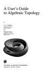
The next diagram (figure 1) was taken from a book of algebraic topology (A User’s
Guide to Algebraic Topology, by Dodson and Parker [2], p. 269) and was produced
by the code:
\newcommand{\sbol}{\small\bfseries}
\begin{xy}
%vertices
(27,0)*+{E^{[0]}=B}="v1";(0,20)*+{E^{[1]}}="v2";(70,20)*+{F^{[1]}}="v3";%
(25,35)*+{K\left(\pi_1(F),1\right)}="v4";%
(95,35)*+{K\left(\pi_1(F),1\right)}="v5";(0,45)*+{\vdots}="v6";%
(70,45)*+{\vdots}="v7";(0,70)*+{E^{[n-1]}}="v8";%
(70,70)*+{F^{[n-1]}}="v9";%
(25,85)*+{K\left(\pi_{n-1}(F),n-1\right)}="v10";%
(95,85)*+{K\left(\pi_{n-1}(F),n-1\right)}="v11";(-20,100)*+{E}="v12";%
(50,100)*+{F}="v13";(0,115)*+{E^{[n]}}="v14";(70,115)*+{F^{[n]}}="v15";%
(25,130)*+{K\left(\pi_{n}(F),n\right)}="v16";%
(95,130)*+{K\left(\pi_{n}(F),n\right)}="v17";
(0,150)*+{\vdots}="v18";(70,150)*+{\vdots}="v19";
%arrows
{\ar@{->>}^{p_{n+1}} "v18"; "v14"};{\ar@{->>} "v19"; "v15"};%
{\ar@{^{(}->} "v16";"v14" };{\ar@{^{(}->} "v17";"v15" };%
21
{\ar@{_{(}->} "v15";"v14" };%
{\ar@{->}^{h_{n}} "v12"; "v14"};{\ar@{->}^{h’_{n}} "v13"; "v15"};%
{\ar@{_{(}->} "v13";"v12" };
{\ar@{->>}^{p_{n}}|(.33){\hole} "v14"; "v8"};%
{\ar@{->}^{h_{n-1}} "v12"; "v8"};{\ar@{->}^{h_{1}} "v12"; "v2"};%
{\ar@{->>} "v15"; "v9"};%
{\ar@{->}^{h’_{n-1}} "v13"; "v9"};{\ar@{->}_{h’_{1}} "v13"; "v3"};%
{\ar@{_{(}->} |(.18){\hole} "v9";"v8" };%
{\ar@{^{(}->} "v10";"v8" };%
{\ar@{^{(}->} "v11";"v9" };
{\ar@{->>} "v8"; "v6"};{\ar@{->>} "v9"; "v7"};%
{\ar@{->>} "v6"; "v2"};{\ar@{->>} "v7"; "v3"};%
{\ar@{^{(}->}|(.35){\hole} "v4";"v2" };%
{\ar@{^{(}->} "v5";"v3" };
{\ar@{->}"v8"; "v1"};%
{\ar@{_{(}->}|(.725){\hole} "v3";"v2" };
{\ar@{->>}_{q_1=p_1}"v2"; "v1"};%
\end{xy}
Finally, here it comes our version of the diagram from Valiente Feruglio ([8],
see also The Latex Graphics Companion [3]). The diagram was produced by the
following code:
\begin{xy}
%vertices
(27,0)*+{E^{[0]}=B}="v1";(0,20)*+{E^{[1]}}="v2";(70,20)*+{F^{[1]}}="v3";%
(25,35)*+{K\left(\pi_1(F),1\right)}="v4";%
(95,35)*+{K\left(\pi_1(F),1\right)}="v5";%
(0,45)*+{\vdots}="v6";(70,45)*+{\vdots}="v7";(0,70)*+{E^{[n-1]}}="v8";%
(70,70)*+{F^{[n-1]}}="v9";(25,85)*+{K\left(\pi_{n-1}(F),n-1\right)}="v10";%
(95,85)*+{K\left(\pi_{n-1}(F),n-1\right)}="v11";(-20,100)*+{E}="v12";%
(50,100)*+{F}="v13";(0,115)*+{E^{[n]}}="v14";(70,115)*+{F^{[n]}}="v15";%
(25,130)*+{K\left(\pi_{n}(F),n\right)}="v16";%
(95,130)*+{K\left(\pi_{n}(F),n\right)}="v17";
(0,150)*+{\vdots}="v18";(70,150)*+{\vdots}="v19";
%arrows
22
..
.
..
.
p n +1
K ( π n ( F ), n )
r Kk
rrr
r
r
rr
r
y rr
[n] o
;E
w
hn www
ww
ww
w
w
E' 4o
'' 44
'' 44
pn
'' 444
'' 44hn−1
K ( π n −1 ( F ), n − 1 )
44
''
k
4
rrr K
''
44
r
r
44
rr
''
yrrr
''
''
E[n−+ 1] o
''
++
++
''
++
''h1
++
''
++
''
++
''
++
'' ..
++
'' .
++
''
++
''
K
++ (rπk 1 ( F ), 1)
''
rK
''
r ++
r
r
+
r
' ++
yrrr
++
E[1] Go G
++
GG
++
GG
++
GG
G
q1 = p1 GGG ++
GG# +
# K ( π n ( F ), n )
r Kk
rrr
r
r
rr
ry rr
? _ [n]
;F
h0n wwww
ww
ww
w
w
? _F
'' 44
'' 44
'' 44
'' 444 h0
44 n−1
''
K ( π n −1 ( F ), n − 1 )
44
k
''
rrr K
44
r
r
''
44
rr
''
yrrr
''
? _ [ n −1]
F
''
''
'
h10 '
''
''
''
''
'' ...
''
''
K ( π1 ( F ), 1)
''
k
''
rrr K
r
r
''
rrr
yrrr
? _ [1]
F
Moore-Postnikov’s tower
of a fibration
E [0] = B
Figure 1: Moore-Postnikov’s tower of a fibration [2]
23
ϕr
L
?Σ

λ L 



i1
LO o
ϕm
i2
O
Lm
o
ΣG
?





Go
/R
O
i4
r
λG
i5
r∗
∗
O
/R
m∗
m∗
m
o G∗
r
ϕm
i6
O
o Kr,m
i3
m
r
o L
r
O
/ R
?Σ



 λ R


/H
/
?Σ
H
λH
{\ar@{->>}^{p_{n+1}} "v18"; "v14"};{\ar@{->>} "v19"; "v15"};%
{\ar@{^{(}->} "v16";"v14" };{\ar@{^{(}->} "v17";"v15" };%
{\ar@{_{(}->} "v15";"v14" };%
{\ar@{->}^{h_{n}} "v12"; "v14"};{\ar@{->}^{h’_{n}} "v13"; "v15"};%
{\ar@{_{(}->} "v13";"v12" };
{\ar@{->>}^{p_{n}}|(.33){\hole} "v14"; "v8"};%
{\ar@{->}^{h_{n-1}} "v12"; "v8"};{\ar@{->}^{h_{1}} "v12"; "v2"};%
{\ar@{->>} "v15"; "v9"};%
{\ar@{->}^{h’_{n-1}} "v13"; "v9"};{\ar@{->}_{h’_{1}} "v13"; "v3"};%
{\ar@{_{(}->} |(.18){\hole} "v9";"v8" };%
{\ar@{^{(}->} "v10";"v8" };%
{\ar@{^{(}->} "v11";"v9" };
{\ar@{->>} "v8"; "v6"};{\ar@{->>} "v9"; "v7"};%
{\ar@{->>} "v6"; "v2"};{\ar@{->>} "v7"; "v3"};%
{\ar@{^{(}->}|(.35){\hole} "v4";"v2" };%
{\ar@{^{(}->} "v5";"v3" };
{\ar@{->}"v8"; "v1"};%
{\ar@{_{(}->}|(.725){\hole} "v3";"v2" };
{\ar@{->>}_{q_1=p_1}"v2"; "v1"};%
\end{xy}
24
References
[1] Campani, C.A.P.: Tutorial de XY-pic (in portuguese), 2006, available from CTAN
[2] Dodson, C.T.J., Parker, P.E.: A User’s Guide to Algebraic Topology, Kluwer Academic Publishers, 1997
[3] Goosens, M., Rahtz, S., Mittelbach, F.: The LATEX Graphics Companion, AddisonWesley, 1997
[4] Rose, K.H.: How to typeset pretty diagram arrows with TEX– design decisions used
in XY-pic, in Jiri Zlatuska, editor, EuroTEX ’92 – Proceedings of the 7th European TEXConference, pages 183-190, Prague, Czechoslovakia, September 1992.
Czechoslovak TEX Users Group.
[5] Rose, K.H.: XY-pic User’s Guide,version 3.7, 1999, available from CTAN
[6] Rose, K.H., Moore, R.: XY-pic Reference Manual, version 3.7, 1999, available
from CTAN
[7] Schubert, H.: Kategorien, vol. I, II, Springer Verlag, 1970
[8] Valiente Feruglio, G.: Typesetting Commutative Diagrams, TUGboat, 15(4), 1994,
466-484.
25