Download ASP modulo CSP: The clingcon system

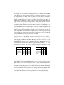
Algorithm 2: FORWARD FILTERING
Input : An inconsistent list of constraints I = [c1 , . . . , cn ].
Output : An irreducible inconsistent list of constraints I 0 .
1
2
3
4
5
6
7
8
9
I 0 ← []
while I 0 is consistent do
T ← I0
i←1
while T is consistent do
T ← T ◦ ci
i←i+1
I 0 ← I 0 ◦ ci
return I 0
hances the information content of the learnt nogood and hopefully speeds up the search
process by better pruning the search space.
In most CP solvers, propagation is done in a constraint space. This space contains
the constraints and the variables of the problem. After doing propagation, the domains
of the variables are restricted. As long as we add further constraints to the constraint
space this effect cannot be undone, as another constraint restricts the domain of the
variables even more. If we want to remove a constraint from a constraint space we have
to create a new space containing only the constraints we want and redo all the propagation. This is why we identified Line 4 in Algorithm 1 as the efficiency bottleneck. To
address this problem, we propose some derivatives of the algorithm.
Forward Filtering is shown in Algorithm 2; it is designed to avoid resetting the search
space of the CP solver. It incrementally adds constraints to a testing list T , starting
from the first assigned constraint to the last one (lines 5 and 6). Remember that incrementally adding constraints is easy for a CP solver as it can only further restrict the
domains. If our test list T becomes inconsistent we add the currently tested constraint
to the result I 0 (lines 5 and 8). If this result is inconsistent (Line 2), we have found a
minimal list of inconsistent constraints. Otherwise, we start again, this time adding all
yet found constraints I 0 to our testing list T (Line 1). Now we have to create a new
constraint space. But by incrementally increasing the testing list, we already reduced
the number of potential candidates that contribute to the IIS, as we never have to check
a constraint behind the last added constraint. We illustrate this again on our example.
We start Algorithm 2 with T = I 0 = [] and
I =[work(lea) = work(adam), work(john) = 0, work(smith) = 0]
◦[work(adam) + work(lea) > 6, work(lea) − work(adam) = 1]
in Line 3. We add work(lea) = work(adam) to T , as this constraint alone is consistent, we loop and add constraints until T = I. As this list is inconsistent, we add the last
constraint work(lea)−work(adam) = 1 to I 0 in Line 8. We can do so, as we know that
the last constraint is indispensable for the inconsistency. As I 0 is consistent we restart