1
Basic 1D and 2D
Experiments
Introduction to 1- and 2dimensional NMR Spectroscopy
Version
001
The information in this manual may be altered without notice.
BRUKER BIOSPIN accepts no responsibility for actions taken
as a result of use of this manual. BRUKER BIOSPIN accepts
no liability for any mistakes contained in the manual, leading to
coincidental damage, whether during installation or operation of
the instrument. Unauthorized reproduction of manual contents,
without written permission from the publishers, or translation
into another language, either in full or in part, is forbidden.
This manual was written and desktop published by
Sandra Loss (Application)
Till Kühn (Application)
© September 2, 2005: Bruker Biospin AG
Fällanden, Switzerland
P/N: xxxxx
DWG-Nr.: 1232001
1
Introduction ___________________________________________________________ 7
1.1
Goals of this course ______________________________________________________ 7
1.2
The NMR Spectrometer __________________________________________________ 8
1.3
Bruker NMR software ____________________________________________________ 8
1.3.1
1.3.2
1.3.3
1.4
Sample Preparation _____________________________________________________ 15
1.5
Tuning and Matching ___________________________________________________ 16
1.5.1
1.5.2
1.5.3
1.6
1.6.1
1.6.2
1.6.3
1.7
1.7.1
1.7.2
2
Tuning and Matching on ATM Probes ____________________________________________ 17
Tuning and Matching 1H (non ATM Probes) _______________________________________ 18
Tuning and Matching 13C (non ATM Probes)_______________________________________ 20
Locking _______________________________________________________________ 21
Autolock ___________________________________________________________________ 21
Adjustment of field and lock phase and power ______________________________________ 21
Optimize lock settings (optional) ________________________________________________ 24
Shimming _____________________________________________________________ 25
Manual Shimming____________________________________________________________ 25
Gradient Shimming ___________________________________________________________ 26
The 1D Proton Experiment ______________________________________________ 27
2.1
2.1.1
2.2
2.2.1
2.2.2
2.3
2.3.1
2.3.2
2.3.3
2.4
2.4.1
2.4.2
3
The basic TopSpin window______________________________________________________ 8
Predefined Parameter Sets______________________________________________________ 10
TopSpin parameters and commands ______________________________________________ 12
General information about the experiment __________________________________ 27
Pulse sequence and a few NMR details____________________________________________ 27
Preparation and Acquisition ______________________________________________ 28
Data acquisition step by step ____________________________________________________ 28
Important acquisition parameters for this experiment _________________________________ 29
Spectral processing _____________________________________________________ 30
Automatic processing _________________________________________________________ 30
Manual processing ___________________________________________________________ 30
Processing parameters _________________________________________________________ 33
Post-processing_________________________________________________________ 34
Peak picking ________________________________________________________________ 34
Integration __________________________________________________________________ 35
2.5
Spectra interpretation ___________________________________________________ 37
2.6
Possible pitfalls _________________________________________________________ 40
Basic 13C Experiments __________________________________________________ 44
3.1
3.1.1
3.2
3.2.1
3.2.2
3.3
3.3.1
3.3.2
3.3.3
3.4
3.4.1
3.4.2
General information about the experiments _________________________________ 44
Pulse sequences and a few NMR details ___________________________________________ 44
Preparation and Acquisition ______________________________________________ 47
Data acquisition step by step ____________________________________________________ 47
Important acquisition parameters for this experiment _________________________________ 48
Spectral processing _____________________________________________________ 49
Automatic processing _________________________________________________________ 49
Manual processing ___________________________________________________________ 49
Processing parameters _________________________________________________________ 52
Post-processing_________________________________________________________ 52
Peak picking ________________________________________________________________ 53
Integration __________________________________________________________________ 54
Avance 1D/2D
Bruker
3
4
3.5
Spectra interpretation ___________________________________________________ 56
3.6
Possible pitfalls _________________________________________________________ 58
13
C Experiments to Assess Multiplicities: DEPT and APT______________________ 60
4.1
General information about the experiments _________________________________ 60
4.1.1
4.2
Pulse sequences and a few NMR details ___________________________________________ 60
Preparation and Acquisition ______________________________________________ 62
4.2.1
4.2.2
4.3
Data acquisition step by step ____________________________________________________ 62
Important acquisition parameters for these experiments _______________________________ 64
Spectral processing _____________________________________________________ 65
4.3.1
4.3.2
4.3.3
4.4
Automatic processing _________________________________________________________ 65
Manual processing ___________________________________________________________ 65
Processing parameters _________________________________________________________ 68
Post-processing_________________________________________________________ 69
4.4.1
5
Peak picking ________________________________________________________________ 69
4.5
Spectra interpretation ___________________________________________________ 70
4.6
Possible pitfalls _________________________________________________________ 71
The COSY Experiment__________________________________________________ 73
5.1
General information about the experiment __________________________________ 73
5.1.1
5.2
Pulse sequence and a few NMR details____________________________________________ 73
Preparation and Acquisition ______________________________________________ 75
5.2.1
5.2.2
5.3
Data acquisition step by step ____________________________________________________ 75
Important acquisition parameters for this experiment _________________________________ 76
Spectral processing _____________________________________________________ 80
5.3.1
5.3.2
5.3.3
5.3.4
5.4
Automatic processing _________________________________________________________
Manual processing ___________________________________________________________
Processing parameters _________________________________________________________
Processing parameters _________________________________________________________
Post-processing_________________________________________________________ 88
5.4.1
5.4.2
6
80
80
82
86
Peak picking ________________________________________________________________ 88
Projections__________________________________________________________________ 89
5.5
Spectra interpretation ___________________________________________________ 90
5.6
Possible pitfalls _________________________________________________________ 92
The TOCSY Experiment ________________________________________________ 96
6.1
General information about the experiment __________________________________ 96
6.1.1
6.2
Pulse sequence and a few NMR details____________________________________________ 96
Preparation and Acquisition ______________________________________________ 97
6.2.1
6.2.2
6.3
Data acquisition step by step ____________________________________________________ 97
Important acquisition parameters for this experiment _________________________________ 98
Spectral processing ____________________________________________________ 100
6.3.1
6.3.2
6.3.3
6.4
Automatic processing ________________________________________________________ 100
Manual processing __________________________________________________________ 101
Processing parameters ________________________________________________________ 103
Post-processing________________________________________________________ 105
6.4.1
6.4.2
Peak picking _______________________________________________________________ 105
Projections_________________________________________________________________ 106
6.5
Spectra interpretation __________________________________________________ 107
6.6
Possible pitfalls ________________________________________________________ 108
4
Bruker
Avance 1D/2D
7
The NOESY Experiment _______________________________________________ 111
7.1
General information about the experiment _________________________________ 111
7.1.1
7.2
Preparation and Acquisition _____________________________________________ 112
7.2.1
7.2.2
7.2.3
7.3
7.4
Peak picking _______________________________________________________________ 122
Projections_________________________________________________________________ 123
7.5
Spectra interpretation __________________________________________________ 124
7.6
Possible pitfalls ________________________________________________________ 125
The ROESY Experiment _______________________________________________ 127
8.1
General information about the experiment _________________________________ 127
8.1.1
8.2
Pulse sequence and a few NMR details___________________________________________ 127
Preparation and Acquisition _____________________________________________ 128
8.2.1
8.2.2
8.2.3
8.3
Data acquisition step by step ___________________________________________________ 128
Important acquisition parameters for this experiment ________________________________ 129
Optimization of the mixing time ________________________________________________ 131
Spectral processing ____________________________________________________ 133
8.3.1
8.3.2
8.3.3
8.4
Automatic processing ________________________________________________________ 133
Manual processing __________________________________________________________ 133
Processing parameters ________________________________________________________ 136
Post-processing________________________________________________________ 138
8.4.1
8.4.2
Peak picking _______________________________________________________________ 138
Projections_________________________________________________________________ 139
8.5
Spectra interpretation __________________________________________________ 139
8.6
Possible pitfalls ________________________________________________________ 141
The HMQC Experiment________________________________________________ 142
9.1
General information about the experiment _________________________________ 142
9.1.1
9.2
Pulse sequence and a few NMR details___________________________________________ 142
Preparation and Acquisition _____________________________________________ 143
9.2.1
9.2.2
9.3
Data acquisition step by step ___________________________________________________ 144
Important acquisition parameters for this experiment ________________________________ 145
Spectral processing ____________________________________________________ 148
9.3.1
9.3.2
9.3.3
9.4
Automatic processing ________________________________________________________ 148
Manual processing __________________________________________________________ 149
Processing parameters ________________________________________________________ 151
Post-processing________________________________________________________ 153
9.4.1
9.4.2
10
Automatic processing ________________________________________________________ 117
Manual processing __________________________________________________________ 117
Processing parameters ________________________________________________________ 120
Post-processing________________________________________________________ 122
7.4.1
7.4.2
9
Data acquisition step by step ___________________________________________________ 112
Important acquisition parameters for this experiment ________________________________ 113
Optimization of the mixing time ________________________________________________ 116
Spectral processing ____________________________________________________ 117
7.3.1
7.3.2
7.3.3
8
Pulse sequence and a few NMR details___________________________________________ 111
Peak picking _______________________________________________________________ 153
Projections_________________________________________________________________ 154
9.5
Spectra interpretation __________________________________________________ 154
9.6
Possible pitfalls ________________________________________________________ 155
The HMBC Experiment ______________________________________________ 157
Avance 1D/2D
Bruker
5
10.1
General information about the experiment _________________________________ 157
10.1.1
10.2
Preparation and Acquisition _____________________________________________ 158
10.2.1
10.2.2
10.3
Data acquisition step by step ________________________________________________ 158
Important acquisition parameters for this experiment _____________________________ 159
Spectral processing ____________________________________________________ 162
10.3.1
10.3.2
10.3.3
10.4
Pulse sequence and a few NMR details ________________________________________ 157
Automatic processing ______________________________________________________ 162
Manual processing ________________________________________________________ 163
Processing parameters _____________________________________________________ 164
Post-processing________________________________________________________ 166
10.4.1
10.4.2
Peak picking _____________________________________________________________ 166
Projections ______________________________________________________________ 167
10.5
Spectra interpretation __________________________________________________ 167
10.6
Possible pitfalls ________________________________________________________ 167
11
The HSQC Experiment ______________________________________________ 169
11.1
General information about the experiment _________________________________ 169
11.1.1
11.2
Preparation and Acquisition _____________________________________________ 170
11.2.1
11.2.2
11.3
Data acquisition step by step ________________________________________________ 170
Important acquisition parameters for this experiment _____________________________ 172
Spectral processing ____________________________________________________ 175
11.3.1
11.3.2
11.3.3
11.4
Pulse sequence and a few NMR details ________________________________________ 169
Automatic processing ______________________________________________________ 176
Manual processing ________________________________________________________ 176
Processing parameters _____________________________________________________ 178
Post-processing________________________________________________________ 180
11.4.1
11.4.2
Peak picking _____________________________________________________________ 180
Projections ______________________________________________________________ 181
11.5
Spectra interpretation __________________________________________________ 182
11.6
Possible pitfalls ________________________________________________________ 182
12
Plotting ___________________________________________________________ 184
12.1
Starting the program ___________________________________________________ 184
12.2
Plotting a 1D spectrum _________________________________________________ 185
12.2.1
12.2.2
12.3
Basic editing of a 1D spectrum_______________________________________________ 185
Inserting an expansion _____________________________________________________ 187
Plotting of a 2D spectrum _______________________________________________ 187
12.3.1
6
Basic editing of a 2D spectrum_______________________________________________ 188
Bruker
Avance 1D/2D
1 Introduction
1.1 Goals of this course
The goal of the present course is to give you an introduction into the basic
one- and two dimensional experiments that are commonly used to solve
structural problems.
We will start with an overview over sample preparation and the basic
spectrometer setup and handling. On the experimental side we will cover
proton and heteronuclear 1D experiments, as well as homonuclear and
inverse 2D experiments. The description of the experiments covers the basic
principle, the information content and interpretation of the spectra, as well as
the setup of the acquisition and processing parameters. An individual chapter
covers the plotting of 1D and 2D spectra.
This manual refers to the use of the TopSpin software. Compared to the
former software XWIN-NMR it offers many intuitive buttons and interactive
possibilities which are described throughout this manual. However, for all of
these tasks there is also a command existing that can be typed onto the
command line or can be chosen from the menu and will then have exactly the
same effect. For not confusing customers, who still work with XWIN-NMR
these commands are still given.
We hope that we will have convinced you by the end of the course, that NMR
is not a mysterious world that can only be understood by some specialised
scientists, but a very powerful tool that can easily help you in structural
questions.
The application team of Bruker Switzerland.
Avance 1D/2D
Bruker
7
1.2 The NMR Spectrometer
The NMR spectrometer consists of three major components: (1) The
superconducting magnet with the probe, which contains the sample to be
measured; (2) The console, which contains all the electronics used for
transmission and reception of radio frequency (rf) pulses through the preamplifier to the probe; (3) The computer, from where the operator runs the
experiments and processes the acquired NMR data.
1.3 Bruker NMR software
There are three major tasks that are controlled by the NMR software:
acquisition, processing and plotting. The TopSpin program is the user
interface for all of these tasks. Compared to the former XWIN-NMR software,
TopSpin is much more intuitive for people who had been working with other
windows programs before. However, all the basic commands you were used
to from XWIN-NMR will still work on TopSpin!
1.3.1 The basic TopSpin window
The basic TopSpin window is displayed in Figure 1.1
Like before, the commands can be called up by selecting the items from the
menu bar (1, Figure 1.1) or by typing the appropriate command in the
command line (2, Figure 1.1). Additionally there is an icon bar (3, Figure 1.1)
that contains some buttons which will execute some more often used
commands. This bar can be customized by the user, i.e. buttons can be
added or deleted with respect to your own needs!
The main window always contains the active screen. This possesses an
extra menu bar (4, Figure 1.1) where you can choose, what you actually
would like to be displayed in the main window. If you are setting up an
experiment, you will have access to the acquisition and processing
parameters, to the FID, the spectrum, title, pulse program and so on.
Whenever you click on one of these tacks, the respective parameters or
figures will be displayed and can eventually be altered.
These parameters and the measured data as well as the processed spectra
are stored in specific datasets. The file tree has the following general
structure:
Bruker/TopSpin/data/user_name/nmr/exp_name/exp_no/pdata/proc_no
Under this path, the files can be found on your computer. In TopSpin you
can get a reduced file tree (the parts of the tree that are always kept the
same are omitted) projected in your window (5, Figure 1.1) if you click on the
arrow cursor on the left edge (6, Figure 1.1) to open up a side window and
chose the Browser from the tags. If the directory where the data is stored is
not directly displayed it can be included with a right mouse click on the
window. Choose the option “Add New Data Dir …” and type in the path,
where your NMR data can be found. After clicking “OK” the directory will be
8
Bruker
Avance 1D/2D
added to the file tree. To open an existing data set simply click on the
desired experiment file with the left mouse button and drag it into the main
display window.
Figure 1.1: The TopSpin window
1
2
7
6
4
5
8
3
Note, that it is now possible to have several spectral windows open at the
same time! Every open window is represented by a small colored and
numbered square (7, Figure 1.1). Clicking on one of these will bring you back
to the according window.
By clicking on the grey field below the command line with the right mouse
button, the acquisition status bar (8, Figure 1.1) can be switched on and off.
This bar yields some information about the actual status of the system:
whether it is pulsing or not, how many scans and/or increments had been
running already, the actual lock level, and so on.
To alter the display properties of the basic TopSpin window, type setres on
the command line. A dialog box will open that allows you to choose colors,
start up options, layout, etc.
If more or less information is needed on the spectral display window, right
click with the mouse inside that window. A small dialog box will open that
Avance 1D/2D
Bruker
9
allows you to choose, whether the cursor information, peak labels, title,
integrals, etc. should be displayed in this window.
Whenever any icon is clicked or a command is given that needs some
interactive input from the user (for example manual phase correction,
baseline correction or integration) the main display window will switch to a
display that is appropriate for the desired task. While the spectrum is still
displayed, the menu tags on top are replaced by some icons that allow an
easy access to all important parameters for the task (see Figure 1.2).
Figure 1.2: Icon bar in the phase correction mode.
1.3.2 Predefined Parameter Sets
To record spectra, a lot of parameters need to be adjusted in order to get
reliable results. To make this task a little easier the basic philosophy is to
work with predefined parameter sets that are already included in the software
and exist for a whole range of different spectroscopic experiments. These
parameter sets include the pulse program, acquisition and processing AU
programs as well as all other necessary parameters except spectrometer
specific values for pulse lengths and power levels. With a few exceptions, the
standard parameter sets have the same base name as the corresponding
pulse program. Each parameter set can be read into a dataset of your choice
by the command rpar. You can modify the parameters and save the new
parameter set by the command wpar. Bruker predefined parameter sets are
written in capital letters, and we recommend that you do not change them but
rather create new ones that you can use just as well.
The following list is a short summary of the most commonly used
experiments and the corresponding parameter sets. The emphasis is on the
spectroscopic information that you will get from the experiments rather than
on the type of experiment. (For the experiments in this table, it is always
recommended to use the gradient version of the experiment if you have the
required z-gradient hardware. These experiments usually require less time
than the ones without gradients).
10
Bruker
Avance 1D/2D
Table 1.1: Short List of Typical Experiments, Parameter Sets and What They Do
Atom / Group
H
Information (1D Experiments)
1
H chemical shift and coupling
C
13
C
C
CH, CH2, CH3
CH
CH,CH2, CH3
C
a.k.a.
1D1H
C chemical shift, 1H decoupled (signal 1D13C
enhancement, integration not possible)
13
C chemical shift, 1H coupled (signal
1D13C
enhancement, integration not possible)
13
C chemical shift, 1H decoupled (no
1D13C
signal enhancement, integration possible)
13
C chemical shift, select CH, CH2 and
DEPT45
CH3 signals only (same phase)
13
C chemical shift, select CH signals only DEPT90
13
C chemical shift, select CH, CH3 and
DEPT135
CH2 signals only (opposite phase)
13
C chemical shift, C and CH2 have the APT
opposite phase from CH and CH3
Parameter Set
PROTON
C13CPD
C13GD
C13IG
C13DEPT45
C13DEPT90
C13DEPT135
C13APT
Correlation Information (2D Experiments)
a.k.a.
1
H–H
H/1H nearest neighbor, through bond chemicalCOSY
shift correlation
1
H–H
H/1H nearest neighbor, through bond chemicalDQFshift correlation plus coupling constants
COSY
1
H–(–)nH
H/1H total spin system through bond chemicalTOCSY
shift correlation
C–H
Sensitive 1H/13C directly bound chemical shiftHSQC
correlation (one bond), lower resolution in 13CHMQC
dimension
C–H
Sensitive 1H/13C directly bound chemical shiftBIRDcorrelation (one bond), lower resolution in 13CHMQC
dimension (small molecules, solemnly select
13
C/1H not 12C/1H)
C–(–)nH
Sensitive 1H/13C long range chemical shiftHMBC
correlation (more than one bond), lower
resolution in 13C dimension
1
…
H/1H non bound structural neighbor, throughROESY
H H
space chemical shift correlation (small molecules,
low fields)
1
…
H/1H non bound structural neighbor, throughNOESY
H H
space chemical shift correlation (large molecules,
proteins)
Parameter Set
COSYGPSW1
COSY45SW
COSYGPDFPHSW1
COSYDQFPHSW
MLEVPHSW
HSQCGP1
HMQCPH
HMQCBIPH
HMBCLPND
ROESYPH
NOESYPH
In most of the 2D parameter sets there is a spectral width optimization
implemented. So if you acquire the corresponding 1D experiments in the
previous experiment number the spectral width for the 2D will be optimized
according to the 1D information.
A complete list of parameter sets can be called up by typing rpar without a
following name. The nomenclature of the parameter sets follows the rules for
the nomenclature of the pulse programs. They can be found in the file:
$TopSpinHome/exp/stan/nmr/lists/pp/Pulprog.info
1
z-gradient hardware required
Avance 1D/2D
Bruker
11
1.3.3 TopSpin parameters and commands
A list of commonly used acquisition and processing commands and
parameter names as well as a description of the corresponding command or
parameter is given in short in the tables below.
Table 1.2: General Commands and AU Programs
setres
edmac
edau
edpul
xau listall_au
edcpul
customize the TopSpin interface
edit or create a TopSpin macro
edit or create a TopSpin AU program
edit or create a TopSpin pulse program
create a file called “listall” in your home directory with a list of all
available AU programs including short descriptions
edit the current pulse program
Table 1.3: Data Set Related Commands
edc, new
xau iexpno
wrpa
re
rep
browse
search
wpar
rpar
create a new data set, experiment number or processing number
copy the current experiment number including all parameters to the
consecutive experiment number
copy of the current data set including the spectra
move to a specific experiment number within the data set
move to a processing number within the experiment number
browse the data set directories
find a specific data set
save the current parameters
select and read a predefined parameter set
Table 1.4: Acquisition Parameters
ns
ds
td
sw
aq
o1p
o2p
rg
pulprog
aunmp
number of scans
number of dummy scans
Time domain, number of acquired data points
sweep width in ppm
acquisition time
transmitter frequency of f1 channel in ppm
transmitter frequency of f2 channel in ppm
receiver gain
definition of the pulse program
definition of the acquisition AU program
Table 1.5: Acquisition and Pre-acquisition Commands
edhead
edprosol
getprosol
xau pulse
edasp
edcpul
eda
ased
spdisp
dpa
wbchan
12
define the current probehead
define probehead specific pulse lengths and power levels (3.0)
use probehead specific pulse lengths and power levels in the
current pulse program (3.0)
calculate the power level from pulse lengths and vice versa
configure the routing of the spectrometer
open the current pulse program in a text editor window
edit all acquisition parameters
edit the acquisition parameters that are relevant for the current
pulse program
open the graphical pulse program editor (3.0)
display all status parameters for the acquisition
select the wobbling channel for tuning and matching
Bruker
Avance 1D/2D
wobb
atma
atmm
edsolv
edlock
lock
lockdisp
rsh
gradshim
wsh
edte
edau
stdisp
expt
rga
zg
xaua
gs
tr
halt, stop
kill
tuning and matching the probe
automatic tune and match the ATM probe
manually tune and match the ATM probe
define solvent parameters
define lock parameters for probhead and solvent
automatically lock on solvent (parameters defined in edlock)
open the lock display window
select and read shim values
start the gradient shimming subprogram
save the current shim values
open the temperature control window
select or edit AU programs
open the shape tool
estimate the experiment time
automatically adjust the receiver gain
start acquisition
start the acquisition AU program (this also starts the acquisition)
interactive adjustment of acquisition parameters
data transfer during acquisition
stop the acquisition
kill a specific process
Table 1.6: Processing Parameters
si
phc0, phc1
lb
aunmp
size of the real spectrum
parameters for zero order and first order phase corrections
line broadening factor for em
definition of the processing AU program
Table 1.7: Processing Commands
edp
dpp
ft
em
ef
phase
apk
abs
efp
sr
sref
edc2
dual
edo
edg
view
plot
edit all processing parameters
display all status parameters for processing
Fourier transform the current data
apply exponential window function
combined command of ft and em
set the phase correction defined by phc0 and phc1
automatically phase correct the spectrum
automatically baseline correct and integrate the spectrum
combined command of ft, em and phase
spectral referencing
automatically calibrate the spectrum
select a second and a third data processing number
invoke the dual display
select an output device
edit all graphics and plotting parameters
plot preview
start the plot program
Table 1.8: Pulse Program Specific Parameters
pl1
pl2
pl9
pl10
pl11
pl12
Avance 1D/2D
f1 channel - power level for pulse (default)
f2 channel - power level for pulse (default)
f1 channel - power level for presaturation
f1 channel - power level for TOCSY-spinlock
f1 channel - power level for ROESY-spinlock
f2 channel - power level for CPD/BB decoupling
Bruker
13
pl14
pl15
f2 channel - power level for cw saturation
f2 channel - power level for TOCSY-spinlock
sp1
f1 channel - shaped pulse for selective excitation or f1 channel shaped pulse for water flipback
f1 channel - shaped pulse 180 degree or f2 channel - shaped pulse
90 degree (on resonance)
f2 channel - shaped pulse 180 degree (off resonance2) or f2
channel - shaped pulse 180 degree (adiabatic) or f1 channel shaped pulse for wet
sp2
sp7
p15
p16
p17
p18
for different applications i.e. f1 channel - variable flip angle high power
pulse in DEPT
f1 channel - 90 degree high power pulse
f1 channel - 180 degree high power pulse
f2 channel - 90 degree high power pulse
f2 channel - 180 degree high power pulse
f1 channel - 90 degree low power pulse
f1 channel - 90 degree shaped pulse (selective excitation or water
flipback/watergate or wet)
f1 channel - pulse for ROESY spinlock
homospoil/gradient pulse
f1 channel - trim pulse at pl10 or pl15
f1 channel - shaped pulse (off resonance presaturation)
d0
d1
d2
d3
d4
d6
d7
d8
d9
d11
d12
d14
d16
d17
d18
d19
d20
incremented delay (2D)
[3 usec]
relaxation delay 1-5 * T1
1/(2J)
1/(3J)
1/(4J)
delay for evolution of long range couplings
delay for inversion recovery
NOESY mixing time
TOCSY mixing time
delay for disk I/O
[30 msec]
delay for power switching
[20 usec]
delay for evolution after shaped pulse
delay for homospoil/gradient recovery
delay for DANTE pulse-train
delay for evolution of long range couplings
delay for binomial water suppression
for different applications
cnst0
cnst1
cnst2
cnst3
cnst4
cnst5
cnst11
cnst12
for different applications
J (HH)
J (XH)
J (XX)
J (YH)
J (XY)
for multiplicity selection
for multiplicity selection
vc
vd
variable loop counter, taken from vc-list
variable delay, taken from vd-list
l1
l2
l3
loop for MLEV cycle (((p6*64) + p5) * l1) + (p17*2) = mixing time
loop for GARP cycle l2 * 31.75 * 4 * p9 => AQ
loop for phase sensitive 2D or 3D using States et al. or States-TPPI
method l3 = td1/2
for different applications i.e. noediff
p0
p1
p2
p3
p4
p6
p11
l4
14
Bruker
Avance 1D/2D
Note that the default units for pulses are microseconds (u), the units for
delays are seconds (s), but one can always enter a value combined with a
unit to define a time slot in TopSpin. The nomenclature here is: s = seconds,
m = milliseconds and u = microseconds. For example to set the value of d1
to 500m would define d1 to last for half a second.
The complete information on the nomenclature and default usage of the
pulse program parameters can be found in:
$TopSpinHome/exp/stan/nmr/lists/pp/Param.info
The nomenclature and description of the standard pulse programs and
predefined parameter sets can be found in:
$TopSpinHome/exp/stan/nmr/lists/pp/Pulprog.info
Acquisition, processing and plotting commands can be given either in the
TopSpin command line or via menu selection. Examples are zg, which starts
the acquisition, ft which performs a Fourier transformation on the current
data or apk which invokes the automatic phase correction.
Another possibility to manage different task in TopSpin are AU programs.
They handle many routine jobs and can be selected or edited by the edau
command. AU programs have to be compiled before first usage. Compile and
start AU Programs by entering xau followed by the program name.
TopSpin also offers extensive online documentation, which can be accessed
via the help menu in the TopSpin menu bar.
1.4 Sample Preparation
An accurate sample preparation can prevent many nuisances, therefore you
should pay maximum attention on this. The following points should be
considered:
•
Use only clean and dry sample tubes to prevent contamination.
Scratches or poor quality tubes may result in difficulties with shimming.
•
The solvent must be deuterated to prevent intense proton signals and
for locking. If you need to observe OH- or NH-protons, the solvent
should be free of exchangeable protons. In cases where you need to
run such spectra in a solvent with exchangeable protons, you can use a
mixture of 5-10% deuterated and 90-95 % non-deuterated solvents.
•
The amount of the compound you should use depends on the size of
the molecule and the type of experiment you want to run. For a
medium-sized organic molecule an amount of ½ - 1 mg is fully
sufficient for a 1D proton experiment, whereas you should better use 2
– 5 mg if you also want to run direct observe carbon spectra.
Avance 1D/2D
Bruker
15
•
The optimum filling height of the sample tube is 4 cm, corresponding
to about 0.6 ml solvent for 5 mm and 4 ml for 10 mm tubes. Using to
little solvent results in shimming problems. You can minimize necessary
shimming between different samples, if you always use the same filling
height.
•
The solution should be clear and homogenous. Precipitations should
be filtered off, concentration gradients should be prevented by shaking
the tube after adding additional solvent or compound.
•
Adjust the sample tube in the spinner using the sample gauge as a
meter. For most probes, the appropriate sample depth is about 2 cm
(the sample depth is noted in the binder coming with the probe). If you
use less than 4 cm filling height, you should adjust the sample in a way
that the solution is centred around the 0-line of the sample gauge.
•
Make sure, that the tube is held tightly by the spinner, for high or deep
temperature experiments use the ceramic spinner. If you are running
experiments with spinning, make sure, that the reflectors on the spinner
are clean. This is important for maintaining the correct spinning rate.
•
Wipe the sample tube clean before inserting it into the magnet.
•
Turn on the lift with the “Lift” button on the BSMS panel or by typing ej
on the command line. Place the sample with the spinner on the air
cushion and press the “Lift” button again or type ij, respectively, to
insert the sample.
1.5 Tuning and Matching
In a probehead there are resonant circuits for each nucleus indicated on the
probehead label (e.g., one for 1H and one for 13C in a dual 1H/13C probehead;
one for 1H and one for a wide range of nuclei in BBO or BBI probeheads).
There is also a resonant circuit for the lock nucleus, but the standard user will
never need to adjust this, so we will ignore it in the following section. Each of
the circuits has a frequency at which it is most sensitive (the resonance
frequency). Once the sample is inserted, the probehead should be tuned and
matched for these individual frequencies.
Tuning is the process of adjusting this frequency until it coincides with the
frequency of the pulses transmitted to the circuit. For example, the frequency
at which the 1H resonant circuit is most sensitive must be set to the carrier
frequency of the 1H pulses (which is sfo1 if the 1H circuit is connected to the
f1 channel, sfo2 if it is connected to the f2 channel, etc.). Matching is the
process of adjusting the impedance of the resonant circuit until it corresponds
with the impedance of the transmission line connected to it. This impedance
is 50 Ω. Correct matching maximizes the power that is transmitted to the coil.
A probehead is said to be tuned and matched when all of its resonant circuits
are tuned and matched. Once a probehead has been tuned and matched, it
is not necessary to retune or rematch it after slight adjustments of the carrier
frequency, since the probehead is generally tuned and matched over a range
of a couple of hundred kHz. On the other hand, large adjustments to the
carrier frequency, necessary when changing nuclei, warrant retuning and
rematching of the probehead. Thus, a broadband probe needs to be retuned
Bruker
Avance 1D/2D
16
and rematched each time the heteronucleus is changed. Also a change of
the solvent shows some effect on the tuning and matching, so you should
always perform these actions with the sample tube inserted in the magnet
and eventually retune and match after a solvent change. This is especially
important for the proton channel as the solvents influence is larger for higher
resonance frequencies than for the lower ones.
1.5.1 Tuning and Matching on ATM Probes
If you have an ATM probe, enter edasp or press the button
in the
AcquPars menu of the main window and set the spectrometer parameters for
the channels that should be matched and tuned. For 1H on channel F1 and
13C on channel F2 enter the following values (Figure 1.3):
NUC1
NUC2
NUC3
1H
13C
OFF
This automatically sets sfo1 to a frequency appropriate for 1H and sfo2 to
the corresponding 13C frequency for tuning and matching. Exit edasp by
clicking
.
Type atma. This will invoke the automatic tune and match program for all
nuclei that were selected previously in edasp. Therefore it is not necessary
to tune and match manually.
Figure 1.3: The channel selection window.
Avance 1D/2D
Bruker
17
1.5.2 Tuning and Matching 1H (non ATM Probes)
If the NMR experiments to be performed are 1H homonuclear experiments
(e.g., 1H 1D spectroscopy, COSY, NOESY, or TOCSY), only the 1H circuit of
the probehead has to be tuned and matched.
Make sure that the sample is in the magnet, and the probehead is connected
for standard 1H acquisition. Note that there is no special configuration for
tuning and matching. It is recommended to tune and match without sample
spinning.
Set the Parameters
Enter edasp or press the button
in the AcquPars menu of the main
window and set the following spectrometer parameters:
NUC11H
NUC2OFF
NUC3OFF .
This automatically sets sfo1 to a frequency appropriate for 1H tuning and
matching. There is no need to adjust sfo1 carefully now. Exit edasp by
clicking
.
Start Wobbling
Tuning and matching are carried out simultaneously. During wobbling, a low
power signal is transmitted to the probehead. This signal is swept over a
frequency range determined by the parameter wbsw (the default value is
4 MHz) centered around the carrier frequency (i.e., sfo1, sfo2, etc.,
depending on which nucleus is being tuned/matched). Within the preamplifier
(High Performance Preamplifier Assembly or HPPR), the impedance of the
probe over this frequency range is compared to the impedance of a 50 Ω
resistor. The results are shown both on the LED display of the HPPR and in
the acquisition submenu of TopSpin. Both displays show the reflected power
of the probehead versus the frequency of the signal. The user observes
either one or both of these displays while tuning and matching the
probehead.
Before starting the wobbling procedure, ensure that no acquisition is in
progress, e.g., enter stop.
Enter acqu to switch to the acquisition window of TopSpin, if it is desired to
use this to monitor the tuning and matching.
Start the frequency sweep by typing wobb. The curve that appears in the
acquisition window is the reflected power as a function of frequency. Unless
the probehead is quite far from the correct tuning and matching, there will be
a noticeable dip in the curve. When the 1H circuit is properly tuned, the dip
will be in the center of the window, denoted by the vertical marker; and when
the circuit is properly matched, the dip will extend all the way down to the x
axis (Figure 1.4). Similar information is conveyed by the LED display on the
HPPR. The horizontal row of LED's indicates tuning and the vertical row
matching. When the circuit is properly tuned and matched, the number of
LEDs is minimized. This usually means that only green LED’s are lit in both
the horizontal and vertical displays.
18
Bruker
Avance 1D/2D
Figure 1.4: Wobbling curve as shown in the acquisition window.
Tune and Match
Adjust the tuning and matching screws (labeled T and M) at the base of the
probehead. The screws are having the same color as the nucleus on the
front panel of the probehead and those for the 1H circuit are usually yellow.
Note that the screws have a limited range and attempting to turn them
beyond this range will damage the probehead.
Since there is an dependence between tuning and matching, it is generally
useful to adjust the T and M screws in an iterative fashion. Turn the M screw
until the dip is well matched at some frequency (the dip extends to the x axis
and the number of LED’s lit in the vertical HPPR display is minimized). Most
likely this will not be the desired frequency. Adjust the T screw slightly to
move the dip towards the center of the window, or equivalently, to reduce the
number of LED’s lit in the horizontal HPPR display. Rematch the dip by
adjusting the M screw again. Note that it is possible to run out of range on the
M screw. If this happens, return M to the middle of its range, adjust T to get a
well matched dip at some frequency, and walk the dip towards the correct
frequency as described above.
As mentioned above, ideal tuning and matching is when the dip is centered in
the window and extends to y = 0 (the x axis) on the acquisition window
(Figure 1.4), or equivalently, when the number of LED's lit on the preamplifier
is minimized in both the vertical and horizontal display.
Avance 1D/2D
Bruker
19
When the 1H circuit is tuned and matched, exit the wobble routine by typing
stop or pressing the button
. Click on
to exit the acquisition window
and return to the main window.
1.5.3 Tuning and Matching 13C (non ATM Probes)
Since most 13C experiments make use of 1H decoupling, besides 13C the 1H
should be tuned and matched as well. When tuning and matching a
probehead with multiple resonant circuits, it is best to tune and match the
lowest frequency circuit first. Thus, when tuning and matching a probehead
for both 1H and 13C, first do the 13C and then the 1H adjustments. However, if
you proceed with the procedure as described below, TopSpin will take care
of this by showing the lowest frequency wobbling curve first and going then to
the higher frequencies whenever you change the channel.
Make sure that the sample is in the magnet, and the probehead is connected
for the appropriate experiment. It is recommended to tune and match without
sample spinning.
Set the Parameters
Enter edasp or press the button
in the AcquPars menu of the main
window and set the following spectrometer parameters:
NUC113C
NUC2 1H
NUC3OFF .
This automatically sets sfo1 and sfo2 to a frequency appropriate for
1
H tuning and matching. Exit edasp by clicking
.
13
C and
Start Wobbling, Tune and Match
Ensure that no acquisition is in progress, enter stop.
Enter acqu to switch to the acquisition window, if this will be used to monitor
the tuning and matching.
Start the frequency sweep by typing wobb. The curve that appears in the
acquisition window is for 13C. Adjust the tuning and matching following the
guidelines given above for 1H. Note that some probeheads (e.g., broadband
probeheads) have sliding bars instead of screws, one set labeled tuning and
another labeled matching. Set the tuning and matching sliding bars to the
values indicated for 13C on the menu. Adjust the tuning and matching bars
until the dip is well tuned and matched at some frequency as described
above for 1H.
Now the channel can be switched to the 1H channel by clicking the channel
select button
. Adjust the tuning and matching for the protons with the
screws while monitoring it via the LED’s on the HPPR or the display on the
computer.
Once the probehead is tuned and matched for 13C and 1H, exit the wobble
routine by typing stop or pressing the button
. Click on
to exit the
acquisition window and return to the main window.
20
Bruker
Avance 1D/2D
1.6 Locking
Before running an NMR experiment, it is necessary to lock and shim the
magnetic field.
In the acquisition status bar, there is a small icon, displaying either the lock
level or giving a number, which belongs to the height of the lock level in
percent. The desired display can be toggled in the user preference dialog
window that can be started with the command setres. To get a bigger display
in the main window you can either press the button
in the menu bar or
enter lockdisp on the command line. This opens a window in which the lock
trace appears. You can detach this window from the main TopSpin window
by clicking the button
in the menu bar of the lock window.
1.6.1 Autolock
The most convenient way to lock is to use the TopSpin command lock. To
start the lock-in procedure, enter lock and select the appropriate solvent from
the list. Alternatively, enter the solvent name together with the lock
command, e.g., lock cdcl3. During lock-in, several parameters such as the
lock power, the field value, and the frequency shift for the solvent are set
according to the values in the lock table. This table can be edited using the
command edlock. Note that the lock power listed in this table is the level
used once lock-in has been achieved. The field-shift mode is then selected
and autolock is activated. Once lock-in is achieved, the lock gain is
automatically adjusted to a value that the lock signal is visible in the lock
window. At this point the message “lock: finished” appears in the status line
at the bottom of the window.
The lock-in procedure outlined above sets the frequency shift to the exact
frequency shift value for the given solvent as listed in the edlock table. It also
sets the field value to the value listed in the edlock table and then adjusts it
slightly to achieve lock-in (the absolute frequency corresponding to a given
ppm value no longer depends on the lock solvent). Following this lock-in
procedure, the solvent parameter in the eda table is set automatically, which
is important if you wish to use the automatic calibration command sref (see
chapter 2.3.2).
1.6.2 Adjustment of field and lock phase and power
If the lock settings have not been adjusted for a long time or when changing
the probehead it is possible that some problems during the locking procedure
occur. This is mostly due to inappropriate values for the magnetic field or the
lock phase. To check these values, it is best to monitor the sweep wiggles
that will be displayed, if the sample is not locked, but the magnetic field is
swept. If the lock phase and the field are set correctly, the signal is centered
with both inner wiggles pointing up and without any phase distorsion (Figure
1.5).
Figure 1.5: Lock display showing a signal with good phase and field value.
Avance 1D/2D
Bruker
21
However, the signal may not be phased or centered with respect to the
central line of the grid. If these deviations are small, autolock may still be able
to find the signal and to lock in but if they are becoming too large, it will fail.
To adjust these values it is best to use the BSMS panel. If this is not
available on your spectrometer, you can get a window displaying all BSMS
functions with the command bsmsdisp (Figure 1.6). Switch of the lock by
pressing the “Lock” button. Sweep will be automatically turned on then.
To adjust the field, press the “Field” button on your BSMS and turn the knob
until the signal is centered. You can alter the sensitivity of the changes with
the “Fine” button on the lower right side of the BSMS panel.
If using the BSMS display, it is necessary to go to the Lock parameters by
pressing the Lock Tag in the menu bar of the display window. Then press the
Field button and adjust the value with the step+/step- buttons on the buttom
of the window. The step size can be altered with the slider.
Figure 1.6: The BSMS display window
22
Bruker
Avance 1D/2D
The phase can be adjusted by clicking the Lock Phase button and changing
the value with the knob or stepwise, respectively. The base around the
central wiggles should be flat. Note that these central wiggles need to be
positive, otherwise the phase is wrong by 180° and the system can not lock
in! If the original phase is reasonably close to the correct value, lock-in can
be achieved and the phase can also be adjusted using autophase or
manually by changing the lock phase to reach a maximum lock level.
In some cases, the lock power level listed in the edlock table is set too high
leading to a saturation of the lock signal. Usually, lock-in can be achieved,
but the signal oscillates due to saturation. A quick fix is simply to reduce the
lock power manually after lock-in.
After adjusting these values it makes sense to change them in the edlock
table where all parameters used during the automatic lock procedure are
stored. If this is not done the current sample can be locked in by pressing the
“Lock” button on the BSMS or the BSMS panel or by typing lock –noauto on
the command line. However the next time automatic locking tried the
program will read in the wrong settings still kept in the edlock table and
autolock will fail again. Therefore it is strongly recommended to change the
settings according to the optimized values. To start the lock parameter editor,
type edlock on the command line. A window will open that shows the actual
settings for each solvent.
To adjust the field value press . The actual value will then be read in from
the BSMS. This value only depends on the magnetic field. The more the
magnet is drifting, the faster the field value will be changing. Hence this
adjustment may be necessary more often on a freshly installed magnet.
Avance 1D/2D
Bruker
23
The lock phase is probe dependant. Therefore a different value is stored for
each probe. However, the value is independent of the solvent. After adjusting
the phase, fill in the value as the phase of the first solvent and press the
. The value will be copied to all other solvents.
button
The lock power is solvent dependant. Therefore only individual changes
should be made for each solvent that needs some power adjustment. Just
type in the correct value found for the power.
After filling in the correct values, leave the lock table by pressing the
button. Note that the edlock table can only be edited by the NMR Superuser.
1.6.3 Optimize lock settings (optional)
Once the magnetic field has been locked and shimmed, the user may wish to
optimize the lock settings as described below. It is strongly recommended to
follow this procedure before running any experiment requiring optimal
stability (e.g., NOE difference experiments).
After the field is locked and shimmed, start the auto-power routine from the
BSMS keyboard (see Chapter 2 ‘Key Description' of the BSMS User's
Manual). For lock solvents with long T1 relaxation times (e.g., CDCl3),
however, auto power may take an unacceptably long time and the lock power
should be optimized manually. Simply increase the lock power level until the
signal begins to oscillate (i.e., until saturation), and then reduce the power
level slightly (approximately 3 dB). For example, if the lock signal begins to
oscillate at a power of –15 dB, the optimal magnetic field stability can be
expected when a level of approximately –18 dB (or even –20 dB) is used.
The field stability will be significantly worse if a power level of, say, –35 dB is
used instead.
When the lock power is optimized, start the auto-phase routine, and finally
the auto-gain routine. Take note of the gain value determined by auto gain.
Using this value, select the appropriate values for the loop filter, loop gain,
and loop time as shown below in Table 1.9.
Table 1.9: Lock Parameters (BSMS Firmware Version 980930)
Lock RX Gain (afterLoop Filter [Hz]
auto gain) [dB]
120
20
30
110
50
70
100
160
250
400
90
600
1000
1500
2000
Loop Gain [dB]
Loop Time [sec]
–17.9
–14.3
–9.4
–6.6
–3.7
0.3
3.9
7.1
9.9
13.2
15.2
16.8
0.681
0.589
0.464
0.384
0.306
0.220
0.158
0.111
0.083
0.059
0.047
0.041
So, for example if auto gain determines a lock gain of 100 dB, the user
should set the loop filter to 160 Hz, the loop gain to 0.3 dB, and the loop time
24
Bruker
Avance 1D/2D
to 0.220 sec (see Chapter 4 ‘Menu Description' of the BSMS User's Manual
for how to set these parameters from the BSMS keyboard).
An automatic adjustment of these values can be done with the loop
adjustment routine that can be started with the command loopadj.
1.7 Shimming
If the sample has been changed, the first step after locking is shimming the
magnetic field. If the instrument has been used recently, you can start with
the shim values still set from the previous sample. A safer way is to read in
an appropriate shim file that was recently stored with the same probe by
entering the command rsh and selecting the file from the menu. This will
deliver you a good starting value.
1.7.1 Manual Shimming
To improve the shim it is mostly sufficient, to adjust only z and z2. Activate
the buttons on the BSMS panel and turn the knob in order to increase the
lock level displayed in the lock window. Keep in mind, that different shims will
slightly affect each other, so after adjusting z, go on to z2 and then back to z
and so on, until there is no gain any longer. If the resulting spectrum still
shows broad or asymmetric lines, you can try to adjust z3 and z4. Also in this
case you have to readjust z and z2 in between! Keep in mind, that the higher
shim values will only affect the outer parts of the sample volume and hence
will only lead to narrower “feet”. A splitting or asymmetry that affects the
whole peak height can not be corrected with these shims!
If you are going to run a spectrum with spinning, you should do the shimming
on the spinning sample as well, because the sample position is slightly
different, when the spinning air is turned on.
If the starting shim file was rather poor, it may happen, that you observe large
spinning sidebands in your spectrum (Figure 1.7). In such a case you will
have to adjust the off axis shims, that do affect the homogeneity of the
magnetic field perpendicular to the field direction. To do this, stop sample
rotation, readjust z and z2 and repeat the procedure described above with x
and y and, eventually, xz and yz.
Never change any off axis shims, while spinning the sample!
Avance 1D/2D
Bruker
25
Figure 1.7: large spinning sidebands in a 1D proton spectrum with wrong setting of
the off axis shims.
9.0
8.5
8.0
7.5
7.0
6.5
6.0
5.5
5.0
4.5
4.0
3.5
3.0
2.5
2.0
1.5
1.0
0.5
ppm
After yielding a good shim, you can store the current shim settings by
entering the command wsh and giving the file a name. It is a good idea to
readjust the basic shim of the system regularly every few months and store it
with the date. In this way, every user will always be provided with a
reasonable starting shim file.
1.7.2 Gradient Shimming
If you have a gradient probe, you can also use the gradient shimming tool,
which can be setup according to the instructions given in the gradient
shimming manual. If it is once setup, you can just start it by typing
gradshimau on the command line. This will start the standard gradient
shimming routine that was stored as automation method – usually this means
on-axis shimming on deuterium. Therefore a deuterated solvent is needed for
this method.
Of course it is also possible to use gradient shimming for solvents with high
non-deuterated solvent content, e.g. 90% H2O / 10% D2O. However, the
deuterium signal will be rather weak and therefore the shimming procedure
will not be very reliable if you use it. In such a case you should start the
procedure with the command gradshim. A window will open, where you can
chose the dimensionality and the nucleus you want to shim on. For on-axis
shimming on proton chose the option 1D and press the button
. Additionally to on axis shimming you can also
perform on- and off axis shimming on protonated solvents. To do so, chose
the option 3D and press the button
26
Bruker
.
Avance 1D/2D
2 The 1D Proton Experiment
2.1 General information about the experiment
The 1D Proton experiment is the most commonly used high resolution NMR
experiment since it is very simple, fast and yields a variety of information.
1.) Proton chemical shift information can be used to distinguish different
functional groups.
2.) Integration of the proton signals yield information about the number of
protons within one signal.
3.) The multiplicity of the signals contains information on scalar coupling
partners and thus the constitution of the observed molecule.
The 1D proton experiment is often the only experiment – possibly along with
a 13C 1D experiment – when the structure of a small molecule has to be
verified. Since 1H is the most sensitive nucleus for NMR experiments, it is
the fastest and most sensitive high resolution NMR experiment. Therefore it
is advisable to run a quick 1H experiment also as a preparation for any other
NMR experiment. This allows you to check the status of your sample, and to
examine the intensity of the NMR signals and thus to assess the experiment
time of other, more complicated NMR experiments.
2.1.1 Pulse sequence and a few NMR details
The pulse program or pulse sequence used here is a simple one-pulse
sequence consisting of the recycling delay d1 and either a 90° - or π/2 - pulse
(p1) or – considering the Ernst angle – a 30° pulse (p1*0.3) for faster multiscan experiments. This is then followed by the acquisition time. The pulse
program is called zg or zg30 respectively when a 90° or 30° pulse is used.
A graphical representation of the pulse program is given in Figure 2.1. Note
that neither the time intervals nor the power levels are drawn to scale. For
example d1 is typically a few seconds while p1 is typically a few
microseconds.
Figure 2.1: 1D 1H NMR one-pulse sequence
π/2
1H
t rd
¦
Avance 1D/2D
d1
¦ p1
Bruker
acq
27
2.2 Preparation and Acquisition
The steps that belong to the spectral acquisition are all arranged in the NMR
spectra acquisition guide, which may be invoked from the Acquisition Î
Data Acquisition Guide menu.
2.2.1 Data acquisition step by step
•
Make sure that the sample tube is properly adjusted in the spinner if
needed and insert it into the magnet. (For more information on sample
preparation and handling, please refer to chapter 1.4 on page 7).
•
If needed, make a new dataset, type edc or new or select File Î New
from the menu.
Figure 2.2: TopSpin dataset editor
Here, the dataset name, the experiment number (EXPNO), the
processing number (PROCNO), the directory and the user name are
entered. All of these entries will become directories on the respective
hard-disk. (For more information on directory structures, refer to chapter
1.3.1).
You may also chose the correct solvent in the Solvent field and select a
parameter-set here in the Experiment field. The experimental
parameters for acquisition, processing, plotting and output will be loaded
from the selected parameter-set as if you would have typed rpar. You
may also give a title.
•
28
If you have not selected a parameter-set yet (see above),
type rpar PROTON all. This will select the PROTON standard
Bruker
Avance 1D/2D
parameters, which may be used as they are or which may be adjusted to
your needs later. (For more information on parameter-sets, refer to
chapter 1.3.2.)
•
Lock the sample by typing lock and select the correct solvent.
•
Match and tune the sample either manually by typing wobb and
physically adjusting the matching and tuning sliders or screws on the
probe – if you do not have an ATM probe – or automatically by typing
atma – if you do have an ATM probe.
•
If you would like to compensate for bad off-axis homogeneity but would
not like to shim the off-axis shims, you may spin the sample. Press the
spinning button on the BSMS keyboard or type ro. Spinning will lead to
spinning sidebands in the spectrum (see also section 1.7) and can not be
used in 2D experiments.
•
Shim the sample either manually or by using the gradient shimming
automation routine, type gradshimau.
•
Type getprosol to load the probe dependent parameters!
•
Adjust acquisition parameters or start the acquisition. We recommend that
you use the automation mode by typing xaua. You may also start the
receiver gain adjustment manually (type rga) and then start the
acquisition and type zg.
2.2.2 Important acquisition parameters for this experiment
There are some acquisition parameters that may be modified for this
experiment. The values of the parameters may be edited by clicking the
AcquPars tag in the main window. You may access the full set of all
acquisition parameters also by typing eda or a reduced set, where only
parameters are displayed that are relevant for the selected pulse program by
typing ased. Each parameter may also be accessed by typing it’s name in
lower case letters.
Table 2.1: Acquisition parameters that my be adjusted from the default parameterset
Parameter Explanation
PULPROG pulse program for
the acquisition
NS
number of scans
DS
SW, TD,
AQ
dummy scans
spectral width,
time-domain,
Avance 1D/2D
Comments and possible values
Use the zg pulse program with the 90°
pulse angle for maximum signal to noise
in one scan experiments. For more
scans, we recommend to use zg30 with
30° pulse angles, since the signal
integration is more reliable also with
shorter recycle delays d1.
Typically 1 – 32 but the value may be
increased if more signal to noise is
desired. More scans = longer experiment
time.
Typically 0 – 2
These parameters are inter-dependant.
sw (in ppm, or correspondingly swh in
Bruker
29
acquisition time
O1P
transmitter
frequency
D1
recycling delay
between two
scans
RG
receiver gain
P1, PL1
probe dependant
pulse length and
power level
Hz) defines the width of the spectral
window and it has to be large enough to
incorporate all peaks of the spectrum.
Typically all 1H peaks fall within 20ppm
but it may be less. td should be chosen in
a way that aq is about 3 seconds long.
Unless it is a very slowly relaxing
molecule, this is sufficient.
o1p (in ppm or o1 in Hz or sfo1 in MHz)
defines the center of the spectral window
(sw or swh). For 1H, about 5ppm is a
typical value for o1p.
Using 90° pulses, d1 + aq should be
about 5*T1 in order to allow for complete
relaxation before the next scan. For 30°
pulses, shorter values may be used:
typically 1 – 3 seconds.
This is automatically adjusted using the
commands xaua or rga.
These parameters are dependant on the
individual probe and are loaded by the
getprosol command.
2.3 Spectral processing
After the spectral acquisition has finished, the data has to be processed. You
may do this either automatically using the xaup command or manually.
2.3.1 Automatic processing
The command xaup will invoke the automation AU program that is stored
along with the processing parameters in the aunmp parameter. In this case
the aunmp AU program is called proc_1d.
Typing xaup will automatically process the data and thus it will generate a
phase corrected spectrum, it will also perform a baseline correction and it will
do an automatic integration of the peaks. By default, a plot will be created
using the plot-layout which is also stored in the processing parameters. For
the PROTON parameter-set this layout file is called 1D_H.xwp.
2.3.2 Manual processing
The acquired data may also be processed manually. The steps that belong to
the spectral processing are all arranged in the NMR data processing guide,
which may be invoked from the Processing Î Data Processing Guide
menu.
Window function: A window function may be applied to the FID for smoother
spectra or to enhance either resolution or signal to noise. The command em
applies an exponential multiplication to the FID where the related parameter
lb (line broadening) defines the value of the exponential factor. The
30
Bruker
Avance 1D/2D
command gm applies a gauss function multiplication which takes into
account the two gauss factors lb and gb.
Exponential multiplication enhances signal to noise with the tradeoff of
broader lines, while the gauss function enhances the resolution but
decreases signal to noise.
For 1D Proton spectra, usually an exponential multiplication is applied with lb
= 0.3Hz.
Fourier transformation: After the application of the window function, the time
domain data has to be Fourier transformed to yield a frequency domain
spectrum. This is achieved with the command ft. Since exponential
multiplication and Fourier transformation is often used consecutively, the
command ef combines the em and the ft command.
Phase correction: The resulting spectrum will have to be phase corrected.
There are two alternative mathematical algorithms for automatic phase
correction procedures. They are executed by the commands apk and apks,
respectively.
If – for some reason – only a part of the spectrum should be taken into
account for phase correction, this may be done with the command apkf. The
left and right limits of the region that shall be considered are defined by the
processing parameters absf1 and absf2 respectively.
It is also possible to manually phase correct the spectrum. Click the phase
correction button or type ph and select manual phasing from the dialogue
window. The position of the reference- or pivot point is indicated by a red
vertical line. By default, the highest peak is defined as the pivot point but if
this peak is close to the center of the spectrum, it is advised to select a peak
somewhere near the edge of the spectrum as pivot point. Move the cursor
over the peak, press the right mouse button and select Set Pivot Point from
the context menu.
Use zero order phase correction to correct the phase around the area of the
button, hold down the left mouse
pivot point: place the cursor over the
button and move the mouse up or down. Thus, adjust the 0 order phase
value until the peak at the pivot point is positive and the baseline around it is
flat. Then adjust the first order phase value in the same way by holding down
button. Move the mouse up and down until
the left mouse button over the
the peak on the opposite side of the spectrum – with respect to the reference
peak – is positive and the baseline around this peak is flat as well.
By clicking the save-and-return button ( ), the phase correction will be
applied to the spectrum and the values for zero- and first order phase
correction will be stored to the corresponding processing parameters: phc0
and phc1. These parameters may now be used for phase correction of
subsequent spectra by typing the command pk.
The command efp combines the commands em, ft and pk. Thus it applies
an exponential multiplication to the FID (using the lb parameter). It then
Fourier transforms the data and applies the phase correction values, stored
as parameters phc0 and phc1.
Calibration and referencing: The chemical shift ppm axis may be calibrated.
The sref command automatically looks for a peak at around 0ppm (±
Avance 1D/2D
Bruker
31
0.5ppm) and assumes that this is the TMS or another internal reference
substance. It will then calibrate the axis of the spectrum in a way that this
peak is at exactly 0ppm. If sref does not find a peak at around 0 ppm, it uses
the solvent information for the axis calibration.
This method only works unambiguously if you have added TMS or another
internal reference compound to your sample and if no peaks from your
compound are in the area near 0ppm.
You may also use the manual mode to calibrate the spectrum. Zoom into the
peak of interest, which you’d like to set to a certain ppm value (e.g. the
residual protonated solvent peak). To zoom into a certain region of a
spectrum, hold down the left mouse button in the spectrum display and drag
the cursor over the area of interest. Then click on this button
to enter the
manual calibration mode.
Place the red line of the cursor over the top of the peak that you’d like to use
for calibration and click the left mouse button. Enter the desired frequency at
the point of the cursor into the calibration window that opens up. (If you have
selected the center peak of the DMSO-d5 multiplet for example, you’d enter
2.49ppm here). Click OK and you’re taken back to the default display and the
axis calibration is stored into the processing parameters as the sr parameter.
This parameter is also adjusted by the sref command.
Baseline correction: The baseline of the spectrum may be corrected
automatically by the command abs. This will then apply a polynomial
baseline correction where the order of the polynomial function is defined by
the processing parameter absg. The value for absg may range between 0
and 5. The default value for absg stored with the PROTON parameter set is
5.
absd uses an alternative mathematical algorithm than abs. It is, for example,
used when a small peak lies on the foot of a large peak. In that case, absd
allows you to correct the baseline around the small peak which can then be
integrated. Usually absd is followed by abs.
Both of these baseline correction commands will also automatically integrate
the peaks of the spectrum. To display the integrals determined by one of the
above commands, right-click inside the data window and select “Display
Properties”, then check the entry “Integrals” and click OK.
Automatic baseline correction may also be applied only for parts of the
spectrum. The processing parameters absf1 and absf2 define the left and
the right limit of the spectral region (in ppm), where the baseline correction
should be applied. Then use the command absf to correct only the selected
region.
In order to enter the manual mode for baseline correction, click on the
baseline button ( ). You may also type bas and select the option “correct
baseline manually”. Here you may select different mathematical functions for
the baseline (polynomial-, sine- and exponential functions). The
corresponding factors for the functions may be adjusted by keeping the
appropriate button pressed (
) while moving the mouse. You may
also select individual baseline points and apply a cubic spline correction. By
clicking on the difference button ( ), you may review the result before saving
the changes.
Bruker
Avance 1D/2D
32
2.3.3 Processing parameters
The processing parameters may be displayed by selecting the ProcPars tag
in the TopSpin display window or by typing edp. Some of these processing
parameters govern certain processing commands and may be optimized
before the application of the respective processing command. Each
parameter may also be accessed by typing it’s name in lower case letters.
Table 2.2: Processing parameters that my be adjusted from the default parameter-set
Parameter Explanation
Size of the real
SI
spectrum
SR
LB
GB
PHC0,
PHC1
ABSG
ABSF1,
ABSF2
Avance 1D/2D
Comments and possible values
This corresponds to TD in the acquisition
parameters. si defines the number or real
data points that are used for the
processing. If the value for si is larger
then ½ td, zero filling is applied since td
is given in complex numbers. Zero filling
smoothes spectra, so usually si = td. If si
< ½ td, then some of the acquired data
points are not taken into account!
Spectral reference This parameter is altered by the spectral
referencing. It is 0 if no axis referencing is
performed.
Line broadening
The lb governs the em and the gm
exp(-lb*t)
command for the application of window
functions. For em, the default value for lb
is 0.3Hz. The larger lb, the broader the
lines. For gm, lb has to be less than 0.
Gaussian factor
The gb factor governs the gm window
exp(-gb*t2)*
function together with lb. gb must be
exp(-lb*t)
larger than 0 and smaller than 1.
These values are entered by the phase
phase correction
for 0 and 1st order correction routines and are applied by the
processing commands pk, fp, efp.
order of the
0 ≤ absg ≤ 5. Usually absg = 5 works for
polynomial for abs most spectra.
left and right limit
If only parts of the spectrum shall be
for absf and apkf considered for baseline- or phase
correction, these parameters define the
limits.
Bruker
33
2.4 Post-processing
After the spectra are processed (Fourier transformed, phase corrected,
referenced and baseline corrected), peaks may be picked and integrated and
the spectrum may be plotted for further interpretation.
2.4.1 Peak picking
Type pp in order to enter the peak picking dialog window. There are different
options on how to perform peak picking. In order to display the picked peaks,
right click in the spectrum display window and select “display properties” from
the context menu and tick the box “Peak labels”.
The picked peaks are stored in a peak list text file which may be displayed by
selecting the “Peaks” tag in the main window. The peak list is interactive and
you may correlate it with the spectrum and display spectrum and peak list at
the same time. Right click in the peak list table and select “show spectrum”
Î “in correlated window” from the context menu. If you now move the mouse
cursor over any entry in the list, the cursor in the spectrum will automatically
jump to the corresponding peak in the spectrum. The peak list may also be
exported as a text file or peak list file. Right click in the peak list window and
select the “export” option from the context menu.
Automatic peak picking on the displayed region: Here the parameters f1p
and f2p that define the left and right limit of the peak picking region are
automatically set to the display region. One might have to adjust the values
for mi and maxi however. mi defines the lower limit from where on peaks are
considered as peaks and not as noise. The parameter maxi defines the
upper limit where peaks that are larger than maxi are not considered
anymore. If mi is too small, the peak picking routine will pick too many peaks
in the noise floor. If maxi is smaller than the relative intensity of some peaks,
these peaks will not be picked.
The automatic peak picking routine, which picks peaks in the full spectrum
and which considers the parameters mi and maxi may also be executed
without the graphical interface by typing ppf. If also the region – defined by
f1p and f2p – should be considered, the command pps applies.
All possible command line commands for each of the options in the pp dialog
box are displayed in the top frame of this dialog box.
Figure 2.3: peak picking dialog box and command line commands
Defining several regions for the automatic peak picking: You may enter the
manual peak picking mode from the dialog box which is invoked by the pp
Bruker
Avance 1D/2D
34
command. Select “Define regions / peaks manually, adjust MI, MAXI”. You
may also click on the peak picking button ( ) in the main window in order to
enter the manual mode for peak picking and region definition.
In the Manual peak picking mode you may define several regions to be
considered for automatic peak picking. These regions can be defined by
selecting the “define new peak picking range” button
. Then drag the
mouse curser over the region that you’d like to select. Every peak that is in
the box will be considered for automatic peak picking which is started after
you are finished defining all regions by clicking the “pick peaks on the defined
region” button ( ). The peaks have to be within the box. Peaks that are
larger then the box will not be considered as well as peaks that end below
the lower limit of the box.
Save the peaks into a peak list and leave the peak picking mode by clicking
the “return, save changes” button ( ).
Manual peak picking: The manual peak picking mode is called up as
described above ( ). With the “define peak manually” button ( ), you may
left click on the position in the spectrum that you’d like to consider as a peak.
To selectively delete picked peaks, right click at a marked peak. The
semiautomatic peak picking ( ) uses the automatic peak picking routine but
lets you decide on each peak that it found. Clicking the left mouse button will
search peaks on the right side of the cursor. Clicking the right mouse button
will let you decide if you’d like to mark the spot that the routine has found as
a peak or not.
All picked peaks are deleted by left clicking on the “delete all peaks” button
( ).
2.4.2 Integration
The integrals of a 1D proton spectrum yield valuable information on the
number of equivalent H atoms per peak. It has to be stated though, that the
spectrum has to be acquired with a long enough recycle delay d1 in order to
accumulate the signals of fully relaxed protons. Only then, the integration
values will make sense. Using the zg pulse program with 90° pulses, aq + d1
should be about 5*T1, where T1 is the spin-lattice relaxation time. For typical
small, organic molecules T1 values vary between a few hundred milliseconds
to one or two seconds. The zg30 pulse program which uses 30° pulses can
be used with shorter d1 values.
Display and integral lists: The integrals, along with their labels, may be
displayed on the spectrum by clicking the right mouse button in the spectrum
window and selecting “display properties” from the context menu. Here you’d
have to tick the boxes “integrals” and “integral labels”. The “integral labels”
actually represent the integral value. They are also stored in an interactive
integral table that can be accessed by selecting the “Integrals” tag. If peak
picking has been performed before, the integral regions are split up in peaks.
Moving the mouse cursor over an integral region or peak will move the cursor
position to this integral or peak in the correlated spectrum. Right click in the
integral table and select “show spectrum” Î “in correlated window” from the
context menu. The integral list may also be exported as a comma separated
text file. Right click in the integral list window and select the “export” option
from the context menu.
Avance 1D/2D
Bruker
35
The commands li, lipp and lippf also generate and display integral lists as
text files. The text files are stored in the datasets as “integrals.txt”,
“integrals_lipp.txt” or “integrals_lippf.txt” respectively in the current
processing number directory. The li* commands display the absolute integral
values and regions (li), the absolute values and regions along with the
corresponding peaks within the integral regions (lipp) or the same as lipp but
for the full spectrum (lippf).
Automatic integral region definition and integration: Each spectrum is
integrated automatically along with the automatic baseline correction using
the command abs or absd. Integrals may be displayed in the spectrum as
described above.
Manual integration and calibration: Often the automatic integration works well
but one likes to break down integral regions in a more narrow way or one
likes to simply calibrate integrals. This may be done in the manual integration
mode which may be accessed by typing int and selecting “define integral
regions manually” from the dialog window. It may also be accessed by
clicking on the “interactive integration” button ( ). Here, new integral regions
may be defined or selected, deleted, calibrated or normalized. Click on the
“define new regions” button ( ) and define regions interactively by dragging
the mouse cursor over the desired region. Right click for a context menu,
where you may select, delete, calibrate or normalize the integral in the
region.
Calibration is used to define the multiplicity of the peaks. You may select a
peak which you have identified as a CH group for example and calibrate it’s
integral to 1. All the other integrals within the spectrum will then be
referenced to this one. They will have relative intensities according to the
number of protons they represent (3 for the three equivalent protons in a CH3
group for example and so on).
Normalizing will assign a value for the total sum of integrals over all integral
regions (e.g. 100%). If you select “normalize” from the context menu, the
portion of each region of this sum is displayed (e.g. 23.665 %). This may be
very useful to assess the ratio of impurities in the sample or the ratio of
tautomeric forms etc.
It is also possible to split an integral region into two parts if the automation
has joint several peaks within one region. This may be done by clicking the
“cut integral in two parts” button ( ). The bias and slope for selected
integrals – or for all integrals, if no region is selected – may also be adjusted
). Slope and bias modify the baseline correction of the
manually (
integration.
Comparing integrals from different spectra: The commands li, lipp and lippf
(see above) evaluate the parameter intscl if the regions have been
determined interactively. For intscl ≠ -1, the current dataset is defined as
reference dataset for integral scaling. Then the value for intscl defines the
number of the integral region that will be used as the reference for all the
following spectra. For intscl = -1, the integrals of the current dataset are
scaled relative to the reference dataset defined before. As such, you can
compare the areas of peaks in a series of experiments.
36
Bruker
Avance 1D/2D
2.5 Spectra interpretation
The 1D proton spectrum of a 50mM quinine solution in DMSO-d6 is shown in
Figure 2.4. The spectrum has been acquired with the PROTON standard
parameters. Figure 2.5 shows an expansion of the high field region of this
spectrum.
Figure 2.4: 1D proton Spectrum of quinine in DMSO-d6.
Avance 1D/2D
Bruker
37
Figure 2.5: High field expansion of the above quinine spectrum.
Interpretation of 1D proton spectra generally involves the retrieval of the
following information:
Functional groups in the Molecule: Chemical shift information yields general
information on (functional) groups. Typical chemical shifts for certain groups
may be looked up in chemical shift tables.
Equivalent H atoms: The integral values indicate the amount of H atoms
within the integration region. So if only separate peaks or multiplets are
integrated, one can assess the number of H atoms that give rise to this peak.
This helps to identify CH, CH2 and CH3 groups or other equivalent H atoms.
Constitution and molecular structure: The coupling constants reveal the H
atom connectivity through three bond vicinal couplings: H-C-C-H (3JHH) which
are typically in a range of about 2 to 15Hz for small organic compounds.
Geminal – or 2JHH coupling constants (H-C-H) may reveal information about
the hybridization of the C atom: sp3 ≈ 12Hz, sp2 ≈ 3Hz. In zig-zag- or “W”
conformations, sometimes 4JHH couplings (H-C-C-C-H) may be observed (1 –
3Hz). Coupling constants are given in Hz and they are independent of the
magnetic field strength. They may be retrieved by measuring the distance
between the peaks in a multiplet using the measurement mode ( ).
Bruker
Avance 1D/2D
38
Equivalent coupling constants in two different multiplets indicate that the H
atoms of these multiplets are coupled in one of the described fashions (most
likely 3JHH coupling). The values for coupling constants of some typical
conformations are also published in tables.
Often the peak-overlap does not allow the retrieval of all coupling constants
and thus 2D COSY spectra are acquired to reveal vicinal connectivity. (See
chapter 5).
CH multiplicity information: 13C satellite peaks – that may be observed in
proton spectra with very good signal to noise levels – can be used to
determine the direct C-H coupling constants (1JCH). These values yield
information about the hybridization of the C atoms: sp3 ≈125Hz, sp2 ≈ 167Hz
and sp ≈ 250Hz. The CH one-bond coupling constants are measured from
the center of gravity of the main 12CH peak to either one of the satellite 13CH
peaks (which are smaller than the main peak by about a factor of 100).
The 13C satellites are easily identified for separate peaks and multiplets but
may not be reviled when peaks overlap. In this case, a coupled 13C spectrum
could in principle be acquired, which – in addition to the 13C chemical shifts –
yields the same information but with the much larger spectral dispersion (see
chapter 3.5). However, this is very time consuming, and therefore the
information about the multiplicity is either gathered from a sequence of DEPT
spectra (see chapter 4) or from a multiplicity edited 2D-HSQC spectrum. Both
of these also show the 13C chemical shifts of the carbon atoms that have H
atoms connected. But the edited HSQC spectrum also yields CH connectivity
information and is faster then the 1D-DEPT series on inverse probes (BBI,
TXI, TBI etc.). You may also get the multiplicity information from a series of
1D-APT spectra (chapter 4), which have the advantage over the DEPT
spectra that also the chemical shifts of quaternary carbons and other carbons
without H atoms will show up.
Avance 1D/2D
Bruker
39
2.6 Possible pitfalls
Using the standard parameter set, which is called up by typing rpar
PROTON all and getprosol (see the chapter on data acquisition), will lead to
satisfactory spectra without the need to change parameters.
However some common pitfalls and artifacts that may lead to unsatisfactory
results are described here. We describe the most commonly observed
phenomena and the causes as well as solutions to these relatively common
things.
•
Bad lineshape (see Figure 2.6): This is often due to bad shimming and
that then results either in very broad peaks or peaks that tilt in one
direction or both. The only way around it is to shim the sample either
manually or using automatic shimming routines like gradshim or tune
(see chapter 1.7). Nevertheless it may also be worth to check if the
sample depth has been adjusted correctly. This is done by using the
depth gauge and in most cases – at least for most 5mm probes – the
sample depth should be 20mm. Hint: older depth gauges are adjustable
and often the adjustment screw is mis-set, so make sure the tube bottom
really is at 20mm.
Figure 2.6: 1D proton spectrum acquired with very bad magnetic field homogeneity
(bad shim values for z and z2 shims).
40
Bruker
Avance 1D/2D
•
Spinning sidebands (see Figure 2.7): These satellite peaks may occur if
the sample is spun during the acquisition and a mediocre quality sample
tube and/or spinner is used. The spinning sidebands are satellite peaks
that appear on either side of each main peak in the spectrum and may
reach intensities of a few % of the main peak. They can be identified
easily, since they occur at the same distance for all peaks. The distance
equals the spinning frequency and usually is 20Hz. Turn off the spinning
or use high quality glass tubes and spinners. The spinning sidebands are
large if the offaxis shims are far off the optimal values. In order to reduce
spinning sidebands, you should not neglect the offaxis shims completely.
Figure 2.7: Spinning sidebands and several harmonics of 20Hz (spinning frequency).
Avance 1D/2D
Bruker
41
•
Wiggles around the bottom of each peak (see Figure 2.8): These are
truncation wiggles and indicate that either the receiver gain has not been
adjusted or the acquisition time was too short. Check the FID of the
spectrum and see if it has decayed to zero at the end. If not, increase aq
or increase td (which also will increase the acquisition time aq). Also run
rga before the acquisition in order to adjust the receiver gain and to avoid
top truncation of the FID.
Figure 2.8: Spectrum with truncation wiggles: Acquisition time was too short or rg
was too large.
42
Bruker
Avance 1D/2D
•
Dips below the baseline and unsymmetrical wiggles in each peak
(seeFigure 2.9): This indicates that the sample has not been locked
properly. Execute the lock command to lock on the deuterated solvent.
Figure 2.9: 1D proton spectrum, partly unlocked (top) and fully unlocked (bottom).
The lock sweep was turned on during acquisition. (If the lock sweep is turned off,
spectra may be acquired in the unlocked mode. Referencing may become a problem
and lines might get broad though.)
•
Miscalibration of chemical shifts by up to 0.5ppm: This happens
sometimes in the automation – either in IconNMR or using the xaup
command – if no internal standard has been added. The reason is that
the sref command finds a very small peak (possibly noise) close to 0ppm.
It assumes that this is TMS and sets it to 0ppm. You may undo this by
setting sr to 0Hz.
Avance 1D/2D
Bruker
43
13
3 Basic C Experiments
3.1 General information about the experiments
13
C detected 1D experiments are widely used in high resolution NMR, often
when 1H spectra are not sufficient for structural verification or elucidation. 13C
spectra yield a much larger spectral dispersion than proton spectra since the
chemical shifts of the signals can be expected pretty much from 0 to 250ppm.
The problem however is the sensitivity of the 13C spectra which intrinsically is
about 20 000 times less sensitive then a 1H spectrum. This requires quite
long experimental times for all 13C detected spectra.
Also, often different probe types are used for direct observe 13C
spectroscopy. These so called “observe” probes (DUL, QNP, BBO and
others) have the highest sensitivity on the carbon channel other than so
called “inverse” probes (SEI, TXI, BBI, etc.) which focus on the 1H channel.
Often – especially when an inverse probe is installed – 13C direct observe
spectra are avoided if possible. Similar information may be gathered from a
combination of HSQC and HMBC spectra (see chapters9 and 11).
Nevertheless, it is of course possible to run 13C observe spectra also on
inverse probes, the sensitivity will just be lower than on observe probes.
In all of the following experiments, all 13C signals can be observed in principal
(CH3, CH2, CH and quaternary C). However the quaternary carbon atoms
often have quite long relaxation times. So, for practical recycle delays d1 of 1
or 2 seconds, the intensities for the quaternary carbons may be substantially
smaller than all other signals.
3.1.1 Pulse sequences and a few NMR details
Proton decoupled 13C spectrum: The most frequently used experiment is the
1
H decoupled 13C experiment. This experiment yields information on carbon
chemical shifts only. The peak integral values can not be used due to
possible NOE enhancement build-up during the decoupling. Also, all 1H
coupled multiples are collapsed into singlet peaks, which also enhances the
signal to noise. This makes this experiment the most sensitive one of the
basic 13C experiments.
The parameter set for the 13C experiment with a so called “power gated” 1H
decoupling is called C13CPD and the pulse program used is zgpg. The 1H
decoupling is executed during the recycle delay d1 and during acquisition
using a composite pulse decoupling (CPD) scheme defined by parameter
cpd2. The CPD sequence which is used for the 1H decoupling is the WALTZ16 sequence. The decoupling power during the recycle delay is defined by
the parameter pl13. It should be somewhat weaker than pl12 – which is the
decoupling power during acquisition. Usually pl13 is set about 2 dB higher
than pl12 (larger power level values correspond to lower power).
Nevertheless, the values for pl12 and pl13 should already be entered in the
edprosol table by the NMR superuser and are called up in the experiment as
usual by typing getprosol. A graphical representation for the pulse sequence
is presented inFigure 3.1. An example for a spectrum is displayed in
Bruker
Avance 1D/2D
44
Figure 3.4.
Figure 3.1: 13C experiment with decoupling during d1 and during acquisition.
π/2
13 C
trd
¦
1H
d1
¦ p1
acq
decoupling
1
H coupled 13C experiment with NOE enhancement: Using the “gated
decoupling” experiment one likes to observe a 1H coupled 13C spectrum in
order to determine JCH coupling constants for example. But in order to still be
able to profit from the signal enhancement due to NOE transfer, it is
necessary to turn on decoupling during the recycle delay d1. Decoupling is
turned off however during acquisition in order to acquire the coupled
spectrum. Due to the NOE enhancement, the integral values of the peaks are
not uniform and can not be used. This experiment yields somewhat smaller
peaks than the decoupled spectrum, since the multiplets are not collapsed
into one resonance frequency anymore.
The parameter set for this experiment is called C13GD and the pulse
program used is zggd. 1H decoupling is executed during the recycle delay d1
and during acquisition using a composite pulse decoupling (CPD) scheme
defined by parameter cpd2. The CPD sequence which is used for 1H
decoupling is the WALTZ-16 sequence. The decoupling power is defined by
the parameter pl12. The value for pl12 should be entered in the edprosol
table by the NMR superuser and are called up in the experiment as usual by
typing getprosol. A graphical representation for the pulse sequence is
presented in Figure 3.2 and an example spectrum is given in
Avance 1D/2D
Bruker
45
Figure 3.4.
Figure 3.2: Pulse sequence for gated decoupling.
π/2
13C
trd
¦
1H
d1
¦ p1
acq
decoupling
1
H decoupled 13C experiment for integration: Sometimes, the integrals of the
carbon signals become of interest e.g. to determine the number of equivalent
carbon atoms in the molecule. In this case, the NOE enhancement – which
may be quite different for different C atoms in one molecule – must be totally
relaxed before acquisition. The NOE transfer takes place during decoupling
and thus a very long recycle delay d1 is needed between scans, where no
decoupling is applied. Decoupling is applied however during acquisition to
collapse the multiplets into singlets and thus gain signal to noise.
The parameter set for this “inverse gated” experiment is called C13IG and
the pulse program used is zgig. 1H decoupling is executed during acquisition
only, using a composite pulse decoupling (CPD) scheme defined by
parameter cpd2. The CPD sequence which is used for 1H decoupling is the
WALTZ-16 sequence. The decoupling power is defined by the parameter
pl12. The value for pl12 should be entered in the edprosol table by the NMR
superuser and are called up in the experiment as usual by typing getprosol.
The recycle delay d1 has to be at about 30 - 60 seconds long in order to get
rid of partial NOE enhancement and to obtain reliable integration information.
1
H coupled 13C experiment without NOE enhancement: This is the least
sensitive experiment and therefore is nearly never used. No decoupling is
applied at all and thus no NOE build-up falsifies the integration values. Also
JCH coupling is observed.
In order to setup this experiment, load the C13CPD parameter set and
change the pulse program to zg. This is the same pulse program as for the
1D proton experiment but reading the C13CPD parameter set makes sure
that pulses and acquisition takes place on the carbon channel. Also all other
parameters are set from C13CPD (except pulse lengths and power levels of
course, which are entered by the getprosol command).
46
Bruker
Avance 1D/2D
3.2 Preparation and Acquisition
The steps that belong to the spectral acquisition are all arranged in the NMR
spectra acquisition guide, which may be invoked from the Acquisition Î
Data Acquisition Guide menu.
3.2.1 Data acquisition step by step
•
Make sure that the sample tube is properly adjusted in the spinner if
needed and insert it into the magnet. (For more information on sample
preparation and handling, please refer to chapter 1.4 on page 15).
•
It is advised to acquire a 1H 1D spectrum before this experiment, just to
check the integrity of the sample itself.
•
If needed, make a new dataset, type edc or new or select File Î New
from the menu.
Here, the dataset name, the experiment number (EXPNO), the
processing number (PROCNO), the directory and the user name are
entered. All of these entries will become directories on the respective
hard-disk. (For more information on directory structures, refer to chapter
1.3.1).
You may also chose the correct solvent in the Solvent field and select a
parameter-set here in the Experiment field. The experimental
parameters for acquisition, processing, plotting and output will be loaded
from the selected parameter-set as if you would have typed rpar. You
may also give a title.
•
If you have not selected a parameter-set yet (see above),
type rpar C13CPD all for the fully decoupled spectrum, type rpar C13GD
all to observe JCH coupling or type rpar C13IG all in order to use peak
integral information. This will select the standard parameters, which may
be used as they are or which may be adjusted to your needs later.
If you intend to run a series of these experiments, you may also read only
the first parameter set, modify the parameters of your choice and then
copy the parameters into a new experiment number using the iexpno
command. All you need to do then is to exchange the pulse program
(pulprog, refer to the acquisition parameters in section 3.2.2 for details)
and all the other parameters stay the same as in your first experiment.
•
If you have not done so before, lock the sample by typing lock and select
the correct solvent.
•
Match and tune the sample either manually by typing wobb and
physically adjusting the matching and tuning sliders or screws on the
probe – if you do not have an ATM probe – or automatically by typing
atma – if you do have an ATM probe.
The matching and tuning routine will first start on the 13C channel and will
then go to the 1H channel. If you like to only match and tune the 13C
channel (e.g. because you have matched and tuned this sample on 1H
already for the previous 1H experiment), you may type atma f1. At non-
Avance 1D/2D
Bruker
47
ATMA probes, just type stop after you have tuned and matched the
channel.
13
C
•
If you would like to compensate for bad off-axis homogeneity but would
not like to shim the off-axis shims, you may spin the sample. Press the
spinning button on the BSMS keyboard or type ro.
•
f not done so before on this sample, shim the sample either manually or
by using the gradient shimming automation routine, type gradshimau.
•
Type getprosol to load the probe dependent parameters!
•
Adjust acquisition parameters or start the acquisition. We recommend that
you use the automation mode by typing xaua. You may also start the
receiver gain adjustment manually (type rga) and then start the
acquisition and type zg.
If you intend to run a whole sequence of experiments consecutively, you
may set them all up in consecutive experiment numbers as described.
Then start them all by typing multizg in the first experiment number of the
sequence.
3.2.2 Important acquisition parameters for this experiment
There are some acquisition parameters that may be modified for this
experiment. The values of the parameters may be edited by clicking the
AcquPars tag in the main window. You may access the full set of all
acquisition parameters also by typing eda or a reduced set, where only
parameters are displayed that are relevant for the selected pulse program by
typing ased. Each parameter may also be accessed by typing it’s name in
lower case letters.
Table 3.1: Acquisition parameters that my be adjusted from the default parameterset
Parameter Explanation
PULPROG pulse program for
the acquisition
NS
number of scans
DS
SW, TD,
AQ
dummy scans
spectral width,
time-domain,
acquisition time
48
Comments and possible values
• zgpg for the most sensitive, fully
decoupled version without integration.
• zggd for the coupled version and with
NOE enhancement (no integration).
• zgig (using long d1 values!) for the
integration of decoupled spectra.
• zg for the least sensitive experiment
without decoupling at all
Typically 128 – 1k but the value may be
increased if higher signal to noise is
desired. More scans = longer experiment
time.
Typically 0 – 2
These parameters are inter-dependant.
sw (in ppm, or correspondingly swh in
Hz) defines the width of the spectral
window and it has to be large enough to
incorporate all peaks of the spectrum.
Bruker
Avance 1D/2D
O1P
transmitter
frequency
O2P
D1
decoupler
frequency
recycling delay
between two
scans
RG
receiver gain
P1, PL1
probe dependant
pulse length and
power level
Typically all 13C peaks fall within 250ppm
but it may be less. The td should be
chosen in a way that the aq is about 3
seconds long.
The o1p (in ppm or o1 in Hz or sfo1 in
MHz) defines the center of the spectral
window (sw or swh). For 13C, about
100ppm is a typical value for o1p.
o2p has to be set to the average of the
1
H resonance frequencies: ca. 5ppm
Using 90° pulses, d1 + aq should be
about 5*T1 in order to allow for complete
relaxation before the next scan. For 30°
pulses, shorter values may be used:
typically 1 – 3 seconds.
This is automatically adjusted using the
commands xaua or rga.
These parameters are dependant on the
individual probe and are loaded by the
getprosol command.
3.3 Spectral processing
After the spectral acquisition has finished, the data has to be processed. You
may do this either automatically using the xaup command or manually.
3.3.1 Automatic processing
The command xaup will invoke the automation AU program that is stored
along with the processing parameters in the aunmp parameter. In this case
the aunmp AU program is called proc_1d.
Typing xaup will automatically process the data and thus it will generate a
phase corrected spectrum, it will also perform a baseline correction and it will
do an automatic integration of the peaks. By default, a plot will be created
using the plot-layout which is also stored in the processing parameters. For
the C13CPD, C13GD, C13IG parameter-sets this layout file is called
1D_X.xwp.
3.3.2 Manual processing
The acquired data may also be processed manually. The steps that belong to
the spectral processing are all arranged in the NMR data processing guide,
which may be invoked from the Processing Î Data Processing Guide
menu.
Window function: A window function may be applied to the FID for smoother
spectra or to enhance either resolution or signal to noise. The command em
applies an exponential multiplication to the FID where the related parameter
lb (line broadening) defines the value of the exponential factor. The
Avance 1D/2D
Bruker
49
command gm applies a gauss function multiplication which takes into
account the two gauss factors lb and gb.
Exponential multiplication enhances signal to noise with the tradeoff of
broader lines, while the gauss function enhances the resolution but
decreases signal to noise.
For 1D
1Hz.
13
C spectra, usually an exponential multiplication is applied with lb =
Fourier transformation: After the application of the window function, the time
domain data has to be Fourier transformed to yield a frequency domain
spectrum. This is achieved with the command ft. Since exponential
multiplication and Fourier transformation is often used consecutively, the
command ef combines the em and the ft command.
Phase correction: The resulting spectrum will have to be phase corrected.
There are two alternative mathematical algorithms for automatic phase
correction procedures. They are executed by the commands apk and apks,
respectively.
If – for some reason – only a part of the spectrum should be taken into
account for phase correction, this may be done with the command apkf. The
left and right limits of the region that shall be considered are defined by the
processing parameters absf1 and absf2 respectively.
It is also possible to manually phase correct the spectrum. Click the phase
correction button or type ph and select manual phasing from the dialogue
window. The position of the reference- or pivot point is indicated by a red
vertical line. By default, the highest peak is defined as the pivot point but if
this peak is close to the center of the spectrum, it is advised to select a peak
somewhere near the edge of the spectrum as pivot point. Move the cursor
over the peak, press the right mouse button and select Set Pivot Point from
the context menu.
Use zero order phase correction to correct the phase around the area of the
button, hold down the left mouse
pivot point: place the cursor over the
button and move the mouse up or down. Thus, adjust the 0 order phase
value until the peak at the pivot point is positive and the baseline around it is
flat. Then adjust the first order phase value in the same way by holding down
button. Move the mouse up and down until
the left mouse button over the
the peak on the opposite side of the spectrum – with respect to the reference
peak – is positive and the baseline around this peak is flat as well.
By clicking the save-and-return button ( ), the phase correction will be
applied to the spectrum and the values for zero- and first order phase
correction will be stored to the corresponding processing parameters: phc0
and phc1. These parameters may now be used for phase correction of
subsequent spectra by typing the command pk.
The command efp combines the commands em, ft and pk. Thus it applies
an exponential multiplication to the FID (using the lb parameter). It then
Fourier transforms the data and applies the phase correction values, stored
as parameters phc0 and phc1.
Calibration and referencing: The chemical shift ppm axis may be calibrated.
The sref command automatically looks for a peak at around 0ppm (±
50
Bruker
Avance 1D/2D
0.5ppm) and assumes that this is the TMS or another internal reference
substance. It will then calibrate the axis of the spectrum in a way that this
peak is at exactly 0ppm. If sref does not find a peak at around 0 ppm, it uses
the solvent information for the axis calibration.
This method only works unambiguously if you have added TMS or another
internal reference compound to your sample and if no peaks from your
compound are in the area near 0ppm.
You may also use the manual mode to calibrate the spectrum. Zoom into the
peak of interest, which you’d like to set to a certain ppm value (e.g. the
residual protonated solvent peak). To zoom into a certain region of a
spectrum, hold down the left mouse button in the spectrum display and drag
the cursor over the area of interest. Then click on this button
to enter the
manual calibration mode.
Place the red line of the cursor over the top of the peak that you’d like to use
for calibration and click the left mouse button. Enter the desired frequency at
the point of the cursor into the calibration window that opens up. (If you have
selected the center peak of the DMSO-d5 multiplet for example, you’d enter
39.5ppm here). Click OK and you’re taken back to the default display and the
axis calibration is stored into the processing parameters as the sr parameter.
This parameter is also adjusted by the sref command.
Baseline correction: The baseline of the spectrum may be corrected
automatically by the command abs. This will then apply a polynomial
baseline correction where the order of the polynomial function is defined by
the processing parameter absg. The value for absg may range between 0
and 5. The default value for absg stored with the PROTON parameter set is
5.
absd uses an alternative mathematical algorithm than abs. It is, for example,
used when a small peak lies on the foot of a large peak. In that case, absd
allows you to correct the baseline around the small peak which can then be
integrated. Usually absd is followed by abs.
Both of these baseline correction commands will also automatically integrate
the peaks of the spectrum. To display the integrals determined by one of the
above commands, right-click inside the data window and select “Display
Properties”, then check the entry “Integrals” and click OK. Note that integral
values only make sense for the inverse gated 13C experiment or the
experiment without any decoupling!
Automatic baseline correction may also be applied only for parts of the
spectrum. The processing parameters absf1 and absf2 define the left and
the right limit of the spectral region (in ppm), where the baseline correction
should be applied. Then use the command absf to correct only the selected
region.
In order to enter the manual mode for baseline correction, click on the
baseline button ( ). You may also type bas and select the option “correct
baseline manually”. Here you may select different mathematical functions for
the baseline (polynomial-, sine- and exponential functions). The
corresponding factors for the functions may be adjusted by keeping the
appropriate button pressed (
) while moving the mouse. You may
also select individual baseline points and apply a cubic spline correction. By
Avance 1D/2D
Bruker
51
clicking on the difference button ( ), you may review the result before saving
the changes.
3.3.3 Processing parameters
The processing parameters may be displayed by selecting the ProcPars tag
in the TopSpin display window or by typing edp. Some of these processing
parameters govern certain processing commands and may be optimized
before the application of the respective processing command. Each
parameter may also be accessed by typing it’s name in lower case letters.
Table 3.2: Processing parameters that my be adjusted from the default parameter-set
Parameter Explanation
Size of the real
SI
spectrum
SR
LB
GB
PHC0,
PHC1
ABSG
ABSF1,
ABSF2
Comments and possible values
This corresponds to TD in the acquisition
parameters. si defines the number or real
data points that are used for the
processing. If the value for si is larger
then ½ td, zero filling is applied since td
is given in complex numbers. Zero filling
smoothes spectra, so usually si = td. If si
< ½ td, then some of the acquired data
points are not taken into account!
Spectral reference This parameter is altered by the spectral
referencing. It is 0 if no axis referencing is
performed.
Line broadening
The lb governs the em and the gm
exp(-lb*t)
command for the application of window
functions. For em, the default value for lb
is 0.3Hz. The larger lb, the broader the
lines. For gm, lb has to be less than 0.
Gaussian factor
The gb factor governs the gm window
exp(-gb*t2)*
function together with lb. gb must be
exp(-lb*t)
larger than 0 and smaller than 1.
phase correction
These values are entered by the phase
st
for 0 and 1 order correction routines and are applied by the
processing commands pk, fp, efp.
order of the
0 ≤ absg ≤ 5. Usually absg = 5 works for
polynomial for abs most spectra.
left and right limit
If only parts of the spectrum shall be
for absf and apkf considered for baseline- or phase
correction, these parameters define the
limits.
3.4 Post-processing
After the spectra are processed (Fourier transformed, phase corrected,
referenced and baseline corrected), peaks may be picked and integrated and
the spectrum may be plotted for further interpretation.
52
Bruker
Avance 1D/2D
3.4.1 Peak picking
Type pp in order to enter the peak picking dialog window. There are different
options on how to perform peak picking. In order to display the picked peaks,
right click in the spectrum display window and select “display properties” from
the context menu and tick the box “Peak labels”.
The picked peaks are stored in a peak list text file which may be displayed by
selecting the “Peaks” tag in the main window. The peak list is interactive and
you may correlate it with the spectrum and display spectrum and peak list at
the same time. Right click in the peak list table and select “show spectrum”
Î “in correlated window” from the context menu. If you now move the mouse
cursor over any entry in the list, the cursor in the spectrum will automatically
jump to the corresponding peak in the spectrum. The peak list may also be
exported as a text file or peak list file. Right click in the peak list window and
select the “export” option from the context menu.
Automatic peak picking on the displayed region: Here the parameters f1p
and f2p that define the left and right limit of the peak picking region are
automatically set to the display region. One might have to adjust the values
for mi and maxi however. mi defines the lower limit from where on peaks are
considered as peaks and not as noise. The parameter maxi defines the
upper limit where peaks that are larger than maxi are not considered
anymore. If mi is too small, the peak picking routine will pick too many peaks
in the noise floor. If maxi is smaller than the relative intensity of some peaks,
these peaks will not be picked.
The automatic peak picking routine, which picks peaks in the full spectrum
and which considers the parameters mi and maxi may also be executed
without the graphical interface by typing ppf. If also the region – defined by
f1p and f2p – should be considered, the command pps applies.
All possible command line commands for each of the options in the pp dialog
box are displayed in the top frame of this dialog box.
Figure 3.3: peak picking dialog box and command line commands
Defining several regions for the automatic peak picking: You may enter the
manual peak picking mode from the dialog box which is invoked by the pp
command. Select “Define regions / peaks manually, adjust MI, MAXI”. You
may also click on the peak picking button ( ) in the main window in order to
enter the manual mode for peak picking and region definition.
In the Manual peak picking mode you may define several regions to be
considered for automatic peak picking. These regions can be defined by
selecting the “define new peak picking range” button
. Then drag the
Avance 1D/2D
Bruker
53
mouse curser over the region that you’d like to select. Every peak that is in
the box will be considered for automatic peak picking which is started after
you are finished defining all regions by clicking the “pick peaks on the defined
region” button ( ). The peaks have to be within the box. Peaks that are
larger then the box will not be considered as well as peaks that end below
the lower limit of the box.
Save the peaks into a peak list and leave the peak picking mode by clicking
the “return, save changes” button ( ).
Manual peak picking: The manual peak picking mode is called up as
described above ( ). With the “define peak manually” button ( ), you may
left click on the position in the spectrum that you’d like to consider as a peak.
To selectively delete picked peaks, right click at a marked peak. The
semiautomatic peak picking ( ) uses the automatic peak picking routine but
lets you decide on each peak that it found. Clicking the left mouse button will
search peaks on the right side of the cursor. Clicking the right mouse button
will let you decide if you’d like to mark the spot that the routine has found as
a peak or not.
All picked peaks are deleted by left clicking on the “delete all peaks” button
( ).
3.4.2 Integration
The integrals of a 13C spectrum with inverse gated 1H decoupling (C13IG)
yield valuable information on the number of equivalent C atoms per peak. It
has to be stated though, that the spectrum has to be acquired with a long
enough recycle delay d1 in order to accumulate the signals of fully relaxed
13
C atoms. The other important reason for long d1 times is to make sure that
the NOE enhancement – which is built up during the decoupling during the
acquisition – is fully decayed. Only then, the integration values will make
sense. Using the zgig pulse program with 90° pulses, aq + d1 should be
about 5*T1(13C), where T1 is the spin-lattice relaxation time of 13C. For typical
small, organic molecules T1 values vary between a few hundred milliseconds
and several seconds (especially quaternary carbon atoms have long T1
times). The zgig30 pulse program which uses 30° pulses can be used with
shorter d1 values. Nevertheless, a good estimation is to use d1 values of 30
– 60 seconds.
Display and integral lists: The integrals, along with their labels, may be
displayed on the spectrum by clicking the right mouse button in the spectrum
window and selecting “display properties” from the context menu. Here you’d
have to tick the boxes “integrals” and “integral labels”. The “integral labels”
actually represent the integral value. They are also stored in an interactive
integral table that can be accessed by selecting the “Integrals” tag. If peak
picking has been performed before, the integral regions are split up in peaks.
Moving the mouse cursor over an integral region or peak will move the cursor
position to this integral or peak in the correlated spectrum. Right click in the
integral table and select “show spectrum” Î “in correlated window” from the
context menu. The integral list may also be exported as a comma separated
text file. Right click in the integral list window and select the “export” option
from the context menu.
54
Bruker
Avance 1D/2D
The commands li, lipp and lippf also generate and display integral lists as
text files. The text files are stored in the datasets as “integrals.txt”,
“integrals_lipp.txt” or “integrals_lippf.txt” respectively in the current
processing number directory. The li* commands display the absolute integral
values and regions (li), the absolute values and regions along with the
corresponding peaks within the integral regions (lipp) or the same as lipp but
for the full spectrum (lippf).
Automatic integral region definition and integration: Each spectrum is
integrated automatically along with the automatic baseline correction using
the command abs or absd. Integrals may be displayed in the spectrum as
described above.
Manual integration and calibration: Often the automatic integration works well
but one likes to break down integral regions in a more narrow way or one
likes to simply calibrate integrals. This may be done in the manual integration
mode which may be accessed by typing int and selecting “define integral
regions manually” from the dialog window. It may also be accessed by
clicking on the “interactive integration” button ( ). Here, new integral regions
may be defined or selected, deleted, calibrated or normalized. Click on the
“define new regions” button ( ) and define regions interactively by dragging
the mouse cursor over the desired region. Right click for a context menu,
where you may select, delete, calibrate or normalize the integral in the
region.
Calibration is used to define the multiplicity of the peaks. You may select a
peak which you have identified as a CH group for example and calibrate it’s
integral to 1. All the other integrals within the spectrum will then be
referenced to this one. They will have relative intensities according to the
number of protons they represent (3 for the three equivalent protons in a CH3
group for example and so on).
Normalizing will assign a value for the total sum of integrals over all integral
regions (e.g. 100%). If you select “normalize” from the context menu, the
portion of each region of this sum is displayed (e.g. 23.665 %). This may be
very useful to assess the ratio of impurities in the sample or the ratio of
tautomeric forms etc.
It is also possible to split an integral region into two parts if the automation
has joint several peaks within one region. This may be done by clicking the
“cut integral in two parts” button ( ). The bias and slope for selected
integrals – or for all integrals, if no region is selected – may also be adjusted
). Slope and bias modify the baseline correction of the
manually (
integration.
Comparing integrals from different spectra: The commands li, lipp and lippf
(see above) evaluate the parameter intscl if the regions have been
determined interactively. For intscl ≠ -1, the current dataset is defined as
reference dataset for integral scaling. Then the value for intscl defines the
number of the integral region that will be used as the reference for all the
following spectra. For intscl = -1, the integrals of the current dataset are
scaled relative to the reference dataset defined before. As such, you can
compare the areas of peaks in a series of experiments.
Avance 1D/2D
Bruker
55
3.5 Spectra interpretation
Functional groups in the Molecule: Chemical shift information yields general
information on (functional) groups. This is the only information in a normal
C13CPD experiment but there is more and better information content in this
then in the 1H chemical shifts of 1D1H spectra. The chemical shift dispersion
in 13C spectra is a lot larger than in 1D1H spectra and much less peak
overlap is observed which makes interpretation simpler. The only drawback
is that the 13C experiments are about 20 000 times less sensitive than 1H
experiments (for 13C in natural abundance). Since the most sensitive 13C
direct experiment is the C13CPD, this is usually the only 13C experiment run
on a molecule. And here, only the chemical shift information can be used (no
integrals, no coupling constants).
Typical chemical shifts for certain groups may be looked up in
shift tables.
13
C chemical
Equivalent C atoms: Integration of 13C peaks is often only the last resort
since the necessary inverse gated decoupling experiment is extremely time
consuming due to the long d1 times that are required. Nevertheless, the
integral values indicate the amount of equivalent C atoms within one peak.
So – like in the 1D1H experiment – one can assess the number of C atoms
that give rise to this peak by integral values.
C atom hybridization: In the 1H coupled 13C spectra (gated decoupling (zggd)
and spectra without any decoupling at all (zg)), the 1JCH coupling constants
reveal information on the hybridization of the C atoms in the molecule. These
coupling constants may also be observed as 13C satellites in the 1D1H
spectra but since in 1H spectra there usually is large peak overlap, they may
be obscured. 1JCH coupling constants for different hybridization states are:
sp3 ≈125Hz, sp2 ≈ 167Hz and sp ≈ 250Hz. They are measured as the
distance between the peaks in the multiplet using the measurement mode
( ).
Next to the 1JCH coupling constants, one may also observe 2JCH coupling,
which splits up the 1JCH coupled peaks in addition. 2JCH coupling constants
are usually small and they are in the range of 2 to 15 Hz.
For
56
an
example
of
a
coupled-
Bruker
and
a
decoupled
spectrum
see
Avance 1D/2D
Figure 3.4.
However, the 1H coupled spectra are very time consuming and yield less
signal to noise information than the C13CPD spectra. Therefore the
information about the CH multiplicity is either gathered from a sequence of
DEPT spectra (see chapter 4) or from a multiplicity edited 2D-HSQC
spectrum. Both of these also show the 13C chemical shifts of the carbon
atoms that have H atoms connected. But the edited HSQC spectrum also
yields CH connectivity information and is faster then the 1D-DEPT series on
inverse probes (BBI, TXI, TBI etc.). You may also get the multiplicity
information from a series of 1D-APT spectra (chapter 4), which have the
advantage over the DEPT spectra that also the chemical shifts of quaternary
carbons and other carbons without H atoms will show up.
Avance 1D/2D
Bruker
57
Figure 3.4: 1H - decoupled- and 1H - coupled 13C spectra of ethyl benzene. In the
decoupled spectrum, 1JCH and 2JCH couplings are visible.
H2C
CH3
6
5
H
C-2
C-3
H
1
2
2
3
3
H
4
H
C-4
H
1J
CH~
2J
165Hz
CH~
3Hz
3.6 Possible pitfalls
Using the standard parameter sets, which are called up by typing rpar
C13CPD all, rpar C13GD all or C13IG all and getprosol (see the chapter on
data acquisition), will lead to satisfactory spectra without the need to change
parameters.
However some common pitfalls and artifacts that may lead to unsatisfactory
results are described here. We describe the most commonly observed
phenomena and the causes as well as solutions to these relatively common
things.
•
Most likely, unsatisfactory results will occur due to too little signal. In order
to get a feeling for the 13C sensitivity of your probe, we suggest setting up
the first experiments with very many scans. Start the experiment and
check back from time to time if the signal to noise is satisfactory: type tr to
transfer the data to the disk and process the data as described above.
•
A baseline which is tilted in one direction or is quite wiggly indicates a too
low de value. This may occur when you try to acquire a 13C direct
observe spectrum with an inverse type probe (BBI, TXI, SEI or others).
You may just set the de to larger values (try to set de to about 12 to
20us).
•
Miscalibration of chemical shifts by up to 0.5ppm: This happens
sometimes in the automation – either in IconNMR or using the xaup
command – if no internal standard has been added. The reason is that
the sref command finds a very small peak (possibly noise) close to 0ppm.
58
Bruker
Avance 1D/2D
It assumes that this is TMS and sets it to 0ppm. You may undo this by
setting sr to 0Hz.
Avance 1D/2D
Bruker
59
13
4 C Experiments to Assess
Multiplicities: DEPT and APT
4.1 General information about the experiments
The DEPT experiments as well as ATP type experiments yield information
about the proton multiplicity of the carbon atoms (C, CH, CH2 and CH3 may
be distinguished). The distinctive feature in the spectra always is the sign of
the phase of the peak. In these spectra peaks may be positive and/or
negative.
The DEPT type spectra come in three variations: DEPT-45, DEPT-90 and
DEPT-135. The DEPT-45 spectrum shows positive peaks for CH, CH2 and
CH3. DEPT-90 will only show signals for CH and DEPT-135 shows positive
peaks for CH and CH3 groups and negative peaks for CH2 groups. None of
the DEPT type spectra will show peaks for quaternary carbons!
One version of the APT experiment will either show C and CH2 groups as
positive peaks and CH and CH3 groups as negative peaks. The other version
will only show quaternary carbons.
Usually a combination of DEPT and normal C13CPD spectra or APT and
normal C13CPD spectra are used for structure elucidation. One of the most
commonly used and most efficient combinations is to run a C13CPD which is
followed by a DEPT-135 and – if necessary – also by a DEPT-90. In this way
the quaternary carbons can be identified unambiguously by comparison of
the DEPT-135 with the C13CPD. CH and CH3 may be distinguished by
comparing the DEPT-90 with the DEPT-135.
The DEPT sequence is about 4 times as sensitive as a normal C13CPD
sequence.
The so called “observe” probes (DUL, QNP, BBO and others) are ideal to be
used for 13C direct observe spectra such as DEPT and APT type
experiments. They have the highest sensitivity on the carbon channel other
than so called “inverse” probes (SEI, TXI, BBI, etc.) which focus on the 1H
channel.
Often – especially when an inverse probe is installed – 13C direct observe
spectra are avoided if possible. Similar information may be gathered from a
combination of edited HSQC spectra which also distinguish CH2 groups from
CH3 and CH groups. These inverse detected 2D experiments have a much
higher sensitivity then the 13C observe experiments (especially on inverse
probes). Nevertheless, it is of course possible to run 13C observe spectra
also on inverse probes, the sensitivity will just be lower than on observe
probes.
4.1.1 Pulse sequences and a few NMR details
The DEPT type experiments: DEPT (Distortionless Enhancement by
Polarization Transfer) is a polarization transfer technique used for the
60
Bruker
Avance 1D/2D
observation of nuclei with a small gyromagnetic ratio, which are J-coupled to
1
H (most commonly 13C). DEPT is a spectral editing sequence, that is, it can
be used to generate separate 13C subspectra for methyl (CH3), methylene
(CH2), and methine (CH) signals. DEPT makes use of the generation and
manipulation of multiple quantum coherences to differentiate between the
different types of 13C signals. Quaternary carbons are missing from DEPT
spectra because the large one-bond heteronuclear J-coupling (JXH) is used
for polarization transfer. This coupling constant (in Hz) is represented as
cnst2 in the parameters. That means that only an average value can be used
and depending on the real coupling constants in the molecule, this may not
be ideal.
DEPT may be run with or without 1H-decoupling and it is relatively insensitive
to the precise matching of delays with coupling constants, and so is much
easier to use than the closely related INEPT sequence. DEPT, on the other
hand, is more sensitive to pulse imperfections than INEPT.
The DEPT pulse sequence is shown in Figure 4.1. The final 1H pulse with flip
angle α selects for the CH3, CH2 or CH signals. This angle is set to 45° in the
DEPT-45 sequence, which yields spectra with positive CH, CH2, and CH3
signals; to 90° in DEPT-90, which yields spectra with only CH signals; and to
135° in DEPT-135, which yields spectra with positive CH and CH3 signals
and negative CH2 signals.
Figure 4.1: Pulse sequence for the DEPT type experiments.
13C
π/2
π
p1
p2
trd
π/2
1H
π
1/(2JXH)
p3
¦ d1
α
1/(2JXH)
p4
d2
1/(2JXH)
cpd
p0
d2
d2
acq
The APT type experiments: The APT (Attached Proton Test) is a simple
experiment for assigning multiplicities in 13C NMR spectroscopy. The APT
pulse sequence is shown in Figure 4.2. The first 90 degree pulse creates
transverse magnetisation followed by a 180 degree pulse in the middle of the
evolution period (spin echo sequence). During the evolution period the
different components of the carbon multiplets precess at their individual
frequencies. During the half of the evolution period the decoupler is OFF to
introduce J-modulation in the spectrum. The length of the evolution period
Avance 1D/2D
Bruker
61
controls the amplitude of the carbon signal. Normally the evolution period is
set to 1/(JCH) then the CH and CH3 groups appear as positive peaks while
those from CH2 and quaternary carbons are negative. Compared to the
DEPT experiment all carbon nuclei are visible in one spectrum. Also here,
the average value for the 1JCH coupling constant is represented by the
parameter cnst2 in the parameter-set.
Figure 4.2: The APT pulse sequence.
π/2
1/(JXH)
1/(JXH)
13
C
1
π
CPD
H
CPD
p1
d1
p2
d20
d20
acq
4.2 Preparation and Acquisition
The steps that belong to the spectral acquisition are all arranged in the NMR
spectra acquisition guide, which may be invoked from the Acquisition Î
Data Acquisition Guide menu.
There are predefined parameter-sets for the DEPT type experiments. They
are called C13DEPT45, C13DEPT90, C13DEPT135 and C13DEPT135p.
The C13DEPT135p dataset uses the same phase values as the previous 13C
experiment. Thus it really yields spectra where the CH and CH3 peaks are
positive and CH peaks are negative and not the other way around, if the
previous experiment was phase corrected.
There is also a predefined parameter-set for the APT experiment: C13APT.
This will automatically yield spectra where CH and CH3 peaks can be phased
in one direction while CH2 and C peaks are opposite to this. If you like to run
the experiment, that only shows quaternary carbon atoms, you’d have to set
cnst11 to 2.
4.2.1 Data acquisition step by step
•
62
Make sure that the sample tube is properly adjusted in the spinner if
needed and insert it into the magnet. (For more information on sample
preparation and handling, please refer to chapter 1.4 on page 15).
Bruker
Avance 1D/2D
•
It is advised to acquire a 1H 1D spectrum before this experiment, just to
check the integrity of the sample itself.
•
If needed, make a new dataset, type edc or new or select File Î New
from the menu (see Figure 2.2 on page 28).
Here, the dataset name, the experiment number (EXPNO), the
processing number (PROCNO), the directory and the user name are
entered. All of these entries will become directories on the respective
hard-disk. (For more information on directory structures, refer to chapter
1.3.1).
You may also chose the correct solvent in the Solvent field and select a
parameter-set here in the Experiment field. The experimental
parameters for acquisition, processing, plotting and output will be loaded
from the selected parameter-set as if you would have typed rpar. You
may also give a title.
•
If you have not selected a parameter-set yet (see above),
type rpar C13DEPT45 all, rpar C13DEPT90 all or rpar C13DEPT135 all
for the DEPT-type experiments or type rpar C13APT all to setup the APT
type experiments. This will select the standard parameters, which may be
used as they are or which may be adjusted to your needs later.
If you intend to run a series of either group of these experiments, you
may also read one of these parameter-sets, modify parameters and copy
them into the next experiment number using the iexpno command. Then
you may just exchange the pulprog for dept45, dept90 or dept135 and
keep all the other changes (like o1p, sw, cnst2 and others).
This approach has the advantage that you may use the same phase
correction values for the processing of all spectra.
For the APT series, you do not exchange the pulse sequence but you will
have to run one experiment with cnst11 = 1 and one experiment with
cnst11 = 2.
•
If you have not done so before, lock the sample by typing lock and select
the correct solvent.
•
Match and tune the sample either manually by typing wobb and
physically adjusting the matching and tuning sliders or screws on the
probe – if you do not have an ATM probe – or automatically by typing
atma – if you do have an ATM probe.
The matching and tuning routine will first start on the 13C channel and will
then go to the 1H channel. If you like to only match and tune the 13C
channel (e.g. because you have matched and tuned this sample on 1H
already for the previous 1H experiment), you may type atma f1. At nonATMA probes, just type stop after you have tuned and matched the 13C
channel.
•
•
If you would like to compensate for bad off-axis homogeneity but would
not like to shim the off-axis shims, you may spin the sample. Press the
spinning button on the BSMS keyboard or type ro.
If not done so before on this sample, shim the sample either manually or
by using the gradient shimming automation routine, type gradshimau.
Avance 1D/2D
Bruker
63
•
Type getprosol to load the probe dependent parameters!
•
Adjust acquisition parameters or start the acquisition. We recommend that
you use the automation mode by typing xaua. You may also start the
receiver gain adjustment manually (type rga) and then start the
acquisition and type zg.
If you intend to run a whole sequence of experiments consecutively, you
may set them all up in consecutive experiment numbers as described.
Then start them all by typing multizg in the first experiment number of the
sequence.
4.2.2 Important acquisition parameters for these experiments
There are some acquisition parameters that may be modified for this
experiment. The values of the parameters may be edited by clicking the
AcquPars tag in the main window. You may access the full set of all
acquisition parameters also by typing eda or a reduced set, where only
parameters are displayed that are relevant for the selected pulse program by
typing ased. Each parameter may also be accessed by typing it’s name in
lower case letters.
Table 4.1: Acquisition parameters that my be adjusted from the default parameterset
Parameter Explanation
PULPROG pulse program for
the acquisition
NS
number of scans
DS
SW, TD,
AQ, O1P
dummy scans
spectral width,
time-domain,
acquisition time,
center of the
sectrum
64
Comments and possible values
• dept45 for spectra showing peaks for
CH, CH2 and CH3 groups all in the
same phase.
• dept90 for spectra showing only
peaks for CH groups.
• dept135 for spectra showing peaks for
CH and CH3 in one phase and CH2 in
the opposite phase.
• jmod for the APT type spectra
showing either CH and CH3 in one
phase and CH2 and C opposite
(cnst11 = 1) or C only (cnst11 = 2).
Typically 128 – 1k but the value may be
increased if higher signal to noise is
desired. More scans = longer experiment
time. DEPT is more sensitive than
C13CPD and APT.
Typically 0 – 2
sw, td and aq are inter-dependant. sw (in
ppm, or correspondingly swh in Hz)
defines the width of the spectral window
and it has to be large enough to
incorporate all peaks. o1p defines the
center of the spectrum in ppm.
DEPT does not show high field
quaternary C’s therefore a smaller sw
and o1p may be used (sw = 160ppm and
Bruker
Avance 1D/2D
O2P
D1
decoupler
frequency
recycling delay
between two
scans
1
CNST2
JCH coupling
constant
CNST11
in APT only
RG
receiver gain
P1, PL1
probe dependant
pulse length and
power level
o1p = 75ppm).
For APT the whole range is necessary:
sw = 250 and o1p = 110ppm.
td should be chosen in a way that the aq
is about 3 seconds long.
o2p has to be set to the average of the
1
H resonance frequencies: ca. 5ppm
Using 90° pulses, d1 + aq should be
about 5*T1 in order to allow for complete
relaxation before the next scan. For 30°
pulses, shorter values may be used:
typically 1 – 3 seconds.
cnst2 (in Hz) should be set to an average
value for the 1JCH coupling constants.
Usually 145Hz is a good approximation.
cnst11 = 1: CH, CH3 positive, C, CH2
negative
cnst11 = 2: C only.
This is automatically adjusted using the
commands xaua or rga.
These parameters are dependant on the
individual probe and are loaded by the
getprosol command.
4.3 Spectral processing
After the spectral acquisition has finished, the data has to be processed. You
may do this either automatically using the xaup command or manually.
4.3.1 Automatic processing
The command xaup will invoke the automation AU program that is stored
along with the processing parameters in the aunmp parameter. In this case
the aunmp AU program is called proc_1d. (Except for the C13DEPT135p
parameter-set, where aunmp is proc_cpd135, which takes the phase of the
previous 13C experiment into account.)
Typing xaup will automatically process the data and thus it will generate a
phase corrected spectrum, it will also perform a baseline correction and it will
do an automatic integration of the peaks. By default, a plot will be created
using the plot-layout which is also stored in the processing parameters. For
the DEPT and APT parameter-sets this layout file is called 1D_X.xwp.
4.3.2 Manual processing
The acquired data may also be processed manually. The steps that belong to
the spectral processing are all arranged in the NMR data processing guide,
which may be invoked from the Processing Î Data Processing Guide
menu.
Avance 1D/2D
Bruker
65
Window function: A window function may be applied to the FID for smoother
spectra or to enhance either resolution or signal to noise. The command em
applies an exponential multiplication to the FID where the related parameter
lb (line broadening) defines the value of the exponential factor. The
command gm applies a gauss function multiplication which takes into
account the two gauss factors lb and gb.
Exponential multiplication enhances signal to noise with the tradeoff of
broader lines, while the gauss function enhances the resolution but
decreases signal to noise.
For 1D
1Hz.
13
C spectra, usually an exponential multiplication is applied with lb =
Fourier transformation: After the application of the window function, the time
domain data has to be Fourier transformed to yield a frequency domain
spectrum. This is achieved with the command ft. Since exponential
multiplication and Fourier transformation is often used consecutively, the
command ef combines the em and the ft command.
Phase correction: The resulting spectrum will have to be phase corrected.
There are two alternative mathematical algorithms for automatic phase
correction procedures. They are executed by the commands apk and apks,
respectively.
If – for some reason – only a part of the spectrum should be taken into
account for phase correction, this may be done with the command apkf. The
left and right limits of the region that shall be considered are defined by the
processing parameters absf1 and absf2 respectively.
For DEPT-135 and APT with cnst11 = 1 it may happen, that the automation
routine for the phase correction will be off by 180 degrees. This would mean
that for DEPT-135, for example that the CH and CH3 peaks are negative and
CH2 peaks are positive. In this case, the values for phc0 may just be
changed by 180 degrees in the processing parameters.
It also is possible to manually phase correct the spectrum. Click the phase
correction button or type ph and select manual phasing from the dialogue
window. The position of the reference- or pivot point is indicated by a red
vertical line. By default, the highest peak is defined as the pivot point but if
this peak is close to the center of the spectrum, it is advised to select a peak
somewhere near the edge of the spectrum as pivot point. Move the cursor
over the peak, press the right mouse button and select Set Pivot Point from
the context menu.
Use zero order phase correction to correct the phase around the area of the
pivot point: place the cursor over the
button, hold down the left mouse
button and move the mouse up or down. Thus, adjust the 0 order phase
value until the peak at the pivot point is positive and the baseline around it is
flat. Then adjust the first order phase value in the same way by holding down
the left mouse button over the
button. Move the mouse up and down until
the peak on the opposite side of the spectrum – with respect to the reference
peak – is positive and the baseline around this peak is flat as well.
By clicking the save-and-return button ( ), the phase correction will be
applied to the spectrum and the values for zero- and first order phase
66
Bruker
Avance 1D/2D
correction will be stored to the corresponding processing parameters: phc0
and phc1. These parameters may now be used for phase correction of
subsequent spectra by typing the command pk.
The command efp combines the commands em, ft and pk. Thus it applies
an exponential multiplication to the FID (using the lb parameter). It then
Fourier transforms the data and applies the phase correction values, stored
as parameters phc0 and phc1.
You may phase correct one spectrum of the series (e.g. DEPT-45 or even
the C13CPD) automatically or manually and then use the same phase
correction values (phc0 and phc1) for the other spectra in the same series.
This requires that you have kept the o1p, sw and td the same in all spectra!
Calibration and referencing: The chemical shift ppm axis may be calibrated.
The sref command automatically looks for a peak at around 0ppm (±
0.5ppm) and assumes that this is the TMS or another internal reference
substance. It will then calibrate the axis of the spectrum in a way that this
peak is at exactly 0ppm. If sref does not find a peak at around 0 ppm, it uses
the solvent information for the axis calibration.
This method only works unambiguously if you have added TMS or another
internal reference compound to your sample and if no peaks from your
compound are in the area near 0ppm.
For the APT experiment, where cnst11 = 2 is used, only quaternary C’s are
visible, therefore TMS can not be used for internal referencing!
You may also use the manual mode to calibrate the spectrum. Zoom into the
peak of interest, which you’d like to set to a certain ppm value. To zoom into
a certain region of a spectrum, hold down the left mouse button in the
spectrum display and drag the cursor over the area of interest. Then click on
this button
to enter the manual calibration mode. Place the red line of the
cursor over the top of the peak that you’d like to use for calibration and click
the left mouse button. Enter the desired frequency at the point of the cursor
into the calibration window that opens up. Click OK and you’re taken back to
the default display and the axis calibration is stored into the processing
parameters as the sr parameter. This parameter is also adjusted by the sref
command.
Keep in mind that the solvent peak might not be very intense and may even
be invisible in DEPT and APT type experiments!
Baseline correction: The baseline of the spectrum may be corrected
automatically by the command abs. This will then apply a polynomial
baseline correction where the order of the polynomial function is defined by
the processing parameter absg. The value for absg may range between 0
and 5. The default value for absg stored with the PROTON parameter set is
5.
absd uses an alternative mathematical algorithm than abs. It is, for example,
used when a small peak lies on the foot of a large peak. In that case, absd
allows you to correct the baseline around the small peak which can then be
integrated. Usually absd is followed by abs.
Avance 1D/2D
Bruker
67
Both of these baseline correction commands will also automatically integrate
the peaks of the spectrum. Note that integrals are usually not evaluated for
DEPT or APT type spectra.
Automatic baseline correction may also be applied only for parts of the
spectrum. The processing parameters absf1 and absf2 define the left and
the right limit of the spectral region (in ppm), where the baseline correction
should be applied. Then use the command absf to correct only the selected
region.
In order to enter the manual mode for baseline correction, click on the
baseline button ( ). You may also type bas and select the option “correct
baseline manually”. Here you may select different mathematical functions for
the baseline (polynomial-, sine- and exponential functions). The
corresponding factors for the functions may be adjusted by keeping the
appropriate button pressed (
) while moving the mouse. You may
also select individual baseline points and apply a cubic spline correction. By
clicking on the difference button ( ), you may review the result before saving
the changes.
4.3.3 Processing parameters
The processing parameters may be displayed by selecting the ProcPars tag
in the TopSpin display window or by typing edp. Some of these processing
parameters govern certain processing commands and may be optimized
before the application of the respective processing command. Each
parameter may also be accessed by typing it’s name in lower case letters.
Table 4.2: Processing parameters that my be adjusted from the default parameter-set
Parameter Explanation
Size of the real
SI
spectrum
SR
Spectral reference
LB
Line broadening
exp(-lb*t)
GB
Gaussian factor
exp(-gb*t2)*
exp(-lb*t)
phase correction
for 0 and 1st order
PHC0,
PHC1
68
Comments and possible values
This corresponds to TD in the acquisition
parameters. si defines the number or real
data points that are used for the
processing. If the value for si is larger
then ½ td, zero filling is applied since td
is given in complex numbers. Zero filling
smoothes spectra, so usually si = td. If si
< ½ td, then some of the acquired data
points are not taken into account!
This parameter is altered by the spectral
referencing. It is 0 if no axis referencing is
performed.
The lb governs the em and the gm
command for the application of window
functions. For em, the default value for lb
is 1Hz. The larger lb, the broader the
lines. For gm, lb has to be less than 0.
The gb factor governs the gm window
function together with lb. gb must be
larger than 0 and smaller than 1.
These values are entered by the phase
correction routines and are applied by the
Bruker
Avance 1D/2D
ABSG
ABSF1,
ABSF2
processing commands pk, fp, efp.
order of the
0 ≤ absg ≤ 5. Usually absg = 5 works for
polynomial for abs most spectra.
left and right limit
If only parts of the spectrum shall be
for absf and apkf considered for baseline- or phase
correction, these parameters define the
limits.
4.4 Post-processing
After the spectra are processed (Fourier transformed, phase corrected,
referenced and baseline corrected), peaks may be picked. Usually integrals
are not used.
4.4.1 Peak picking
Type pp in order to enter the peak picking dialog window. There are different
options on how to perform peak picking. In order to display the picked peaks,
right click in the spectrum display window and select “display properties” from
the context menu and tick the box “Peak labels”.
The picked peaks are stored in a peak list text file which may be displayed by
selecting the “Peaks” tag in the main window. The peak list is interactive and
you may correlate it with the spectrum and display spectrum and peak list at
the same time. Right click in the peak list table and select “show spectrum”
Î “in correlated window” from the context menu. If you now move the mouse
cursor over any entry in the list, the cursor in the spectrum will automatically
jump to the corresponding peak in the spectrum. The peak list may also be
exported as a text file or peak list file. Right click in the peak list window and
select the “export” option from the context menu.
Automatic peak picking on the displayed region: Here the parameters f1p
and f2p that define the left and right limit of the peak picking region are
automatically set to the display region. One might have to adjust the values
for mi and maxi however. mi defines the lower limit from where on peaks are
considered as peaks and not as noise. The parameter maxi defines the
upper limit where peaks that are larger than maxi are not considered
anymore. If mi is too small, the peak picking routine will pick too many peaks
in the noise floor. If maxi is smaller than the relative intensity of some peaks,
these peaks will not be picked.
The automatic peak picking routine, which picks peaks in the full spectrum
and which considers the parameters mi and maxi may also be executed
without the graphical interface by typing ppf. If also the region – defined by
f1p and f2p – should be considered, the command pps applies.
All possible command line commands for each of the options in the pp dialog
box are displayed in the top frame of this dialog box.
Figure 4.3: peak picking dialog box and command line commands
Avance 1D/2D
Bruker
69
Defining several regions for the automatic peak picking: You may enter the
manual peak picking mode from the dialog box which is invoked by the pp
command. Select “Define regions / peaks manually, adjust MI, MAXI”. You
may also click on the peak picking button ( ) in the main window in order to
enter the manual mode for peak picking and region definition.
In the Manual peak picking mode you may define several regions to be
considered for automatic peak picking. These regions can be defined by
selecting the “define new peak picking range” button
. Then drag the
mouse curser over the region that you’d like to select. Every peak that is in
the box will be considered for automatic peak picking which is started after
you are finished defining all regions by clicking the “pick peaks on the defined
region” button ( ). The peaks have to be within the box. Peaks that are
larger then the box will not be considered as well as peaks that end below
the lower limit of the box.
Save the peaks into a peak list and leave the peak picking mode by clicking
the “return, save changes” button ( ).
Manual peak picking: The manual peak picking mode is called up as
described above ( ). With the “define peak manually” button ( ), you may
left click on the position in the spectrum that you’d like to consider as a peak.
To selectively delete picked peaks, right click at a marked peak. The
semiautomatic peak picking ( ) uses the automatic peak picking routine but
lets you decide on each peak that it found. Clicking the left mouse button will
search peaks on the right side of the cursor. Clicking the right mouse button
will let you decide if you’d like to mark the spot that the routine has found as
a peak or not.
All picked peaks are deleted by left clicking on the “delete all peaks” button
( ).
4.5 Spectra interpretation
C-Atom multiplicities: DEPT and APT spectra are used along with C13CPD
spectra to assign C-multiplicities. Along with the chemical shift information,
this yields general information on functional groups. Usually a sequence of a
C13CPD spectrum along with a DEPT-90 and a DEPT-135 spectrum are
used to unambiguously assign multiplicities to all 13C peaks. Therefore these
three spectra of a 50mM quinine solution in DMSO-d6 are displayed in Figure
4.4.
For the simplest comparison, the spectra are displayed in the multiple
spectra view. In order to enter this mode click the multiple display button in
70
Bruker
Avance 1D/2D
the TopSpin main window ( ). Drag and drop the spectra that you would like
to overlay from the browser window into the display window. On the bottom
of the browser side you may select the displayed spectra and all selective
actions (
) in the overlay window will only work on them.
Figure 4.4: Spectra for CH multiplicity analysis: C13CPD (bottom) showing all
peaks, DEPT-135 (middle), showing CH and CH3 positive, CH2 negative and DEPT90 (top) showing only CH.
4.6 Possible pitfalls
Using the standard parameter sets and getprosol (see the chapter on data
acquisition), will lead to satisfactory spectra without the need to change
parameters.
However some common pitfalls and artifacts that may lead to unsatisfactory
results are described here. We describe the most commonly observed
phenomena and the causes as well as solutions to these relatively common
things.
•
Sometimes peaks show up in the spectra which are not expected for this
type of multiplicity selection. For example in the DEPT-90 you might also
observe peaks for CH2 and CH3, which – in principle – should not be
Avance 1D/2D
Bruker
71
there. Or in DEPT-135 some peaks are difficult to phase in either
direction.
The reason for this is, that the cnst2 that was used as the 1JCH coupling
constant is only an average value. This might be quite different from the
actual values of your coupling constants. Therefore it might help to run
the spectra again with a better assumption for cnst2. Chances are
however, that the dispersion of coupling constants is too large in the
molecule. This will then lead to phasing problems in other regions of the
spectra and a combination of both spectra might help for the assignment.
Keep in mind that typical values for 1JCH coupling constants are: sp3
≈125Hz, sp2 ≈ 167Hz and sp ≈ 250Hz and the default value for cnst2 is
145Hz.
•
A baseline which is tilted in one direction or is quite wiggly indicates a too
low de value. This may occur when you try to acquire a 13C direct observe
spectrum with an inverse type probe (BBI, TXI, SEI or others). You may
just set the de to larger values (try to set de to about 12 to 20us).
•
Miscalibration of chemical shifts by up to 0.5ppm: This happens
sometimes in the automation – either in IconNMR or using the xaup
command – if no internal standard has been added. The reason is that
the sref command finds a very small peak (possibly noise) close to 0ppm.
It assumes that this is TMS and sets it to 0ppm. You may undo this by
setting sr to 0Hz.
This is especially annoying, when comparing different spectra where one
or a few are miscalibrated. Often it helps to set the sr to 0 for all spectra
or – if this does not help – calibrate the spectra on an easy identifiable,
common peak.
Keep in mind that the TMS reference peak will not show up in your DEPT
spectra because of the multiplicity selection of the experiment.
72
Bruker
Avance 1D/2D
5 The COSY Experiment
5.1 General information about the experiment
In normal 1D experiments signals may overlap and obscure the coupling
information which may lead to difficulties in allocating a possible coupling
partner. In such cases a 2D experiment, that spreads the information content
of the spectrum in a second dimension, may help. The COSY is the easiest
2D NMR experiment showing crosspeaks whenever 2 protons are directly
coupled via 2 or 3 bonds (so called geminal and vicinal couplings).
•
The position of the crosspeaks yields information about directly
coupled protons. This usually means, that you will get strong signals if
the protons are bond to adjacent carbon atoms.
•
Depending of the type of the COSY, the pattern of the individual cross
peak contains information about the coupling constants.
There are a few different types of this experiment around, two of those are
introduces here. The easiest way to run such a spectrum is in a magnitude
mode way. This means, that the spectrum is run without phase coherence
and therefore the spectrum can not be phased after acquisition. Instead a
magnitude calculation is performed which leads to unique rather broad
peaks. This type of COSY can be run rather quick and is easy in terms of
acquisition and interpretation. The main drawbacks are the loss of coupling
constant information and the rather broad peaks. Especially the diagonal
peaks can be too broad to keep track of crosspeaks near the diagonal. In
such cases it is advisable to run a phase sensitive COSY. One special form
of a phase sensitive COSY will be introduced here: the DQF-COSY (double
quantum filtered COSY). The double quantum filter removes rather effectively
magnetization caused by protons, that are not coupled to any other protons
and hence don’t give rise to any crosspeaks in a COSY. However, they may
be so strong, that spurious signals are showing up, especially if the
concentration of such protons is rather high like for example in 90% non
deuterated water. In such cases a DQF-COSY is good choice to improve the
spectral quality. Furthermore, the crosspeaks exhibit a coupling pattern which
includes some more information about direct and indirect coupling partners.
5.1.1 Pulse sequence and a few NMR details
Magnitude mode COSY:
Several simple two-pulse programs can be used to record a magnitude mode
COSY spectrum, e.g., cosy, cosy45, and cosy90. These vary with respect to
the angle of the final pulse. Any value between 20o and 90o may be chosen
for the final pulse angle. However, a pulse angle of 45o is recommended
because this yields the best signal-to-noise ratio together with a simple cross
peak structure in the final spectrum.
The signals acquired with one of these experiments have absorptive and
dispersive lineshape contributions in both F1 and F2 dimensions. This means
that it is impossible to phase the spectrum with all peaks purely absorptive,
Avance 1D/2D
Bruker
73
and, as a consequence, the spectrum must be displayed in magnitude mode.
A typical spectral resolution of 3 Hz/pt is sufficient for resolving large scalar
couplings. In order to resolve small J-couplings fine digital resolution is
required, which significantly increases the experimental time. In general, the
DQF-COSY experiment is recommended if a higher resolution is desired.
The COSY-45 pulse sequence is shown in Figure 5.1. The pulse p1 must be
set to the appropriate 90o pulse length. The second pulse will than be
automatically calculated by the pulse program.
Figure 5.1: Pulse sequence used for a magnitude COSY
π/2
1H
π/4
trd
¦
d1
t1
¦ p1
p1
acq
d0
DQF-COSY:
The pulse sequence used for DQF-COSY consists of 3 90° pulses p1 must
be set to the appropriate 90o pulse length. Note that the DQF-COSY
experiment is sensitive to high pulse-repetition rates, i.e., it is important to
choose a long recycle delay time d1 in order to avoid multiple-quantum
artifacts in the spectrum. A suitable value for most samples is d1 = 2 sec.
A graphical representation of the pulse program is given in Figure 5.2. Note
that neither the time intervals nor the power levels are drawn to scale. For
example d1 is typically a few seconds while p1 is typically a few
microseconds.
Figure 5.2: DQF-COSY pulse sequence
π/2
1H
trd
¦
d1
π/2 π/2
t1
¦ p1
p1 p1
acq
d0
74
Bruker
Avance 1D/2D
5.2 Preparation and Acquisition
The steps that belong to the spectral acquisition are all arranged in the NMR
spectra acquisition guide, which may be invoked from the Acquisition Î
Data Acquisition Guide menu.
5.2.1 Data acquisition step by step
•
Make sure that the sample tube is properly adjusted in the spinner if
needed and insert it into the magnet. (For more information on sample
preparation and handling, please refer to chapter 1.4 on page 15).
•
If needed, make a new dataset, type edc or new or select File Î New
from the menu.
Here, the dataset name, the experiment number (EXPNO), the
processing number (PROCNO), the directory and the user name are
entered. All of these entries will become directories on the respective
hard-disk. (For more information on directory structures, refer to chapter
1.3.1).
You may also chose the correct solvent in the Solvent field and select a
parameter-set here in the Experiment field. The experimental
parameters for acquisition, processing, plotting and output will be loaded
from the selected parameter-set as if you would have typed rpar. You
may also give a title.
•
Lock the sample by typing lock and select the correct solvent.
•
Match and tune the sample either manually by typing wobb and
physically adjusting the matching and tuning sliders or screws on the
probe – if you do not have an ATM probe – or automatically by typing
atma – if you do have an ATM probe.
•
Shim the sample either manually or by using the gradient shimming
automation routine, type gradshimau.
•
If you have not selected a parameter set yet (see above), type rpar
PROTON all. This will select the 1D PROTON standard parameters. (For
more information on parameter-sets, refer to chapter 1.3.2)
•
Type getprosol and run a preparatory 1D proton experiment to judge
spectra quality and to get a reference for sweep width and transmitter
offset (see capter 2).
•
Increase the experiment number in the same experiment set by typing
edc and changing experiment number and eventually the parameter set
to COSY45SW or COSYDQFPHSW. You can also type in the command
iexpno instead. This will just increase the experiment number by 1.
•
If you have not selected a parameter set yet (see above), type rpar
COSY45SW all. This will select the COSY standard parameters, which
may be used as they are or which may be adjusted to your needs later.
For a DQF-COSY type in rpar COSYDQFPHSW all. (For more
information on parameter-sets, refer to chapter 1.3.2)
Avance 1D/2D
Bruker
75
•
Type getprosol to load the probe dependent parameters!
•
Type in the command edc2 to define the reference proton spectrum.
Enter the correct experiment and processing number in the according
field of data set 2.
•
Adjust acquisition parameters or start the acquisition. We recommend that
you use the automation mode by typing xaua. You may also start the
receiver gain adjustment manually (type rga) and then start the
acquisition and type zg.
5.2.2 Important acquisition parameters for this experiment
There are some acquisition parameters that may be modified for this
experiment. The values of the parameters may be edited by clicking the
AcquPars tag in the main window. You may access the full set of all
acquisition parameters also by typing eda or a reduced set, where only
parameters are displayed that are relevant for the selected pulse program by
typing ased. Each parameter may also be accessed by typing its name in
lower case letters.
In contrast to the 1D experiments there are 2 columns visible in the
acquisition parameter editor now. The first column belongs to the direct or F2
dimension, the second one to the indirect or F1 dimension. Note that for
homonuclear experiments, the nucleus in both dimensions and hence also
the sweep width and the offset are the same.
Magnitude mode COSY:
Table 5.1: Acquisition parameters that my be adjusted from the default parameterset
F2 Parameters
Parameter
Explanation
Comments and possible values
PULPROG
pulse program for
the acquisition
Use the cosy45qf pulse program
where the pulse angle for the
second pulse is already defined
to be half of the first.
NS
number of scans
The minimum number of scans is
4. You can use any multiple of 4
to yield a more intense signal,
76
Bruker
Avance 1D/2D
however the experiment lasts
longer then. The gradient
assisted experiment can be run
with a single scan.
DS
dummy scans
Typically 8-16
TD, AQ
time-domain,
These 2 values depend on each
other. To avoid too much data td
in F2 is generally set to 1-2k.
acquisition time
SW
spectral width
sw (in ppm, or correspondingly
swh in Hz) defines the width of
the spectral window and it has to
be large enough to incorporate
all peaks of the spectrum.
Typically a 1D proton experiment
is run in advance of the COSY.
Choose the whole range where
signals are visible plus one
additional ppm to either side. If
you run a 1D proton spectrum in
advance, define it as a reference
with edc2 and start the
acquisition
with
xaua,
an
automatic
sweep
range
adjustment will be done.
O1P
transmitter offset
o1p (in ppm or o1 in Hz or sfo1
in MHz) defines the center of the
spectral window (sw or swh).
The signals should be centered
around this value. If you run a 1D
proton spectrum in advance,
define it as reference with edc2
and start the acquisition with
xaua, an automatic offset
adjustment will be done.
D1
recycling delay
between two scans
To save time, d1 is set to about
1.25*T1. For most molecules, 2-3
s is an appropriate value.
RG
receiver gain
This is automatically adjusted
using the commands xaua or
rga.
P1, PL1
probe dependant
pulse length and
power level
These
parameters
are
dependant on the individual
probe and are loaded by the
getprosol command. p1 defines
the length of the 90° pulse at the
power level pl1.
Avance 1D/2D
Bruker
77
F1 Parameters
Parameter
Explanation
Comments
values
and
possible
TD
number of
experiments
This value determines how many
points are recorded in the
indirect dimension. 256 is an
appropriate value.
FnMODE
determines
quadrature
detection in F1
Magnitude mode spectra are run
without quadrature detection. Set
this value to qf (quadrature off)
ND_010
number of
incremented delays
1. There is only one incremented
delay in the experiment.
SW
sweep width
For homonuclear experiments
this is the same value as in F2
NUC1
nucleus in F1
For homonuclear experiments
this is the same as in F2. Select
1
H here.
DQF- COSY:
Table 5.2: Acquisition parameters that my be adjusted from the default parameterset
F2 Parameters
Parameter
Explanation
Comments and possible values
PULPROG
pulse program for
the acquisition
The appropriate pulse program for a
DQF-COSY is cosydfph.
NS
number of scans
The minimum number of scans is 8. You
can use any multiple of 8 to yield a more
intense signal, however the experiment
lasts longer then.
DS
dummy scans
Typically 8-16
TD, AQ
time-domain,
These 2 values depend on each other.
To avoid too much data td in F2 is
generally set to 1-2k.
acquisition time
SW
78
spectral width
sw (in ppm, or correspondingly swh in
Hz) defines the width of the spectral
window and it has to be large enough to
incorporate all peaks of the spectrum.
Typically a 1D proton experiment is run
in advance of the COSY. Choose the
whole range where signals are visible
plus one additional ppm to either side If
Bruker
Avance 1D/2D
you run a 1D proton spectrum in
advance, define it as reference with
edc2 and start the acquisition with xaua,
an automatic sweep width adjustment
will be done.
O1P
transmitter offset
o1p (in ppm or o1 in Hz or sfo1 in MHz)
defines the center of the spectral
window (sw or swh). The signals should
be centered around this value. If you run
a 1D proton spectrum in advance, define
it as reference with edc2 and start the
acquisition with xaua, an automatic
offset adjustment will be done.
D1
recycling delay
between two
scans
To save time, d1 is set to about 1.25*T1.
For most molecules, 2-3 s is an
appropriate value.
RG
receiver gain
This is automatically adjusted using the
commands xaua or rga.
P1, PL1
probe dependant
pulse length and
power level
These parameters are dependant on the
individual probe and are loaded by the
getprosol command. p1 defines the
length of the 90° pulse at the power
level pl1.
F1 Parameters
Parameter
Explanation
Comments and possible values
TD
number of
experiments
This value determines how many points
are recorded in the indirect dimension.
256 is an appropriate value.
FnMODE
determines
quadrature
detection in F1
For phase sensitive spectra you can
choose States, TPPI or States-TPPI as
quadrature detection method.
ND_010
number of
incremented
delays
1. There is only one incremented delay
in the experiment.
SW
sweep width
For homonuclear experiments this is the
same value as in F2
NUC1
nucleus in F1
For homonuclear experiments this is the
same as in F2. Select 1H here.
Avance 1D/2D
Bruker
79
5.3 Spectral processing
After the spectral acquisition has finished, the data has to be processed. You
may do this either automatically using the xaup command or manually.
5.3.1 Automatic processing
The command xaup will invoke the automation AU program that is stored
along with the processing parameters in the aunmp parameter. In this case
the aunmp AU program is called proc_2dsym.
Typing xaup will automatically process the data and thus it will generate a
phase corrected spectrum, it will also perform a baseline correction and it will
do an automatic integration of the peaks. By default, a plot will be created
using the plot-layout which is also stored in the processing parameters. For
the COSY45SW and the COSYDFPHSW parameter-sets this layout file is
called 2D_hom.xwp.
5.3.2 Manual processing
The acquired data may also be processed manually. The steps that belong to
the spectral processing are all arranged in the NMR data processing guide,
which may be invoked from the Processing Î Data Processing Guide
menu.
Magnitude mode COSY:
Window function: In 2D experiments the window functions can be used to
diminish truncation artefacts, to enhance wanted signals over unwanted (for
example diagonal peaks) and to improve the peak shape.
As the number of acquired points in a 2D experiment must be kept rather low
for time reasons and to avoid too much data, the recorded FID is heavily
truncated. The same issue occurs in the indirect dimension, although here
the effect is even bigger, as the number of increments defines the number of
points here. To avoid truncation artefacts (wiggles) in the resulting spectrum,
sine-functions are used in both dimensions to force the FID to go down to
zero.
To set the window functions it is easiest to click on the tag ProcPars and go
to the sub menu Window Functions. For the parameter WDW several
functions can be chosen from the pull down menu. Use SINE for a normal
sine bell function or QSIN for a squared sine bell function, which approaches
the zero value at the end of the FID a little smoother, than the pure sine bell.
SSB is a value that determines, by how much the sine function is shifted. If it
is set to 0, the maximum is in the beginning of the curve. If it is set to a value
n, the sine bell is shifted by π/n. For magnitude mode spectra ssb should be
set to 0 in both dimensions to yield the best peak shape, best signal to noise
for the cross peaks and best suppression of the diagonal peaks.
Fourier transformation: After the application of the window function, the time
domain data has to be Fourier transformed to yield a frequency domain
spectrum. This is achieved with the command xfb.
80
Bruker
Avance 1D/2D
Phase correction: As no phase information is available in a magnitude mode
spectrum, no phase correction is required. Instead a magnitude calculation is
automatically done during the fourier transformation if you use the standard
parameter set.
Calibration and referencing: The chemical shift ppm axis may be calibrated.
The sref command automatically looks for a peak at around 0ppm (±
0.5ppm) and assumes that this is the TMS or another internal reference
substance. It will then calibrate the axes of the spectrum in a way that this
peak is at exactly 0ppm in both dimensions. If sref does not find a peak at
around 0 ppm, it uses the solvent information for the axis calibration.
This method only works unambiguously if you have added TMS or another
internal reference compound to your sample and if no peaks from your
compound are in the area around 0ppm.
You may also use the manual mode to calibrate the spectrum. Zoom into a
diagonal peak of interest, which you’d like to set to a certain ppm value (e.g.
a strong signal whose chemical shift is known). To zoom into a certain region
of a spectrum, hold down the left mouse button in the spectrum display and
drag the cursor over the area of interest. Then click on this button
to enter
the manual calibration mode.
Place the cross of the cursor over the center of the peak that you’d like to use
for calibration and click the left mouse button. Enter the desired frequency for
both dimensions into the calibration window that opens up. Click OK and
you’re taken back to the default display and the axis calibration is stored into
the processing parameters as the sr parameter. This parameter is also
adjusted by the sref command.
Baseline correction: The baseline of the spectrum may be corrected
automatically. This has to be done separately for both dimensions. Type
abs2 and then abs1. This will perform the correction first in the F2 dimension
and then in F1. The commands will apply a polynomial baseline correction
where the order of the polynomial function is defined by the processing
parameter absg. The value of absg may range between 0 and 5. The default
values of absg stored with the COSY45SW parameter set are 5 for both
dimensions.
Automatic baseline correction may also be applied only for parts of the
spectrum. The processing parameters absf1 and absf2, which can be found
under the ProcPars tag for both dimensions, define the left and the right limit
of the spectral region (in ppm), where the baseline correction should be
applied. Then use the command absf1 and absf2, respectively to correct
only the selected regions.
Symmetrization: To improve the spectral resolution in the indirect dimension
and to suppress T1-noise, homonuclear 2D spectra may be symmetrized.
Theoretically, a spectrum is symmetric along the diagonal peaks. However,
as the spectra are usually recorded with more points in the direct than in the
indirect dimension and due to artifacts, this is usually not exactly the case.
The symmetrization algorithm checks the intensity of every spectral point and
compares it with the intensity of the symmetry related point on the opposite
side of the diagonal. The lower intensity is then taken for both. This leads to
narrower peaks in the indirect dimension and to a reduction of artifacts and
Avance 1D/2D
Bruker
81
T1-noise. However, if some intensity is found on both sides of the diagonal
due to T1-noise or other artifacts, symmetrization will produce something, that
can hardly be distinguished from a real peak, due to the odd square shape
that that even real peaks will have after symmetrization. So it is better to be
conscious about problems that may result from symmetrization.
To symmetrize a magnitude mode COSY type symt on the command line or
select Processing Î Symmetrize / Tilt from the menu. In the dialog box,
choose the option “Symmetrize COSY type spectrum”. After clicking OK the
symmetrization will be applied. The same kind of symmetrization is done if
you type in directly the command sym.
5.3.3 Processing parameters
The processing parameters may be displayed by selecting the ProcPars tag
in the TopSpin display window or by typing edp. Some of these processing
parameters govern certain processing commands and may be optimized
before the application of the respective processing command. Each
parameter may also be accessed by typing it’s name in lower case letters.
Table 5.3: Processing parameters that my be adjusted from the default parameter-set
F2 Parameters
Parameter
Explanation
Comments and possible values
SI
Size of the real
spectrum
This corresponds to TD in the
acquisition parameters. si defines
the number or real data points that
are used for the processing. If the
value for si is larger then ½ td, zero
filling is applied since td is given in
complex numbers. Zero filling
smoothes spectra, so usually si = td.
If si < ½ td, then some of the
acquired data points are not taken
into account!
SR
Spectral reference This parameter is altered by the
spectral referencing. It is 0 if no axis
referencing is performed.
WDW
Type of the
window function
This parameter defines, which type
of a window function will be applied
in the diredt dimension. Choose
SINE or QSINE
SSB
Shifted sine bell
ssb determines where the maximum
of the applied sine bell window
function is. Set it to 0 for magnitude
mode spectra.
PH_mod
Phase correction
mode
No phase correction is applied. Set it
to no.
82
Bruker
Avance 1D/2D
ABSG
order of the
polynomial for
abs
0 ≤ absg ≤ 5. Usually absg = 5
works for most spectra.
BC_mod
Baseline
correction on the
FID
This
value
determines
the
polynomial order of the baseline
correction that is performed on the
FID. Set it to quad.
Parameter
Explanation
Comments and possible values
SI
Size of the real
spectrum
In the indirect dimension of
magnitude mode spectra zero filling
is applied for si values that are larger
than td. Zero filling smoothes
spectra, so usually si = 2*td. If si <
td, then some of the acquired data
points are not taken into account!
SF
Spectral reference This parameter is altered by the
spectral referencing. It is 0 if no axis
referencing is performed.
WDW
Type of the
window function
This parameter defines, which type
of a window function will be applied
in the diredt dimension. Choose
SINE or QSINE
SSB
Shifted sine bell
ssb determines where the maximum
of the applied sine bell window
function is. Set it to 0 for magnitude
mode spectra.
PH_mod
Phase correction
mode
Instead of a phase correction a
magnitude calculation is applied in
the indirect dimension. Set it to mc.
MC2
Type of fourier
transformation
The value of mc2 depends on the
FnMODE that was chosen during
acquisition. Here you have to set it to
QF.
F2 Parameters
DQF- COSY:
Window function: In 2D experiments the window functions can be used to
diminish truncation artefacts, to enhance wanted signals over unwanted (for
example diagonal peaks) and to improve the peak shape.
As the number of acquired points in a 2D experiment must be kept rather low
for time reasons and to avoid too much data, the recorded FID is heavily
truncated. The same issue occurs in the indirect dimension, although here
the effect is even bigger, as the number of increments defines the number of
points here. To avoid truncation artefacts (wiggles) in the resulting spectrum,
Avance 1D/2D
Bruker
83
sine-functions are used in both dimensions to force the FID to go down to
zero.
To set the window functions it is easiest to click on the tag ProcPars and go
to the sub menu Window Functions. For the parameter WDW several
functions can be chosen from the pull down menu. Use SINE for a normal
sine bell function or QSIN for a squared sine bell function, which approaches
the zero value at the end of the FID a little smoother, than the pure sine bell.
SSB is a value that determines, by how much the sine function is shifted. If it
is set to 0, the maximum is in the beginning of the curve. If it is set to a value
n, the sine bell is shifted by π/n. For a phase sensitive COSY ssb should be
set to 2 in both dimensions to yield the best peak shape and the best signal
to noise. If there are still some wiggles occurring after the fourier
transformation. Try some other values for ssb (3 or 4) and see whether this
improves the appearance of the spectrum.
Fourier transformation: After the application of the window function, the time
domain data has to be Fourier transformed to yield a frequency domain
spectrum. This is achieved with the command xfb.
Phase correction: After fourier transformation, the spectrum needs to be
phased. There is an au-program that takes care of an automatic phase
correction. It can be started with the command calcphhomo. The program
calculates the required values for a phase correction in F1 and F2. After this
the data needs to be fourier transformed again to apply the calculated phase
correction.
It is also possible to manually phase correct the spectrum. Click the phase
correction button or type ph and select manual phasing from the dialogue
window. The window will now show the spectrum with a cursor cross and
some icons on top. Now some rather strong peaks should be selected that
are spread as far as possible over the spectral range. To do this move the
mouse, until the cursor is over a peak, click the right mouse button and select
Add from the menu. That way, the rows and columns along the cursor cross
will be added to the rows and columns that will be shown when going to the
phasing itself. For a DQF-COSY it is best to choose some strong and rather
isolated cross peaks and neglect the diagonal.
To adjust the phasing of the rows, click on the
button. The selected rows
will be displayed as 1D spectra. The position of the reference- or pivot point
is indicated by a red vertical line. By default, the highest peak of the first row
is defined as the pivot point. However, as the highest point is usually a
diagonal peak which is harder to phase than a cross peak, it is advised to
select a cross peak somewhere near the edge of one of the rows as pivot
point. Move the cursor over the peak, press the right mouse button and
select Set Pivot Point from the context menu.
Use zero order phase correction to correct the phase around the area of the
pivot point: place the cursor over the
button, hold down the left mouse
button and move the mouse up or down. Thus, adjust the 0 order phase
value until the baseline around the peak at the pivot point it is flat. Note that
the peaks in a DQF-COSY are consisting of anti phase doublets or even
multiplets. Hence it is not possible to phase the peak into a pure positive
84
Bruker
Avance 1D/2D
peak. Instead, for an isolated cross signal the phased signal will consist of
one positive and directly next to it one negative peak.
Then adjust the first order phase value in the same way by holding down the
left mouse button over the
button. Move the mouse up and down until a
cross peak on the opposite side of the spectral region is phased and the
baseline around this peak is flat as well.
By clicking the save-and-return button ( ), the phase correction will be
applied to the spectrum and the values for zero- and first order phase
correction will be stored to the corresponding processing parameters of the
F2 dimension: phc0 and phc1. Whenever you type xfb these phase
correction values will be taken into account, as long as the PH_mod under
the ProcPars is set to pk.
Mostly, a phase correction of the columns is not necessary. However, if the
resulting spectrum does not look perfectly phased in the indirect dimension,
press the button
and proceed with the phasing of the columns exactly the
same way, as with the rows. The resulting phase correction will then be
automatically entered into the parameters phc0 and phc1 of the indirect
dimension F1.
Leave the phasing by clicking the button
.
Calibration and referencing: The chemical shift ppm axis may be calibrated.
The sref command automatically looks for a peak at around 0ppm (±
0.5ppm) and assumes that this is the TMS or another internal reference
substance. It will then calibrate the axes of the spectrum in a way that this
peak is at exactly 0ppm in both dimensions. If sref does not find a peak at
around 0 ppm, it uses the solvent information for the axis calibration.
This method only works unambiguously if you have added TMS or another
internal reference compound to your sample and if no peaks from your
compound are in the area around 0ppm.
You may also use the manual mode to calibrate the spectrum. Zoom into a
diagonal peak of interest, which you’d like to set to a certain ppm value (e.g.
a strong signal whose chemical shift is known). To zoom into a certain region
of a spectrum, hold down the left mouse button in the spectrum display and
drag the cursor over the area of interest. Then click on this button
to enter
the manual calibration mode.
Place the cross of the cursor over the center of the peak that you’d like to use
for calibration and click the left mouse button. Enter the desired frequency for
both dimensions into the calibration window that opens up. Click OK and
you’re taken back to the default display and the axis calibration is stored into
the processing parameters as the sr parameter. This parameter is also
adjusted by the sref command.
Baseline correction: The baseline of the spectrum may be corrected
automatically. This has to be done separately for both dimensions. Type
abs2 and then abs1. This will perform the correction first in the F2 dimension
and then in F1. The commands will apply a polynomial baseline correction
where the order of the polynomial function is defined by the processing
parameter absg. The value of absg may range between 0 and 5. The default
Avance 1D/2D
Bruker
85
values of absg stored with the COSY45SW parameter set are 5 for both
dimensions.
Automatic baseline correction may also be applied only for parts of the
spectrum. The processing parameters absf1 and absf2, which can be found
under the ProcPars tag for both dimensions, define the left and the right limit
of the spectral region (in ppm), where the baseline correction should be
applied. Then use the command absf1 and absf2, respectively to correct
only the selected regions.
Symmetrization: To improve the spectral resolution in the indirect dimension
and to suppress T1-noise, homonuclear 2D spectra may be symmetrized.
Theoretically, a spectrum is symmetric along the diagonal peaks. However,
as the spectra are usually recorded with more points in the direct than in the
indirect dimension and due to artifacts, this is usually not exactly the case.
The symmetrization algorithm checks the intensity of every spectral point and
compares it with the intensity of the symmetry related point on the opposite
side of the diagonal. The lower intensity is then taken for both. This leads to
narrower peaks in the indirect dimension and to a reduction of artifacts and
T1-noise. However, if some intensity is found on both sides of the diagonal
due to T1-noise or other artifacts, symmetrization will produce something, that
can hardly be distinguished from a real peak, due to the odd square shape
that that even real peaks will have after symmetrization. So it is better to be
conscious about problems that may result from symmetrization.
To symmetrize a DQF-COSY type symt on the command line or select
Processing Î Symmetrize / Tilt from the menu. In the dialog box, choose
the option “Symmetrize phase sensitive spectrum”. After clicking OK the
symmetrization will be applied. The same kind of symmetrization is applied if
you type in directly the command syma.
5.3.4 Processing parameters
The processing parameters may be displayed by selecting the ProcPars tag
in the TopSpin display window or by typing edp. Some of these processing
parameters govern certain processing commands and may be optimized
before the application of the respective processing command. Each
parameter may also be accessed by typing it’s name in lower case letters.
Table 5.4: Processing parameters that my be adjusted from the default parameter-set
F2 Parameters
Parameter
Explanation
Comments and possible values
SI
Size of the real
spectrum
This corresponds to TD in the
acquisition parameters. si defines
the number or real data points that
are used for the processing. If the
value for si is larger then ½ td, zero
filling is applied since td is given in
complex numbers. Zero filling
smoothes spectra, so usually si = td.
86
Bruker
Avance 1D/2D
If si < ½ td, then some of the
acquired data points are not taken
into account!
SR
Spectral reference This parameter is altered by the
spectral referencing. It is 0 if no axis
referencing is performed.
WDW
Type of the
window function
This parameter defines, which type
of a window function will be applied
in the diredt dimension. Choose
SINE or QSINE
SSB
Shifted sine bell
ssb determines where the maximum
of the applied sine bell window
function is. Set it to 2 for phase
sensitive spectra.
PH_mod
Phase correction
mode
This must be set to pk. The phase
values of ph0 and ph1 will then
automatically be applied in all
proceeding fourier transformations.
ABSG
order of the
polynomial for
abs
0 ≤ absg ≤ 5. Usually absg = 5
works for most spectra.
BC_mod
Baseline
correction on the
FID
This
value
determines
the
polynomial order of the baseline
correction that is performed on the
FID. Set it to quad.
Parameter
Explanation
Comments and possible values
SI
Size of the real
spectrum
If the value for si is larger then ½ td,
zero filling is applied on phase
sensitive spectra since td is given in
complex numbers. Zero filling
smoothes spectra, so usually si = td.
If si < ½ td, then some of the
acquired data points are not taken
into account!
SF
Spectral reference This parameter is altered by the
spectral referencing. It is 0 if no axis
referencing is performed.
WDW
Type of the
window function
This parameter defines, which type
of a window function will be applied
in the diredt dimension. Choose
SINE or QSINE
SSB
Shifted sine bell
ssb determines where the maximum
of the applied sine bell window
function is. Set it to 2 for phase
F2 Parameters
Avance 1D/2D
Bruker
87
sensitive spectra.
PH_mod
Phase correction
mode
This must be set to pk. The phase
values of ph0 and ph1 will then
automatically be applied in all
proceeding fourier transformations.
MC2
Type of fourier
transformation
The value of mc2 depends on the
FnMODE that was chosen during
acquisition. Set it to States, TPPI or
States-TPPI, respectively.
5.4 Post-processing
After the spectra are processed (Fourier transformed, referenced and
baseline corrected), peaks may be picked, eventually integrated and the
spectrum may be plotted for further interpretation.
5.4.1 Peak picking
There are different options on how to perform peak picking.
In order to display the picked peaks, right click in the spectrum display
window and select “display properties” from the context menu and tick the
box “Peak labels”.
The picked peaks are stored in a peak list text file which may be displayed by
selecting the “Peaks” tag in the main window. The peak list is interactive and
you may correlate it with the spectrum and display spectrum and peak list at
the same time. Right click in the peak list table and select “show spectrum”
Î “in correlated window” from the context menu. If you now move the mouse
cursor over any entry in the list, the cursor in the spectrum will automatically
jump to the corresponding peak in the spectrum. The peak list may also be
exported as a text file or peak list file. Right click in the peak list window and
select the “export” option from the context menu.
Automatic peak picking on the displayed region: To start the peak picking
dialog window, type in the command pp.
You have the option to append the data to a presumably already existing list.
If this is not checked, the procedure will create a completely new peak list. If
it is checked it may be wise to skip already existing peaks within that list, this
means: not entering it a second time to the existing peaks.
The parameters that can be set include the region. Click on the “Set to”
button. Here you can choose, whether you want to peak pick the complete
processed spectral range, only the displayed region, the region that is
defined by the F1/F2 parameters (which can be adjusted with the command
f1p and f2p, respectively) or the region that was chosen during the last peak
picking routine. Of course you can also type in the desired values directly in
the peak picking dialog window. Note that the whole region can also be peak
picked without opening the graphical interface with the command ppf,
88
Bruker
Avance 1D/2D
whereas only the region defined by f1p and f2p is used when the command
pps was applied.
The sensitivity can be altered in several ways. First a lower limit for the
smallest intensity that should be recognized as a peak can be entered. You
can type in any value for MI or got to the “Set to” button and choose either
the lowest contour level, the MI value already stored with the dataset or the
MI value used during the last peak picking routine. If the value is too low, too
many peaks will be picked, if it is set to a too high value, weak peaks will be
missed. A similar limitation can be applied to the maximum intensity. If MAXI
is set to a smaller value than 1, every peak that has a higher intensity will not
be picked. The diagonal gap allows to define a certain number of points
around the diagonal, that will not be considered during peak picking. That
way the diagonal peaks of homonuclear spectra will not be entered in the
peak list. The smaller the resolution value is, the closer 2 peaks may be to be
still considered as 2 separate peaks.
For a magnitude mode COSY only positive peaks need to be detected.
Manual peak picking: The manual peak picking mode can be started either
from the peak picking dialog box by pressing the button
or
directly from the main TopSpin window by clicking on the icon
. You will
enter the peak picking window. Set the cursor over a peak, click with the right
mouse button and confirm, that the peak should be added to the peak list. To
delete a peak, right click on an already marked peak and click on “Delete
Peak From List”. If you click on “Annotate Peak” it is possible to add any
desired assignment to the peak. Leave the dialog with the button.
5.4.2 Projections
It is possible to show 1D spectra on either side of the 2D plot. This may be
helpful, to identify cross peaks within spectrum. To toggle the display of the
projections on, right click on the 2D spectrum and select the “Display
Properties…”. In the dialog window toggle on the option “Show projections”.
On the bottom it is possible to choose, whether the projections in F1, in F2 or
in both dimensions should be visible. The moment, the projection display is
turned on the positive projections are displayed above the spectrum and to
the left as a default.
Display of a recorded 1D proton spectrum: Right click with the mouse over
the displayed projection and choose the option “External projection”. A dialog
box will open where you can type in the path information of the dataset that
should be displayed.
Alternatively it is possible to start a projection display dialog box with the
command projd. On top the option “Display 1D spectra along with the 2D
spectrum” should be toggled on. If the checkbox is ticked it is possible to
enter any 1D dataset for the F2 (left) and the F1 (right) dimension,
respectively. After clicking OK the spectra will be displayed.
Display of internal projections: To switch back to the internal projections, right
click over the projections and choose the option “Internal Projection”. The
positive internal projection will be displayed again.
Avance 1D/2D
Bruker
89
Alternatively it is again possible to use the command projd and toggle on the
option “Display projections along with the 2D spectrum” on the top. After
clicking OK the internal positive projections will be displayed.
5.5 Spectra interpretation
A typical magnitude mode and DQF-COSY are shown in Figure 5.3 and
Figure 5.4, respectively.
Figure 5.3: Magnitude mode COSY of 50 mM Quinine
90
Bruker
Avance 1D/2D
Figure 5.4: DQF-COSY of Cyclosporine.
Constitution and molecular structure: COSY spectra are recorded to yield
information about neighbouring protons. Generally a cross peak can be
retrieved from the spectrum if a scalar coupling between the two protons
exists. The strongest peaks usually belong to protons separated by 2 or 3
bonds. This means, that generally neighbouring protons on an organic
compound will give rise to a crosspeak. However, the appearance of cross
signals only depends on the size of the scalar coupling constant. This means,
that in favourable constitutional situations, peaks can be found for protons
that are much further apart, than 3 bonds. This is especially often the case, if
the protons are connected via double bonds or aromatic systems.
Coupling constants: In magnitude mode spectra, the coupling constants are
obscured due to the magnitude calculation. However, in phase sensitive
COSY’s, like the DQF-COSY, some information about the coupling constants
may be retrieved from the spectrum. In these spectra the peaks are partially
pointing up and partially down leading to positive and negative contours for
the cross signal. This is due to the coupling between the protons – in both
dimensions, the peak will be showing up as an anti-phase doublet. The
distance of the peaks is the coupling constant (Figure 5.5).
Avance 1D/2D
Bruker
91
Figure 5.5: Enlargement of the cross peaks of a DQF-COSY showing the typical
antiphase structure due to the active coupling in both dimensions.
Sometimes, a cross peak is split up in even more than these 4 portions. This
is the case, if additionally to the active coupling (this is the coupling between
the 2 protons giving rise to the cross peak), one or more passive couplings
are existing. Passive couplings are showing up, if the proton observed in the
direct dimension is coupled to more than one inequivalent proton. In contrast
to the active coupling, a passive coupling will lead to an in-phase splitting that
occurs only in the direct dimension F2.
5.6 Possible pitfalls
Using the standard parameter set, which is called up by typing rpar
COSY45SW all or rpar COSYDQFSW all, respectively, and getprosol (see
the chapter on data acquisition), will lead to satisfactory spectra without the
need to change parameters.
Some basic issues (lineshape, sample concentration and shim) should be
checked already in the preparatory 1D proton experiment (see chapter 2)
However some common pitfalls and artifacts that may lead to unsatisfactory
results are described here. We describe the most commonly observed
phenomena and the causes as well as solutions to these relatively common
things.
•
92
For 2D experiments, spinning should always be turned off, as
spinning may introduce artefacts leading to criss cross noise in
spectra (see Figure 7.4). Note that you have to adjust the z
eventually also the z2 shim, if you stop sample rotation. Therefore
best to run already the preparatory 1D experiment without spinning.
Bruker
the
the
and
it is
Avance 1D/2D
•
Rapid scanning artifacts are very commonly found in COSY spectra,
especially in the DQF-COSY. They will lead to an image of the diagonal
peaks with double the slope (Figure 5.6).
Figure 5.6: Double quantum diagonal in a DQF-COSY due to rapid scanning
artifacts.
Avance 1D/2D
Bruker
93
•
Wrong receiver gain adjustment may lead to quadrature artefacts along
the F1 dimension, e.g. diamond patterns. Aditionally the baseline will be
distorted leading to high t1-noise (Figure 5.7). This is especially a problem
with the DQF-COSY, as the first increment where the automatic receiver
gain adjustment is usually performed on contains no signal intensity. To
prevent this, never use the automatic receiver gain adjustment (rga) on a
DQF-COSY. Instead use the receiver gain found for a normal 1D proton
experiment or for the magnitude mode COSY.
Figure 5.7: DQF-COSY experiment. The receiver was overloaded leading to
additional T1-noise.
•
The number of scans and dummy scans needs to be a multiple of the
minimum given in the pulse program. If that is not the case, the phase
cycle is not completed which may lead to auxiliary diagonals parallel to
the real diagonal (see Figure 6.4).
•
Miscalibration of chemical shifts by up to 0.5ppm: This happens
sometimes in the automation – either in IconNMR or using the xaup
command – if no internal standard has been added. The reason is, that
the sref command finds a very small peak (possibly noise) close to 0ppm.
94
Bruker
Avance 1D/2D
It assumes that this is TMS and sets it to 0ppm. You may undo this by
setting sr to 0Hz.
Avance 1D/2D
Bruker
95
6 The TOCSY Experiment
6.1 General information about the experiment
Whereas a COSY generally correlates protons via geminal or vicinal scalar
spin couplings, a TOCSY can yield correlations of complete spin systems.
Spin systems are groups of protons within a molecule that are within an
uninterrupted chain of adjacent protons. Only quarternary carbon atoms or
heteroatoms without directly bonded protons or with exchangeable protons
will interrupt these spin systems. This means that a TOCSY can help
drastically with the assignment of groups. For example on peptides, a
TOCSY will yield a sub spectrum of every amino acid in the rows.
6.1.1 Pulse sequence and a few NMR details
The pulse sequence of a TOCSY consists of a 90° excitation pulse, followed
by an incremented delay t1. The coherence transfer period of the TOCSY
sequence occurs during a multiple-pulse spin-lock period. The multiple-pulse
spin-lock sequence most commonly used is MLEV-17. The length of the spinlock period determines how far the spin coupling network will be probed. A
general rule of thumb is that 1/(10 JHH) should be allowed for each transfer
step, and five transfer steps are typically desired for the TOCSY spectrum.
An advantage of a TOCSY is that pure absorption mode spectra with positive
intensity peaks are created. In a traditional COSY, cross peaks have zero
integrated intensity and the coherence transfer is restricted to directly spincoupled nuclei. In a TOCSY, oscillatory exchange is established which
proceeds through the entire coupling network so that there can be net
magnetization transfer from one spin to another even without direct coupling.
The isotropic mixing which occurs during the spin-lock period of the TOCSY
sequence exchanges all in-phase as well as antiphase coherences.
π/2
1H
trd
t1
p11
d1
96
trim
p17
MLEV-17
trim
p5,p6,p7 p17
d0
Bruker
Avance 1D/2D
6.2 Preparation and Acquisition
The steps that belong to the spectral acquisition are all arranged in the NMR
spectra acquisition guide, which may be invoked from the Acquisition Î
Data Acquisition Guide menu.
6.2.1 Data acquisition step by step
•
Make sure that the sample tube is properly adjusted in the spinner if
needed and insert it into the magnet. (For more information on sample
preparation and handling, please refer to chapter 1.4 on page 15).
•
If needed, make a new dataset, type edc or new or select File Î New
from the menu.
Here, the dataset name, the experiment number (EXPNO), the
processing number (PROCNO), the directory and the user name are
entered. All of these entries will become directories on the respective
hard-disk. (For more information on directory structures, refer to chapter
1.3.1).
You may also chose the correct solvent in the Solvent field and select a
parameter-set here in the Experiment field. The experimental
parameters for acquisition, processing, plotting and output will be loaded
from the selected parameter-set as if you would have typed rpar. You
may also give a title.
•
Lock the sample by typing lock and select the correct solvent.
•
Match and tune the sample either manually by typing wobb and
physically adjusting the matching and tuning sliders or screws on the
probe – if you do not have an ATM probe – or automatically by typing
atma – if you do have an ATM probe.
•
Shim the sample either manually or by using the gradient shimming
automation routine, type gradshimau.
•
If you have not selected a parameter set yet (see above), type rpar
PROTON all. This will select the 1D PROTON standard parameters. (For
more information on parameter-sets, refer to chapter 1.3.2)
•
Type getprosol and run a preparatory 1D proton experiment to judge
spectra quality and to get a reference for sweep width and transmitter
offset (see capter 2).
•
Increase the experiment number in the same experiment set by typing
edc and changing experiment number and eventually the parameter set
to MLEVPHSW. You can also type in the command iexpno instead. This
will just increase the experiment number by 1.
•
If you have not selected a parameter set yet (see above), type rpar
MLEVPHSW all. This will select the TOCSY standard parameters, which
may be used as they are or which may be adjusted to your needs later.
(For more information on parameter-sets, refer to chapter 1.3.2)
•
Type getprosol to load the probe dependent parameters!
Avance 1D/2D
Bruker
97
•
Type in the command edc2 to define the reference proton spectrum.
Enter the correct experiment and processing number in the according
field of data set 2.
•
Adjust acquisition parameters or start the acquisition. We recommend that
you use the automation mode by typing xaua. You may also start the
receiver gain adjustment manually (type rga) and then start the
acquisition and type zg.
6.2.2 Important acquisition parameters for this experiment
There are some acquisition parameters that may be modified for this
experiment. The values of the parameters may be edited by clicking the
AcquPars tag in the main window. You may access the full set of all
acquisition parameters also by typing eda or a reduced set, where only
parameters are displayed that are relevant for the selected pulse program by
typing ased. Each parameter may also be accessed by typing its name in
lower case letters.
In contrast to the 1D experiments there are 2 columns visible in the
acquisition parameter editor now. The first column belongs to the direct or F2
dimension, the second one to the indirect or F1 dimension. Note that for
homonuclear experiments, the nucleus in both dimensions and hence also
the sweep width and the offset are the same.
Table 6.1: Acquisition parameters that my be adjusted from the default parameterset
F2 Parameters
Parameter
Explanation
Comments and possible values
PULPROG
pulse program for
the acquisition
Use the mlevph pulse program which
yields a phase sensitive standard
TOCSY using an MLEV sequence for
the spin lock.
NS
number of scans
The minimum number of scans is 8. You
can use any multiple of 8 to yield a more
intense signal, however the experiment
lasts longer then.
DS
dummy scans
Use 16 or better even 32 dummy scans.
98
Bruker
Avance 1D/2D
The rather long lasting spin lock pulse
will slightly heat the sample. The real
experiment should not be started, before
a temperature equilibrium is reached
again.
TD, AQ
time-domain,
acquisition time
These 2 values depend on each other.
To avoid too much data td in F2 is
generally set to 2k.
spectral width
sw (in ppm, or correspondingly swh in
Hz) defines the width of the spectral
window and it has to be large enough to
incorporate all peaks of the spectrum.
Typically a 1D proton experiment is run
in advance of the TOCSY. Choose the
whole range where signals are visible
plus one additional ppm to either side. If
you run a 1D proton spectrum in
advance, define it as a reference with
edc2 and start the acquisition with xaua,
an automatic sweep range adjustment
will be done.
O1P
transmitter offset
o1p (in ppm or o1 in Hz or sfo1 in MHz)
defines the center of the spectral
window (sw or swh). The signals should
be centered around this value. If you run
a 1D proton spectrum in advance, define
it as reference with edc2 and start the
acquisition with xaua, an automatic
offset adjustment will be done.
D1
recycling delay
between two
scans
To save time, d1 is set to about 1.25*T1.
For most molecules, 1.5-2 s is an
appropriate value.
D9
TOCSY mixing
time
d9 determines the duration of the spin
lock and hence over how many protons
the magnetization will be distributed. It is
normally set to 60 – 120 ms, leading to a
magnetization transfer over 2-5 protons.
RG
receiver gain
This is automatically adjusted using the
commands xaua or rga.
P1, PL1
probe dependant
pulse length and
high power level
These parameters are dependant on the
individual probe and are loaded by the
getprosol command. p1 defines the
length of the 90° pulse at the power
level pl1.
P5, P6, P7
PL10
These parameters are dependant on the
probe dependant
individual probe and the magnetic field
pulse length and
power level for the strength and are loaded by the
SW
Avance 1D/2D
Bruker
99
P15
spin lock
getprosol command. P6 defines the
length of the 90° pulse at the power
level pl10. P6 is usually in between 25
and 50 us and is field dependant. P5
and P7 are internally calculated from P6
and belong to a 60 and 180° pulse,
respectively.
Trim pulse
Pulse length of the trim pulse. This is
generally set to about 2500 us. The trim
pulse is applied at pl10 and cleans up
the magnetisation.
F1 Parameters
Parameter
Explanation
Comments and possible values
TD
number of
experiments
This value determines how many points
are recorded in the indirect dimension.
256 is an appropriate value.
FnMODE
determines
quadrature
detection in F1
For phase sensitive spectra you can
choose States, TPPI or States-TPPI as
quadrature detection method.
ND_010
number of
incremented
delays
1. There is only one incremented delay
in the experiment.
SW
sweep width
For homonuclear experiments this is the
same value as in F2
NUC1
nucleus in F1
For homonuclear experiments this is the
same as in F2. Select 1H here.
6.3 Spectral processing
After the spectral acquisition has finished, the data has to be processed. You
may do this either automatically using the xaup command or manually.
6.3.1 Automatic processing
The command xaup will invoke the automation AU program that is stored
along with the processing parameters in the aunmp parameter. In this case
the aunmp AU program is called proc_2dsym.
Typing xaup will automatically process the data and thus it will generate a
phase corrected spectrum, it will also perform a baseline correction and it will
do an automatic integration of the peaks. By default, a plot will be created
using the plot-layout which is also stored in the processing parameters. For
the TOCSYPHSW parameter-set this layout file is called 2D_hom.xwp.
100
Bruker
Avance 1D/2D
6.3.2 Manual processing
The acquired data may also be processed manually. The steps that belong to
the spectral processing are all arranged in the NMR data processing guide,
which may be invoked from the Processing Î Data Processing Guide
menu.
Window function: In 2D experiments the window functions can be used to
diminish truncation artefacts, to enhance wanted signals over unwanted (for
example diagonal peaks) and to improve the peak shape.
As the number of acquired points in a 2D experiment must be kept rather low
for time reasons and to avoid too much data, the recorded FID is heavily
truncated. The same issue occurs in the indirect dimension, although here
the effect is even bigger, as the number of increments defines the number of
points here. To avoid truncation artefacts (wiggles) in the resulting spectrum,
sine-functions are used in both dimensions to force the FID to go down to
zero.
To set the window functions it is easiest to click on the tag ProcPars and go
to the sub menu Window Functions. For the parameter WDW several
functions can be chosen from the pull down menu. Use SINE for a normal
sine bell function or QSIN for a squared sine bell function, which approaches
the zero value at the end of the FID a little smoother, than the pure sine bell.
SSB is a value that determines, by how much the sine function is shifted. If it
is set to 0, the maximum is in the beginning of the curve. If it is set to a value
n, the sine bell is shifted by π/n. For a phase sensitive TOCSY ssb should be
set to 2 in both dimensions. If there are still some wiggles occurring after the
fourier transformation. Try some other values for ssb (3 or 4) and see
whether this improves the appearance of the spectrum.
Fourier transformation: After the application of the window function, the time
domain data has to be Fourier transformed to yield a frequency domain
spectrum. This is achieved with the command xfb.
Phase correction: After fourier transformation, the spectrum needs to be
phased. There is an au-program that takes care of an automatic phase
correction. It can be started with the command calcphhomo. The program
calculates the required values for a phase correction in F1 and F2. After this
the data needs to be fourier transformed again to apply the calculated phase
correction.
It is also possible to manually phase correct the spectrum. Click the phase
correction button or type ph and select manual phasing from the dialogue
window. The window will now show the spectrum with a cursor cross and
some icons on top. Now some rather strong peaks should be selected that
are spread as far as possible over the spectral range. To do this move the
mouse, until the cursor is over a peak, click the right mouse button and select
Add from the menu. That way, the rows and columns along the cursor cross
will be added to the rows and columns that will be shown when going to the
phasing itself.
To adjust the phasing of the rows, click on the
button. The selected rows
will be displayed as 1D spectra. The position of the reference- or pivot point
is indicated by a red vertical line. By default, the highest peak of the first row
Avance 1D/2D
Bruker
101
is defined as the pivot point. However, this may be a peak which is located in
the central part of the spectrum. If this is the case it is advisable to define a
peak somewhere close to the edge of one of the rows as pivot point. Move
the cursor over the peak, press the right mouse button and select Set Pivot
Point from the context menu.
Use zero order phase correction to correct the phase around the area of the
pivot point: place the cursor over the
button, hold down the left mouse
button and move the mouse up or down. Thus, adjust the 0 order phase
value until the baseline around the peak at the pivot point is flat.
Then adjust the first order phase value in the same way by holding down the
left mouse button over the
button. Move the mouse up and down until a
cross peak on the opposite side of the spectral region is phased and the
baseline around this peak is flat as well.
Note that it may not be possible to phase all peaks into pure absorption, as
they may be dephased as well in the indirect dimension. If this is the case,
some peaks will contain a negative part. Therefore it may be more useful to
look at the baseline, than just at the peaks phase.
By clicking the save-and-return button ( ), the phase correction will be
applied to the spectrum and the values for zero- and first order phase
correction will be stored to the corresponding processing parameters of the
F2 dimension: phc0 and phc1. Whenever you type xfb these phase
correction values will be taken into account, as long as the PH_mod under
the ProcPars is set to pk.
Now the spectrum may still be out of phase in the indirect dimension. Press
the button
and proceed with the phasing of the columns exactly the same
way, as with the rows. The resulting phase correction will then be
automatically entered into the parameters phc0 and phc1 of the indirect
dimension F1.
Leave the phasing by clicking the button
.
Calibration and referencing: The chemical shift ppm axis may be calibrated.
The sref command automatically looks for a peak at around 0ppm (±
0.5ppm) and assumes that this is the TMS or another internal reference
substance. It will then calibrate the axes of the spectrum in a way that this
peak is at exactly 0ppm in both dimensions. If sref does not find a peak at
around 0 ppm, it uses the solvent information for the axis calibration.
This method only works unambiguously if you have added TMS or another
internal reference compound to your sample and if no peaks from your
compound are in the area around 0ppm.
You may also use the manual mode to calibrate the spectrum. Zoom into a
diagonal peak of interest, which you’d like to set to a certain ppm value (e.g.
a strong signal whose chemical shift is known). To zoom into a certain region
of a spectrum, hold down the left mouse button in the spectrum display and
drag the cursor over the area of interest. Then click on this button
to enter
the manual calibration mode.
Place the cross of the cursor over the center of the peak that you’d like to use
for calibration and click the left mouse button. Enter the desired frequency for
both dimensions into the calibration window that opens up. Click OK and
102
Bruker
Avance 1D/2D
you’re taken back to the default display and the axis calibration is stored into
the processing parameters as the sr parameter. This parameter is also
adjusted by the sref command.
Baseline correction: The baseline of the spectrum may be corrected
automatically. This has to be done separately for both dimensions. Type
abs2 and then abs1. This will perform the correction first in the F2 dimension
and then in F1. The commands will apply a polynomial baseline correction
where the order of the polynomial function is defined by the processing
parameter absg. The value of absg may range between 0 and 5. The default
values of absg stored with the MLEVPHSW parameter set are 5 for both
dimensions.
Automatic baseline correction may also be applied only for parts of the
spectrum. The processing parameters absf1 and absf2, which can be found
under the ProcPars tag for both dimensions, define the left and the right limit
of the spectral region (in ppm), where the baseline correction should be
applied. Then use the command absf1 and absf2, respectively to correct
only the selected regions.
Symmetrization: To improve the spectral resolution in the indirect dimension
and to suppress T1-noise, homonuclear 2D spectra may be symmetrized.
Theoretically, a spectrum is symmetric along the diagonal peaks. However,
as the spectra are usually recorded with more points in the direct than in the
indirect dimension and due to artifacts, this is usually not exactly the case.
The symmetrization algorithm checks the intensity of every spectral point and
compares it with the intensity of the symmetry related point on the opposite
side of the diagonal. The lower intensity is then taken for both. This leads to
narrower peaks in the indirect dimension and to a reduction of artifacts and
T1-noise. However, if some intensity is found on both sides of the diagonal
due to T1-noise or other artifacts, symmetrization will produce something, that
can hardly be distinguished from a real peak, due to the odd square shape
that that even real peaks will have after symmetrization. So it is better to be
conscious about problems that may result from symmetrization.
To symmetrize a TOCSY type symt on the command line or select
Processing Î Symmetrize / Tilt from the menu. In the dialog box, choose
the option “Symmetrize phase sensitive spectrum”. After clicking OK the
symmetrization will be applied. The same kind of symmetrization is applied if
you type in directly the command syma.
6.3.3 Processing parameters
The processing parameters may be displayed by selecting the ProcPars tag
in the TopSpin display window or by typing edp. Some of these processing
parameters govern certain processing commands and may be optimized
before the application of the respective processing command. Each
parameter may also be accessed by typing it’s name in lower case letters.
Table 6.2: Processing parameters that my be adjusted from the default parameter-set
F2 Parameters
Parameter
Avance 1D/2D
Explanation
Bruker
Comments and possible values
103
SI
Size of the real
spectrum
This corresponds to TD in the
acquisition parameters. si defines
the number or real data points that
are used for the processing. If the
value for si is larger then ½ td, zero
filling is applied since td is given in
complex numbers. Zero filling
smoothes spectra, so usually si = td.
If si < ½ td, then some of the
acquired data points are not taken
into account!
SR
Spectral reference This parameter is altered by the
spectral referencing. It is 0 if no axis
referencing is performed.
WDW
Type of the
window function
This parameter defines, which type
of a window function will be applied
in the diredt dimension. Choose
SINE or QSINE
SSB
Shifted sine bell
ssb determines where the maximum
of the applied sine bell window
function is. Set it to 2 for phase
sensitive spectra.
PH_mod
Phase correction
mode
This must be set to pk. The phase
values of ph0 and ph1 will then
automatically be applied in all
proceeding fourier transformations.
ABSG
order of the
polynomial for
abs
0 ≤ absg ≤ 5. Usually absg = 5
works for most spectra.
BC_mod
Baseline
correction on the
FID
This
value
determines
the
polynomial order of the baseline
correction that is performed on the
FID. Set it to quad.
Parameter
Explanation
Comments and possible values
SI
Size of the real
spectrum
If the value for si is larger then ½ td,
zero filling is applied on phase
sensitive spectra since td is given in
complex numbers. Zero filling
smoothes spectra, so usually si = td.
If si < ½ td, then some of the
acquired data points are not taken
into account!
SF
Spectral reference This parameter is altered by the
spectral referencing. It is 0 if no axis
F2 Parameters
104
Bruker
Avance 1D/2D
referencing is performed.
WDW
Type of the
window function
This parameter defines, which type
of a window function will be applied
in the diredt dimension. Choose
SINE or QSINE
SSB
Shifted sine bell
ssb determines where the maximum
of the applied sine bell window
function is. Set it to 2 for phase
sensitive spectra.
PH_mod
Phase correction
mode
This must be set to pk. The phase
values of ph0 and ph1 will then
automatically be applied in all
proceeding fourier transformations.
MC2
Type of fourier
transformation
The value of mc2 depends on the
FnMODE that was chosen during
acquisition. Set it to States, TPPI or
States-TPPI, respectively.
6.4 Post-processing
After the spectra are processed (Fourier transformed, referenced and
baseline corrected), peaks may be picked and the spectrum may be plotted
for further interpretation.
6.4.1 Peak picking
There are different options on how to perform peak picking.
In order to display the picked peaks, right click in the spectrum display
window and select “display properties” from the context menu and tick the
box “Peak labels”.
The picked peaks are stored in a peak list text file which may be displayed by
selecting the “Peaks” tag in the main window. The peak list is interactive and
you may correlate it with the spectrum and display spectrum and peak list at
the same time. Right click in the peak list table and select “show spectrum”
Î “in correlated window” from the context menu. If you now move the mouse
cursor over any entry in the list, the cursor in the spectrum will automatically
jump to the corresponding peak in the spectrum. The peak list may also be
exported as a text file or peak list file. Right click in the peak list window and
select the “export” option from the context menu.
Automatic peak picking on the displayed region: To start the peak picking
dialog window, type in the command pp.
You have the option to append the data to a presumably already existing list.
If this is not checked, the procedure will create a completely new peak list. If
it is checked it may be wise to skip already existing peaks within that list, this
means: not entering it a second time to the existing peaks.
Avance 1D/2D
Bruker
105
The parameters that can be set include the region. Click on the “Set to”
button. Here you can choose, whether you want to peak pick the complete
processed spectral range, only the displayed region, the region that is
defined by the F1/F2 parameters (which can be adjusted with the command
f1p and f2p, respectively) or the region that was chosen during the last peak
picking routine. Of course you can also type in the desired values directly in
the peak picking dialog window. Note that the whole region can also be peak
picked without opening the graphical interface with the command ppf,
whereas only the region defined by f1p and f2p is used when the command
pps was applied.
The sensitivity can be altered in several ways. First a lower limit for the
smallest intensity that should be recognized as a peak can be entered. You
can type in any value for MI or got to the “Set to” button and choose either
the lowest contour level, the MI value already stored with the dataset or the
MI value used during the last peak picking routine. If the value is too low, too
many peaks will be picked, if it is set to a too high value, weak peaks will be
missed. A similar limitation can be applied to the maximum intensity. If MAXI
is set to a smaller value than 1, every peak that has a higher intensity will not
be picked. The diagonal gap allows to define a certain number of points
around the diagonal, that will not be considered during peak picking. That
way the diagonal peaks of homonuclear spectra will not be entered in the
peak list. The smaller the resolution value is, the closer 2 peaks may be to be
still considered as 2 separate peaks.
For a TOCSY only positive peaks need to be detected.
Manual peak picking: The manual peak picking mode can be started either
from the peak picking dialog box by pressing the button
or
directly from the main TopSpin window by clicking on the icon
. You will
enter the peak picking window. Set the cursor over a peak, click with the right
mouse button and confirm, that the peak should be added to the peak list. To
delete a peak, right click on an already marked peak and click on “Delete
Peak From List”. If you click on “Annotate Peak” it is possible to add any
desired assignment to the peak. Leave the dialog with the button.
6.4.2 Projections
It is possible to show 1D spectra on either side of the 2D plot. This may be
helpful, to identify cross peaks within spectrum. To toggle the display of the
projections on, right click on the 2D spectrum and select the “Display
Properties…”. In the dialog window toggle on the option “Show projections”.
On the bottom it is possible to choose, whether the projections in F1, in F2 or
in both dimensions should be visible. The moment, the projection display is
turned on the positive projections are displayed above the spectrum and to
the left as a default.
Display of a recorded 1D proton spectrum: Right click with the mouse over
the displayed projection and choose the option “External projection”. A dialog
box will open where you can type in the path information of the dataset that
should be displayed.
106
Bruker
Avance 1D/2D
Alternatively it is possible to start a projection display dialog box with the
command projd. On top the option “Display 1D spectra along with the 2D
spectrum” should be toggled on. If the checkbox is ticked it is possible to
enter any 1D dataset for the F2 (left) and the F1 (right) dimension,
respectively. After clicking OK the spectra will be displayed.
Display of internal projections: To switch back to the internal projections, right
click over the projections and choose the option “Internal Projection”. The
positive internal projection will be displayed again.
Alternatively it is again possible to use the command projd and toggle on the
option “Display projections along with the 2D spectrum” on the top. After
clicking OK the internal positive projections will be displayed.
6.5 Spectra interpretation
A TOCSY spectrum of 50 mM Quinine in DMSO is shown in Figure 6.1.
Figure 6.1: TOCSY of 50 mM Quinine in DMSO
Constitution and molecular structure: In contrast to a COSY spectrum that
will show crosspeaks only if the protons are directly scalarly coupled, a
Avance 1D/2D
Bruker
107
TOCSY will show cross peaks from one proton to almost all other protons in
the same spin system. Whether really all cross peaks are visible depends on
the mixing time d9. The longer it is, the further the magnetization will be
transferred, but at the same time a cross peak to a closer proton may be
diminished in its intensity with a longer mixing time. However, generally all
protons within the same spin system will show the same peaks. Therefore a
TOCSY can also be very helpful in the assignment of peaks that are situated
in crowded areas of the spectrum. As long as it is in the same spin system
with a rather isolated peak, the exact chemical shift can be determined in the
row of this peak.
6.6 Possible pitfalls
Using the standard parameter set, which is called up by typing rpar
MLEVPHSW all and getprosol (see the chapter on data acquisition), will
lead to satisfactory spectra without the need to change parameters.
Some basic issues (lineshape, sample concentration and shim) should be
checked already in the preparatory 1D proton experiment (see chapter 2)
However some common pitfalls and artifacts that may lead to unsatisfactory
results are described here. We describe the most commonly observed
phenomena and the causes as well as solutions to these relatively common
things.
•
For 2D experiments, spinning should always be turned off, as
spinning may introduce artefacts leading to criss cross noise in
spectra (see Figure 7.4). Note that you have to adjust the z
eventually also the z2 shim, if you stop sample rotation. Therefore
best to run already the preparatory 1D experiment without spinning.
•
Miscalibration of chemical shifts by up to 0.5ppm: This happens
sometimes in the automation – either in IconNMR or using the xaup
command – if no internal standard has been added. The reason is that
the sref command finds a very small peak (possibly noise) close to 0ppm.
It assumes that this is TMS and sets it to 0ppm. You may undo this by
setting sr to 0Hz.
•
In a TOCSY the first increment contains less signal than the proceeding
increments with longer delays. This may lead to an overload of the
receiver as the automatic receiver gain adjustment is done on the first
increment. In the spectrum this results in quadrature artefacts along the
F1 dimension, e.g. diamond patterns. Aditionally the baseline will be
distorted leading to high T1-noise (Figure 5.7). To prevent this, never use
the automatic receiver gain adjustment (rga) on a TOCSY. Instead use
the receiver gain found for a normal 1D proton experiment or for the
magnitude mode COSY.
108
Bruker
the
the
and
it is
Avance 1D/2D
•
Especially in TOCSY experiments, heating of the sample due to the rather
long lasting spin lock pulse can not be completely prevented. Hence the
temperature of the sample will rise a little bit upon the start of the
experiment. After a short time, a temperature equilibrium will be reached
again. It is important, not to start acquiring data before the equilibrium is
established, otherwise the peaks will become distorted due to the different
temperature at which the first increments were run (Figure 6.2). To ensure
this, choose enough dummy scans. At least 32 should be taken but it may
be better to wait a little longer. If you are not sure, whether sample
heating is responsible for the bad lineshape, fourier transform the
spectrum only in the direct dimension with the command xf2 and check
whether the signals are shifting during the first increments (Figure 6.3).
Figure 6.2: Distorted baseline and bad lineshape in a TOCSY due to temperature
adjustment of the sample during the first increments.
Figure 6.3:After processing the raw data of the spectrum shown in Figure 6.2 with
xf2, only the rows are fourier transformed. The shift of the signal during the first
increments is obvious here.
Avance 1D/2D
Bruker
109
•
The number of scans and dummy scans needs to be a multiple of the
minimum given in the pulse program. If that is not the case, the phase
cycle is not completed which may lead to auxiliary diagonals parallel to
the real diagonal (Figure 6.4).
Figure 6.4: TOCSY run with only 2 instead of the 8 scan, necessary for complete
phase cycling. Artifacts appear parallel to the diagonal on the “quarterlines” of the
spectrum.
110
Bruker
Avance 1D/2D
7 The NOESY Experiment
7.1 General information about the experiment
Whereas a COSY generally correlates protons via geminal or vicinal scalar
spin couplings, a NOESY shows correlations of protons, that are spatially
close, no matter whether they are as well close through bonds and therefore
scalarly coupled or not. The interaction that is important for an NOE transfer
is the so called dipolar coupling, which can only be directly observed in solid
or partially oriented phases. However, the NOE (Nuclear Overhauser Effect)
also leads to an intensity change of a signal, if the signal of a coupled proton
is saturated. This effect is based on the relaxation behaviour and it can lead
to a signal enhancement as well as to a signal reduction.
7.1.1 Pulse sequence and a few NMR details
The basic NOESY sequence consists of three π/2 pulses. The first pulse
creates transverse spin magnetization. This precesses during the evolution
time t1, which is incremented during the course of the 2D experiment. The
second pulse produces longitudinal magnetization equal to the transverse
magnetization component orthogonal to the pulse direction. Thus, the basic
idea is to produce an initial situation for the mixing period τm Note that, for he
basic NOESY experiment, τm is kept constant throughout the 2D experiment.
The third pulse creates transverse magnetization from the remaining
longitudinal magnetization. Acquisition begins immediately following the third
pulse, and the transverse magnetization is observed as a function of the time
t2. The NOESY spectrum is generated by a 2D Fourier transform with respect
to t1 and t2.
Axial peaks, which originate from magnetization that has relaxed during τm,
can be removed by the appropriate phase cycling.
NOESY spectra can be obtained in 2D absorption mode. Occasionally,
COSY-type artifacts appear in the NOESY spectrum; however, these are
easy to identify by their anti-phase multiplet structure.
The NOESY pulse sequence is shown in Figure 7.1. The delay d8
determines the length of the mixing period, during which NOE buildup occurs.
Figure 7.1: NOESY Pulse Sequence
π/2
1H
trd
¦
Avance 1D/2D
d1
π/2
τm
t1
p1
¦
π/2
p1
d0
Bruker
p1
acq
d8
111
7.2 Preparation and Acquisition
The steps that belong to the spectral acquisition are all arranged in the NMR
spectra acquisition guide, which may be invoked from the Acquisition Î
Data Acquisition Guide menu.
7.2.1 Data acquisition step by step
•
Make sure that the sample tube is properly adjusted in the spinner if
needed and insert it into the magnet. (For more information on sample
preparation and handling, please refer to chapter 1.3).
•
If needed, make a new dataset, type edc or new or select File Î New
from the menu.
Here, the dataset name, the experiment number (EXPNO), the
processing number (PROCNO), the directory and the user name are
entered. All of these entries will become directories on the respective
hard-disk. (For more information on directory structures, refer to chapter
1.3).
You may also chose the correct solvent in the Solvent field and select a
parameter-set here in the Experiment field. The experimental
parameters for acquisition, processing, plotting and output will be loaded
from the selected parameter-set as if you would have typed rpar. You
may also give a title.
•
Lock the sample by typing lock and select the correct solvent.
•
Match and tune the sample either manually by typing wobb and
physically adjusting the matching and tuning sliders or screws on the
probe – if you do not have an ATM probe – or automatically by typing
atma – if you do have an ATM probe.
•
Shim the sample either manually or by using the gradient shimming
automation routine, type gradshimau.
•
If you have not selected a parameter set yet (see above), type rpar
PROTON all. This will select the 1D PROTON standard parameters. (For
more information on parameter-sets, refer to chapter 1.3.2)
•
Type getprosol and run a preparatory 1D proton experiment to judge
spectra quality and to get a reference for sweep width and transmitter
offset (see capter 2).
•
Increase the experiment number in the same experiment set by typing
edc and changing experiment number and eventually the parameter set
to NOESYPHSW. You can also type in the command iexpno instead.
This will just increase the experiment number by 1.
•
If you have not selected a parameter set yet (see above), type rpar
NOESYPHSW all. This will select the NOESY standard parameters,
which may be used as they are or which may be adjusted to your needs
later. (For more information on parameter-sets, refer to chapter 1.3.2)
•
Type getprosol to load the probe dependent parameters!
112
Bruker
Avance 1D/2D
•
Type in the command edc2 to define the reference proton spectrum.
Enter the correct experiment and processing number in the according
field of data set 2.
•
Adjust acquisition parameters or start the acquisition. We recommend that
you use the automation mode by typing xaua. You may also start the
receiver gain adjustment manually (type rga) and then start the
acquisition and type zg.
7.2.2 Important acquisition parameters for this experiment
There are some acquisition parameters that may be modified for this
experiment. The values of the parameters may be edited by clicking the
AcquPars tag in the main window. You may access the full set of all
acquisition parameters also by typing eda or a reduced set, where only
parameters are displayed that are relevant for the selected pulse program by
typing ased. Each parameter may also be accessed by typing its name in
lower case letters.
In contrast to the 1D experiments there are 2 columns visible in the
acquisition parameter editor now. The first column belongs to the direct or F2
dimension, the second one to the indirect or F1 dimension. Note that for
homonuclear experiments, the nucleus in both dimensions and hence also
the sweep width and the offset are the same.
Avance 1D/2D
Bruker
113
Table 7.1: Acquisition parameters that my be adjusted from the default parameterset
F2 Parameters
Parameter
Explanation
Comments and possible values
PULPROG
pulse program for
the acquisition
Use the noesyph pulse program
which yields a phase sensitive
standard NOESY.
NS
number of scans
The minimum number of scans is
8. You can use any multiple of 8 to
yield a more intense signal,
however the experiment lasts
longer then.
DS
dummy scans
Typically 8-16 are used.
TD, AQ
time-domain,
These 2 values depend on each
other. To avoid too much data td in
F2 is generally set to 2k.
acquisition time
spectral width
sw (in ppm, or correspondingly
swh in Hz) defines the width of the
spectral window and it has to be
large enough to incorporate all
peaks of the spectrum. Typically a
1D proton experiment is run in
advance of the NOESY. Choose
the whole range where signals are
visible plus one additional ppm to
either side. If you run a 1D proton
spectrum in advance, define it as a
reference with edc2 and start the
acquisition with xaua, an automatic
sweep range adjustment will be
done.
O1P
transmitter offset
o1p (in ppm or o1 in Hz or sfo1 in
MHz) defines the center of the
spectral window (sw or swh). The
signals should be centered around
this value. If you run a 1D proton
spectrum in advance, define it as
reference with edc2 and start the
acquisition with xaua, an automatic
offset adjustment will be done.
D1
recycling delay
between two scans
To save time, d1 is set to about
1.25*T1. For most molecules, 1.52 s is an appropriate value.
D8
NOESY mixing time d8 determines the duration of
mixing time. It largely depends on
the relaxation behaviour of the
Bruker
Avance 1D/2D
SW
114
investigated molecule. Generally it
is set to 600-900 ms for small
organic compounds and to about
150 ms for proteins. The longer the
T1-relaxation time, the longer d8
should be. To determine the
optimum value, the relaxation time
needs to be determined with an
inversion recovery experiment (see
below).
RG
receiver gain
This is automatically adjusted
using the commands xaua or rga.
P1, PL1
probe dependant
pulse length and
high power level
These parameters are dependant
on the individual probe and are
loaded
by
the
getprosol
command. p1 defines the length of
the 90° pulse at the power level
pl1.
F1 Parameters
Parameter
Explanation
Comments
values
TD
number of
experiments
This value determines how
many points are recorded in the
indirect dimension. 256 is an
appropriate value.
FnMODE
determines
quadrature
detection in F1
For phase sensitive spectra you
can choose States, TPPI or
States-TPPI
as
quadrature
detection method.
ND_010
number of
incremented delays
1. There is only one incremented
delay in the experiment.
SW
sweep width
For homonuclear experiments
this is the same value as in F2
NUC1
nucleus in F1
For homonuclear experiments
this is the same as in F2. Select
1
H here.
Avance 1D/2D
Bruker
and
possible
115
7.2.3 Optimization of the mixing time
The best mixing time d8 is determined by the relaxation behavior of the
molecule, which largely depends on the mobility of the molecule. The larger
the molecule, the higher the viscosity of the solvent and the lower the
temperature, the longer d8 should be. However, d8 also depends on the
magnetic field.
Generally, spectra of rather small organic molecules are run with a mixing
time of 600-900 ms, whereas only about 150 ms are used for large
biomolecules. However, if you have no idea about the best time to use or
poor spectra are yielded with these values, it may be worth to run an
optimization experiment for d8 in advance of the NOESY.
This can be done with an inversion recovery experiment. The pulse program
is shown in Figure 7.2. In this experiment the magnetization is inverted with
the first 180° pulse. After a certain delay d7 a 90° read pulse is applied which
brings back the z-magnetization into the x,y-plane and that way makes it
observable. Phase and intensity of the observed signal will depend on the
time we wait in between these 2 pulses. A zero intensity of the signals will be
observed after tnull = T1 x ln(2). This time is adequate to guarantee a sufficient
build up of the NOE.
Figure 7.2: Pulse sequence of the inversion recovery experiment
π
1H
trd
d1
π/2
vd
p2
p1
acqu
To run the experiment, it is best to start from a 1D proton data set.
•
Create a new experiment with the command edc and read in the normal
1D proton parameter set by typing rpar PROTON all if you have not
selcted a parameter set yet.
•
Type getprosol to read in the correct pulses.
•
Set the number of scans to 1 (ns 1) and the number of dummy scans to 0
(ds 0).
•
Adjust the receiver gain (rga), start the experiment (zg), process it (ef)
and apply a phase correction (apk). Change the PH_mod to pk in the
ProcPars to store the phase correction.
•
Change the pulse program to an inversion recovery experiment by typing
pulprog t1ir1d or by selecting this pulse program from the list in the
AcquPars.
• Set d7 to 10 ms (d7 10m) and start the experiment with zg.
Bruker
Avance 1D/2D
116
•
After the experiment fourier transform the spectrum with the command
efp. The signals should all be negative.
•
Now the adjustment of d7 can be started. Type gs to get into an
interactive data acquisition mode, where parameters can be changed,
while the sample is continuously measured and displayed, so that the
effect of the change can be judged directly. To see the phased spectrum
click on the
button. Now you can interactively change d7 either by
typing in the command d7 and giving it a value or with the sliders to the
left of the spectral window. Steps of about 100 ms are appropriate. Note
that the experiment is running in the background, so the effect of the
change can only be seen after the next scan! The signals will get smaller
with increasing d7, then they will go through zero intensity and finally to
positive values. The mixing time we are looking for equals the delay that
is needed for minimum signal intensity of all peaks. Note, that the signals
will go through zero intensity at different times, as the relaxation
behaviour depends on the mobility of the group the proton is bonded to.
Hence a methyl group will have a longer relaxation time than a proton that
is bonded to a rather rigid aromatic ring system. Furthermore, remember
that there may be small molecules (solvent, TMS, etc.) giving rise to very
slowly relaxing signals that don’t belong to the molecule of interest.
•
The value of d7 giving minimum signal intensity is the appropriate value
for d8. Note, that for macromolecules (proteins, polymers) the best value
for d8 may be shorter than the value found for d7 to prevent spin
diffusion.
7.3 Spectral processing
After the spectral acquisition has finished, the data has to be processed. You
may do this either automatically using the xaup command or manually.
7.3.1 Automatic processing
The command xaup will invoke the automation AU program that is stored
along with the processing parameters in the aunmp parameter. In this case
the aunmp AU program is called proc_2dsym.
Typing xaup will automatically process the data and thus it will generate a
phase corrected spectrum, it will also perform a baseline correction and it will
do an automatic integration of the peaks. By default, a plot will be created
using the plot-layout which is also stored in the processing parameters. For
the NOESYPHSW parameter-set this layout file is called 2D_hom.xwp.
7.3.2 Manual processing
The acquired data may also be processed manually. The steps that belong to
the spectral processing are all arranged in the NMR data processing guide,
which may be invoked from the Processing Î Data Processing Guide
menu.
Window function: In 2D experiments the window functions can be used to
diminish truncation artefacts, to enhance wanted signals over unwanted (for
example diagonal peaks) and to improve the peak shape.
Avance 1D/2D
Bruker
117
As the number of acquired points in a 2D experiment must be kept rather low
for time reasons and to avoid too much data, the recorded FID is heavily
truncated. The same issue occurs in the indirect dimension, although here
the effect is even bigger, as the number of increments defines the number of
points here. To avoid truncation artefacts (wiggles) in the resulting spectrum,
sine-functions are used in both dimensions to force the FID to go down to
zero.
To set the window functions it is easiest to click on the tag ProcPars and go
to the sub menu Window Functions. For the parameter WDW several
functions can be chosen from the pull down menu. Use SINE for a normal
sine bell function or QSIN for a squared sine bell function, which approaches
the zero value at the end of the FID a little smoother, than the pure sine bell.
SSB is a value that determines, by how much the sine function is shifted. If it
is set to 0, the maximum is in the beginning of the curve. If it is set to a value
n, the sine bell is shifted by π/n. For a phase sensitive NOESY ssb should
be set to 2 in both dimensions. If there are still some wiggles occurring after
the fourier transformation. Try some other values for ssb (3 or 4) and see
whether this improves the appearance of the spectrum.
Fourier transformation: After the application of the window function, the time
domain data has to be Fourier transformed to yield a frequency domain
spectrum. This is achieved with the command xfb.
Phase correction: After fourier transformation, the spectrum needs to be
phased. There is an au-program that takes care of an automatic phase
correction. It can be started with the command calcphhomo. The program
calculates the required values for a phase correction in F1 and F2. After this
the data needs to be fourier transformed again to apply the calculated phase
correction.
It is also possible to manually phase correct the spectrum. Click the phase
correction button or type ph and select manual phasing from the dialogue
window. The window will now show the spectrum with a cursor cross and
some icons on top. Now some rather strong peaks should be selected that
are spread as far as possible over the spectral range. To do this move the
mouse, until the cursor is over a peak, click the right mouse button and select
Add from the menu. That way, the rows and columns along the cursor cross
will be added to the rows and columns that will be shown when going to the
phasing itself.
To adjust the phasing of the rows, click on the
button. The selected rows
will be displayed as 1D spectra. The position of the reference- or pivot point
is indicated by a red vertical line. By default, the highest peak of the first row
is defined as the pivot point. However, this may be a peak which is located in
the central part of the spectrum. If this is the case it is advisable to define a
peak somewhere close to the edge of one of the rows as pivot point. Move
the cursor over the peak, press the right mouse button and select Set Pivot
Point from the context menu.
Use zero order phase correction to correct the phase around
pivot point: place the cursor over the
button, hold down
button and move the mouse up or down. Thus, adjust the
value until the baseline around the peak at the pivot point
118
Bruker
the area of the
the left mouse
0 order phase
is flat and the
Avance 1D/2D
diagonal peak is phased negative. Note that the crosspeaks will then be
positive for small molecules and negative for macromolecules.
Then adjust the first order phase value in the same way by holding down the
left mouse button over the
button. Move the mouse up and down until a
cross peak on the opposite side of the spectral region is phased and the
baseline around this peak is flat as well.
Note that it may not be possible to phase all peaks into pure absorption, as
they may be dephased as well in the indirect dimension. If this is the case,
some peaks will contain a negative part. Therefore it may be more useful to
look at the baseline, than just at the peaks phase.
By clicking the save-and-return button ( ), the phase correction will be
applied to the spectrum and the values for zero- and first order phase
correction will be stored to the corresponding processing parameters of the
F2 dimension: phc0 and phc1. Whenever you type xfb these phase
correction values will be taken into account, as long as the PH_mod under
the ProcPars is set to pk.
Now the spectrum may still be out of phase in the indirect dimension. Press
the button
and proceed with the phasing of the columns exactly the same
way, as with the rows. The resulting phase correction will then be
automatically entered into the parameters phc0 and phc1 of the indirect
dimension F1.
Leave the phasing by clicking the button
.
Calibration and referencing: The chemical shift ppm axis may be calibrated.
The sref command automatically looks for a peak at around 0ppm (±
0.5ppm) and assumes that this is the TMS or another internal reference
substance. It will then calibrate the axes of the spectrum in a way that this
peak is at exactly 0ppm in both dimensions. If sref does not find a peak at
around 0 ppm, it uses the solvent information for the axis calibration.
This method only works unambiguously if you have added TMS or another
internal reference compound to your sample and if no peaks from your
compound are in the area around 0ppm.
You may also use the manual mode to calibrate the spectrum. Zoom into a
diagonal peak of interest, which you’d like to set to a certain ppm value (e.g.
a strong signal whose chemical shift is known). To zoom into a certain region
of a spectrum, hold down the left mouse button in the spectrum display and
drag the cursor over the area of interest. Then click on this button
to enter
the manual calibration mode.
Place the cross of the cursor over the center of the peak that you’d like to use
for calibration and click the left mouse button. Enter the desired frequency for
both dimensions into the calibration window that opens up. Click OK and
you’re taken back to the default display and the axis calibration is stored into
the processing parameters as the sr parameter. This parameter is also
adjusted by the sref command.
Baseline correction: The baseline of the spectrum may be corrected
automatically. This has to be done separately for both dimensions. Type
abs2 and then abs1. This will perform the correction first in the F2 dimension
and then in F1. The commands will apply a polynomial baseline correction
Avance 1D/2D
Bruker
119
where the order of the polynomial function is defined by the processing
parameter absg. The value of absg may range between 0 and 5. The default
values of absg stored with the NOESYPHSW parameter set are 5 for both
dimensions.
Automatic baseline correction may also be applied only for parts of the
spectrum. The processing parameters absf1 and absf2, which can be found
under the ProcPars tag for both dimensions, define the left and the right limit
of the spectral region (in ppm), where the baseline correction should be
applied. Then use the command absf1 and absf2, respectively to correct
only the selected regions.
Symmetrization: To improve the spectral resolution in the indirect dimension
and to suppress T1-noise, homonuclear 2D spectra may be symmetrized.
Theoretically, a spectrum is symmetric along the diagonal peaks. However,
as the spectra are usually recorded with more points in the direct than in the
indirect dimension and due to artifacts, this is usually not exactly the case.
The symmetrization algorithm checks the intensity of every spectral point and
compares it with the intensity of the symmetry related point on the opposite
side of the diagonal. The lower intensity is then taken for both. This leads to
narrower peaks in the indirect dimension and to a reduction of artifacts and
T1-noise. However, if some intensity is found on both sides of the diagonal
due to T1-noise or other artifacts, symmetrization will produce something, that
can hardly be distinguished from a real peak, due to the odd square shape
that that even real peaks will have after symmetrization. So it is better to be
conscious about problems that may result from symmetrization.
To symmetrize a NOESY type symt on the command line or select
Processing Î Symmetrize / Tilt from the menu. In the dialog box, choose
the option “Symmetrize phase sensitive spectrum”. After clicking OK the
symmetrization will be applied. The same kind of symmetrization is applied if
you type in directly the command syma.
7.3.3 Processing parameters
The processing parameters may be displayed by selecting the ProcPars tag
in the TopSpin display window or by typing edp. Some of these processing
parameters govern certain processing commands and may be optimized
before the application of the respective processing command. Each
parameter may also be accessed by typing it’s name in lower case letters.
Table 7.2: Processing parameters that my be adjusted from the default parameter-set
F2 Parameters
Parameter
Explanation
Comments and possible values
SI
Size of the real
spectrum
This corresponds to TD in the
acquisition parameters. si defines
the number or real data points that
are used for the processing. If the
value for si is larger then ½ td, zero
filling is applied since td is given in
complex numbers. Zero filling
120
Bruker
Avance 1D/2D
smoothes spectra, so usually si = td.
If si < ½ td, then some of the
acquired data points are not taken
into account!
SR
Spectral reference This parameter is altered by the
spectral referencing. It is 0 if no axis
referencing is performed.
WDW
Type of the
window function
This parameter defines, which type
of a window function will be applied
in the diredt dimension. Choose
SINE or QSINE
SSB
Shifted sine bell
ssb determines where the maximum
of the applied sine bell window
function is. Set it to 2 for phase
sensitive spectra.
PH_mod
Phase correction
mode
This must be set to pk. The phase
values of ph0 and ph1 will then
automatically be applied in all
proceeding fourier transformations.
ABSG
order of the
polynomial for
abs
0 ≤ absg ≤ 5. Usually absg = 5
works for most spectra.
BC_mod
Baseline
correction on the
FID
This
value
determines
the
polynomial order of the baseline
correction that is performed on the
FID. Set it to quad.
Parameter
Explanation
Comments and possible values
SI
Size of the real
spectrum
If the value for si is larger then ½ td,
zero filling is applied on phase
sensitive spectra since td is given in
complex numbers. Zero filling
smoothes spectra, so usually si = td.
If si < ½ td, then some of the
acquired data points are not taken
into account!
SF
Spectral reference This parameter is altered by the
spectral referencing. It is 0 if no axis
referencing is performed.
WDW
Type of the
window function
This parameter defines, which type
of a window function will be applied
in the diredt dimension. Choose
SINE or QSINE
SSB
Shifted sine bell
ssb determines where the maximum
of the applied sine bell window
F2 Parameters
Avance 1D/2D
Bruker
121
function is. Set it to 2 for phase
sensitive spectra.
PH_mod
Phase correction
mode
This must be set to pk. The phase
values of ph0 and ph1 will then
automatically be applied in all
proceeding fourier transformations.
MC2
Type of fourier
transformation
The value of mc2 depends on the
FnMODE that was chosen during
acquisition. Set it to States, TPPI or
States-TPPI, respectively.
7.4 Post-processing
After the spectra are processed (Fourier transformed, referenced and
baseline corrected), peaks may be picked and the spectrum may be plotted
for further interpretation.
7.4.1 Peak picking
There are different options on how to perform peak picking.
In order to display the picked peaks, right click in the spectrum display
window and select “display properties” from the context menu and tick the
box “Peak labels”.
The picked peaks are stored in a peak list text file which may be displayed by
selecting the “Peaks” tag in the main window. The peak list is interactive and
you may correlate it with the spectrum and display spectrum and peak list at
the same time. Right click in the peak list table and select “show spectrum”
Î “in correlated window” from the context menu. If you now move the mouse
cursor over any entry in the list, the cursor in the spectrum will automatically
jump to the corresponding peak in the spectrum. The peak list may also be
exported as a text file or peak list file. Right click in the peak list window and
select the “export” option from the context menu.
Automatic peak picking on the displayed region: To start the peak picking
dialog window, type in the command pp.
You have the option to append the data to a presumably already existing list.
If this is not checked, the procedure will create a completely new peak list. If
it is checked it may be wise to skip already existing peaks within that list, this
means: not entering it a second time to the existing peaks.
The parameters that can be set include the region. Click on the “Set to”
button. Here you can choose, whether you want to peak pick the complete
processed spectral range, only the displayed region, the region that is
defined by the F1/F2 parameters (which can be adjusted with the command
f1p and f2p, respectively) or the region that was chosen during the last peak
picking routine. Of course you can also type in the desired values directly in
the peak picking dialog window. Note that the whole region can also be peak
picked without opening the graphical interface with the command ppf,
122
Bruker
Avance 1D/2D
whereas only the region defined by f1p and f2p is used when the command
pps was applied.
The sensitivity can be altered in several ways. First a lower limit for the
smallest intensity that should be recognized as a peak can be entered. You
can type in any value for MI or got to the “Set to” button and choose either
the lowest contour level, the MI value already stored with the dataset or the
MI value used during the last peak picking routine. If the value is too low, too
many peaks will be picked, if it is set to a too high value, weak peaks will be
missed. A similar limitation can be applied to the maximum intensity. If MAXI
is set to a smaller value than 1, every peak that has a higher intensity will not
be picked. The diagonal gap allows to define a certain number of points
around the diagonal, that will not be considered during peak picking. That
way the diagonal peaks of homonuclear spectra will not be entered in the
peak list. The smaller the resolution value is, the closer 2 peaks may be to be
still considered as 2 separate peaks.
For a NOESY positive and negative peaks need to be detected.
Manual peak picking: The manual peak picking mode can be started either
from the peak picking dialog box by pressing the button
or
directly from the main TopSpin window by clicking on the icon
. You will
enter the peak picking window. Set the cursor over a peak, click with the right
mouse button and confirm, that the peak should be added to the peak list. To
delete a peak, right click on an already marked peak and click on “Delete
Peak From List”. If you click on “Annotate Peak” it is possible to add any
desired assignment to the peak. Leave the dialog with the button.
7.4.2 Projections
It is possible to show 1D spectra on either side of the 2D plot. This may be
helpful, to identify cross peaks within spectrum. To toggle the display of the
projections on, right click on the 2D spectrum and select the “Display
Properties…”. In the dialog window toggle on the option “Show projections”.
On the bottom it is possible to choose, whether the projections in F1, in F2 or
in both dimensions should be visible. The moment, the projection display is
turned on the positive projections are displayed above the spectrum and to
the left as a default.
Display of a recorded 1D proton spectrum: Right click with the mouse over
the displayed projection and choose the option “External projection”. A dialog
box will open where you can type in the path information of the dataset that
should be displayed.
Alternatively it is possible to start a projection display dialog box with the
command projd. On top the option “Display 1D spectra along with the 2D
spectrum” should be toggled on. If the checkbox is ticked it is possible to
enter any 1D dataset for the F2 (left) and the F1 (right) dimension,
respectively. After clicking OK the spectra will be displayed.
Display of internal projections: To switch back to the internal projections, right
click over the projections and choose the option “Internal Projection”. The
positive internal projection will be displayed again.
Avance 1D/2D
Bruker
123
Alternatively it is again possible to use the command projd and toggle on the
option “Display projections along with the 2D spectrum” on the top. After
clicking OK the internal positive projections will be displayed.
7.5 Spectra interpretation
A NOESY spectrum of 50 mM Quinine in DMSO is shown in Figure 7.3.
Figure 7.3: NOESY of 50 mM Quinine in DMSO.
Constitution and molecular structure: In contrast to a COSY spectrum that
correlates only scalarly coupled protons, a NOESY will show cross peaks in
between protons that are spatially close to each other.
The sign of the cross peaks depends on the size of the molecule. If the
diagonal was phased negative, cross peaks will be positive for small
molecules and negative for large ones. However, negative peaks can also
result from exchange phenomena!
The intensity of the cross peaks depends on the distance of the protons!
Hence an accurate integration of the signals can yield quantitative
information about through space distances within a given molecule. The
Bruker
Avance 1D/2D
124
intensity of the individual cross signals goes down with d6, where d is the
distance of the protons. Therefore not only structural bonding information is
available, but also the 3 dimensional structure can be retrieved from a
NOESY.
7.6 Possible pitfalls
Using the standard parameter set, which is called up by typing rpar
NOESYPHSW all and getprosol (see the chapter on data acquisition), will
mostly lead to satisfactory spectra without the need to change parameters.
Some basic issues (lineshape, sample concentration and shim) should be
checked already in the preparatory 1D proton experiment (see chapter 2)
However some common pitfalls and artefacts that may lead to unsatisfactory
results are described here. We describe the most commonly observed
phenomena and the causes as well as solutions to these relatively common
things.
•
For 2D experiments, spinning should always be turned off, as the
spinning may introduce artefacts leading to criss cross noise in the
spectra (Figure 7.4). Note that you have to adjust the z and eventually
also the z2 shim, if you stop sample rotation. Therefore it is best to run
already the preparatory 1D experiment without spinning.
Figure 7.4: Heavy criss cross noise in a NOESY due to sample spinning.
Avance 1D/2D
Bruker
125
•
Note that the sign of the cross signals in a NOESY depends on the
mobility of the observed proton and the magnetic field. Not only positive
and negative signals can be observed, there is also a zero crossing of the
signal intensity somewhere. If that is the case, there is no chance to get
any reasonable NOESY spectrum out of the given setup. However, the
viscosity of the solvent can be influenced by changing the solvent or the
temperature or it may be possible to run the spectrum at a different
magnetic field. Usually running a ROESY instead of a NOESY will
however be the most practicable solution (see chapter 8).
•
The number of scans and dummy scans needs to be a multiple of the
minimum given in the pulse program. If that is not the case, the phase
cycle is not completed which may lead to auxiliary diagonals parallel to
the real diagonal (Figure 6.4).
•
Miscalibration of chemical shifts by up to 0.5ppm: This happens
sometimes in the automation – either in IconNMR or using the xaup
command – if no internal standard has been added. The reason is that
the sref command finds a very small peak (possibly noise) close to 0ppm.
It assumes that this is TMS and sets it to 0ppm. You may undo this by
setting sr to 0Hz.
126
Bruker
Avance 1D/2D
8 The ROESY Experiment
8.1 General information about the experiment
Whereas a COSY generally correlates protons via geminal or vicinal scalar
spin couplings, a ROESY shows correlations of protons, that are spatially
close, no matter whether they are as well close through bonds and therefore
scalarly coupled or not. The interaction that is important for an ROE
(Rotational Overhauser Effect) transfer is the so called dipolar coupling,
which can only be directly observed in solid or partially oriented phases.
However, the ROE also leads to an intensity change of a signal, if the signal
of a coupled proton is saturated. This effect is based on the relaxation
behaviour. In contrast to a NOESY the magnetization transfer in a ROESY
takes place during a spin lock sequence. Therefore the behaviour
corresponds to an NOE transfer at a very low magnetic field – the B1 field.
As the question, whether a signal increase or decrease occurs during the
NOE transfer is governed also by the magnetic field, this results in an
increase of all signals, no matter how large the molecule and how viscous the
solvent is. Hence a ROESY experiment is a very good option, if the NOESY
hardly shows any cross signals due to an unfortunate combination of the
molecules mobility and the magnetic field strength.
8.1.1 Pulse sequence and a few NMR details
ROESY (Rotating-frame Overhauser Effect SpectroscopY) is an experiment
in which homonuclear Nuclear Overhauser effects (NOEs) are measured
under spin-locked conditions. ROESY is especially suited for molecules with
motional correlation times (τc) such that ωτc ~ 1, were ω is the angular
frequency ω=γB. In such cases the laboratory-frame NOE is nearly zero, but
the rotating-frame NOE (or ROE) is always positive and increases
monotonically for increasing values of τc. In ROESY the mixing time is the
spin-lock period during which spin exchange occurs among spin-locked
magnetization components of different nuclei (recall that spin exchange in
NOESY occurs while magnetization is aligned along the z axis). Different
spectral density functions are relevant for ROESY than for NOESY and these
cause the ROE to be positive for all values of τc.
ROESY spectra can be obtained in 2D absorption mode. This is also useful
for the identification of certain artifacts. Spurious cross peaks, both COSYtype and TOCSY-type, can be observed due to coherence transfer between
scalar coupled spins. COSY-type artifacts (anti-phase) arise when the mixing
pulse transfers anti-phase magnetization from one spin to another. TOCSYtype artifacts (which have the same phase as the diagonal peaks, while
ROESY cross peaks have opposite phase) arise when the Hartmann-Hahn
condition is met (e.g., when spins A and B have opposite but equal offsets
from the transmitter frequency or when they have nearly identical chemical
shifts). In general, to minimize these artifacts, it is suggested to limit the
strength of the spin-locking field.
Avance 1D/2D
Bruker
127
Figure 8.1: ROESY Pulse Sequence
π/2
1H
trd
¦
d1
t1
p1
¦
spinlock
p15
acq
d0
8.2 Preparation and Acquisition
The steps that belong to the spectral acquisition are all arranged in the NMR
spectra acquisition guide, which may be invoked from the Acquisition Î
Data Acquisition Guide menu.
8.2.1 Data acquisition step by step
•
Make sure that the sample tube is properly adjusted in the spinner if
needed and insert it into the magnet. (For more information on sample
preparation and handling, please refer to chapter1.3).
•
If needed, make a new dataset, type edc or new or select File Î New
from the menu.
Here, the dataset name, the experiment number (EXPNO), the
processing number (PROCNO), the directory and the user name are
entered. All of these entries will become directories on the respective
hard-disk. (For more information on directory structures, refer to chapter
1.3).
You may also chose the correct solvent in the Solvent field and select a
parameter-set here in the Experiment field. The experimental
parameters for acquisition, processing, plotting and output will be loaded
from the selected parameter-set as if you would have typed rpar. You
may also give a title.
•
Lock the sample by typing lock and select the correct solvent.
•
Match and tune the sample either manually by typing wobb and
physically adjusting the matching and tuning sliders or screws on the
probe – if you do not have an ATM probe – or automatically by typing
atma – if you do have an ATM probe.
•
Shim the sample either manually or by using the gradient shimming
automation routine, type gradshimau.
•
If you have not selected a parameter set yet (see above), type rpar
PROTON all. This will select the 1D PROTON standard parameters. (For
more information on parameter-sets, refer to chapter 1.3.)
128
Bruker
Avance 1D/2D
•
Type getprosol and run a preparatory 1D proton experiment to judge
spectra quality and to get a reference for sweep width and transmitter
offset (see capter 2).
•
Increase the experiment number in the same experiment set by typing
edc and changing experiment number and eventually the parameter set
to ROESYPHSW. You can also type in the command iexpno instead.
This will just increase the experiment number by 1.
•
If you have not selected a parameter set yet (see above), type rpar
ROESYPHSW all. This will select the ROESY standard parameters,
which may be used as they are or which may be adjusted to your needs
later. (For more information on parameter-sets, refer to chapter 1.3)
•
Type getprosol to load the probe dependent parameters!
•
Type in the command edc2 to define the reference proton spectrum.
Enter the correct experiment and processing number in the according
field of data set 2.
•
Adjust acquisition parameters or start the acquisition. We recommend that
you use the automation mode by typing xaua. You may also start the
receiver gain adjustment manually (type rga) and then start the
acquisition and type zg.
8.2.2 Important acquisition parameters for this experiment
There are some acquisition parameters that may be modified for this
experiment. The values of the parameters may be edited by clicking the
AcquPars tag in the main window. You may access the full set of all
acquisition parameters also by typing eda or a reduced set, where only
parameters are displayed that are relevant for the selected pulse program by
typing ased. Each parameter may also be accessed by typing its name in
lower case letters.
In contrast to the 1D experiments there are 2 columns visible in the
acquisition parameter editor now. The first column belongs to the direct or F2
dimension, the second one to the indirect or F1 dimension. Note that for
homonuclear experiments, the nucleus in both dimensions and hence also
the sweep width and the offset are the same.
Avance 1D/2D
Bruker
129
Table 8.1: Acquisition parameters that my be adjusted from the default parameterset
F2 Parameters
Parameter
Explanation
Comments and possible values
PULPROG
pulse program for
the acquisition
Use the roesyph pulse program which
yields a phase sensitive standard
ROESY.
NS
number of scans
The minimum number of scans is 8. You
can use any multiple of 8 to yield a more
intense signal, however the experiment
lasts longer then.
DS
dummy scans
Use 16 or better even 32 dummy scans.
The rather long lasting spin lock pulse
will slightly heat the sample. The real
experiment should not be started, before
a temperature equilibrium is reached
again.
TD, AQ
time-domain,
These 2 values depend on each other.
To avoid too much data td in F2 is
generally set to 2k.
acquisition time
SW
spectral width
sw (in ppm, or correspondingly swh in
Hz) defines the width of the spectral
window and it has to be large enough to
incorporate all peaks of the spectrum.
Typically a 1D proton experiment is run
in advance of the ROESY. Choose the
whole range where signals are visible
plus one additional ppm to either side. If
you run a 1D proton spectrum in
advance, define it as a reference with
edc2 and start the acquisition with xaua,
an automatic sweep range adjustment
will be done.
O1P
transmitter offset
o1p (in ppm or o1 in Hz or sfo1 in MHz)
defines the center of the spectral
window (sw or swh). The signals should
be centered around this value. If you run
a 1D proton spectrum in advance, define
it as reference with edc2 and start the
acquisition with xaua, an automatic
offset adjustment will be done.
D1
recycling delay
between two
scans
To save time, d1 is set to about 1.25*T1.
For most molecules, 1.5-2 s is an
appropriate value.
RG
receiver gain
This is automatically adjusted using the
130
Bruker
Avance 1D/2D
commands xaua or rga.
P1, PL1
probe dependant
pulse length and
high power level
These parameters are dependant on the
individual probe and are loaded by the
getprosol command. p1 defines the
length of the 90° pulse at the power
level pl1.
P15, PL11
spin lock pulse
length and probe
dependant power
P15 determines the duration of the
mixing time. 200 ms is the standard
value for P15. However, like the mixing
time of the NOESY the best value for
P15 depends on the relaxation
behaviour of the molecule under
investigation. A good rule of thumb is to
take about ½ - 1 x T1. To determine T1 a
preliminary
inversion
recovery
experiment can be done.
F1 Parameters
Parameter
Explanation
Comments and possible values
TD
number of
experiments
This value determines how many points
are recorded in the indirect dimension.
256 is an appropriate value.
FnMODE
determines
quadrature
detection in F1
For phase sensitive spectra you can
choose States, TPPI or States-TPPI as
quadrature detection method.
ND_010
number of
incremented
delays
1. There is only one incremented delay
in the experiment.
SW
sweep width
For homonuclear experiments this is the
same value as in F2
NUC1
nucleus in F1
For homonuclear experiments this is the
same as in F2. Select 1H here.
8.2.3 Optimization of the mixing time
The best mixing time p15 is determined by the relaxation behavior of the
molecule, which largely depends on the mobility of the molecule. The larger
the molecule, the higher the viscosity of the solvent and the lower the
temperature, the longer p15 should be. However, p15 also depends on the
magnetic field.
Generally, spectra of very small organic molecules (molecular mass < 400)
are run with a mixing time of 300-600 ms, whereas only about 200 - 300 ms
are used for molecules of 400 – 2000 u. However, if you have no idea about
the best time to use or poor spectra are yielded with these values, it may be
worth to run an optimization experiment for p15 in advance of the ROESY.
This can be done with an inversion recovery experiment. The pulse program
is shown in Figure 8.2. In this experiment the magnetization is inverted with
Avance 1D/2D
Bruker
131
the first 180° pulse. After a certain delay d7 a 90° read pulse is applied which
brings back the z-magnetization into the x,y-plane and that way makes it
observable. Phase and intensity of the observed signal will depend on the
time we wait in between these 2 pulses. A zero intensity of the signals will be
observed after tnull = T1 x ln(2). This time is adequate to guarantee a sufficient
build up of the ROE.
Figure 8.2: pulse sequence of the inversion recovery experiment.
π
1H
trd
d1
π/2
vd
p2
p1
acqu
To run the experiment, it is best to start from a 1D proton data set.
•
Create a new experiment with the command edc and read in the normal
1D proton parameter set by typing rpar PROTON all if you have not
selcted a parameter set yet.
•
Type getprosol to read in the correct pulses.
•
Set the number of scans to 1 (ns 1) and the number of dummy scans to 0
(ds 0).
•
Adjust the receiver gain (rga), start the experiment (zg), process it (ef)
and apply a phase correction (apk). Change the PH_mod to pk in the
ProcPars to store the phase correction.
•
Change the pulse program to an inversion recovery experiment by typing
pulprog t1ir1d or by selecting this pulse program from the list in the
AcquPars.
•
Set d7 to 10 ms (d7 10m) and start the experiment with zg.
•
After the experiment fourier transform the spectrum with the command
efp. The signals should all be negative.
•
Now the adjustment of d7 can be started. Type gs to get into an
interactive data acquisition mode, where parameters can be changed,
while the sample is continuously measured and displayed, so that the
effect of the change can be judged directly. To see the phased spectrum
click on the
button. Now you can interactively change d7 either by
typing in the command d7 and giving it a value or with the sliders to the
left of the spectral window. Steps of about 100 ms are appropriate. Note
that the experiment is running in the background, so the effect of the
change can only be seen after the next scan! The signals will get smaller
with increasing d7, then they will go through zero intensity and finally to
positive values. The mixing time we are looking for equals the delay that
132
Bruker
Avance 1D/2D
is needed for minimum signal intensity of all peaks. Note, that the signals
will go through zero intensity at different times, as the relaxation
behaviour depends on the mobility of the group the proton is bonded to.
Hence a methyl group will have a longer relaxation time than a proton that
is bonded to a rather rigid aromatic ring system. Furthermore, remember
that there may be small molecules (solvent, TMS, etc.) giving rise to very
slowly relaxing signals that don’t belong to the molecule of interest.
•
The value of d7 giving minimum signal intensity is the appropriate value
for p15.
8.3 Spectral processing
After the spectral acquisition has finished, the data has to be processed. You
may do this either automatically using the xaup command or manually.
8.3.1 Automatic processing
The command xaup will invoke the automation AU program that is stored
along with the processing parameters in the aunmp parameter. In this case
the aunmp AU program is called proc_2dsym.
Typing xaup will automatically process the data and thus it will generate a
phase corrected spectrum, it will also perform a baseline correction and it will
do an automatic integration of the peaks. By default, a plot will be created
using the plot-layout which is also stored in the processing parameters. For
the ROESYPHSW parameter-set this layout file is called 2D_hom.xwp.
8.3.2 Manual processing
The acquired data may also be processed manually. The steps that belong to
the spectral processing are all arranged in the NMR data processing guide,
which may be invoked from the Processing Î Data Processing Guide
menu.
Window function: In 2D experiments the window functions can be used to
diminish truncation artefacts, to enhance wanted signals over unwanted (for
example diagonal peaks) and to improve the peak shape.
As the number of acquired points in a 2D experiment must be kept rather low
for time reasons and to avoid too much data, the recorded FID is heavily
truncated. The same issue occurs in the indirect dimension, although here
the effect is even bigger, as the number of increments defines the number of
points here. To avoid truncation artefacts (wiggles) in the resulting spectrum,
sine-functions are used in both dimensions to force the FID to go down to
zero.
To set the window functions it is easiest to click on the tag ProcPars and go
to the sub menu Window Functions. For the parameter WDW several
functions can be chosen from the pull down menu. Use SINE for a normal
sine bell function or QSIN for a squared sine bell function, which approaches
the zero value at the end of the FID a little smoother, than the pure sine bell.
SSB is a value that determines, by how much the sine function is shifted. If it
is set to 0, the maximum is in the beginning of the curve. If it is set to a value
Avance 1D/2D
Bruker
133
n, the sine bell is shifted by π/n. For a phase sensitive ROESY ssb should
be set to 2 in both dimensions. If there are still some wiggles occurring after
the fourier transformation. Try some other values for ssb (3 or 4) and see
whether this improves the appearance of the spectrum.
Fourier transformation: After the application of the window function, the time
domain data has to be Fourier transformed to yield a frequency domain
spectrum. This is achieved with the command xfb.
Phase correction: After fourier transformation, the spectrum needs to be
phased. There is an au-program that takes care of an automatic phase
correction. It can be started with the command calcphhomo. The program
calculates the required values for a phase correction in F1 and F2. After this
the data needs to be fourier transformed again to apply the calculated phase
correction.
It is also possible to manually phase correct the spectrum. Click the phase
correction button or type ph and select manual phasing from the dialogue
window. The window will now show the spectrum with a cursor cross and
some icons on top. Now some rather strong peaks should be selected that
are spread as far as possible over the spectral range. To do this move the
mouse, until the cursor is over a peak, click the right mouse button and select
Add from the menu. That way, the rows and columns along the cursor cross
will be added to the rows and columns that will be shown when going to the
phasing itself.
To adjust the phasing of the rows, click on the
button. The selected rows
will be displayed as 1D spectra. The position of the reference- or pivot point
is indicated by a red vertical line. By default, the highest peak of the first row
is defined as the pivot point. However, this may be a peak which is located in
the central part of the spectrum. If this is the case it is advisable to define a
peak somewhere close to the edge of one of the rows as pivot point. Move
the cursor over the peak, press the right mouse button and select Set Pivot
Point from the context menu.
Use zero order phase correction to correct the phase around the area of the
pivot point: place the cursor over the
button, hold down the left mouse
button and move the mouse up or down. Thus, adjust the 0 order phase
value until the baseline around the peak at the pivot point is flat and the
diagonal peak is phased negative. Note that the crosspeaks will then be
positive.
Then adjust the first order phase value in the same way by holding down the
left mouse button over the
button. Move the mouse up and down until a
cross peak on the opposite side of the spectral region is phased and the
baseline around this peak is flat as well.
Note that it may not be possible to phase all peaks into pure absorption, as
they may be dephased as well in the indirect dimension. If this is the case,
some peaks will contain a negative part. Therefore it may be more useful to
look at the baseline, than just at the peaks phase.
By clicking the save-and-return button ( ), the phase
applied to the spectrum and the values for zero- and
correction will be stored to the corresponding processing
F2 dimension: phc0 and phc1. Whenever you type
134
Bruker
correction will be
first order phase
parameters of the
xfb these phase
Avance 1D/2D
correction values will be taken into account, as long as the PH_mod under
the ProcPars is set to pk.
Now the spectrum may still be out of phase in the indirect dimension. Press
the button
and proceed with the phasing of the columns exactly the same
way, as with the rows. The resulting phase correction will then be
automatically entered into the parameters phc0 and phc1 of the indirect
dimension F1.
Leave the phasing by clicking the button
.
Calibration and referencing: The chemical shift ppm axis may be calibrated.
The sref command automatically looks for a peak at around 0ppm (±
0.5ppm) and assumes that this is the TMS or another internal reference
substance. It will then calibrate the axes of the spectrum in a way that this
peak is at exactly 0ppm in both dimensions. If sref does not find a peak at
around 0 ppm, it uses the solvent information for the axis calibration.
This method only works unambiguously if you have added TMS or another
internal reference compound to your sample and if no peaks from your
compound are in the area around 0ppm.
You may also use the manual mode to calibrate the spectrum. Zoom into a
diagonal peak of interest, which you’d like to set to a certain ppm value (e.g.
a strong signal whose chemical shift is known). To zoom into a certain region
of a spectrum, hold down the left mouse button in the spectrum display and
drag the cursor over the area of interest. Then click on this button
to enter
the manual calibration mode.
Place the cross of the cursor over the center of the peak that you’d like to use
for calibration and click the left mouse button. Enter the desired frequency for
both dimensions into the calibration window that opens up. Click OK and
you’re taken back to the default display and the axis calibration is stored into
the processing parameters as the sr parameter. This parameter is also
adjusted by the sref command.
Baseline correction: The baseline of the spectrum may be corrected
automatically. This has to be done separately for both dimensions. Type
abs2 and then abs1. This will perform the correction first in the F2 dimension
and then in F1. The commands will apply a polynomial baseline correction
where the order of the polynomial function is defined by the processing
parameter absg. The value of absg may range between 0 and 5. The default
values of absg stored with the ROESYPHSW parameter set are 5 for both
dimensions.
Automatic baseline correction may also be applied only for parts of the
spectrum. The processing parameters absf1 and absf2, which can be found
under the ProcPars tag for both dimensions, define the left and the right limit
of the spectral region (in ppm), where the baseline correction should be
applied. Then use the command absf1 and absf2, respectively to correct
only the selected regions.
Symmetrization: To improve the spectral resolution in the indirect dimension
and to suppress T1-noise, homonuclear 2D spectra may be symmetrized.
Theoretically, a spectrum is symmetric along the diagonal peaks. However,
as the spectra are usually recorded with more points in the direct than in the
Avance 1D/2D
Bruker
135
indirect dimension and due to artifacts, this is usually not exactly the case.
The symmetrization algorithm checks the intensity of every spectral point and
compares it with the intensity of the symmetry related point on the opposite
side of the diagonal. The lower intensity is then taken for both. This leads to
narrower peaks in the indirect dimension and to a reduction of artifacts and
T1-noise. However, if some intensity is found on both sides of the diagonal
due to T1-noise or other artifacts, symmetrization will produce something, that
can hardly be distinguished from a real peak, due to the odd square shape
that that even real peaks will have after symmetrization. So it is better to be
conscious about problems that may result from symmetrization.
To symmetrize a ROESY type symt on the command line or select
Processing Î Symmetrize / Tilt from the menu. In the dialog box, choose
the option “Symmetrize phase sensitive spectrum”. After clicking OK the
symmetrization will be applied. The same kind of symmetrization is applied if
you type in directly the command syma.
8.3.3 Processing parameters
The processing parameters may be displayed by selecting the ProcPars tag
in the TopSpin display window or by typing edp. Some of these processing
parameters govern certain processing commands and may be optimized
before the application of the respective processing command. Each
parameter may also be accessed by typing it’s name in lower case letters.
Table 8.2: Processing parameters that my be adjusted from the default parameter-set
F2 Parameters
Parameter
Explanation
Comments and possible values
SI
Size of the real
spectrum
This corresponds to TD in the
acquisition parameters. si defines
the number or real data points that
are used for the processing. If the
value for si is larger then ½ td, zero
filling is applied since td is given in
complex numbers. Zero filling
smoothes spectra, so usually si = td.
If si < ½ td, then some of the
acquired data points are not taken
into account!
SR
Spectral reference This parameter is altered by the
spectral referencing. It is 0 if no axis
referencing is performed.
WDW
Type of the
window function
This parameter defines, which type
of a window function will be applied
in the diredt dimension. Choose
SINE or QSINE
SSB
Shifted sine bell
ssb determines where the maximum
of the applied sine bell window
function is. Set it to 2 for phase
136
Bruker
Avance 1D/2D
sensitive spectra.
PH_mod
Phase correction
mode
This must be set to pk. The phase
values of ph0 and ph1 will then
automatically be applied in all
proceeding fourier transformations.
ABSG
order of the
polynomial for
abs
0 ≤ absg ≤ 5. Usually absg = 5
works for most spectra.
BC_mod
Baseline
correction on the
FID
This
value
determines
the
polynomial order of the baseline
correction that is performed on the
FID. Set it to quad.
Parameter
Explanation
Comments and possible values
SI
Size of the real
spectrum
If the value for si is larger then ½ td,
zero filling is applied on phase
sensitive spectra since td is given in
complex numbers. Zero filling
smoothes spectra, so usually si = td.
If si < ½ td, then some of the
acquired data points are not taken
into account!
SF
Spectral reference This parameter is altered by the
spectral referencing. It is 0 if no axis
referencing is performed.
WDW
Type of the
window function
This parameter defines, which type
of a window function will be applied
in the diredt dimension. Choose
SINE or QSINE
SSB
Shifted sine bell
ssb determines where the maximum
of the applied sine bell window
function is. Set it to 2 for phase
sensitive spectra.
PH_mod
Phase correction
mode
This must be set to pk. The phase
values of ph0 and ph1 will then
automatically be applied in all
proceeding fourier transformations.
MC2
Type of fourier
transformation
The value of mc2 depends on the
FnMODE that was chosen during
acquisition. Set it to States, TPPI or
States-TPPI, respectively.
F2 Parameters
Avance 1D/2D
Bruker
137
8.4 Post-processing
After the spectra are processed (Fourier transformed, referenced and
baseline corrected), peaks may be picked and the spectrum may be plotted
for further interpretation.
8.4.1 Peak picking
There are different options on how to perform peak picking.
In order to display the picked peaks, right click in the spectrum display
window and select “display properties” from the context menu and tick the
box “Peak labels”.
The picked peaks are stored in a peak list text file which may be displayed by
selecting the “Peaks” tag in the main window. The peak list is interactive and
you may correlate it with the spectrum and display spectrum and peak list at
the same time. Right click in the peak list table and select “show spectrum”
Î “in correlated window” from the context menu. If you now move the mouse
cursor over any entry in the list, the cursor in the spectrum will automatically
jump to the corresponding peak in the spectrum. The peak list may also be
exported as a text file or peak list file. Right click in the peak list window and
select the “export” option from the context menu.
Automatic peak picking on the displayed region: To start the peak picking
dialog window, type in the command pp.
You have the option to append the data to a presumably already existing list.
If this is not checked, the procedure will create a completely new peak list. If
it is checked it may be wise to skip already existing peaks within that list, this
means: not entering it a second time to the existing peaks.
The parameters that can be set include the region. Click on the “Set to”
button. Here you can choose, whether you want to peak pick the complete
processed spectral range, only the displayed region, the region that is
defined by the F1/F2 parameters (which can be adjusted with the command
f1p and f2p, respectively) or the region that was chosen during the last peak
picking routine. Of course you can also type in the desired values directly in
the peak picking dialog window. Note that the whole region can also be peak
picked without opening the graphical interface with the command ppf,
whereas only the region defined by f1p and f2p is used when the command
pps was applied.
The sensitivity can be altered in several ways. First a lower limit for the
smallest intensity that should be recognized as a peak can be entered. You
can type in any value for MI or got to the “Set to” button and choose either
the lowest contour level, the MI value already stored with the dataset or the
MI value used during the last peak picking routine. If the value is too low, too
many peaks will be picked, if it is set to a too high value, weak peaks will be
missed. A similar limitation can be applied to the maximum intensity. If MAXI
is set to a smaller value than 1, every peak that has a higher intensity will not
be picked. The diagonal gap allows to define a certain number of points
around the diagonal, that will not be considered during peak picking. That
way the diagonal peaks of homonuclear spectra will not be entered in the
138
Bruker
Avance 1D/2D
peak list. The smaller the resolution value is, the closer 2 peaks may be to be
still considered as 2 separate peaks.
For a ROESY only positive peaks need to be detected.
Manual peak picking: The manual peak picking mode can be started either
from the peak picking dialog box by pressing the button
or
directly from the main TopSpin window by clicking on the icon
. You will
enter the peak picking window. Set the cursor over a peak, click with the right
mouse button and confirm, that the peak should be added to the peak list. To
delete a peak, right click on an already marked peak and click on “Delete
Peak From List”. If you click on “Annotate Peak” it is possible to add any
desired assignment to the peak. Leave the dialog with the button.
8.4.2 Projections
It is possible to show 1D spectra on either side of the 2D plot. This may be
helpful, to identify cross peaks within spectrum. To toggle the display of the
projections on, right click on the 2D spectrum and select the “Display
Properties…”. In the dialog window toggle on the option “Show projections”.
On the bottom it is possible to choose, whether the projections in F1, in F2 or
in both dimensions should be visible. The moment, the projection display is
turned on the positive projections are displayed above the spectrum and to
the left as a default.
Display of a recorded 1D proton spectrum: Right click with the mouse over
the displayed projection and choose the option “External projection”. A dialog
box will open where you can type in the path information of the dataset that
should be displayed.
Alternatively it is possible to start a projection display dialog box with the
command projd. On top the option “Display 1D spectra along with the 2D
spectrum” should be toggled on. If the checkbox is ticked it is possible to
enter any 1D dataset for the F2 (left) and the F1 (right) dimension,
respectively. After clicking OK the spectra will be displayed.
Display of internal projections: To switch back to the internal projections, right
click over the projections and choose the option “Internal Projection”. The
positive internal projection will be displayed again.
Alternatively it is again possible to use the command projd and toggle on the
option “Display projections along with the 2D spectrum” on the top. After
clicking OK the internal positive projections will be displayed.
8.5 Spectra interpretation
A ROESY of 50 mM Quinine is shown in Figure 8.3. Compared to the
NOESY (see Figure 7.3) the information content is the same.
Avance 1D/2D
Bruker
139
Figure 8.3: ROESY of 50 nM Quinine.
Constitution and molecular structure: In contrast to a COSY spectrum that
will show cross peaks if the protons are coupled through bonds, a ROESY
will show cross peaks in between protons that are spatially close to each
other.
Unlike the NOESY the cross peaks of a ROESY will always be positive, if the
diagonal was phased negative.
The intensity of the cross peaks depends on the distance of the protons!
Hence an accurate integration of the signals can yield quantitative
information about through space distances within a given molecule. The
intensity of the individual cross signals goes down with d6, where d is the
distance of the protons. Therefore not only structural bonding information is
available, but also the 3 dimensional structure can be retrieved from a
ROESY.
140
Bruker
Avance 1D/2D
8.6 Possible pitfalls
Using the standard parameter set, which is called up by typing rpar
ROESYPHSW all and getprosol (see the chapter on data acquisition), will
mostly lead to satisfactory spectra without the need to change parameters.
Some basic issues (lineshape, sample concentration and shim) should be
checked already in the preparatory 1D proton experiment (see chapter 2)
However some common pitfalls and artifacts that may lead to unsatisfactory
results are described here. We describe the most commonly observed
phenomena and the causes as well as solutions to these relatively common
things.
•
For 2D experiments, spinning should always be turned off, as
spinning may introduce artefacts leading to criss cross noise in
spectra (see Figure 7.4). Note that you have to adjust the z
eventually also the z2 shim, if you stop sample rotation. Therefore
best to run already the preparatory 1D experiment without spinning.
•
Especially in ROESY experiments, heating of the sample due to the
rather long lasting spin lock pulse can not be completely prevented.
Hence the temperature of the sample will rise a little bit upon the start of
the experiment. After a short time, a temperature equilibrium will be
reached again. It is important, not to start acquiring data before the
equilibrium is established, otherwise the peaks will become distorted due
to the different temperature at which the first increments were run (see
Figure 6.2). To ensure this, choose enough dummy scans. At least 32
should be taken but it may be better to take even more. If you are not
sure, whether sample heating is responsible for the bad lineshape, fourier
transform the spectrum only in the direct dimension with the command
xf2 and check whether the signals are shifting during the first increments
(see Figure 6.3).
•
The number of scans and dummy scans needs to be a multiple of the
minimum given in the pulse program. If that is not the case, the phase
cycle is not completed which may lead to auxiliary diagonals parallel to
the real diagonal (see Figure 6.4).
•
Miscalibration of chemical shifts by up to 0.5ppm: This happens
sometimes in the automation – either in IconNMR or using the xaup
command – if no internal standard has been added. The reason is that
the sref command finds a very small peak (possibly noise) close to 0ppm.
It assumes that this is TMS and sets it to 0ppm. You may undo this by
setting sr to 0Hz.
Avance 1D/2D
Bruker
the
the
and
it is
141
9 The HMQC Experiment
9.1 General information about the experiment
The HMQC (Heteronuclear Multiple Quantum Correlation) correlates the
proton signals to a directly bonded heteroatom, mostly 13C. Of course
basically every heteroatom can be chosen instead, but as carbon correlated
spectra are the ones that are mostly run, we will discuss this as example
here.
The HMQC is one example of the so called inverse spectroscopy, where the
excited and the observed nucleus are the same (protons) and the
heteronucleus is detected indirectly during an incremented delay. Some older
methods (like HETCORR) used the direct observation of the heteronucleus
after excitation of the protons and magnetization transfer. The advantage of
the inverse spectroscopy is that the nucleus with the highest γ (1H) is
detected, and so it is possible to obtain the highest sensitivity. The challenge
of an inverse chemical shift correlation experiment, however, is that the large
signals from 1H not coupled directly to a 13C nucleus must be suppressed in a
difference experiment. This poses a dynamic range problem: the signal of
interest is that of 1H coupled directly to 13C nuclei; however, the signal
detected is dominated by the contribution of 1H bonded directly to 12C nuclei.
HMQC minimizes this dynamic range problem while optimizing the sensitivity
of the experiment. The resonance frequency of low γ spins can be detected
with enhanced sensitivity by the creation and 1H detection of 1H-13C (or other
X nucleus) multiple-quantum coherence.
9.1.1 Pulse sequence and a few NMR details
The HMQC pulse sequence is shown in Figure 9.1, which should be used on
samples consisting of proteins and other macromolecules. The first 1H pulse
creates transverse magnetization, some of which evolves into anti-phase
magnetization at the end of the first 1/(2JXH) delay. This anti-phase
magnetization is converted into multiple-quantum coherence by the (π/2)X
pulse and evolves chemical shift during t1. A delay 1/ (2JXH) is inserted
between the final 90° pulse after t1 and the start of the acquisition so that 13C
decoupling can be used during acquisition. Without this delay, the 1H
magnetization components would be anti-phase at the start of the acquisition
and so 13C decoupling would result in mutual cancellation of the 1H signals.
Note that since it is the longitudinal 1H magnetization present before the first
(π/2)H pulse that is converted into heteronuclear multiple-quantum
coherence, it is the 1H T1 which determines the appropriate recycle delay.
Thus, it is possible to use a recycle delay appropriate for 1H for an HMQC.
For small molecules, it is useful to use a BIRD preparation period in
conjunction with the HMQC experiment (Fehler! Verweisquelle konnte
nicht gefunden werden.). The basic idea of this preparation period is to
saturate all 1H not directly attached to a 13C nucleus.
142
Bruker
Avance 1D/2D
HMQC is a phase-sensitive experiment, and after a 2D Fourier transform with
respect to t1 and t2, the 2D spectrum can be phased so that all peaks are
purely absorptive.
Figure 9.1: HMQC Pulse Sequence
π/2
1H
π
trd
p1
13C
p2
π/2
1/(2JXH)
t1 /2
t1/2
p3
¦ d1
¦
acq
π/2
1/(2JXH)
cpd
p3
d2
d2
Figure 9.2: HMQC with BIRD Pulse Sequence
T
1H
τ
π/2
π
p1
p2
π /2
π/2
π
trd
p1
π
p1
π /2
p2
acq
π/2
13C
1/(2JXH)
p4
¦
d1
¦
d2
t1/2
t1/2
p3
d2
d7
d2
1/(2JXH)
cpd
p3
d0
d0
d2
9.2 Preparation and Acquisition
The steps that belong to the spectral acquisition are all arranged in the NMR
spectra acquisition guide, which may be invoked from the Acquisition Î
Data Acquisition Guide menu.
Avance 1D/2D
Bruker
143
9.2.1 Data acquisition step by step
•
Make sure that the sample tube is properly adjusted in the spinner if
needed and insert it into the magnet. (For more information on sample
preparation and handling, please refer to chapter 1.4).
•
If needed, make a new dataset, type edc or new or select File Î New
from the menu.
Here, the dataset name, the experiment number (EXPNO), the
processing number (PROCNO), the directory and the user name are
entered. All of these entries will become directories on the respective
hard-disk. (For more information on directory structures, refer to chapter
1.3).
You may also chose the correct solvent in the Solvent field and select a
parameter-set here in the Experiment field. The experimental
parameters for acquisition, processing, plotting and output will be loaded
from the selected parameter-set as if you would have typed rpar. You
may also give a title.
•
Lock the sample by typing lock and select the correct solvent.
•
Enter edasp or click on the button
and select “13C” for the second
channel. Press “Save” to return to the main window.
•
Match and tune the sample either manually by typing wobb and
physically adjusting the matching and tuning sliders or screws on the
probe for both channels – if you do not have an ATM probe – or
automatically by typing atma – if you do have an ATM probe.
•
Shim the sample either manually or by using the gradient shimming
automation routine, type gradshimau.
•
If you have not selected a parameter set yet (see above), type rpar
PROTON all. This will select the 1D PROTON standard parameters. (For
more information on parameter-sets, refer to chapter 1.3.)
144
Bruker
Avance 1D/2D
•
Type getprosol and run a preparatory 1D proton experiment to judge
spectra quality and to get a reference for sweep width and transmitter
offset (see capter 2).
•
Increase the experiment number in the same experiment set by typing
edc and changing experiment number and eventually the parameter set
to HMQCPH or HMQCBIPH, respectively. You can also type in the
command iexpno instead. This will just increase the experiment number
by 1.
•
If you have not selected a parameter set yet (see above), type rpar
HMQCPH all or rpar HMQCBIPH all, respectively. This will select the
HMQC standard parameters, which may be used as they are or which
may be adjusted to your needs later. (For more information on parametersets, refer to chapter 1.3.)
•
Type getprosol to load the probe dependent parameters!
•
Type in the command edc2 to define the reference proton spectrum.
Enter the correct experiment and processing number in the according
field of data set 2. If a 1D carbon spectrum exists, it can be entered as
data set 3.
•
Adjust acquisition parameters or start the acquisition. We recommend that
you use the automation mode by typing xaua. You may also start the
receiver gain adjustment manually (type rga) and then start the
acquisition and type zg.
9.2.2 Important acquisition parameters for this experiment
There are some acquisition parameters that may be modified for this
experiment. The values of the parameters may be edited by clicking the
AcquPars tag in the main window. You may access the full set of all
acquisition parameters also by typing eda or a reduced set, where only
parameters are displayed that are relevant for the selected pulse program by
typing ased. Each parameter may also be accessed by typing its name in
lower case letters.
In contrast to the 1D experiments there are 2 columns visible in the
acquisition parameter editor. The first column belongs to the direct or F2
dimension, the second one to the indirect or F1 dimension. Note that for
inverse heteronuclear experiments, the proton parameters are set in the
Avance 1D/2D
Bruker
145
dierect dimension F2, whereas the parameters for the heteroatom are set in
the indirect dimension F1.
Table 9.1: Acquisition parameters that my be adjusted from the default parameterset
F2 Parameters
Parameter
Explanation
PULPROG
pulse program for Use the hmqcph pulse program
the acquisition
which yields a phase sensitive
standard HMQC. For small
molecules the pulse program
hmqcbiph should be used.
NS
number of scans
The minimum number of scans is
4. You can use any multiple of 4 to
yield a more intense signal,
however the experiment lasts
longer then.
DS
dummy scans
16 dummy scans are appropriate
for this experiment.
TD, AQ
time-domain,
These 2 values depend on each
other. To avoid too much data td
in F2 is generally set to 2k.
acquisition time
Comments and possible values
SW
spectral width
sw (in ppm, or correspondingly
swh in Hz) defines the width of the
proton spectral window and it has
to be large enough to incorporate
all peaks of the spectrum. Choose
the whole range where signals are
visible plus one additional ppm to
either side. If you run a 1D proton
spectrum in advance, define it as a
reference with edc2 and start the
acquisition
with
xaua,
an
automatic
sweep
range
adjustment will be done.
O1P
transmitter offset
o1p (in ppm or o1 in Hz or sfo1 in
MHz) defines the center of the
proton spectral window (sw or
swh). The signals should be
centered around this value. If you
run a 1D proton spectrum in
advance, define it as reference
with edc2 and start the acquisition
with xaua, an automatic offset
adjustment will be done.
D1
recycling delay
between two
To save time, d1 is set to about
1.25*T1 of the protons. For most
146
Bruker
Avance 1D/2D
scans
molecules,
1.5-2
appropriate value.
s
is
an
CNST2
1
J(CH) coupling
constant
The typical value is 145 Hz for an
intermediate
one
bond
CH
coupling constant. This value will
yield good signals for almost all
common molecules. However, it
may be a good idea to adjust the
value, if the molecule contains for
example only aromatic carbon
atoms.
The
program
will
automatically calculate the delay
d2 necessary for an effective
magnetization transfer from cnst2.
RG
receiver gain
This is automatically adjusted
using the commands xaua or rga.
NUC1
nucleus in F1
For inverse experiments this is 1H.
P1, PL1
probe dependant
pulse length and
high power level
These parameters are dependant
on the individual probe and are
loaded
by
the
getprosol
command. p1 defines the length of
the 90° proton pulse at the power
level pl1.
Parameter
Explanation
Comments and possible values
TD
number of
experiments
This value determines how many
points are recorded in the indirect
dimension. 256 is an appropriate
value.
FnMODE
determines
quadrature
detection in F1
For phase sensitive spectra you
can choose States, TPPI or
States-TPPI
as
quadrature
detection method.
ND_010
number of
incremented
delays
2. There are two incremented
delays in the experiment.
SW
sweep width
Choose it large enough to cover
the whole chemical shift range of
the carbon atoms bound directly to
a proton. As quaternary carbon
atoms will not give rise to any
signal in an HMQC 160 ppm is
usually enough. This value will not
be automatically adjusted. Note
that signals that are outside the
range defined by sw and o2p will
F1 Parameters
Avance 1D/2D
Bruker
147
fold in the spectrum!
O2P
13
C offset
o2p (in ppm or o2 in Hz or sfo2 in
MHz) defines the centre of the
carbon window (sw or swh). It
should be chosen in a way, that
the expected signals are centred
around this value. 80 ppm is an
appropriate value. This value will
not be automatically adjusted.
Note that signals that are outside
the range defined by sw and o2p
will fold in the spectrum!
NUC1
nucleus in F1
Set it to 13C.
P3, PL2
probe dependant
pulse length and
high power level
These parameters are dependant
on the individual probe and are
loaded
by
the
getprosol
command. p3 defines the length
of the 90° carbon pulse at the
power level pl2.
CPDPRG2
decoupling pulse
sequence
This determines the composite
pulse sequence that will be used
for carbon decoupling during the
acquisition time. A garp sequence
is used here.
PCPD2, PL12
Probe dependant
decoupling pulse
length and power
These parameters are dependant
on the individual probe and
magnetic field. They are loaded
with the getprosol command.
pcpd2 defines the length of a low
power 90° pulse used by the
decoupling sequence while pl12 is
the corresponding power.
9.3 Spectral processing
After the spectral acquisition has finished, the data has to be processed. You
may do this either automatically using the xaup command or manually.
9.3.1 Automatic processing
The command xaup will invoke the automation AU program that is stored
along with the processing parameters in the aunmp parameter. In this case
the aunmp AU program is called proc_2dinv.
Typing xaup will automatically process the data and thus it will generate a
phase corrected spectrum and it will also perform a baseline correction. By
default, a plot will be created using the plot-layout which is also stored in the
148
Bruker
Avance 1D/2D
processing parameters. For the HMQCPH and the HMQCBIPH parametersets this layout file is called 2D_inv.xwp.
9.3.2 Manual processing
The acquired data may also be processed manually. The steps that belong to
the spectral processing are all arranged in the NMR data processing guide,
which may be invoked from the Processing Î Data Processing Guide
menu.
Window function: In 2D experiments the window functions can be used to
diminish truncation artefacts, to enhance wanted signals over unwanted (for
example diagonal peaks) and to improve the peak shape.
As the number of acquired points in a 2D experiment must be kept rather low
for time reasons and to avoid too much data, the recorded FID is heavily
truncated. The same issue occurs in the indirect dimension, although here
the effect is even bigger, as the number of increments defines the number of
points here. To avoid truncation artefacts (wiggles) in the resulting spectrum,
sine-functions are used in both dimensions to force the FID to go down to
zero.
To set the window functions it is easiest to click on the tag ProcPars and go
to the sub menu Window Functions. For the parameter WDW several
functions can be chosen from the pull down menu. Use SINE for a normal
sine bell function or QSIN for a squared sine bell function, which approaches
the zero value at the end of the FID a little smoother, than the pure sine bell.
SSB is a value that determines, by how much the sine function is shifted. If it
is set to 0, the maximum is in the beginning of the curve. If it is set to a value
n, the sine bell is shifted by π/n. For a phase sensitive HMQC ssb should be
set to 2 in both dimensions. If there are still some wiggles occurring after the
fourier transformation. Try some other values for ssb (3 or 4) and see
whether this improves the appearance of the spectrum.
Fourier transformation: After the application of the window function, the time
domain data has to be Fourier transformed to yield a frequency domain
spectrum. This is achieved with the command xfb.
Phase correction: After fourier transformation, the spectrum needs to be
phased. There is an au-program that takes care of an automatic phase
correction. It can be started with the command calcphinv. The program
calculates the required values for a phase correction in F1 and F2. After this
the data needs to be fourier transformed again to apply the calculated phase
correction.
It is also possible to manually phase correct the spectrum. Click the phase
correction button or type ph and select manual phasing from the dialogue
window. The window will now show the spectrum with a cursor cross and
some icons on top. Now some rather strong peaks should be selected that
are spread as far as possible over the spectral range. To do this move the
mouse, until the cursor is over a peak, click the right mouse button and select
Add from the menu. That way, the rows and columns along the cursor cross
will be added to the rows and columns that will be shown when going to the
phasing itself.
Avance 1D/2D
Bruker
149
To adjust the phasing of the rows, click on the
button. The selected rows
will be displayed as 1D spectra. The position of the reference- or pivot point
is indicated by a red vertical line. By default, the highest peak of the first row
is defined as the pivot point. However, this may be a peak which is located in
the central part of the spectrum. If this is the case it is advisable to define a
peak somewhere close to the edge of one of the rows as pivot point. Move
the cursor over the peak, press the right mouse button and select Set Pivot
Point from the context menu.
Use zero order phase correction to correct the phase around the area of the
pivot point: place the cursor over the
button, hold down the left mouse
button and move the mouse up or down. Thus, adjust the 0 order phase
value until the baseline around the peak at the pivot point is flat and the peak
itself is positive.
Then adjust the first order phase value in the same way by holding down the
left mouse button over the
button. Move the mouse up and down until a
cross peak on the opposite side of the spectral region is phased and the
baseline around this peak is flat as well.
Note that it may not be possible to phase all peaks into pure absorption, as
they may be dephased as well in the indirect dimension. If this is the case,
some peaks will contain a negative part. Therefore it may be more useful to
look at the baseline, than just at the peaks phase.
By clicking the save-and-return button ( ), the phase correction will be
applied to the spectrum and the values for zero- and first order phase
correction will be stored to the corresponding processing parameters of the
F2 dimension: phc0 and phc1. Whenever you type xfb these phase
correction values will be taken into account, as long as the PH_mod under
the ProcPars is set to pk.
Now the spectrum may still be out of phase in the indirect dimension. Press
the button
and proceed with the phasing of the columns exactly the same
way, as with the rows. The resulting phase correction will then be
automatically entered into the parameters phc0 and phc1 of the indirect
dimension F1.
Leave the phasing by clicking the button
.
Calibration and referencing: The chemical shift ppm axis may be calibrated.
The sref command automatically looks for a peak at around 0ppm (±
0.5ppm) and assumes that this is the TMS or another internal reference
substance. It will then calibrate the axes of the spectrum in a way that this
peak is at exactly 0ppm in both dimensions. If sref does not find a peak at
around 0 ppm, it uses the solvent information for the axis calibration.
This method only works unambiguously if you have added TMS or another
internal reference compound to your sample and if no peaks from your
compound are in the area around 0ppm.
You may also use the manual mode to calibrate the spectrum. Zoom into a
diagonal peak of interest, which you’d like to set to a certain ppm value (e.g.
a strong signal whose chemical shift is known). To zoom into a certain region
of a spectrum, hold down the left mouse button in the spectrum display and
150
Bruker
Avance 1D/2D
drag the cursor over the area of interest. Then click on this button
the manual calibration mode.
to enter
Place the cross of the cursor over the center of the peak that you’d like to use
for calibration and click the left mouse button. Enter the desired frequency for
both dimensions into the calibration window that opens up. Click OK and
you’re taken back to the default display and the axis calibration is stored into
the processing parameters as the sr parameter. This parameter is also
adjusted by the sref command.
Baseline correction: The baseline of the spectrum may be corrected
automatically. This has to be done separately for both dimensions. Type
abs2 and then abs1. This will perform the correction first in the F2 dimension
and then in F1. The commands will apply a polynomial baseline correction
where the order of the polynomial function is defined by the processing
parameter absg. The value of absg may range between 0 and 5. The default
values of absg stored with the HMQCPH and the HMQCBIPH parameter
sets are 5 for both dimensions.
Automatic baseline correction may also be applied only for parts of the
spectrum. The processing parameters absf1 and absf2, which can be found
under the ProcPars tag for both dimensions, define the left and the right limit
of the spectral region (in ppm), where the baseline correction should be
applied. Then use the command absf1 and absf2, respectively to correct
only the selected regions.
9.3.3 Processing parameters
The processing parameters may be displayed by selecting the ProcPars tag
in the TopSpin display window or by typing edp. Some of these processing
parameters govern certain processing commands and may be optimized
before the application of the respective processing command. Each
parameter may also be accessed by typing it’s name in lower case letters.
Table 9.2: Processing parameters that my be adjusted from the default parameter-set
F2 Parameters
Parameter
Explanation
Comments and possible values
SI
Size of the real
spectrum
This corresponds to TD in the
acquisition parameters. si defines
the number or real data points that
are used for the processing. If the
value for si is larger then ½ td, zero
filling is applied since td is given in
complex numbers. Zero filling
smoothes spectra, so usually si = td.
If si < ½ td, then some of the
acquired data points are not taken
into account!
SR
Spectral reference This parameter is altered by the
spectral referencing. It is 0 if no axis
referencing is performed.
Avance 1D/2D
Bruker
151
WDW
Type of the
window function
This parameter defines, which type
of a window function will be applied
in the diredt dimension. Choose
SINE or QSINE
SSB
Shifted sine bell
ssb determines where the maximum
of the applied sine bell window
function is. Set it to 2 for phase
sensitive spectra.
PH_mod
Phase correction
mode
This must be set to pk. The phase
values of ph0 and ph1 will then
automatically be applied in all
proceeding fourier transformations.
ABSG
order of the
polynomial for
abs
0 ≤ absg ≤ 5. Usually absg = 5
works for most spectra.
BC_mod
Baseline
correction on the
FID
This
value
determines
the
polynomial order of the baseline
correction that is performed on the
FID. Set it to quad.
Parameter
Explanation
Comments and possible values
SI
Size of the real
spectrum
If the value for si is larger then ½ td,
zero filling is applied on phase
sensitive spectra since td is given in
complex numbers. Zero filling
smoothes spectra, so usually si = td.
If si < ½ td, then some of the
acquired data points are not taken
into account!
SF
Spectral reference This parameter is altered by the
spectral referencing. It is 0 if no axis
referencing is performed.
WDW
Type of the
window function
This parameter defines, which type
of a window function will be applied
in the diredt dimension. Choose
SINE or QSINE
SSB
Shifted sine bell
ssb determines where the maximum
of the applied sine bell window
function is. Set it to 2 for phase
sensitive spectra.
PH_mod
Phase correction
mode
This must be set to pk. The phase
values of ph0 and ph1 will then
automatically be applied in all
proceeding fourier transformations.
F2 Parameters
152
Bruker
Avance 1D/2D
MC2
Type of fourier
transformation
The value of mc2 depends on the
FnMODE that was chosen during
acquisition. Set it to States, TPPI or
States-TPPI, respectively.
9.4 Post-processing
After the spectra are processed (Fourier transformed, referenced and
baseline corrected), peaks may be picked and the spectrum may be plotted
for further interpretation.
9.4.1 Peak picking
There are different options on how to perform peak picking.
In order to display the picked peaks, right click in the spectrum display
window and select “display properties” from the context menu and tick the
box “Peak labels”.
The picked peaks are stored in a peak list text file which may be displayed by
selecting the “Peaks” tag in the main window. The peak list is interactive and
you may correlate it with the spectrum and display spectrum and peak list at
the same time. Right click in the peak list table and select “show spectrum”
Î “in correlated window” from the context menu. If you now move the mouse
cursor over any entry in the list, the cursor in the spectrum will automatically
jump to the corresponding peak in the spectrum. The peak list may also be
exported as a text file or peak list file. Right click in the peak list window and
select the “export” option from the context menu.
Automatic peak picking on the displayed region: To start the peak picking
dialog window, type in the command pp.
You have the option to append the data to a presumably already existing list.
If this is not checked, the procedure will create a completely new peak list. If
it is checked it may be wise to skip already existing peaks within that list, this
means: not entering it a second time to the existing peaks.
The parameters that can be set include the region. Click on the “Set to”
button. Here you can choose, whether you want to peak pick the complete
processed spectral range, only the displayed region, the region that is
defined by the F1/F2 parameters (which can be adjusted with the command
f1p and f2p, respectively) or the region that was chosen during the last peak
picking routine. Of course you can also type in the desired values directly in
the peak picking dialog window. Note that the whole region can also be peak
picked without opening the graphical interface with the command ppf,
whereas only the region defined by f1p and f2p is used when the command
pps was applied.
The sensitivity can be altered in several ways. First a lower limit for the
smallest intensity that should be recognized as a peak can be entered. You
can type in any value for MI or got to the “Set to” button and choose either
the lowest contour level, the MI value already stored with the dataset or the
MI value used during the last peak picking routine. If the value is too low, too
Avance 1D/2D
Bruker
153
many peaks will be picked, if it is set to a too high value, weak peaks will be
missed. A similar limitation can be applied to the maximum intensity. If MAXI
is set to a smaller value than 1, every peak that has a higher intensity will not
be picked. The smaller the resolution value is, the closer 2 peaks may be to
be still considered as 2 separate peaks.
For an HMQC only positive peaks need to be detected.
Manual peak picking: The manual peak picking mode can be started either
from the peak picking dialog box by pressing the button
or
directly from the main TopSpin window by clicking on the icon
. You will
enter the peak picking window. Set the cursor over a peak, click with the right
mouse button and confirm, that the peak should be added to the peak list. To
delete a peak, right click on an already marked peak and click on “Delete
Peak From List”. If you click on “Annotate Peak” it is possible to add any
desired assignment to the peak. Leave the dialog with the button.
9.4.2 Projections
It is possible to show 1D spectra on either side of the 2D plot. This may be
helpful, to identify cross peaks within spectrum. To toggle the display of the
projections on, right click on the 2D spectrum and select the “Display
Properties…”. In the dialog window toggle on the option “Show projections”.
On the bottom it is possible to choose, whether the projections in F1, in F2 or
in both dimensions should be visible. The moment, the projection display is
turned on the positive projections are displayed above the spectrum and to
the left as a default.
Display of a recorded 1D proton or carbon spectrum: Right click with the
mouse over the displayed projection and choose the option “External
projection”. A dialog box will open where you can type in the path information
of the dataset that should be displayed.
Alternatively it is possible to start a projection display dialog box with the
command projd. On top the option “Display 1D spectra along with the 2D
spectrum” should be toggled on. If the checkbox is ticked it is possible to
enter any 1D dataset for the F2 (left) and the F1 (right) dimension,
respectively. After clicking OK the spectra will be displayed.
Display of internal projections: To switch back to the internal projections, right
click over the projections and choose the option “Internal Projection”. The
positive internal projection will be displayed again.
Alternatively it is again possible to use the command projd and toggle on the
option “Display projections along with the 2D spectrum” on the top. After
clicking OK the internal positive projections will be displayed.
9.5 Spectra interpretation
The HSQC of 50 mM Quinine in DMSO is shown in
154
Bruker
Avance 1D/2D
Figure 9.3: HSQC of 50 mM Quinine in DMSO.
Constitution and molecular structure: In an HMQC cross peaks are showing a
one bond coupling in between a proton and a carbon spectrum. Hence it is
possible to find out, which protons are directly bonded to which carbon. It is
also a rather quick method to record a carbon spectrum, as the sensitivity is
higher than in a 1D carbon experiment and the relaxation delay can be
chosen a little shorter. Note however, that quaternary carbon atoms will give
no signal in an HMQC!
9.6 Possible pitfalls
Using the standard parameter set, which is called up by typing rpar
HMQCPH all or rpar HMQCBIPH all, respectively, and getprosol (see the
chapter on data acquisition), will lead to satisfactory spectra without the need
to change parameters.
Some basic issues (lineshape, sample concentration and shim) should be
checked already in the preparatory 1D proton experiment (see chapter 2)
Avance 1D/2D
Bruker
155
However some common pitfalls and artifacts that may lead to unsatisfactory
results are described here. We describe the most commonly observed
phenomena and the causes as well as solutions to these relatively common
things.
•
For 2D experiments, spinning should always be turned off, as
spinning may introduce artefacts leading to criss cross noise in
spectra (see Figure 7.4). Note that you have to adjust the z
eventually also the z2 shim, if you stop sample rotation. Therefore
best to run already the preparatory 1D experiment without spinning.
•
The number of scans and dummy scans needs to be a multiple of the
minimum given in the pulse program. If that is not the case, the phase
cycle is not completed which may lead to auxiliary diagonals parallel to
the real diagonal (see Figure 6.4).
•
Pulse errors in the proton pulse lead to incomplete refocusing of the
proton chemical shift during the evolution period t1, and hence to a
splitting of the peaks along the F1-dimension (Figure 9.4). These artefacts
can be easily assigned, as their distance from the correct correlation
signal increases with the distance to the centre of the spectrum o1p.
the
the
and
it is
Figure 9.4: Additional signals along F1 due to an improper setting of the proton
pulse.
•
Miscalibration of chemical shifts by up to 0.5ppm: This happens
sometimes in the automation – either in IconNMR or using the xaup
command – if no internal standard has been added. The reason is that
the sref command finds a very small peak (possibly noise) close to 0ppm.
It assumes that this is TMS and sets it to 0ppm. You may undo this by
setting sr to 0Hz.
156
Bruker
Avance 1D/2D
10 The HMBC Experiment
10.1 General information about the experiment
HMBC (Heteronuclear Multiple Bond Correlation) spectroscopy is a modified
version of HMQC suitable for determining long-range 1H-13C connectivities.
Since it is a long-range chemical shift correlation experiment, HMBC provides
the information about the carbon chemical shift of carbon atoms that are
abou 2-3 bonds away from the proton to which they correlate. Hence also
quaternary carbon atoms will be detected.
10.1.1
Pulse sequence and a few NMR details
The HMBC pulse sequence is shown in Figure 10.1. The first 13C 90° pulse,
which is applied 1/(2 1JXH) after the first 1H 90° pulse, serves as a low-pass Jfilter to suppress one-bond correlations in the 2D spectrum by creating 1H13
C heteronuclear multiple quantum coherence. This unwanted coherence is
removed by phase cycling the first 13C 90° pulse with respect to the receiver.
After the delay ∆2 of about 60msec, the second 13C 90° pulse creates the
desired heteronuclear multiple-quantum coherence for long-range 1H-13C Jcouplings. Phase cycling of the second 13C 90°pulse removes signals from
1
H without long-range coupling to 13C. The final 13C 90°pulse after the t1
evolution period is followed immediately by the detection period t2. The signal
detected during t2 is phase modulated by the homonuclear 1H J-couplings.
The 2D spectrum is generated by a Fourier transform with respect to t1 and
t2. If more than one long-range 1H-13C connectivity is detected for one
particular proton, the relative intensities of the corresponding resonances are
directly related to the magnitude of the coupling constant.
Because of phase modulation the spectrum has peaks with a combined
absorptive and dispersive lineshape. It is not possible to phase correct the
spectrum so that the peaks are purely absorptive, and hence the spectrum
must be presented in magnitude mode.
Figure 10.1: HMBC pulse sequence
π/2
1H
π
trd
p1
13C
π/2
1/(21JXH)
p2
π/2
1/(n2JXH)
t1/2
π/2
t1 /2
p3
¦ d1
Avance 1D/2D
d2
acq
p3
d6
d0
Bruker
d0
157
10.2 Preparation and Acquisition
The steps that belong to the spectral acquisition are all arranged in the NMR
spectra acquisition guide, which may be invoked from the Acquisition Î
Data Acquisition Guide menu.
10.2.1
Data acquisition step by step
•
Make sure that the sample tube is properly adjusted in the spinner if
needed and insert it into the magnet. (For more information on sample
preparation and handling, please refer to chapter 1.4).
•
If needed, make a new dataset, type edc or new or select File Î New
from the menu.
Here, the dataset name, the experiment number (EXPNO), the
processing number (PROCNO), the directory and the user name are
entered. All of these entries will become directories on the respective
hard-disk. (For more information on directory structures, refer to chapter
1.3).
You may also chose the correct solvent in the Solvent field and select a
parameter-set here in the Experiment field. The experimental
parameters for acquisition, processing, plotting and output will be loaded
from the selected parameter-set as if you would have typed rpar. You
may also give a title.
•
Lock the sample by typing lock and select the correct solvent.
•
Enter edasp or click on the button
and select “13C” for the second
channel. Press “Save” to return to the main window.
•
Match and tune the sample either manually by typing wobb and
physically adjusting the matching and tuning sliders or screws on the
probe for both channels – if you do not have an ATM probe – or
automatically by typing atma – if you do have an ATM probe.
158
Bruker
Avance 1D/2D
10.2.2
•
Shim the sample either manually or by using the gradient shimming
automation routine, type gradshimau.
•
If you have not selected a parameter set yet (see above), type rpar
PROTON all. This will select the 1D PROTON standard parameters. (For
more information on parameter-sets, refer to chapter 1.3.)
•
Type getprosol and run a preparatory 1D proton experiment to judge
spectra quality and to get a reference for sweep width and transmitter
offset (see capter 2).
•
Increase the experiment number in the same experiment set by typing
edc and changing experiment number and eventually the parameter set
to HMBCLPND. You can also type in the command iexpno instead. This
will just increase the experiment number by 1.
•
If you have not selected a parameter set yet (see above), type rpar
HMBCLPND all. This will select the HMBC standard parameters, which
may be used as they are or which may be adjusted to your needs later.
(For more information on parameter-sets, refer to chapter 1.3.)
•
Type getprosol to load the probe dependent parameters!
•
Type in the command edc2 to define the reference proton spectrum.
Enter the correct experiment and processing number in the according
field of data set 2. If a 1D carbon spectrum exists, it can be entered as
data set 3.
•
Adjust acquisition parameters or start the acquisition. We recommend that
you use the automation mode by typing xaua. You may also start the
receiver gain adjustment manually (type rga) and then start the
acquisition and type zg.
Important acquisition parameters for this experiment
There are some acquisition parameters that may be modified for this
experiment. The values of the parameters may be edited by clicking the
AcquPars tag in the main window. You may access the full set of all
acquisition parameters also by typing eda or a reduced set, where only
parameters are displayed that are relevant for the selected pulse program by
typing ased. Each parameter may also be accessed by typing its name in
lower case letters.
Avance 1D/2D
Bruker
159
In contrast to the 1D experiments there are 2 columns visible in the
acquisition parameter editor. The first column belongs to the direct or F2
dimension, the second one to the indirect or F1 dimension. Note that for
inverse heteronuclear experiments, the proton parameters are set in the
dierect dimension F2, whereas the parameters for the heteroatom are set in
the indirect dimension F1.
Table 10.1: Acquisition parameters that my be adjusted from the default parameterset
F2 Parameters
Parameter
Explanation
Comments and possible values
PULPROG
pulse program for
the acquisition
Use the hmbclpndqf pulse program
which yields a standard non
decoupled
magnitude
mode
HMBC.
NS
number of scans
The minimum number of scans is
16. You can use any multiple of 16
to yield a more intense signal,
however the experiment lasts
longer then.
DS
dummy scans
16 dummy scans are appropriate
for this experiment.
TD, AQ
time-domain,
These 2 values depend on each
other. In the HMBC the signal of
interest comes as an echo. If not
enough time domain points td are
recorded, the echo will be clipped.
To avoid this set td to 4k.
acquisition time
SW
spectral width
sw (in ppm, or correspondingly
swh in Hz) defines the width of the
proton spectral window and it has
to be large enough to incorporate
all peaks of the spectrum. Choose
the whole range where signals are
visible plus one additional ppm to
either side. If you run a 1D proton
spectrum in advance, define it as a
reference with edc2 and start the
acquisition with xaua, an automatic
sweep range adjustment will be
done.
O1P
transmitter offset
o1p (in ppm or o1 in Hz or sfo1 in
MHz) defines the center of the
proton spectral window (sw or
swh). The signals should be
centered around this value. If you
run a 1D proton spectrum in
160
Bruker
Avance 1D/2D
advance, define it as reference
with edc2 and start the acquisition
with xaua, an automatic offset
adjustment will be done.
D1
CNST2
recycling delay
between two
scans
To save time, d1 is set to about
1.25*T1 of the protons. For most
molecules,
1.5-2
s
is
an
appropriate value.
1
J(CH) coupling
constant
This constant is needed to
calculate the delay d2 in between
the 90° excitation pulse and the
low pass filter pulse. Hence it
should be adjusted to a typical one
bond coupling constant. A typical
value is 145 Hz.
CNST13
n
J(CH) coupling
constant
cnst13 corresponds to a typical
long range coupling constant. It is
used for the calculation of the
delay d6 needed for an effective
magnetization
transfer
from
protons to a distant carbon atom.
Typical values are in the range of
8-10 Hz.
RG
receiver gain
This is automatically adjusted
using the commands xaua or rga.
NUC1
nucleus in F1
For inverse experiments this is 1H.
P1, PL1
probe dependant
pulse length and
high power level
These parameters are dependant
on the individual probe and are
loaded
by
the
getprosol
command. p1 defines the length of
the 90° proton pulse at the power
level pl1.
Parameter
Explanation
Comments and possible values
TD
number of
experiments
This value determines how many
points are recorded in the indirect
dimension. As the signal builds up
as an echo in the indirect
dimension as well, 512 increments
are appropriate for an HMBC.
FnMODE
determines
quadrature
detection in F1
No quadrature detection is needed
in F1 for magnitude mode spectra.
Set it to QF.
ND_010
number of
incremented
2. There are two incremented
delays in the experiment.
F1 Parameters
Avance 1D/2D
Bruker
161
delays
SW
O2P
sweep width
Choose it large enough to cover
the whole chemical shift range of
the carbon atoms. In contrast to
the HMQC and the HSQC also
quaternary carbon atoms may give
rise to a signal in the HMBC.
Therefore sw is usually set to 200
– 220 ppm. This value will not be
automatically adjusted. Note that
signals that are outside the range
defined by sw and o2p will fold in
the spectrum!
13
o2p (in ppm or o2 in Hz or sfo2 in
MHz) defines the centre of the
carbon window (sw or swh). It
should be chosen in a way, that
the expected signals are centred
around this value. 100 - 110 ppm
is an appropriate value. This value
will not be automatically adjusted.
Note that signals that are outside
the range defined by sw and o2p
will fold in the spectrum!
C offset
NUC1
nucleus in F1
Set it to 13C.
P3, PL2
probe dependant
pulse length and
high power level
These parameters are dependant
on the individual probe and are
loaded
by
the
getprosol
command. p3 defines the length of
the 90° carbon pulse at the power
level pl2.
10.3 Spectral processing
After the spectral acquisition has finished, the data has to be processed. You
may do this either automatically using the xaup command or manually.
10.3.1
Automatic processing
The command xaup will invoke the automation AU program that is stored
along with the processing parameters in the aunmp parameter. In this case
the aunmp AU program is called proc_2dinv.
Typing xaup will automatically process the data and thus it will generate a
phase corrected spectrum and it will also perform a baseline correction. By
default, a plot will be created using the plot-layout which is also stored in the
processing parameters. For the HMBCLPND parameter-set this layout file is
called 2D_inv.xwp.
162
Bruker
Avance 1D/2D
10.3.2
Manual processing
The acquired data may also be processed manually. The steps that belong to
the spectral processing are all arranged in the NMR data processing guide,
which may be invoked from the Processing Î Data Processing Guide
menu.
Window function: In 2D experiments the window functions can be used to
diminish truncation artefacts, to enhance wanted signals over unwanted (for
example diagonal peaks) and to improve the peak shape.
As the number of acquired points in a 2D experiment must be kept rather low
for time reasons and to avoid too much data, the recorded FID is heavily
truncated. The same issue occurs in the indirect dimension, although here
the effect is even bigger, as the number of increments defines the number of
points here. To avoid truncation artefacts (wiggles) in the resulting spectrum,
sine-functions are used in both dimensions to force the FID to go down to
zero.
To set the window functions it is easiest to click on the tag ProcPars and go
to the sub menu Window Functions. For the parameter WDW several
functions can be chosen from the pull down menu. Use SINE for a normal
sine bell function or QSIN for a squared sine bell function, which approaches
the zero value at the end of the FID a little smoother, than the pure sine bell.
SSB is a value that determines, by how much the sine function is shifted. If it
is set to 0, the maximum is in the beginning of the curve. If it is set to a value
n, the sine bell is shifted by π/n. For a magnitude mode HMBC ssb should
be set to 0 in both dimensions. This will lead to a maximum intensity of the
cross peaks and to a good lineshape.
Fourier transformation: After the application of the window function, the time
domain data has to be Fourier transformed to yield a frequency domain
spectrum. This is achieved with the command xfb.
Calibration and referencing: The chemical shift ppm axis may be calibrated.
The sref command automatically looks for a peak at around 0ppm (±
0.5ppm) and assumes that this is the TMS or another internal reference
substance. It will then calibrate the axes of the spectrum in a way that this
peak is at exactly 0ppm in both dimensions. If sref does not find a peak at
around 0 ppm, it uses the solvent information for the axis calibration.
This method only works unambiguously if you have added TMS or another
internal reference compound to your sample and if no peaks from your
compound are in the area around 0ppm.
You may also use the manual mode to calibrate the spectrum. Zoom into a
diagonal peak of interest, which you’d like to set to a certain ppm value (e.g.
a strong signal whose chemical shift is known). To zoom into a certain region
of a spectrum, hold down the left mouse button in the spectrum display and
drag the cursor over the area of interest. Then click on this button
to enter
the manual calibration mode.
Place the cross of the cursor over the center of the peak that you’d like to use
for calibration and click the left mouse button. Enter the desired frequency for
both dimensions into the calibration window that opens up. Click OK and
you’re taken back to the default display and the axis calibration is stored into
Avance 1D/2D
Bruker
163
the processing parameters as the sr parameter. This parameter is also
adjusted by the sref command.
Baseline correction: The baseline of the spectrum may be corrected
automatically. This has to be done separately for both dimensions. Type
abs2 and then abs1. This will perform the correction first in the F2 dimension
and then in F1. The commands will apply a polynomial baseline correction
where the order of the polynomial function is defined by the processing
parameter absg. The value of absg may range between 0 and 5. The default
values of absg stored with the HMBCLPND parameter set are 5 for both
dimensions.
Automatic baseline correction may also be applied only for parts of the
spectrum. The processing parameters absf1 and absf2, which can be found
under the ProcPars tag for both dimensions, define the left and the right limit
of the spectral region (in ppm), where the baseline correction should be
applied. Then use the command absf1 and absf2, respectively to correct
only the selected regions.
10.3.3
Processing parameters
The processing parameters may be displayed by selecting the ProcPars tag
in the TopSpin display window or by typing edp. Some of these processing
parameters govern certain processing commands and may be optimized
before the application of the respective processing command. Each
parameter may also be accessed by typing it’s name in lower case letters.
Table 10.2: Processing parameters that my be adjusted from the default parameterset
F2 Parameters
Parameter
Explanation
Comments and possible values
SI
Size of the real
spectrum
This corresponds to TD in the
acquisition parameters. si defines
the number or real data points that
are used for the processing. If the
value for si is larger then ½ td, zero
filling is applied since td is given in
complex numbers. Zero filling
smoothes spectra, so usually si = td.
If si < ½ td, then some of the
acquired data points are not taken
into account!
SR
Spectral reference This parameter is altered by the
spectral referencing. It is 0 if no axis
referencing is performed.
WDW
Type of the
window function
164
Bruker
This parameter defines, which type
of a window function will be applied
in the diredt dimension. Choose
SINE or QSINE
Avance 1D/2D
SSB
Shifted sine bell
ssb determines where the maximum
of the applied sine bell window
function is. Set it to 0 for magnitude
mode spectra.
PH_mod
Phase correction
mode
No phase correction is applied on
magnitude mode spectra. Set it to
no.
ABSG
order of the
polynomial for
abs
0 ≤ absg ≤ 5. Usually absg = 5
works for most spectra.
BC_mod
Baseline
correction on the
FID
This
value
determines
the
polynomial order of the baseline
correction that is performed on the
FID. Set it to quad.
Parameter
Explanation
Comments and possible values
SI
Size of the real
spectrum
If the value for si is larger then td,
zero filling is applied on magnitude
mode spectra. Zero filling smoothes
spectra, so usually si = 2*td. If si <
td, then some of the acquired data
points are not taken into account!
SF
Spectral reference This parameter is altered by the
spectral referencing. It is 0 if no axis
referencing is performed.
WDW
Type of the
window function
This parameter defines, which type
of a window function will be applied
in the diredt dimension. Choose
SINE or QSINE
SSB
Shifted sine bell
ssb determines where the maximum
of the applied sine bell window
function is. Set it to 0 for magnitude
mode spectra.
PH_mod
Phase correction
mode
A magnitude calculation is applied in
the indirect dimension. Set it to mc.
MC2
Type of fourier
transformation
The value of mc2 depends on the
FnMODE that was chosen during
acquisition. Set it to qf.
F1 Parameters
Avance 1D/2D
Bruker
165
10.4 Post-processing
After the spectra are processed (Fourier transformed, referenced and
baseline corrected), peaks may be picked and the spectrum may be plotted
for further interpretation.
10.4.1
Peak picking
There are different options on how to perform peak picking.
In order to display the picked peaks, right click in the spectrum display
window and select “display properties” from the context menu and tick the
box “Peak labels”.
The picked peaks are stored in a peak list text file which may be displayed by
selecting the “Peaks” tag in the main window. The peak list is interactive and
you may correlate it with the spectrum and display spectrum and peak list at
the same time. Right click in the peak list table and select “show spectrum”
Î “in correlated window” from the context menu. If you now move the mouse
cursor over any entry in the list, the cursor in the spectrum will automatically
jump to the corresponding peak in the spectrum. The peak list may also be
exported as a text file or peak list file. Right click in the peak list window and
select the “export” option from the context menu.
Automatic peak picking on the displayed region: To start the peak picking
dialog window, type in the command pp.
You have the option to append the data to a presumably already existing list.
If this is not checked, the procedure will create a completely new peak list. If
it is checked it may be wise to skip already existing peaks within that list, this
means: not entering it a second time to the existing peaks.
The parameters that can be set include the region. Click on the “Set to”
button. Here you can choose, whether you want to peak pick the complete
processed spectral range, only the displayed region, the region that is
defined by the F1/F2 parameters (which can be adjusted with the command
f1p and f2p, respectively) or the region that was chosen during the last peak
picking routine. Of course you can also type in the desired values directly in
the peak picking dialog window. Note that the whole region can also be peak
picked without opening the graphical interface with the command ppf,
whereas only the region defined by f1p and f2p is used when the command
pps was applied.
The sensitivity can be altered in several ways. First a lower limit for the
smallest intensity that should be recognized as a peak can be entered. You
can type in any value for MI or got to the “Set to” button and choose either
the lowest contour level, the MI value already stored with the dataset or the
MI value used during the last peak picking routine. If the value is too low, too
many peaks will be picked, if it is set to a too high value, weak peaks will be
missed. A similar limitation can be applied to the maximum intensity. If MAXI
is set to a smaller value than 1, every peak that has a higher intensity will not
be picked. The smaller the resolution value is, the closer 2 peaks may be to
be still considered as 2 separate peaks.
For a HMBC only positive peaks need to be detected.
166
Bruker
Avance 1D/2D
Manual peak picking: The manual peak picking mode can be started either
from the peak picking dialog box by pressing the button
or
directly from the main TopSpin window by clicking on the icon
. You will
enter the peak picking window. Set the cursor over a peak, click with the right
mouse button and confirm, that the peak should be added to the peak list. To
delete a peak, right click on an already marked peak and click on “Delete
Peak From List”. If you click on “Annotate Peak” it is possible to add any
desired assignment to the peak. Leave the dialog with the button.
10.4.2
Projections
It is possible to show 1D spectra on either side of the 2D plot. This may be
helpful, to identify cross peaks within the spectrum. To toggle the display of
the projections on, right click on the 2D spectrum and select the “Display
Properties…”. In the dialog window toggle on the option “Show projections”.
On the bottom it is possible to choose, whether the projections in F1, in F2 or
in both dimensions should be visible. The moment, the projection display is
turned on the positive projections are displayed above the spectrum and to
the left as a default.
Display of a recorded 1D proton or carbon spectrum: Right click with the
mouse over the displayed projection and choose the option “External
projection”. A dialog box will open where you can type in the path information
of the dataset that should be displayed.
Alternatively it is possible to start a projection display dialog box with the
command projd. On top the option “Display 1D spectra along with the 2D
spectrum” should be toggled on. If the checkbox is ticked it is possible to
enter any 1D dataset for the F2 (left) and the F1 (right) dimension,
respectively. After clicking OK the spectra will be displayed.
Display of internal projections: To switch back to the internal projections, right
click over the projections and choose the option “Internal Projection”. The
positive internal projection will be displayed again.
Alternatively it is again possible to use the command projd and toggle on the
option “Display projections along with the 2D spectrum” on the top. After
clicking OK the internal positive projections will be displayed.
10.5 Spectra interpretation
.Constitution and molecular structure: In an HMBC cross peaks are showing
a long range coupling in between a proton and a carbon spectrum. Hence it
is possible to find out, which protons are directly bonded to which carbon. It is
also a rather quick method to record a carbon spectrum, as the sensitivity is
higher than in a 1D carbon experiment and the relaxation delay can be
chosen a little shorter. Note however, that quaternary carbon atoms will give
no signal in an HMQC!
10.6 Possible pitfalls
Using the standard parameter set, which is called up by typing rpar
HMBCLPND all, respectively, and getprosol (see the chapter on data
Avance 1D/2D
Bruker
167
acquisition), will lead to satisfactory spectra without the need to change
parameters.
Some basic issues (lineshape, sample concentration and shim) should be
checked already in the preparatory 1D proton experiment (see chapter 2)
However some common pitfalls and artifacts that may lead to unsatisfactory
results are described here. We describe the most commonly observed
phenomena and the causes as well as solutions to these relatively common
things.
•
For 2D experiments, spinning should always be turned off, as
spinning may introduce artefacts leading to criss cross noise in
spectra (see Figure 7.4). Note that you have to adjust the z
eventually also the z2 shim, if you stop sample rotation. Therefore
best to run already the preparatory 1D experiment without spinning.
•
If the acquisition time is not long enough or the number of increments is
too small, the echo signal will be clipped. This may lead to unreliable
peaks in the spectrum, while the real long range peaks may be very weak
or missing.
•
The number of scans and dummy scans needs to be a multiple of the
minimum given in the pulse program. If that is not the case, the phase
cycle is not completed which may lead to auxiliary diagonals parallel to
the real diagonal (see Figure 6.4).
•
Miscalibration of chemical shifts by up to 0.5ppm: This happens
sometimes in the automation – either in IconNMR or using the xaup
command – if no internal standard has been added. The reason is that
the sref command finds a very small peak (possibly noise) close to 0ppm.
It assumes that this is TMS and sets it to 0ppm. You may undo this by
setting sr to 0Hz.
•
Pulse errors in the proton pulse lead to incomplete refocusing of the
proton chemical shift during the evolution period t1, and hence to a
splitting of the peaks along the F1-dimension (see Figure 9.4). These
artefacts can be easily assigned, as their distance from the correct
correlation signal increases with the distance to the centre of the
spectrum o1p.
168
Bruker
the
the
and
it is
Avance 1D/2D
11 The HSQC Experiment
11.1 General information about the experiment
The HSQC (Heteronuclear Single Quantum Correlation) correlates the proton
signals to a directly bonded heteroatom, mostly 13C. Of course basically
every heteroatom can be chosen instead, but as carbon correlated spectra
are the ones that are mostly run, we will discuss this as example here.
Like the HMQC, the HSQC delivers information about the chemical shift of
the directly bonded carbons. Compared to the HMQC experiment no line
broadening along the ω1 dimension appears as only 13C single-quantum
magnetization is present during the t1 evolution period. On the other hand,
the pulse sequence is much more complex and thus more sensitive towards
pulse errors. While the HMQC will always yield some cross peaks, as long as
the proton pulse is calibrated correctly, the HSQC will show severe artefacts
if the pulse of the heteroatom was not calibrated correctly. Hence, if the pulse
of the heteroatom is not known and perhaps hard to calibrate, it is better to
run an HMQC. Another disadvantage of the HSQC is due to the fact that the
magnetisation transfer from carbon to proton relies on a reverse INEPT
sequence. This works fine, as long as there are no passive couplings
interfering that do have about the same size or are even bigger than the
active coupling. However, if those couplings do exist, they have to be taken
into account, otherwise the signal will be smashed. Therefore in many
heteroatom compounds the HMQC works much more reliable than the
HSQC.
11.1.1
Pulse sequence and a few NMR details
All predefined parameter sets for different versions of the HSQC contain
gradients. Therefore we will also discuss a gradient experiment here.
Gradients can be used to improve spectral quality and run spectra in a
shorter time, as phase cycling can be reduced or may even become
superfluous.
Generally the challenge of an inverse chemical shift correlation experiment is
that the large signals from 1H not coupled directly to a 13C nucleus must be
suppressed in a difference experiment, which poses a dynamic range
problem. Common techniques for the suppression of 1H bound to 12C are the
BIRD-sequence in HMQC experiments and a trim pulse of 1-2ms during the
first INEPT in HSQC experiments. However, the suppression is still imperfect
and usually additional phase cycling is required. The introduction of pulsed
field gradients in high-resolution NMR greatly improved the problem of
suppressing signals from 1H bonded to 12C: The suppression is almost
perfect without additional phase cycling.
An HSQC yields the same spectrum as an HMQC but is based on singlequantum NMR. In the HSQC sequence, the pulse scheme prior the t1
evolution period represents a so called INEPT sequence and creates
transverse single-quantum magnetization on the X-nucleus, e.g., 13C or 15N,
which evolves X chemical shift during t1. The G1 gradient dephases all the
Avance 1D/2D
Bruker
169
transverse magnetization. This gradient is located in a spin echo in order to
refocus chemical shift evolution during the gradient. Then, a second INEPT
segment transfers the magnetization to 1H, where it is detected after it has
been rephased by a second gradient G2.
The field gradients in this version of an HSQC experiment are solely used for
the coherence selection. The gradient ratio G1:G2 for an HSQC is 4:1 for 13C
and 10:1 for 15N.
This version of the HSQC experiment is phase sensitive. The pulse
sequence for the HSQC is shown in Figure 11.1.
Figure 11.1: GRASP-HSQC Pulse Sequence
π/2
p1
1
H
trim
p2
p28
p1 p2
p1
p2
p1
p2
p1
p2
d4
DELTA1
acq
t rd
1
1/(4 JXH )
13
π
π
π/2
C
1
t1/2
C
p4
¦ d1
d4
t1/2
p3
d4
1
1/(8 JXH ) or 1/(4 JXH)
p4
d0
d0
p3
DELTA
p4
d24
p3
d24
p4
d4
Gradient
+/-G1
G
2
11.2 Preparation and Acquisition
The steps that belong to the spectral acquisition are all arranged in the NMR
spectra acquisition guide, which may be invoked from the Acquisition Î
Data Acquisition Guide menu.
11.2.1
Data acquisition step by step
•
Make sure that the sample tube is properly adjusted in the spinner if
needed and insert it into the magnet. (For more information on sample
preparation and handling, please refer to chapter 1.4).
•
If needed, make a new dataset, type edc or new or select File Î New
from the menu.
Here, the dataset name, the experiment number (EXPNO), the
processing number (PROCNO), the directory and the user name are
entered. All of these entries will become directories on the respective
hard-disk. (For more information on directory structures, refer to chapter
1.3).
170
Bruker
Avance 1D/2D
You may also chose the correct solvent in the Solvent field and select a
parameter-set here in the Experiment field. The experimental
parameters for acquisition, processing, plotting and output will be loaded
from the selected parameter-set as if you would have typed rpar. You
may also give a title.
•
Lock the sample by typing lock and select the correct solvent.
•
Enter edasp or click on the button
and select “13C” for the second
channel. Press “Save” to return to the main window.
•
Match and tune the sample either manually by typing wobb and
physically adjusting the matching and tuning sliders or screws on the
probe for both channels – if you do not have an ATM probe – or
automatically by typing atma – if you do have an ATM probe.
•
Shim the sample either manually or by using the gradient shimming
automation routine, type gradshimau.
•
If you have not selected a parameter set yet (see above), type rpar
PROTON all. This will select the 1D PROTON standard parameters. (For
more information on parameter-sets, refer to chapter 1.3.)
•
Type getprosol and run a preparatory 1D proton experiment to judge
spectra quality and to get a reference for sweep width and transmitter
offset (see capter 2).
•
Increase the experiment number in the same experiment set by typing
edc and changing experiment number and eventually the parameter set
to HSQCGP. You can also type in the command iexpno instead. This will
just increase the experiment number by 1.
•
If you have not selected a parameter set yet (see above), type rpar
HSQCGP all, respectively. This will select the HSQC standard
parameters, which may be used as they are or which may be adjusted to
your needs later. (For more information on parameter-sets, refer to
chapter 1.3.)
Avance 1D/2D
Bruker
171
•
Type getprosol to load the probe dependent parameters!
•
Type in the command edc2 to define the reference proton spectrum.
Enter the correct experiment and processing number in the according
field of data set 2. If a 1D carbon spectrum exists, it can be entered as
data set 3.
•
Adjust acquisition parameters or start the acquisition. We recommend that
you use the automation mode by typing xaua. You may also start the
receiver gain adjustment manually (type rga) and then start the
acquisition and type zg.
11.2.2
Important acquisition parameters for this experiment
There are some acquisition parameters that may be modified for this
experiment. The values of the parameters may be edited by clicking the
AcquPars tag in the main window. You may access the full set of all
acquisition parameters also by typing eda or a reduced set, where only
parameters are displayed that are relevant for the selected pulse program by
typing ased. Each parameter may also be accessed by typing its name in
lower case letters.
In contrast to the 1D experiments there are 2 columns visible in the
acquisition parameter editor. The first column belongs to the direct or F2
dimension, the second one to the indirect or F1 dimension. Note that for
inverse heteronuclear experiments, the proton parameters are set in the
dierect dimension F2, whereas the parameters for the heteroatom are set in
the indirect dimension F1.
Table 11.1: Acquisition parameters that my be adjusted from the default parameterset
F2 Parameters
Parameter
Explanation
Comments and possible values
PULPROG
pulse program for
the acquisition
Use
the
hsqcetgpsi2
pulse
program which yields a phase
sensitive gradient HSQC.
NS
number of scans
The minimum number of scans is
1. You can use any number of
scans to yield a better signal
172
Bruker
Avance 1D/2D
intensity, however the experiment
lasts longer then.
DS
dummy scans
16 dummy scans are appropriate
for this experiment.
TD, AQ
time-domain,
These 2 values depend on each
other. To avoid too much data td in
F2 is generally set to 1-2k.
acquisition time
SW
spectral width
sw (in ppm, or correspondingly
swh in Hz) defines the width of the
proton spectral window and it has
to be large enough to incorporate
all peaks of the spectrum. Choose
the whole range where signals are
visible plus one additional ppm to
either side. If you run a 1D proton
spectrum in advance, define it as a
reference with edc2 and start the
acquisition with xaua, an automatic
sweep range adjustment will be
done.
O1P
transmitter offset
o1p (in ppm or o1 in Hz or sfo1 in
MHz) defines the center of the
proton spectral window (sw or
swh). The signals should be
centered around this value. If you
run a 1D proton spectrum in
advance, define it as reference
with edc2 and start the acquisition
with xaua, an automatic offset
adjustment will be done.
D1
recycling delay
between two
scans
To save time, d1 is set to about
1.25*T1 of the protons. For most
molecules,
1.5-2
s
is
an
appropriate value.
D24
delay for
multiplicity
selection
If d24 is set to 1/8*J(CH) all
multiplicities will give rise to a
cross peak (this is the default), if it
is set to 1/4*J(CH) only XH will
show a signal.
1
The typical value is 145 Hz for an
intermediate
one
bond
CH
coupling constant. This value will
yield good signals for almost all
common molecules. However, it
may be a good idea to adjust the
value, if the molecule contains for
example only aromatic carbon
atoms.
The
program
will
173
CNST2
Avance 1D/2D
J(CH) coupling
constant
Bruker
automatically calculate the delay
d4 necessary for an effective
magnetization transfer from cnst2.
RG
receiver gain
This is automatically adjusted
using the commands xaua or rga.
NUC1
nucleus in F1
For inverse experiments this is 1H.
P1, PL1
probe dependant
pulse length and
high power level
These parameters are dependant
on the individual probe and are
loaded
by
the
getprosol
command. p1 defines the length of
the 90° proton pulse at the power
level pl1.
P28
trim pulse
Probe dependant pulse width of
the trim pulse that will be
automatically loaded by the
getprosol command.
GPNAM1 –
GPNAM4
Gradient shape
Shape of the gradients used. Set it
to SINE.100.
GPZ1
Gradient strength
This value must be set correctly for
the coherence selection. Set it to
80%.
GPZ2
Gradient strength
20.1% for a CH correlation, 8.1%
for an NH correlation.
GPZ3
Gradient strength
11%.
GPZ4
Gradient strength
-5%
P16, P19
Gradient pulse
length
Probe dependant gradient pulse
length. They will be automatically
loaded
by
the
getprosol
command.
Parameter
Explanation
Comments and possible values
TD
number of
experiments
This value determines how many
points are recorded in the indirect
dimension. 256 is an appropriate
value.
FnMODE
determines
quadrature
detection in F1
For phase sensitive spectra
gradient spectra choose “EchoAntiecho”.
ND_010
number of
incremented
delays
2. There are two incremented
delays in the experiment.
SW
sweep width
Choose it large enough to cover
the whole chemical shift range of
F1 Parameters
174
Bruker
Avance 1D/2D
the carbon atoms bound directly to
a proton. Usually 160 ppm is
enough. This value will not be
automatically adjusted. Note that
signals that are outside the range
defined by sw and o2p will fold in
the spectrum!
O2P
13
C offset
o2p (in ppm or o2 in Hz or sfo2 in
MHz) defines the centre of the
carbon window (sw or swh). It
should be chosen in a way, that
the expected signals are centred
around this value. 80 ppm is an
appropriate value. This value will
not be automatically adjusted.
Note that signals that are outside
the range defined by sw and o2p
will fold in the spectrum!
NUC1
nucleus in F1
Set it to 13C.
P3, PL2
probe dependant
pulse length and
high power level
These parameters are dependant
on the individual probe and are
loaded
by
the
getprosol
command. p3 defines the length of
the 90° carbon pulse at the power
level pl2.
CPDPRG2
decoupling pulse
sequence
This determines the composite
pulse sequence that will be used
for carbon decoupling during the
acquisition time. A garp sequence
is used here.
PCPD2, PL12
Probe dependant
decoupling pulse
length and power
These parameters are dependant
on the individual probe and
magnetic field. They are loaded
with the getprosol command.
pcpd2 defines the length of a low
power 90° pulse used by the
decoupling sequence while pl12 is
the corresponding power.
11.3 Spectral processing
After the spectral acquisition has finished, the data has to be processed. You
may do this either automatically using the xaup command or manually.
Avance 1D/2D
Bruker
175
11.3.1
Automatic processing
The command xaup will invoke the automation AU program that is stored
along with the processing parameters in the aunmp parameter. In this case
the aunmp AU program is called proc_2dinv.
Typing xaup will automatically process the data and thus it will generate a
phase corrected spectrum and it will also perform a baseline correction. By
default, a plot will be created using the plot-layout which is also stored in the
processing parameters. For the HSQC parameter-set this layout file is called
2D_inv.xwp.
11.3.2
Manual processing
The acquired data may also be processed manually. The steps that belong to
the spectral processing are all arranged in the NMR data processing guide,
which may be invoked from the Processing Î Data Processing Guide
menu.
Window function: In 2D experiments the window functions can be used to
diminish truncation artefacts, to enhance wanted signals over unwanted (for
example diagonal peaks) and to improve the peak shape.
As the number of acquired points in a 2D experiment must be kept rather low
for time reasons and to avoid too much data, the recorded FID is heavily
truncated. The same issue occurs in the indirect dimension, although here
the effect is even bigger, as the number of increments defines the number of
points here. To avoid truncation artefacts (wiggles) in the resulting spectrum,
sine-functions are used in both dimensions to force the FID to go down to
zero.
To set the window functions it is easiest to click on the tag ProcPars and go
to the sub menu Window Functions. For the parameter WDW several
functions can be chosen from the pull down menu. Use SINE for a normal
sine bell function or QSIN for a squared sine bell function, which approaches
the zero value at the end of the FID a little smoother, than the pure sine bell.
SSB is a value that determines, by how much the sine function is shifted. If it
is set to 0, the maximum is in the beginning of the curve. If it is set to a value
n, the sine bell is shifted by π/n. For a phase sensitive HSQC ssb should be
set to 2 in both dimensions. If there are still some wiggles occurring after the
fourier transformation. Try some other values for ssb (3 or 4) and see
whether this improves the appearance of the spectrum.
Fourier transformation: After the application of the window function, the time
domain data has to be Fourier transformed to yield a frequency domain
spectrum. This is achieved with the command xfb.
Phase correction: After fourier transformation, the spectrum needs to be
phased. There is an au-program that takes care of an automatic phase
correction. It can be started with the command calcphinv. The program
calculates the required values for a phase correction in F1 and F2. After this
the data needs to be fourier transformed again to apply the calculated phase
correction.
It is also possible to manually phase correct the spectrum. Click the phase
correction button or type ph and select manual phasing from the dialogue
176
Bruker
Avance 1D/2D
window. The window will now show the spectrum with a cursor cross and
some icons on top. Now some rather strong peaks should be selected that
are spread as far as possible over the spectral range. To do this move the
mouse, until the cursor is over a peak, click the right mouse button and select
Add from the menu. That way, the rows and columns along the cursor cross
will be added to the rows and columns that will be shown when going to the
phasing itself.
To adjust the phasing of the rows, click on the
button. The selected rows
will be displayed as 1D spectra. The position of the reference- or pivot point
is indicated by a red vertical line. By default, the highest peak of the first row
is defined as the pivot point. However, this may be a peak which is located in
the central part of the spectrum. If this is the case it is advisable to define a
peak somewhere close to the edge of one of the rows as pivot point. Move
the cursor over the peak, press the right mouse button and select Set Pivot
Point from the context menu.
Use zero order phase correction to correct the phase around the area of the
pivot point: place the cursor over the
button, hold down the left mouse
button and move the mouse up or down. Thus, adjust the 0 order phase
value until the baseline around the peak at the pivot point is flat and the peak
itself is positive.
Then adjust the first order phase value in the same way by holding down the
left mouse button over the
button. Move the mouse up and down until a
cross peak on the opposite side of the spectral region is phased and the
baseline around this peak is flat as well.
Note that it may not be possible to phase all peaks into pure absorption, as
they may be dephased as well in the indirect dimension. If this is the case,
some peaks will contain a negative part. Therefore it may be more useful to
look at the baseline, than just at the peaks phase.
By clicking the save-and-return button ( ), the phase correction will be
applied to the spectrum and the values for zero- and first order phase
correction will be stored to the corresponding processing parameters of the
F2 dimension: phc0 and phc1. Whenever you type xfb these phase
correction values will be taken into account, as long as the PH_mod under
the ProcPars is set to pk.
Now the spectrum may still be out of phase in the indirect dimension. Press
the button
and proceed with the phasing of the columns exactly the same
way, as with the rows. The resulting phase correction will then be
automatically entered into the parameters phc0 and phc1 of the indirect
dimension F1.
Leave the phasing by clicking the button
.
Calibration and referencing: The chemical shift ppm axis may be calibrated.
The sref command automatically looks for a peak at around 0ppm (±
0.5ppm) and assumes that this is the TMS or another internal reference
substance. It will then calibrate the axes of the spectrum in a way that this
peak is at exactly 0ppm in both dimensions. If sref does not find a peak at
around 0 ppm, it uses the solvent information for the axis calibration.
Avance 1D/2D
Bruker
177
This method only works unambiguously if you have added TMS or another
internal reference compound to your sample and if no peaks from your
compound are in the area around 0ppm.
You may also use the manual mode to calibrate the spectrum. Zoom into a
diagonal peak of interest, which you’d like to set to a certain ppm value (e.g.
a strong signal whose chemical shift is known). To zoom into a certain region
of a spectrum, hold down the left mouse button in the spectrum display and
drag the cursor over the area of interest. Then click on this button
to enter
the manual calibration mode.
Place the cross of the cursor over the center of the peak that you’d like to use
for calibration and click the left mouse button. Enter the desired frequency for
both dimensions into the calibration window that opens up. Click OK and
you’re taken back to the default display and the axis calibration is stored into
the processing parameters as the sr parameter. This parameter is also
adjusted by the sref command.
Baseline correction: The baseline of the spectrum may be corrected
automatically. This has to be done separately for both dimensions. Type
abs2 and then abs1. This will perform the correction first in the F2 dimension
and then in F1. The commands will apply a polynomial baseline correction
where the order of the polynomial function is defined by the processing
parameter absg. The value of absg may range between 0 and 5. The default
values of absg stored with the HSQCGP parameter sets are 5 for both
dimensions.
Automatic baseline correction may also be applied only for parts of the
spectrum. The processing parameters absf1 and absf2, which can be found
under the ProcPars tag for both dimensions, define the left and the right limit
of the spectral region (in ppm), where the baseline correction should be
applied. Then use the command absf1 and absf2, respectively to correct
only the selected regions.
11.3.3
Processing parameters
The processing parameters may be displayed by selecting the ProcPars tag
in the TopSpin display window or by typing edp. Some of these processing
parameters govern certain processing commands and may be optimized
before the application of the respective processing command. Each
parameter may also be accessed by typing it’s name in lower case letters.
Table 11.2: Processing parameters that my be adjusted from the default parameterset
F2 Parameters
Parameter
Explanation
Comments and possible values
SI
Size of the real
spectrum
This corresponds to TD in the
acquisition parameters. si defines
the number or real data points that
are used for the processing. If the
value for si is larger then ½ td, zero
filling is applied since td is given in
178
Bruker
Avance 1D/2D
complex numbers. Zero filling
smoothes spectra, so usually si = td.
If si < ½ td, then some of the
acquired data points are not taken
into account!
SR
Spectral reference This parameter is altered by the
spectral referencing. It is 0 if no axis
referencing is performed.
WDW
Type of the
window function
This parameter defines, which type
of a window function will be applied
in the diredt dimension. Choose
SINE or QSINE
SSB
Shifted sine bell
ssb determines where the maximum
of the applied sine bell window
function is. Set it to 2 for phase
sensitive spectra.
PH_mod
Phase correction
mode
This must be set to pk. The phase
values of ph0 and ph1 will then
automatically be applied in all
proceeding fourier transformations.
ABSG
order of the
polynomial for
abs
0 ≤ absg ≤ 5. Usually absg = 5
works for most spectra.
BC_mod
Baseline
correction on the
FID
This
value
determines
the
polynomial order of the baseline
correction that is performed on the
FID. Set it to quad.
Parameter
Explanation
Comments and possible values
SI
Size of the real
spectrum
If the value for si is larger then ½ td,
zero filling is applied on phase
sensitive spectra since td is given in
complex numbers. Zero filling
smoothes spectra, so usually si = td.
If si < ½ td, then some of the
acquired data points are not taken
into account!
SF
Spectral reference This parameter is altered by the
spectral referencing. It is 0 if no axis
referencing is performed.
WDW
Type of the
window function
F2 Parameters
Avance 1D/2D
Bruker
This parameter defines, which type
of a window function will be applied
in the diredt dimension. Choose
SINE or QSINE
179
SSB
Shifted sine bell
ssb determines where the maximum
of the applied sine bell window
function is. Set it to 2 for phase
sensitive spectra.
PH_mod
Phase correction
mode
This must be set to pk. The phase
values of ph0 and ph1 will then
automatically be applied in all
proceeding fourier transformations.
MC2
Type of fourier
transformation
The value of mc2 depends on the
FnMODE that was chosen during
acquisition. Set it to Echo-Antiecho.
11.4 Post-processing
After the spectra are processed (Fourier transformed, referenced and
baseline corrected), peaks may be picked and the spectrum may be plotted
for further interpretation.
11.4.1
Peak picking
There are different options on how to perform peak picking.
In order to display the picked peaks, right click in the spectrum display
window and select “display properties” from the context menu and tick the
box “Peak labels”.
The picked peaks are stored in a peak list text file which may be displayed by
selecting the “Peaks” tag in the main window. The peak list is interactive and
you may correlate it with the spectrum and display spectrum and peak list at
the same time. Right click in the peak list table and select “show spectrum”
Î “in correlated window” from the context menu. If you now move the mouse
cursor over any entry in the list, the cursor in the spectrum will automatically
jump to the corresponding peak in the spectrum. The peak list may also be
exported as a text file or peak list file. Right click in the peak list window and
select the “export” option from the context menu.
Automatic peak picking on the displayed region: To start the peak picking
dialog window, type in the command pp.
You have the option to append the data to a presumably already existing list.
If this is not checked, the procedure will create a completely new peak list. If
it is checked it may be wise to skip already existing peaks within that list, this
means: not entering it a second time to the existing peaks.
The parameters that can be set include the region. Click on the “Set to”
button. Here you can choose, whether you want to peak pick the complete
processed spectral range, only the displayed region, the region that is
defined by the F1/F2 parameters (which can be adjusted with the command
f1p and f2p, respectively) or the region that was chosen during the last peak
picking routine. Of course you can also type in the desired values directly in
the peak picking dialog window. Note that the whole region can also be peak
180
Bruker
Avance 1D/2D
picked without opening the graphical interface with the command ppf,
whereas only the region defined by f1p and f2p is used when the command
pps was applied.
The sensitivity can be altered in several ways. First a lower limit for the
smallest intensity that should be recognized as a peak can be entered. You
can type in any value for MI or got to the “Set to” button and choose either
the lowest contour level, the MI value already stored with the dataset or the
MI value used during the last peak picking routine. If the value is too low, too
many peaks will be picked, if it is set to a too high value, weak peaks will be
missed. A similar limitation can be applied to the maximum intensity. If MAXI
is set to a smaller value than 1, every peak that has a higher intensity will not
be picked. The diagonal gap allows to define a certain number of points
around the diagonal, that will not be considered during peak picking. That
way the diagonal peaks of homonuclear spectra will not be entered in the
peak list. The smaller the resolution value is, the closer 2 peaks may be to be
still considered as 2 separate peaks.
For an HSQC only positive peaks need to be detected.
Manual peak picking: The manual peak picking mode can be started either
from the peak picking dialog box by pressing the button
or
directly from the main TopSpin window by clicking on the icon
. You will
enter the peak picking window. Set the cursor over a peak, click with the right
mouse button and confirm, that the peak should be added to the peak list. To
delete a peak, right click on an already marked peak and click on “Delete
Peak From List”. If you click on “Annotate Peak” it is possible to add any
desired assignment to the peak. Leave the dialog with the button.
11.4.2
Projections
It is possible to show 1D spectra on either side of the 2D plot. This may be
helpful, to identify cross peaks within spectrum. To toggle the display of the
projections on, right click on the 2D spectrum and select the “Display
Properties…”. In the dialog window toggle on the option “Show projections”.
On the bottom it is possible to choose, whether the projections in F1, in F2 or
in both dimensions should be visible. The moment, the projection display is
turned on the positive projections are displayed above the spectrum and to
the left as a default.
Display of a recorded 1D proton or carbon spectrum: Right click with the
mouse over the displayed projection and choose the option “External
projection”. A dialog box will open where you can type in the path information
of the dataset that should be displayed.
Alternatively it is possible to start a projection display dialog box with the
command projd. On top the option “Display 1D spectra along with the 2D
spectrum” should be toggled on. If the checkbox is ticked it is possible to
enter any 1D dataset for the F2 (left) and the F1 (right) dimension,
respectively. After clicking OK the spectra will be displayed.
Display of internal projections: To switch back to the internal projections, right
click over the projections and choose the option “Internal Projection”. The
positive internal projection will be displayed again.
Avance 1D/2D
Bruker
181
Alternatively it is again possible to use the command projd and toggle on the
option “Display projections along with the 2D spectrum” on the top. After
clicking OK the internal positive projections will be displayed.
11.5 Spectra interpretation
.Constitution and molecular structure: In an HSQC cross peaks are showing
a one bond coupling in between a proton and a carbon spectrum. Hence it is
possible to find out, which protons are directly bonded to which carbon. It is
also a rather quick method to record a carbon spectrum, as the sensitivity is
higher than in a 1D carbon experiment and the relaxation delay can be
chosen a little shorter. Note however, that quaternary carbon atoms will give
no signal in an HSQC!
11.6 Possible pitfalls
Using the standard parameter set, which is called up by typing rpar
HSQCGP all and getprosol (see the chapter on data acquisition), will lead to
satisfactory spectra without the need to change parameters.
Some basic issues (lineshape, sample concentration and shim) should be
checked already in the preparatory 1D proton experiment (see chapter 2)
However some common pitfalls and artifacts that may lead to unsatisfactory
results are described here. We describe the most commonly observed
phenomena and the causes as well as solutions to these relatively common
things.
•
For 2D experiments, spinning should always be turned off, as
spinning may introduce artefacts leading to criss cross noise in
spectra (see Figure 7.4). Note that you have to adjust the z
eventually also the z2 shim, if you stop sample rotation. Therefore
best to run already the preparatory 1D experiment without spinning.
•
The number of scans and dummy scans needs to be a multiple of the
minimum given in the pulse program. If that is not the case, the phase
cycle is not completed which may lead to auxiliary diagonals parallel to
the real diagonal (see Figure 6.4).
•
Miscalibration of chemical shifts by up to 0.5ppm: This happens
sometimes in the automation – either in IconNMR or using the xaup
command – if no internal standard has been added. The reason is that
the sref command finds a very small peak (possibly noise) close to 0ppm.
It assumes that this is TMS and sets it to 0ppm. You may undo this by
setting sr to 0Hz.
182
Bruker
the
the
and
it is
Avance 1D/2D
•
If the recycle delay d1+aq was chosen too short, rapid scanning artifacts
will show up in the spectrum. In an HSQC they will appear as axial peaks
(Figure 11.2). To avoid them increase the relaxation delay d1.
Figure 11.2: Axial peaks in an HSQC resulting from a too short relaxation delay d1.
Avance 1D/2D
Bruker
183
12 Plotting
12.1 Starting the program
The program is usually started directly from TopSpin, by typing the command
plot on the command line. This will open a new window, where the spectrum
is displayed with a layout that is defined under the Automation menu of the
ProcPars of the dataset the program was started from. This layout file is
usually a standard Bruker file that defines which objects (1- or 2D spectra,
parameters, title, logos, etc.) will be displayed on the plot, as well as their
size and exact position.
Starting the plot editor with plot means that the ppm-scale and y-scaling will
be taken directly from the TopSpin view. So you can zoom into the desired
region in TopSpin already before starting the Plot Editor. The plot command
will then first store the actual spectral limits in F1/F2 and then switch to the
Editor. However, you can also start the program with plot -r, which will
include a reset action on the actual spectrum. This will lead to an automatic
adjustment of the axes and y-scaling according to the region defined in F1/F2
for the actual spectrum as well as the intensity of the signals. These are
parameters stored with the dataset. Another option is plot –n which uses the
scaling information of the layout. This can be useful, if you want to plot
several spectra with exactly the same regions and scaling.
Once the program is started, changes and adjustments can be made via the
menu, the icon buttons and the mouse. Many features are implemented in a
way, you will know from many drawing programs available on the market, so
that the usage is quite intuitive for people who had been working with such
programs before. Generally a printout will look exactly the same way, as the
picture visible on the screen (What you see is what you get). However it is
still possible to adjust everything precisely to a certain scale or position, if
that is wanted.
As mentioned before, the layout file only stores information about the size
and position of the objects. So you are not storing the complete printout. To
reprint the same spectrum the same way once again, you would have to use
the same layout file and read in the dataset. This can be done either by
starting the plot editor directly from the wanted dataset or you can work with
portfolios – these are simply a bunch of spectra that can be used and read in
directly from the Editor without going back to TopSpin. It can also be used, if
you want to print more than one spectrum on a plot.
If you have the necessity to plot a spectrum without any user interference,
this is possible by using the command autoplot. If you type this the program
will plot the actual dataset with the layout file stored under ProcPars. This
command is also used in some au programs that are responsible for the
processing and plotting during automation.
184
Bruker
Avance 1D/2D
12.2 Plotting a 1D spectrum
After acquiring and processing a 1D spectrum zoom into the region you want
to print and start the Plot Editor with the command plot. A new window will
open, with the actual spectrum showing exactly the same region as in
TopSpin. If you like it the way it is, you can directly press the print button
if you need more than one printout.
or the multiple print button
12.2.1
Basic editing of a 1D spectrum
If you don’t like the appearance of the plot, you can edit it in several ways.
To change anything about the plot objects you have to select them by first
clicking the
button and then the object you want to change. The moment
an object is selected, all following editing tasks will only affect this one object.
To get rid of an unwanted object click on
in the object tools bar.
Resizing can be achieved by left clicking on the border of the selected object
and keeping the mouse button pressed while moving it.
To change color and appearance click on
. A window will pop up, where
you can choose an appropriate color, line width and style and font type and
size. Choose something and click on
to adapt the attributes to the
object and stay in the menu or directly on
to confirm the changes and
leave the attributes window.
With the
button you can always revoke the last command.
button allows you to edit some basic features of the object. For
The
every object there are the 2 submenus called “Data Set” and “Basic”. Under
“Data Set” you can chose a different NMR-dataset. As the information for
NMR objects is stored within the dataset, this means for example, that you
can choose to display a spectrum, title or parameters of a different
measurement. If you click on the
button you will come to the portfolio
editor. All datasets included in the actual plot (projections, 1D- and 2D
spectra) can be selected by clicking on them and pressing “Apply”. If other
datasets are needed, go to “Edit”, select the missing dataset from the
browser, click on “Append” to add the dataset to the portfolio and leave the
browser with “Apply”. The new dataset will then be available in the portfolio.
The “Basic” parameters contain the exact position and size of each object. If
an interactive size adjustment is not precise enough for your needs, you can
tell the program exactly, where the object should start and how wide and high
it should be in total. The
button brings you back to the color, line and
font window like the same button in the object tool bar on top of the layout
window.
The other submenus of the editing window are object dependant. If the object
contains text, there is a “Text” menu, where you can change the alignment
and allow some options. Furthermore you can edit the text itself or load a text
from a data file which can then be loaded.
Interesting to most users are only the 2 submenus showing up when editing a
spectrum. Here you will find a “1D Spectrum” menu where you can define
whether the axes shall be labeled in ppm, Hz or points, whether you want the
Avance 1D/2D
Bruker
185
peak marks and labels to be displayed or not and whether you want the
integrals to be shown and how many digits the integral labels should have.
Furthermore, a scaling information for the x axis is available.
The “Graph” menu allows you to define precisely how much of your spectrum
shall be displayed in terms of ppm or Hz. Besides that you can choose where
the axes and grids shall be displayed. For all (axes, grids, integrals, spectral
curve) you can chose separate attributes by clicking on the button in the
appropriate field.
Only in cases, where you selected an NMR object containing a spectrum or
FID the
button will be active. If you click on it, a window will open where
you will find the scaling tools known from TopSpin on top (Figure 12.1). With
these you can easily shift, expand or rescale your spectrum to the measured
region. For shifting and interactively expanding the spectrum, you have to
keep the left mouse button pressed while moving it. The other buttons will
just resize the spectrum by left clicking the button once. Depending on,
whether the checkbox “Spectrum” or “Integral” is checked theses actions will
affect only the spectrum or integral, respectively. If both are checked,
spectrum and integral are changed.
Below the scaling tools there are a few checkboxes, where objects can be
turned on or off. You can choose here, whether you want to display an axis, a
grid, integrals and peaks. Please note, that checking the “Integrals” and
“Peaks” boxes will result in integrals and peaks respectively and their labels
to be shown. To display only part of it, you have to go to the
menu.
On the bottom you can choose, how many ppm or Hz should be shown per
cm on the x-axis. Furthermore you can define an exact ppm-value, you would
like to have to the left, right or in the center of the spectrum.
Figure 12.1: 1D editing box.
186
Bruker
Avance 1D/2D
After applying all necessary changes you can save the new layout by clicking
the
button and giving it a new name. Note that this will only save the
layout! The dataset needs to be read in separately. However, this allows you
to use exactly the same layout for several different datasets.
12.2.2
Inserting an expansion
The predefined dataset 1H+zoom.xwp already contains an expansion
additionally to the normal 1D spectrum. Enter this layout in the processing
parameters and start the Plot Editor with plot. Two spectra will be generated
on the same plot with the same width and spectral region displayed. You can
now interactively zoom into the desired region of the upper spectrum using
the expand button,
. Left click on it and then click inside the spectral
window on the point where you want to start zooming and keep the mouse
button pressed while moving it. The release point will define the end point of
the zoom region. Of course you can as well select the spectrum with the
button and zoom in with the scaling tools of the
menu.
If the 1D spectrum already looks the way you want, you may not like the idea
of changing to a different layout. In such a case, it may be easier to introduce
an extra 1D spectrum. Toggle on the NMR objects on the main switches to
the left and click the button
. Then click on the starting point of the spectral
window and keep the mouse button pressed while moving it. The release
point will define the end point of the zoom region. The spectrum in the new
window will look exactly like the other one. However, again you may zoom
into the desired region using the expand button or the editing menu.
After creating the zoom layout, it can be saved and reused for other datasets.
If you want to use exactly the same scaling for a different spectrum, start the
Plot Editor from that dataset with the command plot –n. That way, the
spectral regions defined in the layout are used, not the regions defined in the
dataset.
To reuse the layout without leaving the Plot Editor, select all NMR data
related windows by clicking the
button and selecting the items with the
left mouse cursor while keeping the shift key pressed for multiple selection.
12.3 Plotting of a 2D spectrum
Before entering the Plot Editor it is a good idea to define eventually wanted
projections on the x- and y-axis already in TopSpin. To do so click with the
right mouse button inside the spectrum and chose
. Check the
option “Show projections” and choose on the bottom which projections you
. Now there are automatically
would like to have. Leave the window with
the internal projections of the 2D spectrum displayed. To displace them by
real 1D spectra, right click with the mouse over the projection and choose
“external projection” from the menu. Choose the wanted 1D spectrum an
click
. The spectrum will be displayed in TopSpin. If you do this the
projection spectra will already be included in the portfolio and the projections
will be automatically displayed the moment you enter the Plot Editor.
Avance 1D/2D
Bruker
187
Otherwise they would need to be entered in the Portfolio Editor manually and
defined later as the projection spectra.
Now the Plot Editor can be started with the command plot. A new window
will open, with the actual spectrum showing exactly the same region as in
TopSpin. If you like it the way it is, you can directly press the print button
if you need more than one printout.
or the multiple print button
12.3.1
Basic editing of a 2D spectrum
If you don’t like the appearance of the plot, you can edit it in several ways.
To change anything about the plot objects you have to select them by first
clicking the
button and then the object you want to change. The moment
an object is selected, all following editing tasks will only affect this one object.
To get rid of an unwanted object click on
in the object tools bar.
Resizing can be achieved by left clicking on the border of the selected object
and keeping the mouse button pressed while you move it.
To change color and appearance click on
. A window will pop up, where
you can choose an appropriate color, line width and style and font type and
size. Choose something and click on
to adapt the attributes to the
object and stay in the menu or directly on
to confirm the changes and
leave the attributes window.
With the
button you can always revoke the last command.
button allows you to edit some basic features of the object. For
The
every object there are the 2 submenus called “Data Set” and “Basic”. Under
“Data Set” you can chose a different NMR-dataset. As the information for
NMR objects is stored within the dataset, this means for example, that you
can choose to display a spectrum, title or parameters of a different
measurement. If you click on the
button you will come to the portfolio
editor. All datasets included in the actual plot (projections, 1D- and 2D
spectra) can be selected by clicking on them and pressing “Apply”. If other
datasets are needed, go to “Edit”, select the missing dataset from the
browser, click on “Append” to add the dataset to the portfolio and leave the
browser with “Apply”. The new dataset will then be available in the portfolio.
The “Basic” parameters contain the exact position and size of each object. If
an interactive size adjustment is not precise enough for your needs, you can
tell the program exactly, where the object should start and how wide and high
it should be in total. The
button brings you back to the color, line and
font window like the same button in the object tool bar on top of the layout
window.
The other submenus of the editing window are object dependant. If the object
contains text, there is a “Text” menu, where you can change the alignment
and allow some options. Furthermore you can edit the text itself or load a text
from a data file which can then be loaded.
Interesting to most users are only the 3 submenus showing up when editing a
spectrum. Here you will find a “2D Spectrum” menu where you can define
whether the axes shall be labeled in ppm, Hz or points. Furthermore the
188
Bruker
Avance 1D/2D
attributes for the positive and negative levels can be defined. Note, that here
you can only give a unique color to all positive and/or all negative levels. To
create a color flow, got to the menu
(see below).
The “Graph” menu allows you to define precisely how much of your spectrum
shall be displayed in terms of ppm or Hz. Besides that you can choose where
the axes and grids shall be displayed. For all (axes, grids, integrals, spectral
curve) you can chose separate attributes by clicking on the button in the
appropriate field.
The “2D Projections” menu allows you to determine the size and position of
the projections as well as their color and line width. If you press one of the
buttons, you may choose one of the 1D spectra of the portfolio file as
a projection. Note that all projections have the same attributes.
If you select the 2D spectrum the
button will be active. Clicking on it will
open a window where you will find the scaling tools known from TopSpin on
top. With these you can easily shift, expand or rescale your spectrum to the
measured region. For shifting and interactively expanding the spectrum, you
have to keep the left mouse button pressed while moving it. The other
buttons will just resize the spectrum by left clicking the button once.
Below the scaling tools there are a few checkboxes, where axes and grids
can be turned on and off.
The scaling tools in the middle of the window will affect the projections that
are selected in the toggle menu. So it is possible to position and resize every
projection independently of each other.
The levels displayed in the PlotEditor correspond to the number of contours
defined in TopSpin whereas their color is taken from the layout file. To create
the desired number of contour levels it is easiest to first adjust the correct
level height with the
button. The number of positive and/or negative
levels together with the absolute values of theses levels will be displayed in
the lower left corner of the window. Now you can add or remove individual
levels by typing in the value and clicking on
or selecting the unwanted
level and clicking
, respectively. However it may be more convenient, to
use the level editing dialog which is started by clicking
. In the dialog
window (Figure 12.2) you can now enter about the same value for the base
levels as you find in the levels list – if they were previously adjusted and have
a suitable value. If one of the base level fields is left empty, the accordant
contours will be preserved. The maximum number of contour levels for each
range (positive and negative) is 17. However you have to give in 20 to get 10
positive and 10 negative levels. The increment defines the distance in
between 2 contour levels. Usually a value in between 1.2 and 1.8 works out
fine. Click on
, to see whether you are pleased with the settings.
Avance 1D/2D
Bruker
189
Figure 12.2: Dialog window for the edition of the contour levels.
To change the color of the contour levels, select the desired levels with the
left mouse cursor and choose a color from the color palette. Click on
to set the color. You can select a whole sequence of levels by choosing the
first one and then keeping the shift button pressed while selecting the second
one. To get a better impression of the relative peak intensity it might be
useful to vary the colors of adjacent contour levels slightly. This can easily be
achieved by coloring the two outermost levels in a different color and then
selecting only these two levels and pressing the
button. The
selection of two or more different non adjacent levels can be done by keeping
the ctrl key pressed, while selecting additional levels with the left mouse
button.
After applying all necessary changes you can save the new layout by
clicking the
button and giving it a new name. Note that this will only save
the layout! The dataset needs to be read in separately. However, this allows
you to use exactly the same layout for several different datasets.
190
Bruker
Avance 1D/2D


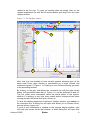
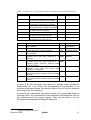
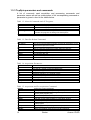
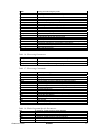
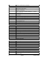

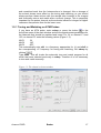
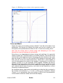
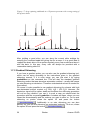
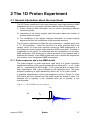
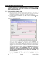
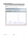
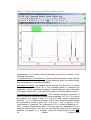

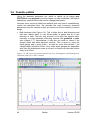
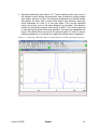
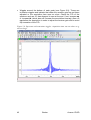
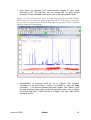
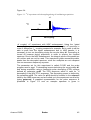
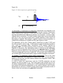
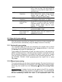
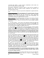

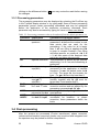
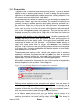


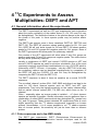
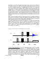
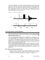
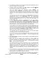


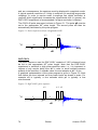
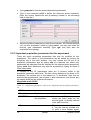

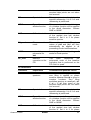
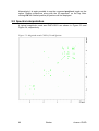
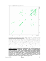
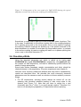
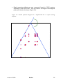
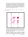

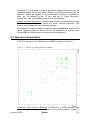
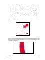
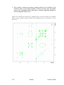
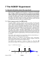
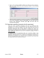

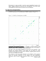
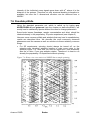

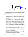
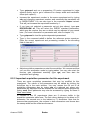

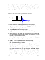

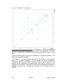

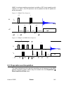
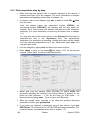
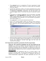

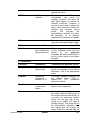
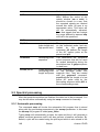
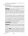

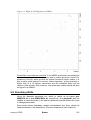
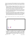
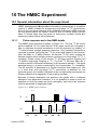
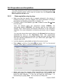

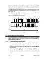
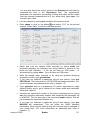


![e-track User`s Manual [FW1.00]](http://vs1.manualzilla.com/store/data/005696177_1-79f2a7130a6208690505d356432cfe5f-150x150.png)