1
Webots User Guide
release 8.3.2
c 2015 Cyberbotics Ltd.
Copyright All Rights Reserved
www.cyberbotics.com
December 16, 2015
2
Permission to use, copy and distribute this documentation for any purpose and without fee is
hereby granted in perpetuity, provided that no modifications are performed on this documentation.
The copyright holder makes no warranty or condition, either expressed or implied, including
but not limited to any implied warranties of merchantability and fitness for a particular purpose,
regarding this manual and the associated software. This manual is provided on an as-is basis.
Neither the copyright holder nor any applicable licensor will be liable for any incidental or consequential damages.
The Webots software was initially developed at the Laboratoire de Micro-Informatique (LAMI)
of the Swiss Federal Institute of Technology, Lausanne, Switzerland (EPFL). The EPFL makes
no warranties of any kind on this software. In no event shall the EPFL be liable for incidental or
consequential damages of any kind in connection with the use and exploitation of this software.
Trademark information
AiboTM is a registered trademark of SONY Corp.
RadeonTM is a registered trademark of ATI Technologies Inc.
GeForceTM is a registered trademark of nVidia, Corp.
JavaTM is a registered trademark of Sun MicroSystems, Inc.
KheperaTM and KoalaTM are registered trademarks of K-Team S.A.
LinuxTM is a registered trademark of Linus Torvalds.
Mac OS XTM is a registered trademark of Apple Inc.
MindstormsTM and LEGOTM are registered trademarks of the LEGO group.
IPRTM is a registered trademark of Neuronics AG.
UbuntuTM is a registered trademark of Canonical Ltd.
Visual C++TM , WindowsTM , Windows NTTM , Windows 2000TM , Windows XPTM , Windows
VistaTM , Windows 7TM and Windows 8TM are registered trademarks of Microsoft Corp.
UNIXTM is a registered trademark licensed exclusively by X/Open Company, Ltd.
Foreword
Webots is a three-dimensional mobile robot simulator. It was originally developed as a research
tool for investigating various control algorithms in mobile robotics.
This user guide will get you started using Webots. However, the reader is expected to have a
minimal knowledge in mobile robotics, in C, C++, Java, Python or MATLAB programming, and
in VRML97 (Virtual Reality Modeling Language).
Webots 8 features a new layout of the user interface with many facilities integrated, such as a
source code editor, motion editor, etc.
We hope that you will enjoy working with Webots 8.
3
4
Thanks
Cyberbotics is grateful to all the people who contributed to the development of Webots, Webots
sample applications, the Webots User Guide, the Webots Reference Manual, and the Webots
web site, including Stefania Pedrazzi, David Mansolino, Yvan Bourquin, Fabien Rohrer, JeanChristophe Fillion-Robin, Jordi Porta, Emanuele Ornella, Yuri Lopez de Meneses, Sébastien
Hugues, Auke-Jan Ispeert, Jonas Buchli, Alessandro Crespi, Ludovic Righetti, Julien Gagnet, Lukas Hohl, Pascal Cominoli, Stéphane Mojon, Jérôme Braure, Sergei Poskriakov, Anthony Truchet, Alcherio Martinoli, Chris Cianci, Nikolaus Correll, Jim Pugh, Yizhen Zhang,
Anne-Elisabeth Tran Qui, Grégory Mermoud, Lucien Epinet, Jean-Christophe Zufferey, Laurent
Lessieux, Aude Billiard, Ricardo Tellez, Gerald Foliot, Allen Johnson, Michael Kertesz, Simon
Garnieri, Simon Blanchoud, Manuel João Ferreira, Rui Picas, José Afonso Pires, Cristina Santos,
Michal Pytasz and many others.
Moreover, many thanks are due to Cyberbotics’s Mentors: Prof. Jean-Daniel Nicoud (LAMIEPFL), Dr. Francesco Mondada (EPFL), Dr. Takashi Gomi (Applied AI, Inc.).
Finally, thanks to Skye Legon and Nathan Yawn, who proofread this guide.
5
6
Contents
1
Installing Webots
1.1
19
Webots licenses . . . . . . . . . . . . . . . . . . . . . . . . . . . . . . . . . . . 19
1.1.1
Webots PRO . . . . . . . . . . . . . . . . . . . . . . . . . . . . . . . . 19
1.1.2
Webots EDU . . . . . . . . . . . . . . . . . . . . . . . . . . . . . . . . 19
1.1.3
Webots MOD . . . . . . . . . . . . . . . . . . . . . . . . . . . . . . . . 20
1.1.4
Webots licences overview . . . . . . . . . . . . . . . . . . . . . . . . . 20
1.2
System requirements . . . . . . . . . . . . . . . . . . . . . . . . . . . . . . . . 20
1.3
Verifying your graphics driver installation . . . . . . . . . . . . . . . . . . . . . 21
1.4
1.5
1.6
1.3.1
Supported graphics cards . . . . . . . . . . . . . . . . . . . . . . . . . . 21
1.3.2
Unsupported graphics cards . . . . . . . . . . . . . . . . . . . . . . . . 21
1.3.3
Upgrading your graphics driver . . . . . . . . . . . . . . . . . . . . . . 22
1.3.4
Hardware acceleration tips . . . . . . . . . . . . . . . . . . . . . . . . . 23
Installation procedure . . . . . . . . . . . . . . . . . . . . . . . . . . . . . . . . 24
1.4.1
Linux . . . . . . . . . . . . . . . . . . . . . . . . . . . . . . . . . . . . 24
1.4.2
Windows . . . . . . . . . . . . . . . . . . . . . . . . . . . . . . . . . . 26
1.4.3
Mac OS X . . . . . . . . . . . . . . . . . . . . . . . . . . . . . . . . . 27
Webots license system . . . . . . . . . . . . . . . . . . . . . . . . . . . . . . . 27
1.5.1
Firewall configuration (optional) . . . . . . . . . . . . . . . . . . . . . . 27
1.5.2
License agreement . . . . . . . . . . . . . . . . . . . . . . . . . . . . . 28
1.5.3
License setup . . . . . . . . . . . . . . . . . . . . . . . . . . . . . . . . 28
1.5.4
License administration . . . . . . . . . . . . . . . . . . . . . . . . . . . 28
1.5.5
Module download folder . . . . . . . . . . . . . . . . . . . . . . . . . . 28
Classroom license setup . . . . . . . . . . . . . . . . . . . . . . . . . . . . . . . 29
7
8
CONTENTS
1.7
2
1.6.1
User account . . . . . . . . . . . . . . . . . . . . . . . . . . . . . . . . 29
1.6.2
Classrom . . . . . . . . . . . . . . . . . . . . . . . . . . . . . . . . . . 31
1.6.3
Homework . . . . . . . . . . . . . . . . . . . . . . . . . . . . . . . . . 31
1.6.4
Using Webots without Internet connection . . . . . . . . . . . . . . . . . 32
Translating Webots to your own language . . . . . . . . . . . . . . . . . . . . . 32
Getting Started with Webots
2.1
2.2
2.3
33
Introduction to Webots . . . . . . . . . . . . . . . . . . . . . . . . . . . . . . . 33
2.1.1
What is Webots? . . . . . . . . . . . . . . . . . . . . . . . . . . . . . . 33
2.1.2
What can I do with Webots? . . . . . . . . . . . . . . . . . . . . . . . . 33
2.1.3
What do I need to know to use Webots? . . . . . . . . . . . . . . . . . . 34
2.1.4
Webots simulation . . . . . . . . . . . . . . . . . . . . . . . . . . . . . 34
2.1.5
What is a world? . . . . . . . . . . . . . . . . . . . . . . . . . . . . . . 35
2.1.6
What is a controller? . . . . . . . . . . . . . . . . . . . . . . . . . . . . 35
2.1.7
What is a Supervisor? . . . . . . . . . . . . . . . . . . . . . . . . . . . 35
Starting Webots . . . . . . . . . . . . . . . . . . . . . . . . . . . . . . . . . . . 36
2.2.1
Linux . . . . . . . . . . . . . . . . . . . . . . . . . . . . . . . . . . . . 36
2.2.2
Mac OS X . . . . . . . . . . . . . . . . . . . . . . . . . . . . . . . . . 36
2.2.3
Windows . . . . . . . . . . . . . . . . . . . . . . . . . . . . . . . . . . 36
2.2.4
Command Line Arguments . . . . . . . . . . . . . . . . . . . . . . . . . 36
The User Interface . . . . . . . . . . . . . . . . . . . . . . . . . . . . . . . . . 38
2.3.1
File Menu . . . . . . . . . . . . . . . . . . . . . . . . . . . . . . . . . . 38
2.3.2
Edit Menu
2.3.3
View Menu . . . . . . . . . . . . . . . . . . . . . . . . . . . . . . . . . 41
2.3.4
Simulation Menu . . . . . . . . . . . . . . . . . . . . . . . . . . . . . . 43
2.3.5
Build Menu . . . . . . . . . . . . . . . . . . . . . . . . . . . . . . . . . 44
2.3.6
Robot Menu . . . . . . . . . . . . . . . . . . . . . . . . . . . . . . . . 44
2.3.7
Tools Menu . . . . . . . . . . . . . . . . . . . . . . . . . . . . . . . . . 45
2.3.8
Wizards Menu . . . . . . . . . . . . . . . . . . . . . . . . . . . . . . . 45
2.3.9
Help menu . . . . . . . . . . . . . . . . . . . . . . . . . . . . . . . . . 46
. . . . . . . . . . . . . . . . . . . . . . . . . . . . . . . . . 41
2.3.10 Main toolbar . . . . . . . . . . . . . . . . . . . . . . . . . . . . . . . . 46
CONTENTS
9
2.3.11 Speedometer and Virtual Time . . . . . . . . . . . . . . . . . . . . . . . 47
2.4
2.5
The 3D Window . . . . . . . . . . . . . . . . . . . . . . . . . . . . . . . . . . . 47
2.4.1
Selecting an object . . . . . . . . . . . . . . . . . . . . . . . . . . . . . 47
2.4.2
Navigation in the scene . . . . . . . . . . . . . . . . . . . . . . . . . . . 48
2.4.3
Moving a solid object . . . . . . . . . . . . . . . . . . . . . . . . . . . . 48
2.4.4
Applying a force to a solid object with physics . . . . . . . . . . . . . . 49
2.4.5
Applying a torque to a solid object with physics . . . . . . . . . . . . . . 50
2.4.6
Moving and resizing Overlays . . . . . . . . . . . . . . . . . . . . . . . 50
2.4.7
Show Camera and Display images in separate window . . . . . . . . . . 50
The Scene Tree . . . . . . . . . . . . . . . . . . . . . . . . . . . . . . . . . . . 52
2.5.1
2.6
2.7
3
Field Editor . . . . . . . . . . . . . . . . . . . . . . . . . . . . . . . . . 52
Preferences . . . . . . . . . . . . . . . . . . . . . . . . . . . . . . . . . . . . . 54
2.6.1
General . . . . . . . . . . . . . . . . . . . . . . . . . . . . . . . . . . . 55
2.6.2
OpenGL . . . . . . . . . . . . . . . . . . . . . . . . . . . . . . . . . . . 55
Citing Webots . . . . . . . . . . . . . . . . . . . . . . . . . . . . . . . . . . . . 56
2.7.1
Citing Cyberbotics’ web site . . . . . . . . . . . . . . . . . . . . . . . . 56
2.7.2
Citing a reference journal paper about Webots . . . . . . . . . . . . . . . 56
Sample Webots Applications
3.1
59
Samples . . . . . . . . . . . . . . . . . . . . . . . . . . . . . . . . . . . . . . . 59
3.1.1
blimp lis.wbt . . . . . . . . . . . . . . . . . . . . . . . . . . . . . . . . 60
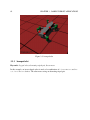
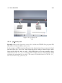
3.1.2
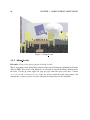
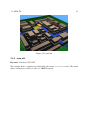
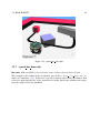
gantry.wbt . . . . . . . . . . . . . . . . . . . . . . . . . . . . . . . . . . 61
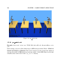
3.1.3
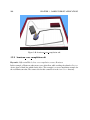
hexapod.wbt . . . . . . . . . . . . . . . . . . . . . . . . . . . . . . . . 62
3.1.4
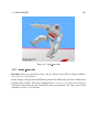
humanoid.wbt
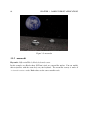
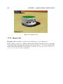
3.1.5
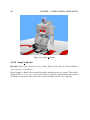
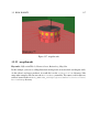
moon.wbt . . . . . . . . . . . . . . . . . . . . . . . . . . . . . . . . . . 64
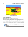
3.1.6
ghostdog.wbt . . . . . . . . . . . . . . . . . . . . . . . . . . . . . . . . 65
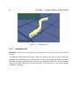
3.1.7
salamander.wbt . . . . . . . . . . . . . . . . . . . . . . . . . . . . . . . 66
3.1.8
soccer.wbt . . . . . . . . . . . . . . . . . . . . . . . . . . . . . . . . . . 67
3.1.9
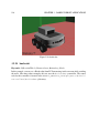
sojourner.wbt . . . . . . . . . . . . . . . . . . . . . . . . . . . . . . . . 68
3.1.10 yamor.wbt
. . . . . . . . . . . . . . . . . . . . . . . . . . . . . . . 63
. . . . . . . . . . . . . . . . . . . . . . . . . . . . . . . . . 69
3.1.11 stewart platform.wbt . . . . . . . . . . . . . . . . . . . . . . . . . . . . 70
10
CONTENTS
3.2
Webots Devices . . . . . . . . . . . . . . . . . . . . . . . . . . . . . . . . . . . 71
3.2.1
battery.wbt . . . . . . . . . . . . . . . . . . . . . . . . . . . . . . . . . 71
3.2.2
bumper.wbt . . . . . . . . . . . . . . . . . . . . . . . . . . . . . . . . . 72
3.2.3
camera.wbt . . . . . . . . . . . . . . . . . . . . . . . . . . . . . . . . . 73
3.2.4
connector.wbt . . . . . . . . . . . . . . . . . . . . . . . . . . . . . . . . 74
3.2.5
distance sensor.wbt . . . . . . . . . . . . . . . . . . . . . . . . . . . . . 75
3.2.6
emitter receiver.wbt . . . . . . . . . . . . . . . . . . . . . . . . . . . . 76
3.2.7
encoders.wbt . . . . . . . . . . . . . . . . . . . . . . . . . . . . . . . . 77
3.2.8
force sensor.wbt . . . . . . . . . . . . . . . . . . . . . . . . . . . . . . 78
3.2.9
gps.wbt . . . . . . . . . . . . . . . . . . . . . . . . . . . . . . . . . . . 79
3.2.10 led.wbt . . . . . . . . . . . . . . . . . . . . . . . . . . . . . . . . . . . 80
3.2.11 light sensor.wbt . . . . . . . . . . . . . . . . . . . . . . . . . . . . . . . 81
3.2.12 pen.wbt . . . . . . . . . . . . . . . . . . . . . . . . . . . . . . . . . . . 82
3.2.13 range finder.wbt . . . . . . . . . . . . . . . . . . . . . . . . . . . . . . 83
3.3
How To . . . . . . . . . . . . . . . . . . . . . . . . . . . . . . . . . . . . . . . 84
3.3.1
binocular.wbt . . . . . . . . . . . . . . . . . . . . . . . . . . . . . . . . 84
3.3.2
biped.wbt . . . . . . . . . . . . . . . . . . . . . . . . . . . . . . . . . . 85
3.3.3
force control.wbt . . . . . . . . . . . . . . . . . . . . . . . . . . . . . . 86
3.3.4
inverted pendulum.wbt . . . . . . . . . . . . . . . . . . . . . . . . . . . 87
3.3.5
physics.wbt . . . . . . . . . . . . . . . . . . . . . . . . . . . . . . . . . 88
3.3.6
supervisor.wbt . . . . . . . . . . . . . . . . . . . . . . . . . . . . . . . 89
3.3.7
texture change.wbt . . . . . . . . . . . . . . . . . . . . . . . . . . . . . 90
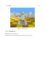
3.3.8
town.wbt . . . . . . . . . . . . . . . . . . . . . . . . . . . . . . . . . . 91
3.4
Geometries . . . . . . . . . . . . . . . . . . . . . . . . . . . . . . . . . . . . . 92
3.5
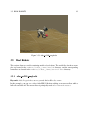
Real Robots . . . . . . . . . . . . . . . . . . . . . . . . . . . . . . . . . . . . . 93
3.5.1
aibo ers210 rough.wbt . . . . . . . . . . . . . . . . . . . . . . . . . . . 93
3.5.2
aibo ers7.wbt . . . . . . . . . . . . . . . . . . . . . . . . . . . . . . . . 94
3.5.3
alice.wbt . . . . . . . . . . . . . . . . . . . . . . . . . . . . . . . . . . 95
3.5.4
boebot.wbt . . . . . . . . . . . . . . . . . . . . . . . . . . . . . . . . . 96
3.5.5
e-puck.wbt . . . . . . . . . . . . . . . . . . . . . . . . . . . . . . . . . 97
3.5.6
e-puck line.wbt . . . . . . . . . . . . . . . . . . . . . . . . . . . . . . . 98
CONTENTS
11
3.5.7
e-puck line demo.wbt . . . . . . . . . . . . . . . . . . . . . . . . . . . 99
3.5.8
hemisson cross compilation.wbt . . . . . . . . . . . . . . . . . . . . . . 100
3.5.9
hoap2 sumo.wbt . . . . . . . . . . . . . . . . . . . . . . . . . . . . . . 101
3.5.10 hoap2 walk.wbt . . . . . . . . . . . . . . . . . . . . . . . . . . . . . . . 102
3.5.11 ipr collaboration.wbt . . . . . . . . . . . . . . . . . . . . . . . . . . . . 103
3.5.12 ipr cube.wbt . . . . . . . . . . . . . . . . . . . . . . . . . . . . . . . . 104
3.5.13 ipr factory.wbt . . . . . . . . . . . . . . . . . . . . . . . . . . . . . . . 105
3.5.14 ipr models.wbt . . . . . . . . . . . . . . . . . . . . . . . . . . . . . . . 106
3.5.15 khepera.wbt . . . . . . . . . . . . . . . . . . . . . . . . . . . . . . . . . 107
3.5.16 khepera2.wbt . . . . . . . . . . . . . . . . . . . . . . . . . . . . . . . . 108
3.5.17 khepera3.wbt . . . . . . . . . . . . . . . . . . . . . . . . . . . . . . . . 109
3.5.18 khepera kinematic.wbt . . . . . . . . . . . . . . . . . . . . . . . . . . . 110
3.5.19 khepera gripper.wbt . . . . . . . . . . . . . . . . . . . . . . . . . . . . 111
3.5.20 khepera gripper camera.wbt . . . . . . . . . . . . . . . . . . . . . . . . 112
3.5.21 khepera k213.wbt . . . . . . . . . . . . . . . . . . . . . . . . . . . . . 113
3.5.22 khepera pipe.wbt . . . . . . . . . . . . . . . . . . . . . . . . . . . . . . 114
3.5.23 khepera tcpip.wbt . . . . . . . . . . . . . . . . . . . . . . . . . . . . . 115
3.5.24 koala.wbt . . . . . . . . . . . . . . . . . . . . . . . . . . . . . . . . . . 116
3.5.25 magellan.wbt . . . . . . . . . . . . . . . . . . . . . . . . . . . . . . . . 117
3.5.26 pioneer2.wbt . . . . . . . . . . . . . . . . . . . . . . . . . . . . . . . . 118
3.5.27 rover.wbt . . . . . . . . . . . . . . . . . . . . . . . . . . . . . . . . . . 119
3.5.28 scout2.wbt . . . . . . . . . . . . . . . . . . . . . . . . . . . . . . . . . 120
3.5.29 shrimp.wbt . . . . . . . . . . . . . . . . . . . . . . . . . . . . . . . . . 121
3.5.30 bioloid.wbt . . . . . . . . . . . . . . . . . . . . . . . . . . . . . . . . . 122
4
Language Setup
125
4.1
Introduction . . . . . . . . . . . . . . . . . . . . . . . . . . . . . . . . . . . . . 125
4.2
Controller Start-up . . . . . . . . . . . . . . . . . . . . . . . . . . . . . . . . . 125
4.3
Using C . . . . . . . . . . . . . . . . . . . . . . . . . . . . . . . . . . . . . . . 126
4.3.1
Introduction . . . . . . . . . . . . . . . . . . . . . . . . . . . . . . . . . 126
4.3.2
C/C++ Compiler Installation . . . . . . . . . . . . . . . . . . . . . . . . 127
12
CONTENTS
4.4
4.5
4.6
4.7
4.8
4.9
5
Using C++ . . . . . . . . . . . . . . . . . . . . . . . . . . . . . . . . . . . . . . 127
4.4.1
Introduction . . . . . . . . . . . . . . . . . . . . . . . . . . . . . . . . . 127
4.4.2
C++ Compiler Installation . . . . . . . . . . . . . . . . . . . . . . . . . 128
4.4.3
Source Code of the C++ API . . . . . . . . . . . . . . . . . . . . . . . . 128
Using Java . . . . . . . . . . . . . . . . . . . . . . . . . . . . . . . . . . . . . . 128
4.5.1
Introduction . . . . . . . . . . . . . . . . . . . . . . . . . . . . . . . . . 128
4.5.2
Java and Java Compiler Installation . . . . . . . . . . . . . . . . . . . . 128
4.5.3
Link with external jar files . . . . . . . . . . . . . . . . . . . . . . . . . 130
4.5.4
Source Code of the Java API . . . . . . . . . . . . . . . . . . . . . . . . 130
Using Python . . . . . . . . . . . . . . . . . . . . . . . . . . . . . . . . . . . . 131
4.6.1
Introduction . . . . . . . . . . . . . . . . . . . . . . . . . . . . . . . . . 131
4.6.2
Python Installation . . . . . . . . . . . . . . . . . . . . . . . . . . . . . 131
4.6.3
Source Code of the Python API . . . . . . . . . . . . . . . . . . . . . . 132
Using MATLAB . . . . . . . . . . . . . . . . . . . . . . . . . . . . . . . . . . 132
4.7.1
Introduction to MATLABTM . . . . . . . . . . . . . . . . . . . . . . . . 132
4.7.2
How to run the Examples? . . . . . . . . . . . . . . . . . . . . . . . . . 132
4.7.3
MATLABTM Installation . . . . . . . . . . . . . . . . . . . . . . . . . . 133
4.7.4
Display information to Webots console . . . . . . . . . . . . . . . . . . 133
4.7.5
Compatibility Issues . . . . . . . . . . . . . . . . . . . . . . . . . . . . 134
Using ROS . . . . . . . . . . . . . . . . . . . . . . . . . . . . . . . . . . . . . 134
4.8.1
What is ROS? . . . . . . . . . . . . . . . . . . . . . . . . . . . . . . . . 134
4.8.2
ROS for Webots . . . . . . . . . . . . . . . . . . . . . . . . . . . . . . 135
Interfacing Webots to third party software with TCP/IP . . . . . . . . . . . . . . 137
4.9.1
Overview . . . . . . . . . . . . . . . . . . . . . . . . . . . . . . . . . . 137
4.9.2
Main advantages . . . . . . . . . . . . . . . . . . . . . . . . . . . . . . 137
4.9.3
Limitations . . . . . . . . . . . . . . . . . . . . . . . . . . . . . . . . . 138
Development Environments
5.1
Webots Built-in Editor . . . . . . . . . . . . . . . . . . . . . . . . . . . . . . . 139
5.1.1
5.2
139
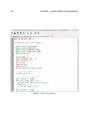
Compiling with the Source Code Editor . . . . . . . . . . . . . . . . . . 139
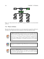
The standard File Hierarchy of a Project . . . . . . . . . . . . . . . . . . . . . . 141
CONTENTS
5.3
5.4
5.5
5.6
5.7
5.8
6
13
5.2.1
The Root Directory of a Project . . . . . . . . . . . . . . . . . . . . . . 141
5.2.2
The Project Files . . . . . . . . . . . . . . . . . . . . . . . . . . . . . . 142
5.2.3
The ”controllers” Directory . . . . . . . . . . . . . . . . . . . . . . . . 142
Compiling Controllers in a Terminal . . . . . . . . . . . . . . . . . . . . . . . . 142
5.3.1
Mac OS X and Linux . . . . . . . . . . . . . . . . . . . . . . . . . . . . 142
5.3.2
Windows . . . . . . . . . . . . . . . . . . . . . . . . . . . . . . . . . . 143
Using Webots Makefiles . . . . . . . . . . . . . . . . . . . . . . . . . . . . . . 143
5.4.1
What are Makefiles . . . . . . . . . . . . . . . . . . . . . . . . . . . . . 143
5.4.2
Controller with Several Source Files (C/C++) . . . . . . . . . . . . . . . 144
5.4.3
Using the Compiler and Linker Flags (C/C++) . . . . . . . . . . . . . . 144
Debugging C/C++ Controllers . . . . . . . . . . . . . . . . . . . . . . . . . . . 146
5.5.1
Controller processes . . . . . . . . . . . . . . . . . . . . . . . . . . . . 146
5.5.2
Using the GNU debugger with a controller . . . . . . . . . . . . . . . . 147
Using Visual C++ with Webots . . . . . . . . . . . . . . . . . . . . . . . . . . . 148
5.6.1
Introduction . . . . . . . . . . . . . . . . . . . . . . . . . . . . . . . . . 148
5.6.2
Configuration . . . . . . . . . . . . . . . . . . . . . . . . . . . . . . . . 149
Starting Webots Remotely (ssh) . . . . . . . . . . . . . . . . . . . . . . . . . . 151
5.7.1
Using the ssh command . . . . . . . . . . . . . . . . . . . . . . . . . . 151
5.7.2
Terminating the ssh session . . . . . . . . . . . . . . . . . . . . . . . . 152
Transfer to your own robot . . . . . . . . . . . . . . . . . . . . . . . . . . . . . 152
5.8.1
Remote control . . . . . . . . . . . . . . . . . . . . . . . . . . . . . . . 153
5.8.2
Cross-compilation . . . . . . . . . . . . . . . . . . . . . . . . . . . . . 154
5.8.3
Interpreted language . . . . . . . . . . . . . . . . . . . . . . . . . . . . 154
Programming Fundamentals
6.1
155
Controller Programming . . . . . . . . . . . . . . . . . . . . . . . . . . . . . . 155
6.1.1
Hello World Example . . . . . . . . . . . . . . . . . . . . . . . . . . . 155
6.1.2
Reading Sensors . . . . . . . . . . . . . . . . . . . . . . . . . . . . . . 156
6.1.3
Using Actuators . . . . . . . . . . . . . . . . . . . . . . . . . . . . . . 158
6.1.4
How to use wb robot step() . . . . . . . . . . . . . . . . . . . . . . . . 160
6.1.5
Using Sensors and Actuators Together . . . . . . . . . . . . . . . . . . . 160
14
CONTENTS
6.1.6
Using Controller Arguments . . . . . . . . . . . . . . . . . . . . . . . . 162
6.1.7
Controller Termination . . . . . . . . . . . . . . . . . . . . . . . . . . . 163
6.1.8
Shared libraries . . . . . . . . . . . . . . . . . . . . . . . . . . . . . . . 165
6.1.9
Environment variables . . . . . . . . . . . . . . . . . . . . . . . . . . . 165
6.1.10 Languages settings . . . . . . . . . . . . . . . . . . . . . . . . . . . . . 167
6.2
6.3
6.4
6.5
Supervisor Programming . . . . . . . . . . . . . . . . . . . . . . . . . . . . . . 167
6.2.1
Introduction . . . . . . . . . . . . . . . . . . . . . . . . . . . . . . . . . 168
6.2.2
Tracking the Position of Robots . . . . . . . . . . . . . . . . . . . . . . 168
6.2.3
Setting the Position of Robots . . . . . . . . . . . . . . . . . . . . . . . 169
Using Numerical Optimization Methods . . . . . . . . . . . . . . . . . . . . . . 171
6.3.1
Choosing the correct Supervisor approach . . . . . . . . . . . . . . . . . 171
6.3.2
Resetting the robot . . . . . . . . . . . . . . . . . . . . . . . . . . . . . 173
C++/Java/Python . . . . . . . . . . . . . . . . . . . . . . . . . . . . . . . . . . 176
6.4.1
Classes and Methods . . . . . . . . . . . . . . . . . . . . . . . . . . . . 177
6.4.2
Controller Class . . . . . . . . . . . . . . . . . . . . . . . . . . . . . . 177
6.4.3
C++ Example . . . . . . . . . . . . . . . . . . . . . . . . . . . . . . . . 179
6.4.4
Java Example . . . . . . . . . . . . . . . . . . . . . . . . . . . . . . . . 180
6.4.5
Python Example . . . . . . . . . . . . . . . . . . . . . . . . . . . . . . 181
Matlab . . . . . . . . . . . . . . . . . . . . . . . . . . . . . . . . . . . . . . . . 181
6.5.1
6.6
6.7
Using the MATLABTM desktop . . . . . . . . . . . . . . . . . . . . . . . 182
Controller Plugin . . . . . . . . . . . . . . . . . . . . . . . . . . . . . . . . . . 183
6.6.1
Fundamentals . . . . . . . . . . . . . . . . . . . . . . . . . . . . . . . . 183
6.6.2
Robot Window Plugin . . . . . . . . . . . . . . . . . . . . . . . . . . . 184
6.6.3
Qt utility library . . . . . . . . . . . . . . . . . . . . . . . . . . . . . . 186
6.6.4
Motion editor . . . . . . . . . . . . . . . . . . . . . . . . . . . . . . . . 187
6.6.5
Remote-control Plugin . . . . . . . . . . . . . . . . . . . . . . . . . . . 188
Webots Plugin . . . . . . . . . . . . . . . . . . . . . . . . . . . . . . . . . . . . 189
6.7.1
Physics Plugin . . . . . . . . . . . . . . . . . . . . . . . . . . . . . . . 190
CONTENTS
7
Tutorials
7.1
7.2
7.3
7.4
7.5
15
191
Prerequisites . . . . . . . . . . . . . . . . . . . . . . . . . . . . . . . . . . . . . 192
7.1.1
Install Webots . . . . . . . . . . . . . . . . . . . . . . . . . . . . . . . . 192
7.1.2
Create a directory for all your Webots files . . . . . . . . . . . . . . . . 192
7.1.3
Start Webots . . . . . . . . . . . . . . . . . . . . . . . . . . . . . . . . 192
7.1.4
Create a new Project . . . . . . . . . . . . . . . . . . . . . . . . . . . . 193
7.1.5
The Webots Graphical User Interface (GUI) . . . . . . . . . . . . . . . . 193
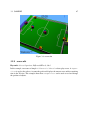
Tutorial 1: Your first Simulation in Webots (20 minutes) . . . . . . . . . . . . . 193
7.2.1
Create a new World . . . . . . . . . . . . . . . . . . . . . . . . . . . . . 195
7.2.2
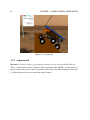
Add an e-puck Robot . . . . . . . . . . . . . . . . . . . . . . . . . . . . 197
7.2.3
Create a new Controller . . . . . . . . . . . . . . . . . . . . . . . . . . 199
7.2.4
Conclusion . . . . . . . . . . . . . . . . . . . . . . . . . . . . . . . . . 201
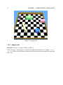
Tutorial 2: Modification of the Environment (20 minutes) . . . . . . . . . . . . . 201
7.3.1
A new Simulation . . . . . . . . . . . . . . . . . . . . . . . . . . . . . 201
7.3.2
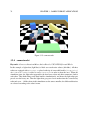
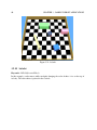
Modification of the Floor . . . . . . . . . . . . . . . . . . . . . . . . . . 201
7.3.3
The Solid Node . . . . . . . . . . . . . . . . . . . . . . . . . . . . . . . 202
7.3.4
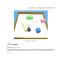
Create a Ball . . . . . . . . . . . . . . . . . . . . . . . . . . . . . . . . 203
7.3.5
Geometries . . . . . . . . . . . . . . . . . . . . . . . . . . . . . . . . . 204
7.3.6
DEF-USE mechanism . . . . . . . . . . . . . . . . . . . . . . . . . . . 204
7.3.7
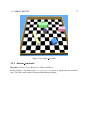
Add Walls . . . . . . . . . . . . . . . . . . . . . . . . . . . . . . . . . . 205
7.3.8
Efficiency . . . . . . . . . . . . . . . . . . . . . . . . . . . . . . . . . . 207
7.3.9
Conclusion . . . . . . . . . . . . . . . . . . . . . . . . . . . . . . . . . 207
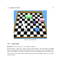
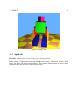
Tutorial 3: Appearance (15 minutes) . . . . . . . . . . . . . . . . . . . . . . . . 208
7.4.1
New simulation . . . . . . . . . . . . . . . . . . . . . . . . . . . . . . . 208
7.4.2
Lights . . . . . . . . . . . . . . . . . . . . . . . . . . . . . . . . . . . . 208
7.4.3
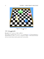
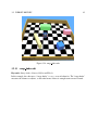
Modify the Appearance of the Walls . . . . . . . . . . . . . . . . . . . . 209
7.4.4
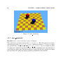
Add a Texture to the Ball . . . . . . . . . . . . . . . . . . . . . . . . . . 209
7.4.5
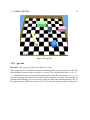
Rendering Options . . . . . . . . . . . . . . . . . . . . . . . . . . . . . 210
7.4.6
Conclusion . . . . . . . . . . . . . . . . . . . . . . . . . . . . . . . . . 210
Tutorial 4: More about Controllers (20 minutes) . . . . . . . . . . . . . . . . . . 210
7.5.1
New World and new Controller . . . . . . . . . . . . . . . . . . . . . . 211
16
CONTENTS
7.6
7.7
7.8
7.9
8
7.5.2
Understand the e-puck Model . . . . . . . . . . . . . . . . . . . . . . . 211
7.5.3
Program a Controller . . . . . . . . . . . . . . . . . . . . . . . . . . . . 212
7.5.4
The Controller Code . . . . . . . . . . . . . . . . . . . . . . . . . . . . 216
7.5.5
Conclusion . . . . . . . . . . . . . . . . . . . . . . . . . . . . . . . . . 218
Tutorial 5: Compound Solid and Physics Attributes (15 minutes) . . . . . . . . . 218
7.6.1
New simulation . . . . . . . . . . . . . . . . . . . . . . . . . . . . . . . 219
7.6.2
Compound Solid . . . . . . . . . . . . . . . . . . . . . . . . . . . . . . 219
7.6.3
Physics Attributes . . . . . . . . . . . . . . . . . . . . . . . . . . . . . 220
7.6.4
The Rotation Field . . . . . . . . . . . . . . . . . . . . . . . . . . . . . 221
7.6.5
How to choose bounding Objects? . . . . . . . . . . . . . . . . . . . . . 221
7.6.6
Contacts
7.6.7
basicTimeStep, ERP and CFM . . . . . . . . . . . . . . . . . . . . . . . 222
7.6.8
Minor physics Parameters . . . . . . . . . . . . . . . . . . . . . . . . . 222
7.6.9
Conclusion . . . . . . . . . . . . . . . . . . . . . . . . . . . . . . . . . 223
Tutorial 6: 4-Wheels Robot . . . . . . . . . . . . . . . . . . . . . . . . . . . . . 223
7.7.1
New simulation . . . . . . . . . . . . . . . . . . . . . . . . . . . . . . . 223
7.7.2
Separating the Robot in Solid Nodes . . . . . . . . . . . . . . . . . . . . 223
7.7.3
HingeJoints . . . . . . . . . . . . . . . . . . . . . . . . . . . . . . . . . 226
7.7.4
Sensors . . . . . . . . . . . . . . . . . . . . . . . . . . . . . . . . . . . 227
7.7.5
Controller . . . . . . . . . . . . . . . . . . . . . . . . . . . . . . . . . . 227
7.7.6
Conclusion . . . . . . . . . . . . . . . . . . . . . . . . . . . . . . . . . 228
Tutorial 7: Using ROS . . . . . . . . . . . . . . . . . . . . . . . . . . . . . . . 229
7.8.1
Creating a Webots project that contains a ROS package . . . . . . . . . . 229
7.8.2
Conclusion . . . . . . . . . . . . . . . . . . . . . . . . . . . . . . . . . 233
Going Further . . . . . . . . . . . . . . . . . . . . . . . . . . . . . . . . . . . . 233
Robots
8.1
. . . . . . . . . . . . . . . . . . . . . . . . . . . . . . . . . . 222
235
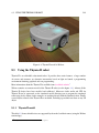
Using the e-puck robot . . . . . . . . . . . . . . . . . . . . . . . . . . . . . . . 235
8.1.1
Overview of the robot . . . . . . . . . . . . . . . . . . . . . . . . . . . 235
8.1.2
Simulation model . . . . . . . . . . . . . . . . . . . . . . . . . . . . . . 236
8.1.3
Control interface . . . . . . . . . . . . . . . . . . . . . . . . . . . . . . 240
CONTENTS
8.2
8.3
8.4
9
Using the Nao robot . . . . . . . . . . . . . . . . . . . . . . . . . . . . . . . . . 245
8.2.1
Introduction . . . . . . . . . . . . . . . . . . . . . . . . . . . . . . . . . 245
8.2.2
Using Webots with Choregraphe . . . . . . . . . . . . . . . . . . . . . . 245
8.2.3
Nao models . . . . . . . . . . . . . . . . . . . . . . . . . . . . . . . . . 246
8.2.4
Using motion boxes . . . . . . . . . . . . . . . . . . . . . . . . . . . . 246
8.2.5
Using the cameras . . . . . . . . . . . . . . . . . . . . . . . . . . . . . 247
8.2.6
Using Several Nao robots . . . . . . . . . . . . . . . . . . . . . . . . . 247
8.2.7
Getting the right speed for realistic simulation . . . . . . . . . . . . . . . 248
8.2.8
Known Problems . . . . . . . . . . . . . . . . . . . . . . . . . . . . . . 248
Using the Thymio II robot . . . . . . . . . . . . . . . . . . . . . . . . . . . . . 249
8.3.1
Thymio II model . . . . . . . . . . . . . . . . . . . . . . . . . . . . . . 249
8.3.2
Connect Aseba to the Thymio II model . . . . . . . . . . . . . . . . . . 250
8.3.3
Thymio II Pen . . . . . . . . . . . . . . . . . . . . . . . . . . . . . . . 251
8.3.4
Thymio II Ball . . . . . . . . . . . . . . . . . . . . . . . . . . . . . . . 253
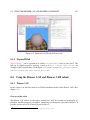
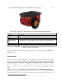
Using the Pioneer 3-AT and Pioneer 3-DX robots . . . . . . . . . . . . . . . . . 253
8.4.1
Pioneer 3-AT . . . . . . . . . . . . . . . . . . . . . . . . . . . . . . . . 253
8.4.2
Pioneer 3-DX . . . . . . . . . . . . . . . . . . . . . . . . . . . . . . . . 256
Webots FAQ
9.1
9.2
17
261
General FAQ . . . . . . . . . . . . . . . . . . . . . . . . . . . . . . . . . . . . 261
9.1.1
What are the differences between Webots PRO, Webots EDU and other
Webots modules? . . . . . . . . . . . . . . . . . . . . . . . . . . . . . . 261
9.1.2
How can I report a bug in Webots? . . . . . . . . . . . . . . . . . . . . . 261
9.1.3
Is it possible to use Visual C++ to compile my controllers? . . . . . . . . 262
Programming . . . . . . . . . . . . . . . . . . . . . . . . . . . . . . . . . . . . 262
9.2.1
How can I get the 3D position of a robot/object? . . . . . . . . . . . . . 262
9.2.2
How can I get the linear/angular speed/velocity of a robot/object? . . . . 263
9.2.3
How can I reset my robot? . . . . . . . . . . . . . . . . . . . . . . . . . 264
9.2.4
What does this mean: ”Could not find controller {...} Loading void controller instead.” ? . . . . . . . . . . . . . . . . . . . . . . . . . . . . . . 264
9.2.5
What does this mean: ”Warning: invalid WbDeviceTag in API function
call” ? . . . . . . . . . . . . . . . . . . . . . . . . . . . . . . . . . . . . 265
18
CONTENTS
9.2.6
Is it possible to apply a (user specified) force to a robot? . . . . . . . . . 266
9.2.7
How can I draw in the 3D window? . . . . . . . . . . . . . . . . . . . . 267
9.2.8
What does this mean: ”The time step used by controller {...} is not a
multiple of WorldInfo.basicTimeStep!”? . . . . . . . . . . . . . . . . . . 267
9.2.9
How can I detect collisions? . . . . . . . . . . . . . . . . . . . . . . . . 268
9.2.10 Why does my camera window stay black? . . . . . . . . . . . . . . . . . 269
9.3
9.4
Modeling . . . . . . . . . . . . . . . . . . . . . . . . . . . . . . . . . . . . . . 269
9.3.1
My robot/simulation explodes, what should I do? . . . . . . . . . . . . . 269
9.3.2
How to make replicable/deterministic simulations? . . . . . . . . . . . . 270
9.3.3
How to remove the noise from the simulation? . . . . . . . . . . . . . . 271
9.3.4
How can I create a passive joint? . . . . . . . . . . . . . . . . . . . . . . 271
9.3.5
Is it possible fix/immobilize one part of a robot? . . . . . . . . . . . . . 271
9.3.6
Should I specify the ”mass” or the ”density” in the Physics nodes? . . . . 272
9.3.7
How to get a realisitc and efficient rendering? . . . . . . . . . . . . . . . 272
Speed/Performance . . . . . . . . . . . . . . . . . . . . . . . . . . . . . . . . . 273
9.4.1
Why is Webots slow on my computer? . . . . . . . . . . . . . . . . . . . 273
9.4.2
How can I change the speed of the simulation? . . . . . . . . . . . . . . 273
10 Known Bugs
275
10.1 General bugs . . . . . . . . . . . . . . . . . . . . . . . . . . . . . . . . . . . . 275
10.1.1 Intel GMA graphics cards . . . . . . . . . . . . . . . . . . . . . . . . . 275
10.1.2 Virtualization . . . . . . . . . . . . . . . . . . . . . . . . . . . . . . . . 275
10.1.3 Collision detection . . . . . . . . . . . . . . . . . . . . . . . . . . . . . 275
10.1.4 Orientation dependent friction . . . . . . . . . . . . . . . . . . . . . . . 276
10.2 Mac OS X . . . . . . . . . . . . . . . . . . . . . . . . . . . . . . . . . . . . . . 276
10.2.1 Matlab and robot plugins . . . . . . . . . . . . . . . . . . . . . . . . . . 276
10.3 Linux . . . . . . . . . . . . . . . . . . . . . . . . . . . . . . . . . . . . . . . . 276
10.3.1 Window refresh . . . . . . . . . . . . . . . . . . . . . . . . . . . . . . . 276
10.3.2 ssh -x . . . . . . . . . . . . . . . . . . . . . . . . . . . . . . . . . . . . 276
Chapter 1
Installing Webots
This chapter explains how to install Webots and configure your license rights.
1.1
Webots licenses
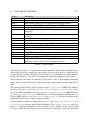
The Webots licenses comes in three different flavors, including Webots PRO, Webots EDU and
Webots MOD. They differ by the features and price. These different versions are described in
this section. The features available in the different versions are summarized in table 1.1.
1.1.1
Webots PRO
Webots PRO is the most powerful version of Webots. It is designed for research and development
projects. Webots PRO includes the possibility to create supervisor processes for controlling
robotics experiments, an extended physics programming capability and a fast simulation mode
(faster than real time). A 30 day trial version of Webots PRO is available from Cyberbotics web
site.
1.1.2
Webots EDU
Webots EDU is tailored for classrooms. Students learn how to model robots, create their own
environments and program the behavior of the robots, using any of the supported programming
languages. To validate their models, they can optionally transfer their control programs to real
robots. A 30 day trial version of Webots EDU is available upon request.
19
20
CHAPTER 1. INSTALLING WEBOTS
1.1.3
Webots MOD
Webots MOD is a special license mode in which the simulation software comes free of charge
and the users pay only for the modules they need. Various modules are available for purchase at
different price tags. They include special robot models (e.g., NAO, DARwIn-OP, e-puck, Thymio
2, etc.), object models (e.g., cardboard box, wooden box, etc.), environment models (e.g., robot
soccer field), programming libraries, programming languages (e.g., C/C++, Matlab, Python),
interfaces to third parties software or hardware, etc. They are all described on Cyberbotics web
site.
1.1.4
Webots licences overview
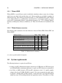
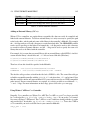
The following table summarizes the main differences between Webots PRO, Webots EDU and
Webots MOD.
Webots feature
Supervisor capability
Physics plug-in programming
Fast simulation mode
Robot and environment modelling
Robot programming
Transfer to real robots
Multi-platform: Windows, Mac & Linux
Floating licenses
One year Premier Service included
PRO
yes
yes
yes
yes
yes
yes
yes
yes
yes
EDU
no
no
no
yes
yes
yes
yes
yes
yes
MOD
no
no
no
no
yes/no (1)
yes/no (1)
yes
yes
yes
Table 1.1: Webots licenses summary
(1): refer to specific module description.
1.2
System requirements
The following hardware is required to run Webots:
• A fairly recent PC or Macintosh computer with at least a 2 GHz dual core CPU clock speed
and 2 GB of RAM is a minimum requirement. A quad-core CPU is however recommended.
• An nVidia or AMD (formerly ATI) OpenGL (minimum version 2.1) capable graphics
adapter with at least 512 MB of RAM is required. We do not recommend any other graphics adapters, including Intel graphics adapters, as they often lack a good OpenGL support
which may cause 3D rendering problems and application crashes. Nevertheless, in some
1.3. VERIFYING YOUR GRAPHICS DRIVER INSTALLATION
21
cases, the installation of the latest Intel graphics driver can fix such problems and let you
use Webots. However, we don’t provide any guarantee on this. For Linux systems, we recommend only nVidia graphics cards. Webots works well on all the graphics cards included
in fairly recent Apple computers. It is strongly advised to try the 30 day trial version of
Webots on your computer systems to ensure they are compatible before you buy.
The following operating systems are supported:
• Linux: Webots is ensured to run on the latest Ubuntu Long Term Support (LTS) release,
currently version 14.04. But it is also known to run on most recent major Linux distributions, including RedHat, Mandrake, Debian, Gentoo, SuSE, and Slackware. We recommend using a recent version of Linux. Webots is provided for Linux 64 (x86-64) systems.
Since Webots 8.1.0, the Linux 32 (i386) version is no longer provided. Webots doesn’t run
on Ubuntu version eariler than 12.04.
• Windows: Webots runs on Windows 10 64-bit, Windows 8.1 64-bit, Windows 8 64-bit and
Windows 7 64-bit. It is not supported on 32-bit versions of Windows and on old versions
including Windows Vista, XP, NT4 or 2000.
• Macintosh: Webots runs on Mac OS X 10.11 ”El Captan” and 10.10 ”Yosemite”. Webots
may work but is not officially supported on earlier versions of Mac OS X. Since version
6.3.0, Webots is compiled exclusively for Intel Macs, it does not run on old PowerPC
Macs. To use Webots on a PowerPC Mac, you need Webots 6.2.4 (or earlier), these older
versions were compiled as Universal Binary.
Other versions of Webots for other UNIX systems (Solaris, Linux PPC, Irix) may be available
upon request.
1.3
1.3.1
Verifying your graphics driver installation
Supported graphics cards
Webots officially supports only recent nVidia and ATI graphics adapters. So it is recommended to
run Webots on computers equipped with such graphics adapters and up-to-date drivers provided
by the card manufacturer (i.e., nVidia or ATI). Such drivers are often bundled with the operating
system (Windows, Linux and Mac OS X), but in some case, it may be necessary to fetch it from
the web site of the card manufacturer.
1.3.2
Unsupported graphics cards
Webots may nevertheless work with other graphics adapters, in particular the Intel graphics
adapters. However this is unsupported and may work or not, without any guarantee. Some
22
CHAPTER 1. INSTALLING WEBOTS
users reported success with some Intel graphics cards after installing the latest version of the
driver. Graphics drivers from Intel may be obtained from the Intel download center web site1 .
Linux graphics drivers from Intel may be obtained from the Intel Linux Graphics web site2 .
If some graphical bugs subsist, changing the ”RTT prefered mode” from the Webots OpenGL
Preferences from ”Framebuffer Object” to ”Pixelbuffer Object” or ”Direct Copy” may fix the
problems. However, this may also impact the 3D performance.
1.3.3
Upgrading your graphics driver
On Linux and Windows, you should make sure that the latest graphics driver is installed. On
the Mac the latest graphics driver are automatically installed by the Software Update, so Mac
users are not concerned by this section. Note that Webots can run up to 10x slower without
appropriate driver. Updating your driver may also solve various problems, i.e., odd graphics
rendering or Webots crashes.
Linux
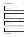
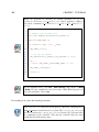
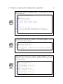
On Linux, use this command to check if a hardware accelerated driver is installed:
$ glxinfo | grep OpenGL
If the output contains the string ”NVIDIA”, ”ATI”, or ”Intel”, this indicates that a hardware
driver is currently installed:
$ glxinfo | grep OpenGL
OpenGL vendor string: NVIDIA Corporation
OpenGL renderer string: GeForce 8500 GT/PCI/SSE2
OpenGL version string: 3.0.0 NVIDIA 180.44
...
If you read ”Mesa”, ”Software Rasterizer” or ”GDI Generic”, this indicates that the hardware
driver is currently not installed and that your computer is currently using a slow software emulation of OpenGL:
$ glxinfo | grep OpenGL
OpenGL vendor string: Mesa project: www.mesa3d.org
OpenGL renderer string: Mesa GLX Indirect
OpenGL version string: 1.4 (1.5 Mesa 6.5.2)
...
In this case you should definitely install the hardware driver.
On Ubuntu the driver can usually be installed automatically from the Additional Drivers tab of
the Software & Update window. Otherwise you can find out what graphics hardware is installed
on your computer by using this command:
1
2
http://downloadcenter.intel.com
http://intellinuxgraphics.org
1.3. VERIFYING YOUR GRAPHICS DRIVER INSTALLATION
23
$ lspci | grep VGA
01:00.0 VGA compatible controller: nVidia Corporation GeForce 8500 GT
(rev a1)
Then you can normally download the appropriate driver from the graphics hardware manufacturer’s website: http://www.nvidia.com3 for an nVidia card or http://www.amd.com4 for a ATI
graphics card. Please follow the manufacturer’s instructions for the installation.
Windows
1. Right-click on My Computer.
2. Select Properties.
3. Click on the Device Manager tab.
4. Click on the plus sign to the left of Display adapters. The name of the driver appears. Make a note of it.
5. Go to the web site of your card manufacturer: http://www.nvidia.com5 for an nVidia card
or http://www.amd.com6 for a ATI graphics card.
6. Download the driver corresponding to your graphics card.
7. Follow the instructions from the manufacturer to install the driver.
1.3.4
Hardware acceleration tips
Linux
Depending on the graphics hardware, there may be a huge performance drop of the rendering
system (up to 10x) when compiz desktop effects are on. Also these visual effects may cause some
display bug where the main window of Webots is not properly refreshed. Hence, on Ubuntu (or
other Linux) we recommend to deactivate the desktop effects. You can easily disable them using
some tools like Compiz Config Settings Manager or Unity Twerk Tool.
3
http://www.nvidia.com
http://www.amd.com
5
http://www.nvidia.com
6
http://www.amd.com
4
24
CHAPTER 1. INSTALLING WEBOTS
1.4
Installation procedure
Usually, you will need to be ”administrator” to install Webots. Once installed, Webots can be
used by a regular, unprivileged user. To install Webots, please follow this procedure:
1. Uninstall completely any old version of Webots that may have been installed on your
computer previously.
2. Install Webots for your operating system as explained below.
After installation, the most important Webots features will be available, but
some third party tools (such as Java, Python, or MATLABTM ) may be necessary for running or compiling specific projects. The chapter 4 covers the set
up of these tools.
1.4.1
Linux
Webots will run on most recent Linux distributions running glibc2.11.1 or earlier. This includes
fairly recent Ubuntu, Debian, Fedora, SuSE, RedHat, etc. Webots comes in two different package
types: .deb and .tar.bz2 (tarball). The .deb package is aimed at the latest Ubuntu Linux
distribution whereas the tarball package includes many dependency libraries and there is therefore best suited for installation on other Linux distributions. These packages can be downloaded
from our web site7 .
Some of the following commands requires the root privileges. You can get
these privileges by preceding all the commands by the sudo command.
Webots will run much faster if you install an accelerated OpenGL drivers. If
you have a nVidia or ATI graphics card, it is highly recommended that you
install the Linux graphics drivers from these manufacturers to take the full
advantage of the OpenGL hardware acceleration with Webots. Please find
instructions here section 1.3.
Webots needs the avconv program to create MPEG-4 movies, that can be
installed with libav-tools and libavcodec-extra-54 packages.
7
http://www.cyberbotics.com/linux
1.4. INSTALLATION PROCEDURE
25
Using Advanced Packaging Tool (APT)
The advantage of this solution is that Webots will be updated with the system updates. This
installation requires the root privileges.
First of all, you may want to configure your apt package manager by adding this line:
deb http://www.cyberbotics.com/debian/ binary-i386/
or
deb http://www.cyberbotics.com/debian/ binary-amd64/
in the /etc/apt/sources.list configuration file. Then update the APT packages by using
apt-get update
Optionally, Webots can be autentified thanks to the Cyberbotics.asc signature file which
can be downloaded here8 , using this command:
apt-key add /path/to/Cyberbotics.asc
Then proceed to the installation of Webots using:
apt-get install webots
This procedure can also be done using any APT front-end tool such as the
Synaptic Package Manager. But only a command line procedure is documented here.
From the tarball package
This section explains how to install Webots from the tarball package (having the .tar.bz2
extension). This package can be installed without the root privileges. It can be uncompressed
anywhere using the tar xjf command line. Once uncompressed, it is recommended to set
the WEBOTS HOME environment variable to point to the webots directory obtained from the
uncompression of the tarball:
tar xjf webots-8.3.2-i386.tar.bz2
or
tar xjf webots-8.3.2-x86-64.tar.bz2
and
export WEBOTS_HOME=/home/username/webots
8
http://www.cyberbotics.com/linux
26
CHAPTER 1. INSTALLING WEBOTS
The export line should however be included in a configuration script like /etc/profile, so
that it is set properly for every session.
Some additional libraries are needed in order to properly run Webots. In particular libjpeg62,
libav-tools, libpci and libavcodec-extra-54 have to be installed on the system.
From the DEB package
This procedure explains how to install Webots from the DEB package (having the .deb extension).
On Ubuntu, double-click on the DEB package file to open it with the Ubuntu Software Center
and click on the Install button. If a previous version of Webots is already installed, then the text
on the button could be different, like Upgrade or Reinstall.
Alternatively, the DEB package can also be installed using dpkg or gdebi with the root
privileges. For 32-bit systems:
dpkg -i webots_8.3.2_i386.deb
apt-get -f install
or
gdebi webots_8.3.2_i386.deb
For 64-bit systems:
dpkg -i webots_8.3.2_amd64.deb
apt-get -f install
or
gdebi webots_8.3.2_amd64.deb
1.4.2
Windows
1. Download the webots-8.3.2_setup.exe installation file from our web site9 .
2. Double click on this file.
3. Follow the installation instructions.
It is possible to install Webots silently from an administrator DOS console, by typing webots-8.
3.2_setup.exe/SILENT or webots-8.3.2_setup.exe/VERYSILENT
If you observe 3D rendering anomalies or Webots crashes, it is strongly recommend to upgrade
your graphics driver.
9
http://www.cyberbotics.com/windows
1.5. WEBOTS LICENSE SYSTEM
1.4.3
27
Mac OS X
1. Download the webots-8.3.2.dmg installation file from our web site10 .
2. Double click on this file. This will mount on the desktop a volume named Webots containing the Webots folder.
3. Move this folder to your /Applications folder or wherever you would like to install
Webots.
1.5
Webots license system
Starting with Webots 8, a new license system was introduced to facilitate the use of Webots,
which replaces the previous system. Webots licenses can now be set-up on an unlimited number
of computers, allowing you to use Webots seamlessly on any computer (office, home, travel, etc.).
This new system relies on a license server located on Cyberbotics servers and accessible through
an Internet connection. If you would like to use Webots while not connected to the Internet, you
can transfer your Internet license from the server to your local computer for a limited duration.
After the expiration of this duration, your license will be automatically transferred back to the
license server.
Cyberbotics license servers are located in Switzerland on a highly reliable
network featuring a 99.9% up-time. However, if for some reason our servers
would fail, a security system will allow you to run Webots even in case of
server failure, by connecting automatically to an alternate server located in
the Cloud (hosted on Google App Engine).
1.5.1
Firewall configuration (optional)
If you plan to use Webots behind an Internet firewall, you should create two new rules in your
firewall configuration to allow connections to the following servers:
• https://www.cyberbotics.com (port 443)
• https://webots-license.appspot.com (port 443)
If you are using a proxy to access the Internet, Webots will retrieve your
system proxy configuration automatically.
10
http://www.cyberbotics.com/macosx
28
CHAPTER 1. INSTALLING WEBOTS
1.5.2
License agreement
Please read your license agreement carefully before using Webots. This license is provided
within the software package. By using the software and documentation, you agree to abide by
all the provisions of this license.
1.5.3
License setup
A Webots license is originally associated with an e-mail address which corresponds to a user
account on Cyberbotics’s web site.
When Webots is started for the first time, a login dialog invites you to register a user account on
Cyberbotics’s web site (if not already done) and to enter the corresponding license information
to log in your Webots session.
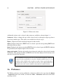
The Synchronization field of the Webots login dialog defines how frequently
Webots checks the license server. Setting this field to a small value will cause
more networking activity, but will allow you to release the license quickly
after a crash. This will allow you in turn to restart Webots quicker on another
machine. For example, if you select 5 minutes, you may have to wait for up
to 5 minutes if you crashed Webots on a machine and want to restart it on
another.
1.5.4
License administration
If you are the administrator of the license, you can log into your Webots account on Cyberbotics’
web site and go to the Administration page under the My Account tab. From there, you will be
able to monitor your licenses, to purchase more licenses, to create groups of users and to grant
customized user access to your licenses.
1.5.5
Module download folder
By default, Webots will download the different modules you purchased and store them in the
local user application folder:
• Windows: C:\Users\MyName\AppData\Local\Cyberbotics\Webots\8.0
• Mac OS X: /Users/MyName/Library/ApplicationSupport/Cyberbotics/
Webots/8.0
• Linux: /home/MyName/.local/share/Cyberbotics/Webots/8.0
1.6. CLASSROOM LICENSE SETUP
29
You may want to change this behavior and have Webots storing its module files in a different
folder. This is possible by setting the WEBOTS MODULES PATH environment variable to point
to a folder where the modules files will be downloaded and stored. It can be useful to do so
if you want to avoid that each user has its own copy of the module files. In such a case, it
is recommended for the users to start Webots with the --disable-modules-download
option to avoid overwritting files in this folder.
If you need further information about license issues, please send an e-mail to:
<[email protected]>
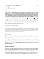
1.6
Classroom license setup
This section explains how to setup your Webots licenses to grant access to students in a classroom. It also explains how to manage student access to Webots licenses for homework Webots
exercices or projects. Let’s assume you purchased 20 licenses of Webots EDU and want to let
some of your students use them. You should ensure that your classroom machines can access the
Internet and in particular the license server of Cyberbotics11 . If it doesn’t work, you may need to
configure your local firewall to allow Webots to access this URL.
1.6.1
User account
There are two methods to handle student access to Webots licenses: a single user account, or
multiple user accounts.
Single user account
The single user account method is simpler to setup as you don’t need to know the e-mail addresses of the students. Nevertheless, you need to setup an e-mail address for a generic user for
which you can read the e-mails received. It could be your own personal e-mail address. Let’s
call this e-mail address [email protected]. A drawback to this method is that
it allows a single student to use simultaneously several instances of your 20 licenses, possibly all
of them, thus preventing other students to use them.
1. Log in to your Webots user account using your license administration credentials, e.g., the
user account which was used to activate your Webots licenses.
2. Create a new user pack from the administration page and call it ”Students”.
3. Grant access to all your 20 Webots EDU license (tick boxes).
11
https://www.cyberbotics.com/license
30
CHAPTER 1. INSTALLING WEBOTS
4. Set the concurrency value to 20 to allow the single user account to use all the licenses
simultaneously.
5. Type [email protected] in the ”users:” text area.
6. If the account doesn’t already exists, [email protected] will receive an
e-mail asking to create a user account at Cyberbotics’ web site12 .
7. Create this account (if needed), log in and visit the Profile page of this account. Copy the
”Alternate password for Webots 8”. This password allows students to use Webots, but not
to log in this user account. It looks like J6ebgAGRgFtkf8QHiWoHXIUnI98=.
8. Give this e-mail address and alternate password to your students to allow them to log in
Webots using your licenses (but they won’t be able to log in the web page).
Multiple user accounts
The multiple user accounts license requires that you have the list of e-mail addresses of the
students to whom you want to grant access to your Webots licenses. You will be able to limit
the number of simultaneous instances of Webots used per student to 1, so that a single student
cannot use multiple licenses simultaneously. Hence a single student cannot prevent the others
from using Webots.
1. Log in to your Webots user account using your license administration credentials, e.g., the
user account which was used to activate your Webots licenses.
2. Create a new user pack from the administration page and call it ”Students”.
3. Grant access to all your 20 Webots EDU license (tick boxes).
4. Set the concurrency value to 1 to prevent a single user to use multiple instances of Webots
at the same time.
5. Type (or copy/paste) the list of student e-mail addresses in the ”users:” text area.
6. Press the apply button. The e-mail addresses which are not already registered on Cyberbotics’ web site will receive an invitation e-mail explaining how to register a Webots
account and use the newly granted Webots licenses. For existing accounts, no e-mail is
sent and it is your responsibility to inform the students about their modified license rights.
12
https://www.cyberbotics.com
1.6. CLASSROOM LICENSE SETUP
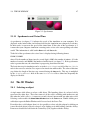
1.6.2
31
Classrom
Setup
You can install Webots on all the computers in a classroom, even if you have more computers
than licenses. In our example, if you have 20 licenses and 30 computers, then 20 students could
use the software simultaneously on any of the 30 computers. If a 21rst student comes in, he
won’t be able to start Webots until one of the 20 students stops using Webots.
Restrict the license to specific machines
It is possible to restrict the use of your licenses to a specific classroom, or more generally, to
a number of specific computers. This can be achieved from the ”Module pack” section of the
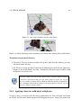
administration web page: click on the license you want to restrict and a new page entitled ”Edit
module pack” should be displayed. On this page, set an IP range value to limit the use of this
pack to machines with a specific IP address. For example: ”128.179.67.143, 128.179.67.146,
123.179.67.145” will limit the use of Webots to these 3 IP addresses. It is also possible to use an
IP mask (CIDR notation) to specify a range of IP addresses. For example, ”128.179.67.143/24,
128.178.12.122” will limit the use of Webots to any machine whose IP address starts with
128.179.67 and also to the machine whose IP address is 128.178.12.122. Machines that do
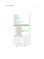
not match the values provided in the IP range field won’t be able to access the licenses.
Making things even simpler for students
To save the students from having to type an e-mail address and password on the first run of Webots, you may want to do it for them before the class starts. If you do it from the user account
they are supposed to use, this information will be saved and the students won’t need to enter it
again. You may also automate this process by copying an already configured Webots preferences
to all the user accounts used by the students. On Windows, the Webots preferences are stored in
the registry under the HKEY_CURRENT_USER/SOFTWARE/Cyberbotics key (so you need
to use a tool that copies registry keys across user accounts). On Mac OS X, the Webots preferences are stored in a file under the user home directory at ˜/Library/Preferences/com.
cyberbotics.Webots8.3.2.plist. On Linux, the Webots preferences are stored in a
file under the user home directory at ˜/.config/Cyberbotics/Webots8.3.2.conf.
1.6.3
Homework
If no IP restriction is set (see above), then the students will be able to use Webots anytime,
from any computer, including their own personal computers. In such a case, it’s better to use
multiple user accounts rather than a single one, to avoid that a few students use all the licenses
permanently.
32
1.6.4
CHAPTER 1. INSTALLING WEBOTS
Using Webots without Internet connection
It is possible to use Webots without any Internet connection for a limited amount of time. Users
who anticipate they will be away from the Internet can download a license locally on their machine for a specified lease duration. During this period of time, the license is considered to be
in use and is not available to other users. The maximum lease duration can be defined by the
administrator of the licenses in the ”Edit module pack” administration web page. It can be set
to ”None” to prevent any off-line use of Webots. Otherwise, the maximum lease value can be
chosen between 1 hour and 7 days.
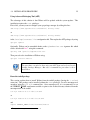
In order to download a license locally for off-line use, a user should go to the Tools menu of
Webots and open the License Manager... item. A new window should pop-up to display the
available licenses. The user can then choose which licenses to download on his local computer
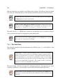
as well as the duration of the lease for these licenses. Warning: this operation cannot be undone.
Once transferred locally, the licenses are not available to other computers for the duration of the
lease period.
1.7
Translating Webots to your own language
Webots is translated into French, German, Spanish, Chinese and Japanese (and partially into
Italian). However, since Webots is always evolving, including new text or changing existing
wording, these translations may not always be complete or accurate. As a user of Webots, you
are very welcome to help us fix these incomplete or inaccurate translations. This is actually a
very easy process which merely consists of editing a UTF-8 XML file, and processing it with a
small utility. Your contribution is likely to be integrated into the upcoming releases of Webots,
and your name acknowledged in this user guide.
Even if your language doesn’t appear in the current Webots Preferences panel, under the General
tab, you can very easily add it. To proceed with the creation of a new translation or the improvement of an existing one, please follow the instructions located in the readme.txt file in the
Webots/resources/translations folder. Don’t forget to send us your translation files!
Chapter 2
Getting Started with Webots
This chapter gives an overview of Webots windows and menus.
2.1
2.1.1
Introduction to Webots
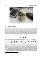
What is Webots?
Webots is a professional mobile robot simulation software package. It offers a rapid prototyping environment, that allows the user to create 3D virtual worlds with physics properties such
as mass, joints, friction coefficients, etc. The user can add simple passive objects or active objects called mobile robots. These robots can have different locomotion schemes (wheeled robots,
legged robots, or flying robots). Moreover, they may be equipped with a number of sensor and
actuator devices, such as distance sensors, drive wheels, cameras, motors, touch sensors, emitters, receivers, etc. Finally, the user can program each robot individually to exhibit the desired
behavior. Webots contains a large number of robot models and controller program examples to
help users get started.
Webots also contains a number of interfaces to real mobile robots, so that once your simulated
robot behaves as expected, you can transfer its control program to a real robot like e-puck,
DARwIn-OP, Nao, etc. Adding new interfaces is possible through the related sytem.
2.1.2
What can I do with Webots?
Webots is well suited for research and educational projects related to mobile robotics. Many
mobile robotics projects have relied on Webots for years in the following areas:
• Mobile robot prototyping (academic research, the automotive industry, aeronautics, the
vacuum cleaner industry, the toy industry, hobbyists, etc.)
33
34
CHAPTER 2. GETTING STARTED WITH WEBOTS
• Robot locomotion research (legged, humanoids, quadrupeds robots, etc.)
• Multi-agent research (swarm intelligence, collaborative mobile robots groups, etc.)
• Adaptive behavior research (genetic algorithm, neural networks, AI, etc.).
• Teaching robotics (robotics lectures, C/C++/Java/Python programming lectures, etc.)
• Robot contests (e.g. www.robotstadium.org1 or www.ratslife.org2 )
2.1.3
What do I need to know to use Webots?
You will need a minimal amount of technical knowledge to develop your own simulations:
• A basic knowledge of the C, C++, Java, Python or Matlab programming language is necessary to program your own robot controllers. However, even if you don’t know these
languages, you can still program the e-puck and Hemisson robots using a simple graphical
programming language called BotStudio.
• If you don’t want to use existing robot models provided within Webots and would like to
create your own robot models, or add special objects in the simulated environments, you
will need a basic knowledge of 3D computer graphics and VRML97 description language.
That will allow you to create 3D models in Webots or import them from 3D modelling
software.
2.1.4
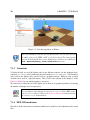
Webots simulation
A Webots simulation is composed of following items:
1. A Webots world file (.wbt) that defines one or several robots and their environment. The
.wbt file does sometimes depend on external PROTO files (.proto) and textures.
2. One or several controller programs for the above robots (in C/C++/Java/Python/Matlab).
3. An optional physics plugin that can be used to modify Webots regular physics behavior (in
C/C++).
1
2
http://www.robotstadium.org
http://www.ratslife.org
2.1. INTRODUCTION TO WEBOTS
2.1.5
35
What is a world?
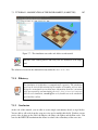
A world, in Webots, is a 3D description of the properties of robots and of their environment.
It contains a description of every object: position, orientation, geometry, appearance (like color
or brightness), physical properties, type of object, etc. Worlds are organized as hierarchical
structures where objects can contain other objects (like in VRML97). For example, a robot can
contain two wheels, a distance sensor and a joint which itself contains a camera, etc. A world
file doesn’t contain the controller code of the robots; it only specifies the name of the controller
that is required for each robot. Worlds are saved in .wbt files. The .wbt files are stored in the
worlds subdirectory of each Webots project.
2.1.6
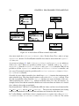
What is a controller?
A controller is a computer program that controls a robot specified in a world file. Controllers
can be written in any of the programming languages supported by Webots: C, C++, Java, Python
or MATLABTM . When a simulation starts, Webots launches the specified controllers, each as a
separate process, and it associates the controller processes with the simulated robots. Note that
several robots can use the same controller code, however a distinct process will be launched for
each robot.
Some programming languages need to be compiled (C and C++) other languages need to be
interpreted (Python and MATLABTM ) and some need to be both compiled and interpreted (Java).
For example, C and C++ controllers are compiled to platform-dependent binary executables
(for example .exe under Windows). Python and MATLABTM controllers are interpreted by the
corresponding run-time systems (which must be installed). Java controller need to be compiled
to byte code (.class files or .jar) and then interpreted by a Java Virtual Machine.
The source files and binary files of each controller are stored together in a controller directory. A
controller directory is placed in the controllers subdirectory of each Webots project.
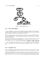
2.1.7
What is a Supervisor?
The Supervisor is a privileged type of Robot that can execute operations that can normally only
be carried out by a human operator and not by a real robot. The Supervisor is normally associated
with a controller program that can also be written in any of the above mentioned programming
languages. However in contrast with a regular Robot controller, the Supervisor controller will
have access to privileged operations. The privileged operations include simulation control, for
example, moving the robots to a random position, making a video capture of the simulation, etc.
36
2.2
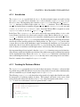
CHAPTER 2. GETTING STARTED WITH WEBOTS
Starting Webots
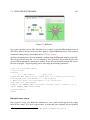
The first time you start Webots it will open the ”Welcome to Webots!” menu with a list of possible
starting points.
2.2.1
Linux
Open a terminal and type webots to launch Webots.
2.2.2
Mac OS X
Open the directory in which you installed the Webots package and double-click on the Webots
icon.
2.2.3
Windows
On Windows 10 and Windows 7, open the Start menu, go to the Program Files > Cyberbotics
menu and click on the Webots 8.3.2 menu item.
On Windows 8, open the Start screen, scroll to the screen’s right until spotting the Cyberbotics
section and click on the Webots icon.
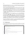
2.2.4
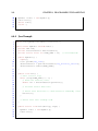
Command Line Arguments
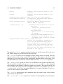
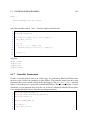
Following command line options are available when starting Webots from a Terminal (Linux/Mac) or a Command Prompt (Windows):
SYNOPSIS: webots [options] [worldfile]
OPTIONS:
--minimize
minimize Webots window on startup
--mode=<mode>
choose startup mode (overrides
application preferences)
argument <mode> must be one of:
pause, realtime, run or fast
(Webots PRO is required to use:
--mode==run or --mode=fast)
--help
display this help message and exit
--sysinfo
display information of the system and
exit
--version
display version information and exit
--uuid
display the UUID of the computer and
exit
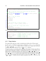
2.2. STARTING WEBOTS
37
--stdout
redirect the controller stdout to the
terminal
--stderr
redirect the controller stderr to the
terminal
--disable-modules-download skip the check for module updates
--force-modules-download
automatically download module updates
(if any) at startup
--start-streaming-server
starts the Webots streaming server
(Webots PRO is required)
[="key[=value];..."]
parameters may be given as an option:
port=1234 :
starts the streaming server
on port 1234
monitorActivity :
prints a dot ’.’ on stdout every
5 seconds
disableStandardStreamsRedirection :
disables the streaming of the
standard output and error streams
--log-performance="<file path>[,<steps count>]"
measure the performance of Webots and
log it in the specified <file path>
file. <steps count> is an optional
integer value that specifies how many
steps are analyzed. If ’--sysinfo’ is
also set then the system information are
printed in the log file.
The optional worldfile argument specifies the name of a .wbt file to open. If it is not specified, Webots attempts to open the most recently opened file.
The --minimize option is used to minimize (iconize) Webots window on startup. This also
skips the splash screen and the eventual Welcome Dialog. This option can be used to avoid
cluttering the screen with windows when automatically launching Webots from scripts. Note
that Webots PRO does automatically enable the Fast mode when --minimize is specified.
The --mode=<mode> option can be used to start Webots in the specified execution mode.
The four possible execution modes are: pause, realtime, run and fast; they correspond
to the simulation control buttons of Webots’ graphical user interface. This option overrides, but
does not modify, the startup mode saved in Webots’ preferences. For example, type webots
--mode=pause filename.wbt to start Webots in pause mode. Note that run and fast
modes are only available in Webots PRO.
The --sysinfo option displays misc information about the current system on the standard
output stream and quits Webots.
The --stdout and --stderr options have the effect of redirecting Webots console output to
38
CHAPTER 2. GETTING STARTED WITH WEBOTS
the calling terminal or process. For example, this can be used to redirect the controllers output to
a file or to pipe it to a shell command. --stdout redirects the stdout stream of the controllers,
while --stderr redirects the stderr stream. Note that the stderr stream may also contain
Webots error or warning messages.
The --disable-modules-download option disables the download of new modules and
therefore prevents the Webots Update Manager window from poping up. The --forcemodules-download will instead force the automatic download of new modules (if available)
without asking the user. Both options are mutually exclusive.
The --start-streaming-server option starts the Webots streaming server. An option
can be given to change the default parameters of the streaming server. This option is a string
containing a list of parameter keys and their values separated by semicolons. The supported
options are described in table 2.1.
Key
port
Value example
1234
Description
The port on which the streaming server is open
Table 2.1: Streaming server options
For example, the following command will start Webots with the streaming server enabled on the
TCP port ’1234’: webots --start-streaming-server="port:1234"
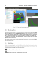
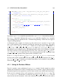
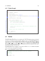
2.3
The User Interface
Webots GUI is composed of four principal windows: the 3D window that displays and allows
to interact with the 3D simulation, the Scene tree which is a hierarchical representation of the
current world, the Text editor that allows to edit source code, and finally, the Console that displays
both compilation and controller outputs.
The GUI has nine menus: File, Edit, View, Simulation, Build, Robot, Tools, Wizards and Help.
2.3.1
File Menu
The File menu allows you to perform usual file operations: loading, saving, etc.
The New World menu item (and button) opens a new world in the simulation window containing
only an ElevationGrid, displayed as a chessboard of 10 x 10 squares on a surface of 1 m x
1 m.
The Open World... menu item (and button) opens a file selection dialog that allows you to
choose a .wbt file to load.
2.3. THE USER INTERFACE
39
Figure 2.1: Webots GUI
The Open Recent World menu item gives the possibility of reopening a .wbt file that was opened
recently by choosing it from the list displayed in the submenu.
The Open Sample World menu item opens a dialog listing all the available sample worlds where
it is possible to search for a specific .wbt file to load by entering the file name or part of it in
the search field.
The Save World menu item (and button) saves the current world using the current filename
(the filename that appears at the top of the main window). On each Save the content of the .wbt
file is overwritten and no backup copies are created by Webots, therefore you should use this
button carefully and eventually do safety copies manually.
The Save World As... menu item (and button) saves the current world with a new filename entered
by the user. Note that a .wbt file should always be saved in a Webots project directory, and in
the worlds subdirectory, otherwise it will not be possible to reopen the file.
The Revert World menu item (and button) reloads the current world from the saved version
and restarts the simulation from the beginning.
40
CHAPTER 2. GETTING STARTED WITH WEBOTS
When opening (or reverting) a world, if the world takes more than 2 seconds
to load a window will pop up and show the progression. Using this window
it is possible to cancel the loading of the world, in that case, the empty world
will be opened instead.
The New Text File menu item (and button) opens an empty text file in the text editor.
The Open Text File... menu item (and button) opens a file selection dialog that allows you
to choose a text file (for example a .java file) to load.
The Save Text File menu item (and button) saves the current text file.
The Save Text File As... menu item (and button) saves the current text file with a new
filename entered by the user.
The Save All Text Files menu item saves all the opened and unsaved text files.
The Revert Text File menu item (and button) reloads the text file from the saved version.
The Print Preview... menu item opens a window allowing you to manage the page layout in order
to print files from the text editor.
The Print... menu item opens a window allowing you to print the current file of the text editor.
The Import VRML 2.0... menu item adds VRML97 objects at the end of the scene tree. These
objects come from a VRML97 file you must specify. This feature is useful for importing complex
shapes that were modeled in a 3D modelling program, then exported to VRML97 (or VRML 2.0).
Most 3D modelling software, like 3D Studio Max, Maya, AutoCAD, Pro Engineer, AC3D, or Art
Of Illusion, include the VRML97 (or VRML 2.0) export feature. Be aware that Webots cannot
import files in VRML 1.0 format. Once imported, these objects appear as Group, Transform
or Shape nodes at the bottom of the scene tree. You can then either turn these objects into
Webots nodes (like Solid, DifferentialWheels, etc.) or cut and paste them into the
children list of existing Webots nodes.
The Export VRML 2.0... item allows you to save the currently loaded world as a .wrl file,
conforming to the VRML97 standard. Such a file can, in turn, be opened with any VRML97
viewer and most 3D modeling software.
The Take Screenshot... item allows you to take a screenshot of the current view in Webots.
It opens a file dialog to save the current view as a PNG or JPG image.
2.3. THE USER INTERFACE
41
The Make Movie... item allows you to create MPEG movies (Linux and Mac OS X) or AVI
movies (Windows). Once the movie recording is started, this item is changed in Stop Movie....
During the recording, it is possible to the change the running mode and pause the simulation.
However, frames are only captured during Webots steps and not when the simulation is paused.
The Export HTML5 Model... item allows you to export the current world as an interactive 3D
.html file, using the X3DOM web standard, based on WebGL. This is especially useful for
publishing Webots-created worlds on the Web. X3DOM is supported in recent versions of Firefox, Chrome, Internet Explorer and Safari on Mac OS X (see details on the X3DOM web site3 ).
With the Chrome browser, in order to be able to open HTML/X3DOM files
locally, e.g., not from the Web, you may need to allow Chrome to open local files referred to by the HTML/X3DOM file, e.g., textures. This can be
achieved by passing the --allow-file-access-from-files option
at Chrome startup. Otherwise textures won’t show up in the 3D models.
The Make HTML5 Animation... item allows you to record a simulation as a 3D animation and
publish it on a HTML5 web page. The result is similar to a movie with playback controls, except
that you can change the viewpoint at any time. Several files are generated: an X3D file containing
the 3D scene, a JSON file containing the animation data and a HTML5 file displaying the result
using X3DOM and jQuery. Once the animation recording is started, this item is changed to Stop
HTML5 Animation... and can be used to stop the animation recording.
The Quit Webots terminates the current simulation and closes Webots.
2.3.2
Edit Menu
The Edit menu provides usual text edition functions to manipulate files opened in the Text editor,
such as Copy, Paste, Cut, etc.
2.3.3
View Menu
The View menu allows to control the viewing in the simulation window.
The Follow Object menu item allows to switch between a fixed (static) viewpoint and a viewpoint
that follows a mobile object (usually a robot). If you want the viewpoint to follow an object, first
you need to select the object with the mouse and then check the Follow Object menu item. Note
that the Follow Object state is saved in the .wbt file.
3
http://www.x3dom.org
42
CHAPTER 2. GETTING STARTED WITH WEBOTS
The Restore Viewpoint item restores the viewpoint’s position and orientation to their initial settings when the file was loaded or reverted. This feature is handy when you get lost while navigating in the scene, and want to return to the original viewpoint.
The Fullscreen item enables and disables displaying the 3D window on the entire screen.
The Projection radio button group allows to choose between the Perspective Projection (default)
and the Orthographic Projection mode for Webots simulation window. The perspective mode
corresponds to a natural projection: in which the farther an object is from the viewer, the smaller
it appears in the image. With the orthographic projection, the distance from the viewer does
not affect how large an object appears. Furthermore, with the orthographic mode, lines which
are parallel in the model are drawn parallel on the screen, therefore this projection is sometimes
useful during the modelling phase. No shadows are rendered in the orthographic mode.
The Rendering radio button group allows to choose between the Plain Rendering (default) and
the Wireframe modes for Webots simulation window. In plain rendering mode, the objects are
rendered with their geometrical faces, materials, colors and textures, in the same way they are
usually seen by an eye or a camera. In wireframe rendering mode, only the segments of the renderable primitives are rendered. This mode can be useful to debug your meshes. If the wireframe
rendering mode and the View > Optional Rendering > Show All Bounding Objects toggle button
are both activated, then only bounding objects are drawn (not the renderable primitives). This
can be used to debug a problem with the collision detection.
Finally, the Optional Rendering submenu allows to display, or to hide, supplementary information. These rendering are displayed only in the main rendering and hide in the robot camera.
They are used to understand better the behavior of the simulation.
The Show Coordinate System allows to display, or to hide, the global coordinate system at the
bottom right corner of the 3D window as red, green and blue arrows representing the x, y and z
axes respectively.
The Show All Bounding Objects allows to display, or to hide, all the bounding objects (defined in
the boundingObject fields of every Solid node). Bounding objects are represented by white lines.
These lines turn rose when a collision occurs and blue when the solid is idle, i.e., it comes to rest
and it doesn’t interact with any other active solid.
The Show Contact Points allows to display, or to hide, the contact points generated by the collision detection engine. Contact points that do not generate a corresponding contact force are not
shown. A contact force is generated only for objects simulated with physics (Physics node
required). A step is required for taking this operation into account.
The Show Connector axes allows to display, or to hide, the connector axes. The rotation alignments are depicted in black while the y and z axes respectively in green and blue.
The Show Joint axes allows to display, or to hide, the joint axes. The joint axes are represented
by black lines.
The Show Camera frustums allows to display, or to hide, the OpenGL culling frustum for every
camera in the scene, using a magenta wire frame. The OpenGL culling frustum is a truncated
2.3. THE USER INTERFACE
43
pyramid corresponding to the field of view of a camera. The back of the pyramid is not represented because the far plane is set to infinity. More information about this concept is available in
the OpenGL documentation.
The Show Distance Sensor rays allows to display, or to hide, the rays casted by the distance
sensor devices. These rays are drawn as red lines (which become green beyond collision points).
Their length corresponds to the maximum range of the device.
The Show Light Sensor rays allows to display, or to hide, the rays casted by the light sensor
devices. These rays are drawn as yellow lines.
The Show Lights allows to display, or to hide, the lights (including PointLights and SpotLights).
DirectionalLights aren’t represented. PointLights and SpotLights are represented by a colored
circle surrounded by a flare.
The Show Pen Painting Rays allows to display, or to hide, the rays in which the pen devices paint.
These rays are drawn as violet lines if painting is enabled, otherwise as gray lines.
The Show Center Of Mass and Support Polygon allows to display, or to hide, both the global
center of mass of a selected solid (with non NULL Physics node) and its support polygon. By
support polygon we mean the projection of the convex hull of the solid’s contact points on the
horizontal plane which contains the lowest one. In addition, the projection of the center of mass
in the latter plane is rendered in green if it lies inside the support polygon (static equilibrium),
red otherwise. This rendering option can be activated only for solids with no other solid at their
top.
If the Disable selection option is enabled, it prevents you from changing the selected solid node
when clicking on the 3D window. This is particularly useful during the modeling phase, when
you want to change the viewpoint without modifying the visible and selected fields in the scene
tree.
2.3.4
Simulation Menu
The Simulation menu is used to control the execution of the simulation.
The Pause menu item (and button) pauses the simulation.
The Step menu item (and button) executes one basic time step of simulation. The duration
of this step is defined in the basicTimeStep field of the WorldInfo node, and can be
adjusted in the scene tree window to suit your needs.
The Real-time menu item (and button) runs the simulation at real-time until it is interrupted
by Pause or Step. In run mode, the 3D display of the scene is refreshed every n basic time steps,
where n is defined in the displayRefresh field of the WorldInfo node.
44
CHAPTER 2. GETTING STARTED WITH WEBOTS
The Run menu item (and button) is like Real-time, except that it runs as fast as possible
(Webots PRO only).
The Fast menu item (and button) is like Run, except that no graphical rendering is performed (Webots PRO only). As the graphical rendering is disabled (black screen) this allows
for a faster simulation and therefore this is well suited for cpu-intensive simulations (genetic
algorithms, vision, learning, etc.).
2.3.5
Build Menu
The Build menu provides the functionality to compile (or cross-compile) controller code. The
build menu is described in more details here.
2.3.6
Robot Menu
The Robot menu provides actions specific to Robot nodes. Some actions of this menu are active
only when a robot is selected in the 3D window or when there is only one robot in the simulation:
The Edit Controller menu item opens the source file of the controller of the selected robot.
The Camera Devices submenu contains the list of all the camera devices of the selected robot
and lets the user show or hide single camera overlay images by checking or unchecking the
corresponding item. Camera overlays differ from the display overlays because of their magenta
border. Note that if the Hide All Camera Overlays item is checked, then the camera device overlays
will not be visible in the 3D view independently from the status of Camera Devices menu items.
A Camera Devices menu item is disabled if the overlay’s texture is shown in an external window
by double-clicking on it.
The Display Devices submenu contains the list of all the display devices of the selected robot
and lets the user show or hide single display overlay images by checking or unchecking the
corresponding item. Display overlays differ from the camera overlays because of their cyan
border. Note that if the Hide All Display Overlays item is checked, then the display device overlays
will not be visible in the 3D view independently from the status of Display Devices menu items.
A Display Devices menu item is disabled if the overlay’s texture is shown in an external window
by double-clicking on it.
On the other hand the following items are always active and apply to all the robot in the world:
The Hide All Camera Overlays option hides all the camera devices overlays in the 3D view independently from the specific robot’s device option set in Camera Devices submenu.
The Hide All Display Overlays option hides all the display devices overlays in the 3D view independently from the specific robot’s device option set in Display Devices submenu.
2.3. THE USER INTERFACE
2.3.7
45
Tools Menu
The Tools menu allows you to open various Webots windows.
The 3D View menu item shows or hides the
The Scene Tree menu item opens the
The Scene Tree menu item opens the Scene Tree window in which you can edit the virtual
world. Alternatively it is also possible to double-click on some of the objects in the main window:
this automatically opens the Scene Tree with the corresponding object selected.
The Text Editor menu item opens the Webots text editor. This editor can be used for editing and
compiling controller source code.
The Console menu item opens the Webots Console, which is a read-only console that is used to
display Webots error messages and controller outputs.
The Restore Layout menu item restores the factory layout of the panes of the main window.
The Clear Console menu item clears the console.
The Edit Physics Plugin menu item opens the source code of the physics plugin in the text editor.
The License Manager... item opens the Webots License Manager window that allows you to see
which license modules are in use and optionally to transfer some license modules to your local
computer for off-line use. Please note that the transfer of license modules may be limited by
your local license administrator: It may not be possible to transfer some modules to your local
computer or only for a limited duration depending on the configuration defined by your local
license administrator. Please ask your local license administrator in case of problem.
The Preferences item pops up a window described in this section.
2.3.8
Wizards Menu
The Wizards menu makes it easier to create new projects and new controllers.
The New Project Directory... menu item first prompts you to choose a filesystem location and
then it creates a project directory. A project directory contains several subdirectories that are
used to store the files related to a particular Webots project, i.e. world files, controller files, data
files, plugins, etc. Webots remembers the current project directory and automatically opens and
saves any type of file from the corresponding subdirectory of the current project directory.
The New Robot Controller... menu item allows you to create a new controller program. You will
first be prompted to choose between a C, C++, Java, Python or MATLABTM controller. Then,
Webots will ask you to enter the name of your controller and finally it will create all the necessary
files (including a template source code file) in your current project directory.
The New Physics Plugin... menu item will let you create a new physics plugin for your project.
Webots asks you to choose a programming language (C or C++) and a name for the new physics
plugin. Then it creates a directory, a template source code file and a Makefile in your current
project.
46
CHAPTER 2. GETTING STARTED WITH WEBOTS
2.3.9
Help menu
In the Help menu, the About... item opens the About... window that displays the license
information.
The Webots Guided Tour... menu item starts a guided tour that demonstrates Webots capabilies
through a series of examples.
The OpenGL Information... menu item gives you information about your current OpenGL hardware and driver. It can be used to diagnose rendering problems.
The remaining menu items bring up various information as indicated, in the form of HTML
pages, PDF documents, etc.
2.3.10
Main toolbar
The main toolbar contains items for editing the world and the speedometer (see subsection subsection 2.3.11), other than shortcuts to items of the File, Simulation and View menus. Edit actions
always apply on the selected object, that is highlighted both in the 3D window and in the Scene
Tree.
Hide/Show Scene Tree:
shows or hides the Scene Tree and resizes the 3D window conse-
quently.
Cut:
Cuts the selected object.
Copy:
Copies the selected object.
Paste:
Pastes the copied or cut object.
Note that the first three nodes of the Scene Tree (WorldInfo, Viewpoint, and Background) cannot be cut, copied or pasted. One single instance of each of these nodes must be
present in every Webots world, and in that precise order.
Add: Adds a node or an object. For nodes, this triggers a dialog that will let you choose
a node type from a list. The new node is created with default values that can be modified afterwards. You can only insert a node suitable for the corresponding field. The dialog also gives
the possibility to load a previously exported node by clicking on the Import... button. Further
information about how to export a node are available here.
Delete:
Deletes the selected object.
2.4. THE 3D WINDOW
47
Figure 2.2: Speedometer
2.3.11
Speedometer and Virtual Time
A speedometer (see figure 2.2) indicates the speed of the simulation on your computer. It is
displayed on the main toolbar, and indicates how fast the simulation runs compared to real time.
In other words, it represents the speed of the virtual time. If the value of the speedometer is 2,
it means that your computer simulation is running twice as fast as the corresponding real robots
would. This information is valid both in Run mode and Fast mode.
To the left of the speedometer, the virtual time is displayed using following format:
H:MM:SS:MMM
where H is the number of hours (may be several digits), MM is the number of minutes, SS is the
number of seconds, and MMM is the number of milliseconds (see figure 2.2). If the speedometer
value is greater than one, the virtual time is progressing faster than real time.
The basic time step for simulation can be set in the basicTimeStep field of the WorldInfo
node in the scene tree window. It is expressed in virtual time milliseconds. The value of this time
step defines the length of the time step executed during the Step mode. This step is multiplied
by the displayRefresh field of the same WorldInfo node to define how frequently the
display is refreshed.
2.4
The 3D Window
2.4.1
Selecting an object
A single mouse click allows to select a solid object. The bounding object of a selected solid is
represented by white lines. These lines turn rose if the solid is colliding with another one and
blue when the solid is idle, i.e., it comes to rest and it doesn’t interact with any other active solid.
Selecting a robot enables the Show Robot Window item in the Tools menu. Double-clicking on a
solid object opens the Robot Window and if it was closed, the Scene Tree.
If an object has a solid subpart, then it is also possible to select only this subpart by clicking on
it once the whole object is already selected, or by clicking on it while holding down the Alt key.
Linux users should also hold down the Control key (Ctrl) together with the Alt key.
48
CHAPTER 2. GETTING STARTED WITH WEBOTS
2.4.2
Navigation in the scene
Dragging the mouse while pressing a mouse button moves the camera of the 3D window.
• Camera rotation: In the 3D window, press the left button and drag the mouse to select an
object and rotate the viewpoint about it. If no object is selected, the camera rotates about
the origin of the world coordinate system.
• Camera translation: In the 3D window, press the right button and drag the mouse to translate the camera with the mouse motion.
• Zooming / Camera rotation: In the 3D window, press both left and right mouse buttons
simultaneously (or just the middle button) and drag the mouse vertically, to zoom in and
out. Dragging the mouse horizontally will rotate the camera about the viewing axis. Alternatively, the mouse wheel alone can also be used for zooming.
If you are a Mac user with a single button mouse, hold the Alt key and press
the mouse button to translate the camera according to the mouse motion.
Hold the control key (Ctrl) down and press the mouse button to zoom / rotate
the camera with the mouse motion.
2.4.3
Moving a solid object
Currently Webots provides two different ways to move solid objects: axis-aligned handles and
keyboard shortcuts.
Axis-aligned handles
When a solid object is selected, some arrow-shaped handles appear in the 3D window (see figure
2.3). These handles can be used to translate and rotate the object along the corresponding axis.
For moving the object you can simply click on the handle and drag it to the desired position.
A label will show the currect relative translation or rotation during the movement, as shown in
figure 2.4.
If the Control key (Ctrl), the handles for resizing the solid object will be displayed instead of
translation and rotation handles. These resize handles can also be enabled from the Field Editor.
2.4. THE 3D WINDOW
49
Figure 2.3: Axis-aligned handles to move solid objects
Figure 2.4: Labels displaying relative translation and rotation when moving objects with handles
Translation using keyboard shurtcuts
• Translation: To move an object parallel to the ground: hold down the shift key, press the
left mouse button and drag.
• Lift: To raise or lower and object: hold down the Shift key, press both left and right mouse
buttons (or the middle button) and drag. Alternatively, the mouse wheel combined with
the Shift key can also be used.
If you are a Mac user with a single button mouse, hold the Shift key and the
Control key (Ctrl) down and press the mouse button to rotate the selected
object according to mouse motion. Hold the Shift key and the Command key
(key with Apple symbol) down and press the mouse button to lift the selected
object according to mouse motion.
2.4.4
Applying a force to a solid object with physics
To apply a force to an object, place the mouse pointer where the force will apply, hold down
the Alt key and left mouse button together while dragging the mouse. Linux users should also
50
CHAPTER 2. GETTING STARTED WITH WEBOTS
hold down the Control key (Ctrl) together with the Alt key. This way your are drawing a 3Dvector whose end is located in the plane parallel to the view which passes through the point of
application. The intensity of the applied force is directly proportional to the cube of the length
of this vector.
2.4.5
Applying a torque to a solid object with physics
To apply a torque to an object, place the mouse pointer on it, hold down the Alt key and right
mouse button together while dragging the mouse. Linux users should also hold down the Control
key (Ctrl) together with the Alt key. Also, Mac OS X users with a one-button mouse should hold
down the Control key (Ctrl) to emulate the right mouse button. This way your are drawing a 3Dvector with origin the center of mass and whose end is located in the plane parallel to the view
which passes through this center. The object is prompted to turn around the vector direction,
the intensity of the applied torque being directly proportional to the product of the mass by the
length of the 3D-vector.
In pause mode, you can simultaneously add a force and a torque to the same
selected solid. Camera rotation can be useful when checking wether your
force / torque vector has the desired direction.
2.4.6
Moving and resizing Overlays
By default for each Camera and Display device, an overlay showing the recorded or displayed
image is visible in the 3D view. The device type is indicated by the border color: magenta for
Camera devices and cyan for Display devices, see figure 2.5. This overlay can be moved to the
desired position on the view by clicking on it and dragging the mouse. In order to resize the
overlay the user has to click on the icon located at the bottom right corner and drag the mouse,
during this action the original not scaled image size will be indicated using darker areas, as
depicted in figure 2.6 Additionally a close button is available on the top right corner to hide the
overlay. Once the robot is selected, it is also possible to show or hide the overlay images from
the Camera Devices and Display Devices items in Robot menu.
2.4.7
Show Camera and Display images in separate window
Overlay images can also be displayed outside the 3D window, see figure 2.7. When doubleclicking with the left mouse button on the overlay, a new external window displaying the device
image is created and the overlay in the 3D window is disabled. It is possible to restore the 3D
window overlay simply by closing the window.
2.4. THE 3D WINDOW
51
Figure 2.5: Camera and Display overlays
Figure 2.6: Camera overlay resizing
52
CHAPTER 2. GETTING STARTED WITH WEBOTS
Figure 2.7: Camera and Display image window
2.5
The Scene Tree
As seen in the previous section, to access to the Scene Tree Window you can either choose Scene
in the Tools menu, or press the Show Scene Tree button in the main toolbar. The scene tree
contains the information that describes a simulated world, including robots and environment,
and its graphical representation. The scene tree of Webots is structured like a VRML97 file. It
is composed of a list of nodes, each containing fields. Fields can contain values (text strings,
numerical values) or other nodes.
Tree
This section describes the user interface of the Scene Tree, gives an overview of the VRML97
nodes and Webots nodes.
2.5.1
Field Editor
Nodes can be expanded with a double-click. When a field is selected, its value can be edited at
the bottom of the Scene Tree. All changes will be immediately reflected in the 3D window. The
following buttons are available int the field editor section:
Reset:
Help:
Resets a field to its default value.
Context sensitive help for the currently selected node.
2.5. THE SCENE TREE
53
Figure 2.8: Scene Tree Window
54
CHAPTER 2. GETTING STARTED WITH WEBOTS
Figure 2.9: Webots node editor
Additionally, when a node is selected, other actions are available as shown in figure 2.9:
Tranform to:
Allow to change the type of the selected node by chosing the target type from a
given list of suitable types. This action is not available for all node’s types.
Export...:
Exports nodes that can then be imported in other worlds.
Source:
Displayed only when a PROTO node is selected, opens the corresponding PROTO definition file in the text editor.
Result:
Displayed only when a procedural PROTO node is selected, opens the PROTO definition
file generated by the template engine in the text editor.
Show resize handles: Displays the handles for resizing and scaling the selected node from the
3D Window. This option is disabled for PROTO nodes and only displayed for Geometry nodes
and nodes derived from Transform.
We recommend to use the Scene Tree to write Webots world files. However,
because the nodes and fields are stored in a human readable form, it is also
possible to edit world files with a regular text editor. Some search and replace
operations may actually be easier that way. Please refer to Webots Reference
Manual for more info on the available nodes and the world file format.
2.6
Preferences
The Webots preferences can be modified by a dialog box which can be open from the Webots
> Preferences menu item on Mac, and from the Tools > Preferences menu item on the other
operating systems.
2.6. PREFERENCES
55
The dialog box is separated into tabs. Each of the following subsection corresponds to one of
this tab.
2.6.1
General
The General tab contains misc preferences about the application.
• The Language option allows you to choose the language of Webots user interface (restart
needed).
• The Startup mode allows you to choose the state of the simulation when Webots is started
(pause, realtime, run, fast; see the Simulation menu).
• The Editor font defines the font to be used in Webots text editor and in the Console. It is
recommended to select a fixed width font for better source code display. The default value
of this preference is ”Consolas,10” on Windows, ”Courier,14” on Mac and ”Monospace”
on linux.
• The Number of threads defines how many threads can be created by Webots at maximum.
The recommended value matches with the number of logical cores of the computer processor. It may be interesting to reduce this value in some specific cases, for example when
another process requires intensively other cores. For now this value affects only the physical engine speed, and the controller compilation speed. Note that this is the maximum
number of threads allowed, but the actual number of threads used is the one defined in the
optimalThreadCount field of the WorldInfo node.
2.6.2
OpenGL
The OpenGL tab contains preferences about setting the 3D rendering abilities. The initial parameters of these settings may vary from one computer to another depending on the GPU OpenGL
abilities.
• The RTT preferred mode option allows you to modify the method used to create the Camera
device images. The methods are sorted from the most efficient one to the less efficient one.
• The Disable shadows option allows you to disable completely the shadows in the 3D view
and in the Camera rendering, whatever the values of the Light.castShadows fields.
The global performances can be improved by disabling this feature, but on the other hand
the rendering is more difficult to understand, and less pretty.
• The Disable shader option allows you to use the regular OpenGL shading model, instead
of a custom shading. This custom shading model computes the light effects on the 3D
objects per pixel instead of per vertex, resulting in a much smoother rendering. It may be
interesting to disbale this feature on old GPU if the shaders are not well supported.
56
CHAPTER 2. GETTING STARTED WITH WEBOTS
• The Disable camera anti-aliasing option allows you to bypass all the Camera.antialiasing
fields and to disable this feature. We observed that some hardware doesn’t support the
OpenGL feature about anti-aliasing when rendering into a texture (RTT).
2.7
Citing Webots
If you write a scientific paper or describe your project involving Webots on a web page, we will
greatly appreciate if you can add a reference to Webots. For example by explicitly mentioning
Cyberbotics’ web site or by referencing a journal paper that describes Webots. To make this
simpler, we provide here some citation examples, including BibTex entries that you can use in
your own documents.
2.7.1
Citing Cyberbotics’ web site
This project uses Webots4 , a commercial mobile robot simulation software developed by Cyberbotics Ltd.
This project uses Webots (http://www.cyberbotics.com), a commercial mobile robot simulation
software developed by Cyberbotics Ltd.
The BibTex reference entry may look odd, as it is very different from a standard paper citation
and we want the specified fields to appear in the normal plain citation mode of LaTeX.
@MISC{Webots,
AUTHOR = {Webots},
TITLE = {http://www.cyberbotics.com},
NOTE
= {Commercial Mobile Robot Simulation Software},
EDITOR = {Cyberbotics Ltd.},
URL
= {http://www.cyberbotics.com}
}
Once compiled with LaTeX, it should display as follows:
References
[1] Webots. http://www.cyberbotics.com. Commercial Mobile Robot Simulation Software.
2.7.2
Citing a reference journal paper about Webots
A reference paper was published in the International Journal of Advanced Robotics Systems.
Here is the BibTex entry:
4
http://www.cyberbotics.com
2.7. CITING WEBOTS
@ARTICLE{Webots04,
AUTHOR = {Michel, O.},
TITLE
= {Webots: Professional Mobile Robot Simulation},
JOURNAL = {Journal of Advanced Robotics Systems},
YEAR
= {2004},
VOLUME = {1},
NUMBER = {1},
PAGES
= {39--42},
URL
= {http://www.ars-journal.com/International-Journal-ofAdvanced-Robotic-Systems/Volume-1/39-42.pdf}
}
57
58
CHAPTER 2. GETTING STARTED WITH WEBOTS
Chapter 3
Sample Webots Applications
This chapter gives an overview of sample worlds provided with the Webots package. The examples world can be tried easily; the .wbt files are located in various worlds directories of the
WEBOTS_MODULES_PATH/projects directory and can be directly opened from Webots using the Open Sample World item in File menu. The controller code is located in the corresponding
controllers directory. This chapter provides each example a with short abstract only. More
detailed explanations can be found in the source code.
3.1
Samples
This section provides a list of interesting worlds that broadly illustrate Webots capabilities. Several of these examples have stemmed from research or teaching projects. You will find the corresponding .wbt files in the WEBOTS_MODULES_PATH/projects/samples/demos/
worlds directory, and their controller source code in the WEBOTS_MODULES_PATH/projects/
samples/demos/controllers directory. For each demo, the world file and its corresponding controller have the same name.
59
60
CHAPTER 3. SAMPLE WEBOTS APPLICATIONS
Figure 3.1: blimp lis.wbt
3.1.1
blimp lis.wbt
Keywords: Flying robot, physics plugin, keyboard, joystick
This is an example of the flying blimp robot developed at the Laboratory of Intelligent Systems
(LIS) at EPFL. You can use your keyboard, or a joystick to control the blimp’s motion across
the room. Use the up, down, right, left, page up, page down and space (reset) keys. Various
Transform and IndexedFaceSet nodes are used to model the room using textures and
transparency. A physics plugin is used to add thrust and other forces to the simulation.
3.1. SAMPLES
61
Figure 3.2: gantry.wbt
3.1.2
gantry.wbt
Keywords: Gantry robot, gripper, Hanoi towers, linear motors, recursive algorithm
In this example, a gantry robot plays ”Towers of Hanoi” by stacking three colored boxes. The
gantry robot is modeled using a combination of LinearMotor and RotationalMotor devices. A recursive algorithm is used to solve the Hanoi Towers problem.
62
CHAPTER 3. SAMPLE WEBOTS APPLICATIONS
Figure 3.3: hexapod.wbt
3.1.3
hexapod.wbt
Keywords: Legged robot, alternating tripod gait, linear motor
In this example, an insect-shaped robot is made of a combination of LinearMotor and RotationalMotor devices. The robot moves using an alternating tripod gait.
3.1. SAMPLES
63
Figure 3.4: humanoid.wbt
3.1.4
humanoid.wbt
Keywords: Humanoid, QRIO robot
In this example, a humanoid robot performs endless gymnastic movements.
64
CHAPTER 3. SAMPLE WEBOTS APPLICATIONS
Figure 3.5: moon.wbt
3.1.5
moon.wbt
Keywords: DifferentialWheels, Koala, keyboard, texture
In this example, two Koala robots (K-Team) circle on a moon-like surface. You can modify
their trajectories with the arrow keys on your keyboard. The moon-like scenery is made of
IndexedFaceSet nodes. Both robots use the same controller code.
3.1. SAMPLES
65
Figure 3.6: ghostdog.wbt
3.1.6
ghostdog.wbt
Keywords: Quadruped, legged robot, dog robot, passive joint, spring and damper
This example shows a galloping quadruped robot made of active hip joints and passive knee
joints (using spring and dampers). The keyboard can be used to control the robot’s direction and
to change the amplitude of the galloping motion. Each knee is built of two embedded HingeJoint
nodes, one active and one passive, sharing the same rotation axis. The passive HingeJoint simulates the spring and damping. The active HingeJoint is not actuated in this demo but it could be
used for controlling the knee joints.
66
CHAPTER 3. SAMPLE WEBOTS APPLICATIONS
Figure 3.7: salamander.wbt
3.1.7
salamander.wbt
Keywords: Salamander robot, swimming robot, amphibious robot, legged robot, physics plugin,
buoyancy
A salamander-shaped robot walks down a slope and reaches a pool where it starts to swim. The
controller uses two different types of locomotion: it walks on the ground and swims in the water.
This demo simulates propulsive forces caused by the undulations of the body and the resistance
caused by the robot’s shape. In addition, the buoyancy of the robot’s body is also simulated using
Archimedes’ principle.
3.1. SAMPLES
67
Figure 3.8: soccer.wbt
3.1.8
soccer.wbt
Keywords: Soccer, Supervisor, DifferentialWheels, label
In this example, two teams of simple DifferentialWheels robots play soccer. A Supervisor is used as the referee; it counts the goals and displays the current score and the remaining
time in the 3D view. This example shows how a Supervisor can be used to read and change
the position of objects.
68
CHAPTER 3. SAMPLE WEBOTS APPLICATIONS
Figure 3.9: sojourner.wbt
3.1.9
sojourner.wbt
Keywords: Sojourner, Passive joint, planetary exploration robot, keyboard, IndexedFaceSet
This is a realistic model of the ”Sojourner” Mars exploration robot (NASA). A large obstacle is
placed in front of the robot so that it is possible to observe how the robot manages to climb over
it. The keyboard can be used to control the robot’s motion.
3.1. SAMPLES
69
Figure 3.10: yamor.wbt
3.1.10
yamor.wbt
Keywords: Connector, modular robots, self-reconfiguring robot
In this example, eight ”Yamor” robot modules attach and detach to and from each other using Connector devices. Connector devices are used to simulate the mechanical connections
of docking systems. In this example, the robot modules go through a sequence of loops and
worm-like configurations while changing their mode of locomotion. All modules use the same
controller code, but their actual module behaviour is chosen according to the name of the module.
70
CHAPTER 3. SAMPLE WEBOTS APPLICATIONS
Figure 3.11: stewart platform.wbt
3.1.11
stewart platform.wbt
Keywords: Stewart platform, linear motion, physics plugin, ball joint, universal joint
This is an example of a Stewart platform. A Stewart platform is a kind of parallel manipulator
that uses an octahedral assembly of linear actuators. It has six degrees of freedom (x, y, z, pitch,
roll, and yaw). In this example, the Stewart platform is loaded with a few stacked boxes, then
the platform moves and the boxes stumble apart. This simulation attaches both ends of the linear
actuators (hydraulic pistons) to the lower and the upper parts of the Stewart platform.
3.2. WEBOTS DEVICES
71
Figure 3.12: battery.wbt
3.2
Webots Devices
This section provides a simple example for each Webots device. The world files are located in the
WEBOTS_MODULES_PATH/projects/samples/devices/worlds directory, and their
controllers in the WEBOTS_MODULES_PATH/projects/samples/devices/controllers
directory. The world files and the corresponding controller are named according to the device
they exemplify.
3.2.1
battery.wbt
Keywords: Battery, Charger, DifferentialWheels
In this example, a robot moves in a closed arena. The energy consumed by the wheel motors
slowly discharges the robot’s battery. When the battery level reaches zero, the robot is powered
off. In order to remain powered, the robot must recharge its battery at energy chargers. Chargers
are represented by the semi-transparent colored cylinders in the four corners of the arena. Only
a full charger can recharge the robot’s battery. The color of a charger changes with its energy
level: it is red when completely empty and green when completely full.
72
CHAPTER 3. SAMPLE WEBOTS APPLICATIONS
Figure 3.13: bumper.wbt
3.2.2
bumper.wbt
Keywords: TouchSensor, bumper, DifferentialWheels
In this example, a robot moves in a closed arena filled with obstacles. Its ”bumper” TouchSensor is used to detect collisions. Each time a collision is detected, the robot moves back and
turns a bit.
3.2. WEBOTS DEVICES
73
Figure 3.14: camera.wbt
3.2.3
camera.wbt
Keywords: Camera, image processing, DifferentialWheels
In this example, a robot uses a camera to detect colored objects. The robot analyses the RGB
color level of each pixel of the camera images. It turns and stops for a few seconds when it has
detected something. It also prints a message in the Console explaining the type of object it has
detected. You can move the robot to different parts of the arena (using the mouse) to see what it
is able to detect.
74
CHAPTER 3. SAMPLE WEBOTS APPLICATIONS
Figure 3.15: connector.wbt
3.2.4
connector.wbt
Keywords: Connector, RotationalMotor, IndexedLineSet, USE, DEF, DifferentialWheels
In this example, a light robot (light blue) is lifted over two heavier robots (dark blue). All three
robots are equipped with a Connector placed at the tip of a moveable handle (HingeJoint).
An IndexedLineSet is added to every Connector in order to show the axes. When the
simulation starts, the light robot approaches the first heavy robot and their connectors dock to
each other. Then both robots rotate their handles simultaneously, and hence the light robot gets
passed over the heavy one. Then the light robot gets passed over another time the second heavy
robot and so on ... All the robots in this simulation use the same controller; the different behaviors
are selected according to the robot’s name.
3.2. WEBOTS DEVICES
75
Figure 3.16: distance sensor.wbt
3.2.5
distance sensor.wbt
Keywords: DistanceSensor, Braitenberg, DifferentialWheels
In this example, a robot has eight DistanceSensors placed at regular intervals around its
body. The robot avoids obstacles using the Braitenberg technique.
76
CHAPTER 3. SAMPLE WEBOTS APPLICATIONS
Figure 3.17: emitter receiver.wbt
3.2.6
emitter receiver.wbt
Keywords: DifferentialWheels, Emitter, Receiver, infra-red transmission, USE, DEF
In this example, there are two robots: one is equipped with an Emitter, the other one with a
Receiver. Both robots move among the obstacles while the emitter robot sends messages to
the receiver robot. The range of the Emitter device is indicated by the radius of the transparent
sphere around the emitter robot. The state of the communication between the two robots is displayed in the Console. You can observe that when the receiver robot enters the receiver’s sphere,
and that at the same time there is no obstacle between the robots, then the communication is
established, otherwise the communication is interrupted. Note that the communication between
”infra-red” Emitters and Receivers can be blocked by an obstacle, this is not the case with
”radio” Emitters and Receivers.
3.2. WEBOTS DEVICES
77
Figure 3.18: encoders.wbt
3.2.7
encoders.wbt
Keywords: DifferentialWheels, encoders
This example demonstrates the usage of the wheel encoders of DifferentialWheels robots.
The controller randomly chooses target encoder positions, then it rotates its wheels until the encoder values reach the chosen target position. Then the encoders are reset and the controller
chooses new random values. The robot does not pay any attention to obstacles.
78
CHAPTER 3. SAMPLE WEBOTS APPLICATIONS
Figure 3.19: force sensor.wbt
3.2.8
force sensor.wbt
Keywords: Force, TouchSensor, DifferentialWheels
This example is nearly the same as bumper.wbt (see subsection 3.2.2). The only difference is
that this robot uses a ”force” TouchSensor instead of a ”bumper”. So this robot can measure
the force of each collision, which is printed in the Console window.
3.2. WEBOTS DEVICES
79
Figure 3.20: gps.wbt
3.2.9
gps.wbt
Keywords: GPS, Supervisor, DifferentialWheels, keyboard
This example shows two different techniques for finding out the current position of a robot. The
first technique consists in using an on-board GPS device. The second method uses a Supervisor controller that reads and transmits the position info to the robot. Note that a Supervisor
can read (or change) the position of any object in the simulation at any time. This example implements both techniques, and you can choose either one or the other with the keyboard. The ’G’
key prints the robot’s GPS device position. The ’S’ key prints the position read by the Supervisor.
80
CHAPTER 3. SAMPLE WEBOTS APPLICATIONS
Figure 3.21: led.wbt
3.2.10
led.wbt
Keywords: LED, DifferentialWheels
In this example, a robot moves while randomly changing the color of three LEDs on the top of
its body. The color choice is printed in the Console.
3.2. WEBOTS DEVICES
81
Figure 3.22: light sensor.wbt
3.2.11
light sensor.wbt
Keywords: LightSensor, PointLight, lamp, light following
In this example, the robot uses two LightSensors to follow a light source. The light source
can be moved with the mouse; the robot will follow it.
82
CHAPTER 3. SAMPLE WEBOTS APPLICATIONS
Figure 3.23: pen.wbt
3.2.12
pen.wbt
Keywords: Pen, keyboard
In this example, a robot uses a Pen device to draw on the floor. The controller randomly chooses
the ink color. The ink on the floor fades slowly. Use the ’Y’ and ’X’ keys to switch the Pen on
and off.
3.2. WEBOTS DEVICES
83
Figure 3.24: range finder.wbt
3.2.13
range finder.wbt
Keywords: Range-finder, Camera, DifferentialWheels
In this example, the robot uses a ”range-finder” Camera to avoid obstacles. The ”range-finder”
measures the distance to objects, so the robot knows if there is enough room to move forward.
84
CHAPTER 3. SAMPLE WEBOTS APPLICATIONS
Figure 3.25: binocular.wbt
3.3
How To
This section gives various examples of complexe behaviours and/or functionalities. The world
files are located in the WEBOTS_MODULES_PATH/projects/samples/howto/world
directory, and their controllers in the WEBOTS_MODULES_PATH/projects/samples/howto/
controllers directory. For each, the world file and its corresponding controller are named
according to the behaviour they exemplify.
3.3.1
binocular.wbt
Keywords: Stereovision, Stereoscopy, Camera
This example simply shows how to equip a robot with two Cameras for stereovision. The
example does not actually perform stereovision or any form of computer vision.
3.3. HOW TO
85
Figure 3.26: biped.wbt
3.3.2
biped.wbt
Keywords: Humanoid robot, biped robot, power off, passive joint
In this example, a biped robot stands up while his head rotates. After a few seconds, all the
motors are turned off and the robot collapses. This example illustrates how to build a simple
articulated robot and also how to turn off motor power.
86
CHAPTER 3. SAMPLE WEBOTS APPLICATIONS
Figure 3.27: force control.wbt
3.3.3
force control.wbt
Keywords: Force control, linear motor, spring and damper
This world shows two boxes connected by a LinearMotor. Here, the purpose is to demonstrate the usage of the wb motor set force() function to control a LinearMotor with a
user specified force. In this example, wb motor set force() is used to simulate the effect
of a spring and a damper between the two boxes. When the simulation starts, the motor force is
used to move the boxes apart. Then the motor force is turned off and boxes oscillate for a while
now according to the spring and damping equations programmed in the controller.
3.3. HOW TO
87
Figure 3.28: inverted pendulum.wbt
3.3.4
inverted pendulum.wbt
Keywords: Inverted pendulum, PID, LinearMotor
In this example, a robot moves from left to right in order to keep an inverted pendulum upright.
This is known as the ”Inverted Pendulum Problem”, and it is solved in our example by using a
PID (Proportional Integral Differential) controller.
88
CHAPTER 3. SAMPLE WEBOTS APPLICATIONS
Figure 3.29: physics.wbt
3.3.5
physics.wbt
Keywords: Physics plugin, OpenGL drawing, flying robot, Emitter, Receiver
In this example, a robot flies using a physics plugin. This plugins is an example of:
• how to access Webots objects in the physics plugin
• how to exchange information with the controller
• how to add custom forces
• how to move objects
• how to handle collisions
• how to draw objects using OpenGL
3.3. HOW TO
89
Figure 3.30: supervisor.wbt
3.3.6
supervisor.wbt
Keywords: Supervisor, DifferentialWheels, soccer, label, import node, restart simulation, screenshot, change controller
This shows a simple soccer game with six robots and a referee. The Supervisor code demonstrates the usage of several Supervisor functions. For example, the Supervisor inserts
a second ball to the simulation, changes its color, takes a picture of the 3D view, restarts the
simulation, etc. In addition the Supervisor also plays the role of a soccer referee: it displays
the current score, places the players to their initial position when a goal is scored, etc.
90
CHAPTER 3. SAMPLE WEBOTS APPLICATIONS
Figure 3.31: texture change.wbt
3.3.7
texture change.wbt
Keywords: Supervisor, texture, wb supervisor field set *(), Camera
In this example, a robot moves forward and backward in front of a large textured panel. The robot
watches the panel with its Camera. Meanwhile a Supervisor switches the image displayed
on the panel.
3.3. HOW TO
91
Figure 3.32: town.wbt
3.3.8
town.wbt
Keywords: Transform, USE, DEF
This example shows a complex city model built with various Transform nodes. The model
makes a intensive use of the DEF and USE VRML keywords.
92
CHAPTER 3. SAMPLE WEBOTS APPLICATIONS
3.4
Geometries
This section shows the geometric primitives available in Webots. The world files for these examples are located in the sample/geometries/worlds directory.
In this directory, you will find the following world files :
• box.wbt
• cone.wbt
• convex polygon.wbt
• cylinder.wbt
• high resolution indexedfaceset.wbt
• non convex polygon.wbt
• physics primitives.wbt
• polyhedra.wbt
• sphere.wbt
• textured shapes.wbt
• webots box.wbt
3.5. REAL ROBOTS
93
Figure 3.33: aibo ers210 rough.wbt
3.5
Real Robots
This section discusses worlds containing models of real robots. The world files for these examples are located in the robots/(robot_name)/worlds directory, and the corresponding
controllers are located in the robots/(robot_name)/controllers directory.
3.5.1
aibo ers210 rough.wbt
Keywords: Aibo, Legged robot, uneven ground, IndexedFaceSet, texture
In this example, you can see a silver Aibo ERS-210 robot walking on an uneven floor while a
ball rolls and falls off. The uneven floor is principally made of a IndexedFaceSet.
94
CHAPTER 3. SAMPLE WEBOTS APPLICATIONS
Figure 3.34: aibo ers7.wbt
3.5.2
aibo ers7.wbt
Keywords: Aibo, ERS-7, legged robot, soccer field, Charger, toys, beacon, bone
In this example, you can see a silver Aibo ERS-7 robot walking on a textured soccer field. On
this field you can also see its toys : a ball, a charger and a bone.
3.5. REAL ROBOTS
95
Figure 3.35: alice.wbt
3.5.3
alice.wbt
Keywords: Alice, Braitenberg, DistanceSensor
In this example, you can see an Alice robot moving inside an arena while avoiding the walls.
Its world file is in the others/worlds directory. Like many others, this example uses the
braitenberg controller.
96
CHAPTER 3. SAMPLE WEBOTS APPLICATIONS
Figure 3.36: boebot.wbt
3.5.4
boebot.wbt
Keywords: BoeBot, DistanceSensor, LED
In this example, BoeBot moves inside an arena while avoiding the walls. When the robot detects
an obstacle with one of its DistanceSensors, it turns the corresponding LED on.
3.5. REAL ROBOTS
97
Figure 3.37: e-puck.wbt
3.5.5
e-puck.wbt
Keywords: DifferentialWheels, texture, Braitenberg, Accelerometer, Odometry, E-puck
In this example, you can see the e-puck robot avoiding obstacles inside an arena by using
the Braitenberg technique. The odometry of the e-puck is computed at each simulation steps.
The accelerometer values and an estimation the coverage distance and the orientation of the epuck are displayed. The source code for this controller is in the WEBOTS_MODULES_PATH/
projects/default/controllers/braitenberg directory.
98
CHAPTER 3. SAMPLE WEBOTS APPLICATIONS
Figure 3.38: e-puck line.wbt
3.5.6
e-puck line.wbt
Keywords: DifferentialWheels, line following, texture, behavior-based robotics, E-puck
In this example, you can see the E-puck robot following a black line drawn on the ground. In
the middle of this line there is an obstacle which the robot is unable to avoid. This example
has been developed as a practical assignment on behavior-based robotics. When completed, the
controller should allow the E-puck robot to avoid this obstacle and recover its path afterwards. A
solution for this assignment is shown in the world e-puck line demo.wbt (see subsection 3.5.7).
The source code for this controller is in the e-puck_line directory.
3.5. REAL ROBOTS
99
Figure 3.39: e-puck line demo.wbt
3.5.7
e-puck line demo.wbt
Keywords: DifferentialWheels, line following, texture, behavior-based robotics, E-puck
This example is the solution for the assignment given in the e-puck line demo.wbt example (see subsection 3.5.6). In this case, you can see that the robot avoids the obstacle, then
recovers its path along the line. As the controller used in this world is the solution to the assignment, the source code is not distributed.
100
CHAPTER 3. SAMPLE WEBOTS APPLICATIONS
Figure 3.40: hemisson cross compilation.wbt
3.5.8
hemisson cross compilation.wbt
Keywords: DifferentialWheels, Pen, cross-compilation, texture, Hemisson
In this example, a Hemisson robot moves on a white floor while avoiding the obstacles. Its Pen
device draws a black line which slowly fades. This example is a cross-compilation example for
the real Hemisson robot. The source code for this controller is in the hemisson directory.
3.5. REAL ROBOTS
101
Figure 3.41: hoap2 sumo.wbt
3.5.9
hoap2 sumo.wbt
Keywords: Robot node, humanoid, texture, dancing, Hoap 2, IndexedFaceSet, RotationalMotor,
active joint, force, TouchSensor
In this example, a Hoap2 robot from Fujitsu performs the Shiko dance (the dance which sumos
perform before a match). This robot is equipped with TouchSensors on the soles of its feet;
it measures and logs the pressure exerted by its body on the ground. The source code for this
controller is in the hoap2 directory.
102
CHAPTER 3. SAMPLE WEBOTS APPLICATIONS
Figure 3.42: hoap2 walk.wbt
3.5.10
hoap2 walk.wbt
Keywords: Robot node, humanoid, texture, walking, Hoap 2, IndexedFaceSet, RotationalMotor,
active joint, force, TouchSensor
In this example, a Hoap2 robot from Fujitsu walks straight forward on a tatami. This robot is
equipped with TouchSensors on the soles of its feet; it measures and logs the pressure exerted
by its body on the ground. The source code for this controller is in the hoap2 directory.
3.5. REAL ROBOTS
103
Figure 3.43: ipr collaboration.wbt
3.5.11
ipr collaboration.wbt
Keywords: Robot node, robotic arm, collaboration, TCP/IP, client program, IPR, IndexedFaceSet, RotationalMotor, active joint
In this example, two IPR robots from Neuronics work together to put three red cubes into a
basket which is on the opposite side of the world. All the IPR robots use the same controller,
whose source code is in the ipr_serial directory. This particular example uses, in addition
to this controller, a client program which coordinates the movements of the robots. The source
code for this client is in the ipr_serial/client/ipr_collaboration.c file.
104
CHAPTER 3. SAMPLE WEBOTS APPLICATIONS
Figure 3.44: ipr cube.wbt
3.5.12
ipr cube.wbt
Keywords: Robot node, robotic arm, TCP/IP, client program, IPR, IndexedFaceSet, RotationalMotor, active joint
In this example, an IPR robots from Neuronics moves a small red cube onto a bigger one. All the
IPR robots use the same controller, whose source code is in the ipr_serial directory. This
example also uses a client program which drives the movements of the robot. The source code
of this client is in the ipr_serial/client/ipr_cube.c file.
3.5. REAL ROBOTS
105
Figure 3.45: ipr factory.wbt
3.5.13
ipr factory.wbt
Keywords: Robot node, Supervisor, conveyor belt, robotic arm, TCP/IP, client program, IPR,
IndexedFaceSet, RotationalMotor, active joint
In this example, two IPR robots from Neuronics take industrial parts from a conveyor belt and
place them into slots. One of the robots detects the objects using an infrared sensor on the
conveyor belt, while the other one waits. All the IPR robots use the same controller, whose
source code is in the ipr_serial directory. This example also uses a client program which
coordinates the movements of the robots. The source code for this client is in the file ipr_
serial/client/ipr_factory.c.
106
CHAPTER 3. SAMPLE WEBOTS APPLICATIONS
Figure 3.46: ipr models.wbt
3.5.14
ipr models.wbt
Keywords: Robot node, robotic arm, TCP/IP, IPR, IndexedFaceSet, RotationalMotor, active
joint
In this example, you can see all the different types of IPR model provided by Webots : HD6M180,
HD6Ms180, HD6M90 and HD6Ms90. This world is intended to be the example from which you
can copy the models of IPR robots into your own worlds. All the IPR robots use the same
controller, whose source code is in the ipr_serial directory.
3.5. REAL ROBOTS
107
Figure 3.47: khepera.wbt
3.5.15
khepera.wbt
Keywords: DifferentialWheels, DistanceSensor, Braitenberg, texture, Khepera
In this example, you can see a Khepera robot from K-Team moving inside an arena while
avoiding the walls. Like many other examples, this one uses the braitenberg controller.
The source code for this controller is located in the WEBOTS_MODULES_PATH/projects/
default/controllers/braitenberg directory.
108
CHAPTER 3. SAMPLE WEBOTS APPLICATIONS
Figure 3.48: khepera2.wbt
3.5.16
khepera2.wbt
Keywords: DifferentialWheels, DistanceSensor, Braitenberg, texture, Khepera II
In this example, you can see a Khepera II robot from K-Team moving inside an arena while
avoiding the walls. Like many other examples, this one uses the braitenberg controller. The
source code for this controller is in the WEBOTS_MODULES_PATH/projects/default/
controllers/braitenberg directory.
3.5. REAL ROBOTS
109
Figure 3.49: khepera3.wbt
3.5.17
khepera3.wbt
Keywords: DifferentialWheels, DistanceSensor, Braitenberg, texture, Khepera III
In this example, you can see a Khepera III robot from K-Team moving inside an arena while
avoiding the walls. Like many other examples, this one uses the braitenberg controller. The
source code for this controller is in the WEBOTS_MODULES_PATH/projects/default/
controllers/braitenberg directory.
110
CHAPTER 3. SAMPLE WEBOTS APPLICATIONS
Figure 3.50: khepera kinematic.wbt
3.5.18
khepera kinematic.wbt
Keywords: DifferentialWheels, DistanceSensor, Braitenberg, Kinematic, Khepera
In this example, you can see two Khepera robots from K-Team moving inside an arena while
avoiding each other and the walls. It is a good example of how to use teh kinematic mode
of Webots. Like many other examples, this one uses the braitenberg controller. The
source code for this controller is in the WEBOTS_MODULES_PATH/projects/default/
controllers/braitenberg directory.
3.5. REAL ROBOTS
111
Figure 3.51: khepera gripper.wbt
3.5.19
khepera gripper.wbt
Keywords: DifferentialWheels, Gripper, Khepera
In this example, you can see a Khepera robot from K-Team equipped with a gripper. The robot
uses its gripper to grab a stick, move a bit with it and drop it on the ground. This behavior is
repeated endlessly. The source code for this controller is in the khepera_gripper directory.
112
CHAPTER 3. SAMPLE WEBOTS APPLICATIONS
Figure 3.52: khepera gripper camera.wbt
3.5.20
khepera gripper camera.wbt
Keywords: DifferentialWheels, Gripper, Camera, Khepera
In this example, you can see a Khepera robot from K-Team equipped with a gripper and a Camera device. The robot uses its gripper to grab a stick, move a bit with it and drop it on the floor.
This behavior is repeated endlessly. In this world, the robot does not analyse the images it takes
with its camera. The source code for this controller is in the khepera_gripper directory.
3.5. REAL ROBOTS
113
Figure 3.53: khepera k213.wbt
3.5.21
khepera k213.wbt
Keywords: DifferentialWheels, DistanceSensor, K213, linear Camera, Khepera
In this example, you can see a Khepera robot from K-Team equipped with a K213 Camera
device. This camera is a linear vision turret with greyscale images. Using this device, the robot
is able to translate the information contained in the image into text and print this result in the
Console window. When you load this world, the robot will not begin to move immediately. It
will give you enough time to read the explanations printed in the Console window concerning
this world. The source code for this controller is in the khepera_k213 directory.
114
CHAPTER 3. SAMPLE WEBOTS APPLICATIONS
Figure 3.54: khepera pipe.wbt
3.5.22
khepera pipe.wbt
Keywords: DifferentialWheels, UNIX pipe, client program, Khepera
In this example, you can see a Khepera robot from K-Team inside an arena. The controller for
this robot opens a UNIX pipe in order to receive commands using the Khepera serial communication protocol. This example is provided with a sample client program which interacts with the
controller of the robot to make it move straight forward until it detects an obstacle. This client
program client must be launched separately from Webots. The source code for this controller
and for the client program are in the pipe directory.
As this example is based on standard UNIX pipes, it does not work under
Windows.
3.5. REAL ROBOTS
115
Figure 3.55: khepera tcpip.wbt
3.5.23
khepera tcpip.wbt
Keywords: DifferentialWheels, TCP/IP, client program, Khepera
In this example, you can see a Khepera robot from K-Team inside an arena. The controller
for this robot acts as a TCP/IP server, waiting for a connection. Through this connection, the
robot can receive commands using the Khepera serial communication protocol. This example is
provided with a sample client program which displays a command prompt, with which you can
control the movements of the robot. This client program client must be launched separately
from Webots. The source code for this controller and for the client program are in the tcpip
directory.
116
CHAPTER 3. SAMPLE WEBOTS APPLICATIONS
Figure 3.56: koala.wbt
3.5.24
koala.wbt
Keywords: DifferentialWheels, DistanceSensor, Braitenberg, Koala
In this example, you can see a Koala robot from K-Team moving inside an arena while avoiding
the walls. Like many other examples, this one uses the braitenberg controller. The source
code for this controller is located in the WEBOTS_MODULES_PATH/projects/default/
controllers/braitenberg directory.
3.5. REAL ROBOTS
117
Figure 3.57: magellan.wbt
3.5.25
magellan.wbt
Keywords: DifferentialWheels, DistanceSensor, Braitenberg, Magellan
In this example, you can see a Magellan robot moving inside an arena while avoiding the walls.
As this robot is no longer produced, its world file is in the others/worlds directory. Like
many other examples, this one uses the braitenberg controller. The source code for this controller is located in the WEBOTS_MODULES_PATH/projects/default/controllers/
braitenberg directory.
118
CHAPTER 3. SAMPLE WEBOTS APPLICATIONS
Figure 3.58: pioneer2.wbt
3.5.26
pioneer2.wbt
Keywords: DifferentialWheels, DistanceSensor, Braitenberg, Pioneer 2
In this example, you can see a Pioneer 2 robot from ActivMedia Robotics moving inside an arena
while avoiding the walls. Like many other examples, this one uses the braitenberg controller. The source code for this controller is in the WEBOTS_MODULES_PATH/projects/
default/controllers/braitenberg directory.
3.5. REAL ROBOTS
119
Figure 3.59: rover.wbt
3.5.27
rover.wbt
Keywords: DifferentialWheels, bumper, TouchSensor, line following, Rover, Java
In this example you can see the Mindstorms Rover robot from LEGO following a black line
drawn on the ground. In the middle of this line there is an obstacle which the robot navigates
around after detecting a collision with it. The robot will then recover its path. As this robot is
a Mindstorms robot, its world file and its controller are in the mindstorms directory. This
example is written both in Java and C, as a reference for translating Webots code from one
language to another. The source code for this controller is in the Rover directory.
120
CHAPTER 3. SAMPLE WEBOTS APPLICATIONS
Figure 3.60: scout2.wbt
3.5.28
scout2.wbt
Keywords: DifferentialWheels, DistanceSensor, Braitenberg, Scout 2
In this example, a Scout 2 robot moves inside an arena while avoiding the walls. Its world file is in
the others/worlds directory. Like many other examples, this one uses the braitenberg controller. The source code for this controller is in the WEBOTS_MODULES_PATH/projects/
default/controllers/braitenberg directory.
3.5. REAL ROBOTS
121
Figure 3.61: shrimp.wbt
3.5.29
shrimp.wbt
Keywords: Robot node, custom ODE plugin, keyboard, passive joint, uneven ground sponginess,
Shrimp, LinearMotor
This example contains a model of the Shrimp robot, which is a mobile platform for rough terrain
from Bluebotics1 . It has 6 wheels and a passive structure which allows it to adapt to the terrain
profile and climb obstacles. It can also turn on the spot. In this example the robot will first move
on its own to the center of the world; then you may drive it yourself using the keyboard. To find
out which keys will allow you to perform these operations, please read the explanation message
printed at the beginning of the simulation in the Console window.
Because of its particular structure, this model is also an example of custom ODE plugins for:
• how to create and manage ODE joints
• how to add custom force
• how to create spongy tires
The source code for this controller is in the WEBOTS_MODULES_PATH/projects/robots/
shrimp/controllers/shrimp directory, and the ODE plugin is in the WEBOTS_MODULES_
PATH/projects/robots/shrimp/plugins/physics/shrimp directory.
1
http://www.bluebotics.ch
122
CHAPTER 3. SAMPLE WEBOTS APPLICATIONS
Figure 3.62: bioloid.wbt
3.5.30
bioloid.wbt
Keywords: Robot node, legged robot, RotationalMotor, Bioloid, Camera, DistanceSensor, keyboard, modular robots, walking
In this example, the four-legged robot model (figure 3.62 (a)) corresponds to a real Bioloid2 robot
(figure 3.62 (b)) developed by and commercially available from Tribotix3 . This dog-robot model
was build from the Bioloid Comprehensive Kit.
Both the visual aspect and the physical properties of the real robot have been modeled. The
physical dimensions, friction coefficients and mass distribution have been estimated after various
measurements on the components of the real robot.
The source code for the controller of the robot, as well as the model of the robot are located under
the Webots installation directory, in the WEBOTS_MODULES_PATH/projects/robots/
bioloid sub folder:
• controllers/bioloid/: controller directory.
• worlds/bioloid.wbt: world definition file containing a Bioloid dog robot.
Using the keyboard, the user can control the quadruped robot by setting the walking direction
(forward or backwards) and also the heading direction (right or left). Keyboard actions include:
• Right Arrow: Turn right
2
3
http://www.robotis.com
http://www.tribotix.com
3.5. REAL ROBOTS
123
• Left Arrow: Turn left
• B: Walk backwards
• F: Walk forward
The walking gait used in the controller relies on an inverse kinematics model. Further details
are available from BIRG web site4 . The included controller illustrates a trotting gait showing
the best performance so far. The turning capabilities of the robot are based on the stride length
modulation. When the robot is asked to turn right, the stride length of the right side and left side
are respectively decreased and increased. During the walk, the extremity of each leg is describing
an ellipsoid, the diameters of these ellipsoids are updated according to the stride length to allow
the robot to turn either right or left.
Other keyboard actions are also provided to fine-tune the frequency and the stride length factor:
• Q: Increase frequency
• W: Decrease frequency
• S: Increase stride length factor
• A: Decrease stride length factor
4
http://birg.epfl.ch/page66584.html
124
CHAPTER 3. SAMPLE WEBOTS APPLICATIONS
Chapter 4
Language Setup
Webots controllers can be written in C/C++, Java, Python or MATLABTM . This chapter explains
how to install the software development kits for the programming language of your choice.
4.1
Introduction
Webots can execute controllers written in compiled (C/C++, Java) or interpreted (Python, MATLABTM )
languages. The compilation or interpretation process requires extra software that must usually
be installed separately. Only when using C/C++ on the Windows platform it is not necessary
to install a separate C/C++ compiler; on this platform Webots comes with a pre-installed and
preconfigured copy of the MinGW C/C++ compiler. For any other language or platform the software development tools must be installed separately. Note that Webots uses very standard tools
that may already be present in a standard installation. Otherwise the instructions in this chapter
will advise you about the installation of your software development tools.
4.2
Controller Start-up
The .wbt file contains the name of the controller that needs to be started for each robot. The
controller name is platform and language independent field; for example when a controller name
is specified as ”xyz controller” in the .wbt file, this does not say anything about the controller’s
programming language or platform. This is done deliberately to ensure the platform and programming language independence of .wbt files.
So when Webots tries to start a controller it must first determine what programming language is
used by this controller. So, Webots looks in the project’s controllers directory for a subdirectory that matches the controller name. Then, in this controller directory, it looks for a file that
matches the controller name. For example if the controller name is ”xyz controller”, then Webots
125
126
CHAPTER 4. LANGUAGE SETUP
looks for these files in the specified order, in the PROJECT_DIRECTORY/controllers/
xyz_controller directory.
1. xyz controller[.exe] (a binary executable)
2. xyz controller.class (a Java bytecode class)
3. xyz controller.jar (a Java .jar file)
4. xyz controller.bsg (a Webots/BotStudio file)
5. xyz controller.py (a Python script)
6. xyz controller.m (a MATLABTM script)
The first file that is found will be executed by Webots using the required language interpreter
(java, python, matlab). So the priority is defined by the file extension, e.g. it won’t be possible to
execute xyz_controller.m if a file named xyz_controller.py is also present in the
same controller directory. In the case that none of the above filenames exist or if the required
language interpreter is not found, an error message will be issued and Webots will start the void
controller instead.
language: Java
In the Java case there are two options. The controller can be placed in a
.class file or in a .jar file. If a .class file is used, it must be named
xyz_controller.class. If a .jar file is used it must be named xyz_
controller.jar and it must contain a class named xyz_controller
that Webots will attempts to start.
4.3
4.3.1
Using C
Introduction
The C API (Application Programming Interface) is composed of a set of about 200 C functions
that can be used in C or C++ controller code. This is the low level interface with the Webots
simulator; all other APIs are built over the C API. A majority of Webots controller examples are
written in C, therefore the C API is Webots de facto standard API. Although less represented in
the controller examples, the other APIs offer exactly the same functionality as the C API.
4.4. USING C++
4.3.2
127
C/C++ Compiler Installation
Windows Instructions
The Windows version of Webots comes with a pre-installed copy of the MinGW C/C++ compiler,
so there is usually no need to install a separate compiler. The MinGW compiler is a port of the
GNU Compiler Collection (gcc) on the Windows platform. The advantage of using the MinGW
compiler will be the better portability of your controller code. If you develop your code with
MinGW it will be straightforward to recompile it on the other Webots supported platforms: Mac
OS X and Linux. However, if you prefer using the Visual C++ compiler you will find instructions
there.
Mac OS X Instructions
In order to compile C/C++ controllers on the Mac, you will need to install Apple Xcode. Xcode
is a suite of tools, developed by Apple, for developing software for Mac OS X. Xcode is free
and can be downloaded from the Apple App Store. Webots will need principally the gcc (GNU
C Compiler) and make commands of Xcode. To install these commands, start Xcode and go to
Xcode menu, Preferences, Downloads, Components and click Install for ”Command Line Tools”.
Linux Instructions
For compiling C controllers, Webots will need the GNU C Compiler and GNU Make utility.
On Linux, these tools are often pre-installed, otherwise you will need to install them separately
(gcc and make packages). For C++ you will also need the GNU C++ Compiler (g++ package).
Optionally you can also install the GNU Debugger (gdb package).
4.4
Using C++
4.4.1
Introduction
The C++ API is a wrapper of the C API described in the previous section. The major part of
the C functions has been wrapped in a function of a specific class. It is currently composed of a
set of about 25 classes having about 200 public functions. The classes are either representations
of a node of the scene tree (such as Robot, LED, etc.) or either utility classes (such as Motion,
ImageRef, etc.). A complete description of these functions can be found in the reference guide
while the instructions about the common way to program a C++ controller can be found in the
chapter 6.
128
4.4.2
CHAPTER 4. LANGUAGE SETUP
C++ Compiler Installation
Please refer to the instructions for the C Compiler installation here.
4.4.3
Source Code of the C++ API
The source code of the C++ API is available in the Webots release. You may be interested in
looking through the directory containing the header files (include/controllers/cpp) in
order to get the precise definition of every classes and functions although the reference guide
offers a clean description of the public functions. This directory is automatically included when
the C++ controller is compiled.
For users who want to use a third-party development environment, it is useful to know that the
shared library (CppController.dll,libCppController.so, or libCppController.
dylib) is located in the lib subdirectory of your Webots directory. This directory is automatically included when the C++ controller is linked.
For advanced users who want to modify the C++ API, the C++ sources and the Makefile are
located in the resources/languages/cpp directory.
4.5
Using Java
4.5.1
Introduction
The Java API has been generated from the C++ API by using SWIG. That implies that their
class hierarchy, their class names and their function names are almost identical. The Java API
is currently composed of a set of about 25 classes having about 200 public functions located in
the package called com.cyberbotics.webots.controller. The classes are either representations of
a node of the scene tree (such as Robot, LED, etc.) or either utility classes (such as Motion,
ImageRef, etc.). A complete description of these functions can be found in the reference guide
while the instructions about the common way to program a Java controller can be found in the
chapter 6.
4.5.2
Java and Java Compiler Installation
In order to develop and run Java controllers for Webots it is necessary to have the Java Development Kit (JDK) version 1.7.
4.5. USING JAVA
129
Installation Instructions
The Java Development Kit (JDK) can be downloaded for free from the Sun Developer Network1 .
Make sure you choose the most recent release and the Standard Edition (SE) of the JDK 7. For
Windows, make also sure you have selected the 64 bit version since webots is incompatible with
the 32 bit version. Then follow the installation instructions attending the package.
The java command is the Java Virtual Machine (JVM); it is used for executing Java controllers
in Webots. The javac command is the Java compiler; it is used for compiling Java controllers
in Webots text editor.
These commands should be accessible from a terminal. If it is not the case, this can be done by
modifying your PATH environment variable.
On Mac the JDK installer should do this automatically.
On Linux, you can set the PATH by adding this line to your ˜/.bashrc or equivalent file.
$ export PATH=/usr/lib/jvm/java-XXXXXX/bin:$PATH
Where java-XXXXXX should correspond to the actual name of the installed JDK package.
On Windows, the PATH variable must be set using the Environment Variables dialog.
On Windows 7 and 8, this dialog can be opened like this: Choose Start, Settings, Control Panel,
System and Security, System and open Advanced system settings. Select the Advanced tab and
click on the Environment Variables button.
In the dialog, in the User variables for ... section, look for a variable named PATH. Add the bin
path of the installed SDK to the right end of PATH variables. If the PATH variable does not exist
you should create it. A typical value for PATH is:
C:\Program Files\Java\jdk-XXXXXXX\bin
Where jdk-XXXXXX stands for the actual name of the installed JDK package.
Then, you need to restart Webots so that the change is taken into account.
Note that the PATH can also be set globally for all users. On Linux this can be achieved by
adding it in the /etc/profile file. On Windows this can be achieved by adding it to the Path
variable in the System variables part of the Environment Variables dialog.
Linux and OpenJDK Instructions
In alternative to Oracle JDK, on most popular Linux distribution is also possible to directly install
the open-source JDK from the system package manager. Detailed information can be found on
the OpenJDK website2 .
1
2
http://www.oracle.com/technetwork/java/javase/downloads
http://openjdk.java.net/install/index.html
130
CHAPTER 4. LANGUAGE SETUP
Troubleshooting the Java installation
If a Java controller fails to execute or compile, check that the java, respectively the javac
commands are reachable. You can verify this easily by opening a Terminal (Linux and Mac OS
X) or a Command Prompt (Windows) and typing java or javac. If these commands are not
reachable from the Terminal (or Command Prompt) they will not be reachable by Webots. In this
case check that the JDK is installed and that your PATH variable is defined correctly as explained
above.
If you run into an error message that looks approximately like this:
Native code library failed to load. See the chapter on Dynamic Linking
Problems in the SWIG Java documentation for help.
java.lang.UnsatisfiedLinkError: libJavaController.jnilib: no suitable
image found.
this is due to a 32-bit/64-bit incompatibility between Java Virtual Machine (JVM) and Webots.
On Mac OS X this problem should disappear after you upgrade to a recent version of Webots
(6.3.0 or newer). On Windows, Webots is only compatible with 64-bit versions of Java. On
Linux (and Mac OS X) you should be able to solve this problem by replacing the default ”java”
command string by ”java -d32” or ”java -d64” in the dialog Tools > Preferences > General >
Java command.
4.5.3
Link with external jar files
When a Java controller is either compiled or executed, respectively the java and the javac
commands are executed with the -classpath option. This option is filled internally with the
location of the controller library, the location of the current controller directory, and the content
of the CLASSPATH environment variable. In order to include third-party jar files, you should
define (or modify) this environment variable before running Webots (see the previous section in
order to know how to set an environment variable). Under windows, the CLASSPATH seems
like this,
$ set CLASSPATH=C:\Program Files\java\jdk\bin;relative\mylib.jar
while under Linux and Mac OS X, it seems like this:
$ export CLASSPATH=/usr/lib/jvm/java/bin:relative/mylib.jar
4.5.4
Source Code of the Java API
The source code of the Java API is available in the Webots release. You may be interested
in looking through the directory containing the Java files (resources/languages/java/
SWIG_generated_files) in order to get the precise definition of every classes and functions
although these files have been generated by SWIG and are difficult to read.
4.6. USING PYTHON
131
For users who want to use a third-party development environment, it can be useful to know that
the package of the Java API (Controller.jar) is located in the lib directory.
Advanced users may want to modify the Java API. They will need to modify the SWIG script
(controller.i), the java sources and the Makefile located in the resources/languages/
java directory.
4.6
4.6.1
Using Python
Introduction
The Python API has been generated from the C++ API by using SWIG. That implies that their
class hierarchy, their class names and their function names are almost identical. The Python API
is currently composed of a set of about 25 classes having about 200 public functions located in
the module called controller. The classes are either representations of a node of the scene tree
(such as Robot, LED, etc.) or either utility classes (such as Motion, ImageRef, etc.). A complete
description of these functions can be found in the reference guide while the instructions about
the common way to program a Python controller can be found in chapter 6.
4.6.2
Python Installation
Version
The Python API of Webots is built with Python 2.7. Python 2.7 or earlier versions are therefore recommended although more recent versions can work without guarantee. Python 3 is not
supported.
Mac OS X and Linux Instructions
Most of the Linux distribution have Python 2.7 already installed. Mac OS X also has Python
installed by default. To check the current version of Python installed on your system, you can
type in a terminal:
$ python --version
Webots will start Python using the python2.7 command line. To check if this command line
is installed on your computer, you can type in a terminal:
$ python2.7 --version
More information is available from the Python official web site3 .
3
http://www.python.org/
132
CHAPTER 4. LANGUAGE SETUP
Windows Instructions
Webots comes with Python 2.7 64-bit pre-installed in the msys64 folder.
4.6.3
Source Code of the Python API
For advanced users who want to modify the Python API, the SWIG script (controller.i),
and the Makefile are located in the resources/languages/python directory while the
generated library is located in the lib.
4.7
4.7.1
Using MATLAB
Introduction to MATLABTM
MATLABTM is a numerical computing environment and an interpreted programming language.
MATLABTM allows easy matrix manipulation, plotting of functions and data, implementation
of algorithms and creation of user interfaces. You can get more information on the official
MathWorks4 web site. MATLABTM is widely used in robotics in particular for its Image Processing, Neural Networks and Genetics Algorithms toolboxes. Webots allows to directly use
MATLABTM scripts as robot controller programs for your simulations. Using the MATLABTM interface,
it becomes easy to visualize controller or supervisor data, for example, processed images, sensor
readings, the performance of an optimization algorithm, etc., while the simulation is running. In
addition, it becomes possible to reuse your existing MATLABTM code directly in Webots.
4.7.2
How to run the Examples?
If MATLABTM is already installed, you can directly launch one of the MATLABTM examples.
For doing that, start Webots and open the world file WEBOTS_MODULES_PATH/projects/
languages/matlab/worlds/e-puck_matlab.wbt or the world file WEBOTS_MODULES_
PATH/projects/robots/aldebaran/worlds/nao2_matlab.wbt in your Webots
installation directory. Webots automatically starts MATLABTM when it detects an m-file in a
controller directory. Note that the m-file must be named after its directory in order to be identified as a controller file by Webots. So, for example, if the directory is named my_controller,
then the controller m-file must be named my_controller/my_controller.m.
No special initialization code is necessary in the controller m-file. In fact Webots calls an intermediate launcher.m file that sets up the Webots controller environment and then calls
the controller m-file. In particular the launcher.m file loads the library for communicating
with Webots and adds the path to API m-files. The MATLABTM API m-files are located in the
4
http://www.mathworks.com
4.7. USING MATLAB
133
lib/matlab directory of Webots distribution. These are readable source files; please report
any problem, or possible improvement about these files.
4.7.3
MATLABTM Installation
In order to use MATLABTM controllers in Webots, the MATLABTM software must be installed
(The MathWorksTM license required).
Webots must be able to access the matlab executable (usually a script) in order to run controller
m-files. Webots looks for the matlab executable in every directory of your PATH (or Path on
Windows) environment variable. Note that this is similar to calling matlab from a terminal (or
Command Prompt on Windows), therefore, if MATLABTM can be started from a terminal then it
can also be started from Webots.
On Windows, the MATLABTM installer will normally add MATLABTM ’s bin directories to your
Path environment variable, so usually Webots will be able to locate MATLABTM after a standard
installation. However, in case it does not work, please make sure that your Path contains this
directory (or something slightly different, according to your MATLABTM version):
Path=C:\Program Files\MATLAB\R2009b\bin
On Linux, the MATLABTM installer does normally suggest to add a symlink to the matlab
startup script in the /usr/local/bin directory. This is a good option to make matlab globally accessible. Otherwise you can create the link at anytime afterwards with this shell command
(please change according to your actual MATLABTM installation directory and version):
$ sudo ln -s /usr/local/MATLAB/R2014a/bin/matlab /usr/local/bin/matlab
Similarly, on Mac OS X, if Webots is unable to find the matlab startup script then you should
add a symlink in /usr/bin:
$ sudo ln -s /Applications/MATLAB_R2014a.app/bin/matlab /usr/bin/
matlab
4.7.4
Display information to Webots console
On Linux and Mac OS X, the Matlab output is redirected as is to the Webots console. This means
you can use all the Matlab display features (disp(), display(), omitting the semicolon
character at the end of a statement, etc.).
On Windows, the Matlab output is not redirected to the Webots console. The wb console print(text, stream) function should be used to display some text in the Webots console.
The second argument (stream) can be either WB STDOUT or WB STDERR depending on which
stream you would like to write.
In order to create a cross-platform controller, it is recommended to use the wb console print(text, stream) on every OS.
134
CHAPTER 4. LANGUAGE SETUP
4.7.5
Compatibility Issues
We recommend to use the latest Matlab version on an up-to-date operating system.
Note that 64-bit versions of Webots are not compatible with 32-bit versions of MATLABTM .
Webots comes only in 64-bit flavour and therefore it can only inter-operate with a 64 bit version
of MATLABTM .
On some platform the MATLABTM interface needs perl and gcc to be installed separately.
These tools are required because MATLABTM ’s loadlibrary() function will need to recompile Webots header files on the fly. According to MATLABTM ’s documentation this will be
the case on 64-bit systems, and hence we advice 64-bit Webots users (on Linux) to make sure
that these packages are installed on their systems.
On some Mac OS X systems the MATLABTM interface will work only if you install the Xcode development environment, because gcc is required. An error message like this one, is a symptom
of the above described problem:
error using ==> calllib
Method was not found.
error in ==> launcher at 66
calllib(’libController’,’wb_robot_init’);
4.8
4.8.1
Using ROS
What is ROS?
ROS5 (Robot Operating System) is a framework for robot software development, providing operating system-like functionality on top of a heterogenous computer cluster. ROS was originally
developed in 2007 by the Stanford Artificial Intelligence Laboratory. As of 2008, development
continues primarily at Willow Garage6 .
ROS provides standard operating system services such as hardware abstraction, low-level device
control, implementation of commonly-used functionality, message-passing between processes,
and package management. It is based on a graph architecture where processing takes place in
nodes that may receive, post and multiplex sensor, control, state, planning, actuator and other
messages. The library is geared towards a Unix-like system and is supported under Linux, experimental on Mac OS X and has partial functionality under Windows.
ROS has two basic ”sides”: The operating system side, ros, as described above and ros-pkg, a
suite of user contributed packages (organized into sets called stacks) that implement functionality
such as simultaneous localization and mapping, planning, perception, simulation etc.
5
6
http://www.ros.org/
http://www.willowgarage.com/
4.8. USING ROS
135
ROS is released under the terms of the BSD license, and is open source software. It is free for
commercial and research use. The ros-pkg contributed packages are licensed under a variety of
open source licenses.
4.8.2
ROS for Webots
There are two ways to use ROS with Webots. The first solution and the easiest one is to use
the standard ROS controller. It is part of the Webots default controllers and is available in any
project. This controller can be used on any robot in Webots and acts as a ROS node, providing
all the Webots functions as services or topics to other ROS nodes. The second custom and more
complicated solution is to build your own Webots controller that will also be a ROS node using
Webots and ROS libraries. This solution should only be used for specific application that cannot
be done with the standard controller.
Standard Controller
This controller uses the libCppController library and proposes the available Webots functionalities on the ROS network according to the robot’s configuration. Using the roscpp library,
it provides these Webots functions mostly as ROS services and uses standard messages type to
avoid dependencies on third-party packages.
During simulation there can be multiple instances of robots or devices and other Webots applications connected to the ROS network. Therefore the controller uses a specific syntax to declare
its services or topics on the network:
[robot_unique_name]/[device_name]/[service/topic_name]
[robot_unique_name]: in order to avoid any misunderstanding between different instances
of the same robot, the name of the robot is followed by the ID of the process and the IP address
of the computer.
[device_name]: since the same function can refer to different devices, this field show you
which device it refers to.
[service/topic_name]: this field is equal or really close to the Webots function it corresponds. For topics, it is followed by the sampling period. For services, it is also the name of the
corresponding srv file.
Using the Standard Controller
The controller is pre-compiled and you shouldn’t edit it. All you have to do is to load it on
your robot; you will find it in the default list of controller. In order to use it, you will have to
build a ROS node that will communicates with the robot using the different services available.
Good examples of such ROS node can be found inside Webots at WEBOTS_MODULES_PATH/
136
CHAPTER 4. LANGUAGE SETUP
projects/languages/ros/nodes. In this folder you will find useful instructions to help
you.
If you wants to access the controller from another machine and the roscore
isn’t running on the same machine as Webots, you will need to edit the ROS MASTER URI variable. This can be done by editing your environment variables, adding the address in the controller arguments in Webots or with a
runtime.ini file in the controller directory. You must also be able to connect
to each of the computer in ssh in both ways. As ROS uses the hostname to
find other computer/devices on the network, you must had other computers’
hostname and the associated IP address to the known hosts of each computer.
You can find this list in a file named *hosts*. On Linux distribution, you can
find it directly at /etc/hosts; on Mac OS X, it is located at /private/etc/hosts;
on Windows, it is located at C:\Windows\System32\drivers\etc\hosts. On
Windows and Mac OS X, this a hidden path and you will need to search directly for this path. The hosts file is usually protected and you will need
administrator or root right to edit it.
Custom Controller
The standard controller has been developed in order to work on every robot and for general
purpose. Sometimes, you may not be able to do what you want with this controller or it would
be too complicated. In this case, you can build your own custom controller and ROS node.
It is possible to implement such a ROS node in C++ using the roscpp library. However, in
this case, you need to setup a build configuration to handle both the catkin_make from ROS
and the Makefile from Webots to have the resulting binary linked both against the Webots
libController and the roscpp library. An example of such an implementation is included
in the Webots distribution (see below).
This controller can also be implemented in Python by importing both ROS libraries (roslib,
rospy) and Webots libraries (controller) in a Webots robot or supervisor controller.
Using the Custom Controller
A sample C++ ROS node running as a Webots controller is provided in the Webots distribution
for Linux. It is located in the Webots WEBOTS_MODULES_PATH/projects/languages/
ros/custom folder and contains a world file named joystick.wbt and a controller named
joystick which allows the user to drive a simulated robot using a joystick through the ROS
joy node. This controller is a very simple example of a ROS node running as a Webots controller.
It could be used as a starting point to develop more complex interfaces between Webots and ROS.
The controller directory includes all the Makefile machinery to call the build tools used by
4.9. INTERFACING WEBOTS TO THIRD PARTY SOFTWARE WITH TCP/IP
137
ROS and Webots to produce the controller binary. The ros folder also includes a README.txt
file with detailed installation and usage instructions.
Following the instructions README.md is necessary to make the joystick
example work on your Linux system.
In the Tutorials chapter, you will find a section explaining how to rebuild
from scratch the joystick example.
4.9
4.9.1
Interfacing Webots to third party software with TCP/IP
Overview
Webots offers programming APIs for following languages: C/C++, Java, Python and MATLABTM .
It is also possible to interface Webots with other programming languages of software packages,
such as LispTM , LabViewTM , etc. Such an interface can be implemented through a TCP/IP
protocol that you can define yourself. Webots comes with an example of interfacing a simulated Khepera robot via TCP/IP to any third party program able to read from and write to a
TCP/IP connection. This example world is called khepera_tcpip.wbt, and can be found in
the WEBOTS_MODULES_PATH/projects/robots/khepera/khepera1/worlds directory of Webots. The simulated Khepera robot is controlled by the tcpip controller which
is in the controllers directory of the same project. This small C controller comes with
full source code in tcpip.c, so that you can modify it to suit your needs. A client example
is provided in client.c. This client may be used as a model to write a similar client using
the programming language of your third party software. This has already been implemented in
LispTM and MATLABTM by some Webots users.
4.9.2
Main advantages
There are several advantages of using such an interface. First, you can have several simulated
robots in the same world using several instances of the same tcpip controller, each using a
different TCP/IP port, thus allowing your third party software to control several robots through
several TCP/IP connections. To allow the tcpip process to open a different port depending on
the controlled robot, you should give a different name to each robot and use the robot get name() in the tcpip controller to retrieve this name and decide which port to open for each
robot.
The second advantage is that you can also control a real robot from your third party software by
simply implementing your library based on the given remote control library. Switching to the remote control mode will redirect the input/output to the real robot through the Inter-Process Communication (IPC). An example of remote control is implemented for the e-puck robot in the file
138
CHAPTER 4. LANGUAGE SETUP
WEBOTS_MODULES_PATH/projects/robots/e-puck/worlds/e-puck.wbt directory of Webots.
The third advantage is that you can spread your controller programs over a network of computers. This is especially useful if the controller programs perform computationally expensive
algorithms such as genetic algorithms or other learning techniques.
Finally, you should set the controlled robot to synchronous or asynchronous mode depending
on whether or not you want the Webots simulator to wait for commands from your controllers.
In synchronous mode (with the synchronization field of the robot equal to TRUE), the
simulator will wait for commands from your controllers. The controller step defined by the
robot step parameter of the tcpip controller will be respected. In asynchronous mode
(with the synchronization field of the robot set to FALSE), the simulator will run as fast
as possible, without waiting for commands from your controllers. In the latter case, you may
want to run the simulation in real time mode so that robots will behave like real robots controlled
through an asynchronous connection.
4.9.3
Limitations
The main drawback of TCP/IP interfacing is that if your robot has a camera device, the protocol
must send the images to the controller via TCP/IP, which might be network intensive. Hence
it is recommended to have a high speed network, or use small resolution camera images, or
compress the image data before sending it to the controller. This overhead is negligible if you
use a low resolution camera such as the Khepera K213 (see example WEBOTS_MODULES_
PATH/projects/robots/khepera/khepera1/worlds/khepera_k213.wbt).
Chapter 5
Development Environments
This chapter indicates how to use the built-in development environment or third-party environments for developing Webots controllers.
5.1
Webots Built-in Editor
Webots source code editor is a multi-tab text editor specially adapted for developing Webots controllers. It is usually recommended to use this editor as it makes the compilation straightforward.
The editor features syntax highlighting for Webots supported language (C/C++, Java, Python and
MATLABTM ) and auto-completion for Webots C API.
5.1.1
Compiling with the Source Code Editor
The Source Code Editor can be used to compile C/C++ or Java source files into binary executable
or bytecode (Java) files that can be executed in a simulation. The compilation output is printed
to Webots console; errors and warnings appear in red. If you double-click an error message,
Webots will highlight the corresponding source line in the editor.
Note that, for compiling source code it is necessary to have the appropriate development tools
installed. You will find information on the development tools here.
In the following, the possible compilation actions are listed. Some of them are only accessible in
the Build menu, whereas Build and Clean actions have a shortcut in the Text Editor toolbar.
Builds the whole project by invoking make in the selected file’s directory. With C/C++,
the Build button compiles and links the whole project into an executable file. C/C++ source file
dependencies are automatically generated and updated when necessary. With Java, the Build
button compiles the whole project into bytecode (.class files).
139
140
CHAPTER 5. DEVELOPMENT ENVIRONMENTS
Figure 5.1: Webots Text Editor
5.2. THE STANDARD FILE HIERARCHY OF A PROJECT
141
The Clean button invokes make clean to delete the intermediate compilation files in the
current file’s directory. The source files remain untouched.
The Make JAR file menu item rebuilds the whole project and packs all the .class in a .jar. This
is a convenience function that can be used to pack a complete controller prior to uploading it to
one of our online contest website.
The Cross-compile menu item allows to cross-compile the current text editor’s file. Note that a
specific Makefile is required in the controller’s directory for performing this operation. For an
e-puck robot, this Makefile must be named Makefile.e-puck.
The Cross-compilation clean menu item allows you to clean the cross-compilation files. Note
that a specific Makefile is required in the controller’s directory for performing this operation. For
an e-puck robot, this Makefile must be named Makefile.e-puck.
5.2
The standard File Hierarchy of a Project
Some rules have to be followed in order to create a project which can be used by Webots. This
section describes the file hierarchy of a simple project.
5.2.1
The Root Directory of a Project
The root directory of a project contains at least a directory called worlds containing a single
world file. But several other directories are often required:
• controllers: this directory contains the controllers available in each world files of the
current project. The link between the world files and this directory is done through the
controller field of the Robot node (explained in the reference manual). More information
about this directory in the following subsections.
• protos: this directory contains the PROTO files available for all the world files of the
current project.
• plugins: this directory contains the plugins available in the current project. The link
between the world files and this directory is done through the physics field of the WordInfo
node (explained in the reference manual).
• worlds: this directory contains the world files, the project files (see below) and the textures (typically in a subdirectory called textures).
Note that the directories can be created by using the wizard New Project
Directory described in chapter 2.
142
5.2.2
CHAPTER 5. DEVELOPMENT ENVIRONMENTS
The Project Files
The project files contain information about the GUI (such as the perspective). These files are
hidden. Each world file can have one project file. If the world file is named myWorldFile.
wbt, its project file is named .myWorldFile.wbproj. This file is written by Webots when
a world is correctly closed. Removing it allows you to retrieve the default perspective.
5.2.3
The ”controllers” Directory
This directory contains the controllers. Each controller is defined in a directory. A controller is
referenced by the name of the directory. Here is an example of the controllers directory having
one simple controller written in C which can be edited and executed.
controllers/
controllers/simple_controller/
controllers/simple_controller/Makefile
controllers/simple_controller/simple_controller.c
controllers/simple_controller/simple_controller[.exe]
The main executable name must be identical to the directory name.
You can create all the files needed by a new controller using the wizard New
Robot Controller described in chapter 2.
5.3
Compiling Controllers in a Terminal
It is possible to compile Webots controllers in a terminal instead of the built-in editor. In this
case you need to define the WEBOTS HOME environment variable and make it point to Webots
installation directory. The WEBOTS HOME variable is used to locate Webots header files and
libraries in the Makefiles. Setting an environment variable depends on the platform (and shell),
here are some examples:
5.3.1
Mac OS X and Linux
These examples assume that Webots is installed in the default directory. On Linux, type this:
5.4. USING WEBOTS MAKEFILES
143
$ export WEBOTS_HOME=/usr/local/webots
or add this line to your ˜/.bash_profile file. On Mac OS X, type this:
$ export WEBOTS_HOME=/Applications/Webots
or add this line to your ˜/.profile file.
Once WEBOTS HOME is defined, you should be able to compile in a terminal, with the make
command. Like with the editor buttons, it is possible to build the whole project, or only a single
binary file, e.g.:
$
$
$
$
make
make clean
make my_robot.class
make my_robot.o
5.3.2
Windows
On Windows you must use the MSYS terminal to compile the controllers. MSYS is a UNIX-like
terminal that can be used to invoke MinGW commands. It can be downloaded from http://sourceforge.net1 .
You will also need to add the bin directory of MinGW to your PATH environment variable.
MinGW is located in the mingw subdirectory of Webots distribution. When set correctly, the
environment variable should be like this:
WEBOTS_HOME=C:\Program Files\Webots
PATH=C:\program Files\Webots\mingw\bin;C:\...
Once MSYS is installed and the environment variables are defined, you should be able to compile
controllers by invoking mingw32-make in the MSYS terminal, e.g.:
$
$
$
$
mingw32-make
mingw32-make clean
mingw32-make my_robot.class
mingw32-make my_robot.o
5.4
5.4.1
Using Webots Makefiles
What are Makefiles
The compilation of Webots C/C++ and Java controllers can be configured in the provided Makefiles. A controller’s Makefile is a configuration file used by the make utility and that optionally
1
http://sourceforge.net
144
CHAPTER 5. DEVELOPMENT ENVIRONMENTS
specifies a list of source files and how they will be compiled and linked to create the executable
program.
Note that Python and MATLABTM are interpreted languages and therefore they don’t need Makefiles. So if you are using any of these programming languages or Visual C++ then you can ignore
this section.
When using C/C++ or Java, the presence of a Makefile in the controller directory is necessary. If the Makefile is missing Webots will automatically propose to create one. This Makefile
can be modified with a text editor; its purpose is to define project specific variables and to include the global Makefile.include file. The global Makefile.include file is stored
in WEBOTS_HOME/resources/ directory; it contains the effective build rules and may vary
with the Webots version. Note that Webots Makefiles are platform and language independent.
5.4.2
Controller with Several Source Files (C/C++)
If a controller requires several C/C++ source files they need to be specified in the Makefile. The
name of each source file must be listed, using one of these variables:
Variable
C SOURCES
CXX SOURCES
Usage
Specifies a list of .c sources files
Specifies a list of .cpp, *.cc or *.c++ source files
Table 5.1: Webots Makefile Variables
Every source file specified using these variables, will be added to the controller build. In addition
dependency files will be automatically generated by the make command in order to minimize
the build. Note that these variables should not be used in any language other than C or C++.
For example, if a controller has several .c source files, then this can be specified like this in the
controller’s Makefile:
C_SOURCES = my_controller.c my_second_file.c my_third_file.c
If a project has several .cpp source files, then this can be specified like this:
CXX_SOURCES = my_controller.cpp my_second_file.cpp my_third_file.cc
Important: the build rules require that one of the source files in the list must correspond to
the controller name (i.e. controller directory name), e.g. if the controller directory is my_
controller then the list must contain either my_controller.c,my_controller.
cpp or my_controller.cc accordingly.
5.4.3
Using the Compiler and Linker Flags (C/C++)
These two variables can be used to pass flags to the gcc compiler or linker.
5.4. USING WEBOTS MAKEFILES
Variable
CFLAGS
INCLUDE
LIBRARIES
145
Usage
Specifies a list of flags that will be passed to the gcc/g++ compiler
Specifies a list of flags that will be passed to the gcc/g++ compiler
Specifies a list of flags that will be passed to the linker
Table 5.2: Webots Makefile Variables
Adding an External Library (C/C++)
Webots C/C++ controllers are regular binary executable files that can easily be compiled and
linked with external libraries. To add an external library it is only necessary to specify the path
to the header files, and the path and name of the library in the controller’s Makefile. For example
the -Idir flag can be used to add a directory to search for include files. The LIBRARIES variable
can be used to pass flags to the linker. For example the -Ldir flag can be used to add a directory
to search for static or dynamic libraries, and the -l flag can be used to specify the name of a
library that needs to be linked with the controller.
For example, let’s assume that you would like to add an external library called XYZLib. And let’s
assume that the library’s header files and .dll file are located like this (Windows):
C:\Users\YourName\XYZLib\include\XYZLib.h
C:\Users\YourName\XYZLib\lib\XYZLib.dll
Then here is how this should be specified in the Makefile:
INCLUDE = -I"C:\Users\YourName\XYZLib\include"
LIBRARIES = -L"C:\Users\YourName\XYZLib\lib" -lXYZLib
The first line tells gcc where to look for the #include<XYZLib.h> file. The second line tells gcc
to link the executable controller with the XYZLib.dll and where that .dll can be found. Note
that this would be similar on Linux and Mac OS X, you would just need to use UNIX-compatible
paths instead. If more external libraries are required, it is always possible to use additional -I,
-L and -l flags. For more information on these flags, please refer to the gcc man page.
Using Webots C API in a C++ Controller
Normally, C++ controllers use Webots C++ API. The C++ API is a set of C++ classes provided
by C++ header files, e.g. #include <webots/Robot.hpp>. If you prefer, C++ controllers can use Webots C API instead. The C API is a set of C functions starting with the wb prefix
and provided by C header files, e.g. #include <webots/robot.h>. To use the C API in
a C++ controller you need to add this line in your controller Makefile:
USE_C_API = true
146
CHAPTER 5. DEVELOPMENT ENVIRONMENTS
Adding Debug Information
If you need to debug your controller, you need to recompile it with the debug target from a
terminal:
make debug
This will instruct gcc to add debugging information so that the executable can be debugged using
gcc.
5.5
5.5.1
Debugging C/C++ Controllers
Controller processes
In the Webots environment, the Webots application and each robot C/C++ controller are executed
in distinct operating system processes. For example, when the soccer.wbt world is executed,
there is a total of eight processes in memory; one for Webots, six for the six player robots, and
one for the supervisor. To debug a C/C++ controller with Visual C++, please see here.
When a controller process performs an illegal instruction, it is terminated by the operating system
while the Webots process and the other controller processes remain active. Although Webots is
still active, the simulation blocks because it waits for data from the terminated controller. So if
you come across a situation where your simulation stops unexpectedly, but the Webots GUI is
still responsive, this usually indicates the crash of a controller. This can easily be confirmed by
listing the active processes at this moment: For example on Linux, type:
$ ps -e
...
12751 pts/1
13294 pts/1
13296 pts/1
13297 pts/1
13298 pts/1
13299 pts/1
13300 pts/1
13301 pts/1
...
00:00:16
00:00:00
00:00:00
00:00:00
00:00:00
00:00:00
00:00:00
00:00:00
webots
soccer_player
soccer_player
soccer_player
soccer_player
soccer_player
soccer_player
soccer_supervisor <defunct>
On Mac OS X, use rather ps -x and on Windows use the Task Manager for this. If one of
your robot controllers is missing in the list (or appearing as <defunct>) this confirms that it
has crashed and therefore blocked the simulation. In this example the soccer_supervisor
has crashed. Note that the crash of a controller is almost certainly caused by an error in the
controller code, because an error in Webots would have caused Webots to crash. Fortunately, the
GNU debugger (gdb) can usually help finding the reason of the crash. The following example
assumes that there is a problem with the soccer_supervisor controller and indicates how
to proceed with the debugging.
5.5. DEBUGGING C/C++ CONTROLLERS
5.5.2
147
Using the GNU debugger with a controller
The first step is to recompile the controller code with the -g flag, in order to add debugging
information to the executable file. This can be achieved by adding this line to the controller’s
Makefile:
CFLAGS = -g
Then you must recompile the controller, either by using the Clean and Build buttons of the Webots
text editor or directly in a terminal:
$ make clean
$ make
...
Note that, the -g flag should now appear in the compilation line. Once you have recompiled
the controller, hit the Pause and Revert buttons. This pauses the simulation and reloads the
freshly compiled versions of the controller. Now find the process ID (PID) of the soccer_
supervisor process, using ps -e (Linux) or ps -x (Mac OS X), or using the Task Manager
(Windows). The PID is in the left-most column of output of ps as shown above. Then open a
terminal and start the debugger by typing:
$ gdb
...
(gdb) attach PID
...
(gdb) cont
Continuing.
Where PID stands for the PID of the soccer_supervisor process. The attach command
will attach the debugger to the soccer_supervisor process and interrupt its execution.
Then the cont command will instruct the debugger to resume the execution of the process. (On
Windows you will need to install the gdb.exe file separately and use an MSYS console to
achieve this.)
Then hit the Run button to start the simulation and let it run until the controller crashes again.
The controller’s execution can be interrupted at any time (Ctrl-C), in order to query variables, set
up break points, etc. When the crash occurs, gdb prints a diagnostic message similar to this:
Program received signal SIGSEGV, Segmentation fault.
[Switching to Thread -1208314144 (LWP 16448)]
0x00cd6dd5 in _IO_str_overflow_internal () from /lib/tls/libc.so.6
This indicates the location of the problem. You can examine the call stack more precisely by
using the where command of gdb. For example type:
(gdb) where
#0 0x00cd6dd5 in _IO_str_overflow_internal() from /lib/tls/libc.so.6
#1 0x00cd596f in _IO_default_xsputn_internal() from /lib/tls/libc.so.6
148
#2
#3
#4
#5
#6
#7
CHAPTER 5. DEVELOPMENT ENVIRONMENTS
0x00cca9c1
0x00cb17ea
0x00ccb9cb
0x00cb8d4b
0x08048972
0x08048b0a
in
in
in
in
in
in
_IO_padn_internal() from /lib/tls/libc.so.6
vfprintf() from /lib/tls/libc.so.6
vsprintf() from /lib/tls/libc.so.6
sprintf() from /lib/tls/libc.so.6
run(ms=0) at soccer_supervisor.c:106
main() at soccer_supervisor.c:140
By examining carefully the call stack you can locate the source of the error. In this example we
will assume that the sprintf() function is OK, because it is in a system library. Therefore it
seems that the problem is caused by an illegal use of the sprintf() function in the run()
function. The line 106 of the source file soccer_supervisor.c must be examined closely.
While the controller is still in memory you can query the values of some variables in order to
understand what happened. For example, you can use the frame and print commands:
(gdb) frame 6
#6 0x08048953 in run (ms=0) at soccer_supervisor.c:106
106
sprintf(time_string, "%02d:%02d", (int) (time / 60),
(int) time % 60);
(gdb) print time_string
$1 = 0x0
The frame command instructs the debugger to select the specified stack frame, and the print
command prints the current value of an expression. In this simple example we clearly see that the
problem is caused by a NULL (0x0) time string argument passed to the sprintf() function.
The next steps are to: fix the problem, recompile the controller and revert the simulation to give
it another try. Once it works correctly you can remove the -g flag from the Makefile.
5.6
5.6.1
Using Visual C++ with Webots
Introduction
Microsoft Visual C++ is an integrated development environment (IDE) for C/C++ available on
the Windows platform. On Windows, Visual C++ is a possible alternative to using Webots builtin gcc (MinGW) compiler. Visual C++ can be used to develop controllers using Webots C or
C++ API. The developer must choose one of these two APIs as they cannot be used together in
controller code. The C API is composed of .h files that contains flat C functions that can be
used in C or C++ controllers. The C++ API is composed of .hpp files that contain C++ classes
and methods that can be used in C++ controllers only.
Two Visual C++ projects examples are included in Webots distribution: WEBOTS_MODULES_
PATH\projects\robots\khr-2hv\controllers\khr2\khr2.vcproj and WEBOTS_
MODULES_PATH\projects\robots\khr-2hv\plugins\physics\khr2\physics.
vcproj. However in principle any C or C++ controller from Webots distribution can be turned
into a Visual C++ project.
5.6. USING VISUAL C++ WITH WEBOTS
5.6.2
149
Configuration
When creating a Webots controller with Visual C++, it is necessary to specify the path to Webots
.h and/or .hpp files. It is also necessary to configure the linker to use the Controller.lib
import library from Webots distribution. The Controller.lib files is needed to link with
the Controller.dll file that must be used by the controller in order to communicate with
Webots.
The following procedure (Visual C++ 2008 Express) explains how to create a Visual C++ controller for Webots. Note that the resulting .exe file must be launched by Webots; it cannot be
run from Visual C++.
1. Copy a Webots project from Webots distribution to your Documents folder, or create an
empty project directory using Webots menu: Wizard > New Project Directory... Either way,
the project directory must contain the controllers and worlds subdirectories.
2. Start Visual C++ and select: File > New > Project... Then choose these settings:
Project type: General
Template: Empty Project
Name: MyController (for example)
Location: C:\Users\MyName\Documents\MyProject\controllers (for
example)
Where ”MyController” is the name of a new or already existing controller directory, and
where ”Location” must indicate the controllers subdirectory of your Webots project
directory.
3. Then you can add a C or C++ source file to your project: Choose either: Project > Add
Existing Item or Project > Add New Item > C++ File (.cpp). In the second case you can copy
the content of one of the C/C++ examples of Webots distribution.
Note that if you copied C code from Webots examples to Visual C++, it is highly recommended to change the source file extension from .c to .cpp. The reason is that Webots
examples are written for the gcc compiler which uses a more modern version of the C
language than Visual C++. By changing the file extension to .cpp you will instruct Visual
C++ to compile the file in C++ mode (/TP) which is more tolerant with gcc code. If you
don’t do it, you may run into error messages like these:
MyController.c(24): error C2275: ’WbDeviceTag’ : illegal use of
this type as an expression
MyController.c(24): error C2146: syntax error : missing ’;’
before
identifier ’ir0’
...
150
CHAPTER 5. DEVELOPMENT ENVIRONMENTS
4. Now we can set up the project configuration for Webots. Select the Project > Properties
menu. In the Property Pages, in the Configuration Properties, enter following configuration:
C/C++ > General > Additional Include Directories:
C:\Program Files\Webots\include\controller\c
This will tell Visual C++ where to find Webots C API (.h files).
By default Visual C++ places the .exe file in a Debug or Release subdirectory. However order to be executed by Webots, the .exe file must be placed directly at the root of the
MyController directory. So in this example the .exe should be there: MyProject\
controllers\MyController\MyController.exe. Consequently the linker output file should be configured like this:
Linker > General > Output File: $(ProjectName).exe
Now we need to tell Visual C++ to use the Controller.lib import library:
Linker > Input > Additional Dependencies:
Controller.lib
Linker > General > Additional Library Directories:
C:\Program Files\Webots\lib
5. If you want to use the C API, you should skip step 5 and go directly to step 6. If you want
to use the C++ API follow these instructions:
In Property Pages, in the Configuration Properties, add the path to Webots .hpp files:
C/C++ > General > Additional Include Directories:
C:\Program Files\Webots\include\controller\c
C:\Program Files\Webots\include\controller\cpp
Now you should have the path to both the .h and the .hpp files.
Then you need to add Webots C++ wrappers to your project. The C++ wrappers are .cpp
files that implement the interface between the C++ API and the C API. You can proceed
like this:
In Visual C++, in the Solution Explorer: right-mouse-click on the Sources Files folder,
then select Add > New Filter. This should create a NewFilter1 subfolder in your Sources
Files folder. Then select the NewFilter1 and with the right-mouse-button: choose the Add
> Existing Item... menu. In the file dialog, go to the C:\ProgramFiles\Webots\
resources\languages\cpp directory, then select all the .cpp files (but no other file)
in that directory and hit the Add button. This should add the Accelerometer.cpp,
Camera.cpp,Compass.cpp, etc. source files to your project.
6. Now you should be able to build your controller with the Build > Build MyController
menu item (or the F7 key). This should generate the MyProject\controllers\
MyController\MyController.exe file.
5.7. STARTING WEBOTS REMOTELY (SSH)
151
7. Now we can switch to Webots in order to test the .exe controller. Start Webots and verify that your robot is associated with the correct controller: In the Scene tree, expand the
robot node and check the controller field. It should be: controller "MyController". Otherwise you should change it: hit the ... (ellipsis) button, this opens a
selection dialog. In the selection dialog choose ”MyController”. Then hit the Save button
in Webots main window. Finally you can hit the Run button to start the simulation. At this
point the simulation should be using your Visual C++ controller.
8. If you want to debug your controller with Visual C++ you can attach the debugger to
the running controller process. Proceed like this: In Webots, hit the Pause button then
the Revert button. Then, in Visual C++, use the Debug > Attach to Process... menu. In
the dialog choose the MyController.exe webots process. Still in Visual C++, you can now
add breakpoints and watches in the controller code. Then, in Webots, hit the Run button
to resume the simulation. Now the controller should pause when it reaches one of your
breakpoints.
5.7
Starting Webots Remotely (ssh)
Webots can be started on a remote computer, by using ssh (or a similar) command. However,
Webots will work only if it can get a X11 connection to a X-server running locally (on the same
computer). It is currently not possible to redirect Webots graphical output to another computer.
5.7.1
Using the ssh command
Here is the usual way to start from computer A, a Webots instance that will run on computer B:
$ ssh [email protected]
$ export DISPLAY=:0.0
$ webots --mode=fast --stdout --stderr myworld.wbt
The first line logs onto computer B. The 2nd line sets the DISPLAY variable to the display 0 (and
screen 0) of computer B. This will indicate to all X11 applications (including Webots) that they
needs to connect to the X-server running on the local computer: computer B in this case. This
step is necessary because the DISPLAY variable is usually not set in an ssh session.
The last line starts Webots: the –mode=fast option enables the Fast simulation mode, which
is available only with Webots PRO. The –mode=fast option makes the simulation run as fast as
possible, without graphical rendering, which is fine because the graphical output won’t be visible
anyway from computer A. Options –stdout and –stderr are used to redirect Webots’ output to
the standard streams instead of Webots console, otherwise the output would not be visible on
computer A.
At this point, Webots will start only if a X-server with proper authorizations is running on computer B. To ensure that this is the case, the simplest solution is to have an open login session on
152
CHAPTER 5. DEVELOPMENT ENVIRONMENTS
computer B, i.e., to have logged in using the login screen of computer B, and not having logged
out. Unless configured differently, the ssh login and the screen login session must belong to the
same user, otherwise the X-server will reject the connection. Note that the xhost + command
can be used to grant access to the X-server to another user. For security reasons, the screen of
the open session on computer B can be locked (e.g. with a screen-saver): this won’t affect the
running X-server.
5.7.2
Terminating the ssh session
A little problem with the above approach is that closing the ssh session will kill the remote jobs,
including Webots. Fortunately it is easy to overcome this problem by starting the Webots as a
background job and redirecting its output to a file:
$
$
$
$
ssh [email protected]
export DISPLAY=:0.0
webots --mode=fast --stdout --stderr myworld.wbt &> out.txt &
exit
The &> sign redirects into a text file the output that would otherwise appear in the ssh terminal.
The & sign starts Webots as a background job: so the user can safely exit the ssh session, while
Webots keeps running.
In this case the decision to terminate the job is usually made in the Supervisor code according
to simulation specific criteria. The wb supervisor simulation quit() function can be
used to automatically terminate Webots when the job is over.
5.8
Transfer to your own robot
In mobile robot simulation, it is often useful to transfer the results onto real mobile robots.
Webots was designed with this transfer capability in mind. The simulation is as realistic as
possible, and the programming interface can be ported or interfaced to existing, real robots.
Webots already comprises transfer systems for a number of existing robots including e-puckTM ,
DARwIn-OPTM , KheperaTM and HemissonTM . This section explains how to develop your own
transfer system to your own mobile robot.
Since the simulation is only an approximation of the physics of the real robot, some tuning is
always necessary when developing a transfer mechanism for a real robot. This tuning will affect
the simulated model so that it better matches the behavior of the real robot.
5.8. TRANSFER TO YOUR OWN ROBOT
5.8.1
153
Remote control
Overview
Often, the easiest way to transfer your control program to a real robot is to develop a remote
control system. In this case, your control program runs on the computer, but instead of sending
commands to and reading sensor data from the simulated robot, it sends commands to and reads
sensor data from the real robot. Developing such a remote control system can be achieved in a
very simple way by writing your own implementation of the Webots API functions as a small
library. For example, you will probably have to implement the wb differential wheels set speed() function to send a specific command to the real robot with the wheel speeds as
an argument. This command can be sent to the real robot via the serial port of the PC, or any
other PC-robot interface you have. You will probably need to make some unit conversions, since
your robot may not use the same units of measurement as the ones used in Webots. The same
applies for reading sensor values from the real robot.
Developing a remote control plugin
Webots already provides some facilities to implement a remote control library and in particular
it is possible to develop it as a controller plugin. Once set in the corresponding field of the Robot
node, this remote control plugin will be executed automatically when running the controller.
Implementation details are described in subsection 6.6.5.
Special functions
The wb robot init() function must be the first called function. It performs the controller
library’s initialization.
The wb robot step() function should be called repeatedly (typically in an infinite loop). It
requests that the simulator performs a simulation step of ms milliseconds; that is, to advance the
simulation by this amount of time.
The wb robot cleanup() function should be called at the end of a program in order to leave
the controller cleanly.
Running your real robot
Once linked with your own remote control plugin, you can control your real robot by running
the simulation in Webots. It might be useful to also add a robot window plugin (see subsection
6.6.2) to graphically display specific sensor values, motor commands or a stop button.
Such a remote control system is designed to be implemented in C/C++ as explained in section
6.6; however, it can also be implemented other programming languages creating a wrapper.
154
5.8.2
CHAPTER 5. DEVELOPMENT ENVIRONMENTS
Cross-compilation
Overview
Developing a cross-compilation system will allow you to recompile your Webots controller for
the embedded processor of your own real robot. Hence, the source code you wrote for the Webots
simulation will be executed on the real robot itself, and there is no need to have a permanent PC
connection with the robot as with the remote control system. This is only possible if the processor
on your robot can be programmed respectively in C, C++, Java or Python. It is not possible for
a processor that can be programmed only in assembler or another specific language. Webots
includes the source code of such a cross-compilation system for the e-puck and the Hemisson
robot. Samples are located in the WEBOTS_MODULES_PATH/projects/robots directory.
Developing a custom library
Unlike the remote control system, the cross-compilation system requires that the source code
of your Webots controller be recompiled using the cross-compilation tools specific to your own
robot. You will also need to rewrite the Webots include files to be specific to your own robot.
In simple cases, you can just rewrite the Webots include files you need, as in the hemisson
example. In more complex cases, you will also need to write some C source files to be used as
a replacement for the Webots Controller library, but running on the real robot. You should
then recompile your Webots controller with your robot cross-compilation system and link it with
your robot library. The resulting file should be uploaded onto the real robot for local execution.
Examples
Webots support cross-compilation for several existing commercial robots. For the e-puckTM robot,
this system is fully integrated in Webots and needs no modification in the code. For the HemissonTM robot,
this system needs a few include files to replace the Webots API include files. For the KheperaTM robot,
a specific C library is used in addition to specific include files.
5.8.3
Interpreted language
In some cases, it may be better to implement an interpreted language system. This is useful if
your real robot already uses an interpreted language, like Basic or a graph based control language. In this case, the transfer is very easy since you can directly transfer the code of your
program that will be interpreted to the real robot. The most difficult part may be to develop a
language interpreter in C or Java to be used by your Webots controller for controlling the simulated robot. Such an interpreted language system was developed for the HemissonTM robot with
the BotStudioTM system.
Chapter 6
Programming Fundamentals
This chapter introduces the basic concepts of programming with Webots. Webots controllers can
be written in C/C++, Java, Python or MATLABTM . Besides their syntactic differences all these
languages share the same low-level implementation. As long as the sequence of function/method
calls does not vary, every programming language will yield exactly the same simulation results.
Hence the concepts explained here with C examples also apply to C++/Java/Python/Matlab.
6.1
Controller Programming
The programming examples provided here are in C, but same concepts apply to C++/Java/Python/Matlab.
6.1.1
Hello World Example
The tradition in computer science is to start with a ”Hello World!” example. So here is a ”Hello
World!” example for a Webots controller:
1
2
3
4
5
6
7
8
9
10
11
12
13
#include <webots/robot.h>
#include <stdio.h>
int main() {
wb_robot_init();
while (1) {
printf("Hello World!\n");
wb_robot_step(32);
}
return 0;
}
155
156
CHAPTER 6. PROGRAMMING FUNDAMENTALS
This code repeatedly prints "Hello World!" to the standard output stream which is redirected to Webots console. The standard output and error streams are automatically redirected to
Webots console for all Webots supported languages.
Webots C API (Application Programming Interface) is provided by regular C header files. These
header files must be included using statements like #include <webots/xyz.h> where
xyz represents the name of a Webots node in lowercase. Like with any regular C code it is
also possible to include the standard C headers, e.g. #include <stdio.h>. A call to the
initialization function wb robot init() is required before any other C API function call.
This function initializes the communication between the controller and Webots. Note that wb robot init() exists only in the C API, it does not have any equivalent in the other supported
programming languages.
Usually the highest level control code is placed inside a for or a while loop. Within that loop
there is a call to the wb robot step() function. This function synchronizes the controller’s
data with the simulator. The function wb robot step() needs to be present in every controller
and it must be called at regular intervals, therefore it is usually placed in the main loop as in the
above example. The value 32 specifies the duration of the control steps, i.e. the function wb robot step() shall compute 32 milliseconds of simulation and then return. This duration
specifies an amount of simulated time, not real (wall clock) time, so it may actually take 1
millisecond or one minute of CPU time, depending on the complexity of the simulated world.
Note that in this ”Hello World!” example the while loop has no exit condition, hence the return
statement is never reached. It is usual to have an infinite loop like this in the controller code: the
result is that the controller runs as long as the simulation runs.
6.1.2
Reading Sensors
Now that we have seen how to print a message to the console, we shall see how to read the
sensors of a robot. The next example does continuously update and print the value returned by a
DistanceSensor:
1
2
3
4
5
6
7
8
9
10
11
12
13
#include <webots/robot.h>
#include <webots/distance_sensor.h>
#include <stdio.h>
#define TIME_STEP 32
int main() {
wb_robot_init();
WbDeviceTag ds = wb_robot_get_device("my_distance_sensor");
wb_distance_sensor_enable(ds, TIME_STEP);
while (1) {
6.1. CONTROLLER PROGRAMMING
157
14
wb_robot_step(TIME_STEP);
15
double dist = wb_distance_sensor_get_value(ds);
16
printf("sensor value is %f\n", dist);
17
}
18
19
return 0;
20 }
As you can notice, prior to using a device, it is necessary to get the corresponding device tag
(WbDeviceTag); this is done using the wb robot get device() function. The WbDeviceTag is an opaque type that is used to identify a device in the controller code. Note that
the string passed to this function, ”my distance sensor” in this example, refers to a device name
specified in the robot description (.wbt or .proto file). If the robot has no device with the
specified name, this function returns 0.
Each sensor must be enabled before it can be used. If a sensor is not enabled it returns undefined
values. Enabling a sensor is achieved using the corresponding wb * enable() function, where
the star (*) stands for the sensor type. Every wb * enable() function allows to specify an
update delay in milliseconds. The update delay specifies the desired interval between two updates
of the sensor’s data.
In the usual case, the update delay is chosen to be similar to the control step (TIME STEP)
and hence the sensor will be updated at every wb robot step(). If, for example, the update
delay is chosen to be twice the control step then the sensor data will be updated every two wb robot step(): this can be used to simulate a slow device. Note that a larger update delay
can also speed up the simulation, especially for CPU intensive devices like the Camera. On the
contrary, it would be pointless to choose an update delay smaller than the control step, because it
will not be possible for the controller to process the device’s data at a higher frequency than that
imposed by the control step. It is possible to disable a device at any time using the corresponding
wb * disable() function. This may increase the simulation speed.
The sensor value is updated during the call to wb robot step(). The call to wb distance sensor get value() retrieves the latest value.
Note that some device return vector values instead of scalar values, for example these functions:
1 const double *wb_gps_get_values(WbDeviceTag tag);
2 const double *wb_accelerometer_get_values(WbDeviceTag tag);
3 const double *wb_gyro_get_values(WbDeviceTag tag);
Each function returns a pointer to three double values. The pointer is the address of an array
allocated by the function internally. These arrays should never be explicitly deleted by the controller code. They will be automatically deleted when necessary. The array contains exactly three
double values. Hence accessing the array beyond index 2 is illegal and may crash the controller.
Finally, note that the array elements should not be modified, for this reason the pointer is declared
as const. Here are correct examples of code using these functions:
158
CHAPTER 6. PROGRAMMING FUNDAMENTALS
1 const double *pos = wb_gps_get_values(gps);
2
3 // OK, to read the values they should never be explicitly
deleted by the controller code.
4 printf("MY_ROBOT is at position: %g %g %g\n", pos[0], pos[1],
pos[2]);
5
6 // OK, to copy the values
7 double x, y, z;
8 x = pos[0];
9 y = pos[1];
10 z = pos[2];
11
12 // OK, another way to copy the values
13 double a[3] = { pos[0], pos[1], pos[2] };
14
15 // OK, yet another way to copy these values
16 double b[3];
17 memcpy(b, pos, sizeof(b));
And here are incorrect examples:
1
2
3
4
5
6
const double *pos = wb_gps_get_values(gps);
pos[0] = 3.5;
double a = pos[3];
delete [] pos;
free(pos);
6.1.3
//
//
//
//
ERROR:
ERROR:
ERROR:
ERROR:
assignment of read-only location
index out of range
illegal free
illegal free
Using Actuators
The example below shows how to make a rotational motor oscillate with a 2 Hz sine signal.
Just like sensors, each Webots actuator must be identified by a WbDeviceTag returned by
the wb robot get device() function. However, unlike sensors, actuators don’t need to be
expressly enabled; they actually don’t have wb * enable() functions.
To control a motion, it is generally useful to decompose that motion in discrete steps that correspond to the control step. As before, an infinite loop is used here: at each iteration a new
target position is computed according to a sine equation. The wb motor set position()
function stores a new position request for the corresponding rotational motor. Note that wb motor set position() stores the new position, but it does not immediately actuate the
motor. The effective actuation starts on the next line, in the call to wb robot step(). The
wb robot step() function sends the actuation command to the RotationalMotor but
6.1. CONTROLLER PROGRAMMING
159
it does not wait for the RotationalMotor to complete the motion (i.e. reach the specified
target position); it just simulates the motor’s motion for the specified number of milliseconds.
1
2
3
4
5
6
7
8
9
10
11
12
13
14
15
16
17
18
19
20
21
22
23
#include <webots/robot.h>
#include <webots/motor.h>
#include <math.h>
#define TIME_STEP 32
int main() {
wb_robot_init();
WbDeviceTag motor = wb_robot_get_device("my_motor");
double F = 2.0;
double t = 0.0;
// frequency 2 Hz
// elapsed simulation time
while (1) {
double pos = sin(t * 2.0 * M_PI * F);
wb_motor_set_position(motor, pos);
wb_robot_step(TIME_STEP);
t += (double)TIME_STEP / 1000.0;
}
return 0;
}
When wb robot step() returns, the motor has moved by a certain (linear or rotational)
amount which depends on the target position, the duration of the control step (specified with
wb robot step()), the velocity, acceleration, force, and other parameters specified in the
.wbt description of the Motor. For example, if a very small control step or a low motor velocity is specified, the motor will not have moved much when wb robot step() returns. In this
case several control steps are required for the RotationalMotor to reach the target position.
If a longer duration or a higher velocity is specified, then the motor may have fully completed
the motion when wb robot step() returns.
Note that wb motor set position() only specifies the desired target position. Just like
with real robots, it is possible (in physics-based simulations only), that the RotationalMotro
is not able to reach this position, because it is blocked by obstacles or because the motor’s torque
(maxForce) is insufficient to oppose to the gravity, etc.
If you want to control the motion of several RotationalMotors simultaneously, then you
need to specify the desired position for each RotationalMotor separately, using wb motor set position(). Then you need to call wb robot step() once to actuate all the
RotationalMotors simultaneously.
160
6.1.4
CHAPTER 6. PROGRAMMING FUNDAMENTALS
How to use wb robot step()
Webots uses two different time steps:
• The control step (the argument of the wb robot step() function)
• The simulation step (specified in the Scene Tree: WorldInfo.basicTimeStep)
The control step is the duration of an iteration of the control loop. It corresponds to the parameter
passed to the wb robot step() function. The wb robot step() function advances the
controller time of the specified duration. It also synchronizes the sensor and actuator data with
the simulator according to the controller time.
Every controller needs to call wb robot step() at regular intervals. If a controller does
not call wb robot step() the sensors and actuators won’t be updated and the simulator will
block (in synchronous mode only). Because it needs to be called regularly, wb robot step()
is usually placed in the main loop of the controller.
The simulation step is the value specified in WorldInfo.basicTimeStep (in milliseconds).
It indicates the duration of one step of simulation, i.e. the time interval between two computations
of the position, speed, collisions, etc. of every simulated object. If the simulation uses physics
(vs. kinematics), then the simulation step also specifies the interval between two computations
of the forces and torques that need to be applied to the simulated rigid bodies.
The execution of a simulation step is an atomic operation: it cannot be interrupted. Hence a
sensor measurement or a motor actuation can only take place between two simulation steps. For
that reason the control step specified with each wb robot step() must be a multiple of the
simulation step. So for example, if the simulation step is 16 ms, then the control step argument
passed to wb robot step() can be 16, 32, 64, 128, etc.
6.1.5
Using Sensors and Actuators Together
Webots and each robot controller are executed in separate processes. For example, if a simulation
involves two robots, there will be three processes in total: one for Webots and two for the two
robots. Each controller process exchanges sensors and actuators data with the Webots process
during the calls to wb robot step(). So for example, wb motor set position() does
not immediately send the data to Webots. Instead it stores the data locally and the data are
effectively sent when wb robot step() is called.
For that reason the following code snippet is a bad example. Clearly, the value specified with the
first call to wb motor set position() will be overwritten by the second call:
1 wb_motor_set_position(my_leg, 0.34);
2 wb_motor_set_position(my_leg, 0.56);
3 wb_robot_step(40);
// BAD: ignored
6.1. CONTROLLER PROGRAMMING
161
Similarly this code does not make much sense either:
1 while (1) {
2
double d1 = wb_distance_sensor_get_value(ds1);
3
double d2 = wb_distance_sensor_get_value(ds1);
4
if (d2 < d1)
// WRONG: d2 will always equal d1 here
5
avoidCollision();
6
wb_robot_step(40);
7 }
since there was no call to wb robot step() between the two sensor readings, the values
returned by the sensor cannot have changed in the meantime. A working version would look like
this:
1 while (1) {
2
double d1 = wb_distance_sensor_get_value(ds1);
3
wb_robot_step(40);
4
double d2 = wb_distance_sensor_get_value(ds1);
5
if (d2 < d1)
6
avoidCollision();
7
wb_robot_step(40);
8 }
However the generally recommended approach is to have a single wb robot step() call in
the main control loop, and to use it to update all the sensors and actuators simultaneously, like
this:
1 while (1) {
2
readSensors();
3
actuateMotors();
4
wb_robot_step(TIME_STEP);
5 }
Note that it may also be judicious to move wb robot step() to the beginning of the loop, in
order to make sure that the sensors already have valid values prior to entering the readSensors() function. Otherwise the sensors will have undefined values during the first iteration of
the loop, hence:
1 while (1) {
2
wb_robot_step(TIME_STEP);
3
readSensors();
4
actuateMotors();
5 }
Here is a complete example of using sensors and actuators together. The robot used here is
a DifferentialWheels using differential steering. It uses two proximity sensors (DistanceSensor) to detect obstacles.
162
1
2
3
4
5
6
7
8
9
10
11
CHAPTER 6. PROGRAMMING FUNDAMENTALS
#include <webots/robot.h>
#include <webots/differential_wheels.h>
#include <webots/distance_sensor.h>
#define TIME_STEP 32
int main() {
wb_robot_init();
12
13
14
15
16
17
18
19
20
WbDeviceTag left_sensor = wb_robot_get_device("left_sensor");
WbDeviceTag right_sensor = wb_robot_get_device("right_sensor"
);
wb_distance_sensor_enable(left_sensor, TIME_STEP);
wb_distance_sensor_enable(right_sensor, TIME_STEP);
while (1) {
wb_robot_step(TIME_STEP);
// read sensors
double left_dist = wb_distance_sensor_get_value(left_sensor
);
double right_dist = wb_distance_sensor_get_value(
right_sensor);
21
22
// compute behavior
23
double left = compute_left_speed(left_dist, right_dist);
24
double right = compute_right_speed(left_dist, right_dist);
25
26
// actuate wheel motors
27
wb_differential_wheels_set_speed(left, right);
28
}
29
30
return 0;
31 }
6.1.6
Using Controller Arguments
In the .wbt file, it is possible to specify arguments that are passed to a controller when it starts.
They are specified in the controllerArgs field of the Robot, Supervisor or DifferentialWheels node, and they are passed as parameters of the main() function. For
example, this can be used to specify parameters that vary for each robot’s controller.
For example if we have:
6.1. CONTROLLER PROGRAMMING
163
Robot {
...
controllerArgs "one two three"
...
}
and if the controller name is ”demo”, then this sample controller code:
1
2
3
4
5
6
7
8
9
10
11
12
#include <webots/robot.h>
#include <stdio.h>
int main(int argc, const char *argv[]) {
wb_robot_init();
int i;
for (i = 0; i < argc; i++)
printf("argv[%i]=%s\n", i, argv[i]);
return 0;
}
will print:
argv[0]=demo
argv[1]=one
argv[2]=two
argv[3]=three
6.1.7
Controller Termination
Usually a controller process runs in an endless loop: it is terminated (killed) by Webots when
the user reverts (reloads) the simulation or quits Webots. The controller cannot prevent its own
termination but it can be notified shortly before this happens. The wb robot step() function
returns -1 when the process is going to be terminated by Webots. Then the controller has 1 second
(clock time) to save important data, close files, etc. before it is effectively killed by Webots. Here
is an example that shows how to detect the upcoming termination:
1
2
3
4
5
6
7
8
9
#include <webots/robot.h>
#include <webots/distance_sensor.h>
#include <stdio.h>
#define TIME_STEP 32
int main() {
wb_robot_init();
164
10
11
12
13
14
15
16
17
18
19
20
21
22
23
24
25 }
CHAPTER 6. PROGRAMMING FUNDAMENTALS
WbDeviceTag ds = wb_robot_get_device("my_distance_sensor");
wb_distance_sensor_enable(ds, TIME_STEP);
while (wb_robot_step(TIME_STEP) != -1) {
double dist = wb_distance_sensor_get_value();
printf("sensor value is %f\n", dist);
}
// Webots triggered termination detected!
saveExperimentData();
wb_robot_cleanup();
return 0;
In some cases, it is up to the controller to make the decision of terminating the simulation. For
example in the case of search and optimization algorithms: the search may terminate when a
solution is found or after a fixed number of iterations (or generations).
In this case the controller should just save the experiment results and quit by returning from the
main() function or by calling the exit() function. This will terminate the controller process
and freeze the simulation at the current simulation step. The physics simulation and every robot
involved in the simulation will stop.
1 // freeze the whole simulation
2 if (finished) {
3
saveExperimentData();
4
exit(0);
5 }
If only one robot controller needs to terminate but the simulation should continue with the other
robots, then the terminating robot should call wb robot cleanup() right before quitting:
1 // terminate only this robot controller
2 if (finished) {
3
saveExperimentsData();
4
wb_robot_cleanup();
5
exit(0);
6 }
Note that the exit status as well as the value returned by the main() function are ignored by
Webots.
6.1. CONTROLLER PROGRAMMING
6.1.8
165
Shared libraries
Creating shared libraries can be very useful to share code between controllers and/or plugins.
There are several ways to do so, but we recommend to place them into a subdirectory of the
libraries directory of your project. Indeed the environment variables of the controllers
are modified to include these paths into your [[DY]LD LIBRARY ]PATH environment variable
(depending on the OS). Moreover the main Makefile (WEBOTS HOME/resources/Makefile.include) used to compile Webots controllers is able to create shared libraries and to
link easily with the Controller libraries, ODE or the Qt framework.
A good example of this is the Qt utility library located there: WEBOTS HOME/resources/projects/libraries/qt utils
If for some reason shared libraries cannot be in the libraries directory, the WEBOTS LIBRARY PATH environment variable will be very helpful. The paths it contains will be added
at the beginning of the library search path([[DY]LD LIBRARY ]PATH) when starting the controller.
6.1.9
Environment variables
For some projects it will be necessary to define or change variables defined in your environment.
They can be changed in the settings of the computer but it may last only for the current session
or create conflict with other applications or projects. Webots offers an elegant solution to this.
A configuration file named runtime.ini can be added to the controller directory. Any environment variable defined in this file will be loaded to the environment each time the controller
starts.
This configuration file uses the standard INI template that is really simple and easy to write and
read. It contains pairs of key and value that can be inside [sections]. Comments can be written
on a line after using a semicolon ’;’ character.
Environment variables in this file can contain references to other environment variables using
this syntax : $(MY VARIABLE NAME). They will be automatically replaced by the actual value
already existing in the environment. The Webots runtime.ini supports 7 sections:
• [environment variables with relative paths]
This section should contain only environment variables with relative paths. Paths must be
separated by the colon symbol ’:’ and the separator between directories is the slash symbol
’/’. Variables declared in this section will be add on every platform. On Windows, colons
will be replaced by semicolon and slash will be replaced by backslash according to the
Windows syntax.
• [environment variables]
166
CHAPTER 6. PROGRAMMING FUNDAMENTALS
Environment variables defined in this section will also be added to the environment on
every platform but they will be written directly with no syntax change. It’s a good place
for variables that don’t contain any path.
• [environment variables for Windows]
Variables defined in this section will only be added to the environment if the controller is
run on the Windows platform. If you want to declare paths in this section, the value should
be written between double-quotes symbols ”.
• [environment variables for Mac OS X]
Variables defined here will only be added on Mac OS X and ignored on other platforms.
• [environment variables for Linux]
Variables defined here will be added on all Linux platforms but not on Mac or Windows.
• [environment variables for Linux 32]
These variables will be added only if the Linux platform is 32 bit.
• [environment variables for Linux 64]
These variables will be added only if the Linux platform is 64 bit.
Here is an example of a typical runtime.ini file.
1
2
3
4
5
6
7
8
9
10
11
12
13
14
15
16
; typical runtime.ini
[environment variables with relative paths]
WEBOTS_LIBRARY_PATH = lib:$(WEBOTS_LIBRARY_PATH):../../
library
[environment variables]
ROS_MASTER_URI = http://localhost:11311
[environment variables for Windows]
NAOQI_LIBRARY_FOLDER = "bin;C:\Users\My Documents\Naoqi\
bin"
[environment variables for Mac OS X]
NAOQI_LIBRARY_FOLDER = lib
[environment variables for Linux]
NAOQI_LIBRARY_FOLDER = lib
6.2. SUPERVISOR PROGRAMMING
6.1.10
167
Languages settings
The runtime.ini file may also contain language specific sections, named [java], [python]
and [matlab]. Each of this section may include two keys, namely COMMAND and OPTIONS.
The COMMAND key allows you to define a specific version of the language interpreter whereas
the OPTIONS key allows you to specific options that will be passed immediately to the language
interpreter. For example:
1
2
3
4
5
; runtime.ini for a Python controller on Mac OS X
[python]
COMMAND = /opt/local/bin/python2.7
OPTIONS = -m package.name.given
In the above example, the resulting command issued by Webots will be: /opt/local/bin/python2.7
-m package.name.given my controller.py possibly followed by the value of the
controllerArgs field of the corresponding Robot node.
1
2
3
4
5
6
7
8
; runtime.ini for a Java controller on Windows
[environment variables with relative paths]
CLASSPATH = ../lib/MyLibrary.jar
[java]
COMMAND = javaw.exe
OPTIONS = -Xms6144k
The Java -classpath (or -cp) option is automatically generated from
the CLASSPATH environment variable. Therefore you should not add it to
the OPTIONS key, but rather to a standard environment variable in your
runtime.ini file. In the above example, the final -classpath option passed to the Java virtual machine includes $(WEBOTS_HOME)/lib/
Controller.jar, either the current directory (.) or, if present, the controller jar file (MyController.jar) and finally ../lib/MyLibrary.
jar.
6.2
Supervisor Programming
The programming examples provided here are in C, but same concepts apply to C++/Java/Python/Matlab.
168
CHAPTER 6. PROGRAMMING FUNDAMENTALS
6.2.1
Introduction
The Supervisor is a special kind of Robot. In object-oriented jargon we would say that
the Supervisor class inherits from the Robot class or that the Supervisor class extends
the Robot class. The important point is that the Supervisor node offers the wb supervisor *() functions in addition to the regular wb robot *() functions. These extra functions
can only be invoked from a controller program associated with a Supervisor node, not with
a Robot or a DifferentialWheels node. Note that Webots PRO is required to create
Supervisor nodes or use the wb supervisor *() functions.
In the Scene Tree, a Supervisor node can be used in the same context where a Robot node
is used, hence it can be used as a basis node to model a robot. But in addition, the wb supervisor *() functions can also be used to control the simulation process and modify the Scene
Tree. For example the Supervisor can replace human actions such as measuring the distance
travelled by a robot or moving it back to its initial position, etc. The Supervisor can also take
a screen shot or a video of the simulation, restart or terminate the simulation, etc. It can read or
modify the value of every fields in the Scene Tree, e.g. read or change the position of robots, the
color of objects, or switch on or off the light sources, and do many other useful things.
One important thing to keep in mind is that the Supervisor functions correspond to functionalities that are usually not available on real robots; they rather correspond to a human intervention
on the experimental setup. Hence, the Robot vs. Supervisor distinction is intentional and
aims at reminding the user that Supervisor code may not be easily transposed to real robots.
Now let’s examine a few examples of Supervisor code.
6.2.2
Tracking the Position of Robots
The Supervisor is frequently used to record robots trajectories. Of course, a robot can find
its position using a GPS, but when it is necessary to keep track of several robots simultaneously
and in a centralized way, it is much simpler to use a Supervisor.
The following Supervisor code shows how to keep track of a single robot, but this can easily
be transposed to an arbitrary number of robots. This example code finds a WbNodeRef that
corresponds to the robot node and then a WbFieldRef that corresponds to the robot’s translation field. At each iteration it reads and prints the field’s values.
1
2
3
4
5
6
7
8
#include <webots/robot.h>
#include <webots/supervisor.h>
#include <stdio.h>
int main() {
wb_robot_init();
// do this once only
6.2. SUPERVISOR PROGRAMMING
9
10
11
12
13
14
15
169
WbNodeRef robot_node = wb_supervisor_node_get_from_def("
MY_ROBOT");
WbFieldRef trans_field = wb_supervisor_node_get_field(
robot_node, "translation");
while (1) {
// this is done repeatedly
const double *trans = wb_supervisor_field_get_sf_vec3f(
trans_field);
printf("MY_ROBOT is at position: %g %g %g\n", trans[0],
trans[1], trans[2]);
wb_robot_step(32);
}
16
17
18
19
return 0;
20 }
Note that a Supervisor controller must include the supervisor.h header file in addition to
the robot.h header file. Otherwise the Supervisor works like a regular Robot controller
and everything that was explained in the ”Controller Programming” section does also apply to
”Supervisor Programming”.
As illustrated by the example, it is better to get the WbNodeRefs and WbFieldRefs only
once, at the beginning of the simulation (keeping the invariants out of the loop). The call to
wb supervisor node get from def() searches for an object named ”MY ROBOT” in
the Scene Tree. Note that the name in question is the DEF name of the object, not the name
field which is used to identify devices. The function returns a WbNodeRef which is an opaque
and unique reference to the corresponding Scene Tree node. Then the call to wb supervisor node get field() finds a WbFieldRef in the specified node. The ”translation” field
represents the robot’s position in the global (world) coordinate system.
In the while loop, the call to wb supervisor field get sf vec3f() is used to read
the latest values of the specified field. Note that, unlike sensor or actuator functions, the wb supervisor field *() functions are executed immediately: their execution is not postponed
to the next wb robot step() call.
6.2.3
Setting the Position of Robots
Now let’s examine a more sophisticated Supervisor example. In this example we seek to
optimize the locomotion of a robot: it should walk as far as possible. Suppose that the robot’s
locomotion depends on two parameters (a and b), hence we have a two-dimensional search space.
In the code, the evaluation of the a and b parameters is carried out in the the while loop. The
actuateMotors() function here is assumed to call wb motor set postion() for each
motor involved in the locomotion. After each evaluation the distance travelled by the robot is
170
CHAPTER 6. PROGRAMMING FUNDAMENTALS
measured and logged. Then the robot is moved (translation) back to its initial position (0, 0.5,
0) for the next evaluation. To move the robot we need the wb supervisor *() functions and
hence the base node of this robot in the Scene Tree must be a Supervisor and not a Robot.
1
2
3
4
5
6
7
8
9
10
11
12
13
14
15
16
17
18
19
20
21
22
23
24
25
#include
#include
#include
#include
<webots/robot.h>
<webots/supervisor.h>
<stdio.h>
<math.h>
#define TIME_STEP 32
int main() {
wb_robot_init();
// get handle to robot’s translation field
WbNodeRef robot_node = wb_supervisor_node_get_from_def("
MY_ROBOT");
WbFieldRef trans_field = wb_supervisor_node_get_field(
robot_node, "translation");
double a, b, t;
for (a = 0.0; a < 5.0; a += 0.2) {
for (b = 0.0; b < 10.0; b += 0.3) {
// evaluate robot during 60 seconds (simulation time)
for (t = 0.0; t < 60.0; t += TIME_STEP / 1000.0) {
actuateMotors(a, b, t);
wb_robot_step(TIME_STEP);
}
// compute travelled distance
const double *pos = wb_supervisor_field_get_sf_vec3f(
trans_field);
double dist = sqrt(pos[0] * pos[0] + pos[2] * pos[2]);
printf("a=%g, b=%g -> dist=%g\n", a, b, dist);
26
27
28
29
// reset robot position
30
const double INITIAL[3] = { 0, 0.5, 0 };
31
wb_supervisor_field_set_sf_vec3f(trans_field, INITIAL);
32
}
33
}
34
35
return 0;
36 }
As in the previous example, the trans field variable is a WbFieldRef that identifies the
translation field of the robot. In this example the trans field is used both for getting
6.3. USING NUMERICAL OPTIMIZATION METHODS
171
(wb supervisor field get sf vec3f()) and for setting (wb supervisor field set sf vec3f) the field’s value.
Please note that the program structure is composed of three nested for loops. The two outer
loops change the values of the a and b parameters. The innermost loop makes the robot walk
during 60 seconds. One important point here is that the call to wb robot step() is placed in
the innermost loop. This allows the motor positions to be updated at each iteration of the loop.
If wb robot step() was placed anywhere else, this would not work.
6.3
Using Numerical Optimization Methods
6.3.1
Choosing the correct Supervisor approach
There are several approaches to using optimization algorithms in Webots. Most approaches need
a Supervisor and hence Webots PRO is usually required.
A numerical optimization can usually be decomposed in two separate tasks:
1. Running the optimization algorithm: Systematical Search, Random Search, Genetic Algorithms (GA), Particle Swarm Optimization (PSO), Simulated Annealing, etc.
2. Running the robot behavior with a set of parameters specified by the optimization algorithm.
One of the important things that needs to be decided is whether the implementation of these two
distinct tasks should go into the same controller or in two separate controllers. Let’s discuss both
approaches:
Using a single controller
If your simulation needs to evaluate only one robot at a time, e.g. you are optimizing the locomotion gait of a humanoid or the behavior of a single robot, then it is possible to have both
tasks implemented in the same controller; this results in a somewhat simpler code. Here is a
pseudo-code example for the systematical optimization of two parameters a and b using only
one controller:
1
2
3
4
5
6
7
#include <webots/robot.h>
#include <webots/supervisor.h>
#define TIME_STEP 5
int main() {
wb_robot_init();
172
8
9
10
11
12
13
14
15
16
17
18
19
20
21
CHAPTER 6. PROGRAMMING FUNDAMENTALS
double a, b, time;
for (a = 0.5; a < 10.0; a += 0.1) {
for (b = 0.1; b < 5.0; b += 0.5) {
resetRobot(); // move robot to initial position
// run robot simulation for 30 seconds
for (time = 0.0; time < 30.0; time += TIME_STEP / 1000.0)
{
actuateMotors(a, b, time);
wb_robot_step(TIME_STEP);
}
// compute and print fitness
double fitness = computeFitness();
printf("with parameters: %g %g, fitness was: %g\n", a, b,
fitness);
22
}
23
}
24
25
wb_robot_cleanup();
26
return 0;
27 }
In this example the robot runs for 30 simulated seconds and then the fitness is evaluated and
the robot is moved back to it initial position. Note that this controller needs to be executed
in a Supervisor in order to access the wb supervisor field *() functions that are
necessary to read and reset the robot’s position. So when using this approach, the robot must
be based on a Supervisor node in the Scene Tree. Note that this approach is not suitable to
optimize a DifferentialWheels robot, because due to the class hierarchy, a robot cannot
be a DifferentialWheels and a Supervisor at the same time.
Using two distinct types of controllers
If, on the contrary, your simulation requires the simultaneous execution of several robots, e.g.
swarm robotics, or if your robot is a DifferentialWheels, then it is advised to use two
distinct types of controller: one for the optimization algorithm and one for the robot’s behavior.
The optimization algorithm should go in a Supervisor controller while the robots’ behavior
can go in a regular (non-Supervisor) controller.
Because these controllers will run in separate system processes, they will not be able to access
each other’s variables. Though, they will have to communicate by some other means in order to
specify the sets of parameters that need to be evaluated. It is possible, and recommended, to use
Webots Emitters and Receivers to exchange information between the Supervisor and
the other controllers. For example, in a typical scenario, the Supervisor will send evaluation
6.3. USING NUMERICAL OPTIMIZATION METHODS
173
parameters (e.g., genotype) to the robot controllers. The robot controllers listen to their Receivers, waiting for a new set of parameters. Upon receipt, a robot controller starts executing
the behavior specified by the set of parameters. In this scenario, the Supervisor needs an
Emitter and each individual robot needs a Receiver.
Depending on the algorithms needs, the fitness could be evaluated either in the Supervisor or
in the individual robot controllers. In the case it is evaluated in the robot controller then the fitness
result needs to be sent back to the Supervisor. This bidirectional type of communication
requires the usage of additional Emitters and Receivers.
6.3.2
Resetting the robot
When using optimization algorithm, you will probably need to reset the robot after or before
each fitness evaluation. There are several approaches to resetting the robot:
Using the wb supervisor field set *() and wb supervisor simulation reset physics() functions
You can easily reset the position, orientation and physics of the robot using the wb supervisor field set...() and wb supervisor simulation reset physics() functions,
here is an example:
1 // get handles to the robot’s translation and rotation fields
2 WbNodeRef robot_node = wb_supervisor_node_get_from_def("
MY_ROBOT");
3 WbFieldRef trans_field = wb_supervisor_node_get_field(
robot_node, "translation");
4 WbFieldRef rot_field = wb_supervisor_node_get_field(robot_node,
"rotation");
5
6 // reset the robot
7 const double INITIAL_TRANS[3] = { 0, 0.5, 0 };
8 const double INITIAL_ROT[4] = { 0, 1, 0, 1.5708 };
9 wb_supervisor_field_set_sf_vec3f(trans_field, INITIAL_TRANS);
10 wb_supervisor_field_set_sf_rotation(rot_field, INITIAL_ROT);
11 wb_supervisor_simulation_reset_physics();
The drawback with the above method is that it only resets the robot’s main position and orientation. This may be fine for some types of optimization, but insufficient for others. Although it
is possible to add more parameters to the set of data to be reset, it is sometimes difficult to reset
everything. Neither motor positions, nor the robot controller(s) are reset this way. The motor positions should be reset using the wb motor set position() and the robot controller should
be reset by sending a message from the supervisor process to the robot controller process (using
174
CHAPTER 6. PROGRAMMING FUNDAMENTALS
Webots Emitter / Receiver communication system). The robot controller program should
be able to handle such a message and reset its state accordingly.
Using the wb supervisor simulation revert() function
This function restarts the physics simulation and all controllers from the very beginning. With
this method, everything is reset, including the physics and the motor positions and the controllers.
But this function does also restart the controller that called wb supervisor simulation revert(), this is usually the controller that runs the optimization algorithm, and as a consequence the optimization state is lost. Hence for using this technique, it is necessary to develop
functions that can save and restore the complete state of the optimization algorithm. The optimization state should be saved before calling wb supervisor simulation revert()
and reloaded when the Supervisor controller restarts. Here is a pseudo-code example:
1
2
3
4
5
6
7
8
9
10
11
12
13
14
15
16
17
18
19
20
21
22
23
24
25
26
27
28
29
30
31
#include <webots/robot.h>
#include <webots/supervisor.h>
void run_robot(const double params[]) {
read_sensors(params);
compute_behavior(params):
actuate_motors(params);
}
void evaluate_next_robot() {
const double *params = optimizer_get_next_parameters();
...
// run robot for 30 seconds
double time;
for (time = 0.0; time < 30.0; time += TIME_STEP / 1000.0) {
run_robot(params);
wb_robot_step(TIME_STEP);
}
...
// compute and store fitness
double fitness = compute_fitness();
optimizer_set_fitness(fitness);
...
// save complete optimization state to a file
optimizer_save_state("my_state_file.txt");
...
// start next evaluation
wb_supervisor_simulation_revert();
wb_robot_step(TIME_STEP);
exit(0);
}
6.3. USING NUMERICAL OPTIMIZATION METHODS
175
32
33 int main() {
34
wb_robot_init();
35
...
36
// reload complete optimization state
37
optimizer_load_state("my_state_file.txt");
38
...
39
if (optimizer_has_more_parameters())
40
evaluate_next_robot();
41
...
42
wb_robot_cleanup();
43
return 0;
44 }
If this technique is used with Genetic Algorithms for example, then the function optimizer save state() should save at least all the genotypes and fitness results of the current GA
population. If this technique is used with Particle Swarm Optimization, then the optimizer save state() function should at least save the position, velocity and fitness of all particles
currently in the swarm.
By starting and quitting Webots
Finally, the last method is to start and quit the Webots program for each parameter evaluation.
This may sound like an overhead, but in fact Webots startup time is usually very short compared
to the time necessary to evaluate a controller, so this approach makes perfectly sense.
For example, Webots can be called from a shell script or from any type of program suitable for
running the optimization algorithm. Starting Webots each time does clearly revert the simulation
completely, so each robot will start from the same initial state. The drawback of this method is
that the optimization algorithm has to be programmed outside of Webots. This external program
can be written in any programming language, e.g. shell script, C, PHP, perl, etc., provided that
there is a way to call webots and wait for its termination, e.g. like the C standard system()
does. On the contrary, the parameter evaluation must be implemented in a Webots controller.
With this approach, the optimization algorithm and the robot controller(s) run in separate system
processes, but they must communicate with each other in order to exchange parameter sets and
fitness results. One simple way is to make them communicate by using text files. For example,
the optimization algorithm can write the genotypes values into a text file then call Webots. When
Webots starts, the robot controller reads the genotype file and carries out the parameter evaluation. When the robot controller finishes the evaluation, it writes the fitness result into another
text file and then it calls the wb supervisor simulation quit() function to terminate
Webots. Then the control flow returns to the optimization program that can read the resulting
fitness, associate it with the current genotype and proceed with the next genotype.
Here is a possible (pseudo-code) implementation for the robot evaluation controller:
176
CHAPTER 6. PROGRAMMING FUNDAMENTALS
1
2
3
4
5
6
7
8
9
10
11
12
13
14
15
16
17
18
19
20
21
22
23
24
25
26
#include <webots/robot.h>
#include <webots/supervisor.h>
#define TIME_STEP 10
double genotype[GENOME_SIZE];
int main() {
wb_robot_init();
...
genotype_read("genotype.txt", genotype);
...
// run evaluation for 30 seconds
for (double time = 0.0; time < 30.0; time += TIME_STEP /
1000.0) {
read_sensors(genotype);
actuate_motors(time, genotype);
wb_robot_step(TIME_STEP);
}
...
double fitness = compute_fitness();
fitness_save(fitness, "fitness.txt");
...
wb_supervisor_simulation_quit();
wb_robot_step(TIME_STEP);
return 0;
}
You will find complete examples of simulations using optimization techniques in Webots distribution: look for the worlds called advanced_particle_swarm_optimization.wbt
and advanced_genetic_algorithm.wbt located in the WEBOTS_MODULES_PATH/
projects/samples/curriculum/worlds directory. These examples are described in
the Advanced Programming Exercises of Cyberbotics’ Robot Curriculum1 .
6.4
C++/Java/Python
This section explains the main differences between the C API and the C++/Java/Python APIs.
1
http://en.wikibooks.org/wiki/Cyberbotics’_Robot_Curriculum
6.4. C++/JAVA/PYTHON
177
Figure 6.1: Webots APIs Overview
6.4.1
Classes and Methods
C++, Java and Python are object-oriented programming languages and therefore the corresponding Webots APIs are organized in classes. The class hierarchy is built on top of the C API and
currently contains about 25 classes and 200 methods (functions).
The Java and Python APIs are automatically generated from the C++ API using SWIG. Therefore
the class and method names, as well as the number of parameters and their types, are very similar
in these three languages.
The naming convention of the C++/Java/Python classes and methods directly matches the C API
function names. For example, for this C function: double wb distance sensor get value(WbDeviceTag tag) there will be a matching C++/Java/Python method called getValue() located in a class called DistanceSensor. Usually the C++/Java/Python methods
have the same parameters as their C API counterparts, but without the WbDeviceTag parameter.
6.4.2
Controller Class
The C++/Java/Python controller implementation should be placed in a user-defined class derived
from one of the Webots class: Robot, DifferentialWheels or Supervisor. It is
important that the controller class is derived from the same class as that used in Scene Tree, otherwise some methods may not be available or may not work. For example, if in the Scene Tree a
robot is of type DifferentialWheels, then the corresponding C++/Java/Python controller
178
CHAPTER 6. PROGRAMMING FUNDAMENTALS
Figure 6.2: A small subset of Webots oriented-object APIs
class must extend the DifferentialWheels class. If in the Scene Tree a robot is of type
Supervisor, then the C++/Java/Python controller class must be derived from the Supervisor class, etc.
As you can see in figure 6.2, both DifferentialWheels and Supervisor are subclasses
of the Robot class. Hence it is possible to call the Robot’s methods, such as, e.g., step()
or getLED(), from the DifferentialWheels and Supervisor controllers. But it is not
possible to call the Supervisor methods from a DifferentialWheels controller, and
vice versa. For example it won’t be possible to call simulationRevert() from a DifferentialWheels controller.
Generally, the user-defined controller class should have a run() function that implements the
main controller loop. That loop should contains a call to the Robot’s step() method. Then
the only responsibility of the controller’s main() function is to create an instance of the userdefined controller class, call its run() method and finally delete (C++ only) the instance: see
examples below. Note that the controller should never create more than one instance of a derived
class, otherwise the results are undefined.
Note that unlike the C API, the C++/Java/Python APIs don’t have (and don’t need) functions like
wb robot init() and wb robot cleanup(). The necessary initialization and cleanup
routines are automatically invoked from the constructor and destructor of the base class.
In C++/Java/Python, each Webots device is implemented as a separate class, there is a DistanceSensor class, a TouchSensor class, a RotationalMotor class, etc. The various
6.4. C++/JAVA/PYTHON
179
devices instances can be obtained with dedicated methods of the Robot class, like getDistanceSensor(), getTouchSensor(), etc. There is no WbDeviceTag in C++/Java/Python.
6.4.3
1
2
3
4
5
6
7
8
9
10
11
12
13
14
15
16
17
18
19
20
21
22
23
24
25
26
27
28
29
30
31
32
33
34
35
36
37
38
39
C++ Example
#include <webots/Robot.hpp>
#include <webots/LED.hpp>
#include <webots/DistanceSensor.hpp>
using namespace webots;
#define TIME_STEP 32
class MyRobot : public Robot {
private:
LED *led;
DistanceSensor *distanceSensor;
public:
MyRobot() : Robot() {
led = getLED("ledName");
distanceSensor = getDistanceSensor("distanceSensorName");
distanceSensor->enable(TIME_STEP);
}
virtual ˜MyRobot() {
// Enter here exit cleanup code
}
void run() {
// Main control loop
while (step(TIME_STEP) != -1) {
// Read the sensors
double val = distanceSensor->getValue();
// Process sensor data here
// Enter here functions to send actuator commands
led->set(1);
}
}
};
int main(int argc, char **argv) {
180
40
41
42
43
44 }
6.4.4
CHAPTER 6. PROGRAMMING FUNDAMENTALS
MyRobot *robot = new MyRobot();
robot->run();
delete robot;
return 0;
Java Example
1 import com.cyberbotics.webots.controller.*;
2
3 public class MyRobot extends Robot {
4
private LED led;
5
private DistanceSensor distanceSensor;
6
private static final int TIME_STEP = 32; // milliseconds
7
8
public MyRobot() {
9
super();
10
led = getLED("my_led");
11
distanceSensor = getDistanceSensor("my_distance_sensor");
12
distanceSensor.enable(TIME_STEP);
13
}
14
15
public void run() {
16
// main control loop
17
while (step(TIME_STEP) != -1) {
18
// Read the sensors, like:
19
double val = distanceSensor.getValue();
20
21
// Process sensor data here
22
23
// Enter here functions to send actuator commands, like:
24
led.set(1);
25
}
26
27
// Enter here exit cleanup code
28
}
29
30
public static void main(String[] args) {
31
MyRobot robot = new MyRobot();
32
robot.run();
33
}
34 }
6.5. MATLAB
6.4.5
181
Python Example
1 from controller import *
2
3 class MyRobot (Robot):
4
def run(self):
5
led = self.getLed(’ledName’)
6
distanceSensor = self.getDistanceSensor(’distanceSensorName
’)
7
distanceSensor.enable(32)
8
9
while (self.step(32) != -1):
10
# Read the sensors, like:
11
val = distanceSensor.getValue()
12
13
# Process sensor data here
14
15
# Enter here functions to send actuator commands, like:
16
led.set(1)
17
18
# Enter here exit cleanup code
19
20 robot = MyRobot()
21 robot.run()
6.5
Matlab
The MATLABTM API for Webots is very similar to the C API. The functions names are identical,
only the type and number of parameters differs slightly in some cases. The MATLABTM functions
and prototypes are described in Webots Reference Manual. Note that unlike with the C API, there
are no wb robot init() and wb robot cleanup() functions in the MATLABTM API.
The necessary initialization and cleanup are automatically carried out respectively before entering and after leaving the controller code.
If the MATLABTM code uses graphics, it is necessary to call the drawnow command somewhere
in the control loop in order to flush the graphics.
Here is a simple MATLABTM controller example:
1
2
3
4
5
% uncomment the next two lines to use the
%desktop;
%keyboard;
TIME_STEP = 32;
desktop
182
6
7
8
9
10
11
12
13
14
15
16
17
18
19
20
21
22
23
CHAPTER 6. PROGRAMMING FUNDAMENTALS
my_led = wb_robot_get_device(’my_led’);
my_sensor = wb_robot_get_device(’my_sensor’);
wb_distance_sensor_enable(my_sensor, TIME_STEP);
while wb_robot_step(TIME_STEP) ˜= -1
% read the sensors
val = wb_distance_sensor_get_value(my_sensor);
% Process sensor data here
% send actuator commands
wb_led_set(my_led, 1);
% uncomment the next line if there’s graphics to flush
% drawnow;
end
6.5.1
Using the MATLABTM desktop
In order to avoid cluttering the desktop with too many windows, Webots starts MATLABTM with
the -nodesktop option. The -nodesktop option starts MATLABTM without user interface and therefore it keeps the memory usage low which is useful in particular for multi-robot experiments. If
you would like to use the MATLABTM desktop to interact with your controller you just need to
add these two MATLABTM commands somewhere at the beginning of your controller m-file:
1 desktop;
2 keyboard;
The desktop command brings up the MATLABTM desktop. The keyboard stops the execution of the controller and gives control to the keyboard (K>> prompt). Then MATLABTM opens
your controller m-file in its editor and indicates that the execution is stopped at the keyboard
command. After that, the controller m-file can be debugged interactively, i.e., it is possible to
continue the execution step-by-step, set break points, watch variable, etc. While debugging, the
current values of the controller variables are shown in the MATLABTM workspace. It is possible
to continue the execution of the controller by typing return at the K>> prompt. Finally the
execution of the controller can be terminated with Ctrl-C key combination.
Once the controller is terminated, the connection with Webots remains active. Therefore it becomes possible to issue Webots commands directly at the MATLABTM prompt, for example you
can interactively issue commands to query the sensors, etc.:
>> wb_differential_wheels_set_speed(600, 600);
>> wb_robot_step(1000);
6.6. CONTROLLER PLUGIN
183
>> wb_gps_get_values(gps)
ans =
0.0001
0.0030
-0.6425
>> |
It is possible to use additional keyboard statements in various places in your .m controller. So
each time MATLABTM will run into a keyboard statement, it will return control to the K>>
prompt where you will be able to debug interactively.
At this point, it is also possible to restart the controller by calling its m-file from MATLABTM prompt.
Note that this will restart the controller only, not the whole simulation, so the current robot and
motor positions will be preserved. If you want to restart the whole simulation you need to use
the Revert button as usual.
6.6
Controller Plugin
The controller functionality can be extended with user-implemented plugins. The purpose of a
controller plugin is to facilitate the programming of robot-specific robot windows and remotecontrol wrappers.
Programming controller plugins rather than programming directly in the controller is more convenient because it increases considerably the modularity and the scalability of the code. For
example a robot window can be used for several robots.
6.6.1
Fundamentals
Whatever its language, a controller executable is linked with the Webots controller library (libController) at startup. A controller plugin is a shared library loaded dynamically (at runtime) by
libController after a specific event depending on its type.
The figure 6.3 shows an overview of the controller plugin system. In this figure, the dashed
arrows shows how the shared libraries are loaded, and the large dash lines represents an InterProcess Communication (IPC). The IPC between libController and Webots is a pipe (On Windows this is a named pipe, and otherwise a local domain socket). The IPC between libRemoteControl and the real robot is defined by the user (TCP/IP, Serial, etc.).
The system has been designed as follow. Every entities (the controller, the remote control library
and the robot window library) should only call the libController interface (Webots API) functions. The controller should not be aware of its robot window and its real robot for modularity
reasons. The only exception is about the robot window library which can be aware of the remote control library to initialise and monitor it. This can be done trough the libController API
184
CHAPTER 6. PROGRAMMING FUNDAMENTALS
Figure 6.3: Controller plugin overview
through the wb robot get mode(), wb robot set mode() and the wb remote control custom function() functions. Of course these rules can be easily broken because
every entities runs into the same process. However we recommend to respect them to get a good
design.
The controller plugins have been designed to be written in C/C++, because the result should be a
dynamic library. However it’s certainly possible to write them in other languages using a C/C++
wrapper inbetween.
After its loading, some controller plugin functions (entry points) are called by libController. A
set of entry points have to be defined to let the controller plugin work smoothly. Some of these
entry points are required and some are optional.
The Robot node defines the location of the controller plugin through its robotWindow and its
remoteControl fields (cf. reference manual)
The controller plugin run in the main thread of the process (also known as GUI thread): the
same as the controller executable. This implies that if an entry point of a plugin is blocking, the
controller will also be blocked. And if the plugin crashes, the controller is also crashed.
The search algorithm to convert the robotWindow and the remoteControl to an existing path is
explained in the reference manual.
Each distributed shared library is built thanks to the main Makefile (the same as the one used to
build the controllers): WEBOTS HOME/resources/Makefile.include
6.6.2
Robot Window Plugin
A robot window plugin allows the programmer to efficiently create custom robot windows. Robot
windows can be opened by double-clicking on the virtual robot, or by selecting the Robot — Show
Robot Window menu item.
The robotWindow field of the Robot node specifies a robot window (cf. documentation in the
reference manual).
6.6. CONTROLLER PLUGIN
185
The entry points of a robot window controller plugin are:
• bool wbw init()
This is the first function called by libController. Its aim is to initialize the graphical user
interface without showing it.
• void wbw cleanup()
This is the last function called by libController. Its aim is to cleanup the library (destroy
the GUI, release the memory, store the current library state, etc.)
• void wbw pre update gui()
This function is called before wbw update gui() to inform its imminent call. Its purpose is to inform that from this moment, the pipe answering from Webots to the controller
can receive data. If data is coming from the Webots pipe wbw update gui() should
return as soon as possible.
• void wbw update gui()
The aim of this function is to process the GUI events until something is available on the
Webots pipe.
• void wbw read sensors()
This function is called when it’s time to read the sensors values from the Webots API.
For example in this function the wb distance sensor get value() function can
be called.
• void wbw write actuators()
This function is called when it’s time to write the actuator commands from the Webots API.
For example in this function the wb motor set position() function can be called.
• void wbw show()
This function is called when the GUI should be show. This can occur either when the user
double-click on the virtual robot, either when he selects the Robot — Show Robot Window
menu item, or either at controller startup if the showRobotWindow field of the Robot node
is enabled.
• void *wbw robot window custom function(void *)
This function can optionally be defined to communicate and pass data from and to the
controller program. It is called directly by the user from the controller when executing the
wb robot window custom function C function or Robot::robotWindowCustomFunction
C++ function. You can find more information in the reference manual.
The internal behavior of the wb robot step() call is the key point to understand how the
different entry points of the robot window plugin are called (pseudo-code):
186
CHAPTER 6. PROGRAMMING FUNDAMENTALS
1 wb_robot_step() {
2
wbw_write_actuators()
3
wbw_pre_update_gui()
4
write_request_to_webots_pipe()
5
wbw_update_gui() // returns when something on the pipe
6
read_request_to_webots_pipe()
7
wbw_read_sensors()
8 }
As the Qt libraries are included in Webots (used by the Webots GUI), and all our samples are
based on it, we recommend to choose also this framework to create your GUI. The Makefile.include mentioned above allows you to efficiently link with the Qt framework embedded in Webots.
The Webots pipe handle (integer id) is available in the WEBOTS PIPE IN environment variable.
The Qt utility library helps you to initialize Qt correctly (pipe, window visibility, ...). Refer to
the next section for more information related with this library.
If the robot window cannot be loaded (bad path, bad initialization, etc.), a generic robot window is opened instead. This generic robot window displays several sensors and actuators. The
source code of this robot window is a good demonstrator of the robot window plugin abilities.
All the source code is located there: WEBOTS HOME/resources/projects/plugins/robot windows/generic window
Other samples can be found:
WEBOTS MODULES PATH/projects/robots/e-puck/plugins/robot windows/botstudio
WEBOTS MODULES PATH/projects/robots/e-puck/plugins/robot windows/epuck window
6.6.3
Qt utility library
In order to facilitate the creation of robot window plugins using the Qt framework, Webots has a
utility library allowing to hide the complexity of the management of the robot windows.
This library contains various classes including a subclass of QMainApplication managing the
pipe events, a subclass of QMainWindow dealing with the close events, a class to handle Webots
standard paths, and a collection of widgets to display the Webots devices. The source code of
the generic robot window is a good example illustrating how to use this library.
The location of the qt utility library is WEBOTS HOME/resources/projects/libraries/qt utils
6.6. CONTROLLER PLUGIN
187
Figure 6.4: Motion editor view
6.6.4
Motion editor
A motion is a chronological sequence of robot poses. A pose is defined by a set of commands
(in position) of the robot motors.
The motion is stored in a motion file in a user-readable format. The controller API allows to
play easily the motion files on your robot. You can get the complete motion API in the reference
manual.
The motion editor (cf. the figure 6.4) is a GUI helping to create motions which can be played
by a robot. It is implemented in the Qt utils library, and is embedded inside the generic robot
window plugin. This implies that the motion editor is accessible only if the robot is linked (cf.
the Robot::robotWindow field) with either the generic window, or on a window using the Qt utils
library’s corresponding widget.
In the motion editor different fonts and colors are used to identify the status of poses and motor
states: modified items are displayed using bold font, disabled states are written in gray, and items
with values outside the valid motor position range are written in red.
188
6.6.5
CHAPTER 6. PROGRAMMING FUNDAMENTALS
Remote-control Plugin
A remote-control plugin allow to simply and efficiently create an interface using the Webots API
to communicate with a real robot. The main purpose of a remote-control library is to wrap all
the Webots API functions used by the robot with a protocol communicating to the real robot.
Generally, a program (client) runs on the real robot, and decodes the communication protocol to
dialog with the real robot devices.
The remote-control library is initialized when an entity calls the wb robot set mode() libController function. This entity is typically libRobotWindow, because it’s quite convenient to
use the GUI to initialize the communication (i.e. entering the IP address of the robot, etc.)
There are two entry points to the remote-control library:
• bool wbr init(WbrInterface *ri)
This function is called by libController to initialize the remote control library. It is called
after the first wb robot set mode() call. The aim of this function is to map the functions given into the WbrInterface structure with functions inside the remote-control
library.
• void wbr cleanup()
This function is called by libController to cleanup the library.
The WbrInterface structure has several functions (mandatory) which have to be mapped to
let the remote-control library run smoothly. Here they are:
• bool wbr start(void *arg)
This function is called when the connection with the real robot should start. The return
value of this function should inform if the connection has been a success or not. The argument matches with the argument given to wb robot set mode() when initializing the
remote-control. As the robot window library is often responsible in calling wb robot set mode(), the structure passed between them should match.
• void wbr stop()
This function is called when the connection with the real robot should stop. Typically a
command stopping the real robot actuators should be sent just before stopping the connection.
• bool wbr has failed()
This function is called very often by libController to check the validity of the connection.
The value returned by this function should always match with the connection validity.
6.7. WEBOTS PLUGIN
189
• void wbr stop actuators()
This function is called to stop the actuators of the real robot. This is called when the user
pressed the pause button of the simulator.
• int wbr robot step(int period)
This function is called when the controller enters in the step loop. The aim of this function
is to send the actuator commands and then to read the vaues of the enabled sensors. The
timing problem should be solved there. The robot should wait at least period milliseconds,
and returns the delta time if this period is exceeded.
As said above, all the Webots API functionalities that should work with the real robot have to be
wrapped into the remote-control library. To achieve this:
• The internal state of the libController has to be setup to match with the current state of the
robot.
Typically, when the value of a sensor is known the corresponding wbr sensor set value() has to be called.
• The commands send to the libController have to be wrapped.
Typically, when the command of an actuator is setup the corresponding wbr actuator set value() is called, and has to be sent to the real robot.
The complete definition of the remote control API and of the WbrInterface structure is
contained in WEBOTS HOME/include/controller/c/webots/remote control.h
For example, if you want to be able to use the distance sensor of the real robot, you have to wrap
the wbr set refresh rate() function (to set the internal state of the remote control library
to read this distance sensor only when required), and to call wbr distance sensor set value() into the remote-control library when the distance sensor is refreshed (typically into
the wbr robot step() function).
A complete sample (communicating with the e-puck robot using bluetooth) can be found in this
directory:
WEBOTS MODULES PATH/projects/robots/e-puck/plugins/remote controls/epuck bluetooth
6.7
Webots Plugin
Webots functionality can be extended with user-implemented plugins.
190
6.7.1
CHAPTER 6. PROGRAMMING FUNDAMENTALS
Physics Plugin
A physics plugin offers the possibility to add custom ODE instructions to the default physics
behavior of Webots. For instance it is possible to add or measure forces. By adding forces, it is
possible to simulate new types of environments or devices. For example, a wind can be simulated
as a constant unidirectional force applied to each object in the world and proportional to the size
of the object. The reactor of an airplane can be simulated by adding a force of varying intensity,
etc.
Webots distribution comes with some implementations and usage examples for these plugins.
You will find more info on this topic in Webots Reference Manual.
Chapter 7
Tutorials
The aim of this chapter is to explain the fundamental concepts of Webots required to create your
own simulations. Learning is focused on the modeling of robots and of their environment, as well
as on the programming of robot controllers. You will also learn where to find the documentation
to go further.
This chapter is suitable for absolute beginners in Webots. A background in programming is nevertheless required. The examples are written in C language. If you are not familiar with the C
language, you should be able to understand this chapter anyway, because the C programs below
are very simple. Except for programming, you don’t need any particular knowledge to go through
the tutorials included in this chapter. However a basic background knowledge in robotics, mathematics, modeling and tree representation might turn out to be helpful. Experienced Webots users
may skip the first tutorials. However, we would recommend them to read at least the introduction
and conclusion of these tutorials.
Each section of this chapter (except the first one and the last one) is a tutorial. Each tutorial
has a precise educational objective explained in the first paragraph. The acquired concepts are
then summarized in the conclusion subsection. A tutorial is designed as a sequence of interactive
steps. The knowledge acquired in a tutorial is often required to continue with the next tutorial.
Therefore we strongly recommend you to respect their natural order. Moreover we recommend
you to ensure you understood all the concepts of a tutorial before proceeding further.
A Webots PRO license or a 30-days trial license is required to follow all the tutorials. However,
an EDU license is sufficient to follow about 95% of this chapter, as it won’t allow you to program
supervisor processes and physics plugins.
The last section will provide you with some hints to address problems that are not covered in this
chapter.
The solutions of the tutorials are located into the WEBOTS_MODULES_PATH/projects/
samples/tutorials subdirectory of the Webots installation directory.
We hope you will enjoy your first steps with Webots. Meanwhile, we would really appreciate to
receive your feedback regarding this chapter.
191
192
7.1
CHAPTER 7. TUTORIALS
Prerequisites
In this section, you will learn how to setup your Webots environment. It is obviously a necessary
step to get started with the tutorials.
7.1.1
Install Webots
Webots has to be installed on your computer.
Install Webots by following the instructions given in chapter 1.
7.1.2
Create a directory for all your Webots files
The first step is to create a directory which will contain all your files related to Webots.
From your operating system interface, choose a location on your hard disk
where you have the writing rights (for example, your [My]Documents directory). Create there a directory that will contain all your Webots projects,
and name it my_webots_projects.
7.1.3
Start Webots
You need to learn how to launch Webots.
Start Webots by following the instructions given in section 2.2.
If it’s the first time you start Webots, a welcome dialog box invites you to
choose a demo simulation. Choose any of them, but it’s a good opportunity to
take a look at our guided tour (also available using the Help > Webots Guided
Tour... menu).
Now a simulation is running.
7.2. TUTORIAL 1: YOUR FIRST SIMULATION IN WEBOTS (20 MINUTES)
7.1.4
193
Create a new Project
The freshly created my_webots_projects directory will contain all your Webots projects.
Your first Webots project will be the tutorials of this chapter. So let’s create now a project named
tutorials which will contain all the simulations of this chapter.
As mentioned earlier in this chapter, the solutions of the tutorials are included
in the WEBOTS_MODULES_PATH/projects/samples/tutorials
subdirectory of Webots. Don’t look at it now! Hopefully, your own
tutorials directory should be pretty similar to that one at the end.
A project is a directory containing all the files related to a set of simulations.
It is the highest container in Webots. Two simulations should reside in the
same project if they share some content (robots, source code, 3D shapes,
etc.).
In Webots, open the wizard by selecting the Wizards > New Project Directory...
menu item. From this wizard, follow the instructions to create a new project
named tutorials in the my_webots_projects directory created before.
From your desktop, open the project directory and observe its subdirectories.
We will soon explain the purpose of each directory.
7.1.5
The Webots Graphical User Interface (GUI)
The Webots main window is shown in figure 7.1. Make sure you understand well how the Webots
main window is divided into subwindows before continuing. A more detailed description of the
Webots GUI is provided in section 2.3.
7.2
Tutorial 1: Your first Simulation in Webots (20 minutes)
In this first tutorial, you will create your first simulation. This simulation will contain a simple
environment (a light and an arena with floor and walls), a predefined robot (e-puck) and a controller program that will make the robot move (see figure 7.2). The objective of this tutorial is to
familiarize yourself with the user interface and with the basic concepts of Webots.
194
CHAPTER 7. TUTORIALS
Figure 7.1: The Webots main window splits into four dockable subwindows: the scene tree view
on the left hand side (including a panel at the bottom for editing fields values), the 3D view in
the center, the text editor on the right hand side, and the console at bottom of the window. Note
that some of these subwindows have a toolbar with buttons. The main menus appear on the top
of the main window. The virtual time counter and the speedometer are displayed in the right part
of the 3D view toolbar. The status text is displayed in the bottom left of the main window.
Figure 7.2: What you should see at the end of the tutorial.
7.2. TUTORIAL 1: YOUR FIRST SIMULATION IN WEBOTS (20 MINUTES)
7.2.1
195
Create a new World
In this subsection, we will create a new simulation. The content of a simulation is stored in a
world file. This world file contains all the information related to your simulation, i.e. where are
the objects, how do they look like, how do they interact with each other, what is the color of the
sky, where is the gravity vector, etc.
A world is defined by a tree of nodes. Each node has some customizable
properties called fields. A world is stored in a file having the .wbt suffix.
The format of this file is derived from the VRML language, and is human
readable. The world files must be stored directly in the project subdirectory
called worlds.
Webots is currently open and runs an arbitrary simulation.
Pause the current simulation by clicking on the Pause button of the 3D view.
The simulation is paused if the virtual time counter on the 3D view toolbar is
stable.
Create a new world by selecting the File > New World menu item.
A new world is now open. For now, the 3D window displays a black screen. This is normal
because the scene tree contains only the following fundamental nodes: WorldInfo (containing misc global parameters), Viewpoint (defining the main camera parameters) and Background (defining the background color). As no light and no 3D object are defined, the entire
scene is empty and unlit, and so black.
The first step is about to modify the background color.
Modify the background color, by setting up the skyColor field of the Background node. Choose a blue color (e.g. red = 0.4, green = 0.7 and blue =
1.0) using the color picker at the bottom of the scene tree. The background of
the 3D view should be modified accordingly.
Now we would like to add some light to the scene.
196
CHAPTER 7. TUTORIALS
Select the last node of the scene tree view (Background). Click on the Add
button at the top of the scene tree view. In the open dialog box, and choose
New node > DirectionalLight. The new node has been added but
as there is no 3D object in the scene, the result of this operation is not visible
yet.
Now we would like to add some environment (a floor and some walls). A predefined high-level
node called RectangleArena is designed to do this task quickly.
Select the last node of the scene tree view (DirectionalLight). Click
on the Add button. In the open dialog box, choose PROTO (Webots) >
objects > floors > RectangleArena. The new node has been
added and is appearing far away. Use the left click and the wheel of the
mouse in the 3D view to choose a better viewpoint.
It’s a good time to improve the scene light.
Modify the following fields of the DirectionalLight node: ambientIntensity to 1, direction to [-0.33 -1 -0.5] and castShadows
to TRUE.
In the scene tree, the fields are displayed in blue if they differ from their default
values.
Now your environment should look like the one depicted in the figure 7.1.
Save the new world into your project by selecting the File > Save
World As...
menu item.
Using the dialog box save the world
into the my_webots_projects/tutorials/worlds/my_first_
simulation.wbt file location.
Revert the simulation by selecting the File > Revert World menu item.
You can change the viewpoint of the 3D view by using the mouse buttons (left
button, right button and the wheel).
7.2. TUTORIAL 1: YOUR FIRST SIMULATION IN WEBOTS (20 MINUTES)
197
Webots nodes stored in world files are organized in a tree structure called
the scene tree. The scene tree can be viewed in two subwindows of the main
window: the 3D view (at the center of the main window) is the 3D representation of the scene tree and the scene tree view (on the left) is the hierarchical
representation of the scene tree. The scene tree view is where the nodes and
the fields can be modified.
In the 3D view, click on the floor to selected it. When it is selected the floor is
surrounded by white lines and the corresponding node is selected in the scene
tree view. Now click on the blue sky to unselect the floor.
7.2.2
Add an e-puck Robot
The e-puck is a small robot having differential wheels, 10 LEDs, and several sensors including 8
distance sensors and a camera. In this tutorial we are only interested in using its wheels. We will
learn how to use some other e-puck features in the other tutorials.
Now we are going to add an e-puck model to the world. Make sure that the simulation is paused
and that the virtual time elapsed is 0.
When a Webots world is modified with the intention of being saved, it is fundamental that the simulation is first paused and reverted to its initial state, i.e.
the virtual time counter on the 3D view toolbar should show 0:00:00:000.
Otherwise at each save, the position of each 3D objects can accumulate errors. Therefore, any modification of the world should be performed in that
order: pause, revert, modify and save the simulation.
As we don’t need to create the e-puck robot from scratch, we will just have to import a special Epuck node (in fact: a PROTO node as the RectangleArena we introduced before). A PROTO
is an abstract assemblage of several nodes. PROTO nodes are defined in separate .proto, but
this will be explained in more details later. For now consider the E-puck node as a black box that
contains all the necessary nodes to define a e-puck robot.
Select the last node of the scene tree view (called RectangleArena). In
order to add the E-puck node, click on the Add button at the top of the
scene tree view. In the open dialog box, and choose PROTO (Webots) >
robots > e-puck > E-puck (DifferentialWheels). Then
save the simulation.
198
CHAPTER 7. TUTORIALS
Now if you run the simulation, the robot moves: that’s because the robot uses
a default controller with that behavior. Please pause and revert the simulation
before going on.
You can change the robot’s position in the 3D view using the translation and
rotation handles (see subsubsection 2.4.3).
Alternatively, the following keyboard shortcuts are available:
SHIFT + left-clicking + drag to move the robot parallel to the floor;
SHIFT + mouse-wheel to move the robot up or down.
Finally, it is possible to add a force to the robot: CTRL + ALT + left-clicking
+ drag.
Starting the simulation by pressing the Run button will make Webots running
the simulation as fast as possible. In order to obtain a real-time simulation
speed, the Real-Time button has to be pressed.
Now we are going to modify the world and decrease the step of the physics simulation: this will
increase the accuracy of the simulation.
In the scene tree view, expand the WorldInfo node (the first node). Set its
basicTimeStep field to 16. Then save the simulation.
Just after you added the E-puck node, a black window appeared in the upper left corner of the 3D
view. It shows the content of Camera nodes, but it will stay black until not explicitly used during
a simulation. In order to hide it, you simply have to set the pixelSize equal to 0. Then, if you
want to re-enable them, you have to set this field value to a positive number. Detailed definitions
can be found in chapter 3 of the Reference Manual1 .
In this tutorial we will not use the Camera devices of the E-puck. So we can
hide the window by expanding the E-puck node and setting the fields camera pixelSize to 0. Don’t forget to revert the simulation before changing
the values and to save it after the modifications.
1
http://www.cyberbotics.com/reference/
7.2. TUTORIAL 1: YOUR FIRST SIMULATION IN WEBOTS (20 MINUTES)
7.2.3
199
Create a new Controller
We will now program a simple controller that will just make the robot move forwards. As there
is no obstacle, the robot will go forwards for ever. Firstly we will create and edit the C controller,
then we will link it to the robot.
A controller is a program that defines the behavior of a robot. Webots controllers can be written in the following programming languages: C, C++, Java,
Python, Matlab, etc. Note that C, C++ and Java controllers need to be compiled before they can be run as robot controllers. Python and Matlab controllers are interpreted languages so they will run without being compiled. The
controller field of a robot specifies which controller is currently linked
with to it. Please take notice that a controller can be used by several robots,
but a robot cans use only one controller at a time.
Each robot controller is executed in a separate child process spawned by
Webots. Controllers don’t share the same address space, and they can run in
different processor cores.
Other languages than C are available but may require a setup. Please refer
to the language chapter to setup the other languages (see chapter 4).
Create a new C controller called e-puck go forward using the Wizards > New
Robot Controller... menu. This will create a new e-puck_go_forward
directory in my_webots_projects/tutorials/controllers. Select the option asking you to open the source file in the text editor.
The new C source file is displayed in Webots text editor window. This C file can be compiled
without any modification, however the code has no real effect. We will now link the E-puck node
with the new controller before modifying it.
Link the E-puck node with the e-puck go forward controller. This can be
done in the scene tree view by selecting the controller field of the E-puck
node, then use the field editor at the bottom of the scene tree view: push
the Select... button and then select e-puck go forward in the list. Once the
controller is linked, save the world.
200
CHAPTER 7. TUTORIALS
Modify the program by inserting an include statement (#include
<webots/differential wheels.h>), and by applying a differential wheels command (wb differential wheels set speed(100,
100)) :
1
2
3
4
5
6
7
8
9
10
11
12
13
14
15
16
17
18
19
20
21
#include <webots/robot.h>
// Added a new include file
#include <webots/differential_wheels.h>
#define TIME_STEP 64
int main(int argc, char **argv)
{
wb_robot_init();
// set up the speeds
wb_differential_wheels_set_speed(100, 100);
do {
} while (wb_robot_step(TIME_STEP) != -1);
wb_robot_cleanup();
return 0;
}
Save the modified source code (File > Save Text File), and compile it (Build
> Build). Fix any compilation error if necessary. When Webots proposes to
revert the simulation, choose Yes.
If everything is ok, your robot should go forwards.
In the controllers directory of your project, a directory containing the epuck go forward controller has been created. The e-puck_go_forward
directory contains an e-puck_go_forward binary file generated after
the compilation of the controller. Note that the controller directory name
should match with the binary name.
7.3. TUTORIAL 2: MODIFICATION OF THE ENVIRONMENT (20 MINUTES)
7.2.4
201
Conclusion
We hope you enjoyed creating your first simulation. You have been able to set up your environment, to add a robot and to program it. The important thing is that you learnt the fundamental
concepts summarized below:
A Webots world is made of nodes organized in a VRML-like tree structure. A world is saved
in a .wbt file stored in a Webots project. The project also contains the robot controllers which
are the programs that define the robots behavior. Robot controllers can be written in C (or other
languages). C controllers have to be compiled before they can be executed. Controllers are linked
to robots via the controller fields of the robot nodes.
7.3
Tutorial 2: Modification of the Environment (20 minutes)
In this tutorial, we will teach you how to create simple objects in the environment. The first step
will be to create a ball which will interact with the environment. We will tackle several concepts
related to the nodes: what is their meaning, how to create them, how they have to be affiliated,
etc. Moreover we will see how to set up physics.
Several kinds of nodes will be introduced. We won’t define each of them precisely. Their detailed
definition can be found in chapter 3 of the Reference Manual. Having the nodes chart diagram
(chapter 2 of the Reference Manual) in front of you, will also help understanding the nodes
inheritance relationship.
7.3.1
A new Simulation
First we create a new simulation based on the one created in Tutorial 1.
Make sure the my_first_simulation.wbt world file is open, and that
the simulation is paused and is at a virtual time of 0. Using the File > Save
World As... menu, save the simulation as obstacles.wbt.
7.3.2
Modification of the Floor
The default RectangleArena PROTO defines a simple floor pinned on the statical environment, i.e. without Physics node, and surrounded by walls.
In order to define an object as static, its physics node has not to be set
(NULL).
202
CHAPTER 7. TUTORIALS
Other pre-built floors are available in the Webots objects library. We will now delete the default
arena and add a simple floor that we will manually surround the walls later in this this tutorial.
To remove the RectangleArena, select it in the scene tree view and press
the Delete button located in the toolbar.
In order to add a different floor PROTO, select the DirectionalLight
node and click on the Add button. In the open dialog box, and choose PROTO
(Webots) > objects > floors > Floor (Solid).
The newly added Floor PROTO has a default size of 10mx10m, but it is possible to adjust its
size, its position and texture by changing the corresponding fields.
In the scene tree view select and expand the Floor. Modify the size fields
and set it to {1, 1} to resize it to 1mx1m.
7.3.3
The Solid Node
This subsection introduces the most important node in Webots: the Solid node. But let’s start
with a definition.
A rigid body is a body in which deformation can be neglected. The distance
between any two given points of a rigid body remains constant in time regardless of external forces exerted on it. Soft bodies and articulated objects
are not rigid bodies, e.g. these are not rigid bodies: a rope, a tyre, a sponge
and an articulated robot arm. However an articulated entity can be broken
into of several undividable rigid bodies. For example a table, a robot finger
phalanx or a wheel are undividable rigid bodies.
The physics engine of Webots is designed for simulating rigid bodies. An important steps, when
designing a simulation, is to break up the various entities into undividable rigid bodies.
In Webots there is a direct matching between a rigid body and a Solid node. A
Solid node (or a node which inherits the Solid node) will be created for each
rigid body.
7.3. TUTORIAL 2: MODIFICATION OF THE ENVIRONMENT (20 MINUTES)
203
Figure 7.3: The simplest model of a rigid body in Webots having a graphical representation
(Shape), a physical bound (boundingObject) and being in the dynamical environment (Physics).
To define a rigid body, you will have to create a Solid node. Inside this node you will find different subnodes corresponding to the characteristics of the rigid body. The figure 7.3 depicts a rigid
body and its subnodes. The graphical representation of the Solid is defined by the Shape nodes
populating its children list. The collision bounds are defined by its boundingObject
field. The graphical representation and the collision shape are often but not necessarily identical.
Finally the physics field defines if the object belongs to the dynamical or to the statical environment. All these subnodes are optional, but the physics field needs the boundingObject
to be defined.
The Geometry box (in figure 7.3) stands for any kind of geometrical primitive. In fact it can be
substituted by a Sphere, a Box, a Cylinder, etc.
7.3.4
Create a Ball
We will now add a ball to the simulation. That ball will be modeled as a rigid body as shown in
the figure 7.3. As Geometry nodes we will use Spheres.
In the scene tree view, select the last node and add a Solid node using the
Add button. Similarly select the children field of the Solid node, and add
a Shape node to it. Add a Sphere node as the geometry field of the just
created Shape node. Add another Sphere node to the boundingObject
field of the Solid. Finally add a Physics node to the physics field of the
Solid. By modifying the translation field of the Solid node, place the
ball in front of the robot (at {0, 0.1, -0.2} for example). Save the simulation.
The result is depicted in figure 7.4.
204
CHAPTER 7. TUTORIALS
Figure 7.4: Your first rigid body in Webots.
When the simulation is started, the ball hits the floor. You can move the ball
by adding a force to it (CTRL + ALT + left-click + drag). The contact points
between the ball and the floor can be displayed as cyan lines by enabling the
View > Optional Rendering > Show Contact Points menu item.
7.3.5
Geometries
To define the ball, we used the Sphere node in two different contexts: for the graphical representation (children) and to define the physical bounds (boundingObject). All Geometry
node (such as the Sphere node) can be used in a graphical context. However, only a subset
of them can be used in a physical context. Take a look at the schema of the chapter 2 of the
Reference Manual to now which primitive you can use.
We want now to reduce the size of the Sphere and to increase its graphical quality by increasing
the number of triangles used to represent it.
For each Sphere node defining the ball, set its radius field to 0.05 and its
subdivision field to 2. Refer to the Reference Manual to understand what
the subdivision field stands for.
7.3.6
DEF-USE mechanism
We will see in this subsection a mechanism which can be useful to avoid redundancy in the world
files.
7.3. TUTORIAL 2: MODIFICATION OF THE ENVIRONMENT (20 MINUTES)
205
The DEF-USE mechanism allows to define a node in one place and to reuse
that definition elsewhere in the Scene Tree. This avoids the duplication of
identical nodes and this allows to modify several nodes at the same time.
Here is how this works: first a node is labeled with a DEF string, and then
copies of this node are reused elsewhere with the USE keyword. Only the
fields of the DEF node can be edited, the fields of the USE nodes assume
similar values. This mechanism is dependent on the apparition order of the
nodes in the world file, because the DEF node should appear first.
The two Sphere definitions that we have used earlier to define the ball, are redundant. We will
now merge these two Spheres into only once using the DEF-USE mechanism.
Select the first Sphere node (the child of the Shape) in the scene tree view.
The field editor of the scene tree view allows you to enter the DEF string.
Enter ”BALL GEOMETRY”. Select the boundingObject field (containing
the second Sphere node), and delete it by using the Reset to default button.
Then click on the Add button, and select the USE > BALL GEOMETRY in
the dialog box. The result is shown in figure 7.5.
Now, changing the radius field of the first Sphere node does also modify
the boundingObject.
7.3.7
Add Walls
For convenience, the boundingObject field accepts also the Shape node
(rather than the Sphere node directly). It would be also possible to use the
same DEF-USE mechanism at the Shape level as shown in figure 7.6. For now
the best advantage is to use this Shape also directly for graphical purposes.
Later this will turn out to be very useful for some sensors.
In order to verify your progression, implement by yourself four walls to surround the environment. The walls have to be defined statically to the environment, and use as much as possible
the DEF-USE mechanism at the Shape level rather than at the Geometry level. Indeed it’s more
convenient to add an intermediate Shape node in the boundingObject field of the Solid node.
The best Geometry primitive to implement the walls is the Box node. Only one Shape has to be
defined for all the walls. The expected result is shown in figure 7.7.
206
CHAPTER 7. TUTORIALS
Figure 7.5: DEF-USE mechanism on the Sphere node called ”BALL GEOMETRY”.
Figure 7.6: DEF-USE mechanism applied on the Shape node of a Solid.
7.3. TUTORIAL 2: MODIFICATION OF THE ENVIRONMENT (20 MINUTES)
207
Figure 7.7: The simulation state at the end of this second tutorial.
Add four walls without physics and using only one definition of the Shape
node.
The solution is located in the solution directory under the obstacle.wbt.
7.3.8
Efficiency
The simulation of rigid bodies is computationally expensive. The simulation
speed can be increased by minimizing the number of bounding objects, minimizing the constraints between them (more information about the constraints
in the next tutorials), and maximizing the WorldInfo.basicTimeStep
field. On each simulation, a trade-off has to be found between the simulation
speed and the realism.
7.3.9
Conclusion
At the end of this tutorial, you are able to create simple environments based on rigid bodies.
You are able to add nodes from the scene tree view and to modify their fields. You have a more
precise idea of what are the Solid, the Physics, the Shape, the Sphere and the Box nodes. You
saw also the DEF-USE mechanism that allows to reduce node redundancy of the scene tree.
208
7.4
CHAPTER 7. TUTORIALS
Tutorial 3: Appearance (15 minutes)
The aim of this tutorial is to familiarize yourself with some nodes related to the graphical rendering. Good looking simulations can be created very quickly when these nodes are used adequately.
A good graphics quality does not only enhance the user’s experience, it is also essential for simulations where robots perceive their environment (camera image processing, line following, etc.).
The result at the end of this tutorial is shown in figure 7.8.
7.4.1
New simulation
From the results of the previous tutorial, create a new simulation called
appearance.wbt by using the File > Save World As... menu.
7.4.2
Lights
The lighting of a world is determined by light nodes. There are three types of
light nodes: the DirectionalLight, the PointLight and the SpotLight. A DirectionalLight simulates a light which is infinitely far (ex: the sun), a PointLight
simulates light emitted from a single point (ex: a light bulb), and a SpotLight simulates a conical light (ex: a flashlight). Each type of light node can
cast shadows. You can find their complete documentation in the Reference
Manual.
Lights are costly in term of performance. Minimizing the number of lights
increases the rendering speed. A maximum of 8 lights is allowed if the shaders
are disabled in the Webots preferences. A PointLight is more efficient than a
SpotLight, but less than a DirectionalLight. Note finally that casting shadows
can reduce the simulation speed drastically.
Your simulation is currently lighted by a PointLight node at the top of the scene. We want to
replace this light node by a DirectionalLight node casting shadows.
Remove the PointLight node, and add a new DirectionalLight node instead.
Set its ambientIntensity field to 0.5, its castShadows field to TRUE,
and its direction field to {1, -2, 1}.
7.4. TUTORIAL 3: APPEARANCE (15 MINUTES)
7.4.3
209
Modify the Appearance of the Walls
The aim of this subsection is to color the walls with blue.
The Appearance node of the Shape node determines the graphical appearance of the object. Among other things, this node is responsible for the color
and texture of objects.
In the Shape node representing graphically the first wall, add an Appearance
node to the appearance field. Then add a Material node to the material
field of the freshly created Appearance node. Set its diffuseColor field
to blue using the color selector. If the DEF-USE mechanism of the previous
tutorial has been correctly implemented, all the walls should turn blue.
7.4.4
Add a Texture to the Ball
The aim of this subsection is to apply a texture on the ball. A texture on a rolling object can help
to appreciate its movement.
Similarly add an Appearance node to the ball. Instead of a Material node,
add an ImageTexture node to the texture field of the Appearance node.
Add an item to the url field using the Add button. Then set the value
of the newly added url item to WEBOTS_MODULES_PATH/projects/
default/worlds/textures/bricks.png using the file selection dialog.
The texture URLs must be defined either relative to the worlds directory of
your project directory or relative to the default project directory WEBOTS_
MODULES_PATH/projects/default/worlds. In the default project
directory you will find textures that are available for every world.
Open the bricks.png texture in an image viewer while you observe how it
is mapped onto the Sphere node in Webots.
Textures are mapped onto Geometry nodes according to predefined UV mapping functions described in the Reference Manual. A UV mapping function
maps a 2D image representation to a 3D model.
210
CHAPTER 7. TUTORIALS
Figure 7.8: Simulation after having setup the Light and the Appearance nodes.
7.4.5
Rendering Options
Webots offers several rendering modes available in the View menu.
View the simulation in wireframe mode by using the View > Wireframe Rendering menu item. Then restore the plain rendering mode: View > Plain Rendering.
7.4.6
Conclusion
In this tutorial, you have learnt how to set up a good looking environment using the Appearance
node and the light nodes.
You can go further on this topic by reading the detailed description of these nodes in the Reference Manual. The subsection 9.3.7 will give you a method to efficiently setup these nodes.
7.5
Tutorial 4: More about Controllers (20 minutes)
Now we start to tackle the topics related to programming robot controllers. We will design a
simple controller that avoids the obstacles created in the previous tutorials.
This tutorial will introduce you to the basics of robot programming in Webots. At the end of this
chapter, you should understand what is the link between the scene tree nodes and the controller
API, how the robot controller has to be initialized and cleaned up, how to initialize the robot
7.5. TUTORIAL 4: MORE ABOUT CONTROLLERS (20 MINUTES)
211
devices, how to get the sensor values, how to command the actuators, and how to program a
simple feedback loop.
This chapter only addresses the correct usage of Webots functions. The study of robotics algorithms is beyond the goals of this tutorial and so this won’t be addressed here. Some rudimentary
programming knowledge is required to tackle this chapter (any C tutorial should be a sufficient
introduction). At the end of the chapter, links to further robotics algorithmics are given.
7.5.1
New World and new Controller
Save the previous world as collision_avoidance.wbt.
Create a new C controller called e-puck_avoid_collision using the
wizard. Modify the controller field of the E-puck node in order to link it
to the new controller.
7.5.2
Understand the e-puck Model
Controller programming requires some information related to the e-puck model. For doing the
collision avoidance algorithm, we need to read the values of its 8 infra-red distance sensors
located around its turret, and we need to actuate its two wheels. The way that the distance
sensors are distributed around the turret and the e-puck direction are depicted in figure 7.9.
The distance sensors are modeled by 8 DistanceSensor nodes in the hierarchy of the robot. These
nodes are referenced by their name fields (from ”ps0” to ”ps7”). We will explain later how these
nodes are defined. For now, simply note that a DistanceSensor node can be accessed through the
related module of the Webots API (through the webots/distance_sensor.h include file).
The values returned by the distance sensors are scaled between 0 and 4096 (piecewise linearly to
the distance), while 4096 means that a big amount of light is measured (an obstacle is close) and
0 means that no light is measured (no obstacle).
In the same way, the e-puck root node is a DifferentialWheel node and can be access by the
webots/differential_wheel.h include file. The speed is given in a number of ticks/seconds where 1000 ticks correspond to a complete rotation of the wheel. The values are
clamped between -1000 and 1000.
212
CHAPTER 7. TUTORIALS
Figure 7.9: Top view of the e-puck model. The green arrow indicates the front of the robot. The
red lines represent the directions of the infrared distance sensors. The string labels corresponds
to the distance sensor names.
The controller API is the programming interface that gives you access to
the simulated sensors and actuators of the robot. For example, including the
webots/distance_sensor.h file allows to use the wb distance sensor *() functions and with these functions you can query the values of
the DistanceSensor nodes. The documentation on the API functions can be
found in Chapter 3 of the Reference Manual together with the description of
each node.
7.5.3
Program a Controller
We would like to program a very simple collision avoidance behavior. You will program the
robot to go forwards until an obstacle is detected by the front distance sensors, and then to turn
towards the obstacle-free direction. For doing that, we will use the simple feedback loop depicted
in the UML state machine in figure 7.10.
The complete code of this controller is given in the next subsection.
7.5. TUTORIAL 4: MORE ABOUT CONTROLLERS (20 MINUTES)
213
Figure 7.10: UML state machine of a simple feedback loop
At the beginning of the controller file, add the include directives corresponding to the Robot, the DifferentialWheels and the DistanceSensor nodes in
order to be able to use the corresponding API (documented in chapter 3 of
the Reference Manual):
1 #include <webots/robot.h>
2 #include <webots/differential_wheels.h>
3 #include <webots/distance_sensor.h>
Just after the include statements add a macro that defines the duration of
each physics step. This macro will be used as argument to the wb robot step() function, and it will also be used to enable the devices. This duration is specified in milliseconds and it must be a multiple of the value in the
basicTimeStep field of the WorldInfo node.
1 #define TIME_STEP 64
The function called main() is where the controller program starts execution. The arguments passed to main() are given by the controllerArgs
field of the Robot node. The Webots API has to be initialized using the wb robot init() function and it has to be cleaned up using the wb robot cleanup() function.
214
CHAPTER 7. TUTORIALS
Write the prototype of the main() function as follows:
1
2
3
4
5
6
7
8
9
10
11
12
13
14
15
16
17
18
19
20
// entry point of the controller
int main(int argc, char **argv)
{
// initialize the Webots API
wb_robot_init();
// initialize devices
// feedback loop
while (1) {
// step simulation
int delay = wb_robot_step(TIME_STEP);
if (delay == -1) // exit event from webots
break;
// read sensors outputs
// process behavior
// write actuators inputs
}
// cleanup the Webots API
wb_robot_cleanup();
return 0; //EXIT_SUCCESS
}
A robot device is referenced by a WbDeviceTag. The WbDeviceTag is
retrieved by the wb robot get device() function. Then it is used as
first argument in every function call concerning this device.
A sensor such as the DistanceSensor has to be enabled before use. The second argument of the enable function defines at which rate the sensor will be
refreshed.
7.5. TUTORIAL 4: MORE ABOUT CONTROLLERS (20 MINUTES)
215
Just after the comment ”// initialize devices”, get and enable the distance
sensors as follows:
1
2
3
4
5
6
7
8
9
10
11
12
// initialize devices
int i;
WbDeviceTag ps[8];
char ps_names[8][4] = {
"ps0", "ps1", "ps2", "ps3",
"ps4", "ps5", "ps6", "ps7"
};
for (i=0; i<8; i++) {
ps[i] = wb_robot_get_device(ps_names[i]);
wb_distance_sensor_enable(ps[i], TIME_STEP);
}
In the main loop, just after the comment ”// read sensors outputs”, read the
distance sensor values as follows:
1 // read sensors outputs
2 double ps_values[8];
3 for (i=0; i<8 ; i++)
4
ps_values[i] = wb_distance_sensor_get_value(ps[
i]);
In the main loop, just after the comment ”// process behavior”, detect if a
collision occurs (i.e. the value returned by a distance sensor is bigger than a
threshold) as follows:
1 // detect obstacles
2 bool left_obstacle =
3
ps_values[0] > 100.0 ||
4
ps_values[1] > 100.0 ||
5
ps_values[2] > 100.0;
6 bool right_obstacle =
7
ps_values[5] > 100.0 ||
8
ps_values[6] > 100.0 ||
9
ps_values[7] > 100.0;
216
CHAPTER 7. TUTORIALS
Finally, use the information about the obstacle to actuate the wheels as follows:
1
2
3
4
5
6
7
8
9
10
11
12
13
14
15
16
// init speeds
double left_speed = 500;
double right_speed = 500;
// modify speeds according to obstacles
if (left_obstacle) {
// turn right
left_speed -= 500;
right_speed += 500;
}
else if (right_obstacle) {
// turn left
left_speed += 500;
right_speed -= 500;
}
// write actuators inputs
wb_differential_wheels_set_speed(left_speed,
right_speed);
Compile your code by selecting the Build > Build menu item. Compilation
errors are displayed in red in the console. If there are any, fix them and retry
to compile. Revert the simulation.
7.5.4
The Controller Code
Here is the complete code of the controller detailed in the previous subsection.
1
2
3
4
5
6
7
8
9
10
11
12
13
#include <webots/robot.h>
#include <webots/differential_wheels.h>
#include <webots/distance_sensor.h>
// time in [ms] of a simulation step
#define TIME_STEP 64
// entry point of the controller
int main(int argc, char **argv)
{
// initialize the Webots API
wb_robot_init();
7.5. TUTORIAL 4: MORE ABOUT CONTROLLERS (20 MINUTES)
14
15
16
17
18
19
20
21
22
23
24
25
26
27
28
29
30
31
32
33
34
35
36
37
38
39
40
41
42
43
44
45
46
47
48
49
50
51
52
53
54
55
56
57
58
// internal variables
int i;
WbDeviceTag ps[8];
char ps_names[8][4] = {
"ps0", "ps1", "ps2", "ps3",
"ps4", "ps5", "ps6", "ps7"
};
// initialize devices
for (i=0; i<8 ; i++) {
ps[i] = wb_robot_get_device(ps_names[i]);
wb_distance_sensor_enable(ps[i], TIME_STEP);
}
// feedback loop
while (1) {
// step simulation
int delay = wb_robot_step(TIME_STEP);
if (delay == -1) // exit event from webots
break;
// read sensors outputs
double ps_values[8];
for (i=0; i<8 ; i++)
ps_values[i] = wb_distance_sensor_get_value(ps[i]);
// detect obstacles
bool left_obstacle =
ps_values[0] > 100.0 ||
ps_values[1] > 100.0 ||
ps_values[2] > 100.0;
bool right_obstacle =
ps_values[5] > 100.0 ||
ps_values[6] > 100.0 ||
ps_values[7] > 100.0;
// init speeds
double left_speed = 500;
double right_speed = 500;
// modify speeds according to obstacles
if (left_obstacle) {
left_speed -= 500;
right_speed += 500;
}
217
218
59
60
61
62
63
64
65
66
67
68
69
70
71 }
7.5.5
CHAPTER 7. TUTORIALS
else if (right_obstacle) {
left_speed += 500;
right_speed -= 500;
}
// write actuators inputs
wb_differential_wheels_set_speed(left_speed, right_speed);
}
// cleanup the Webots API
wb_robot_cleanup();
return 0; //EXIT_SUCCESS
Conclusion
Here is a quick summary of the key points you need to understand before going on:
• The controller entry point is the main() function like any standard C program.
• No Webots function should be called before the call of the wb robot init() function.
• The last function to call before leaving the main function is the wb robot cleanup()
function.
• A device is referenced by the name field of its device node. The reference of the node can
be retrieved thanks to the wb robot get device() function.
• Each controller program is executed as a child process of the Webots process. A controller
process does not share any memory with Webots (except the cameras images) and it can
run on another CPU (or CPU core) than Webots.
• The controller code is linked with the libController dynamic library. This library
handles the communication between your controller and Webots.
The section 6.1 explains in more detail controller programming. We invite you to read carefully
this section before going on.
7.6
Tutorial 5: Compound Solid and Physics Attributes (15
minutes)
The aim of this chapter is to explore in more detail the physics simulation by creating a solid
with several bounding objects: a dumbbell made of two spheres and one cylinder. The expected
result is depicted in figure 7.11.
7.6. TUTORIAL 5: COMPOUND SOLID AND PHYSICS ATTRIBUTES (15 MINUTES)219
Figure 7.11: Expected result at the end of the tutorial about compound solids.
7.6.1
New simulation
Start from the results of the previous tutorial and create a new simulation
called compound_solid.wbt by using the menu File > Save World As....
7.6.2
Compound Solid
It is possible to build Solid nodes more complex than what we have seen before by aggregating
Shape nodes. In fact, both the physical and the graphical properties of a Solid can be made of
several Shape nodes. Moreover each Shape node can be placed in a Transform node in order
to change its relative position and orientation. Group nodes can also be used to group several
subnodes.
We want to implement a dumbbell made of a handle (Cylinder) and of two weights (Sphere)
located at each end of the handle. The figure 7.12 depicts the Solid nodes and its subnodes
required to implement the dumbbell.
Create the dumbbell by following the figure 7.12. Create the handle first
without placing it in a Transform node (so the handle axis will have the same
direction as the y-axis of the solid). The handle should have a length of 0.1
m and a radius of 0.01 m. The weights should have a radius of 0.03 m and a
subdivision of 2. The weights can be moved at the handle extremities thanks
to the translation field of their Transform nodes.
220
CHAPTER 7. TUTORIALS
Figure 7.12: Representation of the subnodes of a compound solid made of several transformed
geometries.
7.6.3
Physics Attributes
The aim of this subsection is to learn how to set some simple physics properties for a Solid node.
The Physics node contains fields related to the physics of the current rigid body (Solid).
The mass of a Solid node is given by its density or mass field. Only one
of these two fields can be specified at a time (the other should be set to -1).
When the mass is specified, it defines the total mass of the solid (in [kg]).
When the density is specified, its value (in [kg/m3]) is multiplied by the
volume of the bounding objects, and the product gives the total mass of the
solid. A density of 1000 [kg/m3 ] corresponds to the density of water (default
value).
Set the mass of the dumbbell to 2 [kg]. The density is not used and should be
set to -1.
By default, the center of mass of a Solid node is set at its origin (defined by
the translation field of the solid). The center of mass can be modified using the
centerOfMass field of the Physics node. The center of mass is specified
relatively to the origin of the Solid.
7.6. TUTORIAL 5: COMPOUND SOLID AND PHYSICS ATTRIBUTES (15 MINUTES)221
Let’s say that one of the weights is heavier than the other one. Move the
center of mass of the dumbbell of 0.01 [m] along the y-axis.
Note that when the solid is selected, the center of mass is represented in the
3D view by a coordinate system which is darker than the coordinate system
representing the solid center.
7.6.4
The Rotation Field
The rotation field of the Transform node determines the rotation of this
node (and of its children) using the Euler axis and angle representation.
A Euler axis and angle rotation is defined by four components. The first
three components are a unit vector that defines the rotation axis. The fourth
component defines the rotation angle about the axis (in [rad]).
The rotation occurs in the sense prescribed by the right-hand rule.
Modify the rotation of the Solid node of the dumbbell in order to move the
handle’s axis (y-axis) parallel to the ground. A unit axis of (1, 0, 0) and an
angle of π/2 is a possible solution.
7.6.5
How to choose bounding Objects?
As said before, minimizing the number of bounding objects increases the simulation speed. However choosing the bounding objects primitives carefully is also crucial to increase the simulation
speed.
Using a combination of Sphere, Box, Capsule and Cylinder nodes for defining objects is very
efficient. Generally speaking, the efficiency of these primitives can be sorted like this: Sphere >
Box > Capsule > Cylinder. Where the Sphere is the most efficient. But this can be neglected for
a common usage.
The IndexdedFaceSet geometry primitive can also be used in a bounding object. But this primitive is less efficient than the other primitives listed above. Moreover its behavior is sometimes
buggy. For this reasons, we don’t recommend using the IndexdedFaceSet when another solution
using a combination of the other primitives is possible.
Grounds can be defined using the Plane or the ElevationGrid primitives. The Plane node is much
more efficient than the ElevationGrid node, but it can only be used to model a flat terrain while
the ElevationGrid can be used to model an uneven terrain.
222
CHAPTER 7. TUTORIALS
7.6.6
Contacts
When two solids collide, contacts are created at the collision points. ContactProperties nodes can be used to specify the desired behavior of the contacts
(e.g. the friction between the two solids).
Each solid belongs to a material category referenced by their contactMaterial field (”default” by default). The WorldInfo node has a contactProperties field that stores a list of ContactProperties nodes. These
nodes allow to define the contact properties between two categories of Solids.
We want now to modify the friction model between the dumbbell and the other solids of the
environment.
Set the contactMaterial field of the dumbbell to ”dumbbell”. In the
WorldInfo node, add a ContactProperties node between the ”default” and
”dumbbell” categories. Try to set the coulombFriction field to 0 and
remark that the dumbbell slides (instead of rotating) on the floor because no
more friction is applied.
7.6.7
basicTimeStep, ERP and CFM
The most critical parameters for a physics simulation are stored in the basicTimeStep, ERP
and CFM fields of the WorldInfo node.
The basicTimeStep field determines the duration (in [ms]) of a physics step. The bigger this
value is, the quicker the simulation is, the less precise the simulation is. We recommend values
between 8 and 16 for a regular use of Webots.
It’s more difficult to explain the behavior of the ERP and CFM fields. These values are directly
used by the physics engine to determine how the constraints are solved. The default values are
well defined for a regular use of Webots. We recommend to read the Reference Manual and the
documentation of ODE2 (physics engine used in Webots) to understand completely their purpose.
7.6.8
Minor physics Parameters
There are also other physics parameters which are less useful in a regular use of Webots. A
complete description of these parameters can be found in the Reference Manual. Remark simply
that the Physics, WorldInfo and ContactProperties nodes contains other fields.
2
http://ode-wiki.org/wiki/index.php?title=Manual
7.7. TUTORIAL 6: 4-WHEELS ROBOT
223
Search in the Reference Manual how to add a linear damping on all the objects, how to unset the auto-disable feature and how to use the inertia matrix.
7.6.9
Conclusion
You are now able to build a wide range of solids including those being composed of several rigid
bodies. You know that a Geometry node can be moved and rotated if it is included in a Transform
node. You are aware about all the physics parameters allowing you to design robust simulations.
The next step will be to create your own robot.
You can test your skills by creating common objects such as a table.
7.7
Tutorial 6: 4-Wheels Robot
The aim of this tutorial is to create your first robot from scratch. This robot will be made of a
body, four wheels, and two distance sensors. The result is depicted in figure 7.13. The figure
7.14 shows the robot from a top view.
7.7.1
New simulation
Save the world of the previous tutorial as 4_wheels_robot.wbt.
Remove the nodes defining the e-puck, the ball, the dumbbell and the contact
properties. The ground, the walls and the lighting are kept.
7.7.2
Separating the Robot in Solid Nodes
Some definitions are required before giving rules to create a robot model.
The set containing the Solid node and all its derived nodes is called the solid nodes. A similar
definition is applied for the Device, Robot, Joint and Motor nodes. You can get more information
about the node hierarchy in the Reference Manual. Note that the solid nodes and device nodes is
close but don’t match perfectly.
224
CHAPTER 7. TUTORIALS
Figure 7.13: 3D view of the 4 wheels robot. Note that the coordinate system representations of
the robot body and of its wheels are oriented the same way. Their +x-vector (in red) defines the
left of the robot, their +y-vector (in green) defines the top of the robot, and their +z-vector (in
blue) defines the front of the robot. The distance sensors are oriented in a different way, their
+x-vector indicates the direction of the sensor.
Figure 7.14: Top view of the 4 wheels robot. The grid behind the robot has a dimension of 0.2
x 0.3 [m]. The text labels correspond to the name of the devices.
7.7. TUTORIAL 6: 4-WHEELS ROBOT
225
The main structure of a robot model is a tree of solid nodes linked together.
The root node of this tree should be a robot node. The solid are linked together
by joint nodes. A device node should be the direct child of either a robot node,
either a solid node or a joint node.
A joint node is used to add one (or two) degree(s) of freedom (DOF), between
its parent and its child. The direct parent and child of a joint node are both
solid nodes.
The nodes derived from Joint allow to create different kind of constraints
between the linked solid nodes. The most used in robotics is the HingeJoint
allowing to model amongst others rotational motors including wheels.
A joint node can be monitored or actuated by adding respectively a PositionSensor node, or a motor node to its device field.
Having these rules in mind, we can start to design the node hierarchy used to model the robot.
The first step is to determine which part of the robot should be modeled as a solid node.
In our example, this operation is quite obvious. The robot has 4 DOF corresponding to the wheel
motors. It can be divided in five solid nodes: the body and the four wheels.
Depending on the expected application of the robot model, reducing the number of DOF when
modeling could be important to get an efficient simulation. For example, when modeling a caster
wheel, a realistic approach implies to model 2 DOF. But if this degree of precision is useless for
the simulation, a more efficient approach can be found. For example, to model the caster wheel
as a Sphere having a null friction coefficient with the ground.
The second step is to determine which solid node is the robot node (the root node). This choice
is arbitrary, but a solution is often much easier to implement. For example, in the case of an
humanoid robot, the robot node would be typically the robot chest, because the robot symmetry
facilitates the computation of the joint parameters.
In our case, the body box is obviously the better choice. The figure 7.15 depicts the solid nodes
hierarchy of the robot.
At the end of the scene tree, add a Robot node having four HingeJoints having
a Solid child. Please refer to figure 7.15.
Add a Shape node containing a Box geometry to the Robot node. Set the color
of the Shape to red. Use the Shape to define also the boundingObject
field of the Robot node. The dimension of the box is (0.1, 0.05, 0.2). Add a
Physics node to the Robot. The figure 7.16 represents all the nodes defining
the robot. So far only the direct children nodes of the root Robot node are
implemented.
226
CHAPTER 7. TUTORIALS
Figure 7.15: High level representation of the 4 wheels robot
7.7.3
HingeJoints
The initial position of the Wheel is defined by the translation and the rotation fields of the Solid
node. While the rotation origin (anchor) and the rotation axis (axis) are defined by the optional
HingeJointParameters child of the HingeJoint node.
For the first wheel, the Solid translation should be defined to (0.06, 0, 0.05) in order to define
the relative gap between the body and the wheel. The HingeJointParameters anchor should also
be defined to (0.06, 0, 0.05) to define the rotation origin (relatively to the body). Finally the
HingeJointParameters axis should define the rotation axis. In our case it’s along the x-axis (so
(1, 0, 0)).
Add a HingeJointParameters node, and enter the field values as described
above. Some signs have obviously to be updated for other wheels.
We want now to implement the cylinder shape of the wheels. As the Cylinder node is defined
along the y-axis, a Transform node should encapsulate the Shape to rotate the Cylinder along the
along the x-axis.
Complete the missing nodes to get the same structure as the one depicted in
figure 7.16. Don’t forget the Physics nodes. Rotate the Transform node by an
Euler axis and angle of (0, 0, 1, Pi/2) in order to inverse the x-axis and the
y-axis. The Cylinder should have a radius of 0.04 and a height of 0.02.
Set the color of the wheels to green.
In order to be able to actuate the wheels, add a RotationalMotor to each
HingeJoint, and set their name fields from ”wheel1” to ”wheel4”. These
labels will be used to reference the wheels from the controller.
7.7. TUTORIAL 6: 4-WHEELS ROBOT
227
Figure 7.16: Low level representation of the 4 wheels robot
7.7.4
Sensors
The last part of the robot modeling is to add the two distance sensors to the robot. This can be
done by adding two DistanceSensor nodes as direct children of the Robot node. Note that the
distance sensor acquires its data along the +x-axis. So rotating the distance sensors in order to
point their x-axis outside the robot is necessary (see the figure 7.14).
Add the two distance sensors as explained above. The distance sensors are
at an angle to 0.3 [rad] with the robot front vector. Set their type field to
”sonar”. Set their graphical and physical shape to a cube (not transformed)
having a edge of 0.01 [m]. Set their color to blue. Set their name field
according to the labels of figure 7.14.
7.7.5
Controller
In the previous tutorials, you learnt how to setup a feedback loop and how to read the distance
sensor values. However actuating the RotationalMotor nodes is new. The following note explain
how to proceed.
228
CHAPTER 7. TUTORIALS
To program the rotational motors, the first step is to include the API module
corresponding to the RotationalMotor node:
1 #include <webots/motor.h>
Then to get the references of the RotationalMotor nodes:
1
2
3
4
5
6
7
// initialize motors
WbDeviceTag wheels[4];
char wheels_names[4][8] = {
"wheel1", "wheel2", "wheel3", "wheel4"
};
for (i=0; i<4 ; i++)
wheels[i] = wb_robot_get_device(wheels_names[i
]);
A motor can be actuated by setting its position, its velocity, its acceleration or
its force (cf. Reference Manual). Here we are interested in setting its velocity.
This can be achieve by setting its position at infinity, and by bounding its
velocity:
1 double speed = -1.5; // [rad/s]
2 wb_motor_set_position(wheels[0], INFINITY);
3 wb_motor_set_velocity(wheels[0], speed);
Implement a controller called 4_wheels_collision_avoidance
moving the robot and avoiding obstacles by detecting them by the distance
sensors.
Note that the lookupTable field of the DistanceSensor nodes indicates
which values are returned by the sensor (cf. Reference Manual).
Don’t forget to set the controller field of the Robot node to indicate your
new controller.
As usual a possible solution of this exercise is located in the tutorials directory.
7.7.6
Conclusion
You are now able to design simple robot models, to implement them and to create their controllers.
More specifically you learnt the different kind of nodes involved in the building of the robot
models, the way to translate and rotate a solid relatively to another, the way that a rotational
motor is actuated by the controller.
7.8. TUTORIAL 7: USING ROS
7.8
229
Tutorial 7: Using ROS
This tutorial explains how to implement a Webots controller as a ROS node. This process is exemplified by describing how we built the joystick controller located in WEBOTS_MODULES_
PATH/projects/languages/ros/controllers/joystick.
We assume that you installed ROS groovy on your computer as explained in
the online ROS installation tutorial. As the ROS joy package is currently
defined on Linux only, you won’t be able to compile this controller example
on other platforms.
7.8.1
Creating a Webots project that contains a ROS package
The joystick controller is a Webots controller written in C++ and implemented as a ROS
node. It subscribes to the joy/joy topic of the joy_node (see ROS joy package) in order to
listen to the joystick state. The relevant line in webots_joystick_node.cpp is:
ros::Subscriber sub=nh.subscribe("joy", 10, joy_callback);
which prompts ten times per second the callback function joycall back to transform the joystick
sensed values into a robot motion command.
We now describe the actions to setup the controller directory WEBOTS_MODULES_PATH/
projects/languages/ros/controllers/joystick both on ROS and Webots side
(as provided in your Webots distribution). We are to recreate the corresponding project based
on its bare bones: the world file WEBOTS_MODULES_PATH/projects/languages/ros/
worlds/joystick.wbt, the source file WEBOTS_MODULES_PATH/projects/languages/
ros/controller/catkin_ws/src/webots_joystick/src/webots_joystick_
node.cpp and the ROS launcher file WEBOTS_MODULES_PATH/projects/languages/
ros/controller/joy.launch. Note that joy.launch is used in webots_joystick_
node.cpp to launch the ROS node joy_node as child process:
// launch the joy ROS node
int roslaunch=fork();
if (roslaunch==0) { // child process
execlp("roslaunch","roslaunch","joy.launch",NULL);
return 0;
}
We will be done once we will have provided Webots with an executable file in WEBOTS_
MODULES_PATH/projects/languages/ros/controllers/joystick whose name
matches the controller directory name, i.e. joystick (which is also the name specified in
joystick.wbt). As we want this executable to be a ROS a node, we will create and build
a ROS package called webots_joystick and copy the resulting executable in WEBOTS_
MODULES_PATH/projects/languages/ros/controllers/joystick.
230
CHAPTER 7. TUTORIALS
Prior to package construction, we create and setup a catkin workspace from which we will run
most of the build process through the catkin make command.
Create a project directory called my_ros, with subdirectories worlds
and controllers/joystick.
Copy WEBOTS_MODULES_PATH/
projects/languages/ros/worlds/joystick.wbt
into
my_ros/worlds. You can perform these actions by opening a terminal and typing:
$ mkdir -p ˜/my_ros/worlds
$ mkdir -p ˜/my_ros/controllers/joystick
$ cp $WEBOTS_MODULES_PATH/projects/languages/ros/worlds/
joystick.wbt ˜/my_ros/worlds/
Copy the file WEBOTS_MODULES_PATH/projects/languages/
ros/controllers/joystick/joy.launch
into
my_ros/
controllers/joystick:
$ cp $WEBOTS_MODULES_PATH/projects/languages/ros/
controllers/joystick/joy.launch ˜/my_ros/controllers/
joystick
We will use catkin, the official ROS build system (see ROS tutorials for catkin
basics).
Create and init a catkin workspace. You can perform these actions through a
terminal by typing:
$
$
$
$
cd ˜/my_ros/controllers/joystick
mkdir -p catkin_ws/src
cd catkin_ws/src
catkin_init_workspace
Install the joy package.
$ sudo apt-get install ros-groovy-joystick-drivers
$ rosdep install joy
7.8. TUTORIAL 7: USING ROS
231
Create a ROS package named webots_joystick specifying dependency
on roscpp and joy.
$ cd ˜/my_ros/controllers/joystick/catkin_ws/src
$ catkin_create_pkg webots_joystick roscpp joy
Calling catkin create pkg must have created the directory webots_
joystick with the subdirectories webots_joystick/src and
webots_joystick/include plus two files: webots_joystick/
CMakeLists.txt and webots_joystick/package.xml. The former is a CMake file that tells catkin how to build the ROS package, the latter
is a description of the package where you can specify the package dependencies, the version number, the author name, the maintainer name, etc.
If you want to use the ROS command line tools (roscd, rosls,
rospack, ...) to navigate and get information about the created package then you need to call catkin make at the root of the catkin workspace
and source the file devel/setup.bash:
$ cd ˜/my_ros/controllers/joystick/catkin_ws
$ catkin_make
$ source devel/setup.bash
Now the output of the command rospack find webots joystick
should be
˜/my_ros/controllers/joystick/catkin_ws/src/
webots_joystick
The information on package first level dependencies which are displayed after
the rospack depends1 webots joystick command should read as
joy
roscpp
Copy the original .cpp controller file into your package resource directory.
$ cd ˜/my_ros/controllers/joystick/catkin_ws/src/
webots_joystick/src
$ cp $WEBOTS_MODULES_PATH/projects/languages/ros/
controllers/joystick/catkin_ws/src/webots_joystick/
src/webots_joystick_node.cpp .
232
CHAPTER 7. TUTORIALS
In the file webots_joystick/CMakeLists.txt uncomment the line
#add_executable(webots_joystick_node src/
webots_joystick_node.cpp)
and append the following lines
set(WEBOTS_HOME $ENV{WEBOTS_HOME})
add_definitions(-I${WEBOTS_HOME}/include/controller/cpp
-I${WEBOTS_HOME}/include -Wall -I${WEBOTS_HOME}/
include/controller/c -DLINUX)
find_library(CPP_CONTROLLER_LIBRARY CppController ${
WEBOTS_HOME}/lib)
find_library(C_CONTROLLER_LIBRARY Controller ${
WEBOTS_HOME}/lib)
target_link_libraries(webots_joystick_node ${
catkin_LIBRARIES} ${C_CONTROLLER_LIBRARY} ${
CPP_CONTROLLER_LIBRARY})
These lines tell catkin where to find the Webots controller libraries and to
link the webots_joystick_node against them. (The comments indicate
where to paste these lines appropriately; the distributed CMakeLists.txt file
shows you the right places.)
Build the webots joystick package. Then copy the resulting ROS node executable at the root of controllers/joystick and rename it appropriately.
$ cd ˜/my_ros/controllers/joystick/catkin_ws
$ catkin_make
$ cp devel/lib/webots_joystick/webots_joystick_node ˜/
my_ros/controllers/joystick/joystick
Calling catkin make created the directories catkin_ws/build and
catkin_ws/devel. You should source catkin_ws/devel/setup.
bash if you want to use ROS built-in commands to manage the webots_
joystick package.
Have a look at the file WEBOTS_MODULES_PATH/projects/
languages/ros/controllers/joystick/Makefile.
This
file allows you to (re)compile the joystick controller from Webots build
editor (edit the source file in Webots build editor and hit the build button).
You may take inspiration from it when building other Webots-ROS projects.
7.9. GOING FURTHER
233
In case you need to configure your joystick, please refer to the ROS joy tutorials.
7.8.2
Conclusion
You should be able to run the joystick you just built as the original one (open ˜/my_ros/
worlds/joystick.wbt and hit the play button). You hence achieved a fully functional
Webots controller implemented as a ROS node. Exploring further Webots C/C++ and Python
APIs will allow you to integrate larger ROS frameworks.
7.9
Going Further
You have now enough knowledge to set up your own simulation Webots. You are able to design
and implement a robot, to setup its controller and to design an environment.
However the Webots possibilities go much beyond this. Reading the documentation related with
your application in the User Guide3 or in the Reference Manual is the first step to extend your
knowledge.
The algorithmic to develop your controllers is not explained in the Webots documentation. However another tutorial known as ”curriculum” tackle some famous robot programming problems
through a sequence of exercises using the e-puck robot and the C language.
3
http://www.cyberbotics.com/guide/
234
CHAPTER 7. TUTORIALS
Chapter 8
Robots
8.1
Using the e-puck robot
In this section, you will learn how to use Webots with the e-puck robot (figure 8.1). E-puck is a
miniature mobile robot originally developed at the EPFL for teaching purposes by the designers
of the successful Khepera robot. The hardware and software of e-puck is fully open source, providing low level access to every electronic device and offering unlimited extension possibilities.
The official e-puck web site1 provides the most up-to-date information about this robot. E-puck
is also available for purchase from Cyberbotics Ltd.
8.1.1
Overview of the robot
E-puck was designed to fulfill the following requirements:
• Elegant design: the simple mechanical structure, electronics design and software of e-puck
is an example of a clean and modern system.
• Flexibility: e-puck covers a wide range of educational activities, offering many possibilities
with its sensors, processing power and extensions.
• Simulation software: e-puck is integrated with Webots simulation software for easy programming, simulation and remote control of the (physical) robot.
• User friendly: e-puck is small and easy to setup on a tabletop next to a computer. It doesn’t
need any cables, providing optimal working comfort.
• Robustness and maintenance: e-puck is resilient under student use and is simple to repair.
• Affordable: the price tag of e-puck is friendly to university budgets.
E-puck is equipped with a large number of devices, as summarized in table 8.1.
1
http://www.e-puck.org
235
236
CHAPTER 8. ROBOTS
Figure 8.1: The e-puck robot at work
8.1.2
Simulation model
The e-puck model in Webots is depicted in figure 8.2. This model includes support for the
differential wheel motors (encoders are also simulated), the infra-red sensors for proximity and
light measurements, the accelerometer, the camera, the 8 surrounding LEDs, the body and front
LEDs; the other e-puck devices are not yet simulated in the current model. Besides standard epuck devices, the model also provides two slots that can be used to extend the functionality and
to equip the robot with additional devices. In particular, the ground sensors module extension of
the real e-puck robot is modeled in Webots to provide 3 optional infra-red sensors pointing to the
ground in front of the robot. The table 8.2 displays the names of the simulated devices which are
to be used as an argument of the function wb robot get device() (see the Robot section
of Reference Manual2 ).
The e-puck dimensions and speed specifications are shown in table 8.3. The functions wb differential wheels set speed(), wb differential wheels get left encoder() and wb differential wheels get right encoder() will allow you to set
the speed of the robot and to use its encoders.
As is the case for any Differential Wheels robot set at its default position in Webots, the forward
direction of the e-puck is given by the negative z-axis of the world coordinates. This is also the
direction the eye of the camera is looking to; in keeping with the VRML standard, the direction
vector of the camera is pointing in the opposite direction, namely the direction of the positive
z-axis. The axle’s direction is given by the positive x-axis. Proximity sensors, light sensors and
LEDs are numbered clockwise; their location and orientation are shown in table 8.3 and table
8.4. The last column of table 8.4 lists the angles between the negative x-axis and the direction
2
http://www.cyberbotics.com/reference/
8.1. USING THE E-PUCK ROBOT
Feature
Size
Weight
Battery
Processor
Motors
IR sensors
Camera
Microphones
Accelerometer
LEDs
Speaker
Switch
Bluetooth
Remote Control
Expansion bus
Programming
Simulation
237
Description
7.4 cm in diameter, 4.5 cm high
150 g
about 3 hours with the provided 5Wh LiION rechargeable battery
Microchip dsPIC 30F6014A @ 60MHz (about 15 MIPS)
2 stepper motors with 20 steps per revolution and a 50:1 reduction gear
8 infra-red sensors measuring ambient light and proximity of obstacles in a
4 cm range
color camera with a maximum resolution of 640x480 (typical use: 52x39
or 640x1)
3 omni-directional microphones for sound localization
3D accelerometer along the X, Y and Z axis
8 red LEDs on the ring and one green LED on the body
on-board speaker capable of playing WAV or tone sounds.
16 position rotating switch
Bluetooth for robot-computer and robot-robot wireless communication
infra-red LED for receiving standard remote control commands
expansion bus to add new possibilities to your robot
C programming with the GNU GCC compiler system
Webots EDU or PRO facilitates the programming of e-puck with a powerful
simulation, remote control and cross-compilation system.
Table 8.1: e-puck features
of the devices, the plane zOx being oriented counter-clockwise. Note that the proximity sensors
and the light sensors are actually the same devices of the real robot used in a different mode,
so their direction coincide. Proximity sensors responses are simulated in accordance with the
lookup table in figure 8.3; this table is the outcome of calibration performed on the real robot.
The resolution of the camera was limited to 52x39 pixels, as this is the maximum rectangular
image with a 4:3 ratio which can be obtained from the remote control interface with the real
robot.
The standard model of the e-puck is provided in the E-puck.proto PROTO file which is
located in the WEBOTS_MODULES_PATH/projects/robots/e-puck/protos directory of the Webots distribution (see also E-puckDistanceSensor.proto PROTO file and
E-puckGroundSensors.proto PROTO file); you will find complete specifications in it.
The two PROTO fields groundSensorSlot and turretSlot have been included in the
simulation model in order to support extension modules.
Several simulation examples are located in the WEBOTS_MODULES_PATH/projects/robots/
e-puck/worlds directory of the Webots distribution. The e-puck_line.wbt world (see
figure 8.5) especially examplifies the use of ground sensors. Ground sensors can be added
to a real e-puck robot by inserting a special extension card with three sensors just below the
238
CHAPTER 8. ROBOTS
Figure 8.2: The e-puck model in Webots
Figure 8.3: Proximity sensor response against distance
8.1. USING THE E-PUCK ROBOT
Device
Differential wheels
Proximity sensors
Light sensors
LEDs
Camera
Accelerometer
Ground sensors (extension)
239
Name
differential wheels
ps0 to ps7
ls0 to ls7
led0 to led7 (e-puck ring), led8 (body) and led9 (front)
camera
accelerometer
gs0, gs1 and gs2
Table 8.2: Devices names
Main specifications
Robot radius
Wheel radius
Axle length
Encoder resolution
Speed unit
Maximum angular speed
Values
37 mm
20.5 mm
52 mm
159.23
0.00628 rad/s
1000 units
Table 8.3: e-puck specifications
camera of the robot. These sensors are actually simple infra-red sensors which allow the epuck robot to see the color level of the ground at three locations in a line across its front.
The groundSensorSlot field of the standard E-puck PROTO is expressly provided for
equipping the simulated e-puck robot with the ground sensors extension modeled in the EpuckGroundSensors PROTO. This is particularly useful for implementing line following
behaviors. The e-puck_line controller program contains the source code for a simple line
following system which, as an exercise, can be improved upon to obtain the behavior demonstrated in the e-puck_line_demo.wbt demo, in which the e-puck robot is able to follow
the line drawn on the floor, but also to avoid obstacles and return to the line following behavior
Device
ps0
ps1
ps2
ps3
ps4
ps5
ps6
ps7
camera
x (m)
0.010
0.025
0.031
0.015
-0.015
-0.031
-0.025
-0.010
0.000
y (m)
0.033
0.033
0.033
0.033
0.033
0.033
0.033
0.033
0.028
z (m)
-0.030
-0.022
0.00
0.030
0.030
0.00
-0.022
-0.030
-0.030
Table 8.4: Devices orientations
Orientation (rad)
1.27
0.77
0.00
5.21
4.21
3.14159
2.37
1.87
4.71239
240
CHAPTER 8. ROBOTS
Figure 8.4: Sensors, LEDs and camera
afterwards. This model was contributed by Jean-Christophe Zufferey from the EPFL, who sets
up a series of exercises with Webots and extended e-puck robots.
The directory WEBOTS_MODULES_PATH/projects/samples/curriculum contains a
rich collection of simulations involving the e-puck robot. You will find inside it all the worlds
and controllers corresponding to the exercices of Cyberbotics robotics curriculum3 . Written in
collaboration with professors and master students of EPFL, Cyberbotics curriculum is an educational document intended for all level of learnings in robotics. It addresses a dozen of topics
ranging from finite state automata to particle swarm optimization, all illustated through the real
or the simulated e-puck robot; you can browse it here4 .
The e-puck models of Webots distribution are open source and you are welcome to modify them.
If you develop a useful modification and would like to share it, please let us know so that we can
improve these models using your contribution.
8.1.3
Control interface
Control window
When opening a world containing an e-puck robot, Webots displays the e-puck control window
(which also appears when you double-click on the e-puck robot). This window is depicted in figure 8.6. It allows visualizing the devices of the robot. The distance measurements are displayed
in red, outside the body of the robot. The light measurements are displayed in yellow, above the
3
4
http://www.cyberbotics.com/publications/RiE2011.pdf
http://www.cyberbotics.com/curriculum
8.1. USING THE E-PUCK ROBOT
Figure 8.5: An e-puck extension for line following
Figure 8.6: The e-puck control window for simulation
241
242
CHAPTER 8. ROBOTS
distance measurements. The 10 LEDs are displayed in black when off and red (or green) when
on. The motor speeds are displayed in blue, and the motor position is displayed in the Encoder
box in the bottom right hand corner of the window. The camera image (if present), the ground
sensor values (if present) and the accelerometer values are displayed in the corresponding boxes
on the right side of the window.
This e-puck control window appears because the robotWindow field of the DifferentialWheel node in the world file was set to ”e-puck window”. Changing this robotWindow to an
empty string will disable this control window.
BotStudio
BotStudio is a user interface for programming graphically the e-puck thanks to a finite state
automaton. Behaviors such as wall follower, collision avoider or line follower can be implemented quickly thanks to this interface. BotStudio is typically destinated for the education field,
particularly for beginners in robotics.
An automaton state of BotStudio corresponds to a state of the e-puck actuators while a transition
corresponds to a condition over its sensor values. A transition is fired when all of its conditions
are fulfilled (logical AND). A logical OR can be performed by several transitions between two
states.
The actuators available in BotStudio are the LEDs and the motors. Each automaton state have
two sliders for setting the motor speed value. Note that these values can be unset by clicking on
the cursor of the slider. Each state have also 10 square buttons for setting the LEDs states. A red
button means the LED is turned on, a black one means it is turned off and a grey one means there
is no modification.
The sensor available in BotStudio are the distance sensors and the camera. Moreover a timer can
be used to temporize the conditions by dragging the corresponding slider. Conditions over the IR
sensors can be set by dragging the 8 red sliders. A condition can be reversed by clicking on the
grey part of the slider. Finally, the camera is used for giving a clue on the front environment of
the e-puck. An algorithm is applied on the last line of the camera and returns a integer between
-10 and 10 indicating if a black line is perceived respectively at the left and at the right of the
e-puck field of view. A condition can be set on this value for getting a line follower behavior.
BotStudio is depicted in the figure 8.7. An example of BotStudio can be found by opening the
WEBOTS_MODULES_PATH/projects/robots/e-puck/world/e-puck_botstudio.
wbt world file.
The BotStudio windows appears when the e-puck’s controller points on a .bsg file.
Bluetooth setup
The e-puck has a Bluetooth interface allowing it to communicate with Webots. This feature is
available under Windows, Linux and Mac OS X. The Bluetooth interface must be set up accord-
8.1. USING THE E-PUCK ROBOT
243
Figure 8.7: BotStudio
ing to your operating system (OS). Generally it is as simple as using the Bluetooth interface of
your OS in order to discover and to pair the e-puck as a regular Bluetooth device. The complete
instructions about pairing can be found on the GCTronic website5 .
On linux, the pairing has to be done manually (without using the Bluetooth interface of the OS).
This can be done by using the rfcomm command. Once generated, the rfcomm file has to be
given to Webots through an environment variable. It may also occur that the rfcomm file doesn’t
have the read rights. A typical pairing can be done using the following commands:
# Get the e-puck MAC adress
$ hcitool scan
Scanning ...
10:00:E8:52:BF:32
e-puck_1368
# Bind the MAC adress of the e-puck with a non-existing rfcomm file
sudo rfcomm bind /dev/rfcomm1 10:00:E8:52:BF:32
# (Optional) Grant the read rights to the rfcomm file
sudo chmod 666 /dev/rfcomm1
# Export the WEBOTS_COM? environment variable (with ? between 1 to 9)
export WEBOTS_COM1=/dev/rfcomm1
# Launch Webots
webots
Bluetooth remote control
Once properly set up, your Bluetooth connection to your e-puck should appear in the popup
menu of the control. If it doesn’t appear there, it means that your computer was not properly
5
http://www.gctronic.com/doc/index.php/E-Puck#Getting_started
244
CHAPTER 8. ROBOTS
configured to interface with your e-puck robot through Bluetooth. Please refer to the instructions
given in the previous section.
When selecting a specific Bluetooth connection from the popup menu of the control window,
Webots will try to establish a connection with your e-puck robot. Once connected, it will display
the version of the e-puck serial communication software on the Webots console (e.g. ’Running
real e-puck (Version 1.4.3 March 2010 (Webots))’), and will switch the control to the real robot.
That is, it will send motor commands to the real robot and display sensor information (proximity,
light, camera image, etc.) coming from the real robot. This makes the transfer from the simulation to the real robot trivially simple. Note that in the same popup menu, the Refresh ports menu
item can be used for updating the COM ports.
The remote control has two requirements: the Bluetooth must be correctly set up (computer side)
and the e-puck must be programmed with the Webots last firmware. For setting up Bluetooth,
please refer to the official e-puck website. For uploading the last firmware on your robot, switch
on your robot, press the Upload to e-puck robot... button on the control window and finally select
the select the COM port which corresponds to your robot and the WEBOTS_MODULES_PATH/
projects/robots/e-puck/transfer/firmware/firmware-x.x.x.hex file located in your Webots directory (x.x.x has to be replaced by the current firmware’s version).
Cross-compilation
An alternative to the remote-control session for running the real e-puck is to cross-compile your
code and to upload it on the e-puck.
For using this feature, your code has to be written in C and to use the C Webots API. Moreover,
you need to define a specific Makefile called Makefile.e-puck in the controller directory.
This Makefile must include the following file:
include $(WEBOTS_MODULES_PATH)/projects/robots/e-puck/transfer/
libepuck/Makefile.include
Thanks to this, it is possible to cross-compile with Webots by using the Build > Cross-compile
menu item of the text editor. Note that the Upload to e-puck robot... button of the e-puck control
window allows you to upload a file generated by the cross-compilation extended by .hex on the
e-puck robot.
An example of cross-compilation is given in the WEBOTS_MODULES_PATH/projects/robots/
e-puck/controllers/e-puck_cross-compilation subdirectory of your Webots directory.
Cross-compilation issues on Linux 64 bit
When cross-compiling on Linux 64 bit, it may occur such kind of error:
8.2. USING THE NAO ROBOT
245
/bin/sh: 1:
pic30-elf-gcc: not found
make: *** [e-puck_cross-compilation-pic30.o] Error 127
This error can be fixed simply by installing the following packets from a terminal:
sudo apt-get install gcc-4.6-base:i386 libgcc1:i386 libc6:i386
8.2
8.2.1
Using the Nao robot
Introduction
The Nao robot is a humanoid robot developed by Aldebaran Robotics6 . This section explains
how to use Nao robot simulated in Webots together with the Choregraphe program of Aldebaran
Robotics7 . Currently Webots supports the Nao v3.3, v4.0 and v5.0 versions, with and without
their articulated fingers (respectively with 25 and 21 degrees of freedom) for the first two.
The Webots installation includes several world files with Nao robots. You will find some in
this folder: WEBOTS_MODULES_PATH/projects/robots/aldebaran/worlds. The
nao.wbt and nao_indoors.wbt are meant to be used with Choregraphe (see below). The
nao_demo.wbt is a demonstration of a very simple controller that uses Webots C API instead
of Choregraphe. The nao_matlab.wbt world is an example of programming Webots using
the Matlab API. The nao_robocup.wbt world is an example of how to use the NAOqi API
inside Webots. It is the same API that is used in Choregraphe, meaning that you can program
Nao inside Webots without using Choregraphe if you want to. In this world, Nao tries to shoot
the ball in the goal. You can find another NAOqi example in the WEBOTS_MODULES_PATH/
projects/contests/nao_challenge/2013-2014/worlds folder. The challenge.
wbt file in this folder is a solution to the NAO Challenge contest (edition 2013-2014).
In addition Nao robots are also used in the world files of the Robotstadium8 contest. These files
are located in this folder: WEBOTS_MODULES_PATH/projects/contests/robotstadium/
worlds.
8.2.2
Using Webots with Choregraphe
These instructions have been tested with Webots 8.0.0 and Choregraphe 2.1.1.10. Please note
that Webots must not be launched as root when using any world containing naoqisim, otherwise
Choregraphe won’t be able to send instructions to the robot in Webots.
6
http://www.aldebaran-robotics.com
http://www.aldebaran-robotics.com
8
http://www.robotstadium.org
7
246
CHAPTER 8. ROBOTS
Start Webots and open this world file: WEBOTS_MODULES_PATH/projects/robots/
aldebaran/worlds/nao.wbt You should see a red Nao in an empty environment. If the
simulation is paused, then please start it by pushing the Real-time button in Webots.
The camera images in Webots (small purple viewports) should reflect what the robot sees.
Several lines of text information corresponding to the output of NAOqi should be printed to
Webots console.
Now you can start Choregraphe with the –no-naoqi option. Please make sure the Choregraphe
version matches the NAOqi version printed in Webots console. In Choregraphe choose the menu
Connection > Connect to.... Then in the list, select the NAOqi that was started by Webots, on
you local machine, it will have the port number 9559, unless you change it. Note that the NAOqi
will not appear in the list if the simulation was not started in Webots. If the simulation was
started but the robot still doesn’t appear in the list, force the IP and port to 127.0.0.1 and 9559 in
Choregraphe and then press connect.
At this point a Nao model matching the Webots model should appear in Choregraphe. Now, in
Choregraphe toggle the ”Wake up” button, which is a little sun in the rop right of the window.
Nao is currently in the ”Stand Zero” pose, you can change its starting pose using the posture
library in Choregraphe.
Then double-click on any of the Nao parts in Choregraphe: a small window with control sliders
appears. Now, move any of the sliders: the motor movement in Choregraphe should be reflected
in the Webots simulation. If you open the Video monitor in Choregraphe you should see the
picture of the Nao camera simulated by Webots.
8.2.3
Nao models
You can switch between the Nao model thanks to the following Nao PROTO fields:
• version corresponds to the real Nao version. The supported versions are ”3.3”, ”4.0” and
”5.0”. The main difference between these models is the different calibration of the physics.
The field of view of the cameras is slightly different, too. Please refer directly to the
Nao.proto file to see the complete difference. Note that each version having a different
weight repartition in their body, the best contact properties in the simulated world aren’t
always the same. They are currently optimized for the version 5.0 of Nao in the default
Nao worlds and may not perform as well with previous versions of Nao.
•
8.2.4
Using motion boxes
Now we can test some of the motion boxes of Choregraphe. A simple example is a sit down ->
stand up motion. In Choregraphe, select the ”Sit Down” and ”Stand Up” boxes from Box libraries
8.2. USING THE NAO ROBOT
247
> default.
Drag and drop them in central view. Then connect the global ”onStart” input to the
”Sit Down” box’s ”onStart” input, and the output of this box to the ”Stand Up” box’s ”onStart”
input. Now make sure the simulation is running, and, push the Play button in Choregraphe. This
will make the robot sit down, and then stand up once he is done sitting down.
8.2.5
Using the cameras
Webots simulates Nao’s top and bottom cameras. Using Aldebaran’s Choregraphe or the Monitor
programs, it is possible to switch between these cameras. In Choregraphe, use the ”Select Camera” box in Box Library > Vision. The simulated camera image can be viewed in Choregraphe:
View > Video monitor. The resolution of the image capture can be changed in Webots using the
cameraWidth and cameraHeight fields of the robot. Note that the simulation speed decreases as the resolution increases. It is possible to hide the camera viewports (purple frame) in
Webots, by setting the cameraPixelSize field to 0. It is also possible to completely switch
off the simulation of the cameras by adding the ”-nocam” option before the NAOqi port number
in the controllerArgs field, e.g. ”-nocam 9559”.
8.2.6
Using Several Nao robots
It is possible to have several Nao robots in your simulation, however each Nao robot must use a
different NAOqi port. Here how to copy a Nao and assign the NAOqi port number:
1. Pause the simulation: push the Pause button in Webots 3D View
2. Revert the simulation: push the Revert button in Webots 3D View
3. In Webots Scene Tree, select a top level nodes, e.g. the Nao robot
4. Then push the Add button, a dialog appears
5. In the dialog, select PROTO (Webots) > robots
6. Then select one of the Nao models from the list, the Nao is added to the current world
7. Select the Nao in the 3D view and move it away from the other one: SHIFT + left mouse
button
8. Select the controllerArgs field in the newly created robot and increase the port number, e.g. 9560
9. Save the .wbt file: push the Save button
10. Now you can push the Real-time button to run the simulation with several robots
Repeat the above procedure for each additional robot that you need. Remember that every robot
must have a different port number specified in controllerArgs.
248
8.2.7
CHAPTER 8. ROBOTS
Getting the right speed for realistic simulation
Choregraphe uses exclusively real-time and so the robot’s motions are meant to be carried out
in real-time. The Webots simulator uses a virtual time base that can be faster or slower than
real-time, depending on the CPU and GPU power of the host computer. If the CPU and GPU are
powerful enough, Webots can keep up with real-time, in this case the speed indicator in Webots
shows approximately 1.0x, otherwise the speed indicator goes below 1.0x. Choregraphe motions
will play accurately only if Webots simulation speed is around 1.0x. When Webots simulation
speed drifts away from 1.0x, the physics simulation gets wrong (unnatural) and thus Choregraphe
motions don’t work as expected any more. For example if Webots indicates 0.5x, this means
that it is only able to simulate at half real-time the motion provided by Choregraphe: the physics
simulation is too slow. Therefore it is important to keep the simulation speed as much as possible
close to 1.0x. There are currently no means of synchronizing Webots and Choregraphe, but this
problem will be addressed in a future release. It is often possible to prevent the simulation speed
from going below 1.0x, by keeping the CPU and GPU load as low as possible. There are several
ways to do that, here are the most effective ones:
• Switch off the simulation of the Nao cameras with the ”-nocam” option, as mentioned
above
• Increase the value of WorldInfo.displayRefesh in the Scene Tree
• Switch off the rendering of the shadows: change to FALSE the castShadows field of
each light source in the Scene Tree
• Reduce the dimensions of the 3D view in Webots, by manually resizing the GUI components
• Remove unnecessary objects from the simulation, in particular objects with physics
8.2.8
Known Problems
If for some unexpected reason Webots crashes, it is possible that the hal or naoqi-bin processes remain active in memory. In this case we recommend you to terminate these processes
manually before restarting Webots.
On Windows, use the Task Manager (the Task Manager can be started by pressing Ctrl-AltDelete): In the Task Manager select the Processes tab, then select each hal.exe and naoqibin.exe line and push the ”End Process” button for each one.
On Linux, you can use the killall or the pkill commands, e.g.:
$ killall hal naoqi-bin
8.3. USING THE THYMIO II ROBOT
249
Figure 8.8: Thymio II model in Webots
8.3
Using the Thymio II robot
Thymio II is an affordable educational robot. It provides three main features: a large number
of sensors and actuators, an educative interactivity based on light and touch, a programming
environment featuring graphical and text programming.
More information about the Thymio II is available from its official website9 .
Webots contains an accurate model of the Thymio II robot (see the figure 8.8). Almost all the
Thymio II devices have been modeled and calibrated. Moreover Aseba studio and VPL for
Thymio II can be connected on the simulated model allowing you to program the simulated
robot using Aseba. Many Aseba examples are working directly with the simulated robot. Finally
several objects related to the Thymio II are available, including a pen which can draw on any 3D
object.
8.3.1
Thymio II model
The table 8.5 shows which devices are supported by the model, and their names (using the Webots
terminology).
9
https://aseba.wikidot.com/en:thymio
250
CHAPTER 8. ROBOTS
Device
Motors
RGB LEDs
LEDs
Support
Full support
Full support
Full support
IR sensors
Accelerometer
Buttons
Microphone
Speaker
Temperature
sensor
RC device
Full support
Full support
Full support
Clap event only
Not supported
Not supported
Webots name
motor.[left-right]
leds.top, leds.bottom.[right-left]
leds.buttons.led[0-3],
leds.circle.led[0-7],
leds.prox.h.led[0-7],
leds.prox.v.led[0-1],
leds.sound, leds.rc, leds.temperature.[red-blue]
prox.horizontal.[0-6], prox.ground.[0-1]
acc
button.[forward-backward-left-right-center]
through the robot window
N/A
N/A
Not supported
N/A
Table 8.5: Thymio II devices
Figure 8.9: Proximity sensor response versus distance
The Thymio II distance sensor feedback is given on figure 8.9. The calibration was performed
using a regular A4 white paper.
8.3.2
Connect Aseba to the Thymio II model
The default controller of the Thymio II PROTO is the thymio2 demo controller. It should
be changed to thymio2 aseba to allow the connection to Aseba programming environment.
However, most world files including the Thymio II robot are already configured to use thymio2 aseba as a controller for the Thymio II robot. Technically, thymio2 aseba creates a TCP/IP
server on which Aseba can be connected, and it wraps the Aseba API with the Webots API.
Here is how to proceed to connect Aseba to the Thymio II model in Webots. Make sure that
the simulation is running (the controller has started) and that the controller of the Thymio II
8.3. USING THE THYMIO II ROBOT
251
Figure 8.10: Aseba Studio and VPL target selection dialog
robot is thymio2 aseba. You can check this from the Webots scene tree, by opening the
Thymio2 node. Aseba Studio or VPL for Thymio II can then be started. From the Aseba target
selection dialog (see the figure 8.10.), select the Network TCP/IP option with the following
parameters: Host = localhost and Port = 33333. Then just click on the Connect
button.
In case of a simulation containing several Thymio II, the TCP/IP port of the thymio2 aseba
controller should be unique for each robot instance. This value can be modified by editing the
Thymio2::controllerArgs field.
The Thymio II window (see the figure 8.11) can help you to raise some events easily. These
events are mainly useful when using the VPL for Thymio II software. To open the Thymio II
window, just double click on the 3D model of the robot.
8.3.3
Thymio II Pen
You can easily add a pen in the simulated model by adding a Thymio2Pen node to the Thymio2::bodySlot
field. This pen can draw on every 3D object. This is particularily useful to perform these exercises10 . An example of this is located there (see the figure 8.12): WEBOTS_MODULES_PATH/
projects/robots/thymio/worlds/thymio2_pen.wbt
10
https://aseba.wikidot.com/en:thymiodrawing
252
CHAPTER 8. ROBOTS
Figure 8.11: Thymio II robot window
Figure 8.12: Simulation of a Thymio II having a pen.
8.4. USING THE PIONEER 3-AT AND PIONEER 3-DX ROBOTS
253
Figure 8.13: Simulation of a Thymio II above a ball.
8.3.4
Thymio II Ball
These exercises11 can be reproduced by adding a Thymio2Ball node in your world. The
ball can be slightly moved by applying a force on it (ALT + mouse left click). An
example of this is located there (see the figure 8.13): WEBOTS_MODULES_PATH/projects/
robots/thymio/worlds/thymio2_ball.wbt
8.4
8.4.1
Using the Pioneer 3-AT and Pioneer 3-DX robots
Pioneer 3-AT
In this section, you will learn how to use Webots simulation model of the Pioneer 3-AT robot.
(figure 8.14).
Overview of the robot
The Pioneer 3-AT robot is an all-purpose outdoor base, used for research and prototyping applications involving mapping, navigation, monitoring, reconnaissance and other behaviors. It
provides a ready-to-use set of devices listed in table 8.6.
11
https://aseba.wikidot.com/en:thymioballeinverse
254
CHAPTER 8. ROBOTS
Figure 8.14: Pioneer 3-AT, a ready-to-use all terrain base
Feature
Dimensions
Weight
Batteries
Microcontroller
I/O
Skid steering drive
Speed
Description
508 mm long, 497 mm large, 277 mm high
12 kg, operating playload of 12 kg on floor
2-4 hours, up to 3 lead acid batteries of 7.2 Ah each, 12 V
32 digital inputs, 8 digital outputs, 8 analog inputs, 3 serial extension ports
Turn radius: 0 cm, swing radius: 34 cm, max. traversable grade: 35%
Max. forward/backward speed: 0.7 m/s; Rotation speed: 140 deg/s
Table 8.6: Pioneer 3-AT features
More information on the specifications and optional devices is available on Adept Mobile Robots
official webpage12 .
Simulation model
The Pioneer 3-AT model in Webots is depicted in figure 8.15. This model includes support for 4
motors and 16 sonar sensors (8 forward-facing, 8 rear-facing) for proximity measurements. The
standard model of the Pioneer 3-AT is provided in the pioneer3AT.wbt file which is located in the WEBOTS_MODULES_PATH/projects/robots/pioneer/pioneer3at/
worlds directory of the Webots distribution.
The pioneer3at.wbt world file is a simulation example of a simple obstacle avoidance behavior based on the use of a SICK LIDAR (see the obstacle_avoidance_with_lidar.
c controller file in the WEBOTS_MODULES_PATH/projects/robots/pioneer/pioneer3at/
controller directory).
12
http://www.mobilerobots.com/ResearchRobots/ResearchRobots/P3AT.aspx
8.4. USING THE PIONEER 3-AT AND PIONEER 3-DX ROBOTS
Figure 8.15: The Pioneer 3-AT model in Webots
Figure 8.16: Pioneer 3-AT motor names
255
256
CHAPTER 8. ROBOTS
Figure 8.17: Sonar sensors positions
The Pioneer 3-AT motors are RotationalMotor nodes named according to figure 8.16. The wb set motor position() and wb set motor velocity() functions allow the user to
manage the rotation of the wheels. The sonar sensors are numbered according to figure 8.17.
The angle between two consecutive sensor directions is 20 degrees except for the four side sensors (so0, so7, so8 and so15) for which the angle is 40 degrees.
8.4.2
Pioneer 3-DX
In this section, you will learn how to use Webots simulation model of the Pioneer 3-DX robot.
(figure 8.18).
Overview of the robot
The base Pioneer 3-DX platform is assembled with motors featuring 500-tick encoders, 19 cm
wheels, tough aluminum body, 8 forward-facing ultrasonic (sonar) sensors, 8 optional real-facing
sonar, 1, 2 or 3 hot-swappable batteries, and a complete software development kit. The base
Pioneer 3-DX platform can reach speeds of 1.6 meters per second and carry a payload of up to
23 kg.
The Pioneer 3-DX robot is an all-purpose base, used for research and applications involving
mapping, teleoperation, localization, monitoring, reconnaissance and other behaviors. Pioneer
3-DX is provided with a ready-to-use set of devices listed in table 8.7.
8.4. USING THE PIONEER 3-AT AND PIONEER 3-DX ROBOTS
257
Figure 8.18: Pioneer 3-DX, an all-purpose base, used for research and applications
Feature
Dimensions
Weight
Batteries
Microcontroller
I/O
Skid steering drive
Speed
Description
455 mm long, 381 mm large, 237 mm high
9 kg, operating playload of 17 kg
8-10 hours, 3 lead acid batteries of 7.2 Ah each, 12 V
32 digital inputs, 8 digital outputs, 8 analog inputs, 3 serial extension ports
Turn radius: 0 cm, swing radius: 26.7 cm, max. traversable grade: 25%
Max. forward/backward speed: 1.2 m/s; Rotation speed: 300 deg/s
Table 8.7: Pioneer 3-AT features
More information on the specifications and optional devices is available on Adept Mobile Robots
official webpage13 .
Simulation model
The Pioneer 3-DX model in Webots is depicted in figure 8.19. This model includes support for
two motors, the caster wheel, 7 LEDs on the control panel and 16 sonar sensors (8 forwardfacing, 8 rear-facing) for proximity measurements. The standard model of the Pioneer 3-DX is
provided in the pioneer3dx.wbt file which is located in the WEBOTS_MODULES_PATH/
projects/robots/pioneer/pioneer3dx/worlds directory of the Webots distribution.
The pioneer3dx.wbt world file shows a simulation example of the Braitenberg avoidance algorithm based on the use of the 16 sonar sensors (see the braitenberg.c controller file in the
WEBOTS_MODULES_PATH/projects/robots/pioneer/pioneer3dx/controller
13
http://www.mobilerobots.com/ResearchRobots/PioneerP3DX.aspx
258
CHAPTER 8. ROBOTS
Figure 8.19: The Pioneer 3-DX model in Webots
Figure 8.20: Pioneer 3-DX motor names
8.4. USING THE PIONEER 3-AT AND PIONEER 3-DX ROBOTS
259
directory). The pioneer3dx_with_kinect.wbt world file in the same directory is a simple simulation example of an obstacle avoidance behaviour based on a Microsoft kinect sensor
(see the obstacle_avoidance_kinect.c controller file).
The Pioneer 3-DX motors are RotationalMotor nodes named according to figure 8.20. The wb set motor position() and wb set motor velocity() functions allow the user to
manage the rotation of the wheels. The sonar sensors are numbered according to figure 8.17.
The angle between two consecutive sensor directions is 20 degrees except for the four side sensors (so0, so7, so8 and so15) for which the angle is 40 degrees.
260
CHAPTER 8. ROBOTS
Chapter 9
Webots FAQ
This chapter is a selection of frequently asked questions found on the Webots forum1 . You may
find additional information directly in the group. Other useful sources of information about
Webots include: Webots Reference Manual2 and Cyberbotics’ Robot Curriculum3 .
9.1
9.1.1
General FAQ
What are the differences between Webots PRO, Webots EDU and
other Webots modules?
Webots PRO provides a fully featured version of Webots intended for robotics research. Webots EDU provides a special version of Webots well suited for education. Webots modules are
components tailored for specific uses of Webots, they include different models of robots, objects,
environments, programming interfaces, libraries, etc. Users can purchase only the modules they
need separately. The differences between Webots modules are explained here4 .
9.1.2
How can I report a bug in Webots?
If you can still start Webots, please report the bug by using Webots menu: Help > Bug report....
If Webots cannot start any more, please report the bug there: http://www.cyberbotics.com/bug5 .
Please include a precise description of the problem, the sequence of actions necessary to reproduce the problem. Do also attach the world file and the controller programs necessary to
reproduce it.
1
http://www.cyberbotics.com/forum
http://www.cyberbotics.com/reference/
3
http://en.wikibooks.org/wiki/Cyberbotics’_Robot_Curriculum
4
http://www.cyberbotics.com/webots/
5
http://www.cyberbotics.com/bug
2
261
262
CHAPTER 9. WEBOTS FAQ
Before reporting a bug, please make sure that the problem is actually caused by Webots and not
by your controller program. For example, a crash of the controller process usually indicates a bug
in the controller code, not in Webots. This situation can be identified with these two symptoms:
1. Webots GUI is visible and responsive, but the simulation is blocked (simulation time
stopped).
2. The controller process has vanished from the Task Manager (Windows) or is shows as
<defunct> when using ps -e (Linux/Mac).
9.1.3
Is it possible to use Visual C++ to compile my controllers?
Yes. However, you will need to create your own project with all the necessary options. You will
find more detailed instructions on how to do that in section 5.6. To create the import libraries (the
*.lib files in Visual C++) from the *.dll files of the lib directory of Webots, please follow
the instructions provided with the documentation of your compiler.
9.2
9.2.1
Programming
How can I get the 3D position of a robot/object?
There are different functions depending whether this information must be accessed in the controller, in the Supervisor or in the physics plugin. Note that Webots PRO is required for using
Supervisor and the physics plugin functions. All the functions described below will return
the 3D position in meters and expressed in the global (world) coordinate system.
Clearly, the position of a robot can also be approximated by using odometry or SLAM techniques.
This is usually more realistic because most robots don’t have a GPS and therefore have no mean
of precisely determining their position. You will find more info about odometry and SLAM
techniques in Cyberbotics’ Robot Curriculum.
In controller code:
To get the position of a robot in the robot’s controller code: add a GPS node to the robot, then use
wb robot get device(), wb gps enable() and wb gps get values() functions.
Note that the GPS’s resolution field must be 0 (the default), otherwise the results will be noisy.
You will find more info about the GPS node and functions in Reference Manual6 . Note that the
GPS can also be placed on a robot’s part (arm, foot, etc.) to get the world/global coordinates of
that particular part.
6
http://www.cyberbotics.com/reference/
9.2. PROGRAMMING
263
In Supervisor code:
1. To get the 3D position of any Transform (or derived) node in the Supervisor code:
you can use the wb supervisor node get position() function. Please check this
function’s description in the Reference Manual.
2. To get the 3D position of any Transform (or derived) node placed at the root of the
Scene Tree (the nodes visible when the Scene Tree is completely collapsed), you can use
the wb supervisor field get sf vec3f() function. Here is an example.
A simulation example that shows both the GPS and the Supervisor techniques is included
in the Webots installation, you just need to open this world: WEBOTS_MODULES_PATH/
projects/samples/devices/worlds/gps.wbt.
In physics plugin code:
In the physics plugin you can use ODE’s dBodyGetPosition() function. Note that this
function returns the position of the center of mass of the body: this may be different from the
center of the Solid. Please find a description of ODE functions here7 .
9.2.2
How can I get the linear/angular speed/velocity of a robot/object?
Webots provides several functions to get the 3D position of a robot or an object (see above): by
taking the first derivative of the position you can determine the velocity. There are also some
functions (see below) that can be used to get the velocity directly:
In controller code:
To get the angular velocity of a robot (or robot part) in the robot’s controller code: add a
Gyro node to the robot (or robot part), then use wb robot get device(), wb gyro enable() and wb gyro get values() functions. You will find more information about
the Gyro node and functions in the Reference Manual.
Using a Supervisor:
Using the wb supervisor node get velocity() function it is possible to retrieve both
the linear and angular velocity of any Solid node. You will find more information about this
function in the Reference Manual.
7
http://ode-wiki.org/wiki/index.php?title=Manual
264
CHAPTER 9. WEBOTS FAQ
In physics plugin code:
In the physics plugin you can use ODE’s dBodyGetLinearVel() and dBodyAngularVel()
functions. These functions return the linear velocity in meters per second, respectively the angular velocity in radians per second. Please find a description of ODE functions here: here8 .
9.2.3
How can I reset my robot?
Please see subsection 6.3.2.
9.2.4
What does this mean: ”Could not find controller {...} Loading void
controller instead.” ?
This message means that Webots could neither find an executable file (e.g. .exe), nor an interpreted language file (e.g. .class, .py, .m) to run as controller program for a robot. In fact,
Webots needs each controller file to be stored at specific location in order to be able to executed
it. The requested location is in the controllers subdirectory of the current Webots project
directory, e.g. my_project. Inside the controllers directory, each controller project must
be stored in its own directory which must be named precisely like the controller field of
the Robot. Inside that directory, the executable/interpretable file must also be named after the
controller field of the Robot (plus a possible extension). For example if the controller field
of the robot looks like this, in the Scene Tree:
Robot {
controller "my_controller"
}
then the executable/interpretable file will be searched at the following paths:
my_project/controllers/my_controller/my_controller.exe (Windows only)
my_project/controllers/my_controller/my_controller (Linux/Mac only)
my_project/controllers/my_controller/my_controller.class
my_project/controllers/my_controller/my_controller.py
my_project/controllers/my_controller/my_controller.m
If Webots does not find any file at the above specified paths, then the error message in question
is shown. So this problem often happens when you:
• Have moved the project or source files to a location that does not correspond to the above
description.
• Use an external build system, e.g. Visual Studio, that is not configured to generate the
executable file at the right location.
8
http://ode-wiki.org/wiki/index.php?title=Manual
9.2. PROGRAMMING
265
• Have changed the Robot’s controller field to a location where no executable/interpretable
file can be found.
• Have ”reverted” the world after ”cleaning” of the controller project.
9.2.5
What does this mean: ”Warning: invalid WbDeviceTag in API function call” ?
A WbDeviceTag is an abstract reference (or handle) used to identify a simulated device in
Webots. Any WbDeviceTag must be obtained from the wb robot get device() function.
Then, it is used to specify a device in various Webots function calls. Webots issues this warning
when the WbDeviceTag passed to a Webots function appears not to correspond to a known
device. This can happen mainly for three reasons:
1. The WbDeviceTag is 0 and thus invalid because it was not found by wb robot get device(). Indeed, the wb robot get device() function returns 0, if it cannot not
find a device with the specified name in the robot. Note that the name specified in the
argument of the wb robot get device() function must correspond to the name field
of the device, not to the VRML DEF name!
2. Your controller code is mixing up two types of WbDeviceTags, for example because it
uses the WbDeviceTag of a Camera in a wb distance sensor *() function. Here
is an example of what is wrong:
#include <webots/robot.h>
#include <webots/camera.h>
#include <webots/distance_sensor.h>
#define TIME_STEP 32
int main() {
wb_robot_init();
WbDeviceTag camera = wb_robot_get_device("camera");
wb_camera_enable(camera, TIME_STEP);
...
double value = wb_distance_sensor_get_value(camera);
...
}
// WRONG!
3. The WbDeviceTag may also be invalid because it is used before initialization with wb robot get device(), or because it is not initialized at all, or because it is corrupted
by a programming error in the controller code. Here is such an example:
#include <webots/robot.h>
#include <webots/camera.h>
266
CHAPTER 9. WEBOTS FAQ
#include <webots/distance_sensor.h>
#define TIME_STEP 32
int main() {
wb_robot_init();
WbDeviceTag distance_sensor, camera = wb_robot_get_device("
camera");
wb_camera_enable(camera, TIME_STEP);
wb_distance_sensor_enable(distance_sensor, TIME_STEP); //
WRONG!
...
}
9.2.6
Is it possible to apply a (user specified) force to a robot?
Yes. You need to use a physics plugin to apply user specified forces (or torques). Note that
Webots PRO is required to create a physics plugin. Then you can add the physics plugin with the
menu item: Wizards > New Physics Plugin. After having added the plugin you must compile it
using Webots editor. Then you must associate the plugin with your simulation world. This can
be done by editing the WorldInfo.physics field in the Scene Tree. Then you must modify
the plugin code such as to add the force. Here is an example:
#include <ode/ode.h>
#include <plugins/physics.h>
dBodyID body = NULL;
void webots_physics_init() {
// find the body on which you want to apply a force
body = dWebotsGetBodyFromDEF("MY_ROBOT");
...
}
void webots_physics_step() {
...
dVector3 f;
f[0] = ...
f[1] = ...
f[2] = ...
...
// at every time step, add a force to the body
dBodyAddForce(body, f[0], f[1], f[2]);
...
}
9.2. PROGRAMMING
267
There is more info on the plugin functions in the Reference Manual in the chapter about Physics
Plugins. Additional information about the ODE functions can be found here9 . You may also
want to study this example distributed with Webots:
WEBOTS_MODULES_PATH/projects/samples/demos/worlds/salamander.wbt
In this example, the physics plugin adds user computed forces to the robot body in order to
simulate Archimedes and hydrodynamic drag forces.
9.2.7
How can I draw in the 3D window?
There are different techniques depending on what you want to draw:
1. If you just want to add some 2d text, you can do this by using the function: wb supervisor set label(). This will allow you to put 2d overlay text in front of the 3d
simulation. Please lookup for the Supervisor node in the Reference Manual.
2. If you want to add a small sub-window in front of the 3d graphics, you should consider
using the Display node. This will allow you to do 2d vector graphics and text. This
is also useful for example to display processed camera images. Please lookup for the
Display node in the Reference Manual.
3. If you want add 3d graphics to the main window, this can be done by using a physics plugin
(Webots PRO required). See how to add a physics plugin in the previous FAQ question, just
above. After you have added the physics plugin you will have to implement the webots physics draw function. The implementation must be based on the OpenGL API, hence
some OpenGL knowledge will be useful. You will find an sample implementation in the
Reference Manual in the chapter about the Physics Plugin.
9.2.8
What does this mean: ”The time step used by controller {...} is not a
multiple of WorldInfo.basicTimeStep!”?
Webots allows to specify the control step and the simulation step independently. The control step is the argument passed to the wb robot step() function, it specifies the duration of a step of control of the robot. The simulation step is the value specified in WorldInfo.basicTimeStep field, it specifies the duration of a step of integration of the physics
simulation, in other words: how often the objects motion must be recomputed. The execution of
a simulation step is an atomic operation: it cannot be interrupted. Hence a sensor measurement
or a motor actuation must take place between two simulation steps. For that reason the control
step specified with each wb robot step() must be a multiple of the simulation step. If it is
not the case you get this error message. So, for example if the WorldInfo.basicTimeStep
is 16 (ms), then the control step argument passed to wb robot step() can be 16, 32, 48, 64,
80, 128, 1024, etc.
9
http://ode-wiki.org/wiki/index.php?title=Manual
268
9.2.9
CHAPTER 9. WEBOTS FAQ
How can I detect collisions?
Webots does automatically detect collisions and apply the contact forces whenever necessary.
The collision detection mechanism is based on the shapes specified in the boundingObjects.
Now if you want to programmatically detect collision, there are several methods:
1. In controller code: you can detect collision by using TouchSensors placed around your
robot body or where the collision is expected. You can use TouchSensors of type
”bumper” that return a boolean status 1 or 0, whether there is a collision or not. In fact a
”bumper” TouchSensor will return 1 when its boundingObject intersects another
boundingObject and 0 otherwise.
2. In supervisor code (Webots PRO required): you can detect collisions by tracking the position of robots using the wb supervisor field get *() functions. Here is a naive
example assuming that the robots are cylindrical and moving in the xz-plane.
#define ROBOT_RADIUS ...
...
int are_colliding(WbFieldRef trans1, WbFieldRef trans2) {
const double *p1 = wb_supervisor_field_get_sf_vec3f(trans1);
const double *p2 = wb_supervisor_field_get_sf_vec3f(trans2);
double dx = p2[0] - p1[0];
double dz = p2[2] - p1[2];
double dz = p2[2] - p1[2];
return sqrt(dx * dx + dz * dz) < 2.0 * ROBOT_RADIUS;
}
...
// do this once only, in the initialization
WbNodeRef robot1 = wb_supervisor_node_get_from_def("MY_ROBOT1")
;
WbNodeRef robot2 = wb_supervisor_node_get_from_def("MY_ROBOT2")
;
WbFieldRef trans1 = wb_supervisor_node_get_field(robot1, "
translation");
WbFieldRef trans2 = wb_supervisor_node_get_field(robot2, "
translation");
...
// detect collision
if (are_colliding(trans1, trans2)) {
...
}
3. In the physics plugin (Webots PRO required): you can replace or extend Webots collision detection mechanism. This is an advanced technique that requires knowledge of the
9.3. MODELING
269
ODE (Open Dynamics Engine) API10 . Your collision detection mechanism must be implemented in the webots physics collide() function. This function is described in
the Physics Plugin chapter of the Reference Manual.
9.2.10
Why does my camera window stay black?
The content of the camera windows will appear only after all the following steps have been
completed:
1. The Camera’s name field has been specified.
2. The WbDeviceTag for the Camera has been found with the function wb robot get device().
3. The Camera has been enabled using the function wb camera enable().
4. The function wb camera get image() (or wb camera get range image() for
a ”range-finder” Camera) has been called.
5. At least one wb robot step() (or equivalent function) has been called.
9.3
9.3.1
Modeling
My robot/simulation explodes, what should I do?
The explosion is usually caused by inappropriate values passed to the physics engine (ODE).
There are many things you can be try to improve the stability of the simulation (adapted from
ODE’s User Guide):
1. Reduce the value of WorldInfo.basicTimeStep. This will also make the simulation
slower, so a tradeoff has to be found. Note that the value of the control step (wb robot step(TIME STEP)) may have to be adapted to avoid warnings.
2. Reduce the value of the JointParameters.springConstant and JointParameters.dampingConstant fields or avoid using springs and dampers at all.
3. Avoid large mass ratios. A Joint that connects a large and a small mass (Physics.mass)
together will have a hard time to keep its error low. For example, using a Joint to connect
a hand and a hair may be unstable if the hand/hair mass ratio is large.
10
http://ode-wiki.org/wiki/index.php?title=Manual
270
CHAPTER 9. WEBOTS FAQ
4. Increase the value of WorldInfo.CFM. This will make the system more numerically
robust and less susceptible to stability problems. This will also make the system look more
spongy so a tradeoff has to be found.
5. Avoid making robots (or other objects) move faster than reasonably for the time step
(WorldInfo.basicTimeStep). Since contact forces are computed and applied only
at every time step, too fast moving bodies can penetrate each other in unrealistic ways.
6. Avoid building mechanical loops by using Connector nodes. The mechanical loops
may cause constraints to fight each other and generate strange forces in the system that can
swamp the normal forces. For example, an affected body might fly around as though it has
life on its own, with complete disregard for gravity.
9.3.2
How to make replicable/deterministic simulations?
In order for a Webots simulation to be replicable, the following conditions must be fulfilled:
1. Each simulation must be restarted either by pushing the Revert button, or by using the wb supervisor simulation revert() function, or by restarting Webots. Any other
method for resetting the simulation will not reset the physics (velocity, inertia, etc.) and
other simulation data, hence the simulation state will be reset only partly. The random
seeds used by Webots internally are reset for each simulation restarted with one of the
above methods.
2. The synchronization flag of every robot and supervisor must be TRUE. Otherwise
the number of physics steps per control step may vary with the current CPU load and hence
the robot’s behavior may also vary.
3. The controllers (and physics plugin) code must also be deterministic. In particular that
code must not use a pseudo random generator initialized with an non-deterministic seed
such as the system time. For example this is not suitable for replicable experiments:
srand(time(NULL)). Note that uninitialized variables may also be a source of undeterministc behavior.
4. Each simulation must be executed with the same version of the Webots software and on
the same OS platform. Different OS platforms and different Webots versions may result
small numerical differences.
If the four above conditions are met, Webots simulations become replicable. This means that
after the same number of steps two simulations will have exactly the same internal state. Hence
if both simulation are saved using the Save as... button, the resulting files will be identical. This
is true independently of the simulation mode used to execute the simulation: Step, Real-Time,
Run or Fast. This is also true whether or not sensor noise is used (see below).
9.3. MODELING
9.3.3
271
How to remove the noise from the simulation?
There are two sources of noise in Webots: the sensor/actuator noise and the physics engine noise.
The amount of sensor/actuator noise can be changed (or removed) by the user (see below). The
physics engine’s noise cannot be changed because it is necessary for the realism of the simulation.
To completely remove the sensor/actuator noise the following field values must be reset:
1. In the lookupTables: the third column of each lookupTable in the .wbt and .proto
files must be reset to 0
2. In the GPS nodes: the resolution field must be reset to 0
3. In the Camera nodes: the colorNoise and the rangeNoise fields must be reset to 0
4. In the DifferentialWheels nodes: the value of slipNoise must be reset to 0 and
the value of encoderNoise must be reset to -1
9.3.4
How can I create a passive joint?
First of all, any joint, passive or active, must be created by adding a Joint-derived node (depending on the constraint type requested) in the Scene Tree. A Joint is passive if its device is
null (or at least not a Motor-derived node. Alternatively, it is also possible to make a Motor
become passive during the simulation; this can be done like this:
wb_motor_set_motor_force(motor, 0.0);
The effect is similar to turning off the power of a real motor.
9.3.5
Is it possible fix/immobilize one part of a robot?
To immobilize one part of the robot, you need to fix the part to the static environment. This
must be done with a physics plugin (Webots PRO required). You can add a physics plugin with
the menu item: Wizards > New Physics Plugin. In the plugin code, you must simply add an
ODE fixed joint between the dBodyID of the robot part and the static environment. This can be
implemented like this:
#include <ode/ode.h>
#include <plugins/physics.h>
void webots_physics_init() {
// get body of the robot part
dBodyID body = dWebotsGetBodyFromDEF("MY_ROBOT_PART");
// get the matching world
272
CHAPTER 9. WEBOTS FAQ
dWorldID world = dBodyGetWorld(body);
// the joint group ID is 0 to allocate the joint normally
dJointID joint = dJointCreateFixed(world, 0);
// attach robot part to the static environment: 0
dJointAttach(joint, body, 0);
// fix now: remember current position and rotation
dJointSetFixed(joint);
}
void webots_physics_step() {
// nothing to do
}
void webots_physics_cleanup() {
// nothing to do
}
You will find the description of Webots physics plugin API in your Reference Manual or on this
page11 . You will find the description about the ODE functions on this page12 .
9.3.6
Should I specify the ”mass” or the ”density” in the Physics nodes?
It is more accurate to specify the mass if it is known. If you are modeling a real robot it is
sometimes possible to find the mass values in the robot’s specifications. If you specify the densities, Webots will use the volume of each boundingObject multiplied by the density of
the corresponding Physics node to compute each mass. This may be less accurate because
boundingObjects are often rough approximations.
9.3.7
How to get a realisitc and efficient rendering?
The quality of the rendering depends on the Shapes resolution, on the setup of the Materials
and on the setup of the Lights.
The bigger the number of vertices is, the slower the simulation is (except obviously in fast
mode). A tradeoff has to be found between these two components. To be efficient, Shapes
should have a reasonable resolution. If a rule should be given, a Shape shouldn’t exceed 1000
vertices. Exporting a Shape from a CAD software generates often meshes having a huge resolution. Reducing them to low poly meshes is recommended.
11
12
http://www.cyberbotics.com/reference/chapter6.php
http://ode-wiki.org/wiki/index.php?title=Manual
9.4. SPEED/PERFORMANCE
273
The rendering is also closely related to the Materials. To set a Material without texture,
set only its Appearance node. Then you can play with the diffuseColor field to set
its color (avoid to use pure colors, balancing the RGB components give better results). To set a
Material with texture, set only its ImageTexture node. Eventually, the specularColor
field can be set to a gray value to set a reflection on the object. The other fields (especially
the ambientIntensity and the emissiveColor fields) shouldn’t be modified except in
specific situations.
The color field of the ElevationGrid shouldn’t be use for a realistic rendering because it
is not affected by the ambient light with the same way as the other Shapes.
Here is a methodology to set up the lights:
1. Place the lights at the desired places. Often a single directional light pointing down is
sufficient.
2. Set both their ambientIntensity and their intensity fields to 0.
3. Increase the ambientIntensity of the main light. The result will be the appearance
of the objects when they are in shadows.
4. Switch on the shadows if required. The shadows are particularily costly, and are strongly
related to the Shapes resolution.
5. Increase the intensity of each lamp.
9.4
9.4.1
Speed/Performance
Why is Webots slow on my computer?
You should verify your graphics driver installation. Please find instructions here section 1.3.
If you are using a laptop computer, please check the power options and make sure you are using
the high performance power plan.
On Ubuntu (or other Linux) we do also recommend to deactivate compiz (System > Preferences
> Appearance > Visual Effects = None). Depending on the graphics hardware, there may be a
huge performance drop of the rendering system (up to 10x) when compiz is on.
9.4.2
How can I change the speed of the simulation?
There are several ways to increase the simulation speed:
274
CHAPTER 9. WEBOTS FAQ
1. Use the Run button (Webots PRO only). This button runs the simulation as fast as possible
using all the available CPU power. Otherwise, using the Real-Time running mode, Webots
may not be using all the available CPU power in order to obtain a simulation speed that is
close to the speed of the real world’s phenomena.
2. Use the Fast button (Webots PRO only). This button runs the simulation as fast as possible
using all the available CPU power. In this mode the simulation speed is increased further
by leaving out the graphics rendering, hence the 3d window is black.
3. Increase the value of WorldInfo.basicTimeStep. This field sets the granularity
of the physics simulation. With a higher WorldInfo.basicTimeStep, the simulation becomes faster but less accurate. With a lower WorldInfo.basicTimeStep, the
simulation becomes slower but more accurate. There is an additional restriction: WorldInfo.basicTimeStep must be chosen such as to be an integer divisor of the control
step which is the value passed as parameter to the wb robot step() (or equivalent)
function.
4. Decrease the value of WorldInfo.FPS. This field represents the maximum rate at which
the 3D display of the main windows is refreshed. With a lower value, the simulation
becomes faster but more flickering. With a higher value, the simulation becomes slower
but less flickering.
5. Try changing the value of WorldInfo.optimalThreadCount. This field specifies
how many threads are used to simulate the physics of the world. Depending on the world
you can get a better performance by reducing or increasing this value. In general it is
better to have a low number of threads for simple worlds and a bigger number of threads
for complex worlds that include several robots physically independent from each other.
6. Disable unnecessary shadows. Webots uses a lot of CPU/GPU power to compute how
and where the objects shadows are cast. But shadows are irrelevant for most simulation
unless they should explicitly be seen by Cameras. Unnecessary shadows can be disabled
by unchecking the castShadows field of light nodes: PointLight, SpotLight,
or DirectionalLight.
7. Simplify your simulation by removing unnecessary objects. In particular, try to minimize
the number of Physics nodes. Avoid using a Solid nodes when a Transform or a
Shape would do the trick.
8. Simplify the boundingObjects to increase the speed of the collision detection. Replace
complex primitives, like Cylinder, IndexedFaceSet and ElevationGrid by
simpler primitives, like Sphere, Capsule, Box and Plane. Avoid using a composition of primitives (in a Group or a Transform) when a single primitive would do the
trick.
Chapter 10
Known Bugs
This chapter lists the bugs known by Cyberbotics. They are not planned to be resolved on the
short term but possible workarounds are explained.
10.1
General bugs
10.1.1
Intel GMA graphics cards
Webots should run on any fairly recent computer equipped with a nVidia or ATI graphics card
and up-to-date graphics drivers. Webots is not guaranteed to work with Intel GMA graphics
cards: it may crash or exhibit display bugs. Upgrading to the latest versions of the Intel graphics
driver may help resolve such problems (without any guarantee). Graphics drivers from Intel may
be obtained from the Intel download center web site1 . Linux graphics drivers from Intel may be
obtained from the Intel Linux Graphics web site2 .
10.1.2
Virtualization
Because it highly relies on OpenGL, Webots may not work properly in virtualized environments
(such as VMWare or VirtualBox) which often lack a good OpenGL support. Hence, Webots may
exhibit some display bugs, run very slowly or crash in such environments.
10.1.3
Collision detection
Although collision detection works well generally well, Cylinder-Cylinder, CylinderCapsule, IndexedFaceSet-IndexedFaceSet and IndexedFaceSet-Cylinder
1
2
http://downloadcenter.intel.com
http://intellinuxgraphics.org
275
276
CHAPTER 10. KNOWN BUGS
collision detection may occasionaly yield wrong contact points. Sometimes the contact points
may be slightly off the shape, therefore causing unrealistic reaction forces to be applied to the
objects. Other times there are too few contact points, therefore causing vibration or instabilities.
10.1.4
Orientation dependent friction
Although the friction model of ODE is very accurate, the true friction cone is approximated by
a linearized version which can introduce some orientation specific artifacts. It is for example
possible that an object slips more easily on another object in some direction than in some other,
even if the friction coefficients are set to be symmetric. However, in most of the cases it is
possible to get rid of these effects by tuning correctly the friction parameters.
10.2
Mac OS X
10.2.1
Matlab and robot plugins
The controllers and the robot plugins (e.g. the robot windows) are sharing the same process.
Generally this mechanism is working well, but some instabilities (crashes and warnings) may
occur when a robot uses a Matlab controller and a robot window at the same time. This is due to
some conflicts between the Qt libraries used by Matlab and the one used by Webots.
10.3
Linux
10.3.1
Window refresh
It may happen that the main window of Webots is not refreshed properly and appears blank at
startup or upon resize or maximization. This is caused by a conflict between the Compiz window
manager and OpenGL. Simply disabling Compiz should fix such a problem. This can be achieved
on Ubuntu Linux from the System menu: Preferences > Appearance > Visual Effects > None.
10.3.2
ssh -x
There are known issues about running Webots over a ssh -x (x-tunneling) connection. This
problem is not specific to Webots but to most GLX (OpenGL on the X Window system) applications that use complex OpenGL graphics. We think this is caused by incomplete or defective
implementation of the GLX support in the graphics drivers on Linux. It may help to run the ssh
-x tunnel across two computers with the same graphics hardware, e.g., both nVidia or both ATI.
It also usually works to use Mesa OpenGL on both sides of the ssh -x tunnel, however this
solution is extremely slow.