Download PDF here

CHAPTER 3
THE L+C PLANT-MODELLING LANGUAGE
P. PRUSINKIEWICZ, R. KARWOWSKI, AND B. LANE
Department of Computer Science, University of Calgary, Calgary, Canada
Abstract. L+C is a modelling language that combines features of L-systems and C++. It extends the Lsystem formalism with the notion of fast transfer of information, and supports a number of standard
programming constructs absent from its predecessor, the cpfg language. These include modules with
structured parameters, productions with multiple successors, and user-definable functions. Visualizations
of L-system models can be enhanced using multiple views and the selective display of frames. These
features extend the overall range of simulation models that can be conveniently expressed using Lsystems, and are particularly advantageous when creating and visualizing complex plant models. A
biomechanical model of a growing pendulous branch is given as the key example.
INTRODUCTION
L-studio (Windows) and the Virtual Laboratory (Linux and Mac) are related plantmodelling packages distributed by the University of Calgary, Canada. Each of the Lstudio and Vlab systems consists of: (a) two L-system-based simulation programs,
cpfg and lpfg; (b) a modelling environment that provides auxiliary modelling tools
and a graphical interface for creating and manipulating models; (c) a library of
programs for simulating environmental processes that affect plant development; (d)
a set of sample models; and (e) a graphical browser for organizing and accessing
models on both local and remote machines (Prusinkiewicz 2004).
The simulation programs cpfg and lpfg are at the heart of both L-studio and
Vlab. Their design has been guided by two key objectives: (a) the programs should
be suitable for modelling and simulating a wide range of structures and
developmental processes in plants, and (b) the programs should support diverse
visualization techniques, from schematic to realistic. These objectives are addressed
by allowing users to specify models in specialized programming languages, which
are based on the formalism of L-systems (Lindenmayer 1968a; 1968b; 1971). The
modelling language for the cpfg simulator was developed first (Prusinkiewicz and
Hanan 1990; Prusinkiewicz and Lindenmayer 1990; Hanan 1992) and makes it
possible to specify simple models quickly and concisely. The evolution of the cpfg
27
J. Vos, L.F.M. Marcelis, P.H.B. de Visser, P.C. Struik and J.B. Evers (eds.), FunctionalStructural Plant Modelling in Crop Productione, 27-42.
© 2007 Springer. Printed in the Netherlands.
28
P. PRUSINKIEWICZ ET AL.
language has been surveyed by Prusinkiewicz (1999), with subsequent additions (in
particular, decomposition and interpretation rules) described by Prusinkiewicz et al.
(2000). The currently available constructs have been listed by MČch et al. (2005).
The language of the lpfg simulator was designed more recently (Karwowski 2002;
Karwowski and Prusinkiewicz 2003; Karwowski and Lane 2006) to facilitate the
specification of complex plant models (e.g. Mündermann et al. 2005; Allen et al.
2005). We call this language L+C, because it combines features of L-systems and
the C++ programming language. Here we overview key features of L+C in a manner
that complements and updates its earlier presentation by Karwowski and
Prusinkiewicz (2003), and we illustrate the discussed features in the context of a
complete L+C program: a model of a growing branch that bends due to gravity.
FAST INFORMATION TRANSFER
An essential component of functional-structural plant models is transport of
information through the organism (Perttunen et al. 1996; Allen et al. 2005). A
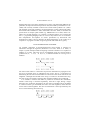
simple L-system example would be assigning consecutive numbers to a sequence of
modules in a string. This task can be accomplished using the context-sensitive
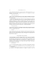
production B(m) < A(n) Æ B(m+1), as illustrated below for a string of N=4
modules:
We observe that it takes N–1 derivation steps for the information to propagate to the
end of an N-element string, as indicated by the arrows. This is a consequence of
determining the next state of each module as a function of the current state of its left
neighbour. Although each module in the string is rewritten in each derivation step,
the state of only one module is changed. The remaining modules are not affected.
L+C includes a construct that makes it possible to accelerate this information
transfer if the string is rewritten sequentially, from left to right, during a single
derivation step. Under this assumption, the next state of a module can be calculated
as a function of the (just calculated) next state of its left neighbour, rather than the
current state of that neighbour. The flow of information is then represented by the
arrows in the following derivation step:
THE L+C PLANT-MODELLING LANGUAGE
29
In order to refer to this new context in L-system productions, we use the symbol << .
A production that defines the above derivation can thus be written as
B(m) << A(n) Æ B(m+1).
In general, the predecessor of a production using new context in a derivation
proceeding from left to right has the following format:
new-left-context << strict-predecessor > right-context .
In an analogous manner, if a derivation step is performed from right to left, a
production predecessor with new context has the general format:
left-context < strict-predecessor >> new-right-context .
The left-context and right-context fields are optional. Motivated by the above
example, we refer to L-systems that use the new context construct as L-systems with
fast information transfer. Note that a production may only have one new context
field (i.e., either << or >>), depending on the derivation direction. Productions with
a new context field inconsistent with the current derivation direction are ignored.
FORMAT OF L+C PRODUCTIONS
The productions considered in the previous section were specified using a
mathematical L-system notation. In L+C, the arrow is replaced by the keyword
produce, which leads to production specification of the form
B(m) << A(n) : {produce B(m+1);}
In general, an L+C production has the syntax:
predecessor : {production body}
where the predecessor is specified as discussed in the previous section, and the
production body is a block of C++ code including one or more statements:
produce parametic-stringopt ;
Although the mathematically inspired arrow notation may appear more elegant than
the L+C notation, the latter is more flexible as a programming construct. For
example, an L+C production may include several alternative successors, as in the
construct:
B(m) << A(n) : {
m++;
if (m%3==0) produce C(m)B(m); else produce B(m);
}
In addition to assigning consecutive numbers to consecutive modules B(m), this
production inserts a module C(m) in front of every B(m) each time m is divisible
30
P. PRUSINKIEWICZ ET AL.
by 3. The traditional notation would require two separate productions to express the
same idea, which might be inefficient if the computations preceding production
application were much longer than the simple incrementation, m++.
L+C also supports a variant of the produce statement, denoted by keyword
nproduce. In contrast to produce, the execution of nproduce does not
terminate the application of a production. This makes it possible to construct the
successor of a production ‘piece by piece’. For example, using nproduce, the
previous production can be simplified to the form:
B(m) << A(n) : {
m++;
if (m%3==0) nproduce C(m);
produce B(m);
}
STRUCTURED PARAMETERS AND MODULE DECLARATIONS
In the above examples, we have only considered modules with a single numerical
parameter. L+C extends the previous definition of parametric L-systems
(Lindenmayer 1974; Prusinkiewicz and Hanan 1990; Prusinkiewicz and
Lindenmayer 1990; Hanan 1992) by allowing for the use of parameters of different
types, including user-definable data structures. To make this possible, L+C modules
are declared before use. Declaration specifies the number and types of parameters
that are associated with the given module type with the following syntax:
module identifier (parameter-listopt) ;
To illustrate the usefulness of structured parameters, let us consider the
following context-sensitive production in cpfg notation:
L(xl1,xl2,xl3,xl4,xl5) < A(x1,x2,x3,x4,x5) >
R(xr1,xr2,xr3,xr4,xr5) Æ A(x1,x2,x3,x4,x5+1)
This production operates on a module A with five real-valued parameters, and
increments the value of the last parameter by 1 if module A appears in the context of
modules L and R. Note that, due to the relatively high number of module parameters,
this production is difficult to read. The corresponding L+C code is:
struct data { float x1, x2, x3, x4, x5; };
module A(data); module L(data); module R(data);
L(dl) < A(d) > R(dr) :
{
d.x5 += 1.0;
produce A(d);
}
In this example, as in most simple programs, the L+C code is longer than the
equivalent cpfg code. Nevertheless, the use of structured module parameters offers
several advantages:
THE L+C PLANT-MODELLING LANGUAGE
31
x Long lists of parameter modules can be avoided. This results in a more legible
code.
x The L+C code is less error-prone. In cpfg it is easy to introduce an error by
inadvertedly skipping a parameter in a long parameter list.
x The L+C code is easier to modify. For example, if an additional parameter x6 is
needed to characterize modules L, R and A, in L+C it suffices to extend the
definition of the structure data. In contrast, in cpfg it is necessary to include x6
explicitly in the parameter list associated with each occurrence of these modules.
CONTROL OF L-SYSTEM PROGRAM EXECUTION
In principle, the notion of L-systems leads to a declarative programming style. Each
production is a statement of the form: “If a module and its neighbours match the
production predecessor then subsequent actions will be performed as specified in the
production body”. These actions thus depend on the state and context of the module
to which they apply, rather than a control flow mechanism as found in imperative
languages.
Nevertheless, L+C also includes elements of the imperative programming style.
The body of each production is specified as a sequence of statements based on C++.
Furthermore, there are four blocks of statements that are performed at specific points
of the derivation: at the beginning of the simulation (Start), at the beginning of
each derivation step (StartEach), at the end of each step (EndEach), and at the
end of the simulation (End). These blocks were already defined for cpfg (Hanan
1992), but play a more significant role in L+C because they may include statements
that affect the flow of the simulation.
One such pair of statements are calls to the predefined functions Forward()
and Backward(). These functions are typically used within the StartEach
block, and determine whether the derivation will proceed left-to-right or right-to-left
in the forthcoming step. As we have seen in the section "Fast information transfer",
the direction of the derivation is of critical importance in the case of fast information
transfer, because left new context can only be used when the derivation proceeds
left-to-right, and right new context can only be used when the derivation proceeds
right-to-left.
As the applicability of productions with new context depends on the direction of
the derivation, only a subset of the production set may apply in a given derivation
step. In the case of fast information transfer this subset may be established
implicitly, by ignoring productions with the new context that are incompatible with
the current direction of derivation. However, in many models it is convenient to
control the applicable production set explicitly (Frijters and Lindenmayer 1974;
Frijters 1976). To this end, L+C supports statements of the form
group group_id :
which divide the set of productions into subsets called groups (or tables in L-system
theory; cf. Rozenberg 1973; Ginsburg and Rozenberg 1975). A group statement
can be inserted before any production, and assigns a numerical label group_id to the
32
P. PRUSINKIEWICZ ET AL.
subset of productions that follow. This label remains in effect until the next group
statement or the end of the production list. The group statements are used in
conjunction with the function
UseGroup(group_id)
which is typically called within the StartEach block and defines the group of
productions to be used in the forthcoming step. By definition, productions in group 0
are used in all steps.
The notion of groups lends itself to the division of the simulation into a sequence
of phases, each characterized by the use of a specific production group. The
sequence of phases that constitute a simulation may be fixed, but it may also be
determined dynamically, with the next phase depending on the outcome of the
previous phase. For example, such a situation may occur if L-system productions are
applied iteratively, until some criterion of convergence is met. It may then be
desirable to interpret and visualize the result of a simulation graphically only after
convergence has been achieved. To this end, L+C supports the function
DisplayFrame()
which is typically called within the EndEach block to display the result of the latest
simulation step. Furthermore, as the number of iterations may be difficult to define a
priori, L+C supports the function
Stop()
which terminates the execution of the simulation at the end of the derivation step in
which it has been called. Examples of the constructs discussed in this and the
following sections will be given in the context of a complete L+C model (Section "A
Biomechanical example").
MULTIVIEW VISUALIZATION
In some applications, it is useful to display different aspects (views) of a simulation
concurrently (Roberts 2000). For example, one view may realistically represent a
developing plant, while another shows corresponding statistical information in the
form of a dynamically updated table or a histogram. In L+C, different views can be
displayed in separate windows, the contents of which are specified using subsets of
interpretation rules (Prusinkiewicz et al. 2000). Each subset is called a visual group,
and is identified by the statement
vgroup view :
A vgroup statement assigns the label view to the subset of interpretation rules that
follow it. A visual group is terminated by the next vgroup statement or the end of
the production list.
An important difference between the group and vgroup statements concerns
the execution of the affected productions. In addition to group 0, only one
THE L+C PLANT-MODELLING LANGUAGE
33
production group, specified by the latest call to the UseGroup() function, applies
to any particular simulation step. In contrast, interpretation rules in several visual
groups can be executed in each simulation step, provided that windows associated
with these groups are open. An L+C programmer may control which windows are
open using the function call
UseView(view).
Additional constructs are provided in L-studio and lpfg to determine the default size
and position of the windows, and to open and close them using menus.
INTERACTION WITH THE MODELS
Computational models are often used in simulated experiments in which model
attributes are modified to address ‘what if’-type questions. Models expressed in L+C
are conducive to such experiments, since the user can modify any aspect of the
model by changing the L-system code. In addition, L-studio and vlab provide
interactive tools that provide an interface for manipulating the numerical parameters
and functions incorporated in the model. These tools include user-configurable
virtual control panels and graphical function editors (Prusinkiewicz 2004).
The user may also explore models by directly manipulating their visual
representations on the screen. Such manipulations may mimic physical operations
such as pruning, girdling or pulling branches. The fundamental operation underlying
these manipulations is the selection of a module within the graphical representation
of the model. When the user selects a module with the mouse, a reserved module,
MouseIns() in L+C, is automatically inserted before the symbolic representation
of the selected module in the L-system string. The modeller specifies the response to
this event using a production that includes MouseIns()in the predecessor.
A BIOMECHANICAL EXAMPLE
To illustrate L+C constructs in the context of a complete program, let us consider
the biomechanical model of a growing pendulous branch proposed by Jirasek et al.
(2000) according to the ideas of Fournier (1989). Jirasek et al. observed that the
forces and torques involved in the bending, as well as the resulting reorientations
and displacements of internodes, can be considered signals that propagate between
plant modules and have local effects. This observation led to L-system
implementations of the biomechanical model, first in cpfg (Jirasek 2000) and later in
L+C (Taylor-Hell 2005). The L+C implementation makes use of almost all the
programming constructs specific to this language, and therefore provides a good
example of its features. In the model below, we ignore for simplicity the effects of
tropisms and secondary growth. We also assume that the model operates in 2D.
34
P. PRUSINKIEWICZ ET AL.
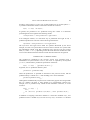
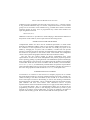
Figure 1. Geometry of branch bending. Left: representation of a branch with N=5
internodes, and the symbols used in the derivation of the formula for static equilibrium.
Right: the adjustment of internode orientation during the relaxation process
The point of departure in the model construction is the derivation of equations
that characterize branch shape in static equilibrium. We represent the branch as a
sequence of internodes (Figure 1a), beginning with a fixed internode and terminated
by an apex. The internodes are numbered from 1 (fixed proximal internode) to N
(distal internode), and connect nodes numbered 0 to N. Each internode is represented
as a vector ri si H i , where the number si denotes internode length, and the unit
vector H i denotes internode orientation. The position of node j with respect to node i
0 d i j d N is thus described by the vector
j
¦ rk .
R i, j
(1)
k i 1
We assume that the branch would be straight in the absence of gravity but bends
downward in the presence of gravity. To model this bending, we assume that each
node i is an elastic joint, subject to a torque IJ i . This torque is caused by gravity
acting on the overhanging part of the branch (positioned distally with respect to
node i). To simplify calculations, we assume that the mass of the branch is
concentrated in its nodes.
Let Fi mi g denote the force acting on node i with mass mi under gravitational
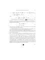
acceleration g . The torque IJ i is the sum of the torques exerted by the individual
masses positioned distally with respect to node i:
N
IJi
¦ R i, j u F j .
(2)
j i 1
The above equation expresses torques in global terms, in the sense that it
incorporates influences of masses mi that may be positioned far away from node i.
Nevertheless, torques acting on consecutive joints can be related to each other in
local terms. Specifically, the torque acting on node i 1 is equal to
THE L+C PLANT-MODELLING LANGUAGE
N
IJ i 1
¦R
N
i 1, j
u Fj
R i 1,i u Fi ri u ¦ F j j i
N
u Fj
i 1, j
ri u Fi j i 1
j i
N
¦R
35
¦ r R u F
i
j i 1
i, j
j
(3)
N
¦R
i, j
u Fj
ri u Ti IJ i ,
j i 1
where
N
Ti 1
¦F
N
Fi 1 ¦ F j
j
j i 1
Fi 1 Ti .
(4)
j i
In static equilibrium, a torque of magnitude W i
IJ i , acting on the node i, rotates
internode ri 1 by angle D i W i / N i with respect to internode ri . The parameter N i is
the rotational spring constant associated with node i. The geometry of the branch is
thus described by the equations:
Hi 1
Rotate( Hi ,Di ) ,
Pi 1
Pi si Hi ,
(5)
where the function Rotate( Hi ,Di ) changes the orientation of vector Hi by angle
Di (in 2D), and Pi is the position of mass mi.
To find the equilibrium, we use a relaxation method (Press et al. 1992, pp. 754755), which in this case consists of an iterative application of two steps:
Step 1. Given a sequence of internodes ri si H i , calculate torque W i acting on each
node. To this end, scan the branch in the proximal direction, and apply Equations 3
and 4 to consecutive nodes.
Step 2. Given the torques W i , adjust the orientation of each internode. To this end,
scan the branch in the distal direction. Given the adjusted orientation H i' of
internode i, first find the vector H i''1 that forms angle D i
W i / N i with respect to H i'
(Figure 1b). The vector E i 1 H i''1 H i 1 is the difference between the orientation
of internode i 1 calculated in the previous iteration step and the orientation that
would be required to achieve equilibrium. The adjusted orientation of internode i 1
is then defined as Hi' 1 Normalize(Hi' 1 kEi 1 ) . Parameter k controls the amount
of adjustment and thus affects the speed of convergence to the solution, and function
Normalize restores the result to the unit length. Furthermore, the magnitudes of
difference vectors are accumulated to form an error measure:
N
e
¦ Ei
i 0
.
(6)
36
P. PRUSINKIEWICZ ET AL.
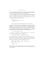
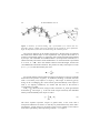
Figure 2. The sequence of phases in the simulation of a growing and bending branch. Similar
graphs are useful when defining the sequence of phases in other L+C models as well
The iteration ends when the error e falls below an assumed tolerance threshold.
Within this tolerance, the orientations of the internodes and positions of the nodes
then satisfy Equations 5. In the complete model of a growing branch, this is an
appropriate time to simulate a developmental step. The cycle of computation is
illustrated in Figure 2. The resulting L+C program is listed on the following pages.
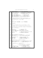
The program begins with the definitions of constants, variables and functions,
and declarations of data structures and modules (lines 1 to 53). The threedimensional vector V3f, which appears for the first time in the definition of the
gravity vector (line 10), is one of the types declared in the L+C header file
lpfgall.h. An example of a user-defined function follows (lines 12-22). Lines
55-97 present a typical example of the organization of computation. The statements
in the Start block (lines 57-67) initialize variables, set the initial phase of the
computation, and activate two different views of the model at the beginning of the
simulation. The statements in the StartEach block (lines 69-77) specify the
production group and derivation direction to be used in the forthcoming simulation
step. Finally, the statements in the EndEach block (lines 79-97) determine the
sequence of simulation phases according to Figure 2. As the number of iterations
needed to reach the equilibrium is not known in advance, the results are displayed
on demand using the DisplayFrame() function (line 89), once the error drops
below a threshold value maxerror (line 86). For similar reasons, the number of
simulation steps needed for the branch to grow to a desired length is not known in
advance. The simulation is thus terminated by a call to the Stop() function once
the branch has reached the maximum prescribed length (lines 136-139). The
derivation length statement (line 99) serves as a safeguard, specifying an
upper limit on the number of steps.
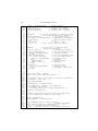
The Axiom statement (line 100) specifies the initial structure. First is the
Axes() module, which is used to draw coordinate axes in the Torques view.
Following it is the branch, which initially consists of a single internode followed by
an apex.
The L-system productions are divided into three groups. The PropagateLeft
and PropagateRight groups (lines 102-127), with a single production each,
iteratively compute the shape of the branch according to the mathematical analysis
presented earlier in this section. The conciseness of these productions illustrates the
expressive power of key constructs of L+C: context-sensitive productions, fast
information transfer, modules with structured parameters, and vector operations.
THE L+C PLANT-MODELLING LANGUAGE
1
2
3
4
5
6
7
8
9
10
11
12
13
14
15
16
17
18
19
20
21
22
23
24
25
26
27
28
29
30
31
32
33
34
35
36
37
38
39
40
41
42
43
44
45
46
47
48
49
50
51
52
53
54
55
56
57
58
59
60
61
62
#include <math.h>
#include <lpfgall.h>
const
const
const
const
const
const
const
//
//
//
//
//
C/C++ math header
declarations: L+C variables,
structures, functions, etc.
int MAX_N=30;
max number of internodes
float S=1.0;
internode length
float MASS=0.1;
// mass of a node
float KAPPA=4500.0;
// spring constant
float maxerror = 0.01; // error limit
float relax=0.5; // relaxation coefficient
V3f Gravity(0,-9.81,0); // gravity vector
/* Sample definition of functions on vectors:
Rotation of vector a in xy plane by angle alpha */
V3f VecRotate(V3f a, float alpha)
{
V3f c;
c.x = a.x * cos(alpha) - a.y * sin(alpha);
c.y = a.x * sin(alpha) + a.y * cos(alpha);
c.z = 0;
return c;
}
/* Analogous definitions of cross product, vector
length, and vector normalization should go here */
/* Declarations of structures, modules, and variables */
struct InternodeData
{
float s;
// internode length
float mass;
// node mass
float kappa; // rotational spring constant
float sigma_mass; // total mass to the right
float torque;
// torque from masses to the right
V3f P;
// proximal node position
V3f H;
// internode orientation
};
module Internode(InternodeData);
module Apex(int);
// int = number of internodes
module Axes(); // for visualizing coordinate axes
InternodeData iid;
int Phase;
float error;
int color;
//
//
//
//
initial internode data
computation phase
distance from equilibrium
current color index
/* Enumeration of computation phases */
#define PropagateLeft
#define PropagateRight
#define Grow
1 // accumulate masses, torques
2 // update angles, positions
3 // append internode
/* Organization of computation */
Start:
// At the beginning of simulation
{
// initialize non-zero variables:
iid.s = S;
// internode length,
iid.mass = MASS;
// node mass,
iid.kappa = KAPPA;
// rot. spring constant,
iid.H.x = 1;
// internode orientation,
37
38
63
64
65
66
67
68
69
70
71
72
73
74
75
76
77
78
79
90
81
82
83
84
85
86
87
88
89
90
91
92
93
94
95
96
97
98
99
100
101
102
103
104
105
106
107
108
109
110
111
112
113
114
115
116
117
118
119
120
121
122
123
124
P. PRUSINKIEWICZ ET AL.
Phase = PropagateLeft;
color = 1;
UseView(Branch);
UseView(Torques);
//
//
//
//
initial
initial
Display
Display
phase,
color index.
view "Branch"
view "Torques"
}
StartEach:
// At the beginning of simulation step
{
// set group and derivation direction:
UseGroup(Phase);
// set current group,
if (Phase == PropagateLeft) // depending on the phase
Backward();
// derive right-to-left
else
// or
Forward();
// left-to-right.
error = 0;
// Also, clear cumulative error.
}
EndEach:
// At the end of simulation step
{
// determine next phase:
switch (Phase) {
// consider prev. phase;
case PropagateLeft:
// after propagating left
Phase = PropagateRight;
// propagate right,
break;
case PropagateRight:
// after propagating right
if (error > maxerror)
// if error above limit
Phase = PropagateLeft; // propagate left
else {
// otherwise
DisplayFrame();
// display branch
Phase = Grow; }
// and grow,
break;
case Grow:
// after growing
Phase = PropagateLeft;
// propagate left;
++color;
// increment color index,
break;
}
}
derivation length: 1000000;
Axiom: Axes() Internode(iid) Apex(0);
/* Accumulate masses and torques using fast information
transfer to the left. */
group PropagateLeft:
Internode(id) >> Internode(idr) :
{
id.sigma_mass = id.mass + idr.sigma_mass;
id.torque = idr.torque +
VecCrossProd(idr.H, id.sigma_mass*Gravity).z ;
produce Internode(id) ;
}
/* Update node angles and internode positions using
fast information transfer to the right. */
group PropagateRight:
Internode(idl) << Internode(id) :
{
V3f NewEquilVector = VecRotate(idl.H,
id.torque/id.kappa);
V3f DifferenceVector = NewEquilVector - id.H;
error += VecLength(DifferenceVector);
id.H = VecNormalize(id.H + relax*DifferenceVector);
THE L+C PLANT-MODELLING LANGUAGE
125
126
127
128
129
130
131
132
133
134
135
136
137
138
139
140
141
142
143
144
145
146
147
148
149
150
151
152
153
154
155
156
157
158
159
160
161
162
163
164
165
166
167
168
169
170
171
39
id.P = idl.P + id.s*id.H;
produce Internode(id);
}
/* Append new internode unless maximum number reached.
Handle interaction with the model. */
group Grow:
Internode(id) < Apex(n):
{
id.P += id.s*id.H; // Calculate new internode position
if (n<=MAX_N)
// if internode limit not exceeded
produce Internode(id) Apex(n+1); // append
else
// otherwise
Stop();
// terminate simulation.
}
MouseIns() Internode(id): // If node selected by mouse
{
id.mass *= 3 ;
// increase its mass 3 times.
produce Internode(id);
}
/* Visualize simulation results */
interpretation:
group 0:
// display irrespective of phase
vgroup Branch :
// specification of view "Branch":
Internode(id) :
// draw an internode as a line
{
// and a circle
nproduce SetColor(color);
produce LineTo3f(id.P) Circle(id.mass);
}
vgroup Torques:
// specification of view "Torques":
Internode(id) :
// extend the plot of torques
{
id.P.y = -0.045*id.torque;
produce SetColor(color) LineTo3f(id.P);
}
Axes() :
// draw coordinate axes
{
nproduce SetColor(255) SB() F(20) EB();
produce SB() Right(90) F(25) EB();
}
The Grow group consists of two productions. The first production (lines 133140), describes the addition of a new internode to the branch and stops the
simulation once the maximum branch length has been reached. The second
production (lines 142-146) handles interaction with the model. If the user clicks on
an internode, the symbol MouseIns() is automatically inserted before the
corresponding Internode module in the L-system string. The production handles
this situation by incrementing the mass of the internode threefold and removing the
MouseIns() symbol from the string. This operation can be used to investigate the
impact of a fruit load on the branch shape, for example.
40
P. PRUSINKIEWICZ ET AL.
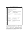
The remainder of the code (lines 148-171) is devoted to the visualization of
simulation results. Two windows are used for this purpose. The first window is
associated with the vgroup Branch and shows the shape of the growing branch.
The second window is associated with the vgroup Torques and shows the
distribution of torques along consecutive nodes of the branch. These views are
obtained using different interpretations of the same module Internode. The last
rule, with predecessor Axes() defined in the axiom, plays an auxiliary role of
displaying coordinate axes in the plot of torques. With a few additional lines of
code, we could also place numerical scales and labels on the axes.
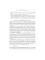
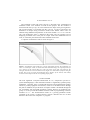
A snapshot of simulation results is shown in Figure 3.
Figure 3. Visualization of the model of a growing and bending branch. The simulation was
run in a ‘stroboscopic’ mode, in which consecutive simulation stages are superimposed. Left
view: changes of the branch shape over time. The mass of the node represented by the
enlarged circle has been increased interactively. Right view: distribution of torques along the
branch. Grey levels represent developmental stages (lengths) of the branch, and visually
associate branch shapes with the corresponding torque plots
CONCLUSIONS
The most significant conceptual advancement in L+C, compared to previous Lsystem-based languages, is fast information transfer. It significantly speeds up many
simulations, especially those of functional-structural and biomechanical models,
which rely on the propagation of hormones, resources or mechanical forces through
the plant. In addition, the specification of complex models is facilitated through the
use of modules with structured parameters, and the division of productions into
groups. L+C also provides the modeller with the wealth of programming constructs
available in C++. The biomechanical model of a growing pendulous branch
presented in the section "A Biomechanical example" illustrates the use of these
features in the context of a complete L+C program.
THE L+C PLANT-MODELLING LANGUAGE
41
L+C is well suited to the specification of models that incorporate a single aspect
of plant function within a developing plant structure. An open problem is the
construction of comprehensive models that incorporate several aspects, such as
genetics, partitioning of different resources, hormonal control, biomechanics and
development. The challenge is to devise a methodology, supported by appropriate
language constructs, that would make it possible to build such models in a wellstructured manner – with different model components specified, implemented and
tested independently, and easily combined into final synthetic models.
ACKNOWLEDGEMENTS
We thank Lynn Mercer, Jim Hanan and Alla Seleznyova for comments on the
manuscript. The support of this research by the Human Frontier Science Program
and the Natural Sciences and Engineering Research Council of Canada is gratefully
acknowledged.
REFERENCES
Allen, M.T., Prusinkiewicz, P. and DeJong, T.M., 2005. Using L-systems for modeling source-sink
interactions, architecture and physiology of growing trees: the L-PEACH model. New Phytologist,
166 (3), 869-880.
Fournier, M., 1989. Mécanique de l’arbre: maturation, poids propre, contraintes climatiques. Institut
National Polytechnique de Lorraine, Nancy. Ph.D. dissertation, Institut National Polytechnique de
Lorraine
Frijters, D., 1976. An automata-theoretical model of the vegetative and flowering development of
Hieracium murorum L. Biological Cybernetics, 24 (1), 1-13.
Frijters, D. and Lindenmayer, A., 1974. A model for the growth and flowering of Aster novae-angliae on
the basis of table <1, 0> L-systems. In: Rozenberg, G. and Salomaa, A. eds. L Systems. SpringerVerlag, Berlin, 24-52. Lecture Notes in Computer Science no. 15.
Ginsburg, S. and Rozenberg, G., 1975. TOL schemes and control sets. Information and Control, 27 (2),
109-125.
Hanan, J.S., 1992. Parametric L-systems and their application to the modeling and visualization of
plants. University of Regina, Regina. Ph.D. dissertation, University of Regina [http://
algorithmicbotany.org/papers/hanan.dis1992.pdf]
Jirasek, C.A., 2000. A biomechanical model of branch shape in plants expressed using L-systems.
University of Calgary, Calgary. M.Sc. thesis, University of Calgary
Jirasek, C.A., Prusinkiewicz, P. and Moulia, B., 2000. Integrating biomechanics into developmental plant
models expressed using L-systems. In: Spatz, H.C. and Speck, T. eds. Plant biomechanics 2000:
proceedings of the 3rd plant biomechanics conference, Freiburg-Badenweiler, August 27th to
September 2nd, 2000. Thieme, Stuttgart, 615-624. [http://algorithmicbotany.org/papers/
biomechanics00.pdf]
Karwowski, R., 2002. Improving the process of plant modeling: the L+C modeling language. University
of Calgary, Calgary. Ph.D. dissertation, University of Calgary [http://algorithmicbotany.org/
papers/radekk.dis2002.pdf]
Karwowski, R. and Lane, B., 2006. LPFG user’s manual. [http://algorithmicbotany.org/lstudio/
LPFGman.pdf]
Karwowski, R. and Prusinkiewicz, P., 2003. Design and implementation of the L+C modeling language.
Electronic Notes in Theoretical Computer Science, 86 (2), 1-19.
Lindenmayer, A., 1968a. Mathematical models for cellular interaction in development. Part 1: Filaments
with one-sided inputs. Journal of Theoretical Biology, 18 (3), 280-299.
Lindenmayer, A., 1968b. Mathematical models for cellular interactions in development. Part 2: Simple
and branching filaments with two-sided inputs. Journal of Theoretical Biology, 18 (3), 300-315.
42
P. PRUSINKIEWICZ ET AL.
Lindenmayer, A., 1971. Developmental systems without cellular interaction, their languages and
grammars. Journal of Theoretical Biology, 30, 455-484.
Lindenmayer, A., 1974. Adding continuous components to L-systems. In: Rozenberg, G. and Salomaa, A.
eds. L Systems. Springer-Verlag, Berlin, 53-68. Lecture Notes in Computer Science no. 15.
MČch, R., 2005. CPFG version 4.0 user's manual. Available: [http://algorithmicbotany.org/lstudio/
CPFGman.pdf] (30. May 2006).
Mündermann, L., Erasmus, Y., Lane, B., et al., 2005. Quantitative modeling of Arabidopsis development.
Plant Physiology, 139 (2), 960-968.
Perttunen, J., Sievänen, R., Nikinmaa, E., et al., 1996. LIGNUM: a tree model based on simple structural
units. Annals of Botany, 77 (1), 87-98.
Press, W.H., Teukolsky, S.A., Vetterling, W.T., et al., 1992. Numerical recipes in C: the art of scientific
computing. 2nd edn. Cambridge University Press, Cambridge. [http://www.nrbook.com/a/
bookcpdf.php]
Prusinkiewicz, P., 1999. A look at the visual modeling of plants using L-systems. Agronomie, 19 (3/4),
211-224.
Prusinkiewicz, P., 2004. Art and science for life: designing and growing virtual plants with L-systems.
Acta Horticulturae, 630, 15-28.
Prusinkiewicz, P. and Hanan, J., 1990. Visualization of botanical structures and processes using
parametric L-systems. In: Thalmann, D. ed. Scientific visualization and graphics simulation. Wiley,
Chichester, 183-201.
Prusinkiewicz, P., Hanan, J. and MČch, R., 2000. An L-system-based plant modelling language. In: Nagl,
M., Schürr, A. and Münch, M. eds. Applications of graph transformation with industrial relevance:
international workshop, AGTIVE'99 Kerkrade, The Netherlands, September 1-3, 1999. Springer,
Berlin, 395-410. Lecture Notes in Computer Science no. 1779.
Prusinkiewicz, P. and Lindenmayer, A., 1990. The algorithmic beauty of plants. Springer-Verlag, New
York.
Roberts, J.C., 2000. Multiple-view and multiform visualization. In: Erbacher, R., Pang, A., Wittenbrink,
C., et al. eds. Visual data exploration and analysis VII, San Jose CA, 24-26 January 2000. IS&T,
Bellingham, 176-185. Proceedings of SPIE no. 3960.
Rozenberg, G., 1973. TOL systems and languages. Information and Control, 23 (4), 357-381.
Taylor-Hell, J., 2005. Biomechanics in botanical trees. University of Calgary, Calgary. M.Sc. thesis,
University of Calgary [http://algorithmicbotany.org/papers/juliath.th2005.pdf]