Download Lecture

Lec 7 (2/20/02) Basic Molecular Dynamics (MD)
This lecture is an attempt to present a concise, self-contained discussion of the basic elements of
molecular dynamics (MD) simulation, as a read-me primer for the newcomer as well as a
summary of essentials for the initiated student who is not yet expert .
Outline of this lecture is as follows:
1.
2.
3.
4.
5.
6.
Defining the MD Method
The Pair Potential
Bookkeeping Matters
Properties Which Make MD Unique
Hands-On MD
Understanding Crystals and Liquids - An Example of an Application
1. Defining the MD Method
A working defintion of MD is: The process by which one generates the atomic trajectories of
a system of N particles by direct numerical integration of Newton's equations of motion
with appropriate specification of an interatomic potential and suitable initial and boundary
conditions.
To explain what we mean by this statement we consider our simulation model (system) to be N
particles enclosed in a region of volume V at temperature T. The positions of the N particles are
specified by a set of N vectors, {r (t)} = (r 1 (t), r 2 (t),..., r N (t)) , with r j (t) being the position of
particle j at time t. Knowing {r (t)} at various time instants means that we know how the
particles move at time evolves, or their trajectories. Our model system of particles has a certain
energy E which is the sum of kinetic and potential energies of the particles, E = K + U, where K
is the sum of individual kinetic energies
1 N 2
K = m∑ v j
2 j=1
and U is the prescribed interatomic potential mentioned above, U(r 1 , r2 ,...,r N ) . In general U
depends on the positions of all the particles in a complicated fashion. We will soon introduce a
simplifying approximation (assumption of pairwise interaction) which makes this most important
quantity much eaasier to handle.
To find the atomic trajectories in our model we need to solve the equations that the particle
positions vectors satisfy; this is just the Newton's equations of motion, F = ma, which everybody
knows from simple mechanics. While we are all familiar with the equations of motion of a
pendulum or a rolling body, the equations for motion for our N-particle is more complicated
because the equation for one particle is coupled to all the other equations through the potential
energy U. We see this readily when we write out the equations that we need to solve,
1
m
d2 rj
dt 2
= −∇ r j U({r }) , j = 1, ..., N
(1)
This dependence of the motion of one particle on the position of all the others is quite reasonable
since the force acting on one particle will change any time one of the other particles moves.
Eq.(1) looks deceptively simple, but it is as complicated as the famous N-body problem which we
do not know how to solve exactly when N is more than 2. On the other hand, we can solve (1)
numerically without too much difficulty. It is a system of second-order, non-linear ordinary
differential equations.
When we say in the above definition of MD that we want to integrate (1) to obtain the atomic
trajectories, we mean that we will divide the time interval of interest into many small segments,
each being a timestep of ∆ t . Given the initial condtion at time to, {r (t o )} , integration means we
can advance the system by increments of ∆ t ,
{r (t o )} → {r(to + ∆t)} → {r(to + 2∆t)} →...{r( to + Nt ∆t)}
(2)
where Nt is the number of timesteps making up the interval of integration.
How do we actually numerically integrate (1) for a given U? A simple way is to write a Taylor
series expansion,
r j (t o + ∆t) = r j (to ) + v j (t) ∆t +
1
2
a j (t)( ∆t) +...
2
(3)
Write a similar expansion for r j (t o − ∆t ) , then add the two expansions to obtain
r j (t o + ∆t) = −r j (t o − ∆t) + 2 r j (to ) + a j ( to )(∆t)2 +...
(4)
Notice that the left-hand side is what we want, namely, the position of particle j at the next
timestep ∆ t , whereas all the terms on the right-hand side are quantities evaluated at time to . The
positions at to and the timestep before we already know, so the question is what about the
acceleration of particle j at time to. For this we can make use of (1) and write F j ({r (t o )}) / m in
place of the acceleration, where F is just the right-hand side of (1). Eq.(4) is therefore the
integration of (1), that is, we march out in discrete time steps, one step at a time. We evaluate all
the terms on the right-hand side and thereby obtain the position at the next step, then repeat the
process to move another step, etc. There are more elaborate ways of doing this integrationbut the
basic idea of marching out in discrete steps is the same. The procedure just described is called
the Verlet central difference method. The procedure used in the MD code which we will
distribute in class makes use of a more accurate method called Gear Predicotr-Corrector. A more
accurate method allows one to take a larger value of ∆ t , which is certainly desirable, but this also
means one needs more menmory relative to the simpler method.
2
The time integrator is at the heart of MD simulation, since if one can advance the system of N
particles by one ∆ t , the process can be repeated as many times as one wants to generate a
sequence of positions (or trajectories) for as long an inerval as desired. These trajectories
(positions and velocities) are therefore the raw output of MD simulation. With such data one can
do all kinds of processing and obtain practically all the physical properties of interest. The flowchart for a typical MD simulation looks something like the following.
(a) → (b) → (c) → (d) → (e) → (f) → (g)
a = set particle positions b = assign particle velocities c = calculate force on each particle d = move particles by timestep ∆ t
e = save current positions and velocities f = if reach preset no. of timesteps, stop, otherwise go back to (c) g = analyze data and print results 2. The Pair Potential
To make the simulation tractable, it is common to assume the interatomic potential U can be
represented as the sum of pairwise interactions,
U(r 1 ,..., r N ) ≅
1
∑ V( rij )
2 i≠j
(5)
where rij is the separation distance between particles i and j. V is the pair potential of interaction;
it is a central force potential, being a function only of the separation distance between the two
particles. A very common pair potential used in atomistic simulations is one which describes the
van der Waals interaction in an insulator; it is of the form (known as the Lennard-Jones 6-12
potential)
 σ 12  σ  6 
V(r) = 4 ε   −
 r  
 r
3
(6)
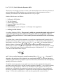
with parameters ε and σ . The most important features of this interaction are a short-range
repulsion which rises sharply (with inverse power of 12) at close interatomic separations, and an
attraction varying with the inverse power of 6. We can understand the repulsion as arising from
overlap of the electron clouds, and the attraction as being associated with the interaction between
the induced dipole in each atom (the so-called London dispersion interaction). The value of 12
for the first exponent has no special significance, as the repulsive term could just as well be
represented by an exponential, whereas the second exponent results from quantum mechanical
calculations and therefore should not be modified. The importance of short-range repulsion is
that this is necessary to give the system a certain size or volume (density), without which the
particles can collapse onto each other, whereas the attraction is necessary for cohesion of the
system of particles, without which the particles will all fly away from each other. Both are
necessary for solids and liquids to have the physical properties that we know from everyday
experience.
3. Bookkeeping Matters
Our simulation system is typically a cubical cell in which particles are placed either in a very
regular manner, as in modeling a crystal lattice, or in some random manner, as in modeling a gas
or liquid. The number of particles in the simulation cell is quite small. For the homework
assignment the value ranges from 32 to 864 in the order of 32, 108, 256, 500, 864. These come
about because the class code (which we call hailecode) is designed for a face-centered cubic
lattice in which there are 4 atoms per primitive cell. Thus, if our cube has s cells along each side,
then the number of particles in the cube will be 4s3. The above numbers then correspond to
cubes with 2, 3, 4, 5, and 6 cells along each side respectively.
Once we choose the number of particles we want to simulate, the next step is to choose what
system density we want to study. Choosing the density is equivalent to choosing the system
volume since density n = N/V, where N is the number of particles and V is the volume.
Hailecodeuses dimensionless reduced units, so reduced density DR has typical values around 1.0
- 1.2 for solids, and 0.6 - 0.85 for liquids. For reduced temperature TR we recommend values of
0.4 - 0.7 for solids, and 0.9 - 1.3 for liquids. Notice that assigning particle velocities in (b) above
is tantamount to setting the system temperature.
For simulation of bulk systems (no free surfaces) it is conventional to use the periodic boundary
condition (pbc). This means the cubical cell is surrounded by 26 identical image cells. For
every particle in the simulation cell, there correspond an image particle in each image cell. The
26 image particles move in exactly the same manner as the actual particle, so that if the actual
particle should happen to move out of the simulation, the image particle in the image cell
opposite to the exit side will move in (and becomes the actual particle, or the particle in the
simulation cell) just as the original particle moves out. The net effect is that with pbc particles
cannot be lost or gained. In other words, the particle number is conserved, and if the simulation
cell volume is not allowed to change, the system density remains constant.
Since in the pair potential approximation, the particles interact two at a time, a procedure is
needed to decide which pair to consider among the pairs between actual particles and between
actual and image particles. The minimum image convention is a procedure where one takes the
nearest neighbor to an actual particle, irregardless of whether this neighb or is an actual particle
4
or an image particle. Another approximation which is useful to keep the computations to a
manageable level is to introduce a force cutoff distance beyond which particle pairs simply do
not see each other. In order not to have a particle interact with its own image, it is necessaary to
ensure that the cutoff distance is less than half of the simulation cell dimension.
Another bookkeeping device often used in MD simulation is a Neighbor List which keeps track
of who are the nearest, second nearest, ... neighbors of each particle. This is to save time from
checking every particle in the system every time a force calculation is made. The List can be
used for several time steps before updating. Each update is expensive since it involves NxN
operations for an N-particle system. In low-temperature solids where the particles do not move
very much, it is possible to do an entire simulation without or with only a few updating, whereas
in simulation of liquids, updating every 5 or 10 steps are quite common. For further discussions
of bookkeeping matters, the student should see the MD Primer of J. M. Haile (1980).
4. Properties Which Make MD Unique
There is a great deal that can be said about why MD is such a useful simulation technique.
Perhaps the most important statement is that in this method (consider classical MD for the
moment, as opposed quantum MD) one follows the atomic motions according to the principles of
classical mechanics as formulated by Newton and Hamilton. Because of this, the results are
physically as meaningful as the potential U that is used. One does not have to apologize for any
approximation in treating the N-body problem. This means that whatever mechanical,
thermodynamic, and statistical mechanical properties that the system of N particles should have,
they are still present in the data. Of course how one extracts these properties from the output of
the simulation – the atomic trajectories – will determine how useful is the simulation. Before any
conclusions can be made, one needs to get in the question of how various properties are to be
obtained from the simulation data. Thus if we think of MD simulation as an ‘atomic video’ of the
particle motion (one which we can see as a movie), there is a great deal of realistic details in the
motions themselves, but how to extract the information in a scientifically useful is up to the
viewer. And an experienced viewer can get much more useful information than an inexperienced
one!
The above comments aside, we list here a number of basic reasons why MD simulation is so
useful (or unique). These are meant to guide the thinking of the student and encourage the
student to discover and appreciate the many interesting and significant aspects of this technique
on your own.
(a) Unified study of all physical properties. Using MD one can obtain thermodynamic,
structural, mechanical, dynamic and transport properties of a system of particles which can be
a solid, liquid, or gas. One can even study chemical properties and reactions which are more
difficult and will require using quantum Md.
(b) Several hundred particles are sufficient to simulate bulk matter. While this is not always true,
it is rather surprising that one can get quite accurate thermodynamic properties such as
equation of state in this way. This is an example that the law of large numbers takes over
quickly when one can average over several hundred degrees of freedom.
5
(c) Direct link between potential model and physical properties. This is really useful from the
standpoint of fundamental understanding of physical matter. It is also very relevant to the
structure-property correlation paradigm in materials science.
(d) Complete control over input, initial and boundary conditions. This is what gives physical
insight into complex system behavior. This is also what makes simulation so useful when
combined with experiment and theory.
(e) Detailed atomic trajectories. This is what one can get from MD, or other atomistic simulation
techniques, that experiment often cannot provide. This point alone makes it compelling for
the experimentalist to have access to simulation.
We should not leave this discussion without reminding ourselves that there are significant
limitations to MD. The two most important ones are:
(a) Need for sufficiently realistic interatomic potential functions U. This is a matter of what we
really know fundamentally about the chemical binding of the system we want to study.
Progress is being made in quantum and solid-state chemistry, and condensed-matter physics;
these advances will make MD more and more useful in understanding and predicting the
properties and behavior of physical systems.
(b) Computational capabilities constraints. No computers will ever be big enough and fast
enough. On the other hand, things will keep on improving as far as we can tell. Current limits on
how big and how long are a billion atoms and about a microsecond in brute force simulation.
5 Hands-On MD
‘Talk is cheap’ when it comes to modeling and simulation. What is not so easy is to ‘just do it’.
In this spirit we want everyone to get your hands on an MD simulation code and just play with it.
We are distributing to the class a hardcopy of a very useful writeup – A Primer on the
Computer Simulation of Atomic Fluids by Molecular Dynamics, J. M. Haile (1980). Treat
this like a User’s Manual for the code that you can download from an Athena Course Locker, in
this case the course is 22.53 (Statistical Processes and Atomistic Simulation), a graduate subject
taught in Course 22.
Here are the instructions for getting the code, for which we suggest the name hailecode, into your
own directory.
1. In your own Athena directory, type
add 22.53
cd /mit/22.53/fall00/md_tutorial/tutor
add matlab
matlab –nojvm &
6
When presented with a Menu, choose #1 tutorial if this is your first time. Choose #3 when you are ready to download the Code (which will be named hailecode) Go back to your own directory and type cd ~/22.53 g77 –O3 moldyn_sim.f –o hailecode Now hailecode should be loaded into your directory.
To run the Code, type
./hailecode
then follow the prompt to specify 5 input parameters When simulation is done, you can plot the results by returning to the Matlab terminal and type cd ~/22.53
plotdata
You will get three figures plotted out on the screen.
2. To make future runs from your Athena directory, type
cd ~/22.53 g77 –O3 moldyn_sim.f –o hailecode ./hailecode Follow prompt, when run is finished, you can go to plot by typing
Add matlab
Matlab –nojvm &
Wait for Matlab window, type at the prompt >>
Cd ~/22.53
Plotdata
Get three figures on screen as before.
5. Understanding Crystals and Liquids – An Example of an Application
There are many ways one can study the structure and dynamics of solids and liquids at the
atomistic level using MD. In fact, this is one of main reasons why MD has become so well
respected for what it can tell about how atoms and molecules are distributed in condensed and
how they move about in response to thermal excitations or external conditions such as pressure.
7
There will be many examples of this kind that will be discussed in this subject. For now we will focus on two fundamental properties of condensed matter, one pertaining to the structure and the other pertaining to motion. Imagine we do a simulation with hailecode where we specify the following input: NP = number of particles NEQ = number of timesteps for equilibration MAXKB = number of timesteps for the actual simulation run TR = reduced temperature DR = reduced density The output of hailecode for this set of input parameters can be plotted in Matlab by following the above instructions. What you will get are three plots. Fig. 1 is a composite of three graphs showing the variation of pressure, potential energy, and temperature with time as the simulation evolves. This information is useful to make sure that the system is well equilibrated and that nothing strange is happening during the entire simulation. These graphs are like the meters on the wall of a reactor control room, showing how the pressure and temperature of the reactor are varying instantaneously during operation. Although important, they do not tell us anything about what is going on with the atoms inside the reactor. Figs. 2 and 3 are the plots that we want to study in detail. They are respectively a plot of the 2
<square displacement> function which we will denote as < ∆r > , and the radial distribution function g(R). Through these two functions we can understand quite a bit about solids and liquids. 2
(a) The Square Displacement function < ∆r >
This quantity is defined on p. 28 in the Haile Primer and further discussed on p. 36.
< ∆r 2 >=
1
2
[r i (t) − r i (0)]
∑
N i
This is eq. (3.34) in the Primer. Here r i (t) is the position of particle i at time t, so the square of
the vector difference is the distance that particle i has moved during the time interval t, and if we
average over all the particles this then gives the mean square distance that the particles have
moved during time t. So Fig. 2 is a plot of < ∆r 2 > as a function of t.
2
For any physical system < ∆r > should start at zero at t = 0 and in a few timesteps increase up
to some finite value. If the system is a solid, then the value of < ∆r 2 > after some time, say a
couple of hundred timesteps, no longer increases with time since in a solid, like a crystal, all the
atoms are bound to some local position and each atom undergoes small amplitude vibrational
motion centered around its local position. So we expect < ∆r 2 > to just fluctuate in time but not
showing any significant increase as the simulation proceeds. In contrast, if the system is a liquid,
then we expect all the atoms to be able to diffuse away from whatever position it had previously
as in Brownian motion. This then means that < ∆r 2 > should increase with time linearly when
its movements have settled into the classic form of diffusion. This simple and intuitive
8
2
discussion of the two kinds of basic behavior of < ∆r > now allows us to interpret the
simulation output whenever we make a simulation run.
(b) The Radial Distribution Function
This quantity is defined on p. 54 of the Primer. One starts by noting
g(r) = ρ (r) / ρ
where ρ (r) is the local number density. For the hailecode, DR is just the dimensionless density
ρσ 3 . By the way, the dimensionless temperature TR is just k BT / ε , where k B is the Boltzmann's
constant. Recall that σ , ε are the two parameters of the Lennard-Jones potential model. Now
hailecode calculates g(r) according to the expression
g(r) =
< N(r ± ∆r / 2) >
V(r ± ∆r / 2)ρ
where the numerator is the average number of particles in a spherical shell of radius r and
thickness ∆r , with the shell centered on one of the particles (any particle is as good as any other)
in the system, and V in the denominator is the volume of this shell.
What show g(r) look like if one plots it as a function of r? This is shown on p. 39 in the Primer.
The function g(r) shows several peaks, which can be very sharp or quite broad depending on the
state of the system, that is, a low-temperature crystal (very sharp peaks) or a high-temperature
liquid (very broad peaks). Thus, g(r) is the function that reveals the atomic structure of the
system being simulated.
In the case of the output from hailecode we can even predict where the peaks should be located in
the case of a low-temperature crystal. This is because the atoms are put into the simulation cell in
the positions of a face-centered cubic lattice. It is known that in the primitive unit cell of fcc, one
has 4 atoms in the cell. Sitting on any of the particles one can look around the surroundings in
the lattice and count up the number of nearest neighbor, second nearest neighbor, third neighbor,
..., as well as the distances between the central particle and its various neighbors. The number of
neighbors should be 12, 6, 24, and 12 for the first four neighbors, and their corresponding
separations should be the positions of where the peaks show up in g(r). Checking this out
explicitly is left as an excercise for the interested student.
We have given some hints here as to how one can learn something about the structure and
dynamics of systems of particles by doing MD simulation. We would like the student to explore
further your own, perhaps guided by the homework assignment. You should play around with
using different values for the input parameters. A lot more can be said, for now you might
consider the following suggestions.
NP = 32, 108, 256, 500, 864. Any one of the these values will work. Obviously a small system
will run faster which means you get the results back right away if you use a 32-particle
simulation cell as opposed an 864-particle cell. The latter generally takes less than 5 minutes
according to my experience.
9
NEQ = 1000. Use this default value. We can talk about doing something different later.
MAXKB = 2000 for a short run, 10000 for a longish run.
TR = 0.4 - 0.7 for crystal, 0.9 - 1.2 for liquid
DR = 0.9 - 1.2 for crystal, 0.6 - 0.9 for liquid
You should keep in mind that the larger the number of particles and the longer run time will give
you smoother and higher-quality results. The cost is that you have to wait a bit. Also, if you pick
combinations of TR and DR values which are between normal solids and liquids, then the system
can try to melt or freeze, and then you will results which can deviate from the typical behavior
discussed. There is much that you will learn by exploring on your own. Have fun and let us
know how you are doing!
10